1

ERRORS AND ERROR PROPAGATION INTRODUCTION: Laboratory experiments involve taking measurements and using those measurements in an equation to calculate an experimental result. It is also necessary to know how to estimate the uncertainty, or error, in physical measurements and to know how to use those uncertainties to calculate the error in the experimental result. TYPES OF EXPERIMENTAL ERRORS Experimental errors can generally be classified into three types: personal, systematic, and random. Personal Errors These errors arise from personal bias of carelessness in reading an instrument, in recording data, or in calculations, and parallax in reading a meter. Of these, only parallax errors can be estimated and used in error propagation. Effort should be made to eliminate experimental errors. (When looking at non-digital meter, there is a small distance between the needle and the scale. As a result, the reading will change as the observer’s eye position changes from side to side. This apparent change in reading, due to the change in position of the observer’s eye, is called parallax.) Systematic Errors Errors of this type result in measured values which are consistently to high or to low. Conditions which lead to systematic errors are as follows: 1. An improperly calibrated instrument such as a thermometer which consistently reads 99ºC in boiling water instead of 100ºC. 2. A meter, micrometer, vernier caliper, or other instrument which was not properly zeroed or for which the zero correction factor was not considered. 3. Theoretical errors due to a simplified mathematical model for the system which consistently gives a calculated value different from the calculated value predicted from a more accurate mathematical model. Random Errors Random errors result from unknown and unpredictable variations in experimental measurements. Possible sources of random errors are:

2

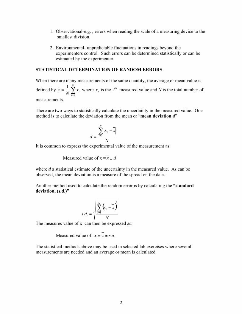
1. Observational-e.g. , errors when reading the scale of a measuring device to the smallest division. 2. Environmental- unpredictable fluctuations in readings beyond the experimenters control. Such errors can be determined statistically or can be estimated by the experimenter. STATISTICAL DETERMINATION OF RANDOM ERRORS When there are many measurements of the same quantity, the average or mean value is

defined by !=

=N

i

ix

Nx

1

_ 1 where ix is the ith measured value and N is the total number of

measurements. There are two ways to statistically calculate the uncertainty in the measured value. One method is to calculate the deviation from the mean or “mean deviation d”

N

xx

d

N

i

i!=

"

= 1

It is common to express the experimental value of the measurement as: Measured value of x = dx ± where d a statistical estimate of the uncertainty in the measured value. As can be observed, the mean deviation is a measure of the spread on the data. Another method used to calculate the random error is by calculating the “standard deviation, (s.d.)”

( )

N

xx

ds

N

i

i

2

1..

!=

"

=

The measures value of x can then be expressed as: Measured value of ..dsxx ±= The statistical methods above may be used in selected lab exercises where several measurements are needed and an average or mean is calculated.

3

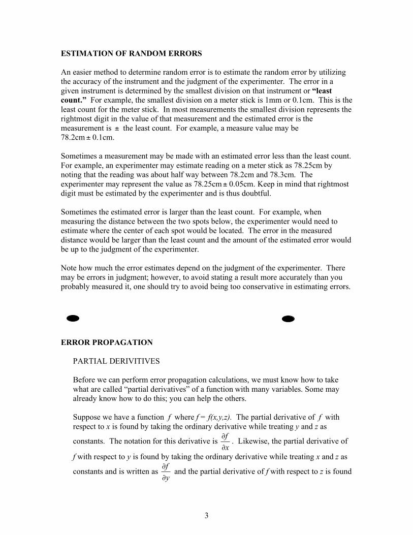
ESTIMATION OF RANDOM ERRORS An easier method to determine random error is to estimate the random error by utilizing the accuracy of the instrument and the judgment of the experimenter. The error in a given instrument is determined by the smallest division on that instrument or “least count.” For example, the smallest division on a meter stick is 1mm or 0.1cm. This is the least count for the meter stick. In most measurements the smallest division represents the rightmost digit in the value of that measurement and the estimated error is the measurement is ± the least count. For example, a measure value may be 78.2cm± 0.1cm. Sometimes a measurement may be made with an estimated error less than the least count. For example, an experimenter may estimate reading on a meter stick as 78.25cm by noting that the reading was about half way between 78.2cm and 78.3cm. The experimenter may represent the value as 78.25cm± 0.05cm. Keep in mind that rightmost digit must be estimated by the experimenter and is thus doubtful. Sometimes the estimated error is larger than the least count. For example, when measuring the distance between the two spots below, the experimenter would need to estimate where the center of each spot would be located. The error in the measured distance would be larger than the least count and the amount of the estimated error would be up to the judgment of the experimenter. Note how much the error estimates depend on the judgment of the experimenter. There may be errors in judgment; however, to avoid stating a result more accurately than you probably measured it, one should try to avoid being too conservative in estimating errors.

ERROR PROPAGATION

PARTIAL DERIVITIVES Before we can perform error propagation calculations, we must know how to take what are called “partial derivatives” of a function with many variables. Some may already know how to do this; you can help the others. Suppose we have a function f where f = f(x,y,z). The partial derivative of f with respect to x is found by taking the ordinary derivative while treating y and z as

constants. The notation for this derivative is x

f

!

! . Likewise, the partial derivative of

f with respect to y is found by taking the ordinary derivative while treating x and z as

constants and is written as y

f

!

! and the partial derivative of f with respect to z is found

4

by taking the ordinary derivative while treating x and y as constants and is written as

z

f

!

! .

As an example, let 325 yzxf = . Then ( )32

5 yzxxx

f

!

!=

!

! = 3

2

3105 xyz

x

xyz =

!

!

Convince yourself that 325 zx

y

f=

!

! and that 2215 yzx

z

f=

!

! .

ABSOLUTE AND RELATIVE ERRORS Absolute Error: When an error is estimated in a measured value of x it will be designated as x!± (delta x). x! has the same units as x and is called the absolute error in x. For example, if

cmcmx 1.00.2 ±= , the absolute error is cmx 1.0=! .

Relative Error: The ratio of the absolute error x! to the measured value x, x

x! , is

called the relative error. It is usually represented as a percent. For example, the

relative error in the above example is %505.00.2

1.0

0.2

1.0===

cm

cm

(note, there are times when it is necessary to go from relative error back to absolute error: xerrorx

relative=! )

COMPUTATION OF ERROR & PERCENT ERROR For a function ( )zyxff ,,= , the absolute error in f, f! , is defined as:

!"

!#$

!%

!&'

()

*+,

-./

012

3

4

4+(

)

*+,

-../

0112

3

4

4+(

)

*+,

-./

012

3

4

4=

222

zz

fy

y

fx

x

ff 5555

The relative error in f would thus be

!"

!#$

!%

!&'

()

*+,

-./

012

3

4

4+(

)

*+,

-../

0112

3

4

4+(

)

*+,

-./

012

3

4

4=

222

1z

z

fy

y

fx

x

f

ff

f555

5

5

The percent error in f = 100f

f

!"

EXAMPLE 1: Using the function we used as an example for partial derivatives, we would have

( ) ( ) ( ){ }2222322315510 zyzxyzxfxyzf !!!! ++=

thus !"

!#$

!%

!&'

(()

*++,

-+((

)

*++,

-+((

)

*++,

-=

2

32

222

32

322

32

3

5

15

5

5

5

10z

yzx

yzxy

yzx

zxx

yzx

xyz

f

f...

. which when

simplified becomes

!"

!#$

!%

!&'

()

*+,

-+((

)

*++,

-+(

)

*+,

-=

222

32

z

z

y

y

x

x

f

f ....

[Or, you may choose to calculate and f f! separately and then divide them in numerical form.] Note that the quantities in the parentheses are just the percent errors multiplied by the exponent for that particular variable. Suppose we have the experimental values for x, y, and z as:

cmcmx 1.00.3 ±= , cmcmy 1.02.5 ±= , and cmcmz 1.04.2 ±= . We would thus have the percent error in f as:

( )( ) ( )( )

!"

!#$

!%

!&'

()

*+,

-+(

)

*+,

-+(

)

*+,

-=

222

4.2

1.03

2.5

1.0

0.3

1.02

f

f. = 0.143 ≈15%

Note that the % error is rounded up to the nearest whole number. Since it is just an estimate, we can not justify more accuracy in the error. EXAMPLE 2:

Suppose c

baV

2253 +

= where ( )cma 1.02.8 ±= , ( )cmb 1.05.6 ±= , and

( )cmc 1.01.5 ±=

6

Thus !"

!#$

!%

!&'

()

*+,

-./

012

3

4

4+(

)

*+,

-./

012

3

4

4+(

)

*+,

-./

012

3

4

4=

222

cc

Vb

b

Va

a

VV 5555

where c

a

a

V 6=

!

! ,c

b

b

V 10=

!

! , and 2

2253

c

ba

c

V +!=

"

" ; or,

!"

!#$

!%

!&'

()

*+,

-../

0112

3 ++(

)

*+,

-./

012

3+(

)

*+,

-./

012

3=

2

2

2222

53106c

c

bab

c

ba

c

aV 4444

Notice that the negative sign in c

V

!

! does not matter since it is squared.

Now

!!

"

!!

#

$

!!

%

!!

&

'

((((

)

*

++++

,

-

.

.

.

.

/

0

1111

2

3

+

+

+

((((

)

*

++++

,

-

.

.

.

.

/

0

1111

2

3

++

((((

)

*

++++

,

-

.

.

.

.

/

0

1111

2

3

+=

2

22

2

222

22

2

2253

53

53

10

53

6

c

c

ba

c

ba

b

c

ba

c

b

a

c

ba

c

a

V

V444

4

Or,

( )( )( )( ) ( )( )

( )( )( )( ) ( )( ) !"

!#$

!%

!&'

()

*+,

-+

(()

*

++,

-../

0112

3

++

(()

*

++,

-../

0112

3

+=

22

22

2

221.5

1.01.0

5.652.83

5.6101.0

5.652.83

2.86

V

V4 =5.5%

≈6% (<= the percent error) The final results would be given as %681 ±= cmV

!"

!#$

!%

!&'

()

*+,

-+(

)

*+,

-./

012

3

++(

)

*+,

-./

012

3

+=

22

22

2

2253

10

53

6

c

cb

ba

ba

ba

a

V

V 444

4

7

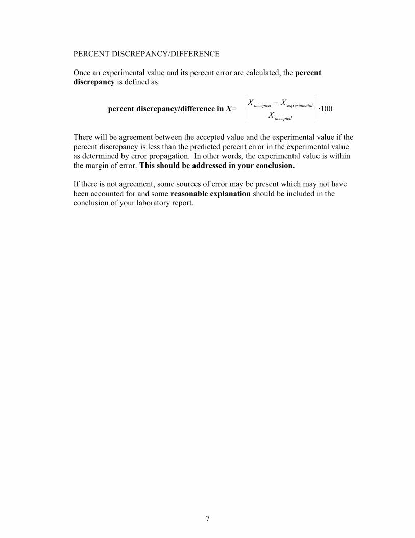
PERCENT DISCREPANCY/DIFFERENCE Once an experimental value and its percent error are calculated, the percent discrepancy is defined as:

percent discrepancy/difference in X= accepted

erimentalaccepted

X

XXexp

!100!

There will be agreement between the accepted value and the experimental value if the percent discrepancy is less than the predicted percent error in the experimental value as determined by error propagation. In other words, the experimental value is within the margin of error. This should be addressed in your conclusion. If there is not agreement, some sources of error may be present which may not have been accounted for and some reasonable explanation should be included in the conclusion of your laboratory report.

8

ERROR PROPAGATION EXERCISES Determine the calculated value using the given values in the given equations. Be sure to include the units in your answer. Using the error propagation method described above, calculate the percent error in the calculated value. For this exercise, your percent error is to be given to two significant figures. Hand in this answer sheet. Work the problems neatly on scratch paper and staple your work to this sheet. 1. A=xy, cmcmx 1.00.3 ±= , cmcmy 1.00.4 ±= ______________± ________ 2. f=x+y, for x and y given in problem # 1 ______________± ________ 3. f=x-y, for x and y given in problem # 1 ______________± ________ 4. z=3x+2y, for x and y given in problem # 1 ______________± ________

5. 2

2

t

hg = for %300.2 ±= mh , %4630.0 ±= st ______________± ________

6. k

MT !2= , %65.2 ±= KgM , %2

100±=

m

Nk ______________± ________

7. ( )32

00.5ML

gcmd !!

"

#$$%

&= , %20.30 ±= gM , ( )cmL 2.03.20 ±= ___________± ________

8. 22

yxz += , %20.3 ±= cmx , %20.4 ±= cmy ______________± ________

9. ( )C

bcmaz

2325 !

= , %10.2 ±= cma , %10.3 ±= cmb , %20.11 ±= cmC

______________± ________ 10. !sindh = , mmd 05.000.1 ±= , oo

110 ±=! ______________± ________