ERRORS IN SURVEY REPORTS OFCONSUMPTION EXPENDITURES

Erich Battistin

THE INSTITUTE FOR FISCAL STUDIESWP03/07

Errors in Survey Reports of Consumption

Expenditures

Erich Battistin∗

Institute for Fiscal Studies, London

6th May 2003

Abstract

This paper considers data quality issues for the analysis of consumptioninequality exploiting two complementary datasets from the Consumer Ex-penditure Survey for the United States. The Interview sample follows surveyhouseholds over four calendar quarters and consists of retrospectively askedinformation about monthly expenditures on durable and non-durable goods.The Diary sample interviews household for two consecutive weeks and in-cludes detailed information about frequently purchased items (food, personalcares and household supplies). Each survey has its own questionnaire andsample. Information from one sample is exploited as an instrument for theother sample to derive a correction for the measurement error affecting ob-served measures of consumption inequality. Implications of our findings areused as a test for the permanent income hypothesis.

Keywords: Consumption Inequality; Measurement Error; Permanent Income Hy-pothesis

JEL Classification: C13, C42, D12, D91

∗First draft 11th February 2002. This paper benefited from useful discussions with GordonAnderson, Orazio Attanasio, James Banks, Richard Blundell, Martin Browning, Hide Ichimura,Arthur Kennickell, Costas Meghir, Bruce Meyer, Enrico Rettore, Guglielmo Weber and fromcomments by audiences at Padova University, Cemmap (London), ESPE 2002, 10th InternationalConference on Panel Data and NBER Summer Institute 2002. Address for correspondence: Insti-tute for Fiscal Studies, 7 Ridgmount Street, London WC1E 7AE - UK. E-mail: erich b@ifs.org.uk.

1

EXECUTIVE SUMMARY

This paper aims to quantify the effect of reporting errors affecting diary-basedand recall-based data on non-durable expenditure. It is likely that not all thecommodities entering non-durable expenditure are well reported exploiting onlyone of these two survey methodologies. Expenditures on frequently purchased,smaller items are presumably more accurate using diaries while recall data are moreappropriate for large expenditures or expenditures occurring on a regular basis.

It turns out that neither diary nor recall-based data alone provide a reliableaggregate measure of total expenditure on non-durables. Ideally, the estimation oftotals at micro-level would require information on different consumption categoriesobtained with the most appropriate methodology. The Family Expenditure Surveyfor the United Kingdom represents a notable implementation of this strategy.

One might argue that for any practical purpose these alternative data collec-tion strategies lead to consistent results in the estimation of economic models ofconsumption behavior. Unfortunately, evidence from the literature suggests thatconclusions are strongly related to the information being used. This problem is ad-dressed by looking at micro data from two independent samples of households fromthe Consumer Expenditure Survey for the Unites States. This survey represent aunique source of data because it consists of diary an recall information collected onthe same set of items, although it refers to separate samples of households.

The comparison of the two surveys based on the overlap in coverage of expen-ditures offers insights for the effects of collection modes on data quality. Picturesemerging from the two surveys are very different, both with respect to mean expen-diture and, more importantly, with respect to indices of inequality. More precisely,while the differences in mean expenditure are roughly constant over time, consump-tion inequality presents different levels and trends in the two surveys. This evidenceis reconciled using integrated diary and recall information to characterize the mostlikely pattern of consumption for cohorts of individuals defined by their age.

This procedure allows us (i) to define an improved measure for mean and vari-ance of non-durable expenditure over the 1990s and (ii) to characterize the mea-surement error affecting the commodities whose quality is doubtful according toother studies in the literature. The implications of our findings for the estimationof inequality indices are discussed, with an application to permanent income mod-els. In particular, we show that using diary and recall data to improve the qualityof household consumption the permanent income hypothesis cannot be rejected.

2

1 INTRODUCTION

Data quality is an issue of longstanding concern among researchers interested intesting the implications of theoretical models of consumption over the life cycle.

The empirical analysis of these models requires reliable micro-data on expen-ditures at household or individual level. In many countries expenditure data areregularly collected either by diaries covering purchases made within a short periodof time (typically one or two weeks) or by means of retrospectively asked questionson the usual spending over a longer period.

There is a consensus that the time-consuming task required by diaries producesgood quality expenditure data for small items, while recall questions should beasked for bulky items (major consumer durables: real property, automobiles andmajor appliances) or for those components either having regular periodic billing orinvolving major outlays (such as transportation or rent).

For this reason diary surveys are designed to obtain detailed recordings of ex-penditures on small, frequently purchased items which are normally difficult torecall. Such an idea is not only intuitively clear, but it is also supported with evi-dence from cognitive studies and from the comparison of aggregated consumptionmeasures with national account data.

On the other hand, the drawback of such an evidence is that neither diary norrecall based data alone provide a reliable aggregate measure of total consumption.One might argue that for any practical purpose these two alternative designs leadto consistent results, but unfortunately this is not the case. For example, thereis some evidence that recall consumption data lead to potentially misleading re-sults in analyzing household saving behavior (Battistin et al. 2003). Other studiesdemonstrate how available consumption data can be unsuitable for the analysis ofthe permanent income (life cycle) hypotheses and how adjustments provide greaterconsistency concerning the time series properties of consumption (Wilcox 1992 andSlesnick 1998). Browning et al. (2002) provide a detailed discussion of these prob-lems and review alternative survey methodologies that have been suggested to ob-tain reliable measures of consumption.

Ideally, the estimation of totals at micro-level would require information ondifferent consumption categories obtained with the most appropriate methodology.The Family Expenditure Survey for the United Kingdom represents a notable imple-mentation of this strategy. It consists of a comprehensive household questionnairewhich asks about regular household bills and expenditure on major but infrequentpurchases and a diary of all personal expenditure kept by each household member(including children) for two weeks. There is some evidence - at least for the UnitedKingdom - that consumption measures obtained from such a design are comparableto aggregated values from national accounts (Banks and Johnson 1998).

Because of time constraints and survey practice, questionnaires can not coverall the aspects of consumer behavior with the same level of accuracy. Since thecollection of diary records is highly time-consuming in itself, the issue arises ofwhether consumption information based on recall questions is of comparable qualityto information based on diary records.

A related problem is the characterization of the response error across differentconsumption categories in diary and recall data. Retrospectively collected informa-tion of household surveys are typically characterized by recall errors. For example,respondents might round off the true measure causing abnormal concentrations ofvalues in the empirical distribution. Neter and Waksberg (1964) discuss the relative

3

importance of forgetfulness and telescoping in expenditure data from household in-terviews. See also Browning et al. (2002) for a review of data quality issues relatedto the collection of consumption information.

It is often assumed that response errors in the variable of interest are of classicalform, so that they have limited impact on parameter estimates (if consumption isused as a dependent variable) or can be accounted for by using suitable econometrictechniques depending on the model specification (see for example Lewbel 1996 andHausman et al. 1995). However, this assumption is made for ease of estimationrather than for any theoretical conviction. In fact, Bound et al. (2001) review thestate of the art about measurement error in surveys across a wide range of areas ineconomics and provide evidence that standard assumptions are likely to be violatedto various extents.

In the presence of validation data, one might be able to correct biases and deriveconsistent estimates from primary data without further assumptions on the errorstructure (see Lee and Sepanski 1995 and the references therein). But again thiswould require the availability of complementary datasets, ideally with the sameindividuals or, at least, with a set of common information rich enough to motivatematching procedures (see Ziliak 1998 and Battistin et al. 2003 for recent applica-tions).

The aim of this paper is to shed light on the comparison between recall basedand diary based data on household consumption using micro-level data from theConsumer Expenditure Survey for the Unites States (CEX in the following). Thissurvey consists of two different components: a quarterly Interview Survey (IS) anda weekly Diary Survey (DS), each with its own questionnaire and sample. Themost interesting feature that makes the CEX an extremely appealing source ofdata is that the IS and the DS overlap for many categories of consumption forwhich information is collected using different methodologies.

According to the line of thinking discussed above, neither of these two surveysprovides accurate estimates of total consumption at household level. In fact, the twosurvey components are explicitly designed to collect information on different typesof expenditures (see Bureau of Labor Statistics 2002). The IS aims to obtain dataon the types of expenditures respondents can recall for a period of three months orlonger; the DS is instead designed to obtain data on frequently purchased smalleritems. Accordingly, the Bureau of Labor Statistics (BLS in the following) publishesdata integrated from the two components to provide a complete accounting ofconsumer expenditures, which neither survey component alone is designed to do.

Inconsistencies between the CEX and national accounts have been alreadypointed out in the literature by several papers (notably by Slesnick 1998, 2001), sug-gesting that the quality of these data might have deteriorated over the last decade.Figure 1 presents aggregate expenditure on non-durable goods using published ta-bles from the CEX and from the Personal Consumption Expenditures (PCE).1 Thetwo series follow a similar trend until 1992, with CEX expenditure peaking in 1989.However, CEX data do not appear to pick up the trend in total consumer spend-ing found in the PCE over the 1990s. Slesnick (2001) finds that only part of thisdiscrepancy can be explained by definitional differences, concluding that “the re-maining gap is a mystery that can be resolved only by further investigation” (page52).

1We are grateful to David Johnson at the BLS for making this graph available to us. Thecontents of this figure are comparable to those of Figure 3.2 in Slesnick (2001; page 51), althoughthe latter figure looks at total expenditure on durable and non-durable goods.

4

CEX PCE

85 86 87 88 89 90 91 92 93 94 95 96 97 98 99 100

14000

16000

18000

20000

22000

24000

26000

28000

Figure 1: Non-durable expenditures in 2000 dollars - Consumer Expenditure Survey(CEX) and Personal Consumption Expenditures (PCE)

Despite of the puzzle implied by these findings, the IS is currently the mostwidely used source of consumption data for the United States: very many authorshave used it to validate different theoretical constructs of economic behavior overthe years (see, for example, Attanasio and Weber 1995 and Krueger and Perri2001). The most appealing features of the IS are primarily its panel component(individuals are interviewed every three months over five calendar quarters) andthe richer amount of household information collected with respect to the DS. Onthe other hand, although the DS exists in its current format since 1986, it hasn’treceived so much attention by researchers so far (the only example we are aware ofis Sabelhaus 1996). Actually, the DS is still a relatively unknown source of data.

Given the overlap between the IS and the DS for many categories of consump-tion, and given that the IS is explicitly designed to collect good quality informationonly on a subset of these categories, the question then arises of whether we canjointly exploit DS and IS data to derive a superior measure of total consumption.The answer to this question has very many empirical implications. As alreadypointed out by Wilcox (1992), the imperfections of micro-data on consumption ex-penditures may be important enough to influence the conclusions of empirical work.Are our data relevant to the theory? Is the economic model really in error? Shouldresearch be directed towards alternative models of economic behavior or is dataitself not suitable to validate existing models?

We will address these issues presenting three sets of results. Firstly, new ev-idence on the evolution of consumption inequality for the United States in thelast twenty years is presented using data from the DS. Consumption inequality forthe United States has recently received much attention amongst researchers, sinceaccording to IS data it does not appear to have grown much during a period char-acterized by a marked increase in income inequality. This result has also generated

5

discussion on the appropriate measure of economic well-being in the evaluation ofinequality.

Secondly, the amount of misreporting of total non-durable expenditure char-acterizing the IS is discussed exploiting information from the DS. Since the twosurveys refer to different samples, individual level consumption cannot be straight-forwardly defined from combined IS and DS data. For this reason, we will mainlyfocus on figures for mean expenditure on different commodities for cohorts of peopleidentified by their year of birth or, equivalently, by their age in a base year.

Finally, the available information from the IS and the DS allows us to examineto what extent tests of the permanent income (life cycle) hypothesis are sensitive tothe choice of consumption measure. Our motivating example is the work by Deatonand Paxson (1994), where they examine the evolution over time of the variance oftotal non-durable consumption at cohort level as a test for the original formulationof permanent income theory (Hall 1978).

The main findings of this paper can be summarized as follows. Firstly, thepattern of consumption inequality obtained from DS data is very different fromthe pattern largely discussed in the literature using IS data (see for example thediscussion in Krueger and Perri 2001). DS inequality seems to grow over time, andparticularly over the last ten years when there is no evidence of increasing inequalityusing IS data. A correction procedure is proposed to reconcile the evidence fromthe CEX and to characterized the most likely pattern of consumption inequality.This issue is further developed by Attanasio et al. (2003).

Secondly, we show that the quality of IS information has worsened with respectto frequently purchased smaller items, housekeeping supplies and personal careproducts and services (that is those items the DS is designed for). This decline isparticularly accentuated for the last ten years. On the other hand, we show that DSdata quality has improved also for all those non-durable items which presumablyare better described using IS data.

Finally, we point out that data quality issues in the IS should deserve moreattention in the evaluation of alternative constructs of economic behavior. Weemphasize this point showing that the permanent income model as formulated byHall (1978) cannot be rejected combining IS and DS data to improve the quality ofreported consumption. The same test applied to IS data over the period coveredby our analysis leads to different conclusions.

The remaining of this paper is organized as follows. Section 2 describes thetwo surveys and compares descriptive statistics of household characteristics alreadyfound to be relevant for data quality in previous studies of expenditure surveys.Section 3 discusses the economic model used as a motivating example. Section 4presents a puzzle implied by the comparison of means and inequality indicatorsof non-durable expenditure exploiting information from the two surveys. Section5 analyzes such discrepancies looking at the contribution of different non-durablegoods. Also, the identification restrictions needed to combine IS and DS informationare presented. Section 6 presents results on the reporting errors affecting non-durable components. Section 7 discusses the testing procedure to validate thepermanent income model using combined information from the IS and the DS.Results from this test are presented in Section 8. Some more technical commentson data collection issues and data problems are discussed in the Appendix.

6

2 DATA

The main characteristics of the two survey components from the CEX are summa-rized in what follows. In particular, Section 2.1 describes diary and recall question-naires. Section 2.2 discusses the extent to which the IS and the DS are comparablewith respect to sample designs, population coverage and information collected; also,the definition of household total consumption is presented. Finally, Section 2.3 dis-cusses the working sample considered in this paper. The reader interested in morespecific details on the survey methodology in the CEX is referred to Bureau ofLabor Statistics (2002).

2.1 The consumer expenditure surveys

The CEX is currently the only micro-level data set reporting comprehensive mea-sures of consumption expenditures for a large cross-section of households in theUnited States. Essentially, sample consumer units are households (literally, “allmembers of a particular housing unit who are related by blood, marriage, adop-tion, or some other legal arrangement”, Bureau of Labor Statistics 2002), whosebuying habits provide the basis for revising weights and associated pricing samplesfor the Consumer Price Index. Only one person responds for the whole consumerunit, typically the most knowledgeable of expenditures in the family.

The survey consists of two separate components, each of them with its ownquestionnaire addressing a different sample. The IS sample is selected on a rotatingpanel basis targeted at 5000 units each quarter; DS data refer to repeated crosssections of households (around 4500 per year) interviewed over a two-week period.Response rates for the two components are reasonably good (around 80 percent).

In the IS, households are interviewed about their expenditures every threemonths over five consecutive quarters. After the last interview households aredropped and replaced by a new unit, so that - by design - 20 percent of the sampleis tossed out every quarter. Expenditure information is collected in the secondthrough the fifth interview; one month recall expenditures are asked in the firstinterview only for bounding purposes. The percentage of households completing allfive interviews is about 75 percent, with single persons more likely to attrit.

Households are retrospectively asked for their usual expenditure via two majorquestions. The first type of question asks for the weekly/monthly purchase directlyfor each reported expenditure; the exact wording is “What has been your usualweekly/monthly expense for ... in the last quarter?”. For non-durable goods house-holds are asked to report their usual weekly expenditure only for tobacco productsand for food and non-alcoholic beverages consumed at home. The expenditure onthe latter category is obtained as the difference between the usual weekly totalexpenditure at grocery stores or supermarkets and how much of this amount wasfor non-food items (specified as ‘paper products, detergents, home cleaning supplies,pet foods, and alcoholic beverages’). Expenditures on alcoholic beverages and foodaway from home (but not food consumed on vacation) are referred to the usualmonthly amount.

The second type of question asks for expenses in the last quarter by a detailedcollection of expenditures on a list of separate goods (referred to clothing, foodconsumed on vacation and entertainments). In either case, recall data are collectedby a trained interviewer asking questions and providing examples of items in eachcategory.

7

The DS is instead a cross-section of consumer units asked to self-report theirdaily purchases for two consecutive one-week periods by means of product-orienteddiaries. Each diary is organized by day of purchase and by broad classifications ofgoods and services. Respondents are assisted by printed cues and - whether it isneeded - by interviewers at pick-up. The percentage of households completing bothdiaries is about 92 percent. Interestingly, the DS also collects recall information forfood and non-alcoholic beverages consumed at home as in the IS, implying that forthis category of consumption recall and diary information is available for the samehouseholds.

Both IS and DS collect information on a very large set of household charac-teristics (demographics, work-related variables, education and race) as well as onincome and assets (using a twelve-month recall period). Income figures refer to totalbefore-tax family income in the last year. This information is subject to top-codingin the CEX, but only for a small proportion of household in the two samples (lessthan 1 percent in any year). However, income and assets data are known to be notas reliable as the expenditure data: the amount of incomplete income reporters isabout 20 percent in the two surveys and missing values are currently not imputed.For this reason many applications in the literature have combined consumptioninformation from the CEX to income information from complementary data sets(see, for example, Lusardi 1996 and Blundell et al. 2002).

The two survey components are based on a common sampling frame: the 1980Census for those households sampled in the 1980s and the 1990 Census for house-holds sampled in the 1990s. Sample designs differ only in terms of frequency andover sampling of DS households during the peak shopping period of Christmas andNew Year holidays. The BLS constructs weights to control for systematic aspects ofthe sampling, to post-stratify by region, home ownership, household size and raceand to compensate for under coverage (relative to the Census-based estimates) ofpeople by age, race and gender.

2.2 On the comparability of the two surveys

As far as consumption is concerned, the BLS follows the standard internationalprocedure of exploiting both information from recall questions for more durableitems bought in the quarter prior to the interview and diary-based records of pur-chases carried out within a two-week period. In fact, as discussed above, the ISand the DS are explicitly designed to collect different types of goods and servicesand neither survey is expected to represent all aspects of consumption.

Since aggregate consumption is obtained from integrated survey data, the ques-tion then arises of which survey component provides more accurate information ondifferent items. When data are available from both surveys, the procedure followedby the BLS determines the most reliable survey by comparing CEX figures to thosefrom other data sources - typically from the Personal Consumption Expenditures(see Branch and Jayasuriya 1997 and McCarthy et al. 2002). Of course, a po-tentially interesting question is the extent to which external sources provide anaccurate representation of total consumption (Slesnick 2001).

However, some expenditure items are collected only by either the IS or theDS. The IS excludes expenditures on housekeeping supplies (e.g. postage stamps),personal care products and non-prescription drugs, which are instead collected in

8

the DS.2 On the other hand, the DS excludes expenditures incurred by memberswhile away from home overnight or longer and information on reimbursements (suchas for medical care costs or automobile repairs), which are collected in the IS.

Throughout the analysis, only figures for expenditure on non-durable goods andservices will be considered.3 The expenditure categories considered have been de-fined so that IS and DS definitions are comparable and consistent over time. Thedefinition of non-durable expenditure closely follows the one already given by At-tanasio and Weber (1995): food and non-alcoholic beverages (both at home andaway from home), alcoholic beverages, tobacco and expenditures on other non-durable goods such as heating fuel, public and private transports (including gaso-line), services and semi-durables (defined by clothing and footwear). In particular,expenditure on health, education (which can be considered as an investment inhuman capital) and mortgage/rent payments are excluded. To improve the com-parability of the two surveys, DS figures for total consumption are considered onlyafter 1986 (see the Appendix for a discussion of data collection problems in theCEX affecting the definition of non-durable expenditures).

Changes in survey instruments characterize the CEX over the time covered byour analysis. For example, a new diary form with more categories and expandeduse of cues for respondents was introduced in 1991, based on results from earlierfield and laboratory studies. Moreover, changes in the wording of the IS question onfood consumption heavily affect the mean of reported expenditure on this categoryover time (data have been adjusted to solve for this problem; see the Appendix formore details).

Only expenditure figures for the month preceding the interview are consideredfor the IS sample, thus leaving four observations for each household (one observa-tion for each interview).4 Monthly expenditure in the DS is defined as 26/12 = 2.16times the expenditure observed over two weeks, assuming equally complete report-ing.

2.3 The working sample

The CEX has a long history: the first survey was ran in 1917-18. Before the newongoing structure initiated by the BLS in 1980, previous surveys were conductedonly every 10 to 12 years. The 1980 survey is the first year providing consumptioninformation on a continual yearly basis. Differences in the survey methodologybetween the surveys conducted after 1980 and those conducted before result invisible inconsistencies when compared to the national accounts (see Slesnick 2001).

The information exploited in this paper covers twenty years of data from the ISand the DS between 1982 and 2001. However, public use tapes permit to integratedata on non-durable consumption from both surveys only after 1986, since onlyselected expenditure and income data from the DS were published before then.

In what follows, the family head is conventionally fixed to be the male in allH/W families (representing the 56 percent and 53 percent of the whole sample for

2This expenditures contribute about 5 to 15 percent of total monthly expenditures in our data.3Assuming preference separability between durables and non-durables, expenditure on non-

durable goods and services is a relevant consumption measure.4It has been found that expenditures for many items are reported more frequently for this

month than for earlier months (see Silberstein and Jacobs 1989). This could obviously meana partial recollection of past events (mainly less important purchases) increasing with longerreference period and/or a telescoping effect for the month nearest to the interview.

9

Table 1: T-statistics from propensity score estimates; dependent variable 1=Interview, 0=DiaryVariable 1982-85 1986-89 1990-92 1993-95 1996-98 1999-2001Proportion of components 18−Proportion of components 64+ 2.22 -3.15 2.11Proportion of children 0− 3Proportion of children 4− 7 1.94Proportion of children 8− 12 -3.00 2.86Proportion of children 13− 18 3.43Age of the reference person 2.11Dummy for retired head -6.13 -11.94 -13.01 -8.38 -4.90Weeks worked per year -6.00 -10.73 -12.04 -9.34 -8.20 -3.60Total amount of income before taxes 10.03 -7.78 9.10 6.35 4.05Total amount of income before taxes squared -4.25 -4.01 -6.12 -3.58 -3.78Dummy for Midwest region 2.57Dummy for South region 4.15 2.39Dummy for West region 2.44Husband and wife (H/W) only -2.93 -4.24 -2.64H/W, own children only, oldest child 0− 5 -6.45 -2.65 -3.67 -2.06H/W, own children only, oldest child 6− 17 -2.75 -2.16 -2.04 -2.56 -3.16H/W, own children only, oldest child over 18 -2.62 -2.41 2.04All other H/W households -2.96One parent (male) at least one child 0− 18Single personsDummy for Black -2.31Dummy for American Indian -2.37 1.95Dummy for Asian or Pacific Islander -2.14 2.08High School Graduate -2.95 -5.01 -1.98College dropout -2.61 -3.63 -2.26At least College graduate -3.15 -4.75 -3.30

10

IS and DS data, respectively). Furthermore, only households headed by individualsaged at least 23 and no more than 73 and not self-employed are considered. Theserestrictions leave us with a sample of 190.080 and 46.244 households over the con-sidered period of time, for IS and DS data respectively. Sample sizes by year anda detailed description of less important selection criteria and of data problems arepresented in the Appendix.5

Although the two surveys are designed to be representative of the same popula-tion, significant differences in the two samples are found along several dimensionsand with a different pattern over time. Table 1 presents t-statistics from a logisticregression of the binary indicator IS/DS household over a set of variables includingwork-related information and characteristics found to be relevant for data quality inprevious analysis of CEX data (Tucker 1992). Weighted results are presented, usingpopulation weights from each survey. The specification adopted includes polyno-mial terms in the age of the reference person and in the proportion of childrenand members within certain age bands (these terms are not reported because notstatistically significant).

For ease of exposition, only statistically significant differences at the 95 percentconfidence level or above are reported. Moreover, pooled results for the follow-ing six time periods are presented: 1982-85, 1986-89, 1990-92, 1993-95, 1996-98,1999-2001. A negative (positive) value in the table should be interpreted as anhigher concentration of households with that characteristic in the DS sample (ISsample, respectively) with respect to the other sample. The main difference in thecomposition of the two surveys is confirmed to lie in the DS relative over samplingof more educated households (particularly between 1986 and 1996), and generallyof H/W households with retired heads. The amount of weeks worked per year bythe reference person and the distribution of total family income are lower in the ISsample. However, significant differences are found along several other dimensionsand with a different pattern over time.

3 THE MOTIVATING EXAMPLE

This section follows closely Deaton and Paxson (1994) to review the economicreasoning that motivates our exercise. The simplest formulation of PermanentIncome Hypothesis (PIH) implies that, for any cohort of people born at the sametime, consumption inequality should grow with age (see, for example, Deaton 1992).The conventional model of consumption under uncertainty assumes that, in eachperiod t, individuals maximize expectation of a time-separable utility function

U(ct) +T∑

s=t+1

δsU(cs),

subject to expectation of an intertemporal budget constraint

(ct − yt) +T∑

s=t+1

rs(cs − ys) = ωt.

Throughout this section U will denote an utility function invariant over the lifecycle, δt the individual’s rate of subjective preference, rt the real interest rate and

5Note that, due to the criteria used to define the working sample, we might observe systematicmovements in/out of the sample for IS households over their one-year interview period.

11

ωt the accumulated wealth al time t. The length of the life cycle is T , while ct andyt represents log real consumption and income in each period.

The first order conditions to solve this problem imply that marginal utility ofconsumption obeys the following equation

U ′(ct) = βtU′(ct−1) + νt,

where νt is a shock to consumption resulting from new information at time t andβt = δt/rt (see Hall, 1978). Otherwise stated, the last expression implies that onlythe actual level of consumption is informative to predict future values of consump-tion. In particular, future consumption is independent of actual income and wealthrelated variables given actual consumption.

The relationship between the evolution of consumption and the evolution ofmarginal utility depends on the function U . If U ′(ct) is approximately linear in ct(that is if each subperiod’s utility function is quadratic up to discounting by therate of time preference δt), the intertemporal choice of consumption over the lifecycle is given by

ct = βtct−1 + υt.

The last expression has some testable implications that might be used to checkthe validity of this set-up. First, since the lagged value of consumption incorporateall information about consumers’ decision at time t, then consumption or any otherrelated variable (income, in particular) lagged more than one period shouldn’t haveany explanatory power to predict the current value of consumption. This can betested by looking at the coefficients in the regression of actual consumption onlagged values of consumption and income (see Hall 1978).

Additional implications become available once we are willing to make assump-tions on the evolution of the βt terms over time. To see that, consider the casewhere βt = 1, as in the original model. Under this condition, individual’s variancemust increase over time (Deaton and Paxson 1994), since

V ar(ct) = V ar(ct−1) + V ar(υt). (1)

Secondly, since

ctt=

1t

t∑s=0

υs, (2)

individual’s consumption is a sample average of independent shocks and henceasymptotically normal by means of the central limit theorem. Note, however, thatthis result applies when t grows to infinity; since individuals have finite life-spans,the distribution of consumption is expected to be normally distributed only amongstolder people (see Blundell and Lewbel 1999).

When βt varies over time, the implications of the model might be different.The distribution of individual’s consumption at time t is more disperse than thedistribution of consumption at time t − 1 when βt is greater that one. If the rateof interest is greater than the rate of time preference (i.e. if incentives to postponeconsumption dominate impatience), the distribution of individual’s consumptioncan either concentrate or disperse depending on the variance of υt. On the otherhand, consumption in older age can be normally distributed only if βt is alwayscentered around one, to avoid having the sum of shocks in (2) be zero or infinity ast grows to infinity.

12

Of course, the validity of the previous implications of the PIH rests on severalcaveats that have been already pointed out in the literature (see the discussion inBrowning and Lusardi 1996 and the references therein).6 In the remaining of thispaper, we will build on Deaton and Paxson (1994) to investigate the validity of (1)by looking at the cross-sectional dispersion of IS and DS non-durable consumptionwithin cohorts as they age.

4 EVIDENCE ON CONSUMPTION BEHAVIOR

A standard way to analyze the dynamic properties of consumption with repeatedcross-sections is to rely on cohort analysis. This section investigates the effects ofdifferent data collection methodologies by comparing expenditures levels (Section4.1) and expenditure variances (Section 4.2) from IS and DS data.

In what follows we will group IS and DS households into cohorts on the basisof the year of birth of the reference person (defining six 10-year bands) and wewill produce some descriptive graphs for total non-durable consumption using av-erage cohort techniques. We will focus on four cohorts of individuals born between1930 and 1969; sample sizes for the IS and the DS are reported in the Appendix.Throughout this paper we will tend to use ‘expenditure’ and ‘consumption’ as twosynonyms, since the distinction is not relevant in this context.7

Clearly household characteristics (occupation and economic activity of the head,household composition, region of residence) affect the share of spending and thequality of reporting own expenditures (Tucker 1992). Since differences in con-sumption across the two surveys might reflect differences in the composition of thesamples with respect to household characteristics, we re-weight DS households ex-ploiting a weighting scheme based on the regressions in Table 1 (see Battistin etal. 2003). Intuitively, the aim is to down-weigh (up-weigh) those households inthe IS sample exhibiting characteristics over represented (under represented) withrespect to the DS sample. Such a weighting scheme depends on the conditionalprobability of observing those characteristics in the population represented by theIS (the so-called propensity score), that is on the binary regressions reported inTable 1. Under the assumption that sampling differences are adequately capturedby this weighting scheme, the remaining differences reflect solely the nature of theinstrument exploited in each survey (i.e. diary vs recall questions).

Note that the weighting scheme adopted leads the distribution of income andhousehold composition to be the same across the two samples over time; both thesevariables could appreciably affect the shape of age profiles because of an increasingdispersion of household size (and, as a consequence, available family income) as thecohort ages.8

To summarize the evidence from this section, we find that the evolution ofconsumption means and variances as cohorts age over the life-cycle turns out very

6For example, the evolution of within cohort inequality depends on people’s attitude towardrisk and on the mechanisms that are available for sharing risks between people and periods.

7The panel component of the IS survey is not exploited in this paper, that is quarterly ob-servations for IS households are counted separately as if the four observations over the one yearinterview referred to different households.

8It might be interesting considering how much robust our results are to variations in head’sage definition (Deaton and Paxson, 2000). However, there is not particular reason to believe thatany bias arising from such problem affects the two instruments in a different way and/or with adifferent sign.

13

different depending on the source we consider.9 In particular, although most of thepublished research for the United States has noticed that using IS data consumptioninequality has not grown significantly over the last twenty years, we show that thepicture emerging using DS data is very different. Differences in the two surveyswith respect to this point are discussed in the remaining of this section. Section 5below aims to reconcile the evidence from the IS and the DS and to characterizethe most likely pattern of consumption inequality.

4.1 Expenditure levels

Figure 2 presents total expenditure on non-durable consumption by cohort as ob-tained from raw IS and DS data. Each point in the graph represents mean expendi-ture of the cohort in a generic year over the period 1982-2001 (1986-2001 for the DSsurvey). Family consumption is adjusted using an equivalence scale which dependson the number of adults and children in various age ranges (see the Appendix formore details).

There are several discrepancies between estimated profiles for the two surveys.Perhaps the most striking feature is that DS cohorts consume less than IS cohorts,consistently over time. Overall, DS data appear to pick up most of the trends intotal spending found in IS data. Non-durable consumption declines in the last partof the life cycle in line with similar drops reported in other countries (the retirementpuzzle). However, this decline seems to be more pronounced for IS data.

A further point worth stressing is the sharp drop of the IS expenditure level inthe early 1990s. Apparently, differences in reported levels of consumption betweenthe two surveys converge to zero after this time, and both data sources suggest adeclining pattern of total consumption in the last ten years.

The implications of these findings for the whole population are presented inFigure 3. Annual growth rates in the two surveys are positive until 1989, then thetwo series present negative growth in real consumer spending (although this declineoccurs later in time for the DS). As already pointed out in the Section 1, the levelof expenditure from integrated IS and DS data is decreasing over time, particularlyin the 1990s. This finding strongly contradict the pattern of expenditure on non-durables as implied by looking at data from the national accounts (see Figure 1).

The observed pattern of consumption in the two surveys can be further analyzedby breaking down total expenditure into the contribution of different categories ofnon-durable consumption. The relationship between mean expenditures in the twosurveys varies a great deal considering different commodities. Thus, the overallfigure for total expenditure appears to be the aggregated outcome of a large numberof positive and negative mean differences on non-durable commodities. FiguresA.2-A.10 in the Appendix present cohort profiles for expenditure on the nine non-durable groups considered in this paper (as discussed in Section 2.2).

Trends in expenditure on food related items and transportation in IS and DSdata probably presents the most striking differences. IS households realized a sharpdecline in price-adjusted food expenditure over the 1990s, both at home and awayfrom home. This figure is not consistent with DS data about food at home ex-penditure, whose values present a less pronounced decline over time. Expenditurefor transportation exhibits different trends over time for the two surveys, with DSfigures increasing in the 1990s contrary to those from the IS.

9We removed the households with the highest and lowest 2% of expenditures in each year soas to enhance robustness of results.

14

Interview data Diary data

born 1960−69

6.3

6.4

6.5

6.6

6.7

born 1950−59

born 1940−49

82 84 86 88 90 92 94 96 98 100102

6.3

6.4

6.5

6.6

6.7

born 1930−39

82 84 86 88 90 92 94 96 98 100102

Figure 2: Mean of log family expenditure on non-durable goods by cohort (2001dollars)

Interview data Diary data

82 84 86 88 90 92 94 96 98 100 102

6.3

6.4

6.5

6.6

6.7

Figure 3: Mean of log family expenditure on non-durable goods (2001 dollars)

15

Expenditure budgets (that is, the expenditure on each commodity as percent-age of expenditure on non-durables) follow the same pattern over time in the twosurveys, although they have different levels (see Battistin 2002). The percentageof total expenditure attributable to clothing and footwear, tobacco and alcoholis decreasing (particularly over the 1990s) and is compensated by an increase ofexpenditure on housing and public services.

4.2 Expenditure inequality

While the pattern of income inequality in the United States during the last twentyyears is well documented, the evidence on the evolution of consumption inequalityis much less clear. Several researchers have pointed out a rise in consumptioninequality over the 1980s using IS data, both within age-cohorts and for the overallpopulation (see, amongst others, Deaton and Paxson 1994). However, during thefirst half of the 1990s, inequality partially receded for consumer expenditures whilefor income it continued to rise (see Johnson and Shipp 1995).10 For this reason, theissue of what happened to consumption inequality during a period characterized bymarked increases in income inequality has recently received much attention. Thissection shows that the inequality pattern emerging from the DS is different fromthe one obtained using the IS.

We will at first discuss the evidence by cohort and then consider inequality forthe all population. Figure 4 presents the evolution of consumption inequality bycohort both for IS and DS data exploiting all observations in each survey year. Wefind inequality (defined as the variance of log monthly non-durable expenditure) tobe higher for DS as compared to IS data. This may be due to respondent issues, butis definitely related to the interview time periods of the two surveys being different:the shorter time period results in data with greater volatility (the DS referenceperiod is one week).

However, the information contained in each sample leads to contradictory resultswith respect to the trend of inequality over time. As stated above, within cohortinequality from the IS survey presents a mildly increasing pattern in the 1980s forthose born between 1930 and 1949, but there is no evidence of any increase after1990. This result can be directly compared to the numbers reported in Deatonand Paxson (1994) and Blundell et al. (2002) where IS information for the 1980sis used. DS inequality is instead increasing over time uniformly for all cohorts.According to what discussed in Section 3, raw information from the two surveysleads to contradictory conclusions in the validation of the PIH.

To improve the readability of the information contained in Figure 4, Table 2presents the values of the Gini coefficient for the same data. IS inequality remainsflat over time for all the considered cohorts, with the exception of the cohort definedby heads born in 1940 − 49. Moreover, the cohort born in 1930 − 39 presents amildly increasing pattern during the 1980s. Inequality seems to be most pronouncedexploiting DS data for all cohorts.11 The bump-shaped pattern before retirement

10Table A.3 in the Appendix presents values of the Gini coefficient for total family incomeover the last twenty years, exploiting additional information from the Current Population Survey(CPS) and the Panel Survey of Income Dynamics (PSID). The picture is consistent with the onealready reported in the literature, showing a general increase in income inequality over the timecovered by this analysis.

11The robustness of this result has been further investigated exploiting additional measures ofinequality selected from the generalized entropy family (see for example Shorrocks, 1982). Theresulting picture is consistent with the one presented here.

16

Interview data Diary data

born 1960−69

.2

.3

.4

.5

.6

.7

born 1950−59

born 1940−49

82 84 86 88 90 92 94 96 98 100102

.2

.3

.4

.5

.6

.7

born 1930−39

82 84 86 88 90 92 94 96 98 100102

Figure 4: Variance of log family expenditure on non-durable goods by cohort (2001dollars)

Interview data Diary data

82 84 86 88 90 92 94 96 98 100 102

.2

.3

.4

.5

Figure 5: Variance of log family expenditure on non-durable goods (2001 dollars)

17

Table 2: Gini coefficient for total non-durable expenditure (2001 dollars)Diary sample

year born 1930-39 born 1940-49 born 1950-59 born 1960-69 all1986 0.34 0.31 0.31 0.31 0.311987 0.33 0.32 0.32 0.29 0.321988 0.34 0.32 0.31 0.34 0.331989 0.36 0.35 0.32 0.30 0.331990 0.35 0.34 0.31 0.32 0.331991 0.35 0.33 0.34 0.33 0.341992 0.37 0.33 0.32 0.33 0.341993 0.38 0.36 0.31 0.33 0.341994 0.39 0.35 0.33 0.34 0.351995 0.36 0.35 0.36 0.33 0.351996 0.37 0.34 0.34 0.34 0.341997 0.35 0.37 0.36 0.33 0.351998 0.36 0.38 0.34 0.34 0.351999 0.37 0.36 0.35 0.34 0.362000 0.38 0.37 0.35 0.36 0.362001 0.36 0.38 0.35 0.37 0.37

Interview sampleyear born 1930-39 born 1940-49 born 1950-59 born 1960-69 all1982 0.27 0.26 0.26 0.261983 0.27 0.26 0.27 0.28 0.271984 0.28 0.26 0.26 0.26 0.271985 0.28 0.26 0.27 0.27 0.271986 0.28 0.27 0.27 0.28 0.271987 0.28 0.27 0.26 0.25 0.271988 0.28 0.27 0.26 0.27 0.271989 0.29 0.27 0.26 0.26 0.271990 0.28 0.28 0.27 0.27 0.271991 0.30 0.27 0.26 0.26 0.281992 0.30 0.28 0.27 0.27 0.281993 0.30 0.28 0.27 0.26 0.281994 0.29 0.28 0.26 0.26 0.271995 0.30 0.28 0.28 0.27 0.271996 0.28 0.28 0.27 0.26 0.271997 0.31 0.28 0.28 0.27 0.281998 0.28 0.28 0.27 0.28 0.281999 0.31 0.29 0.27 0.28 0.292000 0.29 0.29 0.27 0.26 0.282001 0.29 0.29 0.28 0.27 0.28

18

for those born in 1930− 39 could reflect the effect of an increasing leisure time dueto the retirement age.

The corresponding indeces of consumption inequality in the population are pre-sented in Figure 5 and in the last column of Table 2. The resulting pattern forthe IS survey is the one already documented in several other papers expoiting thisdata source: see for example the graphs in Slesnick (2001; Chapter 6) or Kruegerand Perri (2001; Figure 1). The variance of log-consumption is 0.22 in 1982, 0.25in 1993 and 0.25 in 2001. On the other hand, DS inequality presents a markedlyincreasing pattern over time. A formal test reject the null hyphothesis of constantinequality for the DS over time, while it fails to reject this hyphothesis using ISinformation for the 1990s.

A first attempt to explain this difference is to describe how marginal changesin expenditures for specific commodities can affect the inequality of total expendi-ture. This would required the identification of the contribution in overall inequal-ity attributable to each group entering the definition of non-durable consumption.The problem is related to an unique decomposition rule as suggested by Shorrocks(1982), since the inequality contribution assigned to each source can vary arbitrar-ily depending on the choice of decomposition rule. Particularly important for ourpurposes is the ability to meaningfully decompose the index into inequality be-tween and within different commodities. The decomposition must be consistent, inthe sense that commodities’ contribution should add up to the overall amount ofinequality.

Table 3 reports non-durable commodities and their percentage contribution tototal inequality using the ‘natural’ decomposition rule

V ar(Y ) =∑

j

Cov(Xj , Y ),

both for IS and DS data. The contribution of each commodityXj to total inequalityis then expressed as the slope coefficient of the Engel regression of Xj on non-durable expenditure Y . Alternative procedures based on decompositions of theGini coefficient (see for example Garner, 1993) lead to the same result.12

The contribution of food at home and housing and public services is increasingover time for both IS and DS data; the increasing weight of non-durable services forIS inequality is not observed in the DS. The trend for the remaining figures is com-parable across the two surveys, although different levels are observed. Food awayfrom home, alcohol and clothing are those commodities presenting a decreasingcontribution over time.

5 ACCOUNTING FOR INACCURACIES

Can IS and DS data be exploited together to derive a superior measure of non-durable consumption? The goal of this section is to address this issue by discussingthe nature of survey errors that are likely to affect the CEX. In fact, a naturalexplanation for the different time pattern of means and variances in the two sur-

12However, under suitable constraints, it can be proved that there is an unique decompositionrule for any inequality measure for which the proportion of inequality attributed to each com-modity is the proportion obtained in the natural decomposition rule of the variance (Shorrocks,1982).

19

Table 3: Factors contribution as percentage of total inequalityInterview 1982-85 1986-89 1990-92 1993-95 1996-98 1999-2001Food and non-alcoholic beverages at home 10.62 10.37 11.17 10.43 10.87 11.09Food and non-alcoholic beverages away 10.14 9.71 8.73 9.11 9.01 8.64Alcoholic beverages (at home and away) 4.23 3.22 2.65 2.46 2.61 2.38Non-durable goods and services 11.97 12.77 12.62 13.70 13.27 14.09Housing and public services 7.72 7.88 9.14 10.22 11.39 12.34Tobacco and smoking accessories 0.61 0.43 0.55 0.54 0.51 0.76Clothing and footwear 16.96 18.35 17.66 15.21 13.85 12.97Heating fuel, light and power 4.80 4.27 4.19 4.40 4.26 4.45Transport (including gasoline) 32.95 33.00 33.30 33.93 34.24 33.28

Diary 1982-85 1986-89 1990-92 1993-95 1996-98 1999-2001Food and non-alcoholic beverages at home 9.23 9.22 9.52 9.61 10.20Food and non-alcoholic beverages away 11.85 10.71 9.57 9.37 10.46Alcoholic beverages (at home and away) 2.58 2.10 1.83 1.62 1.86Non-durable goods and services 18.25 18.59 17.54 16.95 17.73Housing and public services 9.91 10.80 12.19 13.25 15.49Tobacco and smoking accessories 0.52 0.37 0.48 0.52 0.75Clothing and footwear 15.54 15.21 13.78 12.11 11.31Heating fuel, light and power 8.92 8.75 7.98 8.08 7.97Transport (including gasoline) 23.20 24.27 27.12 28.49 24.22

20

veys is the aggregate result of inaccuracies affecting the IS and DS reporting ofexpenditures.

Lyberg et al. (1997), Bound et al. (2001) and Browning et al. (2002) reviewdata quality problems characterizing survey measurements. The main lesson fromtheir findings is that inaccuracies mainly come from those non-durable commoditieseach survey is not targeted to: frequently purchased smaller items and services (IS)and large expenditures occurring on a regular basis (DS). The aggregate effect ofthese inaccuracies is likely to vary over time, because it depends on significativechanges in the structure of the two surveys (i.e. design and collecting strategies)and on time-in-sample effects (i.e. people might change their disposition to answeraccurately or answer at all). As a matter of fact, there has been a deteriorationof the correspondence between CEX aggregates and PCE over the 1990s (see Mc-Carthy et al. 2002).

Modelling the effects of survey errors generally requires strong assumptions. Infact, although the error on a given variable is often assumed to be independent ofthe true level of that and of all other variables, this assumption reflects conveniencerather than conviction. In what follows we will depart from any model-based assess-ment of the error. Instead, we will use information from the most reliable surveyas validation data to assess the quality of the other survey.

Internal validation data are to be preferred over validation data coming fromexternal surveys. In this sense, the two survey components from the CEX representa unique example for the United States. However, since the IS and the DS addressindependent samples of households, diary and recall values are not observable forthe same survey households. The drawbacks of this design discussed in Section 6.

5.1 Nature and consequences of survey errors

Collection methodology differences between the two survey components of the CEXcertainly represent the main explanation for the evidence presented so far. Whilethe DS collects detailed disaggregated data and then sums these up to obtain totalspending, the IS asks a global retrospective question about totals. Differences inlevels and inequality indices might be determined by different expenditure estimateson each commodity as a result of this aggregation.

Respondents’ partial recollection of past events (mainly related to less importantpurchases) and/or telescoping effects for the month nearest to the interview arefactors likely to affect the accuracy of available information in the IS. In fact, recallis certainly a complex cognitive process in the collection of consumer expendituresdata through household interviews. The important implications of forgetfulness andtelescoping in large-scale recall surveys have been largely discussed in the literature(see, among others, Neter and Waksberg 1964). Moreover, measurement effects inself vs proxy responses, differences in the interpretation of questions, inability orunwillingness of respondents to provide full information or interviewers’ effect ondata collection might play a non-negligible role in determining the quality of ISinformation.13

Under reporting of expenditures is likely to be limited in diary surveys, althoughadditional data collection effects might play an important role in the definition ofmonthly aggregates. Household’s expenditures recorded during a limited period of

13Both surveys accept proxy responses from any eligible household member who is at least 16years old if an adult is not available after a few attempts to contact that person.

21

time (two weeks) might give a misleading impression of its underlying consump-tion pattern over a longer period (a month). Since commodities entering totalnon-durable consumption are purchased with a different frequency, zero recordedexpenditures might reflect preferences in the frequency of purchasing rather thanpreferences in consumption behavior.

Besides, other conjectures on the sources of zero reported expenditures includeunder reporting in an acknowledged purchase and item non-response (i.e. not re-porting a purchase that was made). Several studies have shown that the negativeeffect of poor quality information as the interview-time increases is bigger than thepositive effect due to respondent’s learning-by-doing process. For example, Turner(1961) and Silberstein and Scott (1991) find that the average of reported expen-diture using diary data decreases across day and week of participation, probablyreflecting under reporting related to a declining interest. Silberstein and Jacobs(1989) find similar results with respect to the time-in-sample (i.e. the number ofcycles of participation) for the IS.14

An additional explanation for the evidence of the previous section are periodicchanges in the survey instruments over the years, both for the IS and the DS.For example, a new diary form with more categories and expanded use of cues forrespondents has been introduced in the DS since 1991. The diary instrument forthe DS is respondent-filled, and reporting levels and accuracy are known to dependon the adopted diary format (Tucker 1992). On the other hand, the definition ofexpenditure categories collected in the IS has changed over time (notably for food,as discussed in the Appendix) because of newly collected items or because some ofthem have been supplanted by new ones.

It what follows, we will refer to measurement error as the difference betweenthe actual value of expenditure and the value reported by respondents. From whatdiscussed above, data collection effects and respondents’ partial recollection of pastevents are likely to make such a difference not identically distributed across house-holds and over time.15 Moreover, the assumption of classical measurement errorin survey measurements (i.e. zero mean error independent of the true unobservedvariable and of all other variables) has been largely criticized and is usually madefor ease of estimation rather than for any theoretical conviction (see Rodgers et al.

14Table A.4 in the Appendix presents reporting rates for IS and DS data, that is the proportionof non-zero expenditures for a specific commodity. Year-to-year changes in this indicator provideuseful monitors of survey performance over time. The frequency of purchasing is generally lowerin the DS sample, with the only exception of expenditure on food away from home (which bydefinition does not include expenditures on vacation). However, the overall pattern remains thesame uniformly over time, across samples and for each commodity; this we take as an evidencethat changes in consumption habits are well reflected in both the samples.

15Note that if the distribution of the measurement error is not stationary over time, we cannotseparately identify the effect of a real change in the inequality level from the effect induced byvariation in the quality of reporting. To give a flavor of such a problem, assume that the erroraffecting reports of spending on commodity X is multiplicative and that its intensity is givenby a parameter σ (see Chesher and Schluter 2001). If we assume independence between X andthe reporting error process, a second-order approximation for the Gini coefficient of the error-contaminated consumption is given by

GX + σ2 E[X2fX(x)]

E[X],

where fX and GX are the density and the Gini coefficient associated to X, respectively. It followsthat the ‘distance’ between the true and the observed Gini coefficient might be different over timebecause of variations in σ or in the shape of expenditure distribution (indeed, the incidence of themeasurement error is not particularly high when the distribution of X is heavily right skewed).

22

1993, Torelli and Trivellato 1993 and Pischke 1995). In particular, Battistin et al.(2003) provide some evidence for the case in which the magnitude of the measure-ment error is endogenously determined by the real amount of expenditure (withhigher expenditure levels associated with larger errors), so that the independenceassumption is no longer valid.

It follows that modelling measurement errors affecting IS and DS informationwould require relatively strong assumptions. We instead depart from any model-based approach and exploit information from the most reliable survey as a validationsource for the other survey.

Our procedure develops along the following lines. Since the IS and the DS areexplicitly designed to obtain reliable measures of expenditure on different commodi-ties, the error affecting total non-durable expenditure results from those categoriesof each survey component that are considered ‘less reliable’. Those commoditieseither having regular periodic billing or involving major outlays easily recalled fora period of three months or longer are better described using IS data. On the otherhand, those non-durable commodities referring to frequently purchased and smalleritems are presumably more reliable in the DS survey. The next section discussesthe validity of such an assumption by presenting the evidence from a broad rangeof studies.

5.2 Choosing among alternative collection methodology

Throughout the analysis we will make the following assumptions.

Condition 1. Either IS or DS data identify correctly (i.e. report without mea-surement error) the actual spending on non-durable commodities.

Condition 2. We know which source (IS or DS) provides the actual amount ofspending on each commodity.

Condition 1 builds on the well-established conviction that diary and recall surveysprovide reliable consumption information on different commodities. Neither sur-vey component alone can be exploited to get an accurate measure of non-durablespending: it is the joint use of IS and DS information that leads to accurate totals.

Condition 2 defines the aggregation rule one should follow in pooling IS and DSinformation, and it is therefore more debatable. As discussed earlier, the question ofwhich survey component provides more accurate estimates for non-durable items isan issue of longstanding concern in the design of expenditure surveys (see Browninget al. 2002). Reliability of expenditure data has been assessed either by examininghow aggregate spending on a certain commodity compares with aggregate spendingfrom national accounts (see for example Banks and Johnson 1998 and Slesnick2001), or by looking at results from controlled experiments (see for example Winter2002). The remaining of this section discusses the implications of these findings forthe aggregation rule used in this paper.

Even if potentially the sign of the bias in recall and diary data could be in bothdirections depending on different commodities (over or under reporting of trueexpenditures), the available evidence from several countries suggests that underreporting is more likely to affect the great part of items in expenditure surveys.Complete information on small expenditures is likely to be not always availablesince the respondent may forget to report less important purchases below a certainamount.

23

The magnitude of partial recollection of past events varies for different com-modities exploiting recall and diary keeping methods. Those components havingregular periodic billing are more likely to be well reported by respondents in theIS survey. Indeed, exploiting validation data from the national accounts IS expen-ditures for transports and fuel have been found to be reliable and heavily underreported by diary data (Gieseman 1987).

Spending on alcoholic beverages and tobacco traditionally has been under re-ported in household surveys; some authors refer to this evidence as a puritan el-ement in household data. Diaries were found to give more reliable informationabout alcohol consumption than recall data (see Poikolainen and Kakkainen 1983and Atkinson et al. 1990); comparisons of tobacco expenditures based on meansquared error methods exploiting national accounts data suggest better qualityfrom recall data (Branch and Jayasuriya 1997).

Clothing is a category which requires fuller investigation. Several studies revealheterogeneity in results exploiting diary or recall information amongst goods withinthis category. As expected, IS data seem to be more reliable for costly and salientapparel items (with quite variable results exploiting different methods of sourceselection), but DS data generally capture more apparel spending (Silberstein andScott 1991).

There is some evidence that diaries are the most reliable source to measurepurchases on food made away from home (Stanton and Tucci 1982). However, it isalso well documented that the quality of reporting is higher in the first week of thediary (see Turner 1961 and Figure A.11 in the Appendix). On the other hand, asexplained in Section 2.1, IS information of food at home is derived as the differencebetween the usual spending at grocery stores and how much of this amount was fornon-food items.

According to the evidence from the studies summarized in this section, Table 4presents the aggregation rule we will follow to obtain aggregate values of total ex-penditure on non-durables. Branch and Jayasuriya (1997) discusses how consumerexpenditures from the two surveys are chosen by the BLS for publication. It isworth noting that, although the level of aggregation considered in their paper isfiner than the one exploited here, the classification procedure suggested in Table 4broadly reflects the one currently being used by the BLS. Not surprisingly, DS dataare exploited as the reference source for expenditures on grocery items and personalcare, entertainments and other services; IS data to identify expenditures on thosecomponents having regular periodic billing or involving major outlays. In whatfollows these two sets of commodities will be denoted by I and D, respectively.16

6 ERROR CORRECTION

The classification procedure discussed in the previous section provides a rule todefine a superior measure of total consumption by exploiting together IS and DSinformation. Nevertheless, straightforward pooling cannot be implemented sincediary and recall expenditures are not observed for the same survey households.

The aim of this section is to formalize the restrictions presented in Table 4. Al-though by sampling design Conditions 1 and 2 do not allow us to fully identify the

16According to the classification procedure suggested, the ‘true’ unobserved value of expenditureis a mixture of observed expenditures from the IS and the DS. Conditions 1 and 2 impose zero/onerestrictions on the weights of this mixture, so that either IS or IS expenditures are considered.

24

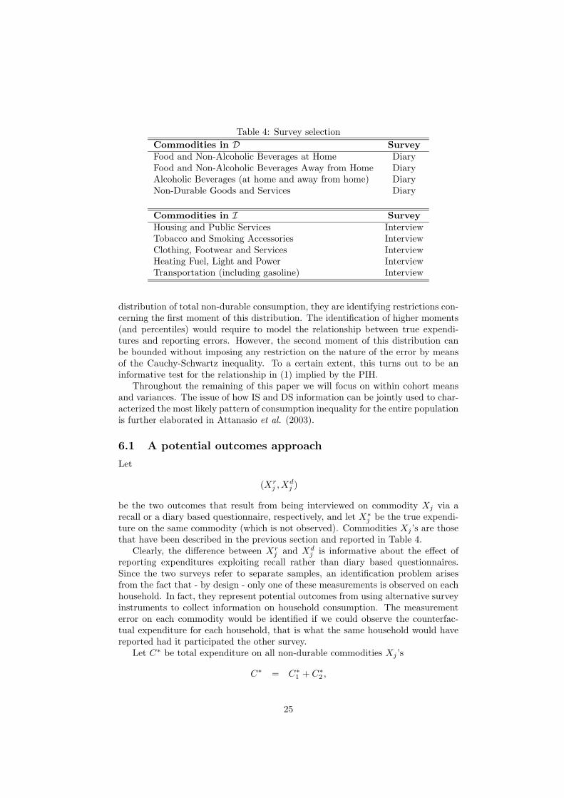
Table 4: Survey selectionCommodities in D SurveyFood and Non-Alcoholic Beverages at Home DiaryFood and Non-Alcoholic Beverages Away from Home DiaryAlcoholic Beverages (at home and away from home) DiaryNon-Durable Goods and Services Diary

Commodities in I SurveyHousing and Public Services InterviewTobacco and Smoking Accessories InterviewClothing, Footwear and Services InterviewHeating Fuel, Light and Power InterviewTransportation (including gasoline) Interview

distribution of total non-durable consumption, they are identifying restrictions con-cerning the first moment of this distribution. The identification of higher moments(and percentiles) would require to model the relationship between true expendi-tures and reporting errors. However, the second moment of this distribution canbe bounded without imposing any restriction on the nature of the error by meansof the Cauchy-Schwartz inequality. To a certain extent, this turns out to be aninformative test for the relationship in (1) implied by the PIH.

Throughout the remaining of this paper we will focus on within cohort meansand variances. The issue of how IS and DS information can be jointly used to char-acterized the most likely pattern of consumption inequality for the entire populationis further elaborated in Attanasio et al. (2003).

6.1 A potential outcomes approach

Let

(Xrj ,X

dj )

be the two outcomes that result from being interviewed on commodity Xj via arecall or a diary based questionnaire, respectively, and let X∗

j be the true expendi-ture on the same commodity (which is not observed). Commodities Xj ’s are thosethat have been described in the previous section and reported in Table 4.

Clearly, the difference between Xrj and Xd

j is informative about the effect ofreporting expenditures exploiting recall rather than diary based questionnaires.Since the two surveys refer to separate samples, an identification problem arisesfrom the fact that - by design - only one of these measurements is observed on eachhousehold. In fact, they represent potential outcomes from using alternative surveyinstruments to collect information on household consumption. The measurementerror on each commodity would be identified if we could observe the counterfac-tual expenditure for each household, that is what the same household would havereported had it participated the other survey.

Let C∗ be total expenditure on all non-durable commodities Xj ’s

C∗ = C∗1 + C∗

2 ,

25

where C∗1 and C∗

2 represent expenditure on commodities in I and in D, respectively,as defined by Table 4

C∗1 =

∑j∈I

X∗j , C∗

2 =∑j∈D

X∗j .

Total expenditure is not observable to the analyst. Rather two error affected mea-surements of C∗ are observed, representing the aggregate expenditures that resultfrom using IS or DS data

Cr = Cr1 + Cr

2 ,

Cd = Cd1 + Cd

2 ,

where (Cr1 , C

d1 ) and (Cr

2 , Cd2 ) are IS and DS expenditures on commodities in I and

in DCr

1 =∑j∈I

Xrj , Cr

2 =∑j∈D

Xrj ,

Cd1 =

∑j∈I

Xdj , Cd

2 =∑j∈D

Xdj .

By means of Conditions 1 and 2, the measurement error affecting the aggregateexpenditures Cr and Cd depends on the measurement error on different subsets ofcommodities entering total non-durable expenditure (i.e. those commodities eitherin D or in I, respectively). That is, total expenditure from IS data can be writtenas

Cr = C∗1 + Cr

2 ,

where the last expression follows since expenditures on commodities in I are notaffected by measurement error by assumption (Xr

j = X∗j ,∀j ∈ I). By analogy, it

follows that

Cd = Cd1 + C∗

2 ,

since Xdj = X∗

j ,∀j ∈ D. Accordingly, the error due to recall and diary interviewscan be written as

εr = Cr2 − C∗

2 , (3)εd = Cd

1 − C∗1 , (4)

respectively. Any difference in the distribution of these errors over time is respon-sible for the different pattern of means and variances observed in raw IS and DSdata.

The main points arising from the last two expressions can be summarized asfollows. Firstly, the mean of the IS (DS) error can be written as a linear combinationof means of errors for commodities in D (I, respectively). Since error means on allnon-durable commodities are identifiable because of Conditions 1 and 2, the meanvalues of (3) and (4) are identified by

E(εr) = E(Cr2)− E(Cd

2 ), (5)E(εd) = E(Cd

1 )− E(Cr1), (6)

26

born 1960−69

700

750

800

850

900

born 1950−59

born 1940−49

86 88 90 92 94 96 98 100102

700

750

800

850

900

born 1930−39

86 88 90 92 94 96 98 100102

Figure 6: Mean of family expenditure on non-durable goods by cohort after correc-tion (2001 dollars)

respectively. Accordingly, Conditions 1 and 2 are identifying restrictions concerningthe first moment of the distribution of total non-durable consumption (see Section6.2).

Secondly, recall and diary errors are likely to be correlated with C∗, since theydepend on a common set of commodities. This implies that the difference betweenthe real variance of consumption and the observed values of this variance in ISand DS data depends on the variance of the terms in (3) and (4) and on theircorrelation with C∗, which are not observable. Therefore the variance of C∗ cannotbe estimated without imposing additional restrictions on the error structure (seeSection 6.3).

6.2 Consumption levels

Differences in mean expenditure values for all commodities entering total non-durable expenditure have been already discussed in Section 4.1 (see also FiguresA.2-A.10 in the Appendix). By means of Conditions 1 and 2, they can be inter-preted as the effect of collecting expenditure information using the less appropriatemethodology, depending on whether the considered commodity belongs to D or I.

Mean aggregate errors for IS and DS data (that is the quantities in (5) and (6),respectively) are presented in Table 5, separately by cohort and over time. Moreprecisely, figures for IS and DS errors as proportion of total non-durable expenditureare reported, that is

E(εr)/E(C∗) E(εd)/E(C∗)

27

Table 5: Survey errors as a proportion of total non-durable expenditureyear born 1960-69 born 1950-59 born 1940-49 born 1930-39 all

IS DS IS DS IS DS IS DS IS DS1986 -0.05 -0.12 -0.03 -0.10 -0.01 -0.10 -0.02 -0.11 -0.02 -0.111987 0.02 -0.11 -0.02 -0.11 -0.03 -0.09 -0.01 -0.08 -0.01 -0.101988 -0.05 -0.09 -0.06 -0.10 -0.05 -0.08 -0.04 -0.08 -0.05 -0.091989 -0.07 -0.07 -0.05 -0.10 -0.05 -0.10 -0.07 -0.06 -0.06 -0.081990 -0.02 -0.06 -0.07 -0.09 -0.06 -0.06 -0.07 -0.05 -0.06 -0.071991 -0.03 -0.06 -0.08 -0.03 -0.07 -0.05 -0.06 -0.06 -0.06 -0.051992 -0.09 -0.04 -0.08 -0.05 -0.05 -0.08 -0.03 -0.04 -0.07 -0.051993 -0.07 -0.03 -0.05 -0.05 -0.06 -0.05 -0.06 -0.03 -0.06 -0.041994 -0.06 -0.04 -0.05 -0.03 -0.03 -0.05 -0.04 0.01 -0.04 -0.031995 -0.04 -0.06 -0.07 -0.03 -0.07 -0.02 -0.08 0.02 -0.06 -0.021996 -0.05 -0.02 -0.06 -0.05 -0.07 -0.04 -0.08 0.02 -0.06 -0.031997 -0.05 -0.02 -0.04 -0.03 -0.06 -0.01 -0.07 -0.06 -0.05 -0.031998 -0.07 -0.06 -0.08 -0.01 -0.04 -0.08 -0.06 -0.02 -0.06 -0.041999 -0.08 -0.03 -0.07 -0.06 -0.06 -0.06 -0.05 -0.04 -0.06 -0.052000 -0.07 -0.05 -0.08 -0.02 -0.04 -0.04 -0.08 -0.05 -0.07 -0.042001 -0.08 -0.05 -0.07 -0.01 -0.08 -0.02 -0.10 -0.06 -0.08 -0.03

28

respectively, where the mean of total expenditure is estimated by

E(C∗) = E(C∗1 ) + E(C∗

2 )= E(Cr

1) + E(Cd2 ). (7)

Negative (positive) numbers in the table can be interpreted as the proportion ofexpenditure under (over) reported in the IS or in the DS. Apparently, this propor-tion varies across cohorts, with younger cohorts more likely to have higher errorsthan older cohorts, both in the IS and in the DS. The amount of misreporting hasan almost stationary distribution over time for the IS, while it varies for the DS.In particular, the DS appears to become more accurate over time.17

Figure 6 presents estimated mean expenditures by cohort using (7) and can becompared to the results presented in Figure 2. It is evident that, even after thecorrection, consumption profiles are still sharply decreasing during the first half ofthe 1990s.18

6.3 Consumption inequality

The goal of this section is to derive the analogue of Figure 4 once the effect ofreporting errors is accounted for. Throughout our analysis, we will consider figuresfor the squared coefficient of variation of total expenditure instead of figures for thevariance of logs. The reason for this choice will be clear from what follows.

The variance of total expenditure can be expressed as a function of the varianceof commodities in D and I and between-group covariances

V ar(C∗) = V ar(C∗1 ) + V ar(C∗

2 ) + 2Cov(C∗1 , C

∗2 ). (8)

The ratio of the previous quantity to the squared mean of total consumption repre-sents a first order approximation for the variance of log consumption.19 Conditions1 and 2 are identifying restrictions only for the first two terms of the previousexpression, using either IS or DS data. On the other hand, the covariance termcannot be identified from the available information since by definition D ∩ I = ∅

17Given the restrictions imposed so far, the measurement error affecting the reporting of non-durable commodities cannot be further characterized. If we observed both recall and diary out-comes for commodity X on the same household, according to Condition 1 and Condition 2 theerror on that commodity would be (non-parametrically) identified. In fact, by writing

ξ = x − x∗,

we could identify the distribution of ξ by taking the difference between observed diary and recalloutcomes depending on the rule discussed in Table 4. In our case, although the first momentof this distribution can be easily recovered, the identification of higher moments and percentileswould require to know the structure of correlation between x and x∗, which is not observable.

18Following the same lines of the previous footnote, it can be shown that the distribution of C∗is not identified. Additional restrictions are required. Alternatively, bounds on this distributioncould be derived exploiting Frechet’s or Markov’s inequalities.

19A Taylor expansion of lnC∗ in a neighborhood of its mean gives

lnC∗ = lnE(C∗) +C∗ − E(C∗)

E(C∗)− [C∗ − E(C∗)]2

2E(C∗)2+ error,

so that the variance of logs is approximated by taking the squared coefficient of variation

V ar(C∗)E(C∗)2

= CV (C∗)2 � V ar(lnC∗).

29

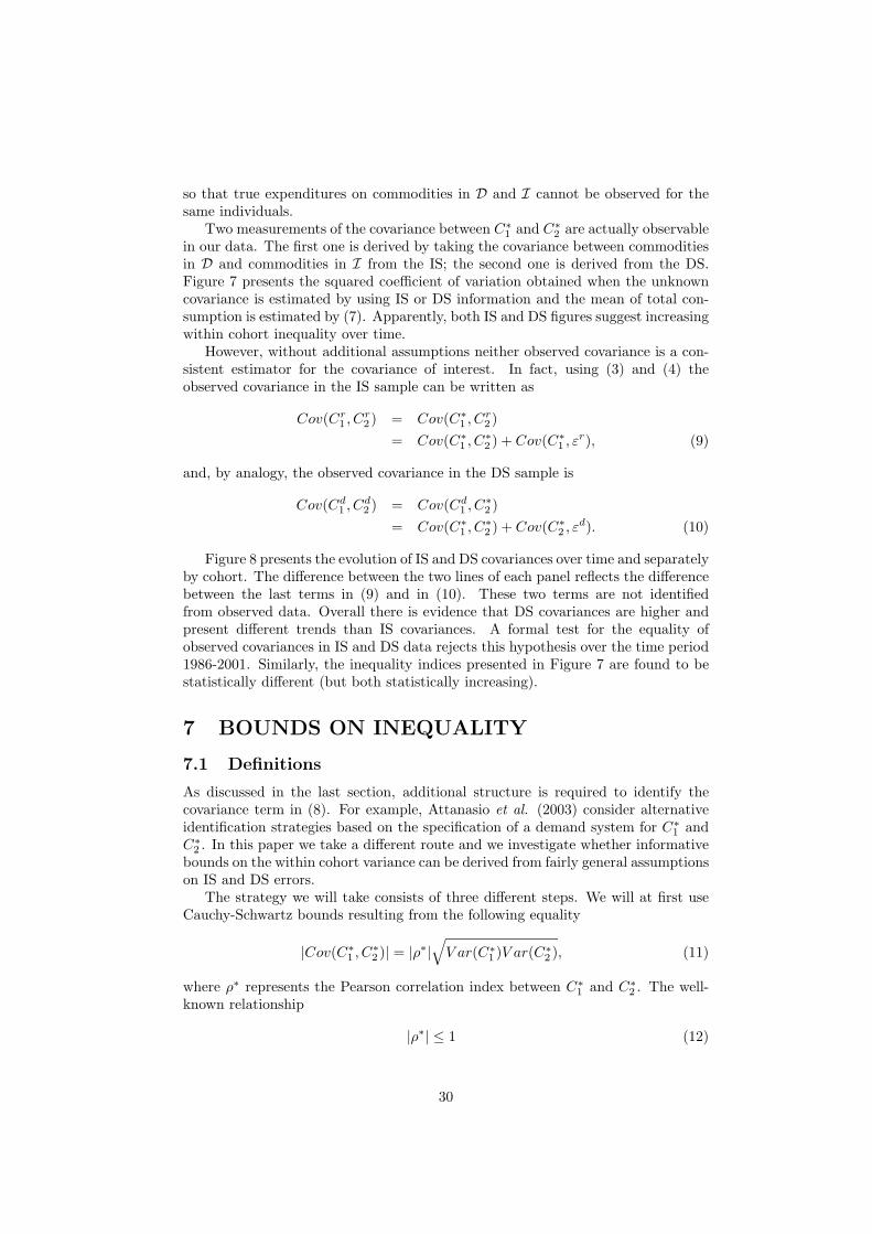
so that true expenditures on commodities in D and I cannot be observed for thesame individuals.

Two measurements of the covariance between C∗1 and C∗

2 are actually observablein our data. The first one is derived by taking the covariance between commoditiesin D and commodities in I from the IS; the second one is derived from the DS.Figure 7 presents the squared coefficient of variation obtained when the unknowncovariance is estimated by using IS or DS information and the mean of total con-sumption is estimated by (7). Apparently, both IS and DS figures suggest increasingwithin cohort inequality over time.

However, without additional assumptions neither observed covariance is a con-sistent estimator for the covariance of interest. In fact, using (3) and (4) theobserved covariance in the IS sample can be written as

Cov(Cr1 , C

r2) = Cov(C∗

1 , Cr2)

= Cov(C∗1 , C

∗2 ) + Cov(C∗

1 , εr), (9)

and, by analogy, the observed covariance in the DS sample is

Cov(Cd1 , C

d2 ) = Cov(Cd

1 , C∗2 )

= Cov(C∗1 , C

∗2 ) + Cov(C∗

2 , εd). (10)

Figure 8 presents the evolution of IS and DS covariances over time and separatelyby cohort. The difference between the two lines of each panel reflects the differencebetween the last terms in (9) and in (10). These two terms are not identifiedfrom observed data. Overall there is evidence that DS covariances are higher andpresent different trends than IS covariances. A formal test for the equality ofobserved covariances in IS and DS data rejects this hypothesis over the time period1986-2001. Similarly, the inequality indices presented in Figure 7 are found to bestatistically different (but both statistically increasing).

7 BOUNDS ON INEQUALITY

7.1 Definitions

As discussed in the last section, additional structure is required to identify thecovariance term in (8). For example, Attanasio et al. (2003) consider alternativeidentification strategies based on the specification of a demand system for C∗

1 andC∗

2 . In this paper we take a different route and we investigate whether informativebounds on the within cohort variance can be derived from fairly general assumptionson IS and DS errors.

The strategy we will take consists of three different steps. We will at first useCauchy-Schwartz bounds resulting from the following equality

|Cov(C∗1 , C

∗2 )| = |ρ∗|

√V ar(C∗

1 )V ar(C∗2 ), (11)

where ρ∗ represents the Pearson correlation index between C∗1 and C∗

2 . The well-known relationship

|ρ∗| ≤ 1 (12)

30

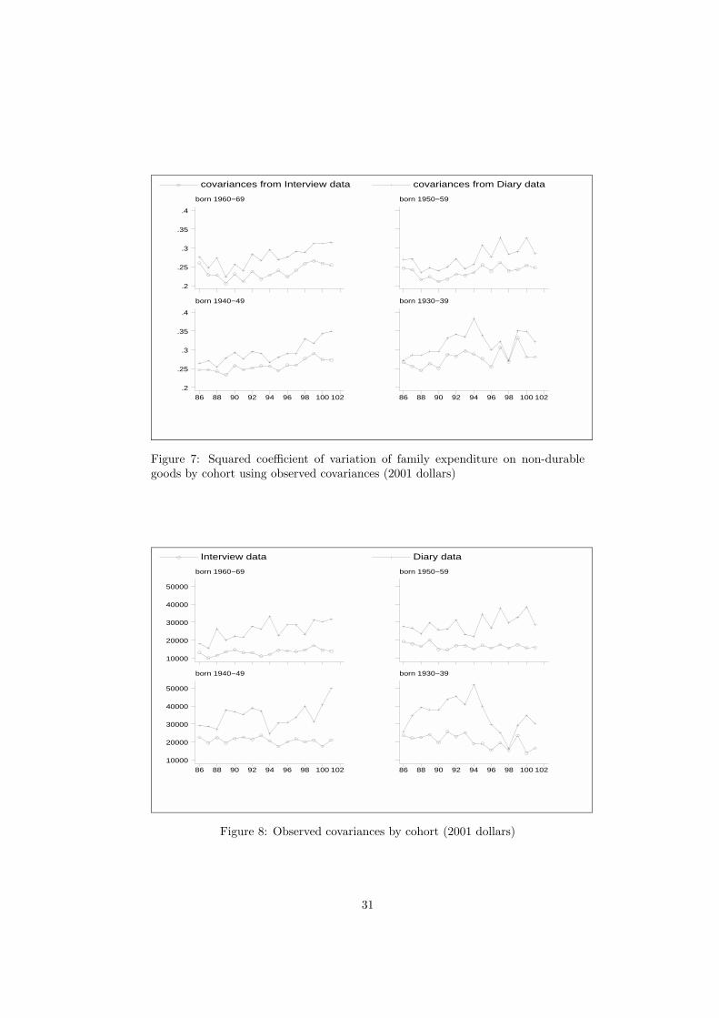
covariances from Interview data covariances from Diary data

born 1960−69

.2

.25

.3

.35

.4

born 1950−59

born 1940−49

86 88 90 92 94 96 98 100 102

.2

.25

.3

.35

.4

born 1930−39

86 88 90 92 94 96 98 100 102

Figure 7: Squared coefficient of variation of family expenditure on non-durablegoods by cohort using observed covariances (2001 dollars)

Interview data Diary data

born 1960−69

10000

20000

30000

40000

50000

born 1950−59

born 1940−49

86 88 90 92 94 96 98 100 102

10000

20000

30000

40000

50000

born 1930−39

86 88 90 92 94 96 98 100 102

Figure 8: Observed covariances by cohort (2001 dollars)

31

defines bounds for the within cohort covariance over time, since the product of thevariances in (11) is identifiable using the restrictions in Table 4.

However, although the interval [−1,+1] is often considered the reference rangefor evaluating the strength of empirical correlation, it is well known that the upperand the lower bounds can only be achieved if the marginal distributions of C∗

1

and C∗2 are linearly related (indeed, the Pearson coefficient detects only linear

correlation!). If the two distributions cannot be linearly related, the maximumattainable absolute correlation coefficient is lower than one (see for example thediscussion by Shih and Huang 1992).

More formally, let F ∗1 and F ∗

2 be the cumulative distribution functions of C∗1

and C∗2 , respectively, and let the corresponding inverse be defined as

F ∗−1j (t) = inf{x : F ∗

j (x) ≥ t}, j = 1, 2

for 0 ≤ t ≤ 1. Then the correlation between C∗1 and C∗

2 is bounded by

corr(F ∗−11 (W ), F ∗−1

2 (1−W )) ≤ ρ∗ ≤ corr(F ∗−11 (W ), F ∗−1

2 (W )), (13)

where W is a random variable distributed uniformly between zero and one. Notethat, if C∗

1 can be written as a linear function of C∗2 , then the previous expression

collapses to the Cauchy-Schwartz bound in (12).20 Bounds in (13) can be estimatedby taking the correlation between percentiles of the empirical distributions of C∗

1

and C∗2 which, by means of Conditions 1 and 2, are identified. They represent the

tightest bounds on the correlation coefficient attainable without imposing furtherrestrictions on the correlation of interest.

Bounds for the within cohort inequality resulting from this procedure are pre-sented in Figure 9. To assess the importance of sampling variability, figures frombootstrapped 95% confidence intervals will be discussed throughout this section.As expected, results are not informative on the pattern of within cohort inequalityover time.

Bounds in (13) can be improved by looking at the partial correlation betweenC∗

1 and C∗2 once a set of regressors Z is controlled for. The expression in (8) can be

written as the sum of the following within-group and between-group components

V ar(C∗) = EZV ar(C∗|Z) + V arZE(C∗|Z),which are defined as

V arZE(C∗|Z) = V arZ{E(C∗1 |Z) + E(C∗

2 |Z)},EZV ar(C∗|Z) = EZ{V ar(C∗

1 |Z) + V ar(C∗2 |Z) + 2Cov(C∗

1 , C∗2 |Z)},

where Z represents a set of family characteristics common across the two surveys.The first component is identified by assumption, since it represents the varianceacross groups defined by Z of total mean expenditure as it results from (7). Thesecond component is not identified because it contains the within group covariancebetween C∗

1 and C∗2 .

This covariance can be bounded along the same lines of what discussed above.To fix ideas, in what follows Z will represent total family income and householdswill be split into five mutually exclusive groups defined by income deciles (20% or

20Shih and Huang (1992) provide several examples where the bounds implied by (13) are verydifferent from the ‘natural’ bounds implied by (12).

32

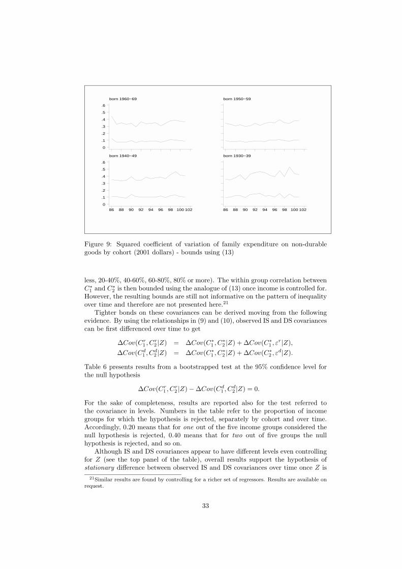
born 1960−69

0

.1

.2

.3

.4

.5

.6

born 1950−59

born 1940−49

86 88 90 92 94 96 98 100 102

0

.1

.2

.3

.4

.5

.6

born 1930−39

86 88 90 92 94 96 98 100 102

Figure 9: Squared coefficient of variation of family expenditure on non-durablegoods by cohort (2001 dollars) - bounds using (13)

less, 20-40%, 40-60%, 60-80%, 80% or more). The within group correlation betweenC∗

1 and C∗2 is then bounded using the analogue of (13) once income is controlled for.

However, the resulting bounds are still not informative on the pattern of inequalityover time and therefore are not presented here.21

Tighter bonds on these covariances can be derived moving from the followingevidence. By using the relationships in (9) and (10), observed IS and DS covariancescan be first differenced over time to get

∆Cov(Cr1 , C

r2 |Z) = ∆Cov(C∗

1 , C∗2 |Z) + ∆Cov(C∗

1 , εr|Z),

∆Cov(Cd1 , C

d2 |Z) = ∆Cov(C∗

1 , C∗2 |Z) + ∆Cov(C∗

2 , εd|Z).

Table 6 presents results from a bootstrapped test at the 95% confidence level forthe null hypothesis

∆Cov(Cr1 , C

r2 |Z)−∆Cov(Cd

1 , Cd2 |Z) = 0.

For the sake of completeness, results are reported also for the test referred tothe covariance in levels. Numbers in the table refer to the proportion of incomegroups for which the hypothesis is rejected, separately by cohort and over time.Accordingly, 0.20 means that for one out of the five income groups considered thenull hypothesis is rejected, 0.40 means that for two out of five groups the nullhypothesis is rejected, and so on.

Although IS and DS covariances appear to have different levels even controllingfor Z (see the top panel of the table), overall results support the hypothesis ofstationary difference between observed IS and DS covariances over time once Z is

21Similar results are found by controlling for a richer set of regressors. Results are available onrequest.

33

Table 6: Percentage of groups for which the null hypothesis is rejected

H0 : Cov(Cr1 , C

r2 |Z)− Cov(Cd

1 , Cd2 |Z) = 0

year born 1960-69 born 1950-59 born 1940-49 born 1930-391986 0.40 0.401987 0.60 0.401988 0.20 0.20 0.20 0.201989 0.20 0.40 0.401990 0.20 0.20 0.20 0.401991 0.80 0.401992 0.20 0.60 0.201993 0.20 0.40 0.20 0.401994 0.60 0.60 0.20 0.801995 0.60 0.80 0.20 0.201996 1.00 0.40 0.20 0.401997 0.40 0.40 0.60 0.201998 0.20 1.00 0.40 0.201999 0.80 1.00 0.40 0.202000 1.00 0.80 0.60 0.202001 1.00 0.60 0.80 0.20

H0 : ∆Cov(Cr1 , C

r2 |Z)−∆Cov(Cd

1 , Cd2 |Z) = 0

year born 1960-69 born 1950-59 born 1940-49 born 1930-391987 0.201988198919901991199219931994 0.201995199619971998199920002001 0.20

34

born 1960−69

0

.1

.2

.3

.4

.5

born 1950−59

born 1940−49

86 88 90 92 94 96 98 100 102

0

.1

.2

.3

.4

.5

born 1930−39

86 88 90 92 94 96 98 100 102

Figure 10: Squared coefficient of variation of family expenditure on non-durablegoods by cohort (2001 dollars) - bounds using (13) and Condition 3

controlled for. This represents a necessary condition for the following assumptionto be satisfied.

Condition 3. ∆Cov(C∗2 , ε

d|Z) = 0 and ∆Cov(C∗1 , ε

r|Z) = 0.

The previous assumption together with the bounds implied by (13) restricts therange of values of the partial covariance between C∗

1 and C∗2 given Z. Although the

level of the covariance of interest is unknown, the series of its changes over timeturns out to be identified by the series of variations in IS and DS data. Condition3 defines bounds on the inequality index over time. Technical details on how thesebounds are derived are presented in the Appendix.

Results are reported in Figure 10. Although Condition 3 turns out to be verypowerful in tightening the natural bounds implied by (13), it is not fully informativeon the pattern of within cohort inequality over time. Apparently, inequality growsover time for the cohort of those born in 1930-39 and for those born in 1930-39before 1993 (that is before the retirement age). Inequality for the two remainingcohorts (in particular for those born in 1950-59) is not statistically increasing atthe confidence level considered.

7.2 Discussion

A sensitivity analysis of these results with respect to the true value of the cor-relation coefficient ρ∗(Z) = corr(C∗

1 , C∗2 |Z) is presented in Figures 11-13. More

precisely, the same procedure described in the previous section is derived exploit-ing the additional assumption that the correlation between C∗

1 and C∗2 net of Z is

lower than 0.90, 0.85 and 0.80 in absolute value.

35

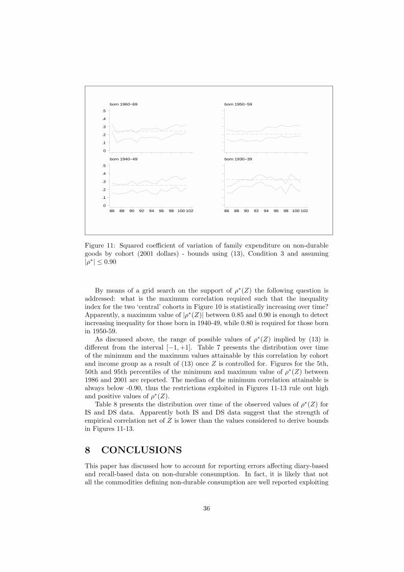
born 1960−69

0

.1

.2

.3

.4

.5

born 1950−59

born 1940−49

86 88 90 92 94 96 98 100 102

0

.1

.2

.3

.4

.5

born 1930−39

86 88 90 92 94 96 98 100 102

Figure 11: Squared coefficient of variation of family expenditure on non-durablegoods by cohort (2001 dollars) - bounds using (13), Condition 3 and assuming|ρ∗| ≤ 0.90

By means of a grid search on the support of ρ∗(Z) the following question isaddressed: what is the maximum correlation required such that the inequalityindex for the two ‘central’ cohorts in Figure 10 is statistically increasing over time?Apparently, a maximum value of |ρ∗(Z)| between 0.85 and 0.90 is enough to detectincreasing inequality for those born in 1940-49, while 0.80 is required for those bornin 1950-59.

As discussed above, the range of possible values of ρ∗(Z) implied by (13) isdifferent from the interval [−1,+1]. Table 7 presents the distribution over timeof the minimum and the maximum values attainable by this correlation by cohortand income group as a result of (13) once Z is controlled for. Figures for the 5th,50th and 95th percentiles of the minimum and maximum value of ρ∗(Z) between1986 and 2001 are reported. The median of the minimum correlation attainable isalways below -0.90, thus the restrictions exploited in Figures 11-13 rule out highand positive values of ρ∗(Z).

Table 8 presents the distribution over time of the observed values of ρ∗(Z) forIS and DS data. Apparently both IS and DS data suggest that the strength ofempirical correlation net of Z is lower than the values considered to derive boundsin Figures 11-13.

8 CONCLUSIONS

This paper has discussed how to account for reporting errors affecting diary-basedand recall-based data on non-durable consumption. In fact, it is likely that notall the commodities defining non-durable consumption are well reported exploiting

36

Table 7: Bounds implied by (13)income group born 1960-69 born 1950-59 born 1940-49 born 1930-39

min max min max min max min max0-20% 5% -0.88 0.91 -0.87 0.98 -0.91 0.92 -0.86 0.96

50% -0.81 0.99 -0.81 0.99 -0.78 0.99 -0.76 0.9895% -0.70 1.00 -0.76 1.00 -0.65 1.00 -0.68 1.00

20-40% 5% -0.93 0.96 -0.94 0.98 -0.90 0.98 -0.92 0.9650% -0.89 0.99 -0.90 0.99 -0.85 0.99 -0.82 0.9895% -0.77 1.00 -0.83 1.00 -0.78 1.00 -0.67 1.00

40-60% 5% -0.95 0.97 -0.96 0.98 -0.95 0.98 -0.93 0.9350% -0.90 0.99 -0.90 0.99 -0.90 0.99 -0.85 0.9895% -0.81 1.00 -0.87 1.00 -0.84 1.00 -0.76 0.99

60-80% 5% -0.94 0.97 -0.96 0.97 -0.95 0.96 -0.92 0.9750% -0.89 0.99 -0.91 0.99 -0.88 0.99 -0.86 0.9895% -0.83 1.00 -0.87 1.00 -0.81 1.00 -0.76 0.99

80-100% 5% -0.95 0.95 -0.89 0.98 -0.91 0.97 -0.89 0.9550% -0.87 0.99 -0.85 0.99 -0.83 0.99 -0.81 0.9895% -0.82 1.00 -0.79 1.00 -0.78 1.00 -0.65 0.99

37

Table 8: Observed correlationsincome group born 1960-69 born 1950-59 born 1940-49 born 1930-39

IS DS IS DS IS DS IS DS0-20% 5% 0.34 0.26 0.39 0.46 0.41 0.51 0.42 0.45

50% 0.42 0.51 0.46 0.61 0.48 0.56 0.50 0.5895% 0.51 0.68 0.52 0.71 0.57 0.66 0.63 0.71

20-40% 5% 0.23 0.22 0.35 0.39 0.28 0.28 0.26 0.3150% 0.39 0.50 0.44 0.48 0.42 0.53 0.38 0.4695% 0.49 0.73 0.48 0.60 0.54 0.63 0.45 0.68

40-60% 5% 0.11 0.19 0.28 0.38 0.23 0.21 0.26 0.2750% 0.30 0.43 0.34 0.46 0.36 0.49 0.37 0.4795% 0.41 0.58 0.40 0.61 0.44 0.57 0.45 0.61

60-80% 5% 0.14 0.25 0.19 0.33 0.23 0.27 0.17 0.3050% 0.27 0.42 0.34 0.46 0.32 0.43 0.31 0.4395% 0.35 0.51 0.38 0.58 0.44 0.67 0.35 0.64

80-100% 5% 0.18 0.18 0.23 0.25 0.23 0.28 0.26 0.2550% 0.29 0.37 0.33 0.40 0.30 0.46 0.39 0.4595% 0.40 0.55 0.42 0.56 0.39 0.55 0.46 0.66

38

born 1960−69

0

.1

.2

.3

.4

.5

born 1950−59

born 1940−49

86 88 90 92 94 96 98 100 102

0

.1

.2

.3

.4

.5

born 1930−39

86 88 90 92 94 96 98 100 102

Figure 12: Squared coefficient of variation of family expenditure on non-durablegoods by cohort (2001 dollars) - bounds using (13), Condition 3 and assuming|ρ∗| ≤ 0.85

born 1960−69

0

.1

.2

.3

.4

.5

born 1950−59

born 1940−49

86 88 90 92 94 96 98 100 102

0

.1

.2

.3

.4

.5

born 1930−39

86 88 90 92 94 96 98 100 102

Figure 13: Squared coefficient of variation of family expenditure on non-durablegoods by cohort (2001 dollars) - bounds using (13), Condition 3 and assuming|ρ∗| ≤ 0.80

39

only one of these two survey methodologies. Expenditures on frequently purchased,smaller items are presumably more accurate using diaries while recall data are moreappropriate for large expenditures or expenditures occurring on a regular basis.

It turns out that neither diary nor recall-based data alone provide a reliableaggregate measure of total expenditure on non-durables. One might argue that forany practical purpose these alternative data collection strategies lead to consistentresults in the estimation of economic models of consumption behavior. Unfortu-nately, evidence from the literature suggests that data themselves might not besuitable to validate existing models and that conclusions are strongly related to theinformation being used.

This issue has been addressed by looking at micro data from two independentsamples of households from the Consumer Expenditure Survey for the Unites States.This survey represent a unique source of data because it consists of diary an re-call information collected on the same set of items, although it refers to separatesamples of households. The integration of these datasets presents the problem ofdetermining the appropriate survey component from which to select expenditureitems. On the basis on evidence reported in a number of previous studies, we havesplit the set of commodities entering non-durable consumption into two groups in-dicating which one of the two survey methodologies (diary or recall) leads to moreaccurate data quality.

The comparison of the two surveys based on the overlap in coverage of expendi-tures offers insights for the effects of collection modes on data quality. Estimatingthe true expenditure level on frequently purchased items for the recall sample (andon bulky items in the diary sample) can be seen as a problem of inferring counter-factuals: what is the counterfactual diary (recall) expenditure measure for recall(diary) respondents?

We have shown that the pictures emerging from the two surveys are very dif-ferent, both with respect to mean expenditure and, more importantly, with respectto indices of inequality. More precisely, while the differences in mean expenditureare roughly constant over time, consumption inequality presents different levels andtrends in the two surveys. We have reconciled this evidence using integrated diaryand recall information to characterize the most likely pattern of consumption forcohorts of individuals defined by their age.

This procedure allows us (i) to define an improved measure for mean and vari-ance of non-durable expenditure over the 1990s and (ii) to characterize the mea-surement error affecting the commodities whose quality is doubtful according toother studies in the literature. The implications of our findings for the estimationof inequality indices have been discussed, with an application to permanent incomemodels. In particular, we have shown that using diary and recall data to improvethe quality of household consumption the permanent income hypothesis cannot berejected.

One general lesson can be deducted from this paper. Surveys are large measure-ment machines where many points might influence the ultimate error distribution.The collection of consumption data may be better structured as a set of overlap-ping questionnaires asking about only a small subset of consumption (as for theFamily Expenditure Survey for the United Kingdom). In this way, more accu-rate information on different components of consumption would be obtained by themost appropriate survey methodology. Moreover, information from diary and recallquestions collected for the same individuals would permit to shed more light intothe effects of collection modes on the quality of available information. The evidence

40

on this point currently available in the literature is very much limited to a smallgroups of commodities (mainly food).

References

[1] Atkinson, A. B., Gomulka, J., and Stern, N.H. (1990), “Spending on Alco-hol: Evidence from the Family Expenditure Survey 1970-1983,” The EconomicJournal, 100, 402, 808-827.

[2] Attanasio, O.P., Battistin, E. and Ichimura, H. (2003), unpublishedmanuscript, University College London.

[3] Attanasio, O.P., and Weber, G. (1995), “Is Consumption Growth Consistentwith Intertemporal Optimization? Evidence from the Consumer ExpenditureSurvey,” Journal of Political Economy, 103, 95, 1121-1157.

[4] Banks, J., and Johnson, P. (eds.) (1998), How Reliable is the Family Expen-diture Survey? Trends in Incomes and Expenditures over Time, London: TheInstitute for Fiscal Studies.

[5] Battistin, E. (2002), “Measurement error issues in modelling economic be-haviours - four case studies,” Ph.D thesis in Statistics, University of Padova.

[6] Battistin, E., Miniaci, R., and Weber, G. (2003), “What do we learn fromrecall consumption data?,” forthcoming Journal of Human Resources, 38, 2.

[7] Blundell, R., and Lewbel, A. (1999), “Puzzles of consumption and incomedistribution explained: Gibrat’s law for permanent income,” unpublishedmanuscript.

[8] Blundell, R., Pistaferri, L., and Preston, I. (2002), “Partial insurance, informa-tion and consumption dynamics,” working paper W02/16, Institute for FiscalStudies, London.

[9] Bound, J. Brown, C. and Mathiowetz, N. (2001), “Measurement error in surveydata,” in Handbook of Econometrics, eds. Heckman, J.J., and Leamer, E.,Volume 5, 3707-3843.

[10] Branch, R., and Jayasuriya, B. (1997), “Consumer Expenditure Interview andDiary Survey Data Selection: a New Method,” unpublished manuscript, Bu-reau of Labor Statistics.

[11] Browning, M. and Lusardi, A. (1996), “Household Saving: Micro Theories andMicro Facts,” Journal of Economic Literature, XXXIV, December, 1797-1855.

[12] Browning, M., Crossley, T.F., and Weber, G. (2002), “Asking ConsumptionQuestions in General Purpose Surveys,” unpublished manuscript.

[13] Bureau of Labor Statistics (2002), Handbook of Methods, Chapter 16, Con-sumer Expenditures and Income, available at www.bls.gov.

[14] Chesher, A., and Schluter, C. (2001), “Welfare measurement and measurementerror,” forthcoming Review of Economic Studies.

41

[15] Costa, D.L. (2001), “Estimating Real Income in the United States from 1888 to1994: Correcting CPI Bias Using Engel Curves,” Journal of Political Economy,109, 6, 1288-1310

[16] Deaton, A. (1992), Understanding Consumption, Oxford: Clarendon.

[17] Deaton, A., and Paxson, C. (1994), “Intertemporal Choice and Inequality,”Journal of Political Economy, 102, 3, 437-467.

[18] Deaton, A. and Paxson, C. (2000), “Growth and savings among individualsand households,” The Review of Economics and Statistics, 82, 2, 212-225.

[19] Garner, T.I. (1993), “Consumer Expenditures and Inequality: An AnalysisBased on Decomposition of the Gini Coefficient,” The Review of Economicsand Statistics, 75, 1, 134-138.

[20] Gieseman, R. (1987), “The Consumer Expenditure Survey: Quality Controlby Comparative Analysis,” Monthly Labor Review, March, 8-14.

[21] Hall, R.E. (1978), “Stochastic Implications of the Life Cycle-Permanent In-come Hypothesis: Theory and Evidence,” Journal of Political Economy, 86, 6,971-987.

[22] Hausman, J., Newey, W.K., and Powell, J. L. (1995), “Nonlinear Errors inVariables: Estimation of Some Engel Curves,” Journal of Econometrics, 65, 1,205-233.

[23] Johnson, D., and Shipp, S. (1995), “Trends In Inequality Using ConsumerExpenditures: 1960 To 1993,” BLS Economic Working Paper Series.

[24] Krueger, D., and Perri, F. (2001), “Does Income Inequality Lead to Con-sumption Inequality? Empirical Findings and a Theoretical Explanation,”unpublished manuscript.

[25] Lee, L., and Sepanski, J.H. (1995) “Consistent estimation of linear and non-linear errors-in-variables models with validation information,” Journal of theAmerican Statistical Association, 90, 429, 130-140.

[26] Lewbel, A. (1996), “Demand Estimation with Expenditure Measurement Er-rors on the Left and Right Hand Side,” Review of Economics and Statistics,78, 4, 718-725.

[27] Lusardi, A. (1996), “Permanent Income, Current Income and Consumption:Evidence from Two Panel Data Sets,” Journal of Business and EconomicStatistics, 14, 1, 81-90.

[28] Lyberg, L., Biemer, P., Collins, M., de Leeuw, E., Dippo, C., Schwarz, N., andTrewin, D. (eds.) (1997), Survey Measurement and Process Quality, New York:Wiley.

[29] McCarthy, M., Johnson, D., Garner, T., and Passero, B. (2002), “Issues inConstruction and Research Use of the Consumer Expenditure Survey,” paperpresented at the 2002 NBER Summer Institute.

42

[30] Neter, J., and Waksberg, J. (1964), “A Study of Response Errors in Expen-ditures Data from Household Interviews,” Journal of the American StatisticalAssociation, 59, 305, 18-55.

[31] Pischke, J.S. (1995), “Measurement Error and Earnings Dynamics: Some Es-timates from the PSID Validation Study,” Journal of Business and EconomicStatistics, 13, 3, 305-314.

[32] Poikolainen, K., and Karkkainen, P. (1983), “Diary Gives More Accurate Infor-mation About Alcohol Consumption than Questionnaire,” Drug and AlcoholDependence, 11, 209-216.

[33] Rodgers, W.L., Brown, C., and Duncan, G.J. (1993), “Errors in Survey Re-ports of Earnings, Hours Worked and Hourly Wages,” Journal of the AmericanStatistical Association, 88, 424, 1208-1218.

[34] Sabelhaus, J. (1996), “Consumer Expenditure Survey: Family-Level Extracts,1980:1-1994:1,” Congressional Budget Office, available at www.nber.org.

[35] Shih, W.J., and Huang, W.M. (1992), “Evaluating Correlation with ProperBounds Biometrics,” Biometrics, 48, 4, 1207-1213.

[36] Shorrocks, A.F. (1982), “Inequality Decomposition by Factor Components,”Econometrica, 50, 1, 193-211.

[37] Silberstein, A.R., and Jacobs, C.A. (1989), “Symptoms of Repeated InterviewEffects in the Consumer Expenditure Survey,” in Panel Surveys, eds. Kasprzyk,D., Duncan, G., Kalton, G., and Singh, M.P., New York: Wiley, 289-303.

[38] Silberstein, A.R., and Scott, S. (1991), “Expenditure Diary Surveys and TheirAssociated Errors,” in Measurement Errors in Surveys, eds. Biemer, P.P.,Groves, R.M., Lyberg, L.E., Mathiowetz, N.A., and Sudman, S., New York:Wiley, 303-326.

[39] Slesnick, D.T. (1998), “Are our Data Relevant to the Theory? The Case ofAggregate Consumption,” Journal of Business and Economic Statistics, 16, 1,52-61.

[40] Slesnick, D.T. (2001), Consumption and Social Welfare. Living Standards andTheir Distribution in the United Staes, Cambridge: Cambridge UniversityPress.

[41] Stanton, J.L., and Tucci, L.A. (1982), “The Measurement of Consumption: Acomparison of Surveys and Diaries,” Journal of Marketing Research, 19, 274-277.

[42] Torelli, N., and Trivellato, U. (1993), “Modelling Inaccuracies in Job-SearchDuration Data,” Journal of Econometrics, 59, 1/2, 187-211.

[43] Tucker, C. (1992), “The Estimation of Instrument Effects on Data Quality inthe Consumer Expenditure Survey,” Journal of Official Statistics, 8, 1, 41-61.

[44] Turner, R. (1961), “Inter- Week Variations in Expenditure Recorded During aTwo-Week Survey of Family Expenditure,” Applied Statistics, 10, 3, 136-146.

43

[45] Wilcox, D.W. (1992), “The Construction of U.S. Consumption Data: SomeFacts and Their Implications for Empirical work,” American Economic Review,82, 922-941.

[46] Winter, J.K. (2002), “Design effects in survey-based measures of householdconsumption,” unpublished manuscript.

[47] Ziliak, J.P. (1998), “Does the Choice of Consumption Measure Matter? AnApplication to the Permanent-Income Hypothesis,” Journal of Monetary Eco-nomics, 41, 1, 201-216.

44

TECHNICAL APPENDIX

Bounds on Cov(C∗1 , C

∗2 |Z) using Condition 3 presented in Section 7 are derived in

what follows. Let

ηt = Cov(C∗1 , C

∗2 |Z)

be the quantity of interest and let

η̃t = ηt − ηt−1

be its changes over time. It is assumed that ηt can vary between known values ltand ut defined by the Cauchy-Schwartz bounds. Moreover, η̃t is also identified byobserved changes in IS and DS covariances if Condition 3 holds true.

Let

st = {. . . , ηt − η̃t − η̃t−1, ηt − η̃t, ηt, ηt + η̃t+1, ηt + η̃t+1 + η̃t+2, . . . }

be the the time series of covariances given ηt. In light of Condition 3, such asequence would be fully determined if ηt were observed.

Let

St = {st : lt ≤ ηt ≤ ut}

the set of sequences st consistent with the assumption that ηt is bounded betweenlt and ut. The set

B =⋂t

St

defines all the sequences that jointly satisfy the Cauchy-Schwartz bounds over timeand are consistent with the time series of observed changes η̃t. This set representsthe basis to derive the bounds exploited in Figures 10-13.

I

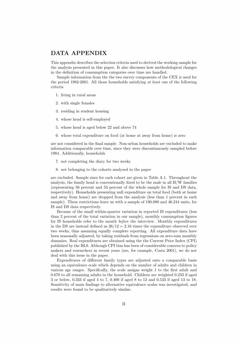
DATA APPENDIX

This appendix describes the selection criteria used to derived the working sample forthe analysis presented in this paper. It also discusses how methodological changesin the definition of consumption categories over time are handled.

Sample information from the the two survey components of the CEX is used forthe period 1982-2001. All those households satisfying at least one of the followingcriteria

1. living in rural areas

2. with single females

3. residing in student housing

4. whose head is self-employed

5. whose head is aged below 22 and above 74

6. whose total expenditure on food (at home at away from home) is zero

are not considered in the final sample. Non-urban households are excluded to makeinformation comparable over time, since they were discontinuously sampled before1984. Additionally, households

7. not completing the diary for two weeks

8. not belonging to the cohorts analyzed in the paper

are excluded. Sample sizes for each cohort are given in Table A.1. Throughout theanalysis, the family head is conventionally fixed to be the male in all H/W families(representing 56 percent and 53 percent of the whole sample for IS and DS data,respectively). Households presenting null expenditure on total food (both at homeand away from home) are dropped from the analysis (less than 1 percent in eachsample). These restrictions leave us with a sample of 190.080 and 46.244 units, forIS and DS data respectively.

Because of the small within-quarter variation in reported IS expenditures (lessthan 2 percent of the total variation in our sample), monthly consumption figuresfor IS households refer to the month before the interview. Monthly expendituresin the DS are instead defined as 26/12 = 2.16 times the expenditure observed overtwo weeks, thus assuming equally complete reporting. All expenditure data havebeen seasonally adjusted, by taking residuals from regressions on zero-sum monthlydummies. Real expenditures are obtained using the the Current Price Index (CPI)published by the BLS. Although CPI bias has been of considerable concern to policymakers and researchers in recent years (see, for example, Costa 2001), we do notdeal with this issue in the paper.

Expenditures of different family types are adjusted onto a comparable basisusing an equivalence scale which depends on the number of adults and children invarious age ranges. Specifically, the scale assigns weight 1 to the first adult and0.670 to all remaining adults in the household. Children are weighted 0.233 if aged3 or below, 0.333 if aged 4 to 7, 0.400 if aged 8 to 12 and 0.533 if aged 13 to 18.Sensitivity of main findings to alternative equivalence scales was investigated, andresults were found to be qualitatively similar.

II

Table A.1: Sample sizesDiary sample

year born 1960-69 born 1950-59 born 1940-49 born 1930-39 Totals1986 257 864 675 419 2,2151987 383 849 633 466 2,3311988 345 756 515 374 1,9901989 422 738 603 412 2,1751990 497 809 578 459 2,3431991 574 808 571 396 2,3491992 603 744 555 352 2,2541993 624 726 527 370 2,2471994 560 663 476 295 1,9941995 542 587 444 265 1,8381996 688 758 504 328 2,2781997 722 740 579 411 2,4521998 674 751 543 347 2,3151999 985 997 716 481 3,1792000 1,021 931 722 457 3,1312001 1,044 950 691 418 3,103

Interview sampleyear born 1960-69 born 1950-59 born 1940-49 born 1930-39 Totals1982 2,881 2,883 1,979 7,7431983 242 3,226 2,804 1,901 8,1731984 435 3,059 2,577 1,729 7,8001985 572 2,765 2,201 1,587 7,1251986 989 3,498 2,690 2,023 9,2001987 1,217 3,376 2,609 1,995 9,1971988 1,436 2,852 2,411 1,611 8,3101989 1,724 2,768 2,412 1,590 8,4941990 1,943 2,904 2,309 1,472 8,6281991 2,030 2,862 2,181 1,568 8,6411992 2,334 2,869 1,978 1,467 8,6481993 2,424 2,899 2,159 1,424 8,9061994 2,380 2,869 2,132 1,384 8,7651995 2,133 2,526 1,849 1,213 7,7211996 2,954 3,244 2,380 1,541 10,1191997 3,088 3,363 2,347 1,585 10,3831998 3,043 3,221 2,268 1,691 10,2231999 4,331 4,493 3,147 2,232 14,2032000 4,393 4,381 3,259 2,216 14,2492001 4,314 4,099 3,207 1,932 13,552

III

Table A.2: Definitions of expenditure categoriesCommodities in D Diary InterviewFood and Non-Alcoholic Beverages at Home 83-87Food and Non-Alcoholic Beverages Away from HomeAlcoholic Beverages (at home and away from home)Non-Durable Goods and Services 82-85

Newspapers and MagazinesNon-durable Entertainment ExpensesHousekeeping ServicesPersonal Care

Commodities in I Diary InterviewHousing and Public Services 82-85

Home Maintenance ServicesPublic UtilitiesMiscellaneous Home Services

Tobacco and Smoking AccessoriesClothing, Footwear and Services

Clothing, FootwearServices

Heating Fuel, Light and Power 82-85Transportation (including gasoline) 82-85

Fuel for TransportationTransportation Equipment Maintenance and RepairPublic TransportationVehicle Rental and Misc. Transportation Expenses

IV

80.1 82.1 84.1 86.1 88.1 90.1 92.1 94.1 96.1 98.1 100.1

5.7

5.8

5.9

6

6.1

Figure A.1: Logs of monthly Food at Home expenditure in 2000 dollars - InterviewSurvey

Detailed expenditure categories included in total non-durable consumption arereported in Table A.2. The top panel refers to those commodities labelled in thetext as D, while the bottom panel to commodities in I. The second and the thirdcolumns report the time intervals for which expenditure on non-durable commodi-ties cannot be directly derived from public use tapes because of definitional prob-lems, separately for IS and DS data. Accordingly, expenditures referring to “Hous-ing and Public Services” and “Non-durable Services” have been introduced in theDS only after 1986, with the exception of very few items for “Home MaintenanceServices” and “Non-durable Entertainment Expenses”. Similarly, information on“Fuel” and “Transportation” expenses is not available from public tapes between1982 and 1985.

As for IS data, the time series of food at home expenditure presents disconti-nuities introduced by changes in survey design in 1982 and 1987. In fact, recallinformation on food was derived in different ways over the years and the averagespending appears to be heavily affected by the exact wording, as shown in FigureA.1. Spikes downwards in 1982 and upwards in 1988 are the effect of asking re-spondents for usual spending on a monthly basis or on a weekly basis. In 1980-1981the question was on usual weekly expenditure on food over the past three months.In 1982-1987 the question was on how often and how much was spent in food overthe previous month. In 1988, the 1980-1981 question was resumed.

Discontinuities in levels are accounted for by running a regression of real foodexpenditure on a quadratic time trend and a time dummy for the period 1982-1987, a polynomial in family income and additional household controls. Reportedexpenditure are then scaled up for all households between 1982 and 1987 by thesame amount. Accordingly, the underlying assumption made is that changes inthe wording of food-related questions only affect the level of reporting, but not the

V

variance.Because of the definitional problems summarized in Table A.2, it follows that

total expenditure figures for IS and DS data are not fully comparable over time.For this reason, figures reported in the paper for total spending on non-durablesexploit 16 years of data for the DS (i.e. 1986-2001) and 20 years for the IS (i.e. 1982-2001). The aggregation rule suggested in Table 4 is therefore partially implementedover time. As a first approximation, only aggregate values of IS expenditures areconsidered before 1986, while integrated information for the DS is used after then.

The comparison of mean expenditure for the commodities defined in Table A.2is presented in Figures A.2-A.10. A detailed description of the items used to definethe categories of non-durable consumption can be downloaded at

http://www.stat.unipd.it/∼erich/papers.html,

separately for IS and DS data.Diary and recall information is available from the DS on expenditure for food

items. As noted earlier, food and non-alcoholic beverages is the only commodityentering non-durable expenditure for which recall and diary-based measurementson the same household are available. The information on the ‘usual’ spendingis collected for each household at the beginning of the (two-week) diary period.Therefore, its accuracy is presumably not influenced by how respondents learnabout own expenditures during the interview.

Figure A.11 presents the difference between weekly expenditure derived fromdiaries (as the sum of detailed food data) and weekly ‘usual’ expenditure for foodand non-alcoholic beverages at grocery stores given by respondents. As alreadypointed out by several papers using similar data sources, diary expenditure levelsin the first week tend to be higher that those for the second week. However,information from recall data leads to higher values of reported expenditures.1

It is worth noting that the difference between diary and recall figures condi-tional on the expenditure month (to control for seasonal effects) is always negativefor the period of time covered by this analysis, with values generally decreasing inabsolute value over time. There is a mild effect of the interview month on the mag-nitude of diary under reporting, since households interviewed in December usuallypresent values closer to zero. This evidence supports the idea that recall questionsoverstate the real spending on food-related items possibly because households’ re-porting includes more than just food-related goods. Indeed the recall questionabout food expenditure in the IS is derived subtracting to the usual amount spentat the grocery store the usual amount on non-food items.

1We found a very similar pattern comparing recall and diary information from the NationalFood Survey for the United Kingdom. Results are available on request.

VI

Interview data Diary data

born 1960−69

100

150

200

250

born 1950−59

born 1940−49

82 84 86 88 90 92 94 96 98 100102

100

150

200

250

born 1930−39

82 84 86 88 90 92 94 96 98 100102

Figure A.2: Mean of family expenditure on food and non-alcoholic beverages athome (2000 dollars)

Interview data Diary data

born 1960−69

50

100

150

born 1950−59

born 1940−49

82 84 86 88 90 92 94 96 98 100102

50

100

150

born 1930−39

82 84 86 88 90 92 94 96 98 100102

Figure A.3: Mean of family expenditure on food and non-alcoholic beverages awayfrom home (2000 dollars)

VII

Interview data Diary data

born 1960−69

10

20

30

40

50

born 1950−59

born 1940−49

82 84 86 88 90 92 94 96 98 100102

10

20

30

40

50

born 1930−39

82 84 86 88 90 92 94 96 98 100102

Figure A.4: Mean of family expenditure on alcoholic beverages (2000 dollars)

Interview data Diary data

born 1960−69

50

100

150

born 1950−59

born 1940−49

82 84 86 88 90 92 94 96 98 100102

50

100

150

born 1930−39

82 84 86 88 90 92 94 96 98 100102

Figure A.5: Mean of family expenditure on non-durable goods and services (2000dollars)

VIII

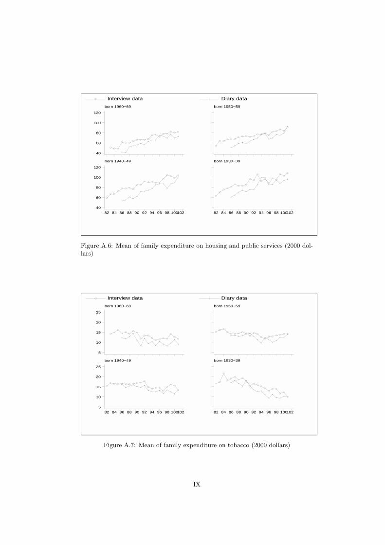
Interview data Diary data

born 1960−69

40

60

80

100

120

born 1950−59

born 1940−49

82 84 86 88 90 92 94 96 98 100102

40

60

80

100

120

born 1930−39

82 84 86 88 90 92 94 96 98 100102

Figure A.6: Mean of family expenditure on housing and public services (2000 dol-lars)

Interview data Diary data

born 1960−69

5

10

15

20

25

born 1950−59

born 1940−49

82 84 86 88 90 92 94 96 98 100102

5

10

15

20

25

born 1930−39

82 84 86 88 90 92 94 96 98 100102

Figure A.7: Mean of family expenditure on tobacco (2000 dollars)

IX

Interview data Diary data

born 1960−69

40

60

80

100

born 1950−59

born 1940−49

82 84 86 88 90 92 94 96 98 100102

40

60

80

100

born 1930−39

82 84 86 88 90 92 94 96 98 100102

Figure A.8: Mean of family expenditure on clothing, footwear and services (2000dollars)

Interview data Diary data

born 1960−69

40

50

60

70

80

born 1950−59

born 1940−49

82 84 86 88 90 92 94 96 98 100102

40

50

60

70

80

born 1930−39

82 84 86 88 90 92 94 96 98 100102

Figure A.9: Mean of family expenditure on heating fuel, light and power (2000dollars)

X

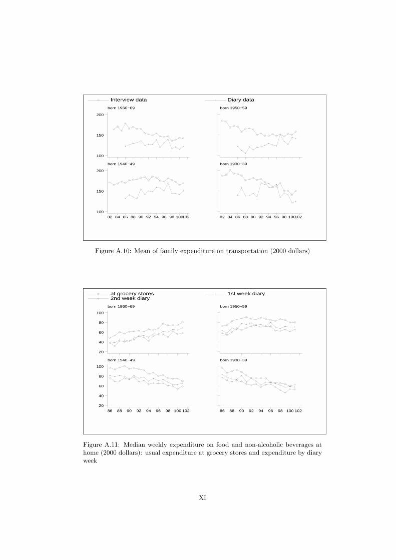
Interview data Diary data

born 1960−69

100

150

200

born 1950−59

born 1940−49

82 84 86 88 90 92 94 96 98 100102

100

150

200

born 1930−39

82 84 86 88 90 92 94 96 98 100102

Figure A.10: Mean of family expenditure on transportation (2000 dollars)

at grocery stores 1st week diary 2nd week diary

born 1960−69

20

40

60

80

100

born 1950−59

born 1940−49

86 88 90 92 94 96 98 100 102

20

40

60

80

100

born 1930−39

86 88 90 92 94 96 98 100 102

Figure A.11: Median weekly expenditure on food and non-alcoholic beverages athome (2000 dollars): usual expenditure at grocery stores and expenditure by diaryweek

XI

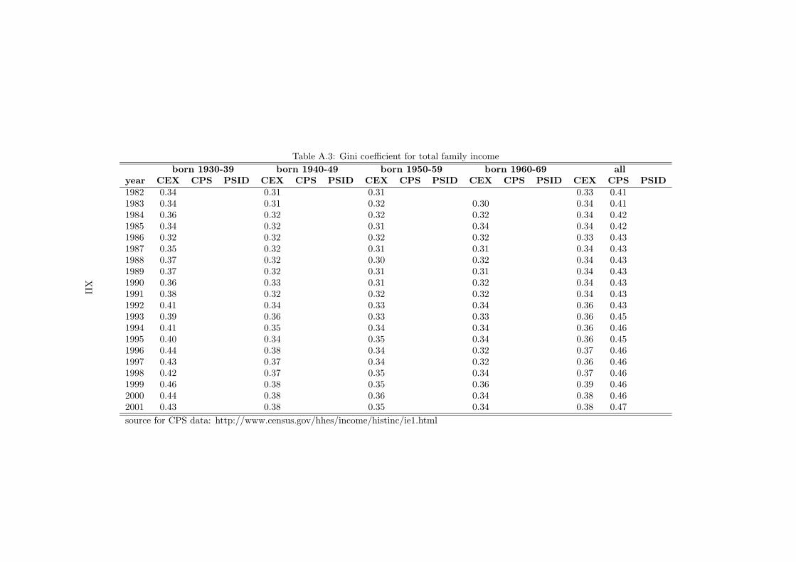
Table A.3: Gini coefficient for total family incomeborn 1930-39 born 1940-49 born 1950-59 born 1960-69 all

year CEX CPS PSID CEX CPS PSID CEX CPS PSID CEX CPS PSID CEX CPS PSID1982 0.34 0.31 0.31 0.33 0.411983 0.34 0.31 0.32 0.30 0.34 0.411984 0.36 0.32 0.32 0.32 0.34 0.421985 0.34 0.32 0.31 0.34 0.34 0.421986 0.32 0.32 0.32 0.32 0.33 0.431987 0.35 0.32 0.31 0.31 0.34 0.431988 0.37 0.32 0.30 0.32 0.34 0.431989 0.37 0.32 0.31 0.31 0.34 0.431990 0.36 0.33 0.31 0.32 0.34 0.431991 0.38 0.32 0.32 0.32 0.34 0.431992 0.41 0.34 0.33 0.34 0.36 0.431993 0.39 0.36 0.33 0.33 0.36 0.451994 0.41 0.35 0.34 0.34 0.36 0.461995 0.40 0.34 0.35 0.34 0.36 0.451996 0.44 0.38 0.34 0.32 0.37 0.461997 0.43 0.37 0.34 0.32 0.36 0.461998 0.42 0.37 0.35 0.34 0.37 0.461999 0.46 0.38 0.35 0.36 0.39 0.462000 0.44 0.38 0.36 0.34 0.38 0.462001 0.43 0.38 0.35 0.34 0.38 0.47source for CPS data: http://www.census.gov/hhes/income/histinc/ie1.html

XII

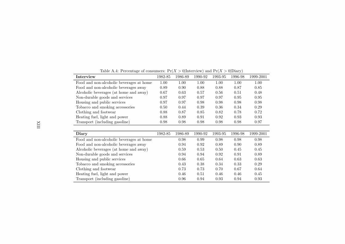
Table A.4: Percentage of consumers: Pr(X > 0|Interview) and Pr(X > 0|Diary)Interview 1982-85 1986-89 1990-92 1993-95 1996-98 1999-2001Food and non-alcoholic beverages at home 1.00 1.00 1.00 1.00 1.00 1.00Food and non-alcoholic beverages away 0.89 0.90 0.88 0.88 0.87 0.85Alcoholic beverages (at home and away) 0.67 0.63 0.57 0.56 0.51 0.48Non-durable goods and services 0.97 0.97 0.97 0.97 0.95 0.95Housing and public services 0.97 0.97 0.98 0.98 0.98 0.98Tobacco and smoking accessories 0.50 0.44 0.39 0.36 0.34 0.29Clothing and footwear 0.88 0.87 0.85 0.82 0.78 0.72Heating fuel, light and power 0.88 0.89 0.91 0.92 0.93 0.93Transport (including gasoline) 0.98 0.98 0.98 0.98 0.98 0.97

Diary 1982-85 1986-89 1990-92 1993-95 1996-98 1999-2001Food and non-alcoholic beverages at home 0.98 0.99 0.98 0.98 0.98Food and non-alcoholic beverages away 0.94 0.92 0.89 0.90 0.89Alcoholic beverages (at home and away) 0.59 0.53 0.50 0.45 0.45Non-durable goods and services 0.94 0.94 0.92 0.91 0.89Housing and public services 0.66 0.65 0.64 0.63 0.63Tobacco and smoking accessories 0.43 0.38 0.34 0.33 0.29Clothing and footwear 0.73 0.73 0.70 0.67 0.64Heating fuel, light and power 0.46 0.51 0.46 0.46 0.45Transport (including gasoline) 0.96 0.94 0.93 0.94 0.93

XIII