es159/259 ch. 4: velocity kinematics. es159/259 velocity kinematics we want to relate end-effector...
Post on 20-Dec-2015
222 views
TRANSCRIPT
ES159/259
Ch. 4: Velocity Kinematics
ES159/259
Velocity Kinematics
• We want to relate end-effector linear and angular velocities with the joint velocities
• First we will discuss angular velocities about a fixed axis
• Second we discuss angular velocities about arbitrary (moving) axes
• We will then introduce the Jacobian– Instantaneous transformation between a vector in Rn representing joint
velocities to a vector in R6 representing the linear and angular velocities of the end-effector
ES159/259
Angular velocity: arbitrary axis
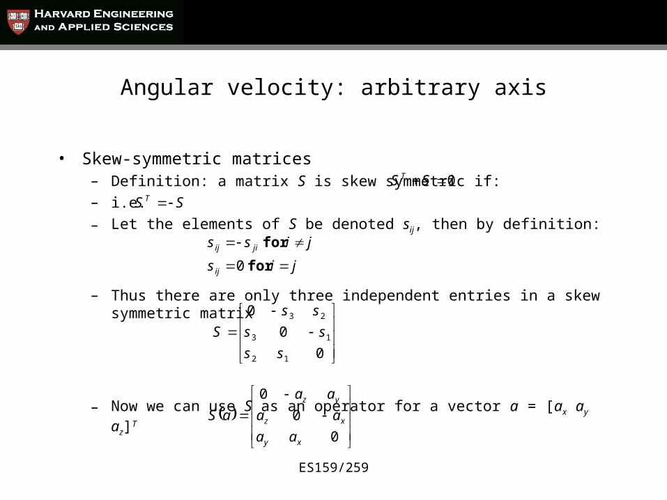
• Skew-symmetric matrices– Definition: a matrix S is skew symmetric if:– i.e.
– Let the elements of S be denoted sij, then by definition:
– Thus there are only three independent entries in a skew symmetric matrix
– Now we can use S as an operator for a vector a = [ax ay az]T
0SST
SST
jis
jiss
ij
jiij
for
for
0
0
0
0
12
13
23
ss
ss
ss
S
0
0
0
xy
xz
yz
aa
aa
aa
aS
ES159/259
Angular velocity: arbitrary axis
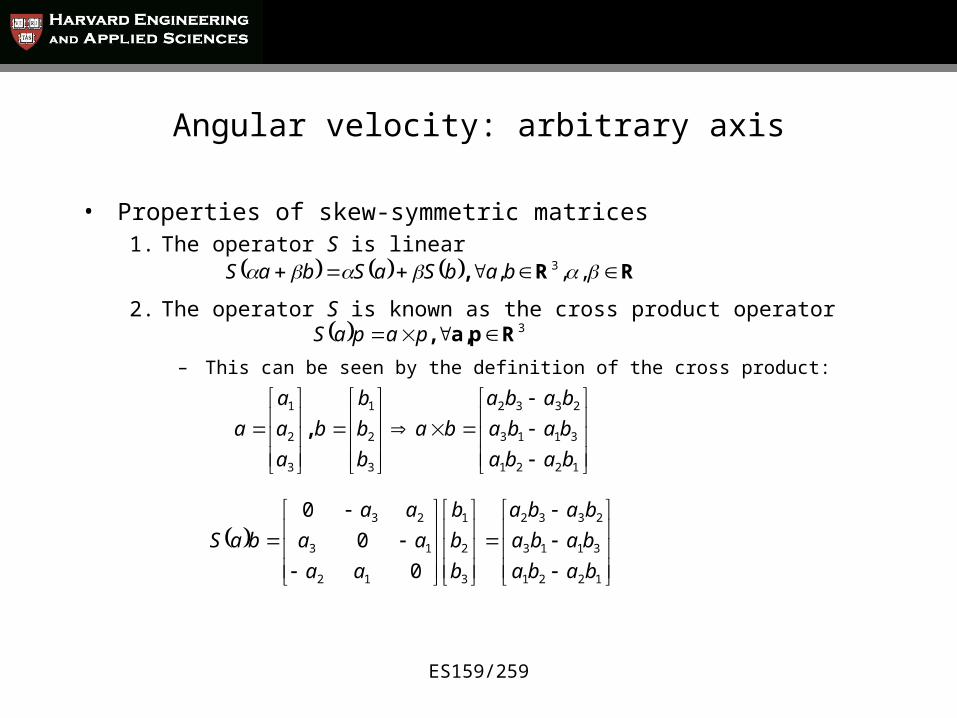
• Properties of skew-symmetric matrices 1. The operator S is linear
2. The operator S is known as the cross product operator
– This can be seen by the definition of the cross product:
RR , ,,, 3babSaSbaS
3Rpa, , papaS
1221
3113
2332
3
2
1
3
2
1
baba
baba
baba
ba
b
b
b
b
a
a
a
a ,
1221
3113
2332
3
2
1
12
13
23
0
0
0
baba
baba
baba
b
b
b
aa
aa
aa
baS

ES159/259
Angular velocity: arbitrary axis
• Properties of skew-symmetric matrices 3. For
– This can be shown for and R as follows:
– This can be shown by direct calculation. Finally:
4. For any
33 R , aSOR
33 SORa,bRbRabaR ,R ,
RaSRaRS T
bRaS
bRa
bRRRa
bRaRbRaRST
TT
nxnsoS R ,
0SxxT

ES159/259
Angular velocity: arbitrary axis
• Derivative of a rotation matrix – let R be an arbitrary rotation matrix which is a function of a single variable
• R()R()T=I
• Differentiating both sides (w/ respect to ) gives:
• Now define the matrix S as:
• Then ST is:
• Therefore S + ST = 0 and
0
TT R
d
dRRR
d
d
TRRd
dS
T
TTT R
d
dRRR
d
dS
Rd
dRRR
d
dSR T

ES159/259
Angular velocity: arbitrary axis
• Example: let R=Rx,, then using the previous results we have:
iS
RRd
dS T
ˆ
010
100
000
cossin0
sincos0
001
sincos0
cossin0
000
ES159/259
Angular velocity: arbitrary axis
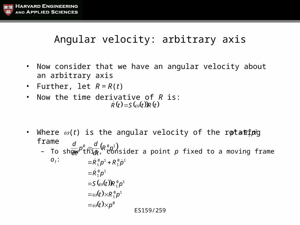
• Now consider that we have an angular velocity about an arbitrary axis
• Further, let R = R(t)
• Now the time derivative of R is:
• Where (t) is the angular velocity of the rotating frame– To show this, consider a point p fixed to a moving frame o1:
tRtStR
101
0 pRp
0
101
101
101
101
101
101
0
pt
pRt
pRtS
pR
pRpR
pRdt
dp
dt
d
ES159/259
Addition of angular velocities
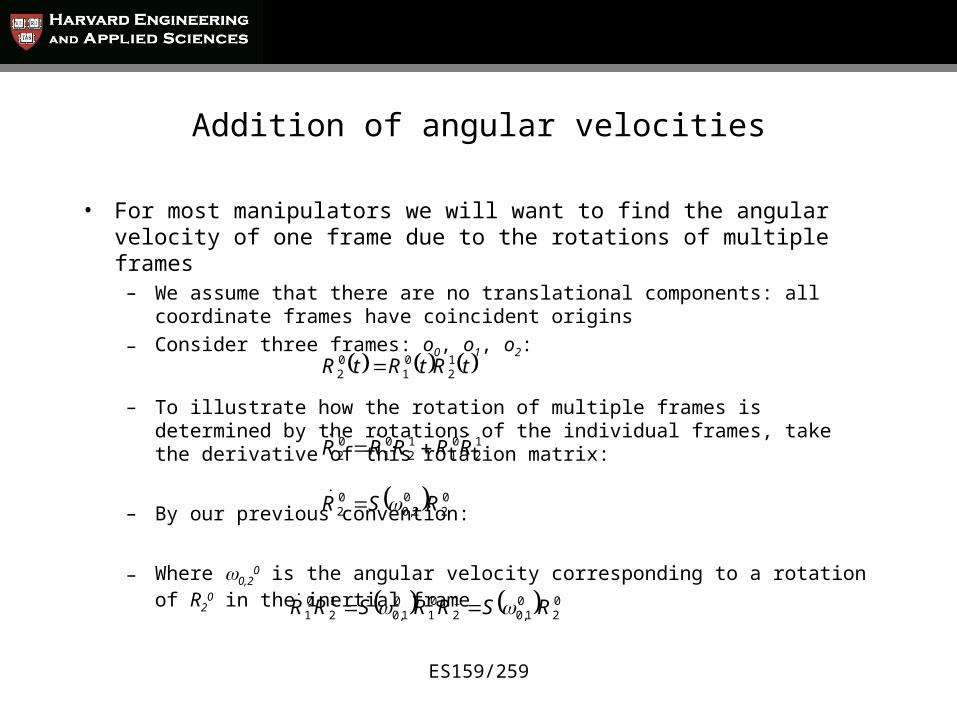
• For most manipulators we will want to find the angular velocity of one frame due to the rotations of multiple frames
– We assume that there are no translational components: all coordinate frames have coincident origins
– Consider three frames: o0, o1, o2:
– To illustrate how the rotation of multiple frames is determined by the rotations of the individual frames, take the derivative of this rotation matrix:
– By our previous convention:
– Where 0,20 is the angular velocity corresponding to a rotation of R2
0 in the inertial frame
tRtRtR 12
01
02
12
01
12
01
02 RRRRR
02
02,0
02 RSR
02
01,0
12
01
01,0
12
01 RSRRSRR
ES159/259
Addition of angular velocities
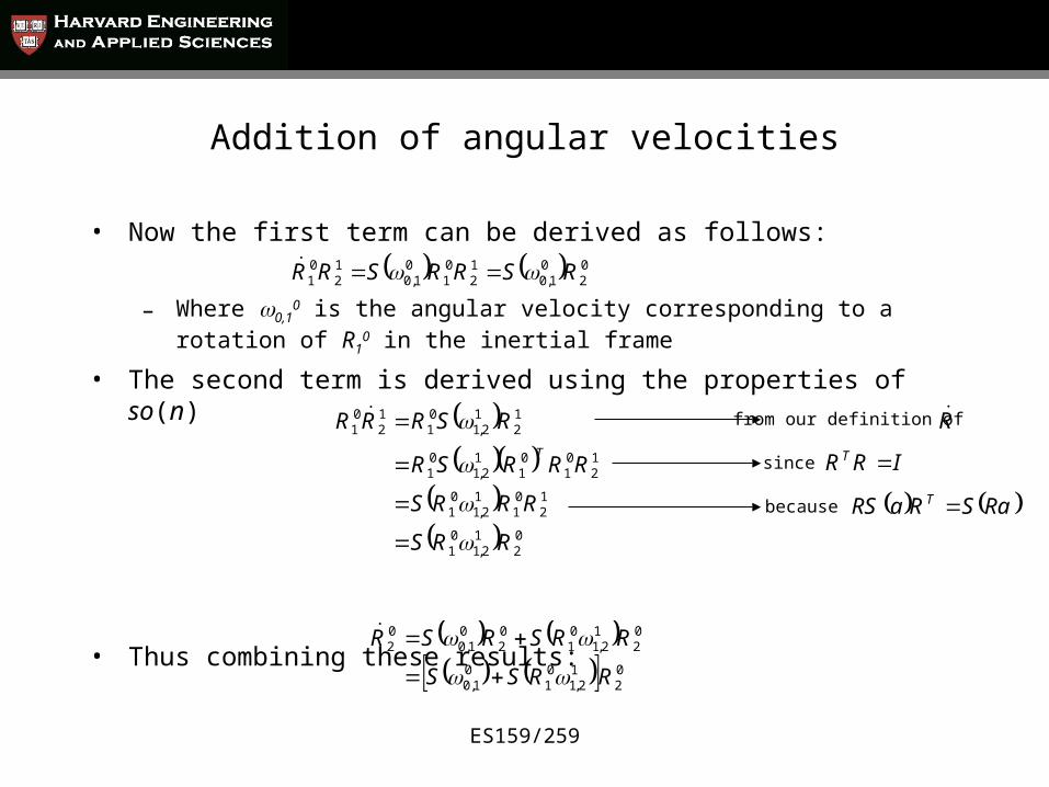
• Now the first term can be derived as follows:
– Where 0,10 is the angular velocity corresponding to a rotation of R1
0 in the inertial frame
• The second term is derived using the properties of so(n)
• Thus combining these results:
02
01,0
12
01
01,0
12
01 RSRRSRR
0
21
2,101
12
01
12,1
01
12
01
01
12,1
01
12
12,1
01
12
01
RRS
RRRS
RRRSR
RSRRRT
from our definition of R
since IRRT
RaSRaRS T because
0
21
2,101
01,0
02
12,1
01
02
01,0
02
RRSS
RRSRSR

ES159/259
Addition of angular velocities
• Further:
• And since
• Therefore angular velocities can be added once they are projected into the same coordinate frame.
• This can be extended to calculate the angular velocity for an n-link manipulator:
– Suppose we have an n-link manipulator whose coordinate frames are related as follows:
– Now we want to find the rotation of the nth frame in the inertial frame:
– We can define the angular velocity of the tool frame in the inertial frame:
02
12,1
01
01,0
02
02,0 RRSSRS
bSaSbaS 1
2,101
01,0
02,0 R
112
01
0 nnn RRRR
00,0
0nnn RSR
0,1
04,3
03,2
02,1
01,0
1,1
01
34,3
03
23,2
02
12,1
01
01,0
0,0
...
...
nn
nnnnn RRRR
ES159/259
Linear velocities
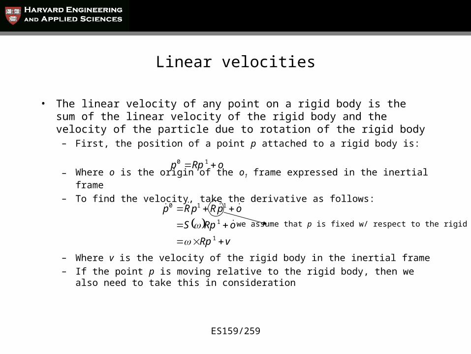
• The linear velocity of any point on a rigid body is the sum of the linear velocity of the rigid body and the velocity of the particle due to rotation of the rigid body
– First, the position of a point p attached to a rigid body is:
– Where o is the origin of the o1 frame expressed in the inertial frame
– To find the velocity, take the derivative as follows:
– Where v is the velocity of the rigid body in the inertial frame– If the point p is moving relative to the rigid body, then we also need to take
this in consideration
oRpp 10
vRp
oRpS
opRpRp
1
1
110
we assume that p is fixed w/ respect to the rigid body
ES159/259
The Jacobian
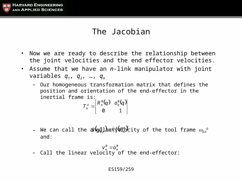
• Now we are ready to describe the relationship between the joint velocities and the end effector velocities.
• Assume that we have an n-link manipulator with joint variables q1, q2, …, qn
– Our homogeneous transformation matrix that defines the position and orientation of the end-effector in the inertial frame is:
– We can call the angular velocity of the tool frame 0,n0 and:
– Call the linear velocity of the end-effector:
Tnnn RRS 000,0
10
00 qoqRT nno
n
00nn ov
ES159/259
The Jacobian
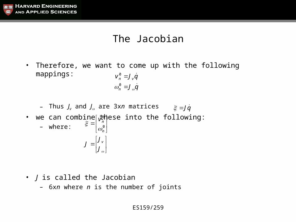
• Therefore, we want to come up with the following mappings:
– Thus Jv and J are 3xn matrices
• we can combine these into the following:– where:
• J is called the Jacobian– 6xn where n is the number of joints
qJ
qJv
n
vn
0
0
qJ
J
JJ
v
v
n
n0
0
ES159/259
Deriving J
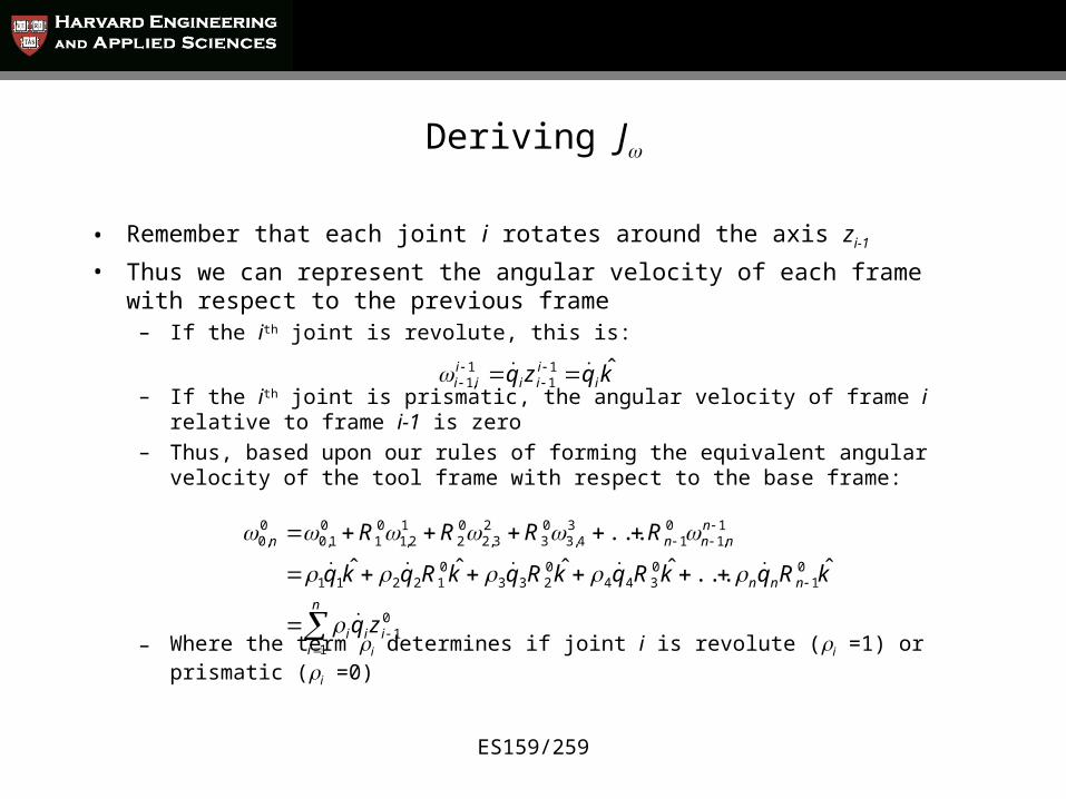
• Remember that each joint i rotates around the axis zi-1
• Thus we can represent the angular velocity of each frame with respect to the previous frame
– If the ith joint is revolute, this is:
– If the ith joint is prismatic, the angular velocity of frame i relative to frame i-1 is zero
– Thus, based upon our rules of forming the equivalent angular velocity of the tool frame with respect to the base frame:
– Where the term i determines if joint i is revolute (i =1) or prismatic (i =0)
kqzq iiii
iii
ˆ11
1,1
01
1
01
0344
0233
012211
1,1
01
34,3
03
23,2
02
12,1
01
01,0
0,0
ˆ...ˆˆˆˆ
...
i
n
iii
nnn
nnnnn
zq
kRqkRqkRqkRqkq
RRRR
ES159/259
Deriving J
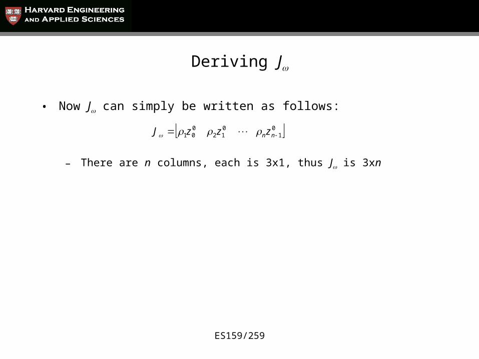
• Now J can simply be written as follows:
– There are n columns, each is 3x1, thus J is 3xn
01
012
001 nnzzzJ
ES159/259
Deriving Jv
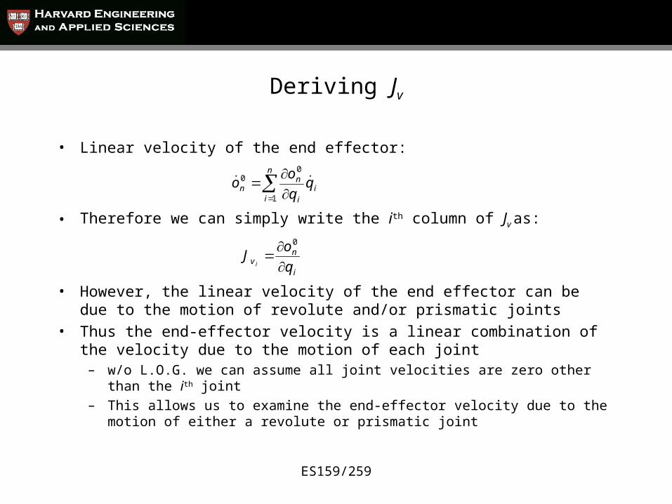
• Linear velocity of the end effector:
• Therefore we can simply write the ith column of Jv as:
• However, the linear velocity of the end effector can be due to the motion of revolute and/or prismatic joints
• Thus the end-effector velocity is a linear combination of the velocity due to the motion of each joint
– w/o L.O.G. we can assume all joint velocities are zero other than the ith joint– This allows us to examine the end-effector velocity due to the motion of
either a revolute or prismatic joint
n
ii
i
nn q
q
oo
1
00
i
nv q
oJ
i
0

ES159/259
Deriving Jv
• End-effector velocity due to prismatic joints– Assume all joints are fixed other than the prismatic joint di
– The motion of the end-effector is pure translation along zi-1
– Therefore, we can write the ith column of the Jacobian:
01
01
0
1
0
0
iiiin zdRdo
01 iv zJ
i
ES159/259
Deriving Jv
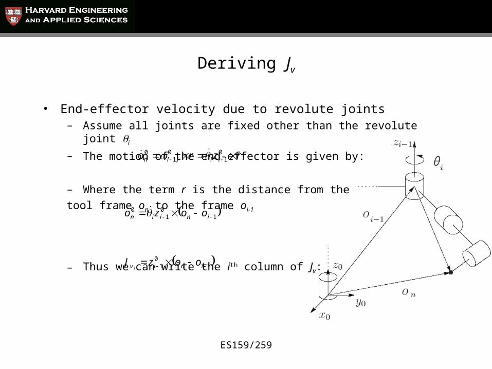
• End-effector velocity due to revolute joints– Assume all joints are fixed other than the revolute joint i
– The motion of the end-effector is given by:
– Where the term r is the distance from the
tool frame on to the frame oi-1
– Thus we can write the ith column of Jv:
rzro iiiin 0
10
,10
10
10
iniin oozo
10
1 iniv oozJi
ES159/259
The complete Jacobian
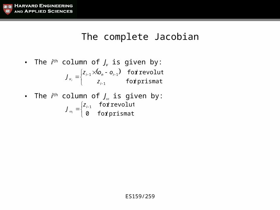
• The ith column of Jv is given by:
• The ith column of J is given by:
prismatic for
revolute for
1
11
iz
ioozJ
i
iniv i
prismatic for0
revolute for1
i
izJ i
i

ES159/259
Example: two-link planar manipulator
• Calculate J for the following manipulator:– Two joint angles, thus J is 6x2
– Where:
01
00
120102
00
zz
oozoozqJ
0
,
0
,
0
0
0
12211
12211
211
11
10 sasa
caca
osa
ca
oo
1
0
001
00 zz
11
00
00
0012212211
12212211
cacaca
sasasa
qJ
ES159/259
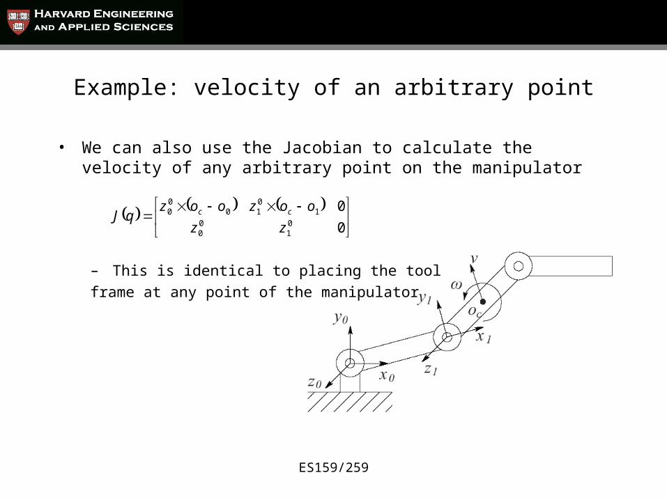
Example: velocity of an arbitrary point
• We can also use the Jacobian to calculate the velocity of any arbitrary point on the manipulator
– This is identical to placing the tool
frame at any point of the manipulator
0
001
00
1010
00
zz
oozoozqJ cc

ES159/259
Example: Stanford manipulator
• The configuration of the Stanford manipulator allows us to make the following simplifications:
• Where o is the common origin of the o3, o4, and o5 frames
6,5,4 ,
0
2,1 ,
1
61
23
1
161
iz
oozJ
zJ
iz
oozJ
i
ii
i
iii
ES159/259
Example: Stanford manipulator
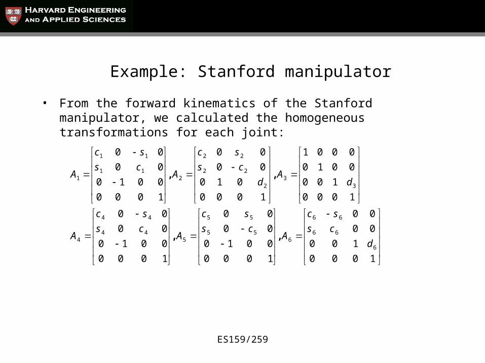
• From the forward kinematics of the Stanford manipulator, we calculated the homogeneous transformations for each joint:
1000
100
00
00
1000
0010
00
00
1000
0010
00
00
1000
100
0010
0001
1000
010
00
00
1000
0010
00
00
6
66
66
655
55
544
44
4
33
2
22
22
211
11
1
d
cs
sc
Acs
sc
Acs
sc
A
dA
d
cs
sc
Acs
sc
A
, ,
, ,
ES159/259
Example: Stanford manipulator
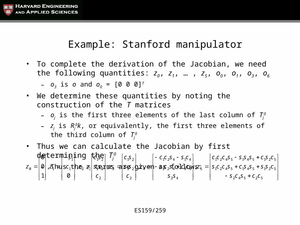
• To complete the derivation of the Jacobian, we need the following quantities: z0, z1, … , z5, o0, o1, o3, o6
– o3 is o and o0 = [0 0 0]T
• We determine these quantities by noting the construction of the T matrices
– oj is the first three elements of the last column of Tj0
– zj is Rj0k, or equivalently, the first three elements of the third column of Tj
0
• Thus we can calculate the Jacobian by first determining the Tj0
– Thus the zi terms are given as follows:
52542
5215415421
5215415421
5
42
41421
41421
4
2
21
21
3
2
21
21
21
1
10 , , , ,
0
,
1
0
0
ccscs
csssscsccs
cscssssccc
z
ss
ccscs
csscc
z
c
ss
sc
z
c
ss
sc
zc
s
zz
ES159/259
Example: Stanford manipulator
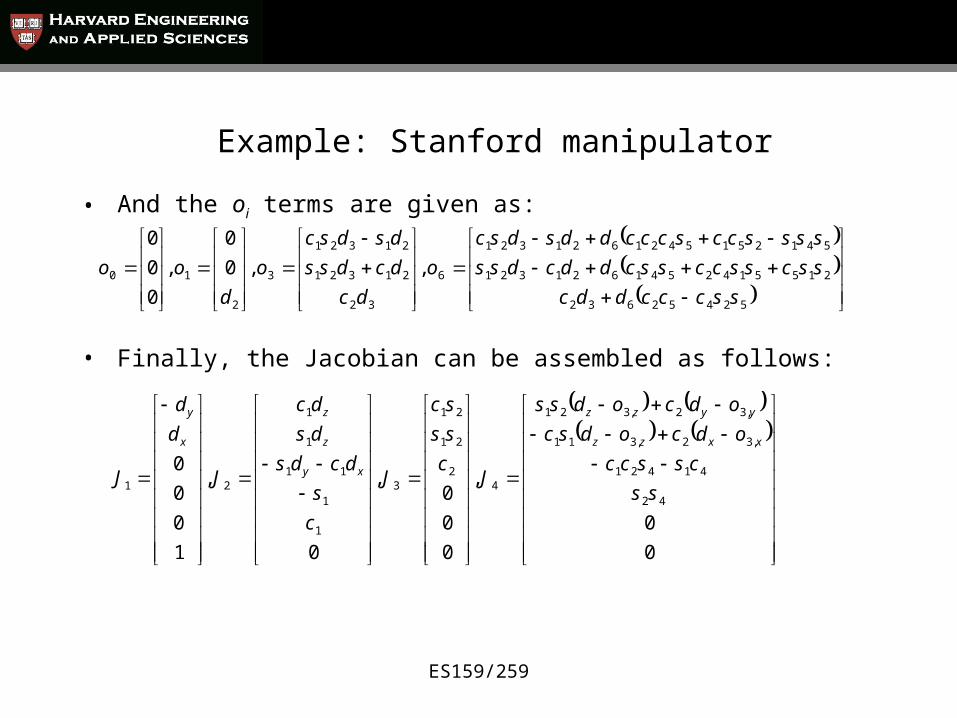
• And the oi terms are given as:
• Finally, the Jacobian can be assembled as follows:
52452632
2155142541621321
5412515421621321
6
32
21321
21321
3
2
10 , ,0
0
,
0
0
0
sscccddc
sscssccsscddcdss
ssssccscccddsdsc
o
dc
dcdss
dsdsc
o
d
oo
0
0
,
0
0
0 ,
0
,
1
0
0
0
42
41421
,32,311
,32,321
42
21
21
3
1
1
11
1
1
21 ss
csscc
odcodsc
odcodss
Jc
ss
sc
J
c
s
dcds
ds
dc
J
d
d
J
xxzz
yyzz
xy
z
z
x
y
ES159/259
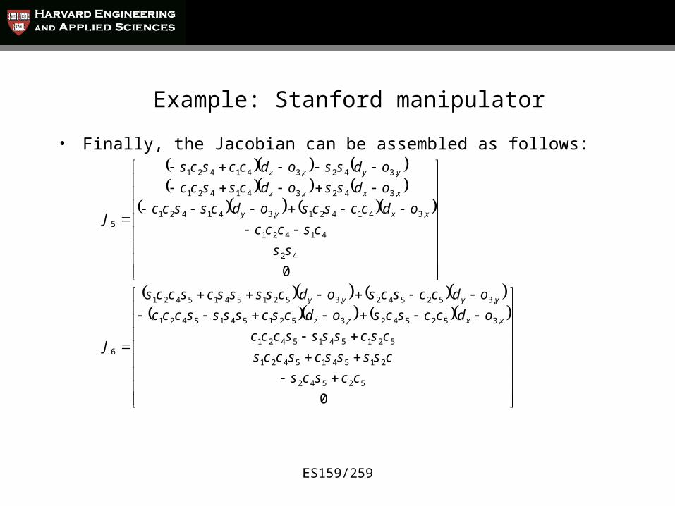
Example: Stanford manipulator
• Finally, the Jacobian can be assembled as follows:
0
0
52542
215415421
5215415421
,352542,35215415421
,352542,35215415421
6
42
41421
,341421,341421
,342,341421
,342,341421
5
ccscs
csssscsccs
cscssssccc
odccscsodcscssssccc
odccscsodcsssscsccs
J
ss
csccc
odccscsodcsscc
odssodcsscc
odssodccscs
J
xxzz
yyyy
xxyy
xxzz
yyzz
ES159/259
Example: SCARA manipulator
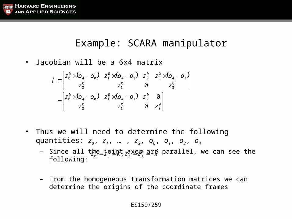
• Jacobian will be a 6x4 matrix
• Thus we will need to determine the following quantities: z0, z1, … , z3, o0, o1, o2, o4
– Since all the joint axes are parallel, we can see the following:
– From the homogeneous transformation matrices we can determine the origins of the coordinate frames
03
01
00
0214
0104
00
03
01
00
3403
0214
0104
00
0
0
0
zzz
zoozooz
zzz
oozzoozoozJ
kzzkzz ˆ ,ˆ 03
02
01
00
ES159/259
Example: SCARA manipulator
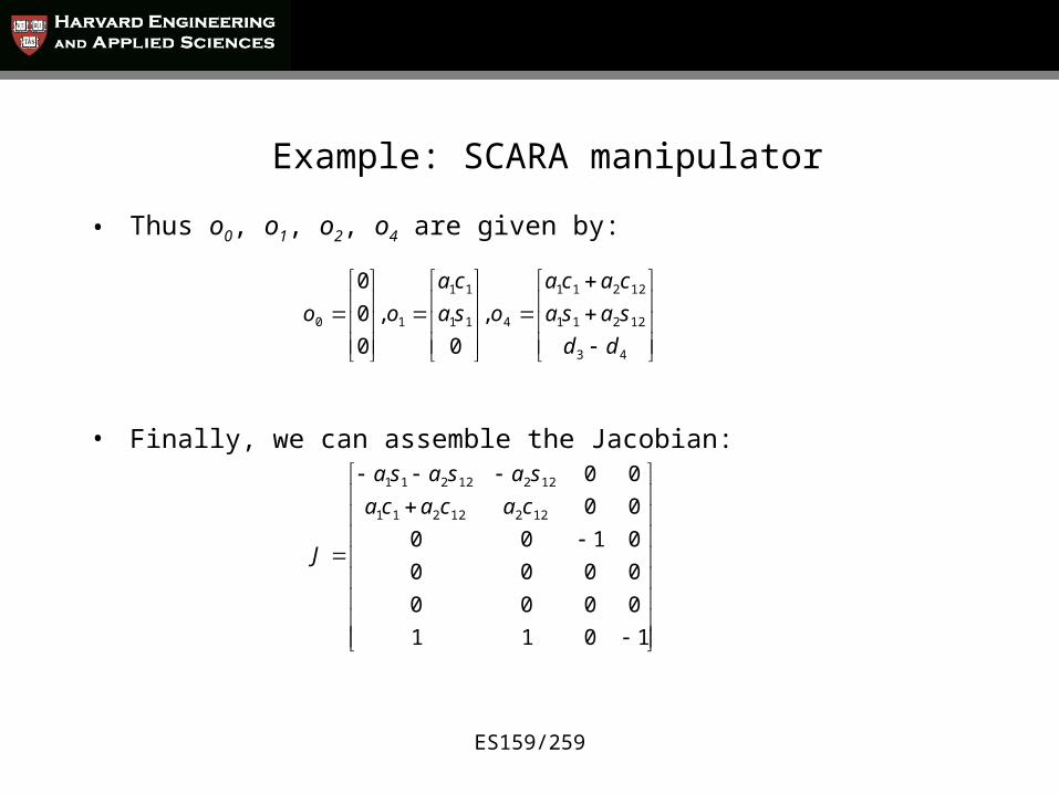
• Thus o0, o1, o2, o4 are given by:
• Finally, we can assemble the Jacobian:
43
12211
12211
411
11
10 ,
0
,
0
0
0
dd
sasa
caca
osa
ca
oo
1011
0000
0000
0100
00
00
12212211
12212211
cacaca
sasasa
J
ES159/259
Next class…
• Formal definition of singularities
• Tool velocity
• manipulability