eserve ank of eview november ecember · federalrreserve bank of st. louis eview november/december...

FEDERAL RESERVE BANK OF ST. LOUIS

R E V IE WVOLUME 86, NUMBER 6NOVEMBER/DECEMBER 2004

The Increasing Importance of Proximity for Exports from U.S. States

Cletus C. Coughlin

Monetary Policy and Asset Prices: A Look Back at PastU.S. Stock Market Booms

Michael D. Bordo and David C. Wheelock

What Does the Federal Reserve’s Economic Value ModelTell Us About Interest Rate Risk at U.S. Community Banks?

Gregory E. Sierra and Timothy J. Yeager

Discrete Policy Changes and Empirical Modelsof the Federal Funds Rate

Michael J. Dueker and Robert H. Rasche

FED

ER

AL

RESER

VE

BA

NK

OF

ST

LO

UIS

RE

VIE

WN

OV

EM

BE

R/D

EC

EM

BE

R2004 • V

OLU

ME

86,N

UM

BE

R6

NOVEMBER/DECEMBER 2004 i

ContentsVolume 86, Number 6

1 The Increasing Importance of Proximityfor Exports from U.S. States

Cletus C. Coughlin

Changes in income, trade policies, transporta-tion costs, technology, and many other variablesaffect the geographic pattern of internationaltrade flows. This paper focuses on the changinggeography of merchandise exports from indi-vidual U.S. states to foreign countries. Generallyspeaking, the geographic distribution of stateexports has changed so that trade has becomemore intense with nearby countries relative todistant countries. All states, however, did notexperience similar changes. As measured bythe distance of trade, which is the averagedistance that a state’s international trade istransported, 40 states experienced a decliningdistance of trade, while 11 states (includingWashington, D.C.) experienced an increasingdistance of trade. Evidence, albeit far fromdefinitive, suggests that declining transportationcosts over land, the implementation of theNorth American Free Trade Agreement, andfaster income growth by nearby trading partnersrelative to distant partners have contributedto the changing geography of state exports.

19 Monetary Policy and Asset Prices: A LookBack at Past U.S. Stock Market Booms

Michael D. Bordo and David C. Wheelock

This article examines the economic environ-ments in which past U.S. stock market boomsoccurred as a first step toward understandinghow asset price booms come about andwhether monetary policy should be used todefuse booms. The authors identify severalepisodes of sustained rapid rises in equityprices in the 19th and 20th centuries, and thenassess the growth of real output, productivity,the price level, and money and credit stocksduring each episode. Two booms stand out interms of their length and rate of increase inmarket prices—the booms of 1923-29 and1994-2000. In general, the authors find thatbooms occurred in periods of rapid real growth

Director of Research

Robert H. Rasche

Deputy Director of Research

Cletus C. Coughlin

Review Editor

William T. Gavin

Research Economists

Richard G. Anderson

James B. Bullard

Riccardo DiCecio

Michael J. Dueker

Thomas A. Garrett

Hui Guo

Rubén Hernández-Murillo

Kevin L. Kliesen

Christopher J. Neely

Edward Nelson

Michael T. Owyang

Michael R. Pakko

Anthony N.M. Pennington-Cross

Jeremy M. Piger

Patricia S. Pollard

Daniel L. Thornton

Howard J. Wall

Christopher H. Wheeler

David C. Wheelock

Managing Editor

George E. Fortier

Assistant Editor

Lydia H. Johnson

Graphic Designer

Donna M. Stiller

Review is published six times per year by the Research Division of theFederal Reserve Bank of St. Louis and may be accessed at our webaddress: research.stlouisfed.org/publications/review. Single-copy subscriptions are also available free of charge. Send requeststo: Federal Reserve Bank of St. Louis, Public Affairs Department, P.O.Box 442, St. Louis, MO 63166-0442, or call (314) 444-8808 or 8809.

The views expressed are those of the individual authors and do notnecessarily reflect official positions of the Federal Reserve Bank of St. Louis, the Federal Reserve System, or the Board of Governors.

© 2004, The Federal Reserve Bank of St. Louis.

Articles may be reprinted, reproduced, published, distributed, displayed,and transmitted in their entirety if this copyright notice is included.Please send a copy of any reprinted, published, or displayed materialsto George Fortier, Research Division, Federal Reserve Bank of St. Louis,P.O. Box 442, St. Louis, MO 63166-0442; [email protected] note: Abstracts, synopses, and other derivative works may bemade only with prior written permission of the Federal Reserve Bank of St. Louis. Please contact the Research Division at the above address to request permission.

ISSN 0014-9187

R E V I E W

and productivity advancement, suggesting thatbooms are driven at least partly by funda-mentals. They find no consistent relationshipbetween inflation and stock market booms,though booms have typically occurred whenmoney and credit growth were above average.

45 What Does the Federal Reserve’s EconomicValue Model Tell Us About Interest RateRisk at U.S. Community Banks?

Gregory E. Sierra and Timothy J. Yeager

The savings and loan crisis of the 1980srevealed the vulnerability of some depositoryinstitutions to changes in interest rates. Sincethat episode, U.S. bank supervisors have placedmore emphasis on monitoring the interest raterisk of commercial banks. Economists at theBoard of Governors of the Federal ReserveSystem developed a duration-based economicvalue model (EVM) designed to estimate theinterest rate sensitivity of banks. The authorstest whether measures derived from the Fed’sEVM are correlated with the interest rate sensi-tivity of U.S. community banks. The answer tothis question is important because bank super-visors rely on EVM measures for monitoringand risk-scoping bank-level interest rate sensi-tivity. The authors find that the Federal Reserve’sEVM is indeed correlated with banks’ interestrate sensitivity and conclude that supervisorscan rely on this tool to help assess a bank’sinterest rate risk. These results are consistentwith prior research that finds the average inter-est rate risk at banks to be modest, though thepotential interaction between interest rate riskand other risk factors is not considered here.

61 Discrete Policy Changes and EmpiricalModels of the Federal Funds Rate

Michael J. Dueker and Robert H. Rasche

Empirical models of the federal funds ratealmost uniformly use the quarterly or monthlyaverage of the daily rates. One empirical ques-tion about the federal funds rate concerns theextent to which monetary policymakers smooththis interest rate. Under the hypothesis of ratesmoothing, policymakers set the interest ratethis period equal to a weighted average of therate inherited from the previous quarter and therate implied by current economic conditions,such as the Taylor rule rate. Perhaps surpris-ingly, however, little attention has been givento measuring the interest rate inherited fromthe previous quarter. Previous tests for interestrate smoothing have assumed that the quarterlyor monthly average from the previous periodis the inherited rate. The authors of this study,in contrast, suggest that the end-of-quarter levelof the target federal funds rate is the inheritedrate, and empirical tests support this proposi-tion. The authors show that this alternativeview of the rate inherited from the past affectsempirical results concerning interest ratesmoothing, even in relatively rich models thatinclude regime switching.

73 Review Index 2004

ii NOVEMBER/DECEMBER 2004

R E V I E W

over time, then its trade is becoming more (less)intense with nearer countries relative to countriesfarther away. In other words, a declining (increasing)distance of trade means that the shares of a country’s(state’s) trade with nearby trading partners is rising(falling) relative to trade with its more distant tradingpartners.

The analysis begins by summarizing the factsand the explanations concerning the geographicdistribution of exports throughout the world. Animportant feature of the economic geography oftrade flows is the distance that separates a state fromits trading partners. Distance is generally thoughtto play a key role in the geographic distribution oftrade for two reasons. First, transportation costs arehigher for longer distances. Second, the costs ofaccessing information about foreign markets andestablishing a trade relationship in those marketsare higher for longer distances.2 Thus, a country’strade with more distant countries is deterred.

Despite the “death of distance” associated withthe communications revolution, proximity appearsto be increasingly important for trade flows.3 Usingthe bilateral trade flows of 150 countries, Carrereand Schiff (2004) find that during 1962-2000 thedistance of (non-fuel merchandise) trade declinesfor the average country and that countries with adeclining distance of trade were twice as numer-ous as those with an increasing distance of trade.

After reviewing the geography of exports fromthe perspective of individual countries throughoutthe world, I examine the geography of the exports

2 See Rauch (1999) for additional discussion of this point.

3 The death of distance has become a popular term because of TheDeath of Distance: How the Communications Revolution Will ChangeOur Lives by Frances Cairncross (1997). The book focuses on theeconomic and social importance of how advances in technology havevirtually eliminated distance as a cost in communicating ideas anddata. Possibly, this death of distance has made foreign direct investmentand trade with proximate countries a more efficient way to servemarkets than trade over long distances.

The Increasing Importance of Proximity for Exports from U.S. StatesCletus C. Coughlin

I ncome, trade policies, transportation costs,technology, and many other variables combineto determine the levels of international trade

flows. Not only do changes in these determinantsaffect the levels of trade flows, they can also haveimportant consequences for the geographic patternof a country’s trade. Some changes are generallythought to increase the proportion of a country’strade with nearby countries relative to its othertrading partners, while other changes tend todecrease this proportion. For example, if a countryenters into a trade agreement with nearby countries,it is likely that the country’s share of trade withnearby countries will increase relative to its tradewith other trading partners. On the other hand,declining transportation costs can reduce the costdisadvantage of trading with distant countries andcould thereby increase trade with more distantcountries relative to those nearby.

This paper focuses on the changing geographyof merchandise exports from individual U.S. statesto foreign countries. Due to data limitations, exportsof services are not examined. Two basic questions areaddressed. First, how has the geographic distribu-tion of exports from individual U.S. states changed?Second, which changes in the economic environ-ment appear to account for the observed changesin the geographic distribution of state exports?

A useful measure for analyzing the changinggeography of trade is the distance of trade, which issimply the average distance that a country’s (state’s)international trade is transported.1 If a country’s(state’s) distance of trade is declining (increasing)

NOVEMBER/DECEMBER 2004 1

1 The calculation is straightforward. Assume a state’s exports areshipped to two countries and that the value of exports sent to onecountry, which is 1,000 miles away, is $800 and the value sent to theother country, which is 3,000 miles away, is $1,200. Thus, 40 percentof the state’s exports are transported 1,000 miles and 60 percent aretransported 3,000 miles. The distance of trade is 2,200 miles (40% ×1,000+60% × 3,000).

Cletus C. Coughlin is deputy director of research at the Federal Reserve Bank of St. Louis. Molly D. Castelazo provided research assistance.

Federal Reserve Bank of St. Louis Review, November/December 2004, 86(6), pp. 1-18.© 2004, The Federal Reserve Bank of St. Louis.

Coughlin R E V I E W

2 NOVEMBER/DECEMBER 2004

from individual U.S. states to their trading-partnercountries. The distance of trade is calculated annu-ally for each state beginning in 1988, the first yearof detailed geographic data for individual states.Similar to the finding for the majority of countries,the majority of, but not all, states show a decliningdistance of trade.

The findings for individual states allow for anexamination of some explanations that may accountfor the changing geographic distribution of exportsat the state level. The uneven income growth oftrading partners, the implementation of the NorthAmerican Free Trade Agreement (NAFTA), and chang-ing transportation costs are the “usual suspects.”Possibly, incomes of nearby trading partners haveincreased more rapidly than incomes of more dis-tant trading partners. Such a development mightstimulate trade with nearby trading partners (rela-tive to those more distant) so that a state’s distanceof trade declines. Similarly, the implementation ofNAFTA, by reducing trade barriers between theUnited States and its major North American tradingpartners, might tend to decrease a state’s distanceof trade. Finally, it is possible that transportationcosts have changed to increase the attractivenessof trading with nearby countries. My goal is to pro-vide suggestive evidence on how these three factorshave changed the geography of the exports of states,which in turn provides insights concerning thechanging geography of total U.S. exports.

THE CHANGING GEOGRAPHY OFWORLD TRADE

During the second half of the twentieth century,the volume of international trade throughout theworld increased more rapidly than output. Baier andBergstrand (2001) attempted to identify the reasonsfor the growth of international trade between thelate 1950s and the late 1980s. They estimated thatdeclines in transportation costs explained about 8percent of the average trade growth of severaldeveloped countries, tariff-rate reductions about25 percent, and income growth the remaining 67percent. The question for the current study isstraightforward. Have these determinants, whichare related to one another, changed in such a waythat would alter systematically the geography ofstate export flows? To date, systematic evidencerelating these determinants to state export flows islacking. In fact, little evidence exists as to howchanges in these determinants of trade have affectedthe geography of world trade flows.

Changing Transportation Costs—Usual Suspect No. 1

The costs of transporting goods from a producerin one country to a final user in another country arelarge. Putting a precise number on “large” is verydifficult and undoubtedly varies across goods andcountries. Despite this difficulty, Anderson andvan Wincoop (forthcoming) estimate internationaltransportation costs for industrialized countries tobe equivalent to a tax of 21 percent. Additional trans-portation costs are incurred to move internationallytraded goods within exporting countries and withinimporting countries. Not surprisingly, changes intransportation costs can have large effects on tradeflows. Not only can reductions in transportationcosts lead to increased trade flows directly, but alsoindirectly by affecting the profitability of productionin specific locations.

A point that might not be intuitively obvious isthat a decline in transportation costs might causeeither an increase or a decrease in a country’s (state’s)distance of trade. In the context of ocean shippingcosts, it depends on the nature of the change intransportation costs.

Ocean shipping transportation costs can bedivided into those unrelated to distance, known asdwell costs, and those related to distance, known asdistance costs. Dwell costs cover various aspects,such as the cost of loading and unloading ships andthe cost (including time) of queuing outside a portwaiting to be serviced. On the other hand, distancecosts are related positively to the distance fromport to port. For example, the longer the distancebetween ports, the larger the fuel costs of transport-ing a given shipment.

In theory, reductions in both dwell costs anddistance costs increase international trade flows;however, their effects on the distance of trade differ.A reduction in dwell costs increases the incentive totrade with nearby locations relative to distant loca-tions; this is so because dwell costs make up a largerproportion of total transport costs for shorter dis-tances.4 Thus, a reduction in dwell costs tends to

4 For example, assume dwell costs of $100,000 and distance costs permile of $200. If so, then the cost of a trip of 1,000 miles is $300,000and a trip of 4,500 miles is $1 million. Thus, for the shorter (longer)trip the respective shares of the transportation costs are 33 (10) percentfor the dwell costs and 67 (90) percent for the distance costs. As aresult, a reduction in dwell costs, say from $100,000 to $50,000, hasa larger proportional effect on costs for the shorter trip; a reduction indistance costs, say from $200 per mile to $100 per mile, has a largerproportional effect on costs for the longer trip.

FEDERAL RESERVE BANK OF ST. LOUIS Coughlin


reduce the distance of trade. On the other hand, areduction in distance costs increases the incentiveto trade with distant locations relative to nearbylocations. The reduced cost per mile causes a largerproportional decrease in transport costs for longerdistances. Thus, a reduction in distance costs tendsto increase the distance of trade.5

Because evidence on dwell and distance costsis limited, it is very difficult to reach firm conclusionsconcerning their evolution and, in turn, their effectson the distance of trade. Hummels (1999) providessome evidence suggesting technological changesassociated with containerization have reduced bothdwell and distance costs.6 Containerization is asystem of inter-modal transport that uses standard-sized containers that can be loaded directly ontocontainer ships, freight trains, and trucks. Dwellcosts are reduced because ships spend less time inport and the cargo can be handled more efficiently.Meanwhile, the larger and faster ships allowed bycontainerization have reduced shipping costs on aton-mile basis while the ship is moving betweenports. It is likely, however, that containerizationlowered dwell costs relatively more than distancecosts. In addition, containerization, by eliminatingthe unpacking and packing of cargoes at everychange in transport mode, likely reduced the costof the inland movement of goods by making theinter-modal transfer of goods easier. Such changesshould tend to reduce the distance of trade.

Containerization, however, is only one of themany changes that have affected transportationcosts. Regulatory policies and energy prices are twoadditional factors. Whether transportation costshave in fact declined in recent decades is uncertainbecause of the lack of evidence on this issue. Forexample, Carrere and Schiff (2004) conclude thattransportation costs have not necessarily declinedacross all modes of transportation. First, they citeevidence provided by Hummels (1999), who found

that ocean freight rates have increased, while airfreight rates have declined rapidly. Hummels alsofound evidence that overland transport costs in theUnited States have declined relative to ocean freightrates. In fact, according to Glaeser and Kohlhase(2004), the costs of moving goods by rail and bytruck within the United States have fallen substan-tially in a nearly continuous manner since 1890.7

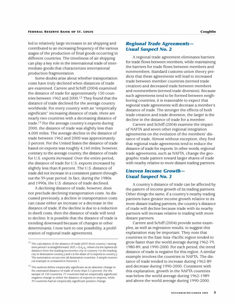
While far from precise in terms of quantifyingthe changes in transportation costs, these findingsare consistent with recent changes in the relativeshares of the methods used to transport U.S. exports.Over time, air and land shipments have displacedocean shipments. Figure 1 shows that between 1980and 2002 the shares of air and land shipmentsincreased by 11.9 and 14.5 percentage points, respec-tively, while the share of ocean shipments declinedby 26.4 percentage points. As a result, the majorityof U.S. exports are no longer shipped on oceanvessels. In fact, in 2002, shipments by air and landaccounted for larger shares of exports than ship-ments by sea.

A second source of evidence relevant to changesin transportation costs relies on studies that estimatethe relationship between distance and internationaltrade flows.8 Numerous studies have generated esti-mates of the distance sensitivity of trade or, usingmore precise terminology, the distance elasticity oftrade: that is, the percentage change in trade flowsassociated with a given percentage increase in thedistance separating one country from its tradingpartners. These studies find, not surprisingly, thatthe larger the distance that separates two countries,the smaller the value of trade moving between them.More important for the current discussion is thecommon finding that distance is playing a changingrole over time in the geographic distribution of trade.For example, results by Frankel (1997) indicate that

5 A decline in transportation costs might not affect the distance oftrade. Eichengreen and Irwin (1998) note that the cost of transportinggoods over various distances could decline proportionately. In thiscase, which they call “distance-neutral” technological progress, sucha decline in transportation costs would tend to leave the distance oftrade unchanged.

6 Hummels (1999) identified as important the following institutionalchanges that have affected ocean shipping: open registry shipping,which allows ships to be registered under flags of convenience toavoid some regulatory and manning costs imposed by some countries,and cargo reservation policies, which were to designed to ensure thata country’s own ships were granted a substantial share of that country’sliner traffic.

7 Glaeser and Kohlhase (2004) find that the cost of moving goods hasdeclined by roughly 90 percent since 1890. The costs of transportinggoods by rail and by truck have declined at annual rates of 2.5 percentand 2.0 percent, respectively. As a result, they conclude that the costof moving goods within the United States is no longer an importantcomponent of the production process.

8 Using distance as a proxy for transportation costs is problematic fornumerous reasons. Distance is generally measured with the “greatcircle” formula. Actual transportation routes are not this direct. Inaddition, the use of distance assumes one route between tradingregions. Trade between two geographically large countries, such asthe United States and Canada, is conducted over many routes. Multipleroutes and multiple modes of transportation increase the doubts thatdistance is a good proxy for transportation costs. As discussed in thetext, many transportation costs, such as dwell costs, clearly do notvary with distance. Finally, actual freight rates often bear little connec-tion to distance traveled.



if the distance separating a country from two of itstrading partners differed by 10 percent, then tradeflows between the country and its more distant trad-ing partner (relative to the country and its nearbypartner) were 4 percent less during the 1960s and7 percent less during the 1990s. Overall, the majorityof studies indicate that the distance sensitivity oftrade is not shrinking, but rather increasing.9 Such

a change would tend to decrease the distance oftrade.

A third piece of evidence concerning transporta-tion costs highlights the impact of time.10 The costconsequences of delays can be quite large. Hummels(2001) has estimated that each day saved in shippingtime was worth 0.8 percent of the value of manu-factured goods. Overall, faster transport between1958 and 1998 due to increased air shipping andspeedier ocean vessels was equivalent to reducingtariffs on manufactured goods from 32 percent to 9percent.11

Time costs have likely played a key role in thechange in shipping modes. Because shipping by airis much faster than shipping by sea, the decline inair shipping prices relative to ocean shipping priceshas made the saving of time less expensive. This has

11 In general, transportation costs, including time costs, have risen as aresult of the terrorist attacks of September 11, 2001. Insurance rates,especially for shipping in the Middle East, have increased sharply.Additional scrutiny of containers has also increased costs. Accordingto the Organisation for Economic Co-operation and Development(2002), these costs could run from 1 to 3 percent of trade. Moreover,additional security measures cause delays for importers and exportersthat further increase transportation costs.

U.S. Exports by Transport Mode, 1980-2002

60

50

40

30

20

10

01980 1982 1984 1986 1988 1990 1992 1994 1996 1998 2000 2002

NOTE: The variable Land was created by subtracting the sum of air and vessel exports fromtotal exports.SOURCE: U.S. Bureau of the Census.

Sea

Land

Air

Figure 1

9 Disdier and Head (2004), in a thorough examination of numerousstudies using gravity models, conclude that the impact of distance isincreasing, albeit slightly, over time. Brun et al. (2003) and Coe et al.(2002) reach a similar conclusion. Berthelon and Freund (2004) findthat, rather than a shift in the composition of trade, an increase inthe distance sensitivity for more than 25 percent of the industriesexamined accounts for this result. Research by Rauch (1999), contraryto most studies, finds that the effect of increased distance on tradehas declined since 1970.

10 Hummels (2001) identified numerous costs associated with shippingtime and its variability. Lengthy and variable shipping times cause firmsto incur inventory and depreciation costs. Inventory-holding costsinclude the financing costs of goods in transit and the costs of main-taining larger inventories at final destinations to handle variation inarrival times. Examples of depreciation, which reflect any reason toprefer a newer good to an older good, include the spoilage of goods(fresh produce), goods with timely information content (newspapers),and goods with characteristics whose demand is difficult to forecast(fashion apparel).



led to relatively large increases in air shipping andcontributed to an increasing frequency of the variousstages of the production of final goods occurring indifferent countries. The timeliness of air shippingcan play a key role in the international trade of inter-mediate goods that characterizes internationalproduction fragmentation.

Some doubts arise about whether transportationcosts have truly declined when distances of tradeare examined. Carrere and Schiff (2004) examinedthe distance of trade for approximately 150 coun-tries between 1962 and 2000.12 They found that thedistance of trade declined for the average countryworldwide. For every country with an “empiricallysignificant” increasing distance of trade, there arenearly two countries with a decreasing distance oftrade.13 For the average country’s exports during2000, the distance of trade was slightly less than4,000 miles. The average decline in the distance oftrade between 1962 and 2000 was approximately5 percent. For the United States the distance of tradebased on exports was roughly 4,160 miles; however,contrary to the average country, the distance of tradefor U.S. exports increased. Over the entire period,the distance of trade for U.S. exports increased byslightly less than 8 percent. The U.S. distance oftrade did not increase in a consistent pattern through-out the 39-year period. In fact, during the 1980sand 1990s, the U.S. distance of trade declined.

A declining distance of trade, however, doesnot preclude declining transportation costs. As dis-cussed previously, a decline in transportation costscan cause either an increase or a decrease in thedistance of trade. If the decline is due to a reductionin dwell costs, then the distance of trade will tendto decline. It is possible that the distance of trade istrending downward because of changes in otherdeterminants. I now turn to one possibility, a prolif-eration of regional trade agreements.

Regional Trade Agreements—Usual Suspect No. 2

A regional trade agreement eliminates barriersfor trade flows between members, while maintainingthe barriers for trade flows between members andnonmembers. Standard customs union theory pre-dicts that these agreements will lead to increasedtrade between member countries (termed tradecreation) and decreased trade between membersand nonmembers (termed trade diversion). Becausesuch agreements tend to be formed between neigh-boring countries, it is reasonable to expect thatregional trade agreements will decrease a member’sdistance of trade. The stronger the effects of bothtrade creation and trade diversion, the larger is thedecline in the distance of trade for a member.

Carrere and Schiff (2004) examine the impactof NAFTA and seven other regional integrationagreements on the evolution of the members’ dis-tance of trade. Almost without exception, they findthat regional trade agreements tend to reduce thedistance of trade for exports. In other words, regionaltrade agreements, such as NAFTA, change the geo-graphic trade pattern toward larger shares of tradewith nearby relative to more distant trading partners.

Uneven Income Growth—Usual Suspect No. 3

A country’s distance of trade can be affected bythe pattern of income growth of its trading partners.Other things the same, if a country’s nearby tradingpartners have greater income growth relative to itsmore distant trading partners, the country’s distanceof trade will decline because trade with its nearbypartners will increase relative to trading with moredistant partners.

Carrere and Schiff (2004) provide some exam-ples, as well as regression results, to suggest thisexplanation may be important. They note thatcountries in the East Asia–Pacific region tended togrow faster than the world average during 1962-79,1980-89, and 1990-2000. For each period, the trenddistance of trade is negative for this region. A similarexample involves the countries in NAFTA. The dis-tance of trade tended to increase during 1962-89and decrease during 1990-2000. Consistent withthis explanation, growth in the NAFTA countrieswas below the world average during 1962-1989and above the world average during 1990-2000.

12 The calculation of the distance of trade (DOT) from country i duringtime period t is straightforward. DOTi=Σ dij sij, where d is the (spherical)distance from the leading (economic) city in country i to the leadingcity in destination country j and s is the share of i’s exports to country j.The summation occurs over all destination countries. A simple numeri-cal example is contained in footnote 1.

13 The authors define empirically significant as an absolute change inthe estimated distance of trade of more than 5.5 percent. For thesample of 150 countries, 77 countries had an empirically significantnegative change in either the distance of exports or imports, while39 countries had an empirically significant positive change.



International Production Fragmentation—A New Suspect

In addition to the usual suspects, one new sus-pect has emerged: international production fragmen-tation. This development has led to major changesin the location of production and trade flows. A lackof data precludes an empirical examination of thisexplanation for state-level exports. Nonetheless, forcompleteness, a brief discussion of the relationshipbetween international production fragmentationand the distance of trade seems warranted.

One feature of the expanding integration ofworld markets is that companies are outsourcingincreasing amounts of the production process. Thisinternationalization of production allows firms toachieve productivity gains by taking advantage ofproximity to markets and/or low-cost labor. The neteffect on the distance of trade is unclear. Despitelocating production close to markets, the likely reduc-tion in the distance of trade is uncertain because itis unclear how the increased use of low-cost laborwill affect the distance of trade. One can easily findexamples for the United States, such as the growthof maquiladoras in Mexico, which are associatedwith a declining distance of trade. On the other hand,the increased use by U.S. firms of low-cost labor inChina tends to increase the distance of trade.

Another factor contributing to a declining dis-tance of trade for the United States is the increasinguse of “just-in-time” inventory management. Newinformation and communications technology havepropelled this management. For industries, suchas apparel, in which timely delivery has becomeincreasingly important, the distance of trade hasdecreased. Evans and Harrigan (2003) show that U.S.

apparel imports have shifted from Asian countriesto Mexico and Caribbean countries.14

The increasing importance of internationalproduction fragmentation is consistent with findingsby Berthelon and Freund (2004) on the increasingdistance sensitivity of trade. They find an increasingdistance sensitivity of trade for 25 percent of theindustries they examined. Accordingly, trade withnearby countries has become more attractive relativeto trade with more distant countries. This increasingdistance sensitivity might be the result of techno-logical change that enhances the advantages ofproximity. One consequence of this change is anincreased share of trade between the countrieswithin a region, such as between the countries inNorth and South America, relative to trade acrossregions, such as between countries in North Americaand East Asia.

GEOGRAPHY OF U.S. STATE EXPORTS

The distance of trade for the United States canbe analyzed by taking a close look at the geographyof exports using state data. In view of the decliningU.S. distance of trade during the past two decades, itis reasonable to expect that the change in the dis-tance of trade (using state export data summed overall states) will indicate relatively more intense tradewith proximate regions than with distant regions.

The data in Table 1 show how the destinationof U.S. exports has changed for three five-yearperiods during 1988-2002.15 The destinations forU.S. exports are split into Canada and Mexico, thetwo major North American trading partners of theUnited States as a whole, and then the rest of theworld is split roughly into continents. Comparing1988-92 with 1998-2002, it is clear that Canada,Mexico, and Latin America and the Caribbean arethe destinations for increasing shares of U.S. exports,while Europe, Asia, Africa, and Oceania are thedestinations for decreasing shares of U.S. exports.The shift in the share between the regions with an

14 Abernathy et al. (1999) argue that three retail apparel/textile regionsare developing in the world—the United States plus Mexico and theCaribbean Basin, Japan plus East and Southeast Asia, and WesternEurope plus Eastern Europe and North Africa.

15 Export shares are calculated by dividing U.S. exports to each region(averaged across five-year periods) by total U.S. exports to all sevenregions (averaged across five-year periods). Regions are constructedusing the top 50 export markets for each state, which account for morethan 90 percent of each state’s total exports. The definition of regionsused for Tables 1 and 6 is not identical to the one used by Coughlinand Wall (2003).

Export Destination Share by Region (%)

1988-92 1993-97 1998-2002

Canada 20.4 22.4 23.4

Mexico 7.9 9.6 13.7

Latin America 6.4 7.8 7.4and the Caribbean

Europe 27.8 22.8 23.2

Asia 33.2 33.9 29.1

Africa 1.7 1.4 1.2

Oceania 2.5 2.2 2.0

Table 1



increasing share and those with a decreasing sharewas 9.8 percentage points. Most noteworthy werethe increases by Mexico and Canada of 5.8 and 2.9percentage points, respectively, and the decreasesin export shares for Europe and Asia of 4.6 and 4.1percentage points, respectively.

The changing export shares of proximate anddistant regions are suggestive of the changing dis-tance of trade for the nation as a whole. Figure 2shows the yearly national distance of trade from1988-2002.16 The distance of trade is substantiallylower for the years at the end of the period comparedwith the earlier years. The range of national distanceof trade was 5,664 to 5,702 miles for 1998 through2002, while no year prior to 1998 had a distance oftrade less than 5,930 miles.17

Because showing the distance of trade for each

state (51) for each year (15) would yield a very largenumber of observations (765), I have chosen to sum-marize the data.18 Figure 3 shows the distribution ofdistance of trade across all states at the beginningof the sample period in the upper histogram andat the end of the sample period in the lower histo-gram.19 Measured on the horizontal axis is the dis-tance of trade for the following ranges in miles:1,000 to 3,000; 3,000 to 5,000; 5,000 to 7,000; 7,000to 9,000; 9,000 to 11,000; 11,000 to 13,000; and13,000 to 15,000. The vertical axis shows the per-centage of states with a distance of trade falling intothe given ranges. For 1988, two-thirds of the stateshad a distance of trade within the 5,000 to 7,000 milerange. Two states, Hawaii and Alaska, were outlierswith distances of trade in the 13,000 to 15,000 milerange.

Comparing 2002 with 1988, one can easily seethe declining distance of trade in the figure. Two-thirds of the states fell into the 5,000 to 7,000 milerange in 1988, whereas 45.1 percent fell into thatrange in 2002. Generally speaking, the decrease inthe 5,000 to 7,000 mile range was matched by an

18 For convenience, Washington, D.C., is referred to as a state.

19 A state’s distance of trade was calculated using its top 50 export markets.

National Distance of Trade, Calculated Using State-to-Country Distances, 1988-2002

6,300

6,200

6,100

6,000

5,900

5,800

5,700

5,600

5,500

5,400

Miles

1988 1989 1990 1991 1992 1993 1994 1995 1996 1997 1998 1999 2000 2001 2002

Trend Line

Figure 2

16 This measure was calculated using the top 50 export markets for eachstate.

17 The fact that the U.S. distance of trade measure calculated by Carrereand Schiff (2004) is substantially less than my measure reflects variousfactors, but most notably how our different measures deal with theimpact of trade with Canada and Mexico. Carrere and Schiff use thedistance between national capital cities (e.g., Washington, D.C., toOttawa and Mexico City), while I use the distance between the major economic city in a state to the major economic city in Canada (Toronto)and in Mexico (Mexico City). For 2002 this methodological differencecontributes 369 miles to the gap between the two measures.



increase in the 3,000 to 5,000 mile range. For 1988the percentage of states in the 3,000 to 5,000 milerange was 17.6 percent, while for 2002 the percent-age of states in this range was 41.2 percent.

Additional suggestive information about changesin the state-level export distance of trade, especiallyhow the changes vary across states, was generatedby estimating a simple regression equation. Similarto Carrere and Schiff (2004), the natural logarithmof a state’s distance of trade (lnDOT) was regressedagainst time (t). For each state, a separate regressionwas estimated relating the state’s distance of tradeto time using annual data from 1988-2002. Thespecific equation was as follows:

(1) lnDOT=α+βt+ε,

where α is the intercept term, β is the coefficientrelating time to the distance of trade, and ε is theerror term.

Table 2 shows the estimated β for each state,ordered from the smallest (i.e., most negative) valueto the largest. The estimate for Montana, –0.0429,was the smallest, while the estimate for Vermont,

0.0388, was the largest. Regressions for 40 of the51 states generated negative estimates for β, whileregressions for 11 of the 51 states generated positiveestimates.20 Table 2 also shows the percentagechange in the distance of trade based on the coeffi-cient estimate.21 The smaller (i.e., more negative) thecoefficient, the larger is the estimated percentagedecline in a state’s distance of trade. Twenty-sevenstates showed declines in their distance of tradethat exceeded 10 percent, while five states showedincreases of more than 10 percent.

POSSIBLE DETERMINANTS OF THECHANGING GEOGRAPHY OF STATEEXPORTS

In light of the changing geography of stateexports—toward relatively larger shares of trade

20 Using the 5 percent level, only 1 of the 51 estimates is not statisticallysignificant.

21 The calculation of the estimated percentage change in the distanceof trade follows from the fact that the coefficient estimate of β is aninstantaneous rate of growth. The formula is (eβ × 14– 1)100.

Probability Distribution of State Distance of Trade in 1988 and 2002

70

60

50

40

30

20

10

0

50

40

30

20

10

0

Percent

17.6

66.7

7.83.9 3.9

41.245.1

5.9 3.9 2.0 2.0

0.0 0.0

0.0

2,000 4,000 6,000 8,000 10,000 12,000 14,000

2,000 4,000 6,000 8,000 10,000 12,000 14,000

1988

2002Percent

Miles

Miles

Figure 3



Time-Trend Analysis of the Distance of Trade, 1988-2002

State Coefficient Estimated percentage change State rank estimate, β t Statistic in distance of trade

Montana 1 –0.0429 –42.2 –45.2Indiana 2 –0.0253 –86.5 –29.8South Carolina 3 –0.0248 –65.6 –29.3Mississippi 4 –0.0235 –49.3 –28.1Wyoming 5 –0.0230 –48.2 –27.6Texas 6 –0.0224 –47.4 –27.0Alabama 7 –0.0213 –53.7 –25.7North Carolina 8 –0.0191 –86.5 –23.4Tennessee 9 –0.0171 –54.6 –21.3Ohio 10 –0.0170 –41.0 –21.1South Dakota 11 –0.0141 –18.9 –17.9Illinois 12 –0.0113 –26.5 –14.7Utah 13 –0.0110 –18.1 –14.2Iowa 14 –0.0108 –31.9 –14.1Oklahoma 15 –0.0107 –21.4 –14.0Kentucky 16 –0.0106 –23.6 –13.8Pennsylvania 17 –0.0102 –86.1 –13.3Nevada 18 –0.0102 –11.8 –13.3New York 19 –0.0098 –34.3 –12.8Louisiana 20 –0.0097 –42.2 –12.7Alaska 21 –0.0093 –48.5 –12.2Arizona 22 –0.0090 –15.2 –11.8Georgia 23 –0.0086 –27.1 –11.3Kansas 24 –0.0082 –28.4 –10.8Florida 25 –0.0081 –20.0 –10.7California 26 –0.0081 –29.3 –10.7Wisconsin 27 –0.0079 –27.2 –10.4Missouri 28 –0.0072 –16.0 –9.5Nebraska 29 –0.0070 –14.1 –9.3New Hampshire 30 –0.0060 –18.2 –8.1Connecticut 31 –0.0054 –18.9 –7.3Arkansas 32 –0.0048 –14.4 –6.5Washington 33 –0.0039 –11.3 –5.4Idaho 34 –0.0034 –13.1 –4.6Oregon 35 –0.0033 –15.1 –4.5Minnesota 36 –0.0025 –12.9 –3.4Virginia 37 –0.0025 –13.6 –3.4Colorado 38 –0.0021 –6.3 –2.9Rhode Island 39 –0.0007 –2.9 –0.9New Jersey 40 –0.0005 –2.4 –0.7Massachusetts 41 0.0003 1.0 0.4Maine 42 0.0024 4.8 3.4West Virginia 43 0.0031 9.2 4.4Michigan 44 0.0044 18.9 6.4Hawaii 45 0.0051 10.2 7.4Maryland 46 0.0058 13.0 8.4District of Columbia 47 0.0155 18.7 24.2North Dakota 48 0.0163 35.2 25.6Delaware 49 0.0209 42.9 34.0New Mexico 50 0.0277 25.6 47.4Vermont 51 0.0388 56.6 72.1

Table 2



with proximate countries—I examine the sameexplanations that apply to the changing worldgeography of trade. As will become apparent, anystrong conclusions are precluded by analysis of theexisting data.

Changing Transportation Costs

To generate some basic facts about state exportsand distance, the following regression was estimatedfor each state using its top 30 export markets foreach year from 1988 through 2002:

(2) EXPSHARE=α+βRGDP+γDIST+ε ,

where EXPSHARE is the share of a state’s exportsshipped to a specific country; RGDP is the real grossdomestic product (GDP) of the destination country;DIST is the distance from the state to the destinationcountry; α, β, and γ are the parameters to be esti-mated; and ε is the error term.22 Because higher realGDP should be associated with larger export shares,the expected sign for the estimate of β is positive.Because longer distances between the exportingstate and the destination country should proxy forhigher transportation costs, the expected sign forthe estimate of γ is negative.

The results indicate that the higher the realGDP of a country, the higher is its export share.23

Not surprisingly, for the vast majority of states (45),the larger the distance that separates a state froman export destination, the smaller the export shareof the destination country. Summary results for theestimate of γ are listed in Table 3.24 An importantquestion is how the estimated relationship betweendistance and export share is changing over time. InTable 3 the “Trend” column provides this informa-tion. Similar to the results cited earlier for the rela-tionship between distance and trade flows usingcountry data, the relationship between distanceand trade shares using state data indicates that theeffect of distance is increasing the trade shares ofproximate countries at the expense of trade withdistant countries. This holds for 42 of the 51 states—

for 38 states the sign of the parameter estimate fordistance is negative, with a declining trend (i.e.,becoming more negative), and for 4 states the sign ofthe parameter estimate for distance is positive, witha declining trend (i.e., becoming less positive).25

Thus, for most states the results suggest that theparameter estimate for distance is declining overtime. Such a change should tend to decrease a givenstate’s distance of trade over time because the exportshares of more distant countries are declining morerapidly in latter periods. One possible explanationfor these results is that changes in transportationcosts now favor land transportation.

As mentioned previously, Glaeser and Kohlhase(2004) found that the costs of moving goods by railand by truck within the United States have fallensubstantially in a nearly continuous manner since1890. Whether such declines also apply to tradewith Canada and Mexico is unclear, but there aresome reasons to think that these international trans-port costs have declined. Exports from the UnitedStates to Canada and Mexico are generally over land.From 1988 through 2002, roughly 90 percent ofU.S. exports to Canada and Mexico were transportedover land. Declining costs of transportation overland have tended to favor state exports to Canadaand Mexico relative to trade with more distant loca-tions. The importance of such a change, however,is difficult to separate from the effects of NAFTA.

NAFTA

NAFTA has the potential to affect a variety oftrade barriers. Extending the previous discussion, aquestion is whether NAFTA has had any impact ontransportation costs associated with crossing theborder between the United States and Mexico. Theanswer appears to be no.

Seamless border crossings were envisioned asa feature of NAFTA; however, Haralambides andLondoño-Kent (2004) note that reality differs sub-stantially from this vision. To complete the physical

25 Additional statistical analysis has been undertaken, the foundationsof which can be found in Cheng and Wall (forthcoming), and hasyielded similar results concerning how the distance coefficient haschanged over time. For each of the five leading U.S. exports markets—Canada, Mexico, Japan, Germany, and the United Kingdom—the follow-ing two-step procedure was used. First, using annual observationscovering five years (1988-92, 1993-97, and 1998-2002) and all states,the share of a state’s exports sent to a specific country was regressedon a time dummy and a state-country dummy. Second, the state-country fixed-effect estimate was regressed on the distance from thestate to the specific country. These results are available upon requestfrom the author.

22 The top 30 export markets can vary over time for a given state andvary across states. The countries used in the regressions for each stateare available upon request from the author.

23 These results are not reported; however, they are available uponrequest from the author.

24 Strong statements concerning this evidence are not justified: Statisticalsignificance at the 10 percent level was found for the relationshipbetween distance and export share for 20 percent of the estimates.



transfer of goods from the United States to Mexicoat the key United States–Mexico border crossing—that is, from Laredo, Texas, to Nuevo Laredo,Tamaulipas—requires a significant commitmentof time, vehicles, and manpower. The cross-bordertransfer may take from two to four days, involvethree or more trucks and trailers, and require threeor four drivers. For comparison, the driving timefrom Chicago to Laredo is two days.

The original NAFTA agreement provided that,as of December 18, 1995, Mexican and U.S. truckingcompanies would have full access to and from eachcountry’s border states. Then, as of January 1, 2000,this reciprocal access was to have been extendedthroughout both countries. Given the inefficiencies

affecting the movement of goods between the UnitedStates and Mexico, the implementation of NAFTAhad the potential to substantially reduce cross-bordertransport costs.26 However, for the period underconsideration, the provisions governing cross-bordertrucking services were not in effect.

The Clinton administration, citing safety con-cerns, decided not to comply with the cross-bordertrucking services provisions. The lack of U.S. com-pliance produced gridlock in terms of implementingNAFTA’s trucking services provisions. Following the

26 Using estimates of the inefficiencies developed by Haralambides andLondoño-Kent (2004), Fox, Francois, and Londoño-Kent (2003) esti-mated that the elimination of the inefficiencies would cause U.S.exports to Mexico to increase by roughly $6 billion per year.

The Distance Coefficient, γ

State Sign Trend State Sign Trend

Alabama – Down Montana – Down

Alaska + Down Nebraska – Down

Arizona – Down Nevada – Down

Arkansas – Down New Hampshire – Down

California – Down New Jersey – Down

Colorado – Down New Mexico + Up

Connecticut – Down New York – Down

Delaware – Up North Carolina – Down

District of Columbia – Up North Dakota – Up

Florida – Down Ohio – Down

Georgia – Down Oklahoma – Down

Hawaii + Up Oregon + Down

Idaho – Down Pennsylvania – Down

Illinois – Down Rhode Island – Down

Indiana – Down South Carolina – Down

Iowa – Down South Dakota – Down

Kansas – Down Tennessee – Down

Kentucky – Down Texas – Down

Louisiana + Down Utah – Down

Maine – Up Vermont – Up

Maryland – Up Virginia – Down

Massachusetts – Down Washington + Down

Michigan – Up West Virginia – Down

Minnesota – Down Wisconsin – Down

Mississippi – Down Wyoming – Down

Missouri – Down

Table 3



U.S. decision, a lengthy process involving muchnegotiation and a ruling by an arbitration panel toresolve the resulting disagreement ensued.27 Whatappears to be the last roadblock to implementingthe trucking services provisions was eliminated inJune 2004 when the U.S. Supreme Court gave theBush administration the authority to open U.S. roadsto Mexican trucks without first completing an exten-sive environmental study. Thus, despite the potentialfor improvements, the actual effects of NAFTA oncross-border transport costs have been negligibleto date and provide no reason for the declining dis-tance of trade experienced by most states.

Despite having little impact on cross-bordertransport costs with respect to Mexico, NAFTA didreduce trade barriers for U.S. exporters. Let’s examineregional trade agreements from the perspective ofthe state. Economic theory, known formally as cus-toms union theory, suggests that NAFTA shouldcause any given region in the United States to trademore with Canada and Mexico and less with the restof the world. Thus, NAFTA should be associated witha declining distance of trade for each state. However,recent theoretical advances as part of the new econ-omic geography suggest that the trade creation/tradediversion dichotomy can be inadequate when factormobility is taken into account. This mobility canshift resources across regions within a membercountry or across member-country borders. Whenresources are reallocated across regions, productionlocations and trade flows are altered as well.

Coughlin and Wall (2003) provide examples toillustrate the possible consequences of factor mobil-ity. For example, consider a firm initially located inNew Jersey. The formation of NAFTA, by addingMexico to the United States–Canada free trade area,expands the spatial distributions of the firm’s cus-tomers and suppliers southward. The firm thatlocates closer to Mexico will likely increase its poten-tial for profits. If the firm relocates, goods that hadbeen exported to NAFTA members from New Jerseywould be exported from, perhaps, California. Thisrelocation might also change the potential profitabil-ity of exporting to non-NAFTA markets by alteringshipping costs. Shipments to Asia might becomeless expensive, while shipments to Europe mightbecome more expensive. The key point is that theconsequences of NAFTA for a given state’s distance

of trade are uncertain. Obviously, the effects on thedistance of trade are likely to vary across states.

Coughlin and Wall (2003) use a gravity modelto estimate how the effects of NAFTA differ acrossstates.28 The estimated percentage change in exportsdue to NAFTA is listed in Table 4.29 The effect on astate’s exports are disaggregated into five regions—Mexico, Canada, Europe, Asia, and Latin America.For example, Coughlin and Wall estimated thatNAFTA caused Alabama’s exports to Mexico, Canada,and Latin America to increase by 43.9 percent, 35.1percent, and 14.7 percent, respectively. Meanwhile,NAFTA caused Alabama’s exports to Europe and Asiato decline by 1.5 percent and 24.6 percent, respec-tively. The preceding changes caused Alabama’stotal exports, regardless of destination, to increaseby 12.1 percent.

Overall, most states did experience increasedexports to the other members of NAFTA. Exports toMexico increased by more than 10 percent for 28states. However, 13 states were estimated to haveexperienced declines in exports to Mexico as a resultof NAFTA. Meanwhile, exports to Canada increasedby more than 10 percent for 36 states. On the otherhand, 11 states showed a decline in exports.

With respect to exports to nonmember coun-tries, exports to Europe declined roughly 6 percent.Exports to Europe declined for 29 states; however,contrary to standard customs union theory, exportsto Europe increased for 22 states. As with NAFTA’seffects on exports to Europe, its effect on stateexports to Asia was far from uniform. Exports toAsia declined for 20 states and increased for 31states. Overall, NAFTA had a small negative effecton exports to Latin America. Exports declined for29 states and increased for 22 states.

The last column in Table 4 shows the effect oneach state’s exports weighted by the export sharesof the five regions. For most states (38), the effect ofNAFTA was to increase exports. For 12 states, how-ever, the effect was estimated to be negative. Forone state (Montana) the estimated effect was zero.

Suggestive evidence for U.S. states indicatesthat NAFTA is associated with a declining distanceof trade. Two pieces of evidence are available. First,

28 A companion article by Wall (2003) estimates the effects of NAFTAon trade flows between subnational regions within North Americaand between the same subnational regions and non-NAFTA regions.

29 Coughlin and Wall (2003) define regions for their NAFTA estimatesdifferently than regions are defined in this paper. When using Coughlinand Wall’s NAFTA estimates, their regional definitions are used.

27 For details on these deliberations, see North American Free TradeAgreement Arbitral Panel Established Pursuant to Chapter Twenty inthe Matter of Cross-Border Trucking Services (Hunter et al., 2001).



Estimated Percentage Change in Exports—Effect of NAFTA

State Mexico Canada Europe Asia Latin America World

Alabama 43.9 35.1 –1.5 –24.6 14.7 12.1Alaska 55.1 35.4 10.5 –0.9 –22.0 3.6Arizona 20.9 23.2 8.8 34.8 –24.0 22.5Arkansas 33.8 35.6 –19.3 9.8 5.2 17.9California 20.2 24.5 –2.8 33.0 4.6 21.2Colorado 12.3 17.2 6.6 59.0 3.2 28.5Connecticut 11.5 14.5 8.3 –10.6 –14.5 4.2Delaware 40.6 –60.3 13.4 9.1 16.6 –12.5District of Columbia –2.9 42.2 –40.7 –9.1 –18.8 –15.0Florida –10.2 –6.2 –8.9 3.2 –4.2 –4.4Georgia 15.9 26.2 2.4 30.0 3.4 16.3Hawaii –22.9 –30.8 1.3 –6.9 –31.2 –8.2Idaho –21.3 9.4 –14.3 41.8 –37.2 15.2Illinois 7.0 22.5 –11.8 37.3 18.7 16.5Indiana 3.6 42.8 9.3 7.9 0.3 25.9Iowa 27.2 24.1 5.7 18.0 6.6 16.7Kansas 3.3 42.0 –5.6 27.3 1.4 21.9Kentucky 8.0 62.0 10.8 14.6 43.7 35.4Louisiana –11.3 9.7 –13.2 24.0 4.4 6.3Maine –10.0 10.3 –2.6 –2.5 –17.9 1.8Maryland 3.1 –0.3 –30.9 49.5 3.3 0.3Massachusetts 13.7 23.9 –4.9 –8.4 –14.9 1.2Michigan 32.6 –16.1 –13.5 14.3 –1.0 –3.6Minnesota –21.9 21.4 –6.4 16.9 –25.3 8.4Mississippi 7.3 –4.4 –11.1 –21.6 –32.1 –13.7Missouri 4.3 18.1 34.6 2.0 –3.1 16.5Montana 54.1 –5.7 18.1 –23.8 –36.9 0.0Nebraska 64.4 27.6 –10.7 19.4 –7.7 21.5Nevada –79.4 38.2 31.7 –3.3 –19.8 24.2New Hampshire 33.4 14.1 –14.7 –10.7 –35.3 –2.2New Jersey –1.1 20.6 –9.1 –0.4 –8.1 2.0New Mexico 62.8 –9.5 –13.9 43.9 –26.5 37.2New York –19.3 26.2 –19.0 –9.3 –30.4 –2.9North Carolina 77.6 42.8 7.2 –8.3 20.0 21.4North Dakota 18.1 10.2 5.7 –20.1 –26.9 7.3Ohio 5.0 20.0 –11.7 8.9 5.5 10.6Oklahoma 29.2 –7.1 –12.7 15.4 14.4 2.0Oregon 24.5 5.7 9.0 34.7 –0.8 23.1Pennsylvania 1.6 26.6 –1.5 6.0 5.8 12.0Rhode Island –9.0 18.4 –12.2 –7.1 –20.7 –0.9South Carolina 96.4 42.7 –0.5 4.2 5.1 21.1South Dakota 5.7 42.8 2.9 –2.8 –27.3 17.9Tennessee 38.2 40.7 –2.1 14.6 15.4 22.7Texas 13.8 37.9 0.2 12.1 –5.0 13.0Utah 26.2 –6.4 32.2 –27.0 2.4 5.5Vermont 19.8 8.0 27.1 45.9 –24.3 18.8Virginia 46.8 20.8 10.5 –2.2 12.9 10.9Washington –9.9 –14.5 –24.6 8.0 –13.2 –4.8West Virginia –44.2 10.9 –7.9 10.8 –43.9 –1.4Wisconsin 38.7 23.3 10.1 16.0 –7.9 16.9Wyoming 52.8 11.8 –47.2 –22.2 7.0 –4.0US total 15.7 15.2 –5.6 15.2 –2.7 7.8

SOURCE: Coughlin and Wall (2003, Table 1C).

Table 4



Mean Distance of Trade (in Miles) for 1994-2002 Relative to Mean Distance of Trade for 1988-93

State 1988-93 1994-2002 Ratio of means

Alabama 6,125 5,155 0.84*Alaska 13,702 12,771 0.93*Arizona 6,714 6,513 0.97Arkansas 5,583 5,443 0.97California 8,388 8,100 0.97Colorado 7,042 7,148 1.02Connecticut 5,373 5,108 0.95*Delaware 3,495 4,160 1.19*District of Columbia 5,093 5,881 1.15*Florida 3,604 3,440 0.95Georgia 5,596 5,389 0.96Hawaii 13,087 13,779 1.05Idaho 8,641 8,368 0.97*Illinois 5,495 5,185 0.94Indiana 5,062 4,202 0.83*Iowa 5,791 5,309 0.92*Kansas 6,130 5,860 0.96*Kentucky 5,434 4,875 0.90*Louisiana 6,737 6,362 0.94*Maine 5,351 5,599 1.05Maryland 5,056 5,474 1.08*Massachusetts 5,607 5,591 1.00Michigan 3,245 3,366 1.04*Minnesota 6,158 6,016 0.98*Mississippi 5,420 4,659 0.86*Missouri 4,507 4,326 0.96Montana 5,325 4,189 0.79*Nebraska 7,059 6,830 0.97Nevada 5,906 5,531 0.94New Hampshire 5,110 4,846 0.95*New Jersey 5,117 5,085 0.99New Mexico 7,027 8,881 1.26*New York 5,506 5,110 0.93*North Carolina 5,841 5,009 0.86*North Dakota 3,129 3,596 1.15*Ohio 4,733 4,273 0.90*Oklahoma 5,357 5,113 0.95Oregon 9,411 9,248 0.98Pennsylvania 5,177 4,832 0.93*Rhode Island 4,997 4,964 0.99South Carolina 5,799 4,856 0.84*South Dakota 4,884 4,593 0.94Tennessee 5,278 4,741 0.90*Texas 4,676 4,000 0.86*Utah 7,862 7,303 0.93Vermont 3,253 4,402 1.35*Virginia 5,700 5,527 0.97*Washington 9,525 9,337 0.98West Virginia 5,491 5,640 1.03Wisconsin 5,225 4,947 0.95*Wyoming 8,143 7,027 0.86*

NOTE: *Using a 10 percent significance level, the hypothesis of equal means for the two periods is rejected.

Table 5



Table 5 shows the average distance of trade by statefor two periods, 1988-93 and 1994-2002. This splitreflects the official beginning of NAFTA in 1994.

A comparison of the means for the two periodsshows 40 states with a declining distance of tradeand 11 with an increasing distance of trade. Thisevidence simply reflects the fact that the distanceof trade has trended downward for most states. Thelast column in Table 5 shows the ratio of the meansfor each state for the two periods. Values exceeding1 indicate an increasing distance of trade, whilevalues less than 1 reflect a declining distance of trade.Of the 40 states with a decreasing distance of trade,Montana and Wyoming stand out because theirdistance of trade decreased by more than 1,000 milesbetween the two periods. Using a 10 percent signifi-cance level, 23 of these 40 states had a statisticallysignificant lower mean for 1994-2002 relative to1988-93. Of the 11 states with an increasing distanceof trade, New Mexico and Vermont stand out becausetheir distance of trade increased by more than 1,000miles between the two periods. Of these 11 states,7 had a statistically significant higher mean for1994-2002 relative to 1988-93.

The second piece of evidence uses the estimatesof Coughlin and Wall (2003). Using the estimates forthe impact of NAFTA on state exports to five regions,I calculate a distance-weighted measure of NAFTA’seffect on each state. For each state, this measure iscalculated as follows: Multiply the NAFTA effectestimated by Coughlin and Wall by the share of astate’s exports to that region; divide by the distancefrom the state to the region; and then sum over thefive regions.30 Larger values of this measure indicatethat NAFTA has had larger impacts on trade withnearby regions (i.e., Canada, Mexico, and LatinAmerica) relative to distant regions (i.e., Europe andAsia). In turn, larger values of this measure shouldbe associated with larger percentage declines in astate’s distance of trade.31 In fact, the simple corre-

lation coefficient between this distance-weightedmeasure of NAFTA and the percentage change in astate’s distance of trade is –0.33, which is statisticallysignificant at the 5 percent level. In other words,across states, larger values of the overall, distance-weighted effect of NAFTA are associated with largerdeclines in the distance of trade.

Uneven Income Growth

The last usual suspect that I examine is thepossibility that the growth of U.S. trading partnershas evolved in a manner that would cause demandfor U.S. exports to increase faster at proximate asopposed to distant locations. Previous research hasexplored the connection between income growthand state exports by using two approaches. Oneapproach uses regression analysis to estimate theextent to which foreign incomes affect state exports.These studies, exemplified by Erickson and Hayward(1991), Cronovich and Gazel (1998), and Coughlinand Wall (2003), find a strong, statistically significantrelationship.

A second approach analyzes the connectionbetween foreign incomes and state exports usingshift-share analysis. Shift-share analyses separatethe change in a state’s exports into potentially mean-ingful components, one of which is the destinationof a state’s exports. Gazel and Schwer (1998) findthat destination is as important as any other factor,such as the industry composition of exports, inaccounting for state export performance between1989 and 1992.32

To examine the impact of uneven incomegrowth, I first examine the change in growth in themajor geographic destinations for U.S. exports.33

Table 6 is constructed using compound annual GDPgrowth during each of the five-year periods: 1987-92,1992-97, and 1997-2002.34 The GDP growth calcu-lations, then, essentially reflect the same time periodsas those used in Table 1. Focusing on 1997-2002,GDP grew relatively more rapidly in Mexico andCanada than in the other regions. In light of the

32 Coughlin and Pollard (2001), however, find that the competitiveeffect dominates both the industry mix and destination effects inaccounting for state export growth between 1988 and 1998.

33 Note that the regions discussed here, in Table 1 and in Table 6, arenot composed of the same countries as the regions associated withthe NAFTA measures. See Coughlin and Wall (2003) for a discussionon the construction of the NAFTA regions.

34 This was calculated using the top 30 export markets for which GDPis available.

30 In equation form, the calculation is DISNAFTAi=Σ (NAFTAij × Shareij)/Distanceij, where i indicates a specific state, j indicates a specific exportregion (i.e., Canada, Mexico, Europe, Asia, and Latin America), NAFTAis the estimated change in exports, Share is the percentage of a state’sexports destined for a specific export region, and Distance is the dis-tance from the state to a specific export region.

31 An illustration of the reasoning using two states might be useful.Assume one state’s exports throughout the world were completelyunaffected by NAFTA. Meanwhile, assume the other state’s exports toits NAFTA partners increased substantially and its exports to the restof the world were unaffected. In the preceding scenario one wouldexpect the state affected by NAFTA to show a larger decline in its dis-tance of trade than the state unaffected by NAFTA.



major importance of these two trading partners, itis not surprising that the distance of trade for moststates tended to be lower for 1997-2002 relative toearlier in my sample. The poor economic perform-ance in Latin America and the Caribbean likelytempered some of the decline in the distance oftrade stemming from the relatively rapid growth inMexico and Canada.

Second, I construct a distance-weighted measureof the growth of each state’s trading partners. Thismeasure is calculated analogously to the distance-weighted measure of NAFTA used in the precedingsection.35 Larger values of this measure indicaterelatively faster growth for nearby trading partnersthan for distant trading partners. Thus, this measureshould be related negatively to the percentagechanges in the distance of trade. The simple corre-lation coefficient is –0.31, which is statisticallysignificant at the 5 percent level.

CONCLUSION

The preceding analysis has addressed two basicquestions concerning the geography of state exports.First, how has the geographic distribution of stateexports changed? Second, which changes in theeconomic environment appear to account for theobserved changes in the geographic distribution ofstate exports?

Overall, the geographic distribution of exportshas changed so that trade has become relativelymore intense with nearby as opposed to distantcountries. State trade shares with Mexico, Canada,and Latin America and the Caribbean have increased,while shares with Europe, Asia, Africa, and Oceaniahave decreased. Reflecting the change in tradeshares, the distance of trade for the aggregate ofstates has declined. However, all states did notexperience similar changes. For example, 40 statesexperienced declining distance of trade, while 11states experienced an increasing distance of trade.

Three related changes in the economic environ-ment were examined. Suggestive evidence indicatesthat all three changes might have contributed to theobserved changes in the geographic distribution ofstate exports and, in turn, overall U.S. exports.Declining costs of transportation over land havetended to favor state exports to Canada and Mexicorelative to trade with distant locations. Trade withCanada and Mexico has also been propelled byNAFTA. Coughlin and Wall (2003) estimated theeffect of NAFTA on a state-by-state basis. NAFTAwas found to have had different effects across states.These differential effects were found to be relatedto the changes in the distance of trade experiencedby states. Finally, income growth by nearby tradingpartners was found to be related to the changes inthe distance of trade experienced by states.

One issue that remains for future research isthe extent to which specific industries contributeto the declining distance of trade. Berthelon andFreund (2004) suggest that technological changesmight be stimulating production fragmentationwithin regions. Thus, for a number of industries,changing technology that enhances the advantagesof proximity might be an important reason for thedeclining distance of trade.

REFERENCES

Abernathy, Frederick H.; Dunlop, John T.; Hammond,Janice H. and Weil, David. A Stitch in Time: Lean Retailingand the Transformation of Manufacturing—Lessons fromthe Apparel and Textile Industries. New York: OxfordUniversity Press, 1999.

Anderson, James E. and van Wincoop, Eric. “Trade Costs.”Journal of Economic Literature (forthcoming).

Baier, Scott L. and Bergstrand, Jeffrey H. “The Growth ofWorld Trade: Tariffs, Transport Costs, and Income

Compound Annual GDP Growth by MajorGeographic Destination (%)

1987-92 1992-97 1997-2002

Canada 3.0 –0.7 1.6

Mexico 17.0 –2.2 10.2

Latin America 4.9 9.5 –10.0and the Caribbean

Europe 5.6 –0.6 –0.4

Asia 0.6 2.5 –1.5

Africa –0.7 1.7 –1.8

Oceania 3.2 4.5 –1.8

World 3.4 1.3 –1.2

Table 6

35 The formula for calculating the distance-weighted measure of exportregion growth for each state is DISGROWTHi=Σ (Growthij × Shareij)/Distanceij. All variables, except Growth, were defined in footnote 30.Growth is simply the annualized growth in GDP between 1987 and2002 in a region.



Similarity.” Journal of International Economics, February2001, 53(1), pp. 1-27.

Berthelon, Matias and Freund, Caroline. “On the Conservationof Distance in International Trade.” Working Paper 3293,World Bank Policy Research, May 2004.

Brun, Jean-François; Carrere, Céline; Guillaumont, Patrickand de Melo, Jaime. “Has Distance Died? Evidence froma Panel Gravity Model.” Unpublished manuscript, March2003.

Cairncross, Frances. The Death of Distance: How theCommunications Revolution Will Change Our Lives.Boston: Harvard Business School Press, 1997.

Carrere, Céline and Schiff, Maurice. “On the Geography ofTrade: Distance Is Alive and Well.” Working Paper 3206,World Bank Policy Research Center, February 2004.

Cheng, I-Hui and Wall, Howard. “Controlling forHeterogeneity in Gravity Models of Trade and Integration.”Federal Reserve Bank of St. Louis Review (forthcoming).

Coe, David T.; Subramanian, Arvind; Tamirisa, Natalia T.and Bhavnani, Rikhil. “The Missing Globalization Puzzle.”Working Paper WP/02/171, International MonetaryFund, October 2002.

Coughlin, Cletus C. and Pollard, Patricia S. “ComparingManufacturing Export Growth Across States: WhatAccounts for the Differences?” Federal Reserve Bank ofSt. Louis Review, January/February 2001, 83(1), pp. 25-40.

Coughlin, Cletus C. and Wall, Howard J. “NAFTA and theChanging Pattern of State Exports.” Papers in RegionalScience, October 2003, 82(4), pp. 427-50.

Cronovich, Ron and Gazel, Ricardo C. “Do Exchange Ratesand Foreign Incomes Matter for Exports at the State Level?”Journal of Regional Science, November 1998, 38(4), pp.639-57.

Disdier, Anne-Célia and Head, Keith. “The PuzzlingPersistence of the Distance Effect on Bilateral Trade.”Unpublished manuscript, August 2004.

Eichengreen, Barry and Irwin, Douglas A. “The Role ofHistory in Bilateral Trade Flows,” in Jeffrey A. Frankel, ed.,The Regionalization of the World Economy. Chicago:University of Chicago Press, 1998, pp. 33-57.

Erickson, Rodney A. and Hayward, David J. “The Inter-national Flows of Industrial Exports from U.S. Regions.”Annals of the Association of American Geographers,September 1991, 81(3), pp. 371-90.

Evans, Carolyn L. and Harrigan, James. “Distance, Time,and Specialization.” Working Paper 9729, National Bureauof Economic Research, May 2003.

Fox, Alan K.; Francois, Joseph F. and Londoño-Kent, Maríadel Pilar. “Measuring Border Crossing Costs and TheirImpact on Trade Flows: The United States-MexicanTrucking Case.” Unpublished manuscript, April 2003.

Frankel, Jeffrey A, with Stein, Ernesto and Wei, Shang-Jin.Regional Trading Blocs in the World Economic System.Washington, DC: Institute for International Economics,1997.

Gazel, Ricardo C. and Schwer, R. Keith. “Growth ofInternational Exports among the States: Can a ModifiedShift-Share Analysis Explain It?” International RegionalScience Review, 1998, 21(2), pp. 185-204.

Glaeser, Edward L. and Kohlhase, Janet E. “Cities, Regions,and the Decline of Transport Costs.” Papers in RegionalScience, January 2004, 83(1), pp. 197-228.

Haralambides, Hercules E. and Londoño-Kent, María delPilar. “Supply Chain Bottlenecks: Border CrossingInefficiencies between Mexico and the United States.”International Journal of Transport Economics, June 2004,31(2), pp. 183-95.

Hummels, David. “Have International Transportation CostsDeclined?” Unpublished manuscript, November 1999.

Hummels, David. “Time as a Trade Barrier.” Working PaperNo. 18, Global Trade Analysis Project, July 2001.

Hunter, J. Martin; Diaz, Luis Miguel; Gantz, David A.;Hathaway, C. Michael and Ogarrio, Alenjandro. NorthAmerican Free Trade Agreement Arbitral Panel EstablishedPursuant to Chapter Twenty in the Matter of Cross-BorderTrucking Services, Secretariat File No. USA-Mex-98-2008-01, Final Report of the Panel, February 6, 2001.

Organisation for Economic Co-operation and Development.“Economic Consequences of Terrorism.” EconomicOutlook, June 2002, No. 71, Chap. 4, pp. 117-40.



Rauch, James E. “Networks versus Markets in InternationalTrade.” Journal of International Economics, June 1999,48(1), pp. 7-35.

Wall, Howard J. “NAFTA and the Geography of NorthAmerican Trade.” Federal Reserve Bank of St. LouisReview, March/April 2003, 85(2), pp. 13-26.

wisdom, we find that wars have not always beengood for the market.

This article begins by reviewing relevant issuesconcerning the links between monetary policyand asset prices. The following section presents amonthly time series index of U.S. equity pricesspanning two hundred years and identifies boomepisodes. Subsequent sections present a descriptivehistory of U.S. stock market booms since 1834,summarize our findings, and offer conclusions.

MONETARY POLICY ISSUES

The literature on the linkages between monetarypolicy and asset markets is vast. Here, we focus ontwo issues—the role of asset prices in the transmis-sion of monetary policy to the economy as a wholeand the appropriate response of monetary policyto asset price booms. The first concerns the extentto which monetary policy might cause an asset priceboom. The second concerns the circumstances inwhich monetary policymakers should attempt todefuse asset price booms.

Asset Prices and the TransmissionMechanism

There are many views about how monetarypolicy might cause an asset price boom. For example,a traditional view focuses on the response of assetprices to a change in money supply. In this view,added liquidity increases the demand for assets,thereby causing their prices to rise, stimulating theeconomy as a whole. A second view, voiced byAustrian economists in the 1920s and more recentlyby economists of the Bank for International Settle-ments (BIS), argues that asset price booms are morelikely to arise in an environment of low, stable infla-tion. In this view, monetary policy can encourage

Monetary Policy and Asset Prices:A Look Back at Past U.S. Stock Market BoomsMichael D. Bordo and David C. Wheelock

L arge swings in asset prices and economicactivity in the United States, Japan, and othercountries over the past several years have

brought new attention to the linkages betweenmonetary policy and asset markets. Monetary policyhas been cited as both a possible cause of assetprice booms and a tool for defusing those boomsbefore they can cause macroeconomic instability.Economists and policymakers have focused onhow monetary policy might cause an asset priceboom or turn a boom caused by real phenomena,such as an increase in aggregate productivitygrowth, into a bubble. They have also addressedhow monetary policy authorities should respondto asset price booms.

This article examines the economic environ-ments in which past U.S. stock market boomsoccurred as a first step toward understanding howasset price booms come about. Have past boomsreflected real economic growth and advances inproductivity, expansionary monetary policy, infla-tion, or simply “irrational exuberance” that defiesexplanation? We use a simple metric to identifyseveral episodes of sustained, rapid rises in equityprices in the 19th and 20th centuries and then assessboth narrative and quantitative information aboutthe growth of real output, productivity, the pricelevel, the money supply, and credit during eachepisode. Across some two hundred years, we findthat two U.S. stock market booms stand out in termsof their length and rate of increase in market prices—the booms of 1923-29 and 1994-2000. In general,we find that booms occurred in periods of rapidreal growth and advances in productivity. We find,however, no consistent relationship between infla-tion and stock market booms, though booms havetypically occurred when money and credit growthwere above average. Finally, contrary to conventional


Michael D. Bordo is a professor of economics at Rutgers University and an associate of the National Bureau of Economic Research. David C. Wheelockis an assistant vice president and economist at the Federal Reserve Bank of St. Louis. Research for this article was conducted while Bordo was a visitingscholar at the Federal Reserve Bank of St. Louis. The authors thank Bill Gavin, Hui Guo, Ed Nelson, Anna Schwartz, and Eugene White for commentson a previous version of this article. Heidi L. Beyer, Joshua Ulrich, and Neil Wiggins provided research assistance.


Bordo and Wheelock R E V I E W


asset price booms simply by credibly stabilizingthe price level. Still another view, coming from thedynamic general-equilibrium macroeconomics literature, argues that asset price bubbles can resultfrom the failure of monetary policy to credibly stabilize the price level.

The liquidity view has a long history. Some earlyKeynesian IS-LM models, such as that of Metlzer(1951), had central bank operations affecting stockprices directly. A next generation of models, variantsof which are presented in Friedman and Schwartz(1963b), Tobin (1969), and Brunner and Meltzer(1973), introduce a broader range of assets into thetraditional Keynesian liquidity mechanism. In thesemodels, central bank operations that increase liquid-ity will cause the prices of assets that comprise theprivate sector’s portfolio, including equities andreal estate, to rise and thereby lower their returns.Substitution from more- to less-liquid assets occursas the returns on the former decline relative to thelatter. The impact of expansionary monetary policywill be apparent first in the price of short-termgovernment securities; then longer-term securities;then other assets such as stocks, real estate, andcommodities such as gold; and finally in the overallprice level. Thus, this view sees rising asset pricesas a possible harbinger of future inflation.

The Austrian-BIS view argues that an assetprice boom, whatever its fundamental cause, candegenerate into a bubble if monetary policy passivelyallows bank credit to expand to fuel the boom. Thisview holds that, unless policymakers act to defusea boom, a crash will inevitably follow that in turnmay cause a downturn in economic activity. TheAustrians tended to equate rising asset prices withgeneral price inflation. For example, although thelevel of U.S. consumer prices was virtually unchangedbetween 1923 and 1929, the Austrians viewed theperiod as one of rapid inflation fueled by looseFederal Reserve policy and excessive growth ofbank credit (e.g., Rothbard, 1983).1

This view has carried forward into the moderndiscussion of asset price booms. Two issues are rel-evant. The first is whether the price index targetedby the central bank should include asset prices.Alchian and Klein (1973) contend that a theoreticallycorrect measure of inflation is the change in theprice of a given level of utility, which includes thepresent value of future consumption. An accurate

estimate of inflation, they argue, requires a broaderprice index than one consisting of only the pricesof current consumption goods and services. To cap-ture the price of future consumption, Alchian andKlein (1973) contend that monetary authoritiesshould target a price index that includes asset prices.Bryan, Cecchetti, and O’Sullivan (2002) concur,arguing that because it omits asset prices (especiallyhousing prices), the consumer price index (CPI)seriously understated inflation during the 1990s.2

A second connection of the Austrian view to therecent experience concerns the issue of “financialimbalances,” which Borio and Lowe (2002) defineas rapid growth of credit in conjunction with rapidincreases in asset prices and, possibly, investment.3Borio and Lowe (2002) argue that a buildup of suchimbalances can increase the risk of a financial crisisand macroeconomic instability. They construct anindex of imbalances based on a credit gap (devia-tions of credit growth from trend), an equity pricegap, and an output gap to identify incipient assetprice declines that lead to significant real outputlosses, and they advocate its use as a guide for pro-active policy action. Eichengreen and Mitchener(2003) find that a similar index for the 1920s helpsexplain the severity of the Great Depression.

Borio and Lowe (2002) argue that low inflationcan promote financial imbalances, regardless ofthe underlying cause of an asset price boom. Forexample, by generating optimism about the macro-economic environment, low inflation might causeasset prices to rise more in response to an increasein productivity growth than they otherwise would.Similarly, an increase in demand is more likely tocause asset prices to rise if the central bank is viewedas credibly committed to price stability. A commit-ment to price stability that is viewed as credible,Borio and Lowe (2002) argue, will make productprices less sensitive and output and profits moresensitive in the short run to an increase in demand.At the same time, the absence of inflation may causemonetary policymakers to delay tightening policyas demand pressures build. Thus, Borio and Lowe

2 See also Goodhart and Hofmann (2000). Filardo (2000), by contrast,concludes that including housing prices in an index of inflation wouldnot substantially improve U.S. economic performance.

3 See also Borio, English, and Filardo (2003) and Borio and White (2003).See Laidler (2003) and Eichengreen and Michener (2003) for discussionof the similarities and differences between the modern “imbalance”view and the Austrian emphasis on bank credit induced “forced saving”as the cause of “overinvestment” in the 1920s that led to the stockmarket crash and the Great Depression.

1 See Laidler (2003) and the references therein for more on the Austrianview.

FEDERAL RESERVE BANK OF ST. LOUIS Bordo and Wheelock


(2002, pp. 30-31) contend that “these endogenousresponses to credible monetary policy [can] increasethe probability that the latent inflation pressuresmanifest themselves in the development of imbal-ances in the financial system, rather than immediateupward pressure in higher goods and services priceinflation.”

The possibility that monetary policy can produceasset price bubbles has also been studied extensivelyin equilibrium rational-expectations models. In suchmodels, poorly designed monetary policies, suchas the use of interest rate rules without commitmentto a steady long-run inflation rate, can lead to self-fulfilling prophesies and asset price bubbles. Suchoutcomes are less likely, Woodford (2003) argues, ifmonetary policymakers follow a clear rule in whichthe interest rate target is adjusted sufficiently tostabilize inflation. The theoretical literature thussuggests that consideration of the monetary policyenvironment may be crucial to understanding whyasset booms come about.

Proactive Policy in Response to AssetPrice Booms?

The appropriate response, if any, of monetarypolicy to an asset price boom was the subject ofextensive debate during the U.S. stock market boomof 1994-2000 and the recession that followed. Sinceperiods of explosive growth in asset prices haveoften preceded financial crises and contractions ineconomic activity, some economists argue that bydefusing asset price booms, monetary policy canlimit the adverse impact of financial instability oneconomic activity. The likelihood of a price collapseand subsequent macroeconomic decline might, how-ever, depend on why asset prices are rising in thefirst place. Many analysts believe that asset boomsdo not pose a threat to economic activity or theoutlook for inflation so long as they can be justifiedby realistic prospects of future earnings growth.On the other hand, if rising stock prices reflect“irrational exuberance,” they may pose a threat toeconomic stability and, in the minds of many, justifya monetary policy response to encourage marketparticipants to revalue equities more realistically.

The traditional view holds that monetary policyshould react to asset price movements only to theextent that they provide information about futureinflation. This view holds that monetary policy willcontribute to financial stability by maintaining stabil-ity of the price level (Bordo, Dueker, and Wheelock,

2002, 2003; Schwartz, 1995), and that financialimbalances or crises should be dealt with separatelyby regulatory or lender-of-last-resort policies(Schwartz, 2002).4

Many economists do not accept the traditionalview, at least not entirely. Smets (1997), for example,argues that monetary policy tightening is optimalin response to “irrational exuberance” in financialmarkets (see also Detken and Smets, 2003). Simi-larly, Cecchetti et al. (2000) contend that monetarypolicy should react when asset prices become mis-aligned with fundamentals. Bernanke and Gertler(2001) express doubt that policymakers can judgereliably whether asset prices are being driven by“irrational exuberance” or that an asset price col-lapse is imminent. Cecchetti (2003) replies, however,that asset price misalignments are no more difficultto identify than other components of the Taylor rule,such as potential output.

Bordo and Jeanne (2002a,b) offer a novel argu-ment in support of a monetary policy response toasset price booms. They argue that preemptiveactions to defuse an asset price boom can beregarded as insurance against the high cost of lostoutput should a bust occur. Bordo and Jeanne con-tend that policymakers should attempt to containasset price misalignments when the risk of a bust(or the consequences of a bust) is large or whenthe cost of defusing a boom is low in terms of fore-gone output. Bordo and Jeanne show that a tensionexists between these two conditions. As investorsbecome more exuberant, the risk associated with areversal in market sentiment increases, but leaningagainst the wind of investor optimism requires morecostly monetary actions. Thus, the monetary author-ities must evaluate both the probability of a costlycrisis and the extent to which they can reduce thisprobability.

FOMC Deliberations About the StockMarket

The debate about the appropriate response ofmonetary policy to asset price booms has not takenplace solely in professional journals and workingpapers. The implications of rising asset pricesbecame an increasingly important component ofFederal Reserve policy discussions during the U.S.

4 Bernanke and Gertler (1999, 2001) present the traditional view in thecontext of a Taylor rule. Bullard and Schaling (2002), Schinasi andHargraves (1993), and White (2004) are among other studies support-ing the traditional view.



stock market boom of 1994-2000. Cecchetti (2003)presents evidence suggesting that movements inequity prices help explain adjustments in the FederalOpen Market Committee’s (FOMC’s) federal fundsrate target during this period.5

Transcripts of FOMC meetings in 1996 and 1997reveal that Fed officials focused on a potential“wealth effect” of rising stock prices on consumerconfidence and spending and worried that a suddenreversal of equity prices could cause real economicactivity to decline sharply. For example, at a meetingon March 26, 1996, Chairman Greenspan statedthat “It’s hard to believe that if any series of adversedevelopments were to occur, the market would notcome down rather substantially and reverse thewealth effect. That probably would dampen econ-omic activity quite substantially” (FOMC transcript,March 26, 1996, p. 29).

Policymakers grew increasingly concerned asequity prices continued to rise, and the FOMC dis-cussed how to respond. At a Committee meetingon February 4-5, 1997, Chairman Greenspan statedthat the prevailing level of equity prices, along withunusually narrow interest rate credit spreads, “sug-gest[s] that product prices alone should not be thesole criterion [for conducting monetary policy] ifwe are going to maintain a stable, viable financialsystem whose fundamental goal…is the attainmentof maximum sustainable economic growth” (FOMCtranscript, February 4-5, 1997, p. 103).

Greenspan saw a conundrum in the use of mone-tary policy to defuse an asset price boom, however,and expressed the view that stock market boomsare more likely to occur when inflation is low:

We have very great difficulty in monetarypolicy when we confront stock market bub-bles. That is because, to the extent that weare successful in keeping product price infla-tion down, history tells us that price-earningsratios under those conditions go through theroof. What is really needed to keep stockmarket bubbles from occurring is a lot ofproduct price inflation, which historicallyhas tended to undercut stock markets almosteverywhere. There is a clear tradeoff. Ifmonetary policy succeeds in one, it fails inthe other. Now, unless we have the capability

of playing in between and managing to knowexactly when to push a little here and to pulla little there, it is not obvious to me that thereis a simple set of monetary policy solutionsthat deflate the bubble. (FOMC transcript,September 24, 1996, pp. 30-31)

We next turn to the history of past U.S. stockmarket booms to try to identify the macroeconomicenvironments in which booms have occurred as afirst step toward identifying lessons for the conductof monetary policy in these cases.

Historical Data on the U.S. StockMarket

We focus on the stock market because long-termdata on the prices of other assets, e.g., real estate,are not available and, moreover, because stock pricesare often the focus of policy concerns about thecauses and effects of booms and busts (e.g., duringthe late 1990s and the 1920s).6 Our interest is withthe performance of broad stock market averages,not in the performance of individual stocks or groupsof stocks. Booms, of course, are typically centeredin particular sectors—usually the “high-tech” sectorsof the day—but the booms that capture the attentionof macroeconomists and policymakers are broadlybased. In the 1990s, computer, telecommunications,and internet stocks were at the epicenter of the stockmarket boom. The stock prices of a wide range ofcompanies also rose sharply, however, and thebroader market averages, such as the Standard andPoor’s (S&P) 500 and the Wilshire 5000, all increasedsubstantially, though not as much as the NASDAQ,which quintupled (see Figure 1 for comparison ofthe S&P 500 and NASDAQ from 1990 to 2003).

Schwert (1990) constructed a continuousmonthly stock market index for the United Statesfor the period 1802-70, linking indices created bySmith and Cole (1935) for 1802-62 and Macaulay(1938) for 1863-70. Banks were the first large cor-porate enterprises in the United States, and for1802-34, the stock market index consists of onlybank stocks. Railroads, the largest corporate sectorthroughout much of the 19th century, got their startin the 1830s. For 1835-45, the stock market indexcomprises both bank and railroad stock prices, andfor 1846-70 only railroad stocks.

6 Helbling and Terrones (2004) examine both housing and stock marketbooms for several countries since 1970.

5 Additional evidence of a monetary policy response to the stock marketis presented by Rigobon and Sack (2003). Hayford and Malliaris(2004), by contrast, find that the Fed did not respond to the market.



S&P 500 and NASDAQ Composite Indices, January 1990–October 2003

0

1000

2000

3000

4000

5000

1990 1991 1992 1993 1994 1995 1996 1997 1998 1999 2000 2001 2002 2003

Monthly Average of Daily Closes

NASDAQ

S&P 500

Figure 1

Schwert-S&P Stock Price Index, 1802-2002 Actual and Nine-Year Trailing Moving Average

0

1

2

3

4

5

6

7

8

1802 1812 1822 1832 1842 1852 1862 1872 1882 1892 1902 1912 1922 1932 1942 1952 1962 1972 1982 1992 2002

1941-43 = log (10)

Actual

Moving Average

Figure 2



After the Civil War, the U.S. industrial sectorgrew to include large publicly traded manufacturersof steel, petroleum products, chemicals, and othergoods, and available indices of stock prices reflectthe increasing breadth of the market. We linkSchwert’s (1990) index for 1802-70 to the Cowles(1939) index of New York Stock Exchange pricescovering 1871-1920 and then to the S&P compositeindex. A consistent S&P series is available from 1921to the present modern form, the S&P 500 index.7

Figure 2 plots the entire index, from 1802 to 2002.8

Identifying Booms

Our objective is to describe the macroeconomicenvironments in which sustained, rapid rises instock prices have occurred. Over our entire sample,two boom episodes stand out, both in terms of theirlength and rate of advance in the market index: thebull markets of 1923-29 and 1994-2000. The rateof advance in the market index has been faster atother times, but only for short periods. Similarly,there have been other long bull markets, but nonewith such a large average rate of increase in themarket index. Since the bull market of the 1920sstands out, we examine both the macroeconomicenvironment in which that boom occurred and thedebate it generated among monetary policymakers.We also examine other episodes of rapid, sustainedincreases in the stock market index, however, in ourattempt to identify environmental characteristicsof stock market booms in general.

U.S. Stock Market Booms: Alternative Starting Dates

Avg. % change Beginning Avg. % change Beginning Avg. % changeBoom in index when in index when in index Boom

beginning during boom local peak during boom global peak during boom endingin trough (months duration) surpassed (months duration) surpassed (months duration) month

Feb 1834 35.06 (16) Apr 1834 26.45 (14) Apr 1834 26.45 (14) May 1835

Jan 1843 23.35 (36) Dec 1843 12.31 (25) Dec 1852 NA Dec 1845

Nov 1848 9.80 (50) May 1852 20.05 (7) Dec 1852 NA Dec 1852

Jul 1861 40.20 (33) Oct 1862 37.28 (20) May 1863 27.24 (10) Mar 1864

Apr 1867 8.83 (61) Jan 1868 7.05 (52) Jan 1868 7.05 (52) Apr 1872

Jun 1877 22.58 (49) Oct 1879 21.13 (21) Apr 1880 21.22 (15) Jun 1881

Aug 1896 20.74 (33) Sep 1896 19.47 (32) Dec 1900 NA Apr 1899

Sep 1900 22.02 (25) Nov 1900 17.76 (23) Dec 1900 15.34 (22) Sep 1902

Oct 1903 16.74 (36) Mar 1905 12.82 (19) Mar 1905 12.82 (19) Sep 1906

Aug 1896 10.33 (122) Sep 1896 9.92 (121) Dec 1900 7.32 (70) Sep 1906

Oct 1923 23.70 (72) Nov 1924 25.12 (59) Jan 1925 23.97 (45) Sep 1929

Mar 1935 41.32 (24) Aug 1935 30.28 (19) Sep 1954 NA Feb 1937

Apr 1942 21.92 (50) Dec 1944 25.78 (18) Sep 1954 NA May 1946

Jun 1949 18.08 (44) Jan 1950 15.17 (37) Sep 1954 NA Jan 1953

Sep 1953 26.87 (35) Mar 1954 26.88 (29) Sep 1954 24.85 (23) Jul 1956

Jun 1949 18.27 (86) Jan 1950 16.95 (79) Sep 1954 24.85 (23) Jul 1956

Jun 1962 14.79 (44) Sep 1963 10.84 (29) Sep 1963 10.84 (29) Jan 1966

Jul 1984 26.04 (38) Jan 1985 25.96 (32) Jan 1985 25.96 (32) Aug 1987

Dec 1987 11.57 (74) Jul 1989 8.34 (55) Jul 1989 8.34 (55) Jan 1994

Apr 1994 19.64 (77) Feb 1995 21.23 (67) Feb 1995 21.23 (67) Aug 2000

Table 1

7 Data for 1871-1920 are from the National Bureau of EconomicResearch macro-history database (series m11025a), and those for1921-2002 are from Haver Analytics. Alternative indices are available,e.g., the Dow Jones Industrial Average, which began in 1895, but theepisodes of “boom” and “bust” that appear in one index are commonto all of the alternative broad indices.

8 The New York Stock Exchange was closed during August-November1914 and, hence, there are no index values for those months.



There is, of course, no precise empirical defini-tion of an asset price boom, and researchers haveimposed a number of filters to identify specificepisodes that they then define as booms. We beginby using the methodology of Pagan and Sossounov(2003) to identify sustained periods of rising stockprices. Beginning in 1834, we identify the peak andthe trough months for the market within a rolling25-month window.9 We require that peaks andtroughs alternate, and so we eliminate all but thehighest (lowest) of peaks (troughs) that occur beforea subsequent trough (peak). Finally, we identifybooms as periods lasting at least three years fromtrough to peak. Table 1 lists all such booms in ourdata, plus a few shorter episodes of exceptionalincrease in the market index, such as February1834–May 1835. The table also lists a few periodsthat include two or more consecutive booms thatwere interrupted by short market declines and thatmight be better thought of as a single episode. Foreach period, the table also lists the average, annual-ized increase in the index during the boom period,i.e., from the month following the trough to the peakmonth.

One might question whether stock marketbooms should be defined to include recoveriesfrom prior stock market declines. Indeed, some ofthe booms listed in Table 1 include long periods inwhich the market average remained below a priorpeak. Hence, for each boom, we also indicate themonth in which the previous (local) peak wasreached, as well as the month in which the previousall-time market (global) peak was reached.10 Foreach episode, we report the average, annualizedincrease in the index from the month following theattainment of both the prior local and global peaksto the new peak month. Clearly, a few sustainedbooms, such as that of July 1861–March 1864,involved several months in which the market wasmerely recovering to a prior peak (or to the priorall-time high). Indeed, a few booms ended withoutreaching a prior global peak. In general, the averageincrease in the market index was larger during therecovery phase of booms than during the phase inwhich the market index exceeded its prior high.

Interestingly, two exceptions are the booms of the1920s and of the late 1990s, suggesting again thatthese two booms were unique in character as wellas magnitude.

Some studies define booms as sustained periodsof increase in an asset price index above a trendgrowth rate (e.g., Bordo and Jeanne, 2002a; Detkenand Smets, 2003). Figures 2 through 4 plot valuesof our stock price index alongside a nine-year trailingmoving average of the index. From these charts,episodes when the market average increased (ordecreased) rapidly relative to its recent trend areevident. Booms are evident in the mid-1830s, duringthe Civil War, from about 1879 to 1881, and, withinterruptions, from about 1896 to 1906. The bullmarket of the 1920s is clearly evident, as is the risefrom 1994 to 2000. In addition, the market advancedwell above trend in the early 1950s and again fromabout 1984 to 1987.

Figure 5 plots the “real” (i.e., inflation-adjusted)stock market index and nine-year trailing movingaverage for 1924-2002. In theory, stock prices shouldnot be affected by inflation that is anticipated.11

Nevertheless, this plot illustrates more clearly that thebull markets of the 1920s and 1994-2000 stand outas exceptional periods of sustained, large increasesin real as well as nominal stock prices. The realstock market index also rose substantially duringthe mid-1950s and between 1984 and 1987. Thus,regardless of how one looks at the data, the sameboom episodes stand out.

The Economic Environment of Booms

Table 2 reports information about the growthrates of labor productivity, real gross domestic prod-uct (GDP), industrial production, money stock, bankcredit, and the price level during the boom episodesidentified in Table 1. Here we define the start of aboom as the month following a market trough. Forcomparison, we also report growth rates of thesevariables over longer periods. Unfortunately, fewmacroeconomic data exist for early boom periods,and what data there are usually consist of annual

9 We begin with 1834 because the stock market index before that yearcomprised only a small number of bank stocks, and, as shown inFigure 2, there appear to have been no large movements in the indexbefore then.

10 Helbling and Terrones (2004) use a similar approach in their cross-country study of stock market and real estate booms since 1970.

11 The traditional capital asset pricing model posits that the currentmarket price of a stock will equal the present discounted value of theexpected dividend stream to the stockholder. Expected inflation shouldnot affect the current price of the stock because even though expectedinflation may increase the nominal dividend stream, the relevantinterest rate for discounting those earnings also will reflect theexpected inflation. Unanticipated inflation can, of course, wreak havocwith an investor’s ex post real return on asset holdings, as occurredduring the 1970s.



Stock Price Index, 1830-1913 Actual and Nine-Year Trailing Moving Average

0

0.4

0.8

1.2

1.6

2

2.4

2.8

1830 1834 1838 1842 1846 1850 1854 1858 1862 1866 1870 1874 1878 1882 1886 1890 1894 1898 1902 1906 1910

Logs

Actual

Moving Average

Figure 3

S&P Stock Price Index, 1922-2002 Actual and Nine-Year Trailing Moving Average

0

1

2

3

4

5

6

7

8

1922 1926 1930 1933 1937 1941 1944 1948 1952 1955 1959 1963 1966 1970 1974 1977 1981 1985 1988 1992 1996 1999

Logs

Actual

Moving Average

Figure 4



observations. It appears, however, that market boomsgenerally occurred during periods of relatively rapidgrowth of output and productivity. Pre-World War IIbooms also tended to occur during periods of above-average growth in the money stock, bank credit, and,sometimes, the price level. The growth rates of themoney stock, bank credit, and the price level werenot above average during the boom of 1923-29,however, nor during most post-World War II booms.

We next examine specific historical episodes inmore detail. Obviously, not every episode identifiedin Table 1 deserves attention. From looking closelyat a few episodes, however, we identify certaincharacteristics about the environments in whichbooms have occurred.

Antebellum Stock Market Booms

The stock market booms of the 19th centurywere closely associated with the development ofthe nation’s infrastructure—first canals and steam-ships, then railroads.

1834-35. Schwert’s (1990) stock market indexfor this period combines indices of bank and rail-road stocks from Smith and Cole (1935), with moreweight put on the railroad stock index. Smith andCole (1935) document a close relationship betweenpublic land sales and railroad stock prices in 1834-35, though stock prices peaked and began to fall

before land sales started to decline in 1836 (p. 82).The close correlation between land sales and rail-road stock prices throughout the antebellum periodled Smith and Cole to conclude that “both series…may be regarded as reflecting a common element—that of the well-known speculative spirit of thecountry” (p. 82).

Federal government land sales rose from under$2 million a year in the 1820s to $5 million in 1834,$15 million in 1835, and $25 million in 1836. Theland-sales and stock market booms occurred duringa period of commodity price inflation. Temin (1969,p. 92) argues that the land boom was sparked by asharp increase in the price of cotton, which rosesome 50 percent during 1834 alone. The moneystock increased sharply in 1835-36, spurred by largeinflows of Mexican silver, which increased the growthrate of the monetary base (Temin, 1969, pp. 68-69).12

It appears from limited data that the boom alsooccurred during a period of fairly strong growth ofreal economic activity. Smith and Cole’s (1935, p. 73)index of the volume of trade shows a 14 percentrise in domestic trade in 1834-35 and even largerpercentage gains in exports in 1835-36. Davis’s

12 At the time, the United States was on a bimetallic—gold and silver—standard. An increase in British investment in U.S. securities, coupledwith a decline in silver exports to China, caused the inflow of Mexicansilver to increase the monetary base.

Real Stock Price Index and Nine-Year Trailing Moving Average, 1924-2002

–1.5

–1

–0.5

0

0.5

1

1.5

2

2.5

1924 1927 1930 1933 1936 1939 1942 1945 1948 1951 1954 1957 1960 1963 1966 1969 1972 1975 1978 1981 1984 1987 1990 1993 1996 1999 2002

Logs

Act ual Moving Ave rage

Figure 5



The Macroeconomic Environment of U.S. Stock Market Booms

Avg. % change Avg. % change Avg. % change ATrough month Peak month stock index productivity money stock

Feb 1834 May 1835 35.06 NA 6.58

Jan 1843 Dec 1845 23.35 NA 16.57

Nov 1848 Dec 1852 9.80 NA 11.65

Jul 1861 Mar 1864 40.20 NA NA

Apr 1867 Apr 1872 8.83 NA 4.00

Jun 1877 Jun 1881 22.58 1.20 11.93

Aug 1896 Apr 1899 20.74 3.44 12.38

Sep 1900 Sep 1902 22.02 2.30 12.10

Oct 1903 Sep 1906 16.74 3.16 8.47

Aug 1896 Sep 1906 10.33 2.57 9.88

Oct 1923 Sep 1929 23.70 2.08 3.93

Mar 1935 Feb 1937 41.32 2.49 10.93

Apr 1942 May 1946 21.92 1.90 17.91

Jun 1949 Jan 1953 18.08 3.86 3.75

Sep 1953 Jul 1956 26.87 1.69 2.85

Jun 1949 Jul 1956 18.27 2.71 3.30

Jun 1962 Jan 1966 14.79 3.68 7.83

Jul 1984 Aug 1987 26.04 1.54 7.37

Dec 1987 Jan 1994 11.57 1.62 3.43

Apr 1994 Aug 2000 19.64 1.98 5.13

Comparison periods

Jan 1834 Dec 1859 –0.62 NA 5.93

Jan 1866 Dec 1913 2.31 1.30† 5.71‡

Jan 1919 Dec 1940 3.99 2.05 3.29

Jan 1946 Dec 2002 7.67 2.21§ 6.09

Table 2

NOTE: *Crashes and wars that occurred immediately prior to, during, or immediately after a boom. 20th century crashes are docu-mented by Mishkin and White (2002). † Average for 1875-1913; ‡ average for 1867-1913; § average for 1949-2002; ¶ average for 1947-2002.

DEFINITIONS and SOURCES:

Percentage changes (%∆) are computed as annualized percentage changes in monthly data, i.e., %∆t = 1200[(xt /xt – 1) – 1] (similarformulas are used for quarterly or annual data). The figures reported in the table are averages of these percentage changes from themonth (quarter or year) following the trough month to the peak month, except as noted below.

Productivity: For 1879-1946, labor productivity data are from Gordon (2000b). The data are annual; we report the average annualpercentage change in productivity from the year after the year in which the trough occurs to the year in which the peak occurs. For1947-2002, data for non-farm business sector labor productivity (output/hour, seasonally adjusted, 1992=100) are from the CommerceDepartment. The data are quarterly; we report average annualized growth rates from the quarter following the trough to the quarterof the peak, unless the peak occurred in the first month of a quarter, in which case our averages are based on data through the previousquarter.

Money stock: For 1834-1906, data are annual, and we report the average annual percent change in the money stock from the troughyear to the peak year. For 1907-2002, data are monthly, and we report the average annualized percent change from the month followingthe trough to the peak month. The data for 1834-59 are the broad money stock series in Friedman and Schwartz (1970). For 1860-62,we use estimates provided by Hugh Rockhoff. Data for 1863-66 are not available. The data for 1867-1946 are the broad money stock



Avg. % change Avg. % change Avg. % change Avg. % change bank credit price level industrial production real GDP Crashes and wars*

13.33 13.26 11.91 NA Crash, May 1835

7.29 7.83 11.13 NA

5.25 6.75 7.45 NA

–2.24 25.80 9.68 NA Civil War

5.26 –3.54 5.93 NA

3.20 –1.22 12.76 8.40 Crash, 1880

10.29 4.58 11.48 6.76 Crash, summer 1896

11.64 2.33 10.04 6.58 Crash, 1900

7.82 1.79 12.68 7.03 Crash, Jul-Oct 1903; 1907

9.41 3.27 8.98 5.90

5.02 0.02 10.95 4.33 Crash, Oct 1929

5.78 1.51 19.49 10.63 Crash, Oct 1937–March 1938

21.42 3.42 –1.01 1.67 World War II; crash, Sep 1946

5.17 3.01 10.08 6.60

3.51 0.53 2.09 2.84

4.63 1.89 6.00 4.70

8.47 1.53 7.77 5.61 Crash, Apr-Jun 1962

9.29 3.04 2.41 3.38 Crash, Oct 1987

5.50 3.88 1.71 2.34 Crash, Aug-Oct 1990

7.43 2.53 5.06 3.76 Crash, Aug 2000–Sep 2001

4.00 0.51 6.93 NA

6.64 –1.06 5.41 4.02†

1.81 –0.67 12.73 2.29

7.24 4.05 3.62 3.37¶

DEFINITIONS and SOURCES cont’d:

series in Friedman and Schwartz (1963a). The data for 1947-58 are a broad money stock series from the National Bureau of EconomicResearch Macro-History Database (series m14195b). For 1960-2002, we use the M2 money stock (seasonally adjusted) from the Boardof Governors of the Federal Reserve System.

Bank credit: For 1834-1946, data are annual (June figures), and we report the average annual percent change in total bank credit fromthe trough year to the peak year from Historical Statistics of the United States (1976, series X580). Data prior to 1896 are incomplete. For1947-2002, data are monthly from the Board of Governors of the Federal Reserve System.

Price level: For 1834-1912, monthly wholesale price index data (Warren-Pearson and Bureau of Labor Statistics) are from Cole (1938)and the National Bureau of Economic Research Macro-History database (series m04048a/b). For 1913-2002, we use CPI-U (all items,seasonally adjusted).

Industrial Production: For 1834-95, data are from Davis (2002). Davis’s data are annual; we report the average annual growth rate fromthe year following the trough (except that for the boom beginning in January 1843, we include 1843) through the peak year. For 1896-1940, (monthly) data are from Miron and Romer (1989). For 1941-2002, we use the Federal Reserve monthly Index of IndustrialProduction (seasonally adjusted).

GDP: For 1879-1946, (quarterly) data are from Balke and Gordon (1986). For 1949-2002, we use real GDP (chained $1996) (quarterlydata). We report the average annual growth rate from the quarter following the trough to the peak quarter.



(2002) index of industrial production shows anincrease of about 12 percent between 1834 and1835 (Table 2). Hence, the boom episode coincidedwith both a general price inflation and rapid realeconomic growth.

The boom was short-lived. Stock prices peakedin May 1835, and land sales peaked in the first sixmonths of 1836. Monetary policy actions appear toexplain the end of the boom and a subsequent bank-ing panic in 1837. Acting under the Deposit Act ofJune 1836, the Secretary of the Treasury ordered aredistribution of public balances from New YorkCity banks to banks in other states. Subsequently,President Andrew Jackson issued an executive order,known as the Specie Circular, mandating the use ofspecie (gold and silver) rather than bank notes inthe purchase of federal land. In the absence of awell-functioning interregional reserves market, theensuing outflow of reserves left the New York moneymarket vulnerable to shocks and, according toRousseau (2002), precipitated the Panic of 1837.13

Limited data make it impossible to determinewhether the stock market and land booms of the1830s were justified by reasonable expectations ofprofit growth. The success of New York’s Erie Canal,which was completed in 1825, brought heavy invest-ment in other canal projects. Railroad building tookoff about the same time. The prospect of greatlyreduced transportation costs, combined with risingexport prices (chiefly cotton), were real phenomenathat could cause equity prices and public land salesto increase. Nevertheless, monetary shocks, andperhaps a dose of irrational exuberance, may havealso contributed to the boom, and the end of theboom was caused by monetary policy actions.

The 1840s. The stock market recovered quicklyfrom a trough in 1843. Much of the 1843-45 boomwas a recovery to a prior (local) peak (see Table 1).Smith and Cole (1935, p. 136) attribute the recoveryto “cheap money” and rapid expansion of econ-omic activity, with capital inflows from abroadsustaining the boom (p. 111). As in the 1830s, thestock market boom coincided with a sharp increasein public land sales. The period also was markedby rapid growth of the money stock, price level, andindustrial production (see Table 2).

After a pause in the mid-1840s, stock pricesincreased sharply in 1847 but fell back quickly

during the Panic of 1847. Stock prices began to riseagain in 1848 and rose at about a 10 percent annualrate through 1852. As during the prior boom, theperiod 1848-52 was characterized by above averagegrowth of the money stock, price level, and indus-trial production. Thus, all three of the antebellumstock market booms we identify occurred duringperiods of rapid growth of the money stock andprice level as well as strong economic activity.

The Civil War Boom

Equity prices rose sharply from July 1861 toMarch 1864, though the real, inflation-adjustedreturns to investors were more modest. The stockprice index rose at an average annual rate of 40.2percent during the boom, whereas the price levelrose at an average annual rate of 25.8 percent(Table 2). Adjusted for inflation, the market peakoccurred in October 1863, and the real stock priceindex declined precipitously until early 1865, asshown in Figure 6.

It was once thought that the Civil War hadencouraged the development of manufacturingand thereby increased the subsequent growth rateof the U.S. economy. Industrial production rose fairlyrapidly during the war (see Table 2). Estimates ofthe economic cost of the Civil War and its impacton growth indicate, however, that although specificfirms and industries experienced high profits duringthe war, the economy as a whole suffered and thewar did not increase growth (Goldin and Lewis,1975). Recent studies have related break points invarious asset-price time series to war news, withmajor Union victories producing increases in assetprices (e.g., McCandless, 1996).

From the Civil War to World War I

The United States experienced a great industrialexpansion during the late 19th and early 20th cen-turies, with many new corporations formed andlisted on the stock exchanges. Our stock marketindex shows a sustained, though not especially rapid,rise from April 1867 to April 1872, a more rapidrise from June 1877 to June 1881, and a long rise(with two significant interruptions) from August1896 to September 1906.

The U.S. price level declined almost continuouslyfrom 1866 to 1896, with the cost of living falling atan average annual rate of 2 percent (David and Solar,1977). Figure 7A plots our stock market index along-side a commodity price index for 1866-1913. Like

13 Temin (1969), by contrast, argues that the U.S. money market tightenedwhen the Bank of England raised its discount rate (i.e., bank rate) todiscourage capital outflows from the United Kingdom.



the cost of living, commodity prices fell almostcontinuously until 1896, except from mid-1879 tomid-1882, when commodity prices rose at an aver-age annual rate of 9 percent. At the ends of the stockmarket booms of 1867-72 and 1877-81, the levelof commodity prices was below where it had beenat the start of each boom.

By contrast, the price level rose during thebooms of 1896-1906. Commodity prices rose at afairly rapid 4.58 percent annual rate during the 1896-99 boom and again rose during the subsequentbooms of 1900-02 and 1903-06 (see Table 2). Hence,the evidence from the post-Civil War era indicatesthat stock market booms can occur during periodsof inflation, deflation, and a fairly stable price level.

Figure 7B plots end-of-quarter values of thestock market index alongside Balke-Gordon’s (1986)quarterly estimates of real gross national product(GNP) from 1875 to 1913.14 Real output growthaccelerated in 1879, after several years of modestgrowth following a cycle peak in October 1873, andachieved an astounding 8.4 percent average rateduring the boom of 1877-81 (see Table 2). The growthrates of the stock price index and of both real GNPand industrial production were closely correlatedduring 1890-1913 (see Table 2). Hence, as in the ante-bellum era, our evidence indicates that late 19th

century stock market booms occurred during periodsof unusually rapid growth in real economic activity.

Linking stock market booms to productivitygrowth during this era is more difficult becauseproductivity data are limited. Figure 7C plots annualestimates of labor productivity growth from 1875to 1913 alongside June values of our stock priceindex. In 1896, productivity growth appears to haveincreased before the stock market did, and the upsand downs in the market that follow are correlatedpositively with changes in productivity growth.15

Next we examine growth of the money andcredit stocks. We plot end-of-quarter values of ourstock market index and a broad money stock meas-ure (“M2”) for 1875-1913 in Figure 7D (M2 data arefrom Balke and Gordon, 1986). Like real outputand commodity prices, M2 grew rapidly during thecourse of the 1877-81 stock market boom. M2 alsogrew at double-digit rates during the stock marketbooms of 1896-99, 1900-02, and 1903-06.

The relationship between the stock market andbank credit is more difficult to ascertain becausethe only comprehensive credit data for this periodare annual. Figure 8A plots total bank credit along-side June values of the stock market index for 1866-1913, and Figure 8B plots annual data on the stock

15 The pattern of growth in total factor productivity is similar to that oflabor productivity in this period.

Real and Nominal Stock Price Indices, 1860-66

0

0.2

0.4

0.6

0.8

1

1.2

1.4

1.6

1860 1861 1862 1863 1864 1865 1866

Logs

Real

Nominal

Figure 6

14 Estimates for years before 1875 are not available.



Stock Market Index and Macroeconomic Data, 1866-1913

0.8

1.2

1.6

2.0

2.4

1866 1868 1870 1872 1874 1876 1878 1880 1882 1884 1886 1888 1890 1892 1894 1896 1898 1900 1902 1904 1906 1908 1910 19124.0

4.2

4.4

4.6

4.8

5.0

5.2

5.4

Log Stock Market Index (left scale)

Log Commodity Price Index (right scale)

0.8

1.2

1.6

2.0

2.4

1866 1868 1870 1872 1874 1876 1878 1880 1882 1884 1886 1888 1890 1892 1894 1896 1898 1900 1902 1904 1906 1908 1910 1912± 1.0± 0.8± 0.6± 0.4± 0.20.00.20.40.60.8


Log Real GNP (right scale)

0.8

1.2

1.6

2.0

2.4

1866 1868 1870 1872 1874 1876 1878 1880 1882 1884 1886 1888 1890 1892 1894 1896 1898 1900 1902 1904 1906 1908 1910 19122.2

2.3

2.4

2.5

2.6

2.7

2.8

2.9

3.0

Log June Stock Market Index (left scale)

Log Labor Productivity (right scale)

0.8

1.2

1.6

2.0

2.4

1866 1868 1870 1872 1874 1876 1878 1880 1882 1884 1886 1888 1890 1892 1894 1896 1898 1900 1902 1904 1906 1908 1910 19120.0

0.5

1.0

1.5

2.0

2.5

3.0

3.5


Log M2 (right scale)

A

B

C

D

Figure 7



market loans of New York City national banks along-side the stock market index for 1880-1913. Whereasthe correlation between the growth of total bankcredit and the stock market index is low, Figure 8Bindicates that stock market loan growth increasedduring the booms of 1896-99, 1900-02, and 1903-06, as well as during the recovery of 1908-09.16

Railroads were the most visible industry in theeconomic expansion and stock market between1867 and 1873. Railroad investment hit a peak in1871-72, as did stock prices (Fels, 1959, p. 98). Thecollapse of Jay Cooke and Company, the principalfinancier of the Northern Pacific Railroad, triggeredthe financial crisis of 1873. Railroad building wasstagnant until 1876, but began to expand rapidly in1877, and the stock market revived. Although therailroads grew faster than any other industry, the1870s and early 1880s also witnessed rapid growth

in manufacturing, as well as agricultural outputand productivity (Friedman and Schwartz, 1963a,pp. 35).

On the monetary side, in 1879 the UnitedStates returned to the gold standard, which hadbeen suspended during the Civil War. Hence, thestock market boom occurred in an environment ofstrong growth of real economic activity and success-ful resumption of the international monetary stan-dard. While there were reasons to be optimisticabout the growth of corporate earnings in thisenvironment, contemporary accounts, cited by Fels(1959, pp. 120-25), suggest that risk premiums fellunjustifiably and investors were swept up in a“bubble of overoptimism.”

Similar contemporary and historical accountscite “speculative activity” as one reason for rapidincreases in equity prices during subsequent booms.For example, Friedman and Schwartz (1963a, p. 153)write that “The years from 1902 to 1907 werecharacterized by industrial growth…by speculativeactivity in the stock market, and by a wave ofimmigration.”

In summary, we find that the 19th and early

Stock Market Index, Bank Credit, and New York Stock Market Loans, 1866-1913

0.8

1.2

1.6

2.0

2.4

1866 1868 1870 1872 1874 1876 1878 1880 1882 1884 1886 1888 1890 1892 1894 1896 1898 1900 1902 1904 1906 1908 1910 19124.0

5.0

6.0

7.0

8.0

9.0

10.0

11.0

Log Bank Credit (right scale)

Log June Stock Market Index (left scale)

0.8

1.2

1.6

2.0

2.4

1866 1868 1870 1872 1874 1876 1878 1880 1882 1884 1886 1888 1890 1892 1894 1896 1898 1900 1902 1904 1906 1908 1910 19123.0

4.0

5.0

6.0

7.0

Log September Stock Market Index (left scale)

Log New York Stock Market Loans (right scale)

A

B

Figure 8

16 Data on stock market loans are as of call report dates (usuallySeptember) from Bordo, Rappaport, and Schwartz (1992). Althoughstock market loans appear to rise and peak before the stock market,because the data on loans and the stock market index are not for thesame month in each year, we are hesitant to draw any conclusionsabout timing.



20th century booms occurred when growth of realoutput and the money stock were high, but weobserve no consistent pattern with respect to theprice level, i.e., booms occurred during periods ofdeflation, inflation, and more-or-less stable prices.Anecdotes suggest that speculation also character-ized most booms, but a quantitative assessment ofthe extent to which the rise in stock prices duringbooms exceeded rational pricing based on funda-mentals is beyond the scope of this article.

20th Century Booms

The period between the Panic of 1907 and thebeginning of the bull market of the 1920s wascharacterized by a choppy market. A significantpanic occurred at the start of World War I in 1914,and the U.S. stock market was closed for four months.There were no sustained movements in the marketbetween 1914 and 1923.

1923-29. In terms of duration and amplitude,the U.S. stock market boom of 1994-2000 has butone historical rival—the boom of 1923-29. Themarket index rose at an annual average rate ofabout 20 percent during both six-year booms. Bothperiods were also characterized by low and stableinflation and high average growth of real GNP andindustrial production. Productivity growth alsoincreased during both the 1920s and 1990s. In the1920s, however, the increase in productivity growthoccurred in the three years preceding the stockmarket boom, and productivity growth slowedduring the boom period. By contrast, in the 1990s,productivity began to accelerate around 1995, andrapid productivity growth coincided with the stockmarket boom.

Figure 9A plots our stock market index alongsidethe CPI for 1915-40. A rapid increase in the pricelevel during World War I was followed by deflationin 1920-21. The consumer price level was virtuallyunchanged over the remainder of the 1920s. Asillustrated in Figure 9B, real GNP exhibited positivegrowth during 1923-29, interrupted by brief reces-sions in 1923-24 and 1927. GNP growth during theboom averaged above the historical norm, but notabove the growth rates experienced during priorbooms (see Table 2). Industrial production also grewrapidly during the 1923-29 boom, shown in Figure9C, and reached a peak a few months before thestock market peak in September 1929. Averagegrowth of industrial production during the boomwas similar to that experienced in late 19th centurybooms (Table 2).

Figure 10 plots annual estimates of nonfarmlabor and total factor productivity for the U.S. econ-omy, from Kendrick (1961), alongside June valuesof our stock market index for 1889-1940. Both laborand total factor productivity grew relatively rapidlyin the early 1920s. Economists have attributed thisgrowth to the diffusion of technological break-throughs that had occurred in the late 19th and early20th centuries, including the internal combustionengine and inventions that made the industrial use ofelectric power practical. Although the stock marketboom of the 1920s did not coincide precisely withthe productivity acceleration, as it did during 1994-2000, both booms have been associated with techno-logical breakthroughs that revolutionized productionin numerous existing industries as well as createdentirely new industries. The high-flying stocks ofthe 1920s, such as RCA, Aluminum Company ofAmerica, United Aircraft and Transportation Corpor-ation, and General Motors were direct beneficiariesof the new general-purpose technologies and wereexpected to have high profit potential, not unlike the“dot-com” stocks that led the boom of the 1990s.17

Whereas technological progress and accelerat-ing productivity would be expected to generate anincrease in the growth of corporate profits, andthereby justify an increase in stock prices, the ques-tion remains whether such “fundamentals” canexplain the entire increase in the market. Contem-porary observers disagreed about whether thestock market boom of 1923-29 was justified by real-istic expectations of future earnings, as do econ-omists who look back at the episode. Yale economistIrving Fisher famously defended the level of thestock market. For example, he argued that theincrease in corporate profits during the first ninemonths of 1929 “is eloquent justification of a height-

17 The internal combustion engine and electric motors are often referredto as general-purpose technologies because of their wide applicabilityand potential to increase productivity in many industries. The micro-processor is also regarded as a general-purpose technology, and theincrease in productivity growth that occurred around 1995 is com-monly attributed to the widespread application of computer technology.Greenspan (2000), for example, contends that “When historians lookback at the latter half of the 1990s a decade or two hence, I suspectthat they will conclude we are now living through a pivotal period inAmerican economic history. New technologies that evolved from thecumulative innovations of the past half-century have now begun tobring about dramatic changes in the way goods and services are pro-duced and in the way they are distributed to final users. Those innova-tions, exemplified most recently by the multiplying uses of the Internet,have brought on a flood of startup firms, many of which claim to offerthe chance to revolutionize and dominate large shares of the nation’sproduction and distribution system.” See also David (1990), David andWright (1999), Gordon (2000a), and Jovanovic and Rousseau (2004).



ened level of common stock prices” (quoted in White,2004, p. 10). There were naysayers, however, includ-ing Paul M. Warburg, a leading banker and formermember of the Federal Reserve Board. Warburgargued in March 1929 that the market reflected“unrestrained speculation” that, if continued, wouldresult in a collapse and a “general depression involv-ing the entire country.”18

In addition to rapid earnings growth, Fisher(1930) cited improved management methods, adecline in labor disputes, and high levels of invest-

ment in research and development as reasons whystocks were not overvalued in 1929. McGrattanand Prescott (2003) argue that Fisher was correct.Although the total market value of U.S. corporationsin 1929 exceeded the value of their tangible capitalstock by 30 percent, McGrattan and Prescott (2003)estimate that the value of intangible corporate assets,e.g., the value of R&D investment, fully justifiedthe level of equity prices.

Other researchers have examined the growthof corporate earnings and dividends during the1920s, and most conclude that equity prices rosefar higher than could be justified by reasonable

Stock Market Index and Macroeconomic Data, 1915-40

1.0

1.5

2.0

2.5

3.0

3.5

4.0

1915 1916 1917 1918 1919 1920 1921 1922 1923 1924 1925 1926 1927 1928 1929 1930 1931 1932 1933 1934 1935 1936 1937 1938 1939 1940

Log Stock Market Index

Log CPI

1.0

1.5

2.0

2.5

3.0

3.5

4.0

1915 1916 1917 1918 1919 1920 1921 1922 1923 1924 1925 1926 1927 1928 1929 1930 1931 1932 1933 1934 1935 1936 1937 1938 1939 19400.40.50.60.70.80.91.01.11.21.31.4


Log Real GNP (right scale)

1.0

1.5

2.0

2.5

3.0

3.5

4.0

1915 1916 1917 1918 1919 1920 1921 1922 1923 1924 1925 1926 1927 1928 1929 1930 1931 1932 1933 1934 1935 1936 1937 1938 19394.4

4.6

4.8

5

5.2

5.4

5.6Log Industrial Production, 13-month Centered Moving Average (right scale)


A

B

C

Figure 9

18 Quoted in Galbraith (1961, p. 77).



Productivity and Stock Price Index, 1889-1940

1

1.4

1.8

2.2

2.6

3

3.4

3.8

1889 1891 1893 1895 1897 1899 1901 1903 1905 1907 1909 1911 1913 1915 1917 1919 1921 1923 1925 1927 1929 1931 1933 1935 1937 1939

Stock Market (June values, logs)

2.4

2.6

2.8

3

3.2

3.4

3.6

3.8

4Productivity (logs)

Total Factor Productivity

Labor

Stock Price Index

Figure 10

Stock Price Index and Brokers’ Loans, 1926-30

0

50

100

150

200

250

300

1926 1927 1928 1929 1930

January 1926=100

Stock Price IndexBrokers’ Loans

Figure 11



expectations of future dividends. White (2004), whosurveys and extends this literature, concludes thatthe increase in stock prices during 1928-29 exceededwhat could be explained by earnings growth, theearnings payout rate, the level of interest rates, orchanges in the equity premium, all of which arecomponents of a standard equity pricing model.

Several Federal Reserve officials, Secretary ofCommerce Herbert Hoover, and a number of otherprominent public officials attributed the stock marketboom to loose monetary policy and the rapid growthof credit. Neither the money stock nor total bankcredit grew at an unusually fast pace during 1923-29(see Table 2). Brokers’ loans rose rapidly and in linewith stock prices, however, as Figure 11 illustrates.Federal Reserve officials viewed the growth in loansto stock brokers and dealers with alarm. Manyadhered to the so-called Real Bills Doctrine, whichfocuses on the composition, rather than total quan-tity, of bank credit. According to this view, banksshould make only short-term commercial and agri-cultural loans to finance the production of real goodsand services because loans to finance purchases offinancial assets tend to promote speculation, mis-allocation of economic resources, and inflation.19

Moreover, asset price bubbles inevitably lead tocrashes and depressions, which are required to“purge the rottenness out of the system,” as U.S.Treasury Secretary Andrew Mellon famously oncesaid (Hoover, 1952, p. 30).

Federal Reserve officials debated whether theiractions had contributed to the growth of brokers’loans and financial speculation. Some officials com-plained that the Fed was fueling the stock marketboom by making discount window loans to banksthat in turn lent to stock brokers and dealers. Althoughonly short-term commercial and agricultural loanscould be used as collateral for discount windowloans, some Federal Reserve Board members arguedthat banks should be forced to liquidate their loansto stock brokers and dealers before being allowedto borrow at the discount window with eligible col-lateral. In February 1929, the Federal Reserve Boarddirected the Reserve Banks to ensure that FederalReserve credit was not used to finance speculativeactivity: “The Board…has a grave responsibilitywhenever there is evidence that member banks are

maintaining speculative security loans with the aidof Federal Reserve credit. When such is the case theFederal Reserve Bank becomes either a contributingor a sustaining factor in the current volume ofspeculative security credit. This is not in harmonywith the intent of the Federal Reserve Act nor is itconducive to the wholesome operation of the bank-ing and credit system of the country.”20

Open market operations constituted a secondchannel by which Federal Reserve credit contributedto the stock market boom, according to critics. Openmarket purchases made during economic recessionsin 1924 and 1927 came when “business could notuse, and was not asking for increased money,”Federal Reserve Board member Adolph Milleralleged.21 In the absence of increased demand forFed credit for “legitimate” business needs, accordingto this view, open market purchases increased thesupply of funds available to purchase stocks andthereby inflated the bubble.

Fed officials were not unanimous in their views.In general, Federal Reserve Bank officials disagreedwith the idea that it was desirable, or even possible,to control commercial banks’ use of funds obtainedfrom the discount window. Reserve Bank officialstended to argue for discount rate increases, ratherthan any form of “direct pressure,” to curtail discountwindow borrowing.

Fed officials also disagreed about the relationshipbetween open market operations and the stockmarket. Disagreement centered on whether thelarge open market purchases of 1924 and 1927 hadbeen desirable or harmful. Benjamin Strong, thegovernor of the Federal Reserve Bank of New Yorkfrom its inception in 1914, was the Fed’s dominantfigure and head of the System’s Open Market Invest-ment Committee until his death in 1928. Althoughother System officials acquiesced, the open marketpurchases of 1924 and 1927 were largely Strong’sidea.22 When asked by the Senate Banking Com-

19 Contemporaries argued that banks “pushed” loans to purchase stockson an unsophisticated public. Rappoport and White (1994) show,however, that the risk premium on brokers’ loans increased sharplyin the late 1920s, indicating that the growth of brokers’ loan volumereflected growing demand rather than increasing loan supply.

20 Quoted in Chandler (1971, pp. 56-57).

21 Testifying before the Senate Banking Committee in 1931 (quoted inWheelock, 1991, pp. 98-99).

22 Strong’s motives for engaging in open market purchases in 1924 and1927 have been debated. Meltzer (2002, pp. 197-221) finds that theactions were undertaken both to encourage domestic economicrecovery from recessions and to assist the Bank of England in attractingand maintaining gold reserves by lowering U.S. interest rates relativeto those in the United Kingdom. Meltzer concludes, however, thatinternational cooperation was relatively more important than domesticrecovery in 1927. Wheelock (1991) reports empirical evidence thatboth domestic and international goals were important throughout1924-29.



mittee in 1931 whether those purchases had beenappropriate, some Federal Reserve Bank officialsargued that they had been useful but perhaps toolarge, while other Fed officials contended that noopen market purchases should have been made inthose years. For example, officials of the FederalReserve Bank of Chicago argued that the purchasesin 1924 had been too large and “in 1927 the dangerof putting money into the market was greater thanin 1924 as speculation was well under way.” Officialsof the Federal Reserve Bank of Richmond went fur-ther, arguing that “we think…securities should nothave been purchased in these periods, and the aimshould have been to decrease rather than augment

the total supply of Federal Reserve Credit.”23

Although not reflected in growth of the moneystock or total bank credit, critics charged that theFed had pursued a dangerously loose monetarypolicy as reflected in the growth of brokers’ loansand the rise in the stock market.

The 1930s. At its nadir in June 1932, the S&Pstock market index stood at just 15 percent of itsSeptember 1929 peak. The market staged a briefrecovery in 1933, then surged from March 1935 toFebruary 1937. The boom of 1935-37 coincidedwith a period of rapid growth in real output and the

23 These quotes are from Wheelock (1991, p. 100).

Stock Market Index and Macroeconomic Data (1), 1947-2002

2.0

3.0

4.0

5.0

6.0

7.0

8.0

1947 1949 1951 1953 1955 1957 1959 1961 1963 1965 1967 1969 1971 1973 1975 1977 1979 1981 1983 1985 1987 1989 1991 1993 1995 1997 1999 20017.0

7.5

8.0

8.5

9.0

9.5


Log Real GDP (right scale)

2.0

3.0

4.0

5.0

6.0

7.0

8.0

1947 1949 1951 1953 1955 1957 1959 1961 1963 1965 1967 1969 1971 1973 1975 1977 1979 1981 1983 1985 1987 1989 1991 1993 1995 1997 1999 20013.03.23.43.63.84.04.24.44.64.85.0


Log Industrial Production (right scale)

2.0

3.0

4.0

5.0

6.0

7.0

8.0

1949 1951 1953 1955 1957 1959 1961 1963 1965 1967 1969 1971 1973 1975 1977 1979 1981 1983 1985 1987 1989 1991 1993 1995 1997 1999 20013.5

3.7

3.9

4.1

4.3

4.5

4.7

4.9

Log Labor Productivity (right scale)


A

B

C

Figure 12



money stock and came in the middle of a decadeof unusually rapid growth in total factor productiv-ity (Field, 2003). Inflation, however, remained low(see Table 2). The adoption of highly restrictivemonetary and fiscal policies in 1936-37 snuffedout the economic recovery and brought a halt tothe stock market boom in early 1937.

World War II. The next stock market boomoccurred during World War II. U.S. equity pricesdeclined when the war began in Europe, hitting alow point in March 1942. The stock market thenrose as the U.S. economy was being mobilized forwar. Similar to the view that the Civil War had apositive effect on postwar economic growth byhastening the development of manufacturingindustries, World War II has also been viewed asan important source of technological progress andpostwar economic growth. Field (2003) shows, how-ever, that most of the seeds of postwar growth weresown during the 1930s and that productivity growthwas slow during the war outside the munitionsindustries. Thus, the stock market boom probablyreflected more the rapid increases in output andliquidity during the war as the economy finallyreached full employment than productivity-driven

expectations of a long-run increase in the growthof corporate profits.

The Post-World War II Era

The nearly 60 years since the end of World War IIcan be divided into three distinct eras. The first, fromthe end of the war to the early 1970s, was character-ized by a rising stock market, strong real economicgrowth, a high average rate of productivity growth,and (toward the end of the period) rising inflation.The second era, covering the 1970s and early 1980s,was characterized by stagflation—high inflationcoupled with both highly variable and low averageoutput and productivity growth. Nominal stockreturns were flat, and ex post real returns were nega-tive. In the third era, from the mid-1980s to thepresent, real output growth has been more stableand, on average, higher than it was before 1980.Inflation has fallen markedly, and, since the mid-1990s, productivity growth has returned to the highaverage rates observed in the 1950s and early 1960s.Stock returns have been high, both in nominal andreal terms, especially during the booms of 1984-87and 1994-2000. Figures 12 (panels A through C) and13 (panels A and B) illustrate these patterns.

Stock Market Index and Macroeconomic Data (2), 1947-2002

2.0

3.0

4.0

5.0

6.0

7.0

8.0

1949 1951 1953 1955 1957 1959 1961 1963 1965 1967 1969 1971 1973 1975 1977 1979 1981 1983 1985 1987 1989 1991 1993 1995 1997 1999 20013.0

3.5

4.0

4.5

5.0

5.5


Log CPI (right scale)

2.0

3.0

4.0

5.0

6.0

7.0

8.0

1949 1951 1953 1955 1957 1959 1961 1963 1965 1967 1969 1971 1973 1975 1977 1979 1981 1983 1985 1987 1989 1991 1993 1995 1997 1999 20014.04.55.05.56.06.57.07.58.08.59.0


Log M2 (right scale)

A

B

M2 Series Break January 1959

Figure 13



Technological breakthroughs in chemicals,electronics, and other industries during the 1930sand 1940s enabled rapid growth in labor productiv-ity and living standards during the 1950s and 1960s(Field, 2003; Gordon, 2000a). These decades alsowitnessed high levels of investment in public infra-structure and education. Our metric identifies threespecific stock market booms in these decades, thoughone might characterize the entire period as a boom.

The first boom began as the economy pulledout of a mild recession in 1949. The market rose atan average annual rate of 18 percent between June1949 and January 1953. Following a pause duringanother recession in 1953-54, the market rose atan average annual rate of nearly 27 percent fromSeptember 1953 to July 1956. Although the growthrates of output and productivity were somewhatslower during the latter boom, the return to morestable monetary and fiscal policies after the KoreanWar may explain why the stock market increasedat a faster pace. The third distinct boom lasted fromJune 1962 to January 1966 and coincided with along period of economic expansion, characterizedby high average growth of GDP, industrial production,and productivity, as well as low inflation.

The stock market performed poorly during the1970s, with the market peak of January 1973 notreached again until July 1980. No stock marketbooms occurred during this decade of adverse supplyshocks, low productivity growth, highly variableoutput growth, and high inflation. The next marketboom occurred during the three-year period fromJuly 1984 to August 1987. This period of economicrecovery was characterized by moderately strongreal economic growth and falling inflation, butproductivity growth that was below its post-WorldWar II average.

The macroeconomic environment of the April1994–August 2000 boom period is well known.This period was characterized by somewhat above-average growth of real output and industrial pro-duction and low and stable inflation. An increasein the trend growth rate of productivity to approxi-mately the rate that had prevailed during the 1950sand 1960s was the feature of this boom period thathas received the most attention; it has often beencited as the main fundamental cause of the stockmarket boom.

CONCLUSION

Our survey finds that U.S. stock market boomshave occurred in a variety of macroeconomic envi-

ronments. Nevertheless, some common patternsare evident:

1. Most booms occurred during periods of rela-tively rapid economic growth and, to the extentit can be measured, increases in productivitygrowth. This suggests that booms were drivenat least to some extent by fundamentals.

2. Many booms also occurred during periods ofrelatively rapid growth of the money stockand bank credit, reflecting either passiveaccommodation of booms by the bankingsystem or expansion of the monetary baseby means of gold inflows or monetary policyactions.

3. Stock market booms have occurred in periodsof deflation (e.g., the late 1870s and early1880s), in periods of inflation (e.g., the 1830s,1840s, late 1890s, and early 1900s) and inperiods of price stability (e.g., the 1920s and1990s). In general, booms appear to have beendriven by increases in the growth of real out-put and productivity and can persist despiteeither inflation or deflation so long as thegrowth of output and productivity remainsstrong.24 The tendency for the money stock,but not the price level, to grow rapidly duringbooms suggests that money growth accom-modated increases in productivity, whichfueled booms. In the absence of an increasein money growth, the quantity theory predictsthat an increase in productivity and potentialoutput growth would lead to deflation. Infuture work, we intend to examine formallywhether accelerations in money stock growthduring booms were quantitatively consis-tent with increases in long-run productivitygrowth.

4. Wartime experience seems to have been different from peacetime, but no consistent

24 Periods of depressed stock market returns occurred during periodsof declining productivity growth or other adverse supply shocks. Somesuch periods were characterized by deflation (e.g., 1929-32), whileothers were characterized by inflation (e.g., the 1970s). In deflationaryperiods when aggregate supply growth outpaced aggregate demand,such as in the late 1870s and early 1880s, the market did as well as itdid in the inflationary 1830s, 1840s, late 1890s, and early 1900s, whenrapid aggregate supply growth was surpassed by demand growth(Bordo, Lane, and Redish, 2004; Bordo and Redish, 2004). This contrastssharply with the experiences of the Great Depression, when collapsingaggregate demand coincided with a decline in aggregate supply, andthe Stagflation of the 1970s, which was characterized by excessivegrowth of aggregate demand in the face of low or negative aggregatesupply growth.



wartime pattern emerges. The old adage that“war is good for the market” does not seem toalways hold up. Stock market booms occurredduring World War II and to a lesser extentthe Civil War, but market performance wasrelatively poor during World War I and theVietnam War.

The stock market booms of 1923-29 and 1994-2000 stand alone in terms of their length and theextent to which market averages increased. Bothbull markets have been attributed to increased pro-ductivity growth associated with the widespreadapplication of new general-purpose technologiesthat promised new eras of rapid economic growth.The macroeconomic environments in which thesetwo booms occurred were strikingly similar. Bothdecades saw above-average, though not exceptional,growth of real output and industrial production,while consumer price inflation was quite low andstable. Productivity growth did increase in both the1920s and 1990s; though, in the 1920s, productivitygrowth appears to have occurred prior to the stockmarket boom, whereas the increase in productivitygrowth during the 1990s coincided with the boom.

Policymakers paid a great deal of attention tothe stock market during each of the great booms.In the 1920s, debate centered on whether the Fedhad fostered the boom by oversupplying FederalReserve credit through open market purchases andinadequate administration of the discount window.Many Fed officials adhered to the Real Bills Doctrine,which held that an increase in credit beyond thatrequired to finance short-term production and dis-tribution of real goods would end up fosteringspeculation and inflation. Despite the absence ofconsumer price inflation, officials interpreted thestock market boom as evidence of inflation. Accord-ingly, the Fed tightened policy in 1928 and 1929,which may have hastened the collapse of both stockprices and the economy (Schwartz, 1981; Hamilton,1987). Lingering doubts about the efficacy of usingmonetary policy to foster economic recovery thencontributed to the Fed’s failure to ease aggressivelyto fight the Great Depression (Wheelock, 1991;Meltzer, 2002).

The Fed’s understanding of the role of monetarypolicy was quite different in the 1990s and 2000s.Transcripts of FOMC meetings indicate that, duringthe 1990s, the Fed was mainly concerned aboutthe potential consequences of a sharp decline instock prices, fearing that falling stock prices would

reduce consumption by reducing wealth. Althoughthe Fed did tighten policy in the later stages of theboom by raising its target for the federal funds ratein 1999-2000, it eased aggressively when stock pricesdeclined and the economy entered recession. Insharp contrast to its policy in the early 1930s, theFed maintained an aggressively accommodativemonetary policy well after the stock market declinehad ended, with the objectives of preventing defla-tion and encouraging economic recovery.

Our survey of U.S. stock market booms findsthat booms do not occur in the absence of increasesin real economic growth and perhaps productivitygrowth. We find little indication that booms werecaused by excessive growth of money or credit,though 19th century booms tended to occur duringperiods of monetary expansion. The view that mon-etary authorities can cause asset market speculationby failing to control the use of credit has been largelydiscarded. Nevertheless, anecdotal evidence suggeststhat the stock market sometimes rises more thancan be justified by fundamentals, though economistscontinue to debate whether even the market peakof 1929 was too high. Not surprisingly, these ques-tions leave unsettled the issue of how monetarypolicy should respond to an asset price boom.Although one can offer plausible theoretical argu-ments for responding proactively to an asset priceboom, our survey suggests that policymakers shouldbe cautious about attempting to deflate asset priceswithout strong evidence that a collapse of assetprices would have severe macroeconomic costs.

REFERENCES

Alchian, Armen A. and Klein, Benjamin. “On a CorrectMeasure of Inflation.” Journal of Money, Credit, and Banking,February 1973, 5(1, Part 1), pp. 173-191.

Balke, Nathan S. and Gordon, Robert J. “Appendix B,Historical Data,” in Robert J. Gordon, ed., The AmericanBusiness Cycle: Continuity and Change. Chicago: Universityof Chicago Press, 1986, pp. 781-850.

Bernanke, Ben S. and Gertler, Mark. “Should Central BanksRespond to Movements in Asset Prices?” AmericanEconomic Review, May 2001, 91(2), pp. 253-57.

Bernanke, Ben S. and Gertler, Mark. “Monetary Policy andAsset Volatility.” Federal Reserve Bank of Kansas CityEconomic Review, Fourth Quarter 1999, 84(4), pp. 17-52.

Bordo, Michael D.; Dueker, Michael J. and Wheelock, David C.



“Aggregate Price Shocks and Financial Stability: TheUnited Kingdom, 1796-1999.” Explorations in EconomicHistory, April 2003, 40(2), pp. 143-69.

Bordo, Michael D.; Dueker, Michael J. and Wheelock, David C.“Aggregate Price Shocks and Financial Stability: AHistorical Analysis.” Economic Inquiry, October 2002,40(4), pp. 521-38.

Bordo, Michael D. and Jeanne, Olivier. “Boom-Busts inAsset Prices, Economic Instability, and Monetary Policy.”NBER Working Paper No. 8966, National Bureau ofEconomic Research, May 2002a.

Bordo, Michael D. and Jeanne, Olivier. “Monetary Policyand Asset Prices: Does ‘Benign Neglect’ Make Sense?”International Finance, 2002b, 5(2), pp. 139-64.

Bordo, Michael D.; Rappoport, Peter and Schwartz, Anna J.“Money versus Credit Rationing: Evidence for the NationalBanking Era, 1880-1914,” in Claudia Goldin and HughRockhoff, eds., Strategic Factors in Nineteenth CenturyAmerican Economic History, A Volume to Honor RobertW. Fogel. Chicago: University of Chicago Press, 1992, pp.189-224.

Bordo, Michael D.; Lane, John Landon and Redish, Angela.“Good Versus Bad Deflation: Lessons from the GoldStandard Era.” NBER Working Paper No. 10329, NationalBureau of Economic Research, February 2004.

Bordo, Michael D. and Redish, Angela. “Is DeflationDepressing? Evidence from the Classical Gold Standard,”in Richard C.K. Burdekin and Pierre L. Siklos, eds.,Deflation: Current and Historical Perspectives. New York:Cambridge University Press, 2004.

Borio, Claudio; English, William and Filardo, Andrew. “A Taleof Two Perspectives: Old or New Challenges for MonetaryPolicy?” Working Paper No. 127, Bank for InternationalSettlements, February 2003.

Borio, Claudio and Lowe, Philip. “Asset Prices, Financialand Monetary Stability: Exploring the Nexus.” WorkingPaper No. 114, Bank for International Settlements, July2002.

Borio, Claudio and White, William. “Whither Monetaryand Financial Stability? The Implications of EvolvingPolicy Regimes.” Presented at the Federal Reserve Bankof Kansas City Symposium on Monetary Policy and

Uncertainty: Adapting to a Changing Economy, JacksonHole, Wyoming, August 2003.

Brunner, Karl and Meltzer, Allan H. “Mr. Hicks and the‘Monetarists’.” Economica, February 1973, 40(157), pp.44-59.

Bryan, Michael F.; Cecchetti, Stephen G. and O’Sullivan,Roisin. “Asset Prices in the Measurement of Inflation.”NBER Working Paper No. 8700, National Bureau ofEconomic Research, January 2002.

Bullard, James B. and Schaling, Eric. “Why the Fed ShouldIgnore the Stock Market.” Federal Reserve Bank of St.Louis Review, March/April 2002, 84(2), pp. 35-42.

Cecchetti, Stephen G. “What the FOMC Says and DoesWhen the Stock Market Booms.” Prepared for the ReserveBank of Australia conference on Asset Prices and MonetaryPolicy, Sydney, Australia, August 2003.

Cecchetti, Stephen G.; Genberg, Hans; Lipsky, John andWadhwani, Sushil. Asset Prices and Central Bank Policy.Geneva Reports on the World Economy. Volume 2. Geneva:International Center for Monetary and Banking Studies;London: Centre for Economic Policy Research, July 2000.

Chandler, Lester V. American Monetary Policy 1928-1941.New York: Harper and Row, 1971.

Cole, Arthur H. Wholesale Commodity Prices in the UnitedStates, 1700-1861. Cambridge: Harvard University Press,1938.

Cowles, Alfred III and Associates. Common Stock Indexes.Cowles Commission for Research Economics MonographNo. 3. Second Ed. Bloomington, IN: Principia Press, 1939.

David, Paul A. “The Dynamo and the Computer: AnHistorical Perspective on the Modern ProductivityParadox.” American Economic Review, May 1990, 80(2),pp. 355-61.

David, Paul A. and Solar, Peter. “A Bicentenary Contributionto the History of the Cost of Living in America.” Researchin Economic History, 1977, 2, pp. 1-80.

David, Paul A. and Wright, Gavin. “General PurposeTechnologies and Surges in Productivity: HistoricalReflections on the Future of the ICT Revolution.”Presented at the International Symposium on EconomicChallenges of the 21st Century in Historical Perspective,Oxford, July 1999.



Davis, Joseph H. “An Annual Index of U.S. IndustrialProduction, 1790-1915.” Working paper, Department ofEconomics, Duke University, October 2002.

Detken, Carsten and Smets, Frank. “Asset Price Booms andMonetary Policy.” Presented at the Kiel Institute of WorldEconomics conference on Macroeconomic Policies in theWorld Economy, June 2003 (revised, December 2003).

Eichengreen, Barry and Mitchener, Kris. “The GreatDepression as a Credit Boom Gone Wrong.” Workingpaper, Department of Economics, University of California-Berkeley, March 2003.

Fels, Rendig. American Business Cycles, 1865-1897. ChapelHill: University of North Carolina Press, 1959.

Field, Alexander J. “The Most Technologically ProgressiveDecade of the Century.” American Economic Review,September 2003, 93(4), pp. 1399-413.

Filardo, Andrew J. “Monetary Policy and Asset Prices.”Federal Reserve Bank of Kansas City Economic Review,Third Quarter 2000, 85(3), pp. 11-37.

Fisher, Irving. The Stock Market Crash—And After. New York:Macmillan, 1930.

Friedman, Milton and Schwartz, Anna J. Monetary Statisticsof the United States: Estimates, Sources, and Methods.New York: Columbia University Press, 1970.

Friedman, Milton and Schwartz, Anna J. A Monetary Historyof the United States, 1867-1960. Princeton: PrincetonUniversity Press, 1963a.

Friedman, Milton and Schwartz, Anna J. “Money andBusiness Cycles.” Review of Economics and Statistics,February 1963b, 45(1 Suppl, Part 2), pp. 32-64.

Galbraith, John Kenneth. The Great Crash, 1929. Boston:Houghton Mifflin, 1961.

Goldin, Claudia Dale and Lewis, Frank G. “The EconomicCost of the American Civil War: Estimates andImplications.” Journal of Economic History, June 1975,35(2), pp. 299-326.

Goodhart, Charles A. and Hofmann, Boris. “Do Asset PricesHelp Predict Consumer Price Inflation?” ManchesterSchool, 2000, 68(Suppl), pp. 122-40.

Gordon, Robert J. “Does the ‘New Economy’ Measure Up tothe Great Inventions of the Past?” Journal of EconomicPerspectives, Fall 2000a, 14(4), pp. 49-74.

Gordon, Robert J. Macroeconomics. Eighth Edition. Reading,MA: Addison-Wesley, 2000b.

Greenspan, Alan. “Technology Innovation and its EconomicImpact.” Remarks before the National Technology Forum,St. Louis, Missouri, April 7, 2000.

Hamilton, James D. “Monetary Factors in the GreatDepression,” Journal of Monetary Economics, March 1987,19(2), pp. 145-69.

Hayford, Marc D. and Malliaris, A.G. “Monetary Policy andthe U.S. Stock Market,” Economic Inquiry, July 2004,42(3), pp. 387-401.

Helbling, Thomas and Terrones, Marco. “Asset Price Boomsand Busts—Stylized Facts from the Last Three Decadesof the 20th Century.” Working paper, InternationalMonetary Fund, March 2004.

Hoover, Herbert C. The Memoirs of Herbert Hoover: TheGreat Depression, 1929-1941. New York: Macmillan, 1952.

Jovanovic, Boyan and Rousseau, Peter L. “MeasuringGeneral Purpose Technologies.” Presented at the DukeUniversity and University of North Carolina conferenceon Understanding the 1990s: The Economy in Long-RunPerspective, Durham, North Carolina, March 26-27, 2004.

Kendrick, John W. Productivity Trends in the United States.Princeton: Princeton University Press, 1961.

Laidler, David. “The Price Level, Relative Prices, andEconomic Stability: Aspects of the Interwar Debate.”Prepared for the Bank for International Settlements con-ference on Monetary Stability, Financial Stability and theBusiness Cycle, Basel, Switzerland, 2003.

Macaulay, Frederick R. Some Theoretical Problems Suggestedby the Movements of Interest Rates, Bond Yields, and StockPrices in the United States Since 1856. New York: NationalBureau of Economic Research, 1938.

McCandless, George T. Jr. “Money, Expectations, and theU.S. Civil War.” American Economic Review, June 1996,86(3), pp. 661-71.

McGrattan, Ellen R. and Prescott, Edward C. “The 1929Stock Market: Irving Fisher Was Right.” Staff Report 294,



Federal Reserve Bank of Minneapolis ResearchDepartment, May 2003.

Meltzer, Allan H. A History of the Federal Reserve, Volume 1:1913-1951. Chicago: University of Chicago Press, 2002.

Metzler, Lloyd A. “Wealth, Saving, and the Rate of Interest.”Journal of Political Economy, April 1951, 59(2), pp. 93-116.

Miron, Jeffrey A. and Romer, Christina D. “A New MonthlyIndex of Industrial Production, 1884-1940.” NBERWorking Paper No. 3172, National Bureau of EconomicResearch, November 1989.

Mishkin, Frederic S. and White, Eugene N. “U.S. StockMarket Crashes and Their Aftermath: Implications forMonetary Policy.” Prepared for the Federal Reserve Bankof Chicago and World Bank conference on Asset Bubbles,Chicago, April 23, 2002.

Pagan, Adrian R. and Sossounov, Kirill A. “A Simple Frame-work for Analysing Bull and Bear Markets.” Journal ofApplied Econometrics, January/February 2003, 18(1), pp.23-46.

Rappoport, Peter and White, Eugene N. “Was the Crash of1929 Expected?” American Economic Review, March 1994,84(1), pp. 271-81.

Rigobon, R. and Sack, Brian. “Measuring the Reaction ofMonetary Policy to the Stock Market.” Quarterly Journalof Economics, May 2003, 118(2), pp. 639-69.

Rothbard, Murray. America’s Great Depression. FourthEdition. New York: Richardson and Snyder, 1983.

Rousseau, Peter L. “Jacksonian Monetary Policy, SpecieFlows, and the Panic of 1837.” Journal of EconomicHistory, June 2002, 62(2), pp. 457-88.

Schinasi, Garry and Hargraves, Monica. “Boom and Bust”in Asset Markets in the 1980s: Causes and Consequences.Staff Studies for the World Economic Outlook. Washington,DC: International Monetary Fund, 1993.

Schwartz, Anna J. “Asset Price Inflation and MonetaryPolicy.” NBER Working Paper No. 9321, National Bureauof Economic Research, November 2002.

Schwartz, Anna J. “Why Financial Stability Depends onPrice Stability.” Economic Affairs, Autumn 1995, 15(4),pp. 21-25.

Schwartz, Anna J. “Understanding 1929-1933,” in KarlBrunner, ed., The Great Depression Revisited. Boston:Martinus-Nihoff, 1981, pp. 5-48.

Schwert, G. William. “Indexes of U.S. Stock Prices from1802 to 1987.” Journal of Business, July 1990, 63(3), pp.399-426.

Smets, Frank. “Financial Asset Prices and Monetary Policy:Theory and Evidence.” Working Paper No. 47, Bank forInternational Settlements, September 1997.

Smith, Walter B. and Cole, Arthur H. Fluctuations inAmerican Business, 1790-1860. Cambridge, MA: HarvardUniversity Press, 1935.

Temin, Peter. The Jacksonian Economy. New York: Norton,1969.

Tobin, James. “A General Equilibrium Approach to MonetaryTheory.” Journal of Money, Credit, and Banking, February1969, 1(1), pp. 15-29.

Wheelock, David C. The Strategy and Consistency of FederalReserve Monetary Policy, 1924-1933. New York: CambridgeUniversity Press, 1991.

White, Eugene N. “Bubbles and Busts: The 1990s in theMirror of the 1920s.” Paper presented at Duke Universityand the University of North Carolina conference,Understanding the 1990s: The Long-Run Perspective,Durham, North Carolina, March 26-27, 2004.

Woodford, Michael. Interest and Prices: Foundations of aTheory of Monetary Policy. Princeton: Princeton UniversityPress, 2003.

initiatives. First, bank examiners received capitalmarkets training to help them understand better thetechniques for measuring and managing interestrate risk. Second, bank supervisors explicitly incor-porated interest rate risk into their ratings systemin 1997, transforming the “CAMEL” rating systeminto “CAMELS.”1 The “S” rating stands for a bank’ssensitivity to market risk, which includes interestrate risk and exposure to trading account assets,exchange rates, and commodity prices.2 The thirdsupervisory initiative was to develop a measure ofinterest rate risk that examiners could use to risk-scope a bank—that is, to pinpoint the areas of thebank that warrant closer scrutiny—and to conductoff-site surveillance. Economists at the Board ofGovernors of the Federal Reserve System developeda proprietary economic value of equity model calledthe economic value model (EVM), which is a duration-based estimate of interest rate sensitivity for eachU.S. commercial bank (Houpt and Embersit, 1991;Wright and Houpt, 1996). The Federal Reserveoperationalized the model in the first quarter of1998 by producing a quarterly report (called theFocus Report) for each bank. The Focus reports arethe confidential supervisory reports that providethe detailed output of the Fed’s EVM.

The EVM’s interest rate sensitivity assessmentis most relevant for community banks, which wedefine as those with less than $1 billion in assetsand no interest rate derivatives. Larger banks often

1 Board of Governors, SR 96-38. CAMEL stands for capital adequacy,asset quality, management, earnings, and liquidity.

2 For the majority of banks that have no trading accounts or foreigncurrency exposures, market risk and interest rate risk are equivalent.

What Does the Federal Reserve’s EconomicValue Model Tell Us About Interest Rate Risk atU.S. Community Banks?Gregory E. Sierra and Timothy J. Yeager

I nterest rate risk at commercial banks is therisk that changes in interest rates will adverselyaffect income or capital. Such risk is an inher-

ent part of banking because banks typically origi-nate loans with longer maturities than the depositsthey accept. This maturity mismatch between loansand deposits causes the net interest margin (NIM)—the spread between loan rates and deposit rates—to fall when interest rates rise, because interest rateson deposits adjust more quickly than interest rateson loans. Further, when interest rates rise, theeconomic value of longer-term instruments (assets)falls by more than the economic value of shorter-term instruments (liabilities), thus reducing thebank’s capital.

Bankers became increasingly concerned aboutinterest rate risk following the savings and loan (S&L)crisis. In the early 1980s, many thrifts becameinsolvent after interest rates rose sharply, settingoff a crisis that eventually required a $150 billiontaxpayer bailout (Curry and Shibut, 2000). Thriftswere particularly vulnerable to interest rate riskbecause of the large maturity mismatch that resultedfrom using short-term deposits to fund long-termhome loans. Nevertheless, banks devoted consider-able resources to measuring and managing theirexposure to interest rate risk. Many regional andmoney-center banks implemented elaborate modelsto measure their exposure and began to use sophisti-cated asset and liability management to managetheir risk.

Bank supervisors also were challenged to stayabreast of the industry’s ability to take on interestrate risk, and they responded with three related


Gregory E. Sierra is an associate economist and Timothy J. Yeager is an economist and senior manager at the Federal Reserve Bank of St. Louis.The authors thank workshop participants at the Federal Reserve Board of Governors, the Federal Reserve Banks of Kansas City and Chicago, theFederal Reserve System Capital Markets Working Group 2003 Conference, the Olin School of Business at Washington University in St. Louis, andthe University of Missouri–St. Louis for their comments. The authors are especially grateful for comments from Nick Dopuch, Jim Embersit, GregGeisler, Rohinton Karanjia, David Kerns, and Jim O’Brien and also thank their colleagues at the Federal Reserve Bank of St. Louis—Alton Gilbert,Tom King, Julie Stackhouse, Mark Vaughan, and David Wheelock—for their insightful comments.


Sierra and Yeager R E V I E W


have derivatives or other balance-sheet complexitiesthat the EVM ignores, making the output from theEVM more questionable. The EVM also is more appro-priately applied to community banks because com-munity banks are examined less often than largerbanks and the EVM is usually the only tool for off-siteinterest rate risk assessment available to examinersfor those banks. Community banks devote fewerresources to modeling and measuring their interestrate risk than do regional and money-center banks,which normally have full-time staff devoted to suchtasks. Consequently, examiners of larger institutionsusually have access to more sophisticated and oftenmore timely information than that provided by theEVM.

This paper investigates the effectiveness of theEVM by examining whether model estimates arecorrelated with community bank measures ofinterest rate sensitivity during recent periods of bothrising and falling interest rates. Because the modelis relatively new, it has yet to be validated againstactual bank performance. The Federal Open MarketCommittee (FOMC) increased the federal funds ratesix times in 1999 and 2000, and then lowered thefederal funds rate 12 times in 2001 and 2002. Astrong correlation between the EVM’s estimate ofinterest rate sensitivity and measures of interestrate risk during these periods would suggest thatthe model provides a useful surveillance tool tocommunity bank supervisors.

We find that estimates from the Fed’s EVM arecorrelated with the performance of U.S. communitybanks in the manner the EVM suggests. Specifically,the banks that the EVM identifies as the most liabilitysensitive—those most sensitive to rising rates—showthe biggest deterioration in performance during theperiod of rising interest rates between 1998 and2000. The most liability-sensitive banks also showthe greatest improvement in performance measuresduring the 2000-02 period of falling rates. The evi-dence indicates, then, that the EVM is a useful toolfor supervisors interested in identifying the minorityof banks that are highly sensitive to interest ratechanges.

RELATED LITERATURE

Researchers have examined the interest ratesensitivity of depository institutions in some detail.There are two general lines of inquiry. The first lineof inquiry asks whether depository institutions areexposed to interest rate changes and, if so, how largeis that exposure on average? The motivation for this

research often is to assess the impact that monetarypolicy or unexpected inflation might have on finan-cial intermediation. Most studies measure interestrate sensitivity by regressing the firm’s stock returnon a market index and an interest rate. Flannery andJames (1984), Aharony, Saunders, and Swary (1986),Saunders and Yourougou (1990), Yourougou (1990),and Robinson (1995) find that bank stock pricesreact to (unexpected) interest rate changes. A majorlimitation of this research is that the vast majorityof U.S. banks are excluded from the analysis becausethey have no publicly traded equity. Flannery (1981,1983) constructs a model that estimates the effectof rate changes on a bank’s net operating income.The model has the added advantage that it indirectlyestimates the maturities of the assets and liabilities.Flannery finds that the impact of rate changes onlong-run bank earnings is small, averaging only 5.6percent of net operating earnings. He also finds thatbanks are slightly asset sensitive; that is, profitsincrease with rising interest rates. These results,however, contradict much of the literature—includingsome of Flannery’s later work—which shows thatbanks tend to be exposed to rising rates.

A second line of inquiry attempts to isolate abank-specific measure of interest rate risk to separatebanks by their interest rate sensitivity. Regulatorsare interested in this process because bank-specificmeasures provide opportunities to identify high-riskbanks. Flannery and James (1984) construct a one-year gap measure and quantify the correlationbetween this measure and the portion of a bank’sstock return driven by interest rate changes. Theyfind that this simple maturity variable has statisti-cally significant explanatory power. Gilkeson,Hudgins, and Ruff (1997) use output from a regula-tory gap model for thrifts between 1984 and 1988.They also find a statistically significant correlationbetween net interest income and the one-year gapmeasure. Robinson and Klemme (1996) find thatbank holding companies with relatively high levelsof mortgage activity have higher degrees of interestrate sensitivity than other bank holding companies,as reflected by changes in stock prices. Finally,Lumpkin and O’Brien (1997) construct a compre-hensive measure of thrifts’ portfolio revaluationscaused by interest rate changes. They fail to findevidence that such revaluations influence stockreturns beyond the influence already captured bymore general movements in interest rates.

This article adds to the evidence that banks areliability sensitive, though the interest rate sensitivity,

FEDERAL RESERVE BANK OF ST. LOUIS Sierra and Yeager


on average, is small. Our results are consistent withGilkeson et al. (1997) and show that even accounting-based measures of interest rate sensitivity can havesignificant explanatory power to aid bank supervisorsin risk-scoping and monitoring the interest rate expo-sure of commercial banks. Our results imply, aswell, that large rate increases are unlikely to havesignificant adverse effects on the banking industry,which is also consistent with previous literature.

A MEASURE OF RATE SENSITIVITY:THE EVM

Interest rate risk is the product of a bank’s ratesensitivity and subsequent rate changes. If ratechanges are unpredictable, then measurement of abank’s rate sensitivity is crucial to monitoring andcontrolling interest rate risk. Models that measureinterest rate sensitivity fall into one of two categories.Earnings-at-risk models estimate changes in a bank’snet interest margin or net income in response tochanges in interest rates. Equity-at-risk modelsestimate changes in a bank’s market value of equity,or its economic capital, in response to changes ininterest rates.

Federal Reserve economists used the conceptof duration to develop an equity-at-risk model of abank’s interest rate sensitivity. Duration is the present-value weighted-average time to maturityof a financial instrument.3 Conceptually, it is theprice sensitivity of a financial instrument to a changein interest rates. If, for example, the (modified) dura-tion of a Treasury bond is –3.0, the bond is projectedto lose 3 percent of its value, given a 100-basis-pointincrease in interest rates. The price of a financialinstrument with a larger duration will fluctuate morein response to interest rate changes than the priceof an instrument with a smaller duration.

To ease banks’ regulatory burden, the Fed’s EVMuses call report data, most of which is recorded athistorical cost (rather than marked to market). TheEVM aggregates balance sheet items into variouscategories, an example of which is shown in Table 1for a hypothetical bank.4 The model then matcheseach category with a proxy financial instrument—an instrument with a known market price that has aduration similar to those items in a given category—

and assigns a “risk weight.” The risk weight for eachcategory is the estimated change in economic valueof those items, given a 200-basis-point instantaneousrise in rates.5 For example, the EVM places all fixed-rate mortgage products that reprice or mature inmore than five years into the same category. In thisexample, the risk weight for that category is –8.50,indicating that the value of those mortgages areestimated to decline by 8.5 percent following animmediate 200-basis-point rate hike. The changein economic value is repeated for each balance sheetcategory. The predicted change in the economicvalue of equity, then, is the difference between thepredicted change in assets and the predicted changein liabilities. The net change is scaled either byassets or equity. In this paper, we scale the changein equity by assets and refer to the output of the EVMas the “EVE” score. The example bank in Table 1 hasan EVE score of –1.97; that is, the bank is expectedto lose equity equal to 1.97 percent of assets wheninterest rates rise by 200 basis points.

The model’s simplicity and generality make ita potentially powerful surveillance tool, but thosesame characteristics lead practitioners to questionits usefulness. First, a precise economic-value-of-equity model would require an exact calculation ofthe duration for each financial instrument, whichin turn requires detailed information on the cashflows and optionality of those instruments—datathat the call reports do not contain. Because of thisinformation limitation, the Fed’s EVM may performpoorly for banks with a significant share of assetsinvested in complex instruments, such as collateral-ized mortgage obligations (CMOs) or callable secu-rities, because their durations are more difficult toestimate.6 Should interest rates fall, CMOs, for exam-ple, may mature much more quickly than anticipatedby the EVM because homeowners will exercise theirrefinancing option. The maturity of core depositsmay be another source of error. A community bankin a rural area with strong ties to its depositors mayhave a duration of demand deposits that is signifi-cantly longer than the duration at larger urban banksbecause the rural customers are less likely to with-draw their funds should market rates increase. A

5 The (confidential) risk weights are derived by economists at the Boardof Governors of the Federal Reserve System, and they do not changeover our sample period.

6 The EVM also fails to account for derivatives, another class of complexinstruments. To avoid any bias from this source, we eliminate fromour sample banks with derivatives.

3 A number of financial textbooks discuss duration in detail. See, forexample, Saunders and Cornett (2003).

4 Table 1 is adapted from Wright and Houpt (1996). This table does notshow the exact categories and risk weights used in the EVM.



How Does an Accounting-Based Duration Model Work?

Change in Total ($) Risk weight (%) economic value ($)

(1) (2) (1) x (2)

Interest-sensitive assets

Fixed rate mortgage products0-3 months 0 –0.20 0

3-12 months 0 –0.70 0

1-5 years 0 –3.90 0

More than 5 years 233,541 –8.50 –19,851

Adjustable rate mortgage products 2,932 –4.40 –129

Other amortizing loans and securities0-3 months 0 –0.20 0

3-12 months 0 –0.70 0

1-5 years 28,858 –2.90 –837

More than 5 years 0 –11.10 0

Nonamortizing assets0-3 months 132,438 –0.25 –331

3-12 months 7,319 –1.20 –88

1-5 years 182,373 –5.10 –9,301

More than 5 years 11,194 –15.90 –1,780

Total interest-sensitive assets 598,655 –32,317

All other assets 85,696

Total assets 684,351

Interest-sensitive liabilities

Core deposits0-3 months 56,082 0.25 140

3-12 months 39,634 1.20 476

1-5 years 157,785 3.70 5,838

3-5 years 50,600 7.00 3,542

5-10 years 28,167 12.00 3,380

CDs and other borrowings0-3 months 117,491 0.25 294

3-12 months 77,303 1.20 928

1-5 years 78,140 5.40 4,220

More than 5 years 0 12.00 0

Total interest-sensitive liabilities 605,204 18,817

Other liabilities 112

Total liabilities 605,316

Summary

Change in assets values –32,317

Change in liability values 18,817

Net change in economic value –13,500

Change in economic value as a percent of total assets –1.97

SOURCE: Adapted from Wright and Houpt (1996).

Table 1



second reason to question the applicability of theEVM is that a precise equity-at-risk calculationrequires current market prices on all balance sheetitems because the estimated change in the value ofan asset or liability is equal to the duration multipliedby its price. Strictly speaking, the term “economicvalue” in this context is a misnomer because theEVM uses book values as estimates of market prices.A third weakness is that the EVM simulates just oneinterest rate scenario. Specifically, the model projectschanges to a bank’s economic value of equity givenan instantaneous 200-basis-point upward parallelshift in the yield curve. The model does not accountfor changes in the slope of the yield curve, nor doesit simulate a reduction in interest rates.

Despite these weaknesses, the Fed’s EVM stillmay serve as a useful measure of interest rate sen-sitivity for community banks. Even if the actual EVEscore of a given bank is imprecise, the ordinal rank-ing of banks by EVE scores may help supervisorsdetect the outlier banks that are vulnerable to aninterest rate shock.

MEASURING THE IMPACT OF RATECHANGES WITH ACCOUNTING DATA

Tests of the ability of the EVM to measure interestrate sensitivity require assessments of bank perform-ance following interest rate changes. The idealperformance indicator for testing the EVM is thechange in the economic value of equity following achange in interest rates. In such a world, the ex postinterest rate sensitivity of a bank could be measuredvia an econometric model by estimating the changein publicly traded equity due to the change in rates.Indeed, a number of studies have estimated in thismanner the interest rate sensitivity of large banks.

Unfortunately, such data are available only forthe approximately 300 bank holding companieswith actively traded equity. To assess communitybank performance following interest rate changes,we must rely exclusively on accounting informationproduced under generally accepted accountingprinciples (GAAP). Because we are limited to account-ing data, our methodology simultaneously tests theusefulness of regulatory accounting informationand the Fed’s EVM. The adequacy of GAAP-basedmeasures to capture interest rate risk is a questionwe leave for future research.

The accounting-based bank performance meas-

ures we utilize include changes in the NIM, returnon assets (ROA), and the book value of equity (BVE).NIM is the ratio of net interest income divided byaverage earning assets, ROA (as defined here) is netincome (before extraordinary items) divided byaverage assets, and BVE is simply the accountingvalue of total equity capital divided by total assets.The change in BVE is a straightforward, albeitimperfect, performance measure to assess the EVMbecause the EVM directly estimates the change inequity given an interest rate change. Unlike theeconomic value of equity, BVE will change slowlyas items are gradually marked to market (recordedat market prices). The usefulness of NIM and ROArequire further explanation.

Although the theoretical link between earningsand a duration-based equity-at-risk model is some-what loose, an empirical relationship should bediscernable over a large number of observations.Banks that the EVM estimates to be vulnerable torising interest rates (those with large negative EVEscores) are those that have weighted-average assetdurations greater than weighted-average liabilitydurations. When interest rates rise, assets declinein value more than liabilities, reducing the bank’seconomic capital. Because maturity is one compo-nent of duration, those same banks should be liabilitysensitive, on average, such that liabilities tend tomature or reprice faster than assets. In the short term,interest expense on liabilities will tend to increasemore quickly than interest income on assets in arising rate environment, reducing the NIM. Thechange in ROA captures not only the effect on NIM,but also any other noninterest impact of rate changeson earnings. Loan origination income might decline,for example, when interest rates rise, because refi-nancing activity slows. We expect, therefore, thatbanks with large negative values of EVE will exhibita more pronounced deterioration in these incomemeasures when interest rates rise, and those samebanks will see a larger surge in income when interestrates fall.

A cursory look at bank NIMs suggests that banksare modestly rate sensitive. Figure 1 plots the effec-tive federal funds rate on the right axis and the four-quarter moving average NIM on the left axis. Weemploy the four-quarter moving average to controlfor the seasonality in the data. Although the effec-tive federal funds rate fluctuated by more than 400basis points between 1998 and 2002, the averageNIM of U.S. community banks changed little, stayingwithin a range of about 20 basis points.7

7 Clearly, this analysis is suggestive because other factors such as the2001 recession may have affected NIM.



EMPIRICAL ANALYSIS OF THE ECONOMIC VALUE MODEL

We test the ability of the Fed’s EVM to distinguishinterest rate sensitivity differences among U.S. com-munity banks by comparing the measured interestrate sensitivity of the EVM with accounting perform-ance measures. Observance of a bank’s ex postexperience of interest rate risk requires an interestrate change, a degree of rate sensitivity, and a timeperiod sufficiently long enough for the interest raterisk to flow through the accounting data.8

To control for rate changes and time lags, wesplit the sample into two periods: a period of rising

rates and a period of falling rates. Doing this, weensure that the banks are hit by rate changes in thesame direction, as opposed to offsetting rate changes.We chose the fourth quarter of 1998 through thefourth quarter of 2000 as the rising rate period andthe fourth quarter of 2000 through the fourth quarterof 2002 as the falling rate period. The quarterly effec-

8 Results not presented here indicate that the Fed’s EVM, using quarterlyaccounting data, cannot distinguish effectively between banks withdifferent rate sensitivities. This result is likely a combination of theaccounting data that react with lags and low absolute levels of interestrate risk at most commercial banks. In tests using stock market returns,the Fed’s EVM can distinguish among firms on a quarterly basis(Sierra, 2004).

4

4.2

4.4

4.6

4.8

5NIM (%)

1

2

3

4

5

6

7Federal Funds (%)

NIM and the Effective Federal Funds Rate: Commercial Banks Are, on Average, Liability Sensitive

Rising Rate Era Falling Rate Era

Effective federal funds rate(right axis)

Trailing four-quarter NIM(left axis)

1998

:Q4

1999

:Q1

1999

:Q2

1999

:Q3

1999

:Q4

2000

:Q1

2000

:Q2

2000

:Q3

2000

:Q4

2001

:Q1

2001

:Q2

2001

:Q3

2001

:Q4

2002

:Q1

2002

:Q2

2002

:Q3

2002

:Q4

NOTE: We plot the trailing four-quarter NIM for banks with less than $1 billion in total assets and the effective quarterly federal funds rate. The movement in NIM is consistent with commercial banks being modestly rate sensitive on average.

Quarter

Figure 1



tive federal funds rate increased 161 basis points inthe first period and fell 503 basis points during thesecond period. Moreover, the yield curve steepenedconsiderably in the falling rate period. The yieldspread between the 10-year and 6-month Treasuriesaveraged 27 basis points between year-ends 1998and 2000 and 235 basis points between year-ends2000 and 2002. Yield spreads on Treasuries moreconsistent with bank asset and liability durationsalso increased in the later era. The spread betweenthe 3-year and 1-year Treasuries averaged 27 basispoints in the former period and 89 basis points inthe later period. Hence, we should expect largerchanges in bank performance measures during thefalling rate era.

Our bank performance measures include thechanges in NIM, ROA, and BVE over the relevant timeperiod. We compute the changes in NIM and ROAusing four-quarter averages to control for seasonality.For example, the rising interest rate environmentbegins in the fourth quarter of 1998 and ends in thefourth quarter of 2000. The change in NIM, then, isthe trailing four-quarter NIM ending in the fourthquarter of 2000 less the trailing four-quarter NIMending in the fourth quarter of 1998. We performordinary least-squares regression analysis, matched-pairs analysis, and correlation analysis with the “S”rating to test the EVM.

Bank Sample

Our bank sample is split into the rising rate eraand the falling rate era. We exclude banks with morethan $1 billion in assets in any given quarter, de novobanks (those less than five years old), and banksthat merged during the respective time period.9 Inaddition, we eliminate the very smallest banks—those with less than $5 million in assets—and bankswith measures that are extreme outliers, becausethese values fall outside of the realm of reasonablevalues for typical banks.10 For each era, the sample

contains about 6,000 banks and represents about11 percent of all commercial banking assets. Des-criptive statistics for the full-regression sampleappear in Table 2.

As Table 2 reveals, changes in the accountingperformance measures—the dependent variables—are modest. Mean NIM decreased 3 basis points inthe rising rate era (Panel A) and fell again by 15 basispoints in the falling rate era (Panel B). Changes inROA were smaller, with ROA essentially unchangedin both the rising and falling rate eras. BVE declinedby 2 basis points in the rising rate environmentand increased by 22 basis points in the falling rateenvironment.

Table 2 also lists summary statistics for theindependent variables, and EVE is the independentvariable of primary interest. We multiply EVE by –1to make its interpretation more intuitive. Because theFed’s EVE measure becomes more negative as theliability sensitivity of the bank increases, EVE andexposure to rising interest rates are inversely related.Flipping the sign on the EVE measure allows us toassociate larger EVE values with greater exposureto rising interest rates. The mean EVE in Panel A ofTable 2 is 0.87, which says that the average bank ispredicted to lose 0.87 percent of its net economicasset value given a 200-basis-point parallel shift inthe yield curve. The mean EVE in the falling rate erais 0.99 percent. The average sample bank, therefore,is estimated to be liability sensitive.

The Regression Model

We use regression analysis to assess the averagecorrelation between a bank’s EVE and a change inNIM, net income, and BVE, for a given change ininterest rates. EVE is computed as the average ofeach quarterly EVE value within the given timeperiod. We use the average EVE value rather thanthe beginning-of-period EVE value because we aremore interested in the correlation of EVE with thedependent variables, and less interested in the pre-dictive power of EVE in a given quarter.11 The averageEVE score accounts for changes in EVE during thetwo-year sample period, an important factor if bankmanagers endogenously alter their interest ratesensitivity as interest rates begin to move in a particu-lar direction. The EVE coefficient should be negativein the rising rate era because rising rates reduceearnings and equity at liability-sensitive banks. Con-

11 As a robustness check, we ran the regressions using beginning-of-period EVE and obtained qualitatively similar results.

9 Excluding banks involved in mergers potentially creates a survivorshipbias. The bias would emerge if banks with high interest rate risk areinvolved in mergers to a greater extent than banks with low interestrate risk. We empirically examine this bias by comparing the averageEVE scores of the merger banks in the quarters before merger withthe average EVE scores of the sample banks. We find that the meanEVE scores from the two groups are not significantly different fromone another, suggesting that survivorship bias is not important.

10 We remove banks with NIM, ROA, BVE or nonperforming loans greaterthan the 99.75th percentile. We also remove banks with ROA belowthe 0.25th percentile. Banks with asset growth rates less than or equalto –100 percent are excluded. Finally, we exclude banks with a NIM,BVE, or nonperforming loan ratio less than zero.



versely, the EVE coefficient should be positive in thefalling rate era.

In the regressions, we attempt to control forfactors other than interest rate changes that couldinfluence income and equity ratios. Specifically, weinclude the ratio of nonperforming loans to totalassets (NPL)—loans that are 90 days or more pastdue or are no longer accruing interest—as a creditrisk control variable because nonperforming loanscan directly and indirectly affect all three dependent

variables. Most nonperforming loans do not accrueinterest, which means that interest income, andhence NIM and ROA, are lower than they otherwisewould be. In addition, a higher ratio of nonperform-ing loans may be associated with changes in assetquality, which would cause a bank to set aside moreprovisions and lower ROA. Finally, the change inBVE is smaller if net income and, hence, retainedearnings are smaller. We expect the signs of the non-performing loans coefficients to be negative in both

Descriptive Statistics of Regression Samples

Panel A: Rising interest rate era, 1998:Q4–2000:Q4 (6,016 observations)Standard

Mean deviation Minimum Q1 Median Q3 Maximum

NIM 4.20 0.73 0.00 3.73 4.14 4.60 8.57

ROA 1.19 0.58 –3.15 0.90 1.17 1.46 5.94

BVE 10.36 3.46 3.06 8.09 9.55 11.70 51.36

Change in NIM –0.03 0.47 –4.81 –0.24 –0.03 0.19 4.69

Change in ROA –0.01 0.51 –4.94 –0.20 –0.01 0.18 5.19

Change in BVE –0.02 1.59 –20.38 –0.66 0.01 0.67 21.49

EVE 0.87 1.24 –3.26 0.03 0.78 1.57 8.85

NPL 0.56 0.67 0.00 0.11 0.34 0.76 6.06

LNTA 11.22 0.94 8.59 10.56 11.20 11.85 13.81

AGR 11.35 12.32 –92.49 3.97 10.09 17.66 86.07

Panel B: Falling interest rate era, 2000:Q4–2002:Q4 (5,773 observations)Standard

Mean deviation Minimum Q1 Median Q3 Maximum

NIM 4.18 0.77 0.24 3.69 4.11 4.60 8.74

ROA 1.20 0.62 –3.25 0.86 1.17 1.50 7.86

BVE 10.38 3.52 4.51 8.02 9.44 11.77 51.24

Change in NIM –0.15 0.63 –5.98 –0.45 –0.10 0.21 4.42

Change in ROA –0.02 0.58 –5.63 –0.25 0.00 0.25 5.64

Change in BVE 0.22 1.54 –16.56 –0.44 0.27 0.97 10.59

EVE 0.99 1.25 –3.54 0.15 0.86 1.70 10.10

NPL 0.66 0.77 0.00 0.13 0.41 0.91 6.41

LNTA 11.34 0.95 8.67 10.69 11.32 12.00 13.80

AGR 12.64 11.92 –86.17 5.78 11.67 18.71 78.62

NOTE: Change in NIM: the trailing four-quarter NIM at the end of the period less the trailing four-quarter NIM at the start of theperiod. Change in ROA: the trailing four-quarter ROA at the end of the period less the trailing four-quarter ROA at the start of theperiod. Change in BVE: BVE at the end of the period less BVE at the start of the period. EVE: average over all quarters in the given eraof Fed EVE score scaled by total assets. NPL: average nonperforming loans to total assets in the given era. LNTA: the natural log ofaverage total assets in the given era. AGR: the growth rate of total assets during the given era.

Table 2



the rising and falling rate periods. The mean non-performing loan-to-total-asset ratio is 0.56 percentin Panel A of Table 2 and 0.66 percent in Panel B ofTable 2.

We also control for bank size by including thenatural log of total assets in the regression. NIM,net income, and BVE may respond to the economicenvironment differently at larger banks than atsmaller banks. For example, changes in interest ratesmay trigger the use of lines of credit, which are moreprevalent at larger institutions. The sign of this coeffi-cient could be positive or negative.

Asset growth is an explanatory variable thatcontrols for portfolio turnover. More rapid assetgrowth brings assets and liabilities onto the booksfaster at market prices, which may either exacerbateor dampen the sensitivity of earnings and BVE tochanges in interest rates. Asset growth will exacer-bate interest rate sensitivity if the new assets andliabilities reinforce or increase the bank’s interestrate position. Conversely, asset growth will dampensensitivity if the new assets and liabilities mitigatethe bank’s interest rate position. The average EVEscore will partially capture these asset-growth effects,but the EVE scores are not asset weighted. The signsof the asset-growth coefficients, therefore, are un-certain. Table 2 shows that banks grew quickly ineach sample period. The mean growth rate in therising rate era is 11.35 percent; asset growth in thefalling rate era is 12.64 percent. The standard devi-ation of asset growth is also quite large, exceeding11 percent in both rate eras.

We use ordinary least squares to run cross-sectional regressions on the following model:

(1)∆Yi=α0+α1EVEi+α2NPLi+α3LNTAi+α4AGRi+εi,

where ∆Yi represents the change in the dependentvariable (NIM, ROA, or BVE) of bank i, LNTA is thenatural log of total assets, and AGR is asset growth.The dependent variables are computed as the end-of-period value less the beginning-of-period value,while the independent variables (except asset growth)are the quarterly averages over the time period. Assetgrowth is simply the percentage change in assetsover the period. We report two specifications ofequation (1). Model 1 excludes asset growth; model 2includes asset growth. For both models, the primaryfocus is on the EVE coefficient.

Regression Results

Regression results in Table 3 show that the Fed’sEVM is indeed correlated with the accounting per-formance measures. In the rising rate era, we expectthe high-EVE banks to perform worse than low-EVEbanks. Specifically, the EVE coefficient should benegative for each regression presented in Panel Aof Table 3. Across the columns of the EVE row inPanel A, the EVE coefficients are negative and statisti-cally significant for every specification and everydependent variable. The results from model 2 indi-cate that a bank with an EVE score 1 percentagepoint higher than another bank would experience,all else equal, a drop in NIM, ROA, and BVE equal to5.0, 5.4, and 18.5 basis points, respectively, over thetwo-year period. Put another way, the results implythat for the average bank, which has an EVE score of0.87, NIM, ROA, and BVE were about 4.4 (5.0 × 0.87),4.7, and 16.1 basis points lower, respectively, thanthey would have been had the bank had an EVE scoreof zero. The results in Panel A are consistent withthe ability of the Fed’s EVM to identify a bank’ssensitivity to rising rates.

In the falling rate era, high-EVE banks are pro-jected to be more liability sensitive such that thehigh-EVE banks should perform better than low-EVE banks. If EVE is able to distinguish effectivelybetween banks with high and low liability sensitivity,the EVE coefficients should be positive in Panel Bof Table 3. Across the columns of the EVE row inpanel B, the EVE coefficients are positive and statisti-cally significant for both model specifications andeach dependent variable. The EVE coefficients implythat changes in NIM, ROA, and BVE over the two-yearperiod are expected to increase 15.2, 8.6, and 3.7basis points, respectively, for each 1-percentage-point increase in EVE. The results in Panel B are con-sistent with the ability of the Fed’s EVM to identifybanks that are the most sensitive to falling interestrates.

The EVE coefficients for NIM and ROA are muchlarger in Panel B of Table 3 than in Panel A, a resultthat most likely reflects the greater interest ratechanges in the falling rate era. Recall that the federalfunds rate fell 503 basis points in the falling rate era,which is 4.3 times the 116-basis-point rise in therising rate era. In addition, the average yield spreadbetween the 1- and 3-year Treasuries increased 3.5times relative to the rising rate era. According tomodel 2, a bank with an EVE score 1 percentagepoint higher than another bank in the rising rate era



Regression Analysis of the Fed’s Economic Value Model

Panel A: Rising Interest Rate era, 1998:Q4–2000:Q4 (6,016 observations)Dependent Variable

Change in NIM Change in ROA Change in BVE

Variable Model 1 Model 2 Model 1 Model 2 Model 1 Model 2

Intercept 0.656 0.421 0.230 0.098 1.051 –0.344(p value) (0.000) (0.000) (0.002) (0.205) (0.000) (0.000)

EVE –0.044 –0.050 –0.051 –0.054 –0.149 –0.185(p value) (0.000) (0.000) (0.000) (0.000) (0.000) (0.000)

NPL –0.018 –0.028 –0.111 –0.116 0.021 –0.034(p value) (0.017) (0.001) (0.000) (0.000) (0.051) (0.001)

LNTA –0.057 –0.026 –0.012 0.005 –0.084 0.095(p value) (0.000) (0.000) (0.072) (0.472) (0.000) (0.000)

AGR –0.008 –0.005 –0.049(p value) (0.000) (0.000) (0.000)

Adjusted R2 0.03 0.07 0.03 0.05 0.02 0.15

Panel B: Falling Interest Rate era, 2000:Q4–2002:Q4 (5,773 observations)Dependent Variable

Change in NIM Change in ROA Change in BVE

Variable Model 1 Model 2 Model 1 Model 2 Model 1 Model 2

Intercept –0.285 –0.467 –0.311 –0.303 –0.488 –1.773(p value) (0.005) (0.000) (0.002) (0.004) (0.000) (0.000)

EVE 0.155 0.152 0.086 0.086 0.058 0.037(p value) (0.000) (0.000) (0.000) (0.000) (0.000) (0.000)

NPL –0.013 –0.028 –0.116 –0.115 0.029 –0.071(p value) (0.266) (0.020) (0.000) (0.000) (0.014) (0.000)

LNTA –0.001 0.025 0.025 0.024 0.056 0.235(p value) (0.945) (0.012) (0.006) (0.018) (0.000) (0.000)

AGR –0.007 0.000 –0.052(p value) (0.000) (0.770) (0.000)

Adjusted R2 0.09 0.11 0.07 0.07 0.00 0.15

NOTE: We regress three different measures of ex post interest rate sensitivity on the Fed’s ex ante measure of interest rate sensitivity(EVE), nonperfoming loans (NPL), log of total assets (LNTA) and asset growth rate (AGR). The three dependent variables are change innet interest margin (NIM), change in return on assets (ROA), and change in book value of equity (BVE). The coefficient on the EVE variableis the focus of the regression analysis.

We divide the sample period into two eras. The first era is from the fourth quarter of 1998 through the fourth quarter of 2000 and isa time period during which interest rates were more-or-less uniformly increasing. The second era is from the fourth quarter of 2000through the fourth quarter of 2002 and is a time period during which interest rates were more-or-less uniformly falling. Banks that theFed’s model predicts are more liability sensitive should perform worse over the rising rate era, and the EVE coefficients in Panel A shouldbe negative, which they are. Banks that the Fed’s model predicts are more liability sensitive should perform better over the decreasingrate era, and the EVE coefficients in Panel B should be positive, which they are. P values are corrected for heteroskedasticity.

Table 3



(Panel A) experiences a 5.0-basis-point drop in NIM.However, in the falling rate era (Panel B) a bank withan EVE score 1 percentage point higher than anotherbank experiences a NIM increase of 15.5-basis-pointincrease, 3.1 times the change in the rising rate era.Moreover, ROA in the falling rate era increased by1.6 times (8.6 divided by 5.4) the change in the risingrate era. The BVE results, however, do not show thesame pattern in magnitude between Panels A and B.The EVE coefficient for the BVE in the falling rate erachanged by just 0.2 times the change in the risingrate era.

With a few exceptions, the coefficients on thecontrol variables have the expected signs. Non-performing loan coefficients are negative in 10 of12 regressions and statistically significant at the 5percent level or lower in 9 regressions. The coeffi-cients on bank size (natural log of total assets) sug-gest that, all else equal, larger banks have amplifiedswings in income and equity relative to smallerbanks. With three exceptions, the coefficients onthe natural log of total assets are negative in therising rate era and positive in the falling rate era,implying that NIM, ROA, and BVE at the larger banksmove in the same direction as the interest rate risk.Finally, the coefficients on asset growth are negativeand statistically significant in the rising rate era, butremain negative in the falling rate era for all thespecifications except that with ROA as the dependentvariable. These results suggest that asset growthincreased interest rate sensitivity in the rising rateera but partially offset the interest rate sensitivityin the falling rate era.

Matched-Pairs Analysis

Although regression analysis describes theaverage relationship between EVE and accountingperformance measures, we are also interested in theordinal properties of the EVM. Can the EVM separatethe riskiest banks from the safer ones? This questionis important to Federal Reserve examiners and super-visors because they use the model to help assessinterest rate risk at a large number of communitybanks. The model may help them detect banks inthe riskiest tail of the distribution.

We begin the matched-pairs analysis by separat-ing the same sample of community banks used inthe regression analysis into deciles based on theirpredicted exposure to rising interest rates as meas-ured by their average EVE score. We then comparechanges in the performance measures across deciles.

By grouping the banks into deciles, we are exploringwhether the EVM broadly ranks banks by interestrate risk, allowing for the possibility that the ordinalrankings within a given decile may not be very tight.Banks that are the most liability sensitive are in thetop deciles, whereas banks with low liability sensi-tivity or those that are asset sensitive (exposed tofalling rates) are in the bottom deciles. This rankingdoes not imply that banks in the bottom deciles havelow interest rate risk because such banks may beextremely asset sensitive. Interest rate risk is bestcaptured by the absolute value of the EVE measure.

We compare bank performance in the top decile(the most liability-sensitive banks) with banks inconsecutively lower deciles. Based on two charac-teristics, each bank in the top decile is matched withbanks in lower deciles. Total assets at the matchbank must be within 50 percent of the sample bankto control for the influence of size on performanceratios, and the nonperforming loan-to-total-assetratios must be within 12.5 basis points to ensurethat differences in nonaccruing loans do not undulyaccount for the banks’ differences in NIM and ROA.If several banks qualify as matches with a bank inthe top decile, we average the performance ratiosof the matching banks.

To visualize the different reactions to fallinginterest rates, we plot in Figure 2 the average cumu-lative change in NIM by quarter of the banks in thetop decile and the average cumulative change inNIM of the banks in the bottom decile. The averageNIM at the most liability-sensitive banks declinesduring the first three quarters—probably due tothe lag from the rising interest rate environment in2000—and then begins to climb in the third quarterof 2001. In contrast, the average NIM at the leastliability-sensitive banks declines continuouslybetween the fourth quarter of 2000 and the fourthquarter of 2002. By the fourth quarter of 2002, thedifference in the change in NIM between the topdecile and the bottom decile is about 78 basis points.Most of that difference is due to falling NIMs at theleast liability-sensitive banks; rising NIMs at the mostliability-sensitive banks account for only about 10basis points of the total difference.

In addition to Figure 2, we conduct a series oft-tests on the differences in means between themost liability-sensitive banks and progressively lessliability-sensitive match-banks, for both the risinginterest rate environment and the falling interest rateenvironment. The results appear in Table 4. Panel A



lists the results for the rising rate era, whereas Panel Blists the results for the falling rate era. The first rowof each panel compares the average changes in NIM,ROA, and BVE of banks in the top (tenth) decile withthe average changes for banks in the ninth decile;the second row compares the top decile with theeighth decile; and so on. We expect the differencesto widen as the deciles in the comparison widen.

With some notable exceptions, the matched-pairresults indicate that the Fed’s EVM detects relativelyfine quantitative differences in interest rate riskacross deciles. The distinctions are the most pro-nounced for NIM and ROA in the falling rate environ-

ment, reported in Panel B of Table 4. We expect thedifferences in changes in NIM and ROA to widen(become more positive) as the deciles comparedbecome more extreme, because banks that are lessliability sensitive will respond less favorably to adrop in rates compared with banks that are moreliability sensitive. Indeed, the spread does widen asthe gaps between the deciles widen, and the differ-ences in the changes are statistically different fromzero at the 5 percent level or lower for every com-parison. Differences in the changes of BVE are lessrobust. In fact, differences in BVE changes have thewrong signs in five of nine comparisons of Panel B.

–75

–65

–55

–45

–35

–25

–15

–5

5

15

25Basis Points

0

1

2

3

4

5

6

7

8Percent

Changes in NIM at EVE-Predicted High- and Low-Liability-Sensitive Banks

Change in NIM at EVE-predicted HIGH - liability-sensitive banks (left axis)

Change in NIM at EVE-predictedLOW - liability-sensitive banks (left axis)

Effective federal funds rate(right axis)

2000

:Q420

01:Q1

2001

:Q220

01:Q3

2001

:Q420

02:Q1

2002

:Q220

02:Q3

2002

:Q4

Quarter

NOTE: We plot the average cumulative change in net interest margin (NIM) for high-EVE and low-EVE banks for the falling rate time period. The figure shows that high-EVE banks are indeed more liability sensitive than low-EVE banks. Furthermore, the direction of change is consistent with the EVM predictions; high-EVE banks ’ NIMs improve, while low-EVE banks ’ NIMs decrease. The chart also plots the effective federal funds rate on the right axis.

Figure 2



Relative Interest Rate Sensitivity of Pairs Matched by Extremity of the Fed’s EVE Model InterestRate Sensitivity Prediction

Panel A: Rising interest rate era, 1998:Q4–2000:Q4Change in Difference in Change in Difference in Change in Difference in

Decile N NIM NIM changes ROA ROA changes BVE BVE changes

10 595 –11.18 –1.58 –8.08 –1.79 –43.55 –34.96***9 –9.60 –6.30 –8.59

10 595 –11.30 –2.72 –8.29 –4.92** –45.18 –28.77***8 –8.58 –3.37 –16.41

10 598 –10.92 –5.87*** –8.13 –5.01** –44.81 –38.81***7 –5.05 –3.11 –5.99

10 594 –11.04 –4.48*** –8.48 –9.76*** –45.75 –44.88***6 –6.57 1.28 –0.87

10 599 –10.98 –7.28*** –8.25 –8.70*** –44.78 –42.37***5 –3.70 0.46 –2.41

10 595 –10.85 –6.78*** –7.76 –6.42*** –44.40 –46.79***4 –4.08 –1.34 2.40

10 597 –11.16 –17.63*** –8.44 –13.02*** –43.69 –51.24***3 6.46 4.57 7.56

10 598 –11.05 –12.37*** –7.89 –12.32*** –42.86 –51.10***2 1.32 4.43 8.24

10 597 –10.97 –23.68*** –8.79 –23.57*** –43.49 –79.29***1 12.72 14.78 35.80

Panel B: Falling interest rate era, 2000:Q4–2002:Q4Change in Difference in Change in Difference in Change in Difference in

Decile N NIM NIM changes ROA ROA changes BVE BVE changes

10 571 9.72 5.70** 14.33 5.82*** 25.34 –7.349 4.02 8.50 32.68

10 569 9.93 11.14*** 14.74 7.59*** 25.22 –1.048 –1.21 7.14 26.26

10 570 9.84 15.03*** 14.71 11.32*** 24.90 –4.127 –5.19 3.39 29.03

10 567 10.09 16.75*** 14.92 9.99*** 25.31 –7.336 –6.65 4.93 32.65

10 572 9.78 18.15*** 14.53 13.28*** 25.00 4.84**5 –8.37 1.25 20.16

10 572 9.67 28.85*** 14.37 13.11*** 24.99 1.094 –19.17 1.25 23.90

10 569 9.93 26.59*** 14.55 15.01*** 25.09 9.953 –16.66 –0.46 15.14

10 572 9.34 43.15*** 14.26 23.64*** 24.69 14.63*2 –33.81 –9.38 10.06

10 571 10.19 75.98*** 14.45 43.21*** 25.18 27.74***1 –65.79 –28.76 –2.56

NOTE: Values are in basis points. */**/*** indicate significance at the 10/5/1 percent levels, respectively. In this table, we divide com-munity banks into deciles based upon their degree of liability sensitivity. We then match banks in the top decile with similar banks inthe lower decile. With few exceptions, we find that the more liability-sensitive banks perform more poorly in the rising rate era, butthey perform better in the falling rate era. These results show that the Fed's EVM accurately separates banks by their interest ratesensitivity. The banks in the higher (lower) deciles are predicted to be the most (least) liability sensitive.

Table 4



Only for three of the comparisons in Panel B are theresults statistically significant and have the expectedsign.

The matched-pair results for NIM and ROA inthe rising rate era are not as dramatic as the resultsin the falling rate era, but the results for the BVE aremuch stronger than those of the falling rate era.The rising rate era results appear in Panel A ofTable 4. We expect the differences in the changesin NIM, ROA, and BVE to become more negative asthe decile comparisons widen, because the mostliability-sensitive banks in the top decile should havelarger declines in these performance measures rela-tive to less liability-sensitive banks. All of the differ-ences of the changes in NIM, ROA, and BVE have theexpected signs, and they generally become morenegative as the decile differences widen. In addition,most are statistically significant at the 1 percent level.Results for the BVE show that banks in the top decileexperienced a drop in equity of 43.55 basis points,whereas banks in the ninth decile had a drop inequity of 8.59 basis points. The –34.96-basis-pointdifference is statistically significant at the 1 percentlevel. The differences in the changes of BVE generallybecome more negative, as expected, such that thespread between the top and bottom deciles is morethan –79 basis points.

In sum, matched-pair analysis indicates that theFed’s EVM can detect differences in interest rate riskwhen banks are grouped by deciles according totheir exposure to rising interest rates. These resultsconfirm the robustness of the regression resultsand suggest that bank supervisors can use the EVMas a useful tool to rank community banks by interestrate sensitivity.

Correlation with the “S” Rating

Each time a bank is examined, examiners assignthe bank a sensitivity (S) rating from 1 to 5, with 1being the best rating. A strong and positive correla-tion between the EVE score and the S rating wouldbe consistent with the assertion that the EVM cap-tures information about a bank’s interest rate risk.This analysis also serves as a robustness checkagainst the prior tests, which rely solely on account-ing numbers.

We assess the correlation between EVE and Sratings both in decile groupings and on a bank-by-bank basis. As with matched pairs, the decile analysisallows for the possibility that the EVE rankings withina given decile may not be very tight. We rank all the

community banks in our sample by their EVE scoresand split the banks into deciles. We then computethe mean EVE and S ratings and rank the deciles bythe absolute value of each decile. If the EVE modelis calibrated such that banks with the lowest interestrate risk have EVE scores near zero, then banks withlarge absolute-value EVE scores should have rela-tively worse (higher) examiner ratings. The top halfof Table 5 lists the mean EVE score and the mean Srating for each decile, listed in descending order bythe absolute value of the mean EVE score.

The correlation coefficients listed in the bottomhalf of Table 5 show a consistent positive relation-ship between the absolute value of EVE scores andS ratings. The correlation coefficient on a decile basisis 0.99, and it is 0.14 on a bank-by-bank basis. Bothare statistically different from zero at the 1 percentlevel. The high degree of correlation suggests thateither the EVM captures information about interestrate risk that examiners confirm on site or the exam-iners use the EVM to help assess interest rate risk.

Even though Federal Reserve examiners areinstructed not to incorporate the EVM directly intothe S rating, one may be skeptical. One simple testto help discern the direction of causation betweenEVE and S ratings is to examine the correlationbetween EVE scores and S ratings in 1998. Because1998 was the first year that the Focus reports weremade available to examiners, a period of transitionundoubtedly took place for the examiners to learnabout and understand the report. A positive corre-lation in 1998 would add to the evidence that theEVM captures information that examiners confirmon site. At the bottom of Table 5 we report the corre-lation coefficient between EVE scores and S ratingsassigned in 1998. The decile correlation is 0.82 andthe bank-level correlation is 0.10. Again, both arestatistically different from zero at the 1 percent level.The results for 1998 lend support to the hypothesisthat the EVM contains information about interestrate sensitivity that examiners affirm when theyare on site at a particular bank.

CONCLUSION

Regression analysis, matched pairs, and corre-lation analysis demonstrate that the Fed’s EVM is auseful supervisory tool to assess the relative interestrate risk at community banks. Bank supervisors canconfidently use the model’s output to rank banksby interest rate sensitivity. The model appears tobe quite stable and robust. Although the EVM was



constructed assuming a parallel yield curve shiftupward of 200 basis points, our results demonstratethat the model is useful in both rising and fallinginterest rate eras and in time periods in which theslope of the yield curve changes.

Another conclusion that emerges from theseresults is that the average interest rate risk at com-munity banks appears to be modest. Even relativelybig changes in interest rates such as the drop thatoccurred between December 2000 and December2002 had relatively small effects on income andcapital at community banks, both in absolute andrelative terms. For example, regression analysispredicts that the average bank with an EVE score of0.99 experienced an increase in NIM of about 15basis points, an increase in ROA of 9 basis points,and an increase in BVE of 4 basis points over the two-year period of falling rates. Although nontrivial, noneof these changes by themselves are of sufficientmagnitude to affect bank performance significantly.Consequently, interest rate risk does not appear tobe a significant threat to bank safety and soundness

at the present time, a conclusion that should providesome comfort to monetary policymakers whenthey influence interest rates.

One caveat to this conclusion is that our analysisfails to consider the interaction between interestrate risk and other risks, such as credit risk. A largechange in the level of interest rates may affect com-munity banks more severely than our analysis sug-gests because the default rates of marginal borrowerswith variable rate payments may increase.

REFERENCES

Aharony, Joseph and Saunders, Anthony. “The Effects of aShift in Monetary Policy Regime on the Profitability andRisk of Commercial Banks.” Journal of MonetaryEconomics, May 1986, 17(3), pp. 363-77.

Curry, Timothy and Shibut, Lynn. “The Cost of the Savingsand Loan Crisis: Truth and Consequences.” FDIC BankingReview, December 2000, 13(2), p. 26-35.

Flannery, Mark J. “Market Interest Rates and Commercial

The Relationship Between the EVM and the “S” Ratings

Decile by absolute value of EVE Mean S rating by decile Mean EVE of decile Observations

10 1.83 3.44 3,716

9 1.73 2.22 3,715

8 1.67 1.68 3,715

7 1.64 1.28 3,715

6 1.62 –1.12 3,715

5 1.61 0.95 3,715

4 1.56 0.64 3,715

3 1.58 –0.37 3,715

2 1.56 0.34 3,715

1 1.56 0.02 3,715

Correlation coefficient of absolute value of EVE and S ratings

By decile Bank level

Full sample 0.99*** 0.14***

1998 0.82*** 0.10***

NOTE: ***Indicates significance at the 1 percent level or better. We measure the correlation between the absolute value of the EVEmeasure and a bank’s S rating. The EVE measure and S ratings are positively correlated at a decile and bank level. The results showthat either the Fed’s EVM identifies interest rate risk patterns that examiners confirm on site or that examiners use the EVM to assignthe S rating.

Table 5



Bank Profitability: An Empirical Investigation.” Journalof Finance, December 1981, 36(6), pp. 1085-101.

Flannery, Mark J. “Interest Rates and Bank Profitability:Additional Evidence.” Journal of Money, Credit and Banking,August 1983, 15(3), pp. 355-62.

Flannery, Mark J. and James, Christopher M. “MarketEvidence of the Effective Maturity of Bank Assets andLiabilities.” Journal of Money, Credit, and Banking,November 1984, 16(4, Part 1), pp. 435-45.

Gilkeson, James H.; Hudgins, Sylvia C. and Ruff, Craig K.“Testing the Effectiveness of Regulatory Interest RateRisk Measurement.” Journal of Economics and Finance,Summer 1997, 21(2), pp. 27-37.

Houpt, James V. and Embersit, James A. “A Method forEvaluating Interest Rate Risk in U.S. Commercial Banks.”Federal Reserve Bulletin, August 1991, pp. 625-37.

Lumpkin, Stephen A. and O’Brien, James M. “Thrift StockReturns and Portfolio Interest Rate Sensitivity.” Journalof Monetary Economics, July 1997, 39(2), pp. 341-57.

Robinson, Kenneth J. “Interesting Times for Banks SinceBasle.” Financial Industry Studies, July 1995, pp. 9-16.

Robinson, Kenneth J. and Klemme, Kelly. “Does GreaterMortgage Activity Lead to Greater Interest Rate Risk?Evidence from Bank Holding Companies.” FinancialIndustry Studies, August 1996, pp. 13-24.

Saunders, Anthony and Yourougou, Pierre. “Are BanksSpecial? The Separation of Banking from Commerce andInterest Rate Risk.” Journal of Economics and Business,May 1990, 42(2), pp. 171-82.

Saunders, Anthony and Cornett, Marcia. FinancialInstitutions Management. Fourth Edition. McGraw–HillIrwin, 2003.

Sierra, Gregory E. “Can an Accounting-Based DurationModel Effectively Measure Interest Rate Sensitivity?”Ph.D. Dissertation, Washington University, April 2004.

Wright, David M. and Houpt, James V. “An Analysis ofCommercial Bank Exposure to Interest Rate Risk.” FederalReserve Bulletin, February 1996, 82(2), pp. 115-28.

Yourougou, Pierre. “Interest Rate Risk and the Pricing ofDepository Financial Intermediary Common Stock.”Journal of Banking and Finance, October 1990, 14(4), pp.803-20.

at their regularly scheduled meetings or in confer-ence calls. One often-neglected consequence ofquarterly averaging is that any change in the targetfederal funds rate will affect the quarterly average intwo different quarters. For example, if policymakersraise the target by 50 basis points precisely halfwaythrough this quarter, then the current quarter’s aver-age will rise by 25 basis points relative to last quarter,and next quarter’s average will also exceed this quar-ter’s average by 25 basis points, all else equal. Notethat this calculation relies on a key feature of targetchanges: They are in effect until further notice andnot for a specified time period. In other words, mone-tary policymakers could announce a 25-basis-pointincrease in the target federal funds rate that wouldbe in effect for the next 60 days, but this is not whatthey do. Instead, each target change is in effect untilfurther notice. Hence, a target change made now islikely to persist into the following quarter.

Despite this clear source of predictable changein the quarterly average of the federal funds rate,the vast bulk of the literature that estimates policyequations ignores information concerning the tim-ing and magnitude of discrete changes to the targetfederal funds rate. As a result, such empirical modelsend up trying to predict the effect on the monthlyor quarterly average of known, past policy actionsrather than include this piece of data in the forecastinformation set. While this information about dis-crete target changes might seem like a second-orderissue in the estimation of policy equations, wepresent estimates of a Taylor-type policy equation(Taylor, 1993) that suggest otherwise. It turns outthat policy equations of the quarterly average ofthe federal funds rate that take account of discretechanges to the target federal funds rate fit the datasubstantially better than those that omit this infor-mation. In addition, we show that empirical resultson important policy questions can be overturned,depending on whether a discreteness-adjustment

Discrete Policy Changes and Empirical Modelsof the Federal Funds RateMichael J. Dueker and Robert H. Rasche

I n macroeconomic models with monthly orquarterly data, it is common to assume thatvariables—such as output, investment, and

inflation—respond to the monthly or quarterlyaverage of the daily federal funds rate. The idea isthat the cumulative flow of investment spendingwithin a quarter, for example, does not depend onthe value of the federal funds rate at a point in timebut, instead, on its average level throughout thequarter. In fact, the use of the monthly or quarterlyaverage of the federal funds rate is common practicein a variety of empirical macroeconomic models,from vector autoregressions (e.g., Bernanke andBlinder, 1992) to estimated versions of stochasticdynamic general equilibrium models (e.g., Lubikand Schorfheide, 2004). In addition, the daily effec-tive federal funds rate contains noise in the formof departures from the target level set by monetarypolicymakers, as a result of idiosyncratic conditionsin the interbank loan market on a given day. Aver-aging the daily rates across a month or quarter isone way to cancel most of this noise—and is yetanother reason why the use of monthly and quar-terly averages has become a widely used measureof monetary policy. Hence, regardless of the direc-tion of the evolution of empirical macroeconomics,the use of the monthly or quarterly average of thedaily federal funds rate will likely remain commonpractice.

Another feature common to otherwise disparateapproaches to macroeconomic modeling is that thefederal funds rate has its own equation called thepolicy equation. Because Federal Reserve policy-makers use the federal funds rate as their policyinstrument, one equation in the model describesthe way that policymakers adjust the policy instru-ment in response to the current state of the economy.In practice, monetary policymakers adjust a targetlevel for the federal funds rate by discrete increments


Michael J. Dueker is an assistant vice president and Robert H. Rasche is a senior vice president and director of research at the Federal Reserve Bank ofSt. Louis. Andrew Alberts provided research assistance.


Dueker and Rasche R E V I E W


term is included in the estimation of a policy equa-tion. In particular, we focus in this paper on a debateconcerning the source of interest rate smoothing—an issue discussed in greater detail in the next sec-tion. Given the results in this paper, we recommendthat such a discreteness-adjustment term be includedas a regular feature of empirical models of the quar-terly or monthly average of the federal funds rate.

THE DEBATE ON INTEREST RATESMOOTHING IN ESTIMATED POLICYEQUATIONS

One lively debate in empirical macroeconomicsis whether monetary policymakers adjust the federalfunds rate gradually in response to developmentsin the economy or, alternatively, whether the deter-minants of the interest rate evolve gradually enoughto account for the sluggish pace of observed changesin the interest rate. Sack (2000) and Clarida, Galí, andGertler (2000) argue for the former; Rudebusch(2002) argues for the latter; English, Nelson, andSack (2003) find evidence of both. This question canbe summarized as follows: Do policymakers smooththe interest rate by overtly choosing to adjust itgradually? Three reasons have been put forth forrate smoothing and partial adjustment. First, policy-makers are uncertain about the true structure of theeconomy and this source of possible policy mistakesleads them to act less forcefully in the short run(Sack, 2000). Second, and similarly, policymakersare uncertain about the accuracy of initial datareleases—another source of possible policy mistakes(Orphanides, 2001). Third, and perhaps most rele-vant, is the idea from Woodford (2003) that monetarypolicymakers can influence market expectations ifthey show a willingness to implement—even throughgradual actions—a large long-run interest rateresponse if necessary. For example, suppose thatpolicymakers indicate that they are willing to raisethe federal funds rate by an eventual amount of 120basis points if a 40-basis-point increase in inflationpersists. Policymakers demonstrate this willingnessby embarking on a path of raising the interest rategradually. If the public believes that this gradualpath will be implemented for as long as necessaryto reduce inflation, market expectations will adjustquickly, with the beneficial effect of reducing infla-tion without requiring much actual increase in theinterest rate.

A dissenting voice to the interest rate smoothingargument is Rudebusch (2002), who suggests that

episode-specific factors influence the setting ofmonetary policy and are not captured by simpleempirical policy equations. For example, the creditcrunch in the early 1990s, the financial market upsetin 1998, and the terrorist attacks on September 11,2001, all created uncertainties that had a persistentinfluence on the level of the federal funds rate, yetthey are not incorporated in simple policy equations.Rudebusch suggests that purported evidence ofinterest rate smoothing is actually only a productof omitted variable bias. Since it is not really possibleto include or even measure all of the relevant vari-ables in an interest rate regression, Rudebusch (2002)concludes that the lagged policy rate (a measure ofinterest rate smoothing) can be included in regres-sions but should not be interpreted as a structuralfeature of monetary policy practice.

To disentangle these two competing hypotheses,English, Nelson, and Sack (2003) studied a specifica-tion for a policy rule that can nest these two inter-pretations of Federal Reserve policy. Their resultssuggest a significant role for both interpretations,although their analysis indicated that interest ratesmoothing was perhaps the most important factorquantitatively. In this article, we demonstrate thatempirical tests concerning this debate can be over-turned if the effects of discrete target changes aretaken into account. The next section describes sucha discreteness adjustment.

DISCRETE TARGET CHANGES ANDFORECASTS OF THE QUARTERLYAVERAGE

The discreteness adjustment is the one used inDueker (2002) and assumes that any target changemade to the federal funds rate during the quarter islikely to remain in force through the next quarter.In this case, the starting point for this quarter’s fundsrate is not the previous quarter’s average but thetarget rate that held at the end of the previous quarter.Another way to look at this issue is to note that, if aquarter has N business days and a 50-basis-pointincrease in the target federal funds rate occurs afterNj business days have elapsed in the quarter, then,other things equal, the effect of such a target changeon the next quarter’s average, relative to this quarter’saverage, would be to increase it by Nj /N × 50 basispoints above this quarter’s average, it. If more thanone discrete change takes place within a quarter,then the effect of the target changes on the quarterlyaverage would be

FEDERAL RESERVE BANK OF ST. LOUIS Dueker and Rasche


0

2

4

6

8

10

12

14

1984 1986 1988 1990 1992 1994 1996 1998 2000 2002 2004

Federal Funds TargetQuarterly Average of Federal Funds Effective Rate

Percent

Figure 1

–2.5

–2.0

–1.5

–1.0

–0.5

0.0

0.5

1.0

1.5

1984 1986 1988 1990 1992 1994 1996 1998 2000 2002 2004

Change in Quarterly Average of Federal Funds Rate

Discreteness Adjustment Based on Target Changes in Previous Quarter

Percent

Figure 2



(1) ,

where the discrete target changes are denoted ∆iT

and DDV is the discreteness variable first used inDueker (2002). An equivalent way to present thisdiscreteness adjustment is that it serves as a linkbetween last quarter’s average and the target rateat the end of the quarter:

(2)

where iT is the end-of-period value of the targetfederal funds rate and i is the quarterly average.

Figure 1 plots the target federal funds rate alongwith the quarterly average of the federal funds rate.In the chart, one can see that target changes canprecede some upward and downward shifts in thequarterly average. Figure 2 makes this pattern evenmore apparent: It plots the changes in the quarterlyaverage, it – it–1, with the discreteness adjustment,DDVt–1=iT

t–1 – it–1. It is clear from the close corre-spondence in Figure 2 that DDVt–1 will be a relativelypowerful predictor of changes in the quarterlyaverage of the federal funds rate, based on targetchanges that took place in the previous quarter.Indeed this conjecture proves to be the case in theempirical results presented in the next section.

ESTIMATION RESULTS FOR LINEARTAYLOR RULES WITH RATE SMOOTHING

English, Nelson, and Sack (2003) observed thatthe hypotheses of interest rate smoothing and per-sistent omitted factors can be nested in one specifi-cation of a policy equation. Using their notation,let i, π, and y denote, respectively, the interest rate,the inflation rate, and the output gap. As discussedabove, the interest rate used as the monetary policyinstrument is the quarterly average of the federalfunds rate; the inflation rate is the most recent four-quarter change in the chain-weighted personalconsumption expenditures price index; the outputgap is the percentage difference between chain-weighted real gross domestic product (GDP) andthe potential GDP measure from the CongressionalBudget Office. The sample period is from 1984:Q2to 2004:Q2 and coincides with the period for whicha well-accepted series for the target federal fundsrate exists.

For this illustration of the effects of discrete targetchanges on the quarterly average of the federal fundsrate, the basic policy equation is a contemporaneous

i DDV it t tT

− − −+ =1 1 1,

DDV N N it jj

j tT

− −= ×∑1 1/ ∆ ,Taylor rule, whereby monetary policy responds tothe current values of the inflation rate and the out-put gap. (Alternative forward-looking Taylor rulescan make use of measures of expected inflation.)With the two behavioral assumptions appended,the following three equations describe the policyrule in its entirety:

Taylor rule

(3) Rate smoothing

, Autogressive errors

where i represents the Taylor rule–implied level ofthe federal funds rate in the absence of interest ratesmoothing and policy concerns other than inflationand the output gap; λ is the interest rate smoothingparameter under the assumption that the rate policy-makers inherit from the past is it–1 (which we canalso call the reference rate for the purposes ofinterest rate smoothing); and ρ measures the persist-ence of omitted factors that also concern monetarypolicymakers. For the side of the debate that believesthat monetary policymakers smooth interest ratespurposefully, λ would account for the gradual adjust-ment of the federal funds rate and ρ would be zero.For the opposite side of the debate, λ would be zeroand the gradual adjustment would be explained byerrors due to omitted ancillary policy concerns, suchas financial market disturbances, in the form ofautoregressive model errors.

The purpose of the interest rate smoothingequation is to assume that monetary policymakersset the rate this period equal to a weighted averageof the rate implied by the Taylor rule and the rateinherited from the previous quarter. Following theprevious period’s target changes, however, the rateinherited from the past ought to be the end-of-periodtarget level, iT

t–1, and not it–1, the previous quarter’saverage. But this hypothesis is testable, as we cannest the two specifications as follows.

With discreteness adjustment, the expressionin equation (3) becomes

(4)

Taylor rule

Discreteness-adjusted rate smoothing

, Autoregressive errorsv vt t t= +−ρ ε1

i i i DDV DDV vt t t t t t= −( ) + + + +− − −1 1 1 1λ λ δˆ

i b b b yt t y t= + +0 π π

v vt t t= +−ρ ε1

i i i vt t t t= −( ) + +−1 1λ λˆ

i b b b yt t y t= + +0 π π



where the rate inherited from the previous quarteris the end-of-period target level, iT

t–1=it–1+DDVt–1,if δ=0 and it equals the previous quarter’s averageif δ=–λ.

English, Nelson, and Sack (2003) combine thethree expressions from equation (3) into one equationthat describes the changes in the federal funds rate:

(5)

where i is the Taylor rule–implied level of the federalfunds rate absent any interest rate smoothing orautoregressive errors due to ancillary policy concerns.

With the discreteness adjustment, the com-bined expression is as follows:

(6)

.

A key feature of the specification in equations (5)and (6) is that it does not impose either hypothesis(λ=0 or ρ=0). Judd and Rudebusch (1998) called∆it–1 a term that captured “momentum” from theprevious period’s funds rate change. The purpose ofthe discreteness adjustment, however, is to providean accurate reflection of the momentum impliedby the previous period’s discrete target changes,which frees ∆it–1 from having to play this role.

Nonlinear least-squares estimates for equation(5) are shown in the first column of Table 2. Theresults without the discreteness adjustment, DDV,concur with English, Nelson, and Sack (2003) in that

∆ ∆ ∆ ∆i i i DDV

i

t t t t

t

= − + + +

+ −− −

−

( ) ( )

( )[

1

1

1 1λ λ λ δ

ρ

ˆ

11 1 2 21− − − − + +− − −( ) ( ) ]λ λ λ δ εi i DDVt t t t

∆ ∆ ∆i i i i it t t t t= −( ) + + −( ) − −( ) −− − −1 1 11 1 1λ λ ρ λ λˆ ˆ ii

N

t t

t

− +

( )2

20

ε

ε σ∼ , ,

both λ and ρ are significantly greater than zero, andthe Taylor rule still seems operative, given significantcoefficients on bπ and by. A well-known stabilityproperty of Taylor rules is that the coefficient oninflation must be greater than 1 and the estimate ofbπ=1.25 from equation (5) meets this criterion evenif its standard error is 0.50. In most cases, the analysisoften stops at this point, with a standard error of theregression of 33 basis points per quarter.

Our discussion of the discreteness adjustmentleads us to believe, however, that these results mightchange if the empirical model incorporated infor-mation regarding target changes in the previousquarter. Equation (4) suggests that when δ=0, thestarting point for interest rate smoothing is the end-of-period target rate, rather than the most recentquarterly average. If it is the quarterly average, onthe other hand, then a value of δ=–λ would removethe discreteness adjustment, DDV, from equations(4) and (6). The second column of Table 2 showsestimates of equation (6) with an estimate of δ. Putin the context of equation (2), this value of δ impliesthat the reference rate for interest smoothing isit–1+1.24(iT

t–1– it–1).This coefficient is very close tothe value of 1.21 that Dueker (2002) found on thesame discreteness-adjustment variable in a vectorautoregression. In both cases, however, the coeffi-cient δ is not significantly different from zero, whichsuggests that the reference rate for interest ratesmoothing is the end-of-period target rate, iT

t–1, andnot the most recent quarterly average, tt–1. Accord-ingly, the last column in Table 2 shows the estimatesfor equation (6) with δ set to zero and finds thatthe standard error of the regression is essentiallyunchanged from when δ=0.24 (middle column of

Calculation of the Discreteness Adjustment

Discreteness adjustmentDays in quarter Days within quarter when target changed for following quarter

1990:Q4 66 12 33 50 58Rate change –0.25 –0.25 –0.25 –0.25

(20/66)*(–0.25) + (32/66)*(–0.25) + (49/66)*(–0.25) + (57/66)*(–0.25) = –0.5985

1994:Q2 65 12 33Rate change 0.25 0.50 — —

(11/65)*(0.25) + (32/65)*(0.50) = 0.2885

2001:Q1 65 3 23 57Rate change –0.50 –0.50 –0.50 —

(2/65)*(–0.50) + (22/65)*(–0.50) + (56/65)*(–0.50) = –0.6154

Table 1



Table 2). In contrast, the standard error of the regres-sion in Table 2 is 21 percent higher when the discrete-ness adjustment is omitted. Based on this estimate,we set δ=0 in all subsequent model specifications.

In terms of Taylor rule coefficients, interest ratesmoothing parameters, and autoregressive errors, theestimates with and without the discreteness adjust-ment are also different. The point estimates of theinflation and output gap response coefficients arehigher with the discreteness adjustment, althoughtheir standard errors are relatively large. In the lastcolumn of Table 2, the estimated values of bπ andby are 1.85 and 1.07, respectively. In addition, theestimated value of λ goes up and ρ goes down withthe discreteness adjustment. Instead of being roughlyequal at about 0.75 without the discreteness adjust-ment, λ=0.92 and ρ=0.44 with the discretenessadjustment (last column of Table 2).

Two caveats, however, hinder us from interpretingλ=0.92 as direct evidence of interest rate smoothing.First, this estimate covers all quarters and therebymixes the roughly 40 percent of all quarters whenthe target federal funds rate did not change with the60 percent when the target did change. Second, weneed to consider the fact that monetary policymakerswould not move the target funds rate to the Taylorrule–implied level at the beginning of each quarter;instead they could act slowly but, by the end of theperiod, set the target rate, iT, equal to the Taylor rate,

i . As an extreme example, suppose that the targetis always unchanged until two-thirds of the waythrough each quarter, whereupon it is set equal tothe Taylor rate, i . This timing alone would result ina value of λ=0.66 to match the quarterly average:

.

Firm evidence of interest rate smoothing requiresthat it – iT

t show persistence beyond any found inthe autoregressive errors. To study the persistenceof it – iT

t, however, we would like the estimate of it

to come from a model that recognizes that policy-makers do not change the target funds rate everyquarter and, hence, the standard deviation of theresidual, denoted σ, will sometimes be much lowerthan the 28 basis points shown in Table 2.

One way to separate the target change/no targetchange regimes in a predictive model is to make λand the standard deviation, σ, subject to regimeswitching. We explore such a nonlinear Taylor rulemodel of monetary policy in the next section.

ESTIMATION RESULTS FORNONLINEAR TAYLOR RULES WITHRATE SMOOTHING

A clean test for interest rate smoothing—in theform of persistence in the gap between the Taylorrule rate and the end-of-period target, it – iT

t—would

i i it t tT= + −0 333 0 667 1. ˆ .

Taylor Rule Policy Equations with and without Discreteness Adjustment, 1984:Q2–2004:Q2

Variable Coefficient No discreteness Discreteness

Intercept b0 2.28 1.12 1.24 (1.24) (2.42) (1.85)

Inflation bπ 1.248 1.971 1.846 (0.498) (0.937) (0.706)

Output gap by 0.853 0.948 1.073 (0.354) (0.610) (0.486)

Rate smoothing λ 0.719 0.951 0.919 (0.108) (0.035) (0.041)

Autoregressive errors ρ 0.769 0.281 0.438 (0.134) (0.144) (0.118)

Inherited rate δ — 0.241 —(0.182)

S.E.E. σ 0.333 0.275 0.275 R–2 0.502 0.660 0.660

NOTE: Standard errors are in parentheses.

Table 2



use an estimate of the Taylor rule rate from a modelthat had two key attributes: First, the model wouldnot use data from quarters when policymakers didnot change the target federal funds rate to estimateTaylor rule coefficients; second, the model wouldnot have autocorrelated errors. The first attribute isimportant because we want a model that fits thedata in quarters where the target does not changewith the common-sense specification, ∆it=DDVt–1=iT

t–1– it–1, which requires in equation (6) that λ=1,ρ=0, and δ=0 for those non-target-change obser-vations. If the second attribute, ρ=0, holds for allobservations, then the end-of-period target oughtto equal the Taylor rule rate under the hypothesisof no rate smoothing.

To find a model specification that has these twodesirable attributes, we introduce Markov switchingto two of the model parameters, λ and b0, the Taylorrule intercept. The intent is to allow completesmoothing (λ1<1) in one of the states, which oughtto coincide fairly well with the periods when thetarget does not change. The value of λ in the otherstate, λ2, could take on a lower value. The objectivebehind regime switching in the Taylor rule intercept,b0, is to lower or eliminate autocorrelation in themodel errors. In a Taylor rule, the intercept b0=r*–(1 – bπ)π*, where r* is the equilibrium short-termreal interest rate and π* is the inflation target. Becausetemporary changes in some combination of r* andπ* could occur across the business cycle or in periods

Markov-Switching Model with Switching in Taylor Rule Intercept and Smoothing,1984:Q2–2004:Q2


Intercepts b0, S1 = 1 –0.898 0.581(0.819) (0.421)

b0, S1 = 2 2.48 4.35(0.657) (0.480)

Inflation bπ 1.927 1.721(0.239) (0.167)

Output gap by 0.969 1.11(0.164) (0.094)

Rate smoothing λ S2 = 1 1.0 0.980(0.003)

Rate smoothing λ S2 = 2 0.717 0.888(0.045) (0.033)

Autoregressive errors ρ 0.280 0.00(0.030) (0.012)

Transition probabilities p1 0.955 0.947(0.034) (0.043)

Transition probabilities q1 0.951 0.943(0.038) (0.049)



S.E.E. σS2 = 1 0.057 0.014(0.010) (0.004)

S.E.E. σS2 = 2 0.271 0.303(0.030) (0.042)


Table 3



of financial market upset, it seems natural to investi-gate whether variation in b0 could remove some orall of the autocorrelation in the errors.

We allow the regime switching in these twoparameters to take place independently throughtwo separate state variables, S1 and S2. Thus, theTaylor rule rate with regime switching is

(7) , Taylor rule

where S1t=1,2 is an unobserved state variable andthe transition probabilities are denotedp1=Pr(S1t=1|S1t–1=1) and q1=Pr(S1t=2|S1t–1=2).

The rate-smoothing equation with regimeswitching is

(8) ,

where we also allow the variance to depend on thestate variable because we expect much lower vari-ance in the state where λ<1. For the second statevariable, S2, we report parameter estimates for bothfixed transition probabilities and time-varying transi-tion probabilities. The fixed transition probabilitiesare denoted p2=Pr(S2t=1|S2t–1=1) andq2=Pr(S2t=2|S2t–1=2).

Parameter estimates for the model with fixed

i i i DDV et S t S t t S tt t t= − + + +− −( ) ( )1 2 2 1 1 2λ λ σˆ

i b b b yt S t y tt= + +0 1, π π

transition probabilities are in Table 3. Figure 3 showsthe smoothed probability of the low Taylor ruleintercept (S1=1) from the model with the discrete-ness adjustment. The periods when the Taylor ruleintercept is low coincide roughly with periods wheninterest rates experience cyclical fluctuations aroundrecessions, which are shaded in the chart. Impor-tantly, the model with the discreteness adjustmentis able to separate periods when the target changedfrom periods when it did not, because the varianceparameters are farther apart for that model. Themodel with the discreteness adjustment is also ableto eliminate the autocorrelation in the errors, whereasthe model without the discreteness adjustment stillhas significantly autocorrelated errors, with ρ=0.28.Without constraining λ, it takes a value very closeto 1.0 when S2=1. Even when it equals 0.98 in themodel with the discreteness adjustment, the econ-omic effect of this difference in terms of basis pointsis negligible. In other words, the model imputesessentially zero input from the Taylor rule rate whenλ=0.98.

Figure 4 shows how well the smoothed probabil-ity of S2=1 matches periods when the target federalfunds rate did not change for the model with thediscreteness adjustment and the parameter values

0.0

0.1

0.2

0.3

0.4

0.5

0.6

0.7

0.8

0.9

1.0

1985 1987 1989 1991 1993 1995 1997 1999 2001 2003

Smoothed Probability

Probability of Low Taylor Rule Intercept

NOTE: Shaded areas are recessions (as determined by the National Bureau of Economic Research).

Figure 3



from Table 3. The correspondence is quite close,suggesting that the Taylor response coefficients arenot attempting to explain much about the quarterswhen policymakers left the target rate unchanged,because λ is very close to 1.0 in that state.

Despite these apparently strong results, constanttransition probabilities are not completely satisfac-tory for switching in the parameter λ. We wouldexpect that policymakers would respond systemati-cally to economic developments when deciding inwhich periods to leave the target unchanged and setλ to 1. In reality, these no-change periods have anendogenous component and are not solely the resultof coin flips. One natural variable to use to predictwhether a target change will occur is Zt=abs(it – iT

t–1),the gap between the Taylor rule rate and the mostrecent end-of-period target federal funds rate. If thesize of this gap is large in absolute value, then wewould expect that a target change and the regimewhere λ<1 are more likely. With this explanatoryvariable, we parameterize the time-varying transitionprobabilities for S2 as

(9)

.

Because S2=1 is the state where λ<1 and the tar-

Pr( ) exp( ) [ exp(S S c c Z c ct t t2 1 2 1 11 0 1 0 1= = = + + +−| / ZZ

S S d d Zt

t t t

)]

Pr( ) exp( ) [ exp(2 2 2 2 11 0 1= = = + +−| / dd d Zt0 1+ )]

get is less likely to change, we would expect to findc1<0 and d1>0. These signs would mean that mone-tary policymakers are more likely to accept feedbackfrom the Taylor rule rate when the gap betweenthe Taylor rule rate and the prevailing target rate,abs(it – iT

t–1), is large.Parameter estimates for the Markov-switching

model with time-varying transition probabilities arein Table 4. The estimates are relatively unchangedfrom Table 3. The only significant coefficient on Ztis c1<0 in the model without the discreteness adjust-ment. This coefficient implies that, if abs(it – iT

t–1) islarge, then policymakers are likely to switch out ofthe state where λ<1 if they had been in that state.In the model with the discreteness adjustment, d1has a point estimate above zero, as expected, but itis not statistically significant. Thus, although we havepresented a framework for predicting when mone-tary policymakers are likely to keep the federal fundstarget unchanged, we have not yet identified a sig-nificant explanatory variable for the time-varyingtransition probabilities. For this reason, we reportestimates from the fixed transition probabilitymodel to examine persistence in the gap betweenthe Taylor rule rate and the end-of-period federalfunds target rate, it – iT

t. Because these regimes areendogenous, further research on the process govern-ing target rate changes is needed. In this vein,

1985 1987 1989 1991 1993 1995 1997 1999 2001 2003

Periods ofUnchangedTarget

SmoothedProbabilityof S2= 1

0

1

Figure 4



Hamilton and Jorda (2002) present an autoregres-sive conditional hazard model of the target federalfunds rate. Similarly, a dynamic ordered probitmodel, of the type that Dueker (1999) estimated,of changes in the bank prime rate could be appliedto target changes.

A MEASURE OF INTEREST RATESMOOTHING

As discussed above, only models in which theerrors are not autocorrelated, ρ=0, imply that the

end-of-period target ought to equal the Taylor rulerate under the hypothesis of no rate smoothing. Acomparison of Tables 2, 3, and 4 shows that only theMarkov-switching models with the discretenessadjustment eliminate the autocorrelation in themodel errors. Consequently, a direct measure of thedegree of interest rate smoothing is the correlogramof it – iT

t from these two models.However, because the value of the likelihood

function barely changes between Tables 3 and 4for the model with the discreteness adjustment, we

Markov-Switching Model with Time-Varying Transition Probabilities on the Smoothing Parameter,1984:Q2–2004:Q2


Intercepts b0, S1 = 1 –0.818 0.579(1.17) (0.393)

b0, S1 = 2 2.46 4.91(0.488) (0.697)

Inflation bπ 1.877 1.728(0.276) (0.161)

Output gap by 1.049 1.070(0.244) (0.092)



Autoregressive errors ρ 0.294 0.006(0.026) (0.010)



Transition probabilities c0 433.8 0.261(75.7) (1.00)

Transition probabilities c1 –548.8 0.355(145.6) (0.633)

Transition probabilities d0 1.11 0.427(1.00) (0.819)

Transition probabilities d1 –0.26 1.236(0.77) (1.144)

S.E.E. σ 0.195 0.245(0.018) (0.070)

S.E.E. σS2= 1 0.052 0.267(0.009) (0.029)


Table 4



concentrate on the results from Table 3, the speci-fication with fixed transition probabilities. Figure 5shows the Taylor rule rate implied by the Table 4estimates with the end-of-period target. In general,the Taylor rule rate leads the target when the targetrises and falls. It is remarkable, therefore, that thetarget, on its descent between 2001 and 2003, didnot lag the Taylor rule rate. Monetary policymakersapparently were not smoothing the interest rate asthe economy went into recession in 2001. Table 5’scorrelogram of the difference between the model-implied Taylor rule rate and the target federal fundsrate shows that Federal Reserve policymakers closethe gap within about six quarters on average. Thus,the degree of interest rate smoothing is considerablebut has a relatively short horizon.

SUMMARY AND CONCLUSIONS

This article points out that discrete changes tothe target federal funds rate are a clear source ofpredictable change in the monthly or quarterlyaverage of the daily federal funds rates. Figure 2suggests that the adjustment for the discrete targetchanges accounts for what is perhaps a surprisingamount of the sample variance of the changes inthe quarterly average. Thus, the discreteness adjust-

ment carries the potential to overturn estimationresults that involve the monthly or quarterly averageof the federal funds rate. We present such an exampleby examining the debate concerning interest ratesmoothing in policy rules. Without the discreteness

0

3

6

9

12

1985 1987 1989 1991 1993 1995 1997 1999 2001 2003

Percent

Model-Implied Taylor Rule Rate

Federal Funds Target

Figure 5

Correlogram of the Gap Between the FederalFunds Target Rate and the Markov-SwitchingTaylor Rule Rate with DiscretenessAdjustment, 1984:Q2–2004:Q2

Lag Autocorrelation

1 0.826

2 0.655

3 0.447

4 0.269

5 0.167

6 0.079

7 0.054

8 –0.036

9 –0.114

10 –0.188

Table 5



adjustment, estimation results suggest that interestrate smoothing is not the only source of gradualismin interest rate changes. With the discretenessadjustment, however, the empirical results stronglyfavor interest rate smoothing as the source of grad-ualism in federal funds rate changes. We also showthat the discreteness adjustment affects empiricalresults concerning the policy equations even in rela-tively rich models that include regime switching.

The Markov-switching framework we presentis adept at separating the regime where policymakerschange the target from the regime where they do not.This framework can employ explanatory variablesin the transition probabilities to predict these regimesahead of time. Future work can concentrate on study-ing the determinants of the target change decisionsof policymakers.

REFERENCES

Bernanke, Ben S. and Blinder, Alan S. “The Federal FundsRate and the Channels of Monetary Transmission.”American Economic Review, September 1992, 82(4), pp.901-21.

Clarida, Richard; Galí, Jordi and Gertler, Mark. “MonetaryPolicy Rules and Macroeconomic Stability: Evidence andSome Theory.” Quarterly Journal of Economics, February2000, 115(1), pp. 147-80.

Dueker, Michael J. “The Monetary Policy InnovationParadox in VARs: A ‘Discrete’ Explanation.” FederalReserve Bank of St. Louis Review, March/April 2002,84(2), pp. 43-49.

Dueker, Michael J. “Conditional Heteroscedasticity inQualitative Response Models of Time Series: A Gibbs-Sampling Approach to the Bank Prime Rate.” Journal ofBusiness and Economic Statistics, October 1999, 17(4),pp. 466-72.

English, William B.; Nelson, William R. and Sack, Brian P.“Interpreting the Significance of the Lagged Interest Ratein Estimated Monetary Policy Rules.” Contributions toMacroeconomics, 3(1), 2003, http://www.bepress.com/bejm/contributions/vol3/iss1/art5.

Hamilton, James D. and Jorda, Oscar. “A Model of theFederal Funds Rate Target.” Journal of Political Economy,October 2002, 110(5), pp. 1135-67.

Judd, John P. and Rudebusch, Glenn D. “Taylor’s Rule andthe Fed: 1970-1997.” Federal Reserve Bank of SanFrancisco Review, 1998, (3), pp. 3-16.

Lubik, Thomas A. and Schorfheide, Frank. “Testing forIndeterminacy: An Application to U.S. Monetary Policy.’’American Economic Review, March 2004, 94(1), pp. 190-217.

Orphanides, Athanasios. “Monetary Policy Rules Based onReal-Time Data.” American Economic Review, September2001, 91(4), pp. 964-85.

Rudebusch, Glenn D. “Term Structure Evidence on InterestRate Smoothing and Monetary Policy Inertia.” Journal ofMonetary Economics, September 2002, 49(6), pp. 1161-87.

Sack, Brian. “Does the Fed Act Gradually? A VAR Analysis.”Journal of Monetary Economics, August 2000, 46(1), pp.229-56.

Taylor, John B. “Discretion versus Policy Rules in Practice.”Carnegie- Rochester Conference Series on Public Policy,December 1993, 39, pp. 195-214.

Woodford, Michael. “Optimal Interest-Rate Smoothing.”Review of Economic Studies, October 2003, 70(4), pp.861-86.


Federal Reserve Bank of St. LouisReview, Annual Index, 2004

James B. Bullard and Steven Russell, “HowCostly Is Sustained Low Inflation for the U.S.Economy?”

JULY/AUGUST

Inflation Targeting: Prospects and Problems

Michael Woodford, “Inflation Targeting andOptimal Monetary Policy.”

Andrew T. Levin, Fabio M. Natalucci, and JeremyM. Piger, “The Macroeconomic Effects ofInflation Targeting.”

Kenneth N. Kuttner, “The Role of Policy Rulesin Inflation Targeting.”

Jon Faust and Dale. W. Henderson, “Is InflationTargeting Best-Practice Monetary Policy?”

Laurence H. Meyer, “Practical Problems andObstacles to Inflation Targeting.”

Ben S. Bernanke, Otmar Issing, and Donald L.Kohn, “Panel Discussion: Inflation Targeting.”

Commentaries by:

Stephanie Schmitt-GrohéHarald UhligMonika PiazzesiBenjamin M. FriedmanLars E.O. Svensson

SEPTEMBER/OCTOBER

William Poole, “Free Trade: Why Are Economistsand Noneconomists So Far Apart?”

David C. Wheelock and Paul W. Wilson, “Trendsin the Efficiency of Federal Reserve CheckProcessing Operations.”

Daniel L. Thornton, “Testing the ExpectationsHypothesis: Some New Evidence for Japan.”

Morten O. Ravn and Martin Sola, “AsymmetricEffects of Monetary Policy in the United States.”

JANUARY/FEBRUARY

William Poole, “A Perspective on U.S.International Capital Flows.”

Thomas A. Garrett, “Casino Gaming and LocalEmployment Trends.”

Howard J. Wall and Gylfi Zoëga, “U.S. RegionalBusiness Cycles and the Natural Rate ofUnemployment.”

Abbigail J. Chiodo, Massimo Guidolin, Michael T.Owyang, and Makoto Shimoji, “SubjectiveProbabilities: Psychological Theories andEconomic Applications.”

Lucio Sarno and Daniel L. Thornton, “TheEfficient Market Hypothesis and Identificationin Structural VARs.”

MARCH/APRIL

William Poole, “A Perspective on U.S.International Trade.”

Thomas A. Garrett and Gary A. Wagner, “StateGovernment Finances: World War II to theCurrent Crises.”

Christopher J. Neely, “The Federal ReserveResponds to Crises: September 11th Was Notthe First.”

Bennett T. McCallum and Edward Nelson,“Timeless Perspective vs. Discretionary MonetaryPolicy in Forward-Looking Models.”

MAY/JUNE

William Poole, “Best Guesses and Surprises.”

Kevin L. Kliesen and Frank A. Schmid, “MonetaryPolicy Actions, Macroeconomic Data Releases,and Inflation Expectations.”

Hui Guo, “A Rational Pricing Explanation forthe Failure of the CAPM.”


NOVEMBER/DECEMBER

Cletus C. Coughlin, “The Increasing Importanceof Proximity for Exports from U.S. States.”

Michael D. Bordo and David C. Wheelock,“Monetary Policy and Asset Prices: A Look Backat Past U.S. Stock Market Booms.”

Gregory E. Sierra and Timothy J. Yeager, “WhatDoes the Federal Reserve’s Economic ValueModel Tell Us About Interest Rate Risk at U.S.Community Banks?”

Michael J. Dueker and Robert H. Rasche, “DiscretePolicy Changes and Empirical Models of theFederal Funds Rate.”

FED

ER

AL

RESER

VE

BA

NK

OF

ST

.LO

UIS

RE

VIE

WN

OV

EM

BE

R/D

EC

EM

BE

R2004 • V

OLU

ME

86,N

UM

BE

R6

All nonproprietary and nonconfidential data and programs for the articles written by FederalReserve Bank of St. Louis staff and published in Review are available to our readers on our web site:research.stlouisfed.org/publications/review. Also, you may request data and programs on either diskor hard copy: Research Department, Federal Reserve Bank of St. Louis, P.O. Box 442, St. Louis, MO63166-0442. Please include the author, title, issue date, and page numbers with your request.

research.stlouisfed.org

Federal Reserve Bank of St. LouisP.O. Box 442St. Louis, MO 63166-0442

These data and programs are also available through Inter-university Consortium for Political andSocial Research (ICPSR). Member institutions may request data through the CDNet Order facility.Nonmembers may write to ICPSR, Institute for Social Research, P.O. Box 1248, Ann Arbor, MI48106-1248; call 734-998-9900; or e-mail [email protected].

General data can be obtained through FRED (Federal Reserve Economic Data), a database providing U.S.economic and financial data and regional data for the Eighth Federal Reserve District. You may accessFRED through our web site: research.stlouisfed.org/fred.

eserve ank of eview november ecember · federalrreserve bank of st. louis eview november/december...

Documents