ESPON SEMINAR

Evora, 12-13 november, 2007

Progress on an ex-ante assessment tool for territorial impact of EU policies:

The TEQUILA model and beyond

Roberto Camagni – Politecnico di Milano

Content

1. The TIA / Territorial Cohesion link 2. An operational definition of Territorial Cohesion3. Territorial dimensions and assessment criteria4. The Territorial Assessment Model: the TEQUILA Model5. The Territorial Assessment Model: TIM6. TEQUILA SIP: Interactive Simulation Package7. Application to TENs policies8. The interactive package9. Mapping the results10. The way forward

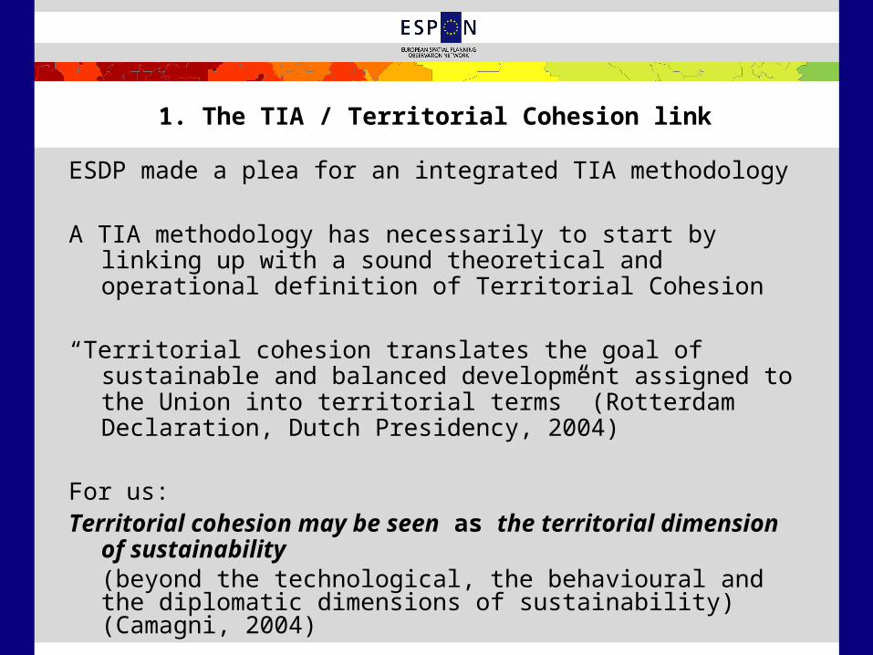
1. The TIA / Territorial Cohesion link

ESDP made a plea for an integrated TIA methodology

A TIA methodology has necessarily to start by linking up with a sound theoretical and operational definition of Territorial Cohesion

“Territorial cohesion translates the goal of sustainable and balanced development assigned to the Union into territorial terms” (Rotterdam Declaration, Dutch Presidency, 2004)

For us:Territorial cohesion may be seen as the territorial

dimension of sustainability (beyond the technological, the behavioural and the diplomatic dimensions of sustainability) (Camagni, 2004)

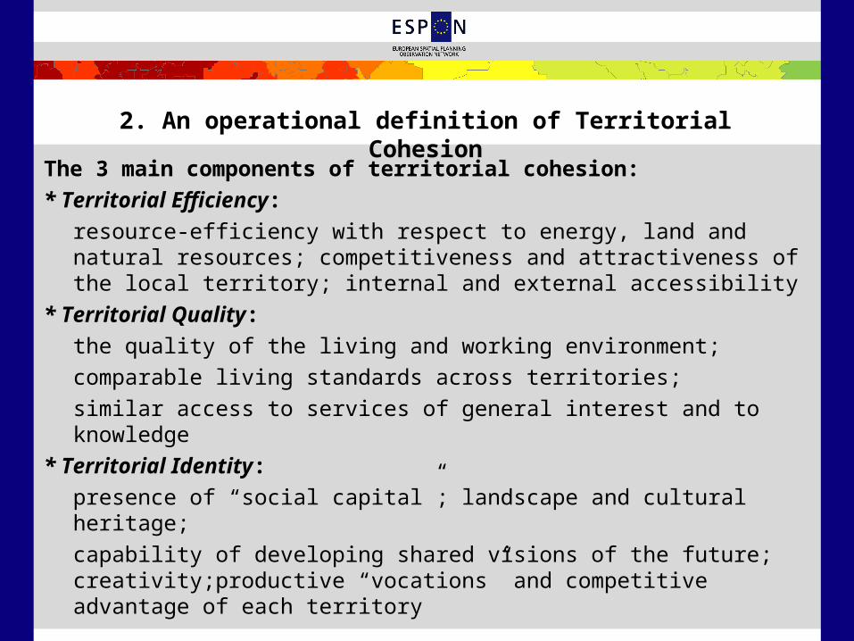
2. An operational definition of Territorial Cohesion

The 3 main components of territorial cohesion:* Territorial Efficiency:

resource-efficiency with respect to energy, land and natural resources; competitiveness and attractiveness of the local territory; internal and external accessibility

* Territorial Quality: the quality of the living and working environment; comparable living standards across territories; similar access to services of general interest and to knowledge

* Territorial Identity: presence of “social capital”; landscape and cultural heritage;capability of developing shared visions of the future; creativity;productive “vocations” and competitive advantage of each territory

2. An operational definition of Territorial Cohesion

3. Territorial dimensions and assessment criteria

Territorial efficiency:

Lisbon:- Economic efficiency and production capability - Competitiveness and innovation capability- Inter-regional integrationGothenborg + Kyoto:- Resource efficiency: consumption of energy, land, water….- Reduction of technological and environmental risk- Compact city form, reduction of sprawlSpatial structure:- Polycentric urban system- Development of city-networks and medium cities- General accessibility - internal and external- Quality of transport and communication services

3. Territorial dimensions and assessment criteria

Territorial quality:

People and cohesion:- Access to services of general interest- Quality of life and working conditions- Multiethnic solidarity and integration- Reduction of interregional income disparities- Reduction of unemployment, poverty and exclusionNatural resources- Conservation and creative management of natural resources- Sustainable transport: public transport and absence of

congestionSpatial structure:- Cooperation between city and coutryside

3. Territorial dimensions and assessment criteria

Territorial identity:

Heritage and landscape- Conservation and creative management of cultural heritage- Conservation and creative management of landscape Production “vocations”- Cognitive capability: creativity and innovativeness- Development of region-specific know-how and knowledge- Accessibility to global knowledge and creative “blending”

with local knowledgeCapabilities- Development of shared “visions” for the futureSocial capital- Cooperation capability; social networks; - Shared behavioural rules

4. The Territorial Assessment Model: the TEQUILA Model

T erritorialE fficiencyQU ality

I dentity the TEQUILA ModelL ayeredA ssessmentModel (Camagni, 2006)

1. TEQUILA is a Multicriteria Model for the Territorial Impact Assessment of EU policies

2. The 3 components of the T.C. concept and their sub-components become the criteria in the Assessment Model

4. The Territorial Assessment Model: the TEQUILA Model

3. The weights of the 3 criteria and sub-criteria are flexible (sensitivity of results with respect to change in weights is

tested interactively)

4. The general impact of EU policies on each criterion is defined using ad hoc studies, with both qualitative and quantitative approaches

5. A method for combining quali-quantitative impact indicators inside the multi-criteria analysis is supplied

4. The Territorial Assessment Model: the TEQUILA Model

Alternative scaling of quantitative assessments (e.g.)

+5

0

180 250 180 250 Impact on regional employment Impact on regional employment

+3

+2

a) “local scaling” b) “ad hoc scaling”

Qualitative impact scores are attributed on a +5 to -5 scale: 5= very high advantage for all; -5= very high disadvantage for all4= high advantage for all; -4= high disadvantage for all3= high advantage for some, med. adv. for all; -3= high disadv. for some, medium disadv. for all2= medium advantage; -2= medium disadvantage1= low advantage; -1= low disadvantage 0= nil impact;

4. The Territorial Assessment Model: the TEQUILA Model

The 2 layers1st layer: General Assessment of the impact of EU policies on

the overall European territory: to be intended as a “potential impact” on an abstract territory (PIM)

2nd layer: “Territorial Assessment” on each region: why?

- the intensity of the policy application may be different on different regions

- the relevance of the different “criteria” is likely to be different for different regions, according to their utility function

- the vulnerability and the receptivity of the different regions to similar “potential” impacts is likely to be different

- a region may not be subject to a specific policy

5. The Territorial Assessment Model: TIM

TIMr = Σc θc . (PIMr,c . Sr,c )

TIM = territorial impactc = criterion of the multi-criteria method r = regionθc = weight of the c criterionPIMr,c = potential impact according to quantitative assessm.Sr,c = sensitivity of region r to criterion c

Sr,c = Dr,c . Vr,cDr,c = desirability of criterion c for region r (territorial “utility

function”)Vr,c = vulnerability of region c to impact on c (receptivity for

positive impacts)

In qualitative assessment: PIMr,c = (PIMc . PIr ) where PIr = policy intensity in r

6. TEQUILA SIP: an Interactive Simulation Package

The TEQUILA model is operated through an interactive simulation device, specifically built for Espon (3.2):

TEQUILA SIP- interactive, easy to build and operate- working on different layers (particularly: Europe 29 and

NUTS 3) and on any EU policy

As a pioneering and prototype experiment, TEQUILA SIP was applied to the assessment of the Territorial Impact of EU transport policy (TEN-TINA), using existing quantitative ESPON assessments and data base

Territorial level : NUTS 3 (1329 regions) Collaboration of ESPON teams in data supply is gratefully

acknowledged

7. Application to TENs policies

3 criteria Variables 9 sub-criteria

PIM_E1 Internal Connectivity

Territorial Efficiency PIM_E2 External Accessibility

PIM_E3 Economic Growth

PIM_Q1 Congestion

Territorial Quality PIM_Q2 Emissions

PIM_Q3 Transport sustainability

PIM_I1 Creativity

Territorial Identity PIM_I2 Cultural heritage

PIM_I3 Landscape resources

7. Application to TENs policies: PIM

PIM Sub-criteria

Indicator Unit of measure Dir Var. Wgt Source of data

PIM_E1InternalConnectivity

Dif transport endowment (road + rail)/GDP

Km / GDP + 0 to 4 0,333ESPON 3.2Mcrit

PIM_E2ExternalAccessibility

Dif accessibility potential (road/rail pass. trav.), scenario B1 (only priority projects) Number of people + 2 to 5 0,333

ESPON 1,2,1 SASI; Mcrit

PIM_E3 GrowthDif GDP per capita, scenario B1 – Difference to reference scenario 2000 – 2021

Dif % GDP/inhabitant + 2 to 4 0,333ESPON 2,1,1, SASI Model

PIM_Q1 Congestion Dif-flows, baseline scenario 2015 Million Vehicles/Km - 2 to -5 0,333ESPON 3.2Mcrit

PIM_Q2 Emissions Dif CO2 emissions baseline Million Tons CO2 / Year - 2 to -5 0,333ESPON 3.2Mcrit

PIM_Q3Transport sustainability

Dif rail - Dif road, baseline scenario 2000-2015

Km - Km + -3 to 3 0,333ESPON 3.2Mcrit

PIM_I1 CreativityDif accessibility*[knowledge and creative services]

(# people)*( # libraries + theatres)

+ 1 to 4 0,333ESPON 2,1,1, SASI Model

PIM_I2Cultural heritage

Dif accessibility*[ # monuments + museums ]

(# people)*( # monuments-museums)

+ 1 to 4 0,333ESPON 2,1,1, SASI Model

PIM_I3 LandscapeDif. Transport endowment (road+rail) / GDP

Km / GDP - 0 to -4 0,333ESPON 3.2Mcrit

7. Application to TENs policies: sensitivitySensitivity Sensitivity parameters Unit of measure Variation Functional

shape Source of data

S_E1

D = LOG of current density of transport endowment [density=(road+rail)/GDP]R = 1S = D norm

LOG[km road+rail] / GDP 0,8 to 1,2 Linear ESPON 3.2McritESPON 3.1

S_E2D = LOG [current accessibility]R = 1S = D norm

LOG [# of people daily accessible by car]

0,8 to 1,2 Non Linear ESPON 2,1,1 – SASI Model

S_E3D = GDP 2000 PPP per inhabitantR = 1S = D norm

GDP 2000 PPP per inhabitant] 0,9 to 1,2 Linear ESPON 3.1, Eurostat Regio

S_Q1D=Present congestion V=Share of natural areasS= mean of normalised D and V

D= Million Vehicles / network KmV= share of natural areas (Km2)

0,8 to 1,2 D = Non Linear ESPON 3.2 –Mcrit; BBR Corine Landcover

S_Q2D=Present emissionsV=Share of natural areas S= mean of normalised D and V

Present emissions CO2 year 2000 [million tons] V= share of natural areas (Km2)

0,8 to 1,20,9 to 1,2

D = Non LinearV = Linear

ESPON 3.2 -McritBBR Corine Landcover

S_Q3D=Present share of railw. on total tran. ntw.R = 1S = D norm

Km / Km (%) 0,8 to 1,2 D = Non Linear ESPON 3.2Mcrit

S_I1D=GDP 2000 PPP per inhabitantR = 1S = D norm

GDP 2000 PPP per inhabitant 0,9 to 1,2 Linear ESPON 3.1, Eurostat Regio

S_I2D=GDP 2000 PPP per inhabitantR = 1S = D norm

GDP 2000 PPP per inhabitant 0,9 to 1,2 Linear ESPON 3.1, Eurostat Regio

S_I3

D=1V = Natural vulnerability (natural area fragmentation)S= V norm

Natural area fragmentation indicator 1-5: 1= very low; 5 = max fragmentation

1,2 to 0,9 LinearESPON 1,3,1; GTK

8. The interactive package

8. The interactive package

8. The interactive package: Impact on Efficiency

8. The interactive package: PIM on accessibility

9. Mapping results: impact on Territorial Efficiency

9. Mapping results: impact on Territorial Quality

9. Mapping results: impact on Territorial Identity

9. Mapping results: General Impact

Beyond TEQUILA: another sip?

a. Improving theory- cause-effect chains: unintentional side-effects of policies- territorial preferences and utility functions

b. Improving modelling effort- Interregional spillover effects (economic, environmental)

c. Enlarging data base- construction/destruction of territorial capital: a paradigm

shift in territorial accounts

d. Picking the right policies: as selective as possible! Avoid complex policies (such as cohesion policy). Better: competitiveness pol., excellence pol., infrastr., capacity building, water managm. policies).

THANKS

As the EU Ministers stated at the end of the Leipzig Charter:

“we look ahead with confidence”

Thanks for your attention!

Roberto CamagniDipartimento di Ingegneria GestionalePolitecnico di MilanoPiazza Leonardo da Vinci 32 - 20133 MILANOtel: +39 02 2399.2744  - 2750 secr.fax: +39 02 2399.2710roberto.camagni@polimi.ithttp://econreg.altervista.org