essays in financial economics - cmu
TRANSCRIPT

DISSERTATION
Essays in Financial Economics
Presented by
EMILIO BISETTI
Submitted to the Tepper School of Business
in partial fulfillment of the requirements for the degree of
Doctor of Philosophy
at
CARNEGIE MELLON UNIVERSITY
April 2018
Dissertation Committee:
Burton Hollifield (Co-Chair)
Stephen A. Karolyi
Stefan Lewellen
Pierre Jinghong Liang
Chris Telmer
Ariel Zetlin-Jones (Co-Chair)

c© Emilio Bisetti 2018ALL RIGHTS RESERVED

Acknowledgments
I am deeply indebted to Burton Hollifield, Ariel Zetlin-Jones, and Chris Telmer, for their endlesssupport and guidance throughout the years. They taught me much of what I know about research,economics, and finance. They spent countless hours listening to, discussing, and helping me de-velop my research ideas. They always treated me as a colleague and a friend, and never stoppedencouraging me to do better.
I am extremely grateful to Steve Karolyi and Stefan Lewellen for their invaluable energy and support.The first chapter of this dissertation greatly improved in quality and depth thanks to their selflesshelp, and they have been fantastic mentors during my job market.
I thank Laurence Ales and Finn Kydland for organizing Macro-Finance PhD workshops and stimu-lating a collaborative research environment between Tepper PhD students. I am also grateful to themany Tepper faculty who generously offered their time to provide feedback to my work. I am parti-cularly grateful to Pierre Liang for serving in my dissertation committee.
I thank my friends and fellow PhD students for years of intense work and fun. In particular, I thankHakkı Ozdenoren, Alex Schiller, and Ben Tengelsen, for endless conversations about economics andfinance. Both the content of my research and my ability to communicate my research to others havegreatly benefited from these conversations. I am especially grateful to Lawrence Rapp and Laila Leefor their invaluable assistance with administrative matters.
I consider myself lucky for having such wonderful friends outside of work as Giorgio Antongio-vanni; Alessandro Biggi; Francesco Brachetti; Ciprian Domnisoru; Daniela Frattini; Christian Frem;Maria Pia Guffanti; Francesco Maccarana; Fulvio Mazza; Andrea Mazzanti; Giacomo Meo; FrancescoMorandi; Marie-Lou and Dana Nahhas; Fares Nimri; Nicola Paccanelli; Pietro Pollichieni; CristinaSangaletti; Andrea Tremaglia; and Dario Zocchi. Their friendship has been essential for me to succeedin graduate school.
Finally, I am truly grateful to Jana for her love and for her patient support during the last years ofmy doctorate. My biggest thanks goes to family for listening to, understanding, and supporting meat every step of my life. This dissertation is dedicated to them.
i

A Silvia, Paolo,Alberto, e Francesco.

Abstract
In the first essay, I address the current debate on the costs and benefits of financial regulation, andI show that financial regulation can increase bank shareholder value by reducing shareholder moni-toring costs. I use a regression discontinuity design to study the effect of an unexpected decrease insmall-bank reporting requirements to the Federal Reserve. Using the reporting change as a negativeshock to regulatory monitoring by the Fed, I find that reduced Fed monitoring leads to a 1% lossin Tobin’s q and a 7% loss in equity market-to-book. I show that these losses come from increasedinternal monitoring expenditures, managerial rents, and monitoring conflicts between shareholders.My results are among the first to quantify the shareholder value of monitoring.
In the second essay (with Benjamin Tengelsen and Ariel Zetlin-Jones), we re-examine the importanceof separation between ownership and labor in team production models that feature free riding. Insuch models, conventional wisdom suggests an outsider is needed to administer incentive schemesthat do not balance the budget. We analyze the ability of insiders to administer such incentive sche-mes in a repeated team production model with free riding when they lack commitment. Specifically,we augment a standard, repeated team production model by endowing insiders with the ability toimpose group punishments which occur after team outcomes are observed but before the subsequentround of production. We extend techniques from Abreu (1986) to characterize the entire set of perfect-public equilibrium payoffs and find that insiders are capable of enforcing welfare enhancing grouppunishments when they are sufficiently patient.
In the third essay, I re-examine an important prediction of asset pricing theory which has historicallyfound little support in the data—that expected consumption growth and equity returns should becorrelated. I first show empirically that advertising growth is a good proxy for expected consumptiongrowth, as it predicts both consumption growth and equity returns in aggregate post-war US data.To shed light on the link between advertising growth, expected consumption, and expected returns, Ithen build and calibrate a dynamic model of goods market frictions where firms invest in advertisingto build their customer capital (as in Gourio and Rudanko (2014)). Within the model, I show that theseverity of goods market frictions is a key element to replicate the predictability patterns I observe inthe data.
iii


Contents
Acknowledgments i
Abstract iii
1 The Value of Regulators as Monitors: Evidence from Banking 1
1.1 Introduction . . . . . . . . . . . . . . . . . . . . . . . . . . . . . . . . . . . . . . . . . . . 2
1.2 Institutional Background and Motivating Theory . . . . . . . . . . . . . . . . . . . . . . 6
1.2.1 Institutional Background . . . . . . . . . . . . . . . . . . . . . . . . . . . . . . . 6
1.2.2 Predictions from Agency Theory . . . . . . . . . . . . . . . . . . . . . . . . . . . 7
1.3 Empirical Setting . . . . . . . . . . . . . . . . . . . . . . . . . . . . . . . . . . . . . . . . 11
1.3.1 Data Sources and Measurement . . . . . . . . . . . . . . . . . . . . . . . . . . . 11
1.3.2 Estimation Strategy and Identification . . . . . . . . . . . . . . . . . . . . . . . . 15
1.4 The Value of Regulatory Monitoring . . . . . . . . . . . . . . . . . . . . . . . . . . . . . 18
1.4.1 Main Results . . . . . . . . . . . . . . . . . . . . . . . . . . . . . . . . . . . . . . 18
1.4.2 Robustness, Placebo, and Falsification Tests . . . . . . . . . . . . . . . . . . . . . 21
1.5 How does Regulatory Monitoring Benefit Shareholders? . . . . . . . . . . . . . . . . . 23
1.5.1 Bank Value, Monitoring Expenditure, and Managerial Rents . . . . . . . . . . . 23
1.5.2 Regulatory Monitoring and Shareholder Free-Riding . . . . . . . . . . . . . . . 30
1.6 Discussion and Tests of Alternative Hypotheses . . . . . . . . . . . . . . . . . . . . . . 32
1.7 Conclusion . . . . . . . . . . . . . . . . . . . . . . . . . . . . . . . . . . . . . . . . . . . . 35
v

vi CONTENTS
2 Group Punishments without Commitment 37
2.1 Introduction . . . . . . . . . . . . . . . . . . . . . . . . . . . . . . . . . . . . . . . . . . . 38
2.2 A Generalized Model of Repeated Team Production . . . . . . . . . . . . . . . . . . . . 42
2.2.1 Stage Game . . . . . . . . . . . . . . . . . . . . . . . . . . . . . . . . . . . . . . . 42
2.2.2 Infinitely-Repeated Game . . . . . . . . . . . . . . . . . . . . . . . . . . . . . . . 46
2.3 An Application: Repeated Oligopoly with a Principal . . . . . . . . . . . . . . . . . . . 57
2.3.1 Stage Game . . . . . . . . . . . . . . . . . . . . . . . . . . . . . . . . . . . . . . . 57
2.3.2 Infinitely-Repeated Game . . . . . . . . . . . . . . . . . . . . . . . . . . . . . . . 59
2.3.3 Substitutability and Price Externalities . . . . . . . . . . . . . . . . . . . . . . . 62
2.4 Conclusion . . . . . . . . . . . . . . . . . . . . . . . . . . . . . . . . . . . . . . . . . . . 65
3 Advertising, Consumption, and Asset Prices 67
3.1 Introduction . . . . . . . . . . . . . . . . . . . . . . . . . . . . . . . . . . . . . . . . . . . 68
3.2 Aggregate Advertising Expenditures and Equity Returns . . . . . . . . . . . . . . . . . 71
3.2.1 Consumption Growth and Excess Returns Predictability . . . . . . . . . . . . . 72
3.2.2 Robustness . . . . . . . . . . . . . . . . . . . . . . . . . . . . . . . . . . . . . . . 78
3.3 Model . . . . . . . . . . . . . . . . . . . . . . . . . . . . . . . . . . . . . . . . . . . . . . . 83
3.3.1 Firm Problem and Return on Equity . . . . . . . . . . . . . . . . . . . . . . . . . 86
3.3.2 Household Problem . . . . . . . . . . . . . . . . . . . . . . . . . . . . . . . . . . 89
3.3.3 Equilibrium . . . . . . . . . . . . . . . . . . . . . . . . . . . . . . . . . . . . . . . 90
3.4 Results . . . . . . . . . . . . . . . . . . . . . . . . . . . . . . . . . . . . . . . . . . . . . . 91
3.4.1 Calibration and Computation . . . . . . . . . . . . . . . . . . . . . . . . . . . . 91
3.4.2 Simulated Moments and Predictability . . . . . . . . . . . . . . . . . . . . . . . 92
3.4.3 The Quantitative Impact of Goods Market Frictions . . . . . . . . . . . . . . . . 93
3.5 Conclusion . . . . . . . . . . . . . . . . . . . . . . . . . . . . . . . . . . . . . . . . . . . . 96

CONTENTS vii
A Appendix to Chapter 1 99
A.1 Solving for the Optimal Contract . . . . . . . . . . . . . . . . . . . . . . . . . . . . . . . 100
A.2 Additional Results: Bank Value . . . . . . . . . . . . . . . . . . . . . . . . . . . . . . . . 101
A.3 Additional Results: Management Monitoring . . . . . . . . . . . . . . . . . . . . . . . . 106
A.4 Tests of Additional Hypotheses . . . . . . . . . . . . . . . . . . . . . . . . . . . . . . . . 115
B Appendix to Chapter 2 119
B.1 Substitutability and Price Externalities . . . . . . . . . . . . . . . . . . . . . . . . . . . 120
B.1.1 Stage Game . . . . . . . . . . . . . . . . . . . . . . . . . . . . . . . . . . . . . . . 120
B.1.2 Infinitely-Repeated Game . . . . . . . . . . . . . . . . . . . . . . . . . . . . . . . 121
B.2 Definitions and Proofs . . . . . . . . . . . . . . . . . . . . . . . . . . . . . . . . . . . . . 124
B.2.1 Definitions and Proofs from Sections 2.2 and 2.3 . . . . . . . . . . . . . . . . . . 124
B.2.2 Proofs from Appendix B.1 . . . . . . . . . . . . . . . . . . . . . . . . . . . . . . . 131
B.3 Computational Algorithm . . . . . . . . . . . . . . . . . . . . . . . . . . . . . . . . . . . 137
C Appendix to Chapter 3 139
C.1 Cointegration Tests . . . . . . . . . . . . . . . . . . . . . . . . . . . . . . . . . . . . . . . 140
C.2 Advertising Expenditures and Long-Run Risk . . . . . . . . . . . . . . . . . . . . . . . 142
C.3 Derivation of the Stochastic Discount Factor . . . . . . . . . . . . . . . . . . . . . . . . . 144
C.4 Computational Algorithm . . . . . . . . . . . . . . . . . . . . . . . . . . . . . . . . . . . 144


List of Tables
1.1 Summary Statistics . . . . . . . . . . . . . . . . . . . . . . . . . . . . . . . . . . . . . . . 13
1.2 The Policy Effect on Bank Shareholder Value . . . . . . . . . . . . . . . . . . . . . . . . 19
1.3 Robustness and Placebo Tests: Tobin’s q . . . . . . . . . . . . . . . . . . . . . . . . . . . 22
1.4 The Policy Effect on Bank Professional Expenditure . . . . . . . . . . . . . . . . . . . . 24
1.5 Professional Expenditure Growth and Post-Treatment Value Losses . . . . . . . . . . . 26
1.6 Managerial Rents: Earnings Smoothing in the Financial Crisis . . . . . . . . . . . . . . 29
1.7 Cash Flow Risk, Shareholder Value, and Professional Expenditures . . . . . . . . . . . 30
1.8 Ownership, Management Monitoring, and Value . . . . . . . . . . . . . . . . . . . . . . 31
3.1 Summary Statistics for Predictors, Post-War Period . . . . . . . . . . . . . . . . . . . . 76
3.2 Consumption Growth and Excess Returns Predictability, Post-War Period . . . . . . . 77
3.3 Excess Returns Predictive Regressions, Post-War Period . . . . . . . . . . . . . . . . . . 78
3.4 Tri-Variate Excess Returns Predictive Regressions, Post-War Period . . . . . . . . . . . 79
3.5 VAR Model for Advertising and Consumption Growth, Post-War Period . . . . . . . . 80
3.6 VAR Model for Advertising and Consumption Growth, 1922-2009 and 1982-2009 . . . 81
3.7 Consumption Growth Predictive Regressions, Post-War Period . . . . . . . . . . . . . 82
ix

x LIST OF TABLES
3.8 Out-of-Sample Excess Returns Predictive Regressions . . . . . . . . . . . . . . . . . . . 85
3.9 Model-Simulated Moments . . . . . . . . . . . . . . . . . . . . . . . . . . . . . . . . . . 93
3.10 Results: Returns Predictability . . . . . . . . . . . . . . . . . . . . . . . . . . . . . . . . . 94
3.11 Predictability in the Centralized Economy . . . . . . . . . . . . . . . . . . . . . . . . . . 96
A1 Robustness and Placebo Tests: Market-to-Book . . . . . . . . . . . . . . . . . . . . . . . 101
A2 Bank Size Manipulation Tests . . . . . . . . . . . . . . . . . . . . . . . . . . . . . . . . . 102
A3 Event Study Around Policy Date . . . . . . . . . . . . . . . . . . . . . . . . . . . . . . . 102
A4 Additional Robustness . . . . . . . . . . . . . . . . . . . . . . . . . . . . . . . . . . . . . 103
A5 Quarterly Treatment Effects . . . . . . . . . . . . . . . . . . . . . . . . . . . . . . . . . . 104
A6 Falsification Tests: Non-Fed-Regulated Firms . . . . . . . . . . . . . . . . . . . . . . . . 105
A7 Triple Differences: Policy Effect on Market-to-Book . . . . . . . . . . . . . . . . . . . . 106
A8 Audit Fees . . . . . . . . . . . . . . . . . . . . . . . . . . . . . . . . . . . . . . . . . . . . 107
A9 Internal Controls and Post-Treatment Professional Expenditure . . . . . . . . . . . . . 108
A10 SEC Accelerated Filers . . . . . . . . . . . . . . . . . . . . . . . . . . . . . . . . . . . . . 109
A11 Summary Statistics: Funding Costs, Profitability, and Earnings Smoothing . . . . . . . 110
A12 Funding Costs and Earnings Smoothing: Robustness and Placebo . . . . . . . . . . . . 111
A13 Robustness: Cash Flow Risk, Shareholder Value, and Professional Expenditure . . . . 112
A14 Chairman Ownership and Professional Expenditure Persistence . . . . . . . . . . . . . 113
A15 Chairman Ownership and Market-to-Book Discount Persistence . . . . . . . . . . . . . 114
A16 Government Tail Risk Insurance . . . . . . . . . . . . . . . . . . . . . . . . . . . . . . . 115
A17 Voluntary Reporting . . . . . . . . . . . . . . . . . . . . . . . . . . . . . . . . . . . . . . 116
A18 Liquidity, Volatility, and Market Frictions . . . . . . . . . . . . . . . . . . . . . . . . . . 117
A19 Leverage and Capital Ratios . . . . . . . . . . . . . . . . . . . . . . . . . . . . . . . . . . 118
C1 Philips-Ouliaris and Johansen Tests for Cointegration . . . . . . . . . . . . . . . . . . . 141
C2 Vector-Error-Correction Model for Consumption Growth Predictions, Post-War Period 142

List of Figures
1.1 Common Trends in Pre-Policy Bank Valuation . . . . . . . . . . . . . . . . . . . . . . . 17
1.2 Bank Size Manipulation . . . . . . . . . . . . . . . . . . . . . . . . . . . . . . . . . . . . 18
2.1 Equilibrium Value Sets and Group Punishments . . . . . . . . . . . . . . . . . . . . . . 62
2.2 Input Substitutability and the Welfare Impact of Group Punishments . . . . . . . . . . 64
3.1 Expenditures in Physical and Non-Physical Advertising in the U.S., 1950-2010 . . . . . 72
3.2 Per-Capita Consumption and Advertising in the U.S., 1950-2010 . . . . . . . . . . . . . 73
3.3 Advertising Expenditures Growth, Consumption Growth and Excess Returns in theU.S., 1950-2010 . . . . . . . . . . . . . . . . . . . . . . . . . . . . . . . . . . . . . . . . . . 74
3.4 Coefficient Estimates in Out-of-Sample Excess Returns Predictive Regressions, 1980-2010 84
3.5 Customer Capital Investment . . . . . . . . . . . . . . . . . . . . . . . . . . . . . . . . . 95
B1 Comparative Statics: Marginal Cost of Production and Welfare . . . . . . . . . . . . . . 124
xi

Chapter 1
The Value of Regulators as Monitors:Evidence from Banking
1

2 CHAPTER 1. THE VALUE OF REGULATORS AS MONITORS: EVIDENCE FROM BANKING
1.1 Introduction
A common view in the banking industry is that financial regulation has a negative impact on share-
holder value: regulatory compliance subtracts resources from lending and deposit-making activities,
reduces profits, and ultimately hurts investors. As a result, the recent decline of small and medium-
sized banks in the United States has often been attributed to regulation, and regulatory burden re-
duction for small banks is now a priority on the agenda of the US Federal Reserve (the Fed). In a
recent testimony to the House Financial Services Committee, the Chair of the Fed Board of Gover-
nors Janet Yellen stated: “With respect to small and medium-sized banks, we must build on the steps we have
already taken to ensure that they do not face undue regulatory burdens.”1 While the current policy discus-
sion highlights the costs of financial regulation for bank investors, agency theory suggests a positive
role for regulation in reducing the costs incurred by shareholders to monitor bank mangement.
In this paper, I exploit the regulatory environment of US Bank Holding Companies (BHCs) to study
the value impact of regulatory monitoring.2 The US Federal Reserve (the Fed) is the primary re-
gulator of BHCs, and a pervasive component of the Fed’s monitoring activity is the collection and
analysis of BHC financial statements. Both the frequency and the volume of BHC reporting to the
Fed are based on a fixed asset size threshold, such that smaller BHCs falling below the threshold are
exempted from most of the reporting requirements faced by larger BHCs above the threshold. I use
a 2006 Fed policy raising this size threshold as a shock to regulatory monitoring, and study changes
in bank value around the new threshold in a regression discontinuity design. My identification stra-
tegy comes from the quasi-random assignment of treated banks just below the threshold and control
banks just above the threshold before the Fed implements its policy, such that any systematic value
difference after the policy implementation is only due to differences in regulatory monitoring.
Following the predictions of agency theory, I interpret the change in Fed regulatory monitoring as a
shock to shareholder monitoring costs. To provide a structure to my empirical tests, I build a stylized
model of monitoring in the class of Townsend (1979), and derive three key predictions on the impact
1Yellen (2016).2Even if a BHC can include more than one bank, I will use the two terms interchangeably in the rest of the paper.

1.1. INTRODUCTION 3
of monitoring costs on shareholder value. In the model, a manager has private incentives to mis-
report bank cash flows and a shareholder can pay a monitoring cost to verify the cash flows reported
by the manager. When monitoring costs are small, the shareholder always monitors and extracts
the entire surplus from the bank. As monitoring becomes more expensive (as for treated banks),
shareholder value drops due to increased monitoring expenditures and increased managerial rents.
The first model prediction is therefore that reduced regulatory monitoring should lead to shareholder
value losses.
My main finding is consistent with the first prediction of the model: I show that, relative to control
banks, treated banks experience a 1% decrease in Tobin’s q (the market value of bank assets divided
by the book value of bank assets) and a 7% decrease in Market-to-Book (the market-to-book value of
bank equity) after the treatment. The finding is robust across a number of empirical specifications,
sample restrictions, placebo tests, and falsification tests. For example, the treatment effect is stronger
around the policy implementation date and threshold and disappears when I use arbitrary placebo
dates and thresholds to separate treatment and control groups, reducing sample selection concerns.
Moreover, my estimate of the treatment effect is not driven by pre-existing differences in valuation
across treated and control groups, and it is not biased by pre-treatment size manipulation.3 Impor-
tantly, the finding is not driven by changes in government bailout guarantees (Gandhi and Lustig
(2015)), financial disclosure (Hutton, Marcus, and Tehranian (2009)), stock liquidity and volatility,
and other size-based regulations implemented by the Fed at the beginning of 2006.
The second model prediction is that the value losses experienced by treated banks should be due
to increased monitoring expenditures and increased managerial rents. In line with this prediction,
I show that treated banks experience a 25% increase in their professional expenditures after the tre-
atment. These professional expenditures are largely related to bank internal controls, and strongly
correlated with post-treatment losses in shareholder value. Moreover, during the financial crisis
banks below the policy implementation threshold engage in more aggressive earnings smoothing
than banks above the threshold, confirming the prediction of increased managerial rents (Fudenberg
3Reporting exemptions are based on June 2005 BHC assets, but the threshold change is first announced by the Fed onlyin November 2005. Additionally, McCrary (2008) tests show no evidence of pre-treatment asset size manipulation.

4 CHAPTER 1. THE VALUE OF REGULATORS AS MONITORS: EVIDENCE FROM BANKING
and Tirole (1995)). Specifically, banks below the threshold decrease their Loan Loss Provisions (LLPs)
by more than banks above the threshold, and these LLP changes are due to managerial discretion
rather than to bank performance.
The third model prediction is that value losses and monitoring expenditures in treated banks should
both be positively correlated with the risk of their unobservable cash flows. Intuitively, high cash
flow risk increases the likelihood of tail states where cash flows are low or managerial rents are high,
decreasing bank value and increasing the marginal value of monitoring. Empirically, I proxy the risk
of unobservable cash flows with the absolute difference between analyst-forecasted and realized
bank profitability. I find that treated banks with high cash flow risk experience larger value losses
and professional expenditure growth than banks with low expected cash flow risk.
Finally, I argue that the increased monitoring costs faced by treated banks’ shareholders increase their
incentives to free-ride on each other’s monitoring (Grossman and Hart (1980), Holmstrom (1982)).
Consistent with Shleifer and Vishny (1986), the presence of a large shareholder—the board chair-
man—helps to mitigate shareholder free-riding problems after the treatment. I show that treated
banks with high chairman ownership experience higher professional expenditure growth and larger
value losses than treated banks with low chairman ownership. Moreover, post-treatment professi-
onal expenditure growth is more persistent and value drops are less persistent in banks with high
chairman ownership.
Overall, my paper is among the first to quantify the shareholder value of monitoring. Quantitatively,
I attribute around sixty percent of the loss in shareholder value for deregulated banks to increased
monitoring expenditure and managerial rents, and I attribute around forty percent of the loss to
increased free-riding problems. I conclude that regulation can be value-increasing for shareholders
when regulators monitor the management. My results are potentially applicable to other heavily-
regulated industries besides the banking industry, and provide new evidence against the standing
consensus that financial regulation negatively affects bank shareholders.

1.1. INTRODUCTION 5
Related Literature A long-standing question in financial economics is the extent to which moni-
toring affects shareholder value. Motivated by theoretical arguments (Shleifer and Vishny (1986),
Kahn and Winton (1998), Maug (1998)), the literature has traditionally focused on institutional ow-
nership as a measure of monitoring to estimate the impact of monitoring on firm value (McConnell
and Servaes (1990), Ferreira and Matos (2008)). Causal inference is however difficult in these studies,
because firm ownership and value are endogenously determined by firms’ contracting environment
(Himmelberg, Hubbard, and Palia (1999), Coles, Lemmon, and Meschke (2012)). My paper contribu-
tes to this literature by using a novel identification strategy to estimate a large and positive impact of
monitoring on value. To the best of my knowledge, my paper is the first to test the predictions of a
traditional class of monitoring models (Townsend (1979), Gale and Hellwig (1985)), and among the
first to show that monitoring is valuable because it reduces managerial rent-seeking.4
Theoretical and emprical research shows that agency frictions are particularly severe in the context of
banking. The risk profile of bank assets is difficult to observe by outsiders and easy to modify by in-
siders (Morgan (2002), Dang, Gorton, Holmstrom, and Ordonez (2017)), and deposit insurance gives
bank lenders low incentives to monitor the management (Gorton and Pennacchi (1990)). Moreover,
deposit insurance and other bank regulations might distort shareholder incentives to take risk (Mer-
ton (1977)), possibly in contrast with managerial preferences (Saunders, Strock, and Travlos (1990)).
Previous empirical work has argued that agency frictions and managerial rent-seeking can have a
negative impact on bank value (Laeven and Levine (2007), Goetz, Laeven, and Levine (2013)). My
work provides causal evidence on the impact of agency frictions on bank value, and demonstrates
regulatory monitoring as an effective tool to mitigate these frictions.
The recent crisis has stimulated academic interest in the costs and benefits of financial regulation.
While many papers show that financial regulation is positively related to bank efficiency (Barth, Lin,
Ma, Seade, and Song (2013)), and negatively related to bank risk-taking and failure (Agarwal, Lucca,
Seru, and Trebbi (2014), Hirtle, Kovner, and Plosser (2016), Kandrac and Schlusche (2017)), a recent
4In this respect, my results are close to Bertrand and Mullainathan (2003), Kempf, Manconi, and Spalt (2016), andSchmidt and Fahlenbrach (2017), who focus on different outcome variables to show that monitoring reduces rent-seeking.Falato, Kadyrzhanova, and Lel (2014) show a positive impact of monitoring on firm value, but are silent about the specificmechanism through which monitoring increases value.

6 CHAPTER 1. THE VALUE OF REGULATORS AS MONITORS: EVIDENCE FROM BANKING
study by Buchak, Matvos, Piskorski, and Seru (2017) shows that bank regulatory burden is one of
the main reasons for the raise of shadow banking. My paper adds to this literature by providing the
first estimate of the value of monitoring by financial regulators.
1.2 Institutional Background and Motivating Theory
The banking industry provides an ideal laboratory to study the impact of regulatory monitoring on
shareholder value. A common view in the banking industry is that regulatory burden is particularly
detrimental to bank profitability and value, and financial regulation is a commonly-cited reason
for the decline of small banks in the United States. This view gained momentum among financial
authorities since the Dodd-Frank Act of 2010, and small bank regulatory burden reduction is now
an important priority on the policymaker’s agenda (Yellen (2016)). While the costs and benefits of
financial regulation are yet not fully understood, agency theory predicts that financial regulation can
have a positive impact on bank value by reducing shareholder monitoring costs.
1.2.1 Institutional Background
The Bank Holding Company Act of 1956 broadly defines a BHC as any company that owns and/or
has control over one or more banks. Commercial banks in the United States are not mandated to
be part of a BHC structure. However, being part part of a BHC offers substantial benefits, such as
increased flexibility in raising external financing and acquiring other banks, as well as the ability to
acquire non-bank subsidiaries. In practice, these benefits are such that at the end of 2016 around
eighty-four percent of commercial banks in the US were part of a BHC.5
The benefits of being part of a BHC come at the cost of compliance with the regulatory and supervis-
ory requirements imposed by the Fed. From a regulatory standpoint, Regulation Y from 1980 gives
the Fed exclusive jurisdiction in establishing BHC capital requirements, regulating BHC mergers
5https://www.fedpartnership.gov/bank-life-cycle/grow-shareholder-value/bank-holding-companies.

1.2. INSTITUTIONAL BACKGROUND AND MOTIVATING THEORY 7
and acquisitions, and defining and regulating non-banking activities performed by BHC subsidia-
ries. From a supervisory standpoint, Section 5 of the Bank Holding Company Act provides guidance
for the off-site and on-site inspections regularly conducted by regional Fed officials under delegated
authority from the Board.
The main information source for Fed off-site inspections is a set of financial statements collected
and reviewed by the Fed on a regular basis. In practice, specialized teams of Fed officials focus on
the analysis and cross-bank comparison of these statements to monitor the safety and soundness of
individual banks, and to identify potential threats to the financial system (Eisenbach, Haughwout,
Hirtle, Kovner, Lucca, and Plosser (2017)). The process through which the Fed collects financial sta-
tements is different for large and small BHCs. Large BHCs need to file every quarter consolidated
financial statements (form FR Y-9C) and holding parent company statements (FR Y-9LP) which con-
tain detailed balance sheet, income statement, and off-balance sheet information about the bank’s
activity. To avoid reporting burden, the Fed allows smaller BHCs to only file an annual statement
for the holding parent company (FR Y-9SP), such that small BHCs face substantially lower reporting
requirements than large BHCs.
The Fed separates small and large reporting BHCs based on a fixed, bank-independent asset size
threshold. From 1986 until the end of 2005, this size threshold was set to $150 million in total assets.
In March 2006, the Fed implemented a regulation increasing the threshold to $500 million (regulation
71-FR-11194), therefore providing new reporting exemptions to all BHCs with assets between $150
and $500 million. I use this change in reporting requirements as a shock to the monitoring costs of
deregulated banks’ shareholders.
1.2.2 Predictions from Agency Theory
What kind of responses can be expected following a shock to shareholder monitoring costs? In this
section I use the lens of a classic model of monitoring (Townsend (1979)) to derive three key testable
predictions and provide structure to the empirical tests of the rest of the paper.

8 CHAPTER 1. THE VALUE OF REGULATORS AS MONITORS: EVIDENCE FROM BANKING
There are two agents in the model, a penniless manager and a shareholder with deep pockets. The
manager and the shareholder are both risk-neutral, and the risk-free rate is zero. The manager has
monopoly access to a project with cost I, which will generate a random cash flow y ∈[
¯y, y]⊆ R+
with cdf F and pdf f at the end of the period. The project has positive NPV, which I denote by Vf :
Vf =∫ y
¯y
ydF (y)− I > 0. (1.1)
The manager costlessly observes the realized project cash flow, and must report the cash flow to
shareholder. The manager can consume the difference between the realized cash flow and the cash
flow that she reports to the shareholder, and therefore has an incentive to under-report to the share-
holder. On the other hand, the shareholder can pay an audit cost k to perfectly observe the realized
cash flow.
The shareholder has full bargaining power, and her problem is to maximize her expected profits
while eliciting truthful cash flow revelation by the manager. Resorting to the revelation principle, I
characterize contracts in which the manager always reveals the true cash flow. A contract is then a
couple {π (y) , m (y)} that specifies payments from the manager to the shareholder π (y) :[
¯y, y]→
R and monitoring decisions m (y) :[
¯y, y]→ {0, 1} as functions of the cash flow reported by the
manager. I assume that audits are deterministic, in the sense that for all y, m (y) is either 0 or 1. This
partitions the set[
¯y, y]
in a region where the shareholders always audits the manager and a region
where the shareholder never audits the manager.
The shareholder maximizes her expected profits
∫ y
¯y[π (y)−m (y) k] dF (y)− I, (1.2)
subject to the manager’s participation constraint
∫ y
¯y[y− π (y)] dF (y) ≥ 0, (1.3)
the manager’s limited liability constraint that, for all y,
y ≥ π (y) , (1.4)

1.2. INSTITUTIONAL BACKGROUND AND MOTIVATING THEORY 9
and the incentive-compatibility constraints ensuring that the manager always reveals the true cash
flow. For the contract to be incentive-compatible, the following conditions must be verified. First, in
the non-monitoring region the shareholder must always receive a constant payment P.6 This allows
to write the payment π (y) as
π (y) = (1−m (y)) P + m (y)π1 (y) , (1.5)
where π1 (y) is the payment in the monitoring region. Second, to prevent the manager to report cash
flows in the non-monitoring region when the observed cash flow is in the monitoring region, it must
be that
m (y)π1 (y) ≤ P. (1.6)
Constraints (1.5) and (1.6) characterize incentive-compatibility by the manager. The shareholder’s
problem then becomes finding m (y) and π1 (y) to maximize her expected profits, subject to con-
straints (1.3)-(1.6).
In the appendix, I solve for the optimal contract. As in Gale and Hellwig (1985), the optimal contract
is such that the monitoring region is the low cash flow region for which π (y) = y < P, and the non-
monitoring region is the high cash flow region for which y ≥ π (y) = P. In the monitoring region, the
shareholder pays the monitoring cost k and the manager gives all the cash flow to the shareholder.
In the non-monitoring region, the shareholder receives the fixed payment P and the manager keeps
y− P.
Finally, conditional on the optimal contract, the optimal fixed payment P∗ is chosen by the sharehol-
der to solve the unconstrained maximization problem
maxP
∫ P
¯y
(y− k) dF (y) + P (1− F (P))− I. (1.7)
6If for some cash flow realization in the monitoring region the contract specifies a lower payment to the shareholderthan for other realizations in the monitoring region, there is an incentive for the manager to report the cash flow associatedwith the lower payment.

10 CHAPTER 1. THE VALUE OF REGULATORS AS MONITORS: EVIDENCE FROM BANKING
Taking the first-order conditions of this problem and re-arranging, I get
1− F (P∗) = k f (P∗) , (1.8)
showing that at the optimum, the shareholder balances the benefits of increasing P coming from
reduced managerial rents with the costs coming from increased monitoring.
The first testable prediction of the model therefore comes from inspection of Equation (1.8), by noting
that as the monitoring cost k becomes small, the probability F (P∗) that the shareholder monitors the
manager approaches one. In other words, when monitoring is inexpensive the shareholder always
monitors and extracts the entire NPV from the project.
Prediction 1. An increase in shareholder monitoring costs leads to shareholder value losses.
Next, let Vc denote shareholder value when monitoring is costly (i.e. k > 0):
Vc =∫ P∗
¯y
(y− k) dF (y) + P∗ (1− F (P∗))− I. (1.9)
The loss in shareholder value from a world where monitoring is costless and the shareholder extracts
the entire project NPV is then
Vf −Vc = kF (P∗) +∫ y
P∗(y− P∗) dF (y) , (1.10)
which consists of monitoring expenditures and managerial rents.
Prediction 2. When shareholder monitoring costs increase, losses in shareholder value are due to increased
monitoring expenditure and managerial rents.
The last model prediction requires assumptions on the distribution of bank cash flows. To provide
intuition, I assume that cash flows are uniformly distributed over the interval[
¯y, y]. The model
generates similar predictions for other types of distributions (e.g. lognormal). Using a uniform
distribution, some simple algebra shows that the shareholder value loss (1.10) becomes
Vf −Vc = k
(1− 1
2k
y−¯y
), (1.11)

1.3. EMPIRICAL SETTING 11
which is increasing in the term y −¯y. Noting that expected monitoring expenditure, kF (P∗), is
also increasing in y−¯y, and that y−
¯y is proportional to cash flow risk, the last prediction directly
follows.7
Prediction 3. When shareholder monitoring costs increase, shareholder value losses and monitoring expendi-
ture are increasing in cash flow risk.
Intuitively, when cash flow risk increases the likelihood of states where income is low or managerial
rents are high increases, and this reduces shareholder value relative to a world where monitoring is
costless and the manager cannot extract any rents. Over the next few sections I show that regulatory
monitoring reduces shareholder monitoring costs by testing the predictions of my stylized model in
the data.
1.3 Empirical Setting
In this section I describe how I measure bank value, monitoring expenditure, and cash flow risk
in the data, and describe how I use these variables to estimate the shareholder value of regulatory
monitoring.
1.3.1 Data Sources and Measurement
The data on BHC total consolidated assets comes from the Federal Reserve Regulatory Dataset. This
dataset is publicly available on the Federal Reserve of Chicago’s website, and contains information
directly coming from the FR Y-9C, FR Y-9LP, and FR Y-9SP reports. I use the dataset to categorize
BHCs into treated and control groups based on their 2005 average consolidated assets, and to keep
track of which BHCs file which forms in each quarter.8 Since the Fed policy allows treated banks to
stop reporting their FR Y-9C consolidated statements, I use Compustat Bank as my main source of
7The standard deviation of a uniform distribution with support [a, b] is given by (b− a) /√
12.8This is important because, as I show in Section 1.6, some BHCs voluntarily keep filing forms FR Y-9C and FR Y-9LP
even if their total assets are below $500 million after the treatment.

12 CHAPTER 1. THE VALUE OF REGULATORS AS MONITORS: EVIDENCE FROM BANKING
BHC consolidated financial data. I combine this dataset with CRSP to obtain end-of-quarter BHC
market-to-book values, and in turn merge the Compustat-CRSP combined dataset with the Federal
Reserve Regulatory Dataset using the link table available on the Federal Reserve of New York’s
website. Finally, I obtain data on analyst forecasts of bank profitability from I/B/E/S.
The observation frequency is quarterly, starting with the first quarter of 2004 and ending with the
last quarter of 2007. Within this time period, I construct my main sample as follows. I focus on top-
tier BHCs (defined as in Goetz, Laeven, and Levine (2016)) with average 2005 total assets between
$150 and $850 million, and with stock price data available on CRSP. I assign individual BHCs to the
treated group if their average total assets in 2005 are between $150 million and $500 million, and to
the control group if their average total assets in 2005 are between $500 million and $850 million.9
The final sample consists of 2,780 observations on 208 distinct BHCs, out of which 108 belong to the
treated group and 100 belong to the control group. These BHCs represent around ten percent of the
total number of BHCs in the US at the end of 2005, and around forty-six percent of the BHCs listed
on the stock market at the end of 2005. In terms of size, these banks represent around one percent of
the total assets in the banking sector at the end of 2005, and around five percent of the assets in the
bottom ninety-nine percent of the asset distribution. Finally, the average pre-treatment BHC asset
size in my sample is $519 million, right above the policy implementation threshold.
Table 1.1 reports summary statistics for my main measures of bank value, monitoring expenditure,
and cash flow risk, both in the full sample and in the treated and control sub-samples.10 The first
two rows of Panel A show summary statistics for my measures of bank shareholder value, Tobin’s
q and the Market-to-Book ratio of bank equity. The data shows little dispersion in these valuation
ratios, both within the main sample and across the treated and control sub-samples. The average
and median Tobin’s q in the main sample are 1.07 and 1.06, respectively, and the average and median
Market-to-Book are 1.75 and 1.65.
9I choose the upper bound of $850 million in total assets in such a way that the final treated and control samples containapproximately the same number of banks. In Section 3.2.2, I use $1 billion and $1.5 billion as alternative upper bounds,and show that the main results of the paper are not sensitive to these choices.
10Since I only observe evidence of managerial rents during the financial crisis, I leave a description of how I measurethese rents to Section 1.5.1.

1.3. EMPIRICAL SETTING 13
Table 1.1
Summary Statistics
This table reports summary statistics for the variables in the paper, both in the main sample and in the treatedand control sub-samples. In Panel A, Tobin’s q is the market value of total assets (market value of equityplus book value of debt) divided by the book value of total assets. Market-to-Book is the market value ofequity divided by the book value of equity. Professional Services are fees paid to management consultingfirms, investment banks, and auditing firms, in millions of US dollars. Cash flow risk is a quarterly averageof the absolute difference between monthly analyst consensus forecast of two-year-forward bank EPS and therealized EPS value corresponding to each consensus forecasts. In Panel B, leverage is total liabilities divided bytotal assets, Tier 1 Ratio is Tier 1 Capital divided by Risk-Weighted Assets, Profitability is net income dividedby net interest income, and ROE is net income divided by book value of equity. Total Assets are reported inmillions of US dollars. Finally, diversification is non-interest income divided by net interest income, and assetgrowth is quarterly growth in BHC total assets.
Panel A: Shareholder Value, Monitoring Expenditure, and Cash Flow Risk
Full Sample Treated Control
N Mean Med. SD N Mean Med. SD N Mean Med. SD
Tobin’s q 2,623 1.07 1.06 0.05 1,329 1.06 1.06 0.05 1,294 1.07 1.06 0.05Market-to-Book 2,623 1.75 1.65 0.57 1,329 1.71 1.60 0.57 1,294 1.80 1.72 0.56Professional Fees 1,756 0.14 0.10 0.16 862 0.13 0.10 0.14 894 0.16 0.12 0.18Cash Flow Risk 937 0.87 0.24 2.38 306 1.54 0.34 3.80 631 0.55 0.22 1.04
Panel B: Additional Variables
Full Sample Treated Control
N Mean Med. SD N Mean Med. SD N Mean Med. SD
Leverage 2,624 0.91 0.91 0.03 1,329 0.91 0.91 0.03 1,295 0.91 0.91 0.02Tier 1 Ratio 2,289 0.12 0.12 0.03 1,096 0.13 0.12 0.04 1,193 0.12 0.11 0.03Total Assets 2,703 554.9 535.6 232.5 1,341 386.5 382.8 128.5 1,362 720.6 696.8 188.8Profitability 2,701 0.23 0.26 0.34 1,340 0.20 0.24 0.44 1,361 0.25 0.27 0.19ROE 2,624 0.02 0.03 0.03 1,329 0.02 0.02 0.03 1,295 0.03 0.03 0.02Diversification 2,701 0.27 0.22 0.24 1,340 0.26 0.20 0.29 1,361 0.27 0.24 0.18Asset Growth 2,655 0.03 0.02 0.06 1,308 0.03 0.02 0.06 1,347 0.03 0.02 0.05

14 CHAPTER 1. THE VALUE OF REGULATORS AS MONITORS: EVIDENCE FROM BANKING
The third row of Panel A shows summary statistics for bank professional expenditures, in millions
of US dollars. These expenditures are recorded as a separate item on bank income statements, and
include fees paid to consultants, auditors, and investment bankers. In Section 1.5.1, I show that
professional expenditures are a good proxy for shareholder monitoring in my sample, because they
are mostly related to the implementation of internal controls. Banks in the treated group pay slightly
lower professional fees than banks in the control group. On average, treated banks spend 0.13 million
of dollars per quarter in professional services, with a standard deviation of 0.14 million. Control
banks spend on average 0.16 million of dollars per quarter in professional services, with a standard
deviation of 0.18 million.
The last row of Panel A finally presents my primary cash flow risk measure, the absolute difference
between analyst consensus forecast of two-year-forward bank EPS and the realized EPS value corre-
sponding to each consensus forecast. By construction, this variable provides a time-varying measure
of analyst uncertainty about future bank profitability, and therefore represents a close approximation
to the risk of unobservable cash flows in my model. The table shows that cash flow risk is on average
higher for treated banks than for control banks, partially reflecting lower analyst coverage of small
banks. Both before and after the treatment, the average treated bank is covered by approximately
four analysts analysts in a given quarter, while the average control bank is covered by six analysts.
Panel B of Table 1.1 reports summary statistics for the other key variables in the paper, which I
borrow from the literature as potential determinants of cross-sectional heterogeneity in bank value
(Laeven and Levine (2007), Minton, Stulz, and Taboada (2017)). These variables include leverage
(total liabilities minus noncontrolling interest divided by total assets), the regulatory Tier 1 Regula-
tory Capital Ratio (henceforth Tier 1 Ratio, the bank self-reported ratio of Tier 1 Capital divided by
Risk-Weighted Assets), total assets, profitability (net income divided by net interest income), Return
on Equity (ROE, net income divided by book value of equity), diversification (noninterest income
divided by net interest income), and quarterly asset growth. As in Panel A, the data reveals little
differences in these variables across treated and control groups, thus confirming the comparability
of these two sets of banks.

1.3. EMPIRICAL SETTING 15
1.3.2 Estimation Strategy and Identification
In this section, I describe my strategy to test the model predictions in the data and to measure the
shareholder value of regulatory monitoring. I exploit the change in regulatory reporting require-
ment to the Fed as a quasi-natural source of variation in shareholder monitoring costs. My empiri-
cal strategy consists in comparing the value and monitoring expenditure of smaller, treated banks
with pre-treatment total assets just below $500 million with the value of larger, control banks with
pre-treatment total assets just above $500 million, before and after the treatment. More precisely, I
estimate the model
Yit = β0 + β1 (Postt × Treatedi) + β2Xit + γi + δt + εit, (1.12)
where Yit is an outcome variable (e.g. Tobin’s q) for BHC i in quarter t, Postt is an indicator equal
to one if quarter t follows the last quarter of 2005 and zero otherwise, Treatedi is an indicator equal
to one if the average assets of BHC i during 2005 are just below $500 million, Xit is a matrix of time-
varying control variables (such as assets and profitability), γi is a time-invariant and BHC-specific
fixed effect, δt is a BHC-invariant and time-specific fixed effect, and εit is a normally-distributed error
term. The coefficient of interest is β1, my estimate of the value difference between treated and control
banks before and after the treatment.
My empirical strategy relies on the key identification assumption of quasi-random assignment of
treated and control banks around the threshold before the Fed changes the reporting requirements of
treated banks, such that any systematic value difference after the policy implementation is arguably
only due to differences in regulatory monitoring. In practice, this assumption can be violated for
two reasons. First, the assumption is violated if the threshold change results from lobbying, making
the treatment an endogenous outcome. Second, the assumption is violated if, even in absence of
lobbying, banks engage in size manipulation around the new threshold before its implementation.
Although the institutional details of the policy suggest that lobbying was unlikely, whether the po-
licy was unanticipated by bank shareholders is ultimately an empirical question.11 In Figure 1.1 I11The first proposal for public comment on the policy dates to November 2005, and the policy was quickly implemented
at the beginning of March 2006 without modifications to the initial proposal.

16 CHAPTER 1. THE VALUE OF REGULATORS AS MONITORS: EVIDENCE FROM BANKING
report a diagnostic test aimed at detecting pre-existing differences in the average valuation of tre-
ated and control banks before the treatment. Panels A and B report these diagnostics for Tobin’s
q and Market-to-Book, respectively, and are constructed as follows. I first divide the sample into
two sub-samples, the pre-treatment sample before the first quarter of 2006 and the post-treatment
sample starting with the first quarter of 2006. In each of these sub-samples, I run a kernel-weighted
local polynomial regression to obtain a smoothed estimate of the trend component of treated and
control banks’ valuation. In Figure 1.1 I then plot these estimated trend components and their as-
sociated confidence intervals as functions of the observation quarter, both in the pre- and in the
post-treatment periods.12 Figure 1.1 shows that the trend components of treated and control banks’
valuation are statistically indistinguishable from each other in the pre-treatment period, supporting
the claim that the threshold change was unanticipated. Moreover, the figure shows an increase in
the difference between treated and control banks’ average valuation after the treatment, providing a
visual preview of the results in the next section.
In Figure 1.2, I report the results of a McCrary (2008) discontinuity test to reduce concerns of bank
size manipulation around the $500 million threshold. Specifically, I construct a finely-gridded his-
togram of bank total assets, which I then smooth on each size of the threshold using local linear
regression. In Figure 1.2, I then report point estimates and 95% confidence intervals of smoothed as-
set densities during the 2005-2007 period (Panel A) and during the four quarters immediately before
the treatment (Panel B). Both before and after the treatment, the estimated asset density below the
threshold is not statistically different from the estimated asset density above the threshold.13 Impor-
tantly, a specific institutional feature of the policy reduces residual concerns of asset manipulation
before the treatment. The policy states that individual BHCs qualify for reporting exemptions only
if their June 2005 consolidated assets are below $500 million. At the same time, the Fed first publicly
announces the threshold change in November 2005, preventing pre-treatment size manipulation.
12I divide the sample to avoid post-treatment observations entering the estimation of the pre-treatment trend, andvice-versa. All panels of Figure 1.1 are constructed using an Epanechnikov kernel and the rule-of-thumb bandwidth sizesuggested in Fan and Gijbels (1996). Different kernel and bandwidth choices generate similar results.
13All the results are calculated using the histogram bin size and local linear regression bandwidth suggested in McCrary(2008).

1.3. EMPIRICAL SETTING 17
Figure 1.1
Common Trends in Pre-Policy Bank Valuation
This figure reports a parallel trends diagnostic test on treated and control banks’ Tobin’s q (Panel A) andMarket-to-Book (Panel B). I first divide the sample into two sub-samples, the pre-treatment sample before thefirst quarter of 2006 and the post-treatment sample starting with the first quarter of 2006. In each of thesesub-samples, I run a kernel-weighted local polynomial regression to obtain a smoothed estimate of the trendcomponent of valuation. The local polynomial regression uses an Epanechnikov kernel and the rule-of-thumbbandwidth suggested in Fan and Gijbels (1996). The figure reports point estimates and 95% confidence in-tervals of the trend component of treated and control banks’ valuation as functions of the estimation quarter.Tobin’s q and Market-to Book are defined as in Table 1.1.
1.02
1.04
1.06
1.08
1.1
Policy Change
2004q1 2005q1 2006q1 2007q1 2008q1
Control 95% C.I.Treated 95% C.I.
Panel A: Tobin's q
1.2
1.4
1.6
1.8
2
Policy Change
2004q1 2005q1 2006q1 2007q1 2008q1
Control 95% C.I.Treated 95% C.I.
Panel B: Market-to-Book Ratio

18 CHAPTER 1. THE VALUE OF REGULATORS AS MONITORS: EVIDENCE FROM BANKING
Figure 1.2
Bank Size Manipulation
This figure shows point estimates and 95% confidence intervals of the smoothed cross-sectional density ofbank total assets during the 2005-2007 period (Panel A) and during the four quarters preceding the Policy(Panel B). The goal of the figure is to detect discontinuities indicative of size manipulation around the Policythreshold. The smoothed densities are obtained by first constructing finely-gridded histograms of the cross-section of bank total assets, and by then smoothing the histograms on each size of the threshold using locallinear regression. The optimal histogram bin size and local linear regression bandwidth are calculated usingthe procedure in McCrary (2008).
0.0
005
.001
.001
5.0
02.0
025
Policy Threshold
0 500 1000 1500 2000Total Assets (USD Millions)
Panel A: 2005-2007 BHC Asset Density
0.0
005
.001
.001
5.0
02.0
025
Policy Threshold
0 500 1000 1500Total Assets (USD Millions)
Panel B: 2005 BHC Asset Density
1.4 The Value of Regulatory Monitoring
In this section I present my main results on the value impact of regulatory monitoring.
1.4.1 Main Results
Table 1.2 shows my main findings on the value impact of regulatory monitoring. The table reports
point estimates for the coefficients in Equation (1.12), along with their standard errors (clustered at
the BHC-level). The main coefficient of interest is associated with the “Post × Treated” term, which
represents an estimate of the percentage change in Tobin’s q and Market-to-Book due to the change
in reporting requirements.
When I estimate Equation (1.12) only including quarter- and BHC-level fixed effects, the policy treat-
ment leads to a one percent decline in treated bank Tobin’s q, relative to control banks. The economic

1.4. THE VALUE OF REGULATORY MONITORING 19
Table 1.2
The Policy Effect on Bank Shareholder Value
This table reports estimates of the treatment effect on bank valuation using the empirical specification in Equa-tion (1.12). The coefficient associated with the “Post × Treated” interaction term captures the percentagechange in treated bank valuation due to the treatment. The table includes year-quarter Fixed Effects (FE)and BHC FE. All the variables are defined as in Table 1.1.
log Tobin’s q log Market-to-Book
(1) (2) (3) (4) (5) (6)
Post × Treated -0.010*** -0.011*** -0.010*** -0.069*** -0.079*** -0.074***(0.00) (0.00) (0.00) (0.03) (0.02) (0.02)
Leverage 0.318*** 0.253** 5.473*** 5.170***(0.12) (0.10) (0.81) (0.68)
Tier 1 Ratio 0.376*** 0.280*** 2.539*** 1.746***(0.08) (0.07) (0.51) (0.48)
log Assets -0.032*** -0.234***(0.01) (0.05)
Profitability -0.004 0.041(0.00) (0.04)
ROE 0.091** 0.292(0.04) (0.47)
Diversification -0.004 -0.054(0.00) (0.04)
Asset Growth -0.006 -0.021(0.01) (0.07)
Year-Quarter FE Yes Yes Yes Yes Yes YesBHC FE Yes Yes Yes Yes Yes YesR-Squared 0.360 0.393 0.418 0.413 0.470 0.503Observations 2,177 2,177 2,177 2,177 2,177 2,177
Note: Standard errors (in parentheses) are clustered at the BHC-level. ***, **, and * respectively denote sta-tistical significance at the 1%, 5%, and 10% levels.

20 CHAPTER 1. THE VALUE OF REGULATORS AS MONITORS: EVIDENCE FROM BANKING
magnitude and statistical significance of the treatment effect are not affected by the inclusion of le-
verage and Tier 1 Ratio, reducing concerns that the effect might be due to contemporaneous changes
in small bank capital requirements (see Section 1.6). Everything else equal, a ten percent increase in
leverage and Tier 1 Ratio are respectively associated to a 3.2 and 3.8 percent increase in Tobin’s q, but
the treatment still induces a 1.1 percent decrease in Tobin’s q after the inclusion of these variables.
Finally, the results are robust to the inclusion of size, profitability, diversification, and asset growth
as additional controls.
In the last three specifications of the table, I repeat the same exercise using Market-to-Book as de-
pendent variable. The table shows that the treatment induces a 6.9 percent loss in Market-to-Book
for treated banks, and this value loss is as high as 7.9 percent when I add time-varying controls to
the specification. To put these numbers in perspective, a seven percent relative decrease in Market-
to-Book corresponds to a $4 million relative decrease in market capitalization for the average treated
bank, implying an aggregate market capitalization loss of approximately $430 million. Finally, a
comparison of the first three and the last three columns of Table 1.2 shows that the treatment effect
on Tobin’s q is almost one order of magnitude smaller than the treatment effect on Market-to-Book.
This is due to leverage, which reduces the impact of equity fluctuations on the market value of bank
assets.14 Overall, the results of the table are consistent with the prediction that increased monitoring
costs reduce bank shareholder value.
14A simple example can illustrate this point. Respectively define by Et, Dt and Mt the book value of equity, the bookvalue of debt and the market value of equity in quarter t. Suppose that Et and Dt do not change between quarter t andquarter t + 1 (i.e. Et = Et+1 ≡ E and Dt = Dt+1 ≡ D), but Mt changes to Mt+1. Let ∆Mt+1 ≡ Mt+1 −Mt. Finally, let mbt andqt respectively define the Market-to-Book ratio and Tobin’s q at time t. The change in Market-to-Book between time t andt + 1 is given by
∆mbt+1 =Mt+1Et+1
− MtEt
=∆Mt+1
E. (1.13)
Then, changes in Tobin’s q can be expressed as a function of changes in Market-to-Book and bank leverage:
∆qt+1 =Mt+1 + Dt+1Et+1 + Dt+1
− Mt + DtEt + Dt
=∆Mt+1E + D
=(
1− DE + D
)∆mbt+1, (1.14)
where the term in parentheses in (1.14) is on average equal to 9% in my sample.

1.4. THE VALUE OF REGULATORY MONITORING 21
1.4.2 Robustness, Placebo, and Falsification Tests
Table 1.3 reports two sets of tests aimed at reducing sample selection concerns. In the interest of
space, I only present results for Tobin’s q, leaving the results for Market-to-Book to the appendix.
In Panel A, I test the impact of different sample bandwidth restrictions on my main result. In the
first four specifications of the table, I use two small samples of BHCs with average 2005 total assets
between $400 and $600 million, and between $300 and $700 million. In the last four specifications,
I conversely use two large samples of BHCs with total assets between $150 million and $1 billion,
and between $150 million and $1.5 billion. To mitigate the impact of confounding factors at the onset
of the financial crisis as the sample size changes, the results in Table 1.3 only include data for 2005
and 2006. The table shows that the main results of the paper are not sensitive to different sample
bandwidth choices. Moreover, the first four specifications—which measure the treatment effect on
banks closest to the threshold—show that the treatment leads to an average 1.2 percent discount in
Tobin’s q, slightly larger than the effect found in Table 1.2.
In Panel B I conversely show that the statistical and economic magnitude of my results disappear
when I separate treated and control banks using arbitrary treatment thresholds and quarters. The
first six specifications show that the results disappear when I use asset thresholds of $300 million,
$750 million and $1 billion to separate treated and control banks. Similarly, Specifications (7) and (8)
show that the results disappear when I use the last quarter of 2004 as treatment quarter, and the last
two specifications show that the results disappear when I use the last quarter of 2006 as treatment
quarter.
In the appendix, I provide additional robustness tests. First, I run an event study to show that the
observed drop in Tobin’s q and Market-to-Book are driven by a drop in the market value of treated
banks as opposed to an increase in their book value or an increase in the market value of control
banks. Second, I apply different restrictions on my sample to include the financial crisis, exclude
banks that drop out of the sample, and exclude banks that are not listed on the stock market before
the policy. Again, my results are robust to these restrictions. Third, I show that the treatment effect
on bank value is roughly uniform at the peak of the business cycle in 2006 and at the beginning of

22 CHAPTER 1. THE VALUE OF REGULATORS AS MONITORS: EVIDENCE FROM BANKING
Table 1.3
Robustness and Placebo Tests: Tobin’s q
This table reports sample bandwidth selection tests (Panel A) and placebo tests (Panel B) on my main Tobin’s qresult. In the first four specifications of Panel A, I use two small samples of BHCs with average 2005 total assetsbetween $400 and $600 million (Specifications (1) and (2)), and between $300 and $700 million (Specifications(3) and (4)). In the last four specifications, I use two large samples of BHCs with total assets between $150 mil-lion and $1 billion (Specifications (5) and (6)), and between $150 million and $1.5 billion (Specifications (7) and(8)). In the first six specifications of Panel B, I use asset thresholds of $300 million, $750 million and $1 billionto separate treated and control BHCs. In Specifications (7) and (8) I use the last quarter of 2004 as treatmentquarter, dropping post-2005 observations from the sample. In the last two specifications, I use the last quarterof 2006 as treatment quarter. The dependent variable in all specifications is the natural logarithm of Tobin’s q.Unreported control variables include leverage, Tier 1 Ratio, total assets, profitability, ROE, diversification, andasset growth.
Panel A: Sample Bandwidth Selection
$400M-600M $300M-700M $150M-1B $150M-1.5B
(1) (2) (3) (4) (5) (6) (7) (8)
Post × Treated -0.012** -0.012** -0.011** -0.012*** -0.010*** -0.012*** -0.011*** -0.012***(0.01) (0.01) (0.00) (0.00) (0.00) (0.00) (0.00) (0.00)
Controls No Yes No Yes No Yes No Yes
Year-Quarter FE Yes Yes Yes Yes Yes Yes Yes YesBHC FE Yes Yes Yes Yes Yes Yes Yes YesR-Squared 0.117 0.169 0.087 0.131 0.058 0.105 0.046 0.089Observations 355 355 724 724 1,313 1,313 1,611 1,611
Panel B: Placebo Tests
$300M Threshold $750M Threshold $1B Threshold After 12/2004 After 12/2006
(1) (2) (3) (4) (5) (6) (7) (8) (9) (10)
Post × Treated -0.00 -0.00 0.00 -0.00 0.00 0.00 0.00 -0.00 -0.00 -0.00(0.01) (0.01) (0.00) (0.00) (0.00) (0.00) (0.00) (0.00) (0.00) (0.00)
Controls No Yes No Yes No Yes No Yes No Yes
Year-Quarter FE Yes Yes Yes Yes Yes Yes Yes Yes Yes YesBHC FE Yes Yes Yes Yes Yes Yes Yes Yes Yes YesR-Squared 0.385 0.459 0.339 0.403 0.360 0.422 0.054 0.146 0.351 0.408Observations 1,056 1,056 1,509 1,509 2,076 2,076 1,028 1,028 2,177 2,177
Note: Standard errors (in parentheses) are clustered at the BHC-level. ***, **, and * respectively denote sta-tistical significance at the 1%, 5%, and 10% levels.

1.5. HOW DOES REGULATORY MONITORING BENEFIT SHAREHOLDERS? 23
the financial crisis in 2007, supporting the validity of my results outside the specific environment of
early 2006. Fourth, using Compustat data I construct two falsification samples of non-financial firms
and non-BHC financial firms (e.g. insurance companies and banks that are not BHCs), and study
whether the valuation of firms with 2005 average total assets just below $500 million changes after
the treatment date, relative to the valuation of firms with total assets just above $500 million. The
results show no evidence of value changes in these falsification samples, confirming that the Fed
threshold change, as opposed to other size-based regulations, drives the drop in treated bank value.
1.5 How does Regulatory Monitoring Benefit Shareholders?
In this section I provide additional evidence for my proposed mechanism by testing the remainng
model predictions, namely that reduced regulatory monitoring increases shareholder monitoring
expenditure and managerial rents, and that bank value losses and monitoring expenditure are po-
sitvely correlated with cash flow risk. Moreover, I show that increased shareholder monitoring costs
increase shareholder incentives to free-ride on each other’s monitoring.
1.5.1 Bank Value, Monitoring Expenditure, and Managerial Rents
The second prediction of the costly state verification model is that the observed losses in treated
bank value should be due to increased shareholder monitoring expenditure and managerial rents.
Table 1.4, provides a first test of this prediction by showing that the policy results in a twenty-five
percent increase in treated bank professional expenditure. This relative professional expenditure in-
crease is economically large for treated banks, amounting to approximately twenty-seven thousand
dollars per quarter or 3.8 percent of the average treated bank’s pre-treatment quarterly net income.
Consistent with the model’s predictions, when I discount these increased professional expenditures
(after-taxes) at an average quarterly ROE of two percent, their discounted present value amounts
to slightly less than a million dollars, around twenty-five percent of the four million relative drop
in market value experienced by the average treated bank. In other words, increased monitoring
expenditures only account for a fraction of the loss in treated bank market value.

24 CHAPTER 1. THE VALUE OF REGULATORS AS MONITORS: EVIDENCE FROM BANKING
Table 1.4
The Policy Effect on Bank Professional Expenditure
This table shows the treatment effect on treated banks’ professional expenditure. In the first three specificationsI use the natural logarithm of professional fees as dependent variable, while in the last three specifications Iuse the natural logarithm of professional fees normalized by net interest income. Additional control variablesnot reported in the table include total assets, profitability, ROE, diversification, and asset growth.
log Professional Fees log Professional FeesNet Interest Income
(1) (2) (3) (4) (5) (6)
Post × Treated 0.259*** 0.267*** 0.244*** 0.225** 0.224** 0.232***(0.09) (0.09) (0.07) (0.09) (0.09) (0.08)
Leverage -2.080 -1.640 2.051 0.885(3.22) (2.49) (3.08) (2.53)
Tier 1 Ratio -4.471*** -2.173 -1.436 -1.290(1.51) (1.34) (1.46) (1.35)
Other Controls No No Yes No No Yes
Year-Quarter FE Yes Yes Yes Yes Yes YesBHC FE Yes Yes Yes Yes Yes YesR-Squared 0.076 0.101 0.182 0.047 0.062 0.129Observations 999 999 999 999 999 999
Note: Standard errors (in parentheses) are clustered at the BHC-level. ***, **, and * respectively denote sta-tistical significance at the 1%, 5%, and 10% levels.

1.5. HOW DOES REGULATORY MONITORING BENEFIT SHAREHOLDERS? 25
Next, in Table 1.5, I show that the post-treatment losses in market value are strongly correlated
with professional expenditures. In practice, I augment the main specification of Table 1.2 with an
interaction term for professional expenditures incurred by treated banks only after the treatment,
capturing the post-treatment correlation between treated bank professional expenditure and value.
In most specifications, I include time-varying risk controls such as Z-Score, equity return volatility,
and a tail risk measure borrowed from Ellul and Yerramilli (2013). The table shows that the statistical
significance of the treatment effect is entirely captured by post-treatment professional expenditures
by treated banks. While the magnitude of this triple-differences estimate has no clear economic inter-
pretation, its significance suggests a strong positive correlation between post-treatment professional
expenditure and losses in shareholder value. Moreover, in the appendix I show that this correlation
does not seem to be mechanically driven by changes in profitability, size, or risk variables that are
potentially correlated with both professional expenditure and value.
Finally, a more in-depth analysis reveals that post-treatment professional expenditure growth for tre-
ated banks is mainly related to increased management monitoring, as opposed to other professional
services such as auditing and investment banking. In the appendix, I show that fees paid to consul-
tants experience a much larger increase after the treatment than fees paid to auditors (from annual
AuditAnalytics). Moreover, when I divide treated banks based on whether their post-treatment 10-K
notes cite internal controls consulting as a component of professional expenditure, the increase in
professional expenditure is larger for treated banks that cite internal controls as a significant source
of expenditure.15
Managerial Rents
In this section I provide empirical support for the hypothesis that reduced monitoring costs increase
managerial rents, where I measure managerial rents by earnings smoothing (Fudenberg and Tirole
(1995)). Specifically, I use the August 2007 rise in money market interest rates as a shock to the
15In many banks, internal controls expenditures are related to Sarbanes-Oaxley (SOX). In the appendix, I show that theobserved decline in treated banks’ valuation is however not due to interactions between the policy and size-related SOXprovisions (see, for example, Iliev (2010)).

26 CHAPTER 1. THE VALUE OF REGULATORS AS MONITORS: EVIDENCE FROM BANKING
Table 1.5
Professional Expenditure Growth and Post-Treatment Value Losses
In this table I study the interaction between post-treatment professional expenditure growth and post-treatment bank value losses. In the table, the term “Post × Treated × Prof. Fees” captures treated banks’professional expenditures that only occur after the treatment. Z-Score is computed as the moving average ofbank capital-asset ratio (book value of equity divided by book value of assets), plus the moving average ofROA, divided by the moving standard deviation of ROA. Moving averages are calculated over a horizon ofthree quarters. Equity Volatility is the quarterly standard deviation of daily equity returns. Tail risk is thenegative of the average return over the 5% worst return days that a bank’s stock experiences in a given quar-ter (Ellul and Yerramilli (2013)). Professional fees are normalized by net interest income. Unreported controlvariables include total assets, leverage, profitability, ROE, diversification, and asset growth.
log Tobin’s q log Market-to-Book
(1) (2) (3) (4) (5) (6)
Post × Treated -0.001 -0.001 -0.000 0.003 -0.000 0.004(0.01) (0.01) (0.01) (0.04) (0.03) (0.03)
Prof. Fees -0.037 -0.067 -0.075* -0.103 -0.244 -0.437(0.05) (0.04) (0.04) (0.52) (0.45) (0.36)
Post × Treated × Prof. Fees -0.139*** -0.105** -0.124** -1.447*** -1.196*** -1.188***(0.05) (0.05) (0.06) (0.54) (0.43) (0.39)
Z-Score 0.000 0.000 0.000 0.000(0.00) (0.00) (0.00) (0.00)
Equity Volatility 1.681*** 1.681*** 11.419*** 10.430***(0.29) (0.25) (1.41) (1.55)
Tail Risk -0.813*** -0.789*** -6.008*** -5.713***(0.11) (0.10) (0.63) (0.54)
Other Controls No No Yes No No Yes
Year-Quarter FE Yes Yes Yes Yes Yes YesBHC FE Yes Yes Yes Yes Yes YesR-Squared 0.290 0.336 0.376 0.368 0.417 0.485Observations 1,641 1,641 1,641 1,641 1,641 1,641
Note: Standard errors (in parentheses) are clustered at the BHC-level. ***, **, and * respectively denote sta-tistical significance at the 1%, 5%, and 10% levels.

1.5. HOW DOES REGULATORY MONITORING BENEFIT SHAREHOLDERS? 27
funding costs of BHCs with total assets around $500 million, and analyze the impact of this negative
shock on managerial earnings smoothing right above and right below the threshold. Since money
market interest rates are determined in the interbank lending market of large banks, non-systemic
banks with assets around $500 million arguably play a negligible role in determining this funding
shock. Any observed difference in funding costs and earnings smoothing of banks right above and
below the threshold should therefore only arise from the different exposure of these banks to Fed
monitoring.
To test whether the 2007 shock has a different impact on banks with assets right above and right
below the threshold, I construct two new groups of treated and control BHCs. The new group of
treated, “unmonitored” BHCs consists of BHCs with less than $500 million in assets during the 2006-
2008 period. The new group of control, “monitored” BHCs consists of BHCs with more than $500
million in assets during the same period. To avoid potential bias due to the change in the definition
of small BHCs, I drop observations before the first quarter of 2006. Moreover, I drop BHCs with
total assets above $700 million such that systemic banks are excluded from the sample and such that
the unmonitored and monitored groups have roughly the same number of banks (sixty-seven and
fifty-seven, respectively). My results are not sensitive to this sample bandwidth choice.
In Table 1.6 I report my main results on the impact of Fed supervision on funding costs, profitability,
and earnings smoothing during the crisis.16 Panel A shows the impact of Fed supervision on the
funding costs and profitability of unmonitored banks relative to monitored banks. In the first two
specifications of Panel A, I use total interest expense divided by total loans as a measure of BHC
funding costs. The table shows that during the crisis the difference between the cost of funding of
unmonitored and monitored banks increases by 5.3 percent relative to the pre-crisis period, and that
this effect is robust to the inclusion of lagged Tobin’s q, leverage, Tier 1 Ratio, total assets, diver-
sification and asset growth as regression covariates. The next specifications show that this relative
increase in unmonitored bank funding costs is however not associated with an increase in interest
revenue (interest income divided by total loans), and only by a marginally significant decrease in
16Summary statistics for the dependent variables used in this section are reported in the appendix.

28 CHAPTER 1. THE VALUE OF REGULATORS AS MONITORS: EVIDENCE FROM BANKING
ROE. As a result, unmonitored banks’ higher funding costs must be followed by higher noninterest
revenue, lower noninterest expense, or both.
In the first two specifications of Panel B, I show that unmonitored bank Loan Loss Provisions—a
component of noninterest expense—indeed experience a large decline during the financial crisis.
While the results of the baseline Specification (1) are not statistically significant, the second specifica-
tion of Panel B shows that during the crisis unmonitored bank LLPs decrease by fifty-three percent
relative to monitored bank LLPs after controlling for size, profitability, and other sources of bank
heterogeneity. The observed decline is not due to bank size or performance, and is therefore consis-
tent with the hypothesis of earnings smoothing (as previously documented by Huizinga and Laeven
(2012)). In the last four specifications of Panel B, I confirm this hypothesis by showing a relative in-
crease in small bank Discretionary Negative Loan Loss Provisions (DNLLPs) during the crisis. These
discretionary provisions are the absolute negative residuals from a first-stage regression of LLP on
observable performance variables, and measure the negative change in LLP that is not due to bank
performance (Kanagaretnam, Lim, and Lobo (2014)). Panel B shows a relative DNLLPs increase as
large as seventy percent for unmonitored banks, confirming that the decline in LLP documented in
the first two specifications is due to managerial discretion as opposed to performance.
In the appendix, I conduct additional tests to address potential concerns that the results of Table 1.6
are driven by a subset of small, distressed banks during the crisis rather than by Fed monitoring. In
particular, I show that the results are robust within the sample of banks surviving for the entire 2006-
2008 period, and lose economic and statistical significance when I choose an alternative threshold of
$400 million to define the two groups of unmonitored and monitored banks.
Cash Flow Risk
In Table 1.7 I test my third prediction that banks with higher cash flow risk should experience a
larger decline in value and a larger increase in monitoring expenditure after the treatment. To do
so, I divide treated banks into two sub-groups based on whether their average cash flow risk (as
defined in Section 1.3.1) is above or below the median cash flow risk in my sample. In the table, I

1.5. HOW DOES REGULATORY MONITORING BENEFIT SHAREHOLDERS? 29
Table 1.6
Managerial Rents: Earnings Smoothing in the Financial Crisis
In this table, I study the impact of Fed monitoring on bank funding costs, profitability, and earnings smoothingduring the financial crisis. In Panel A, I study the change in funding costs (total interest expense dividedby total loans), interest revenue (interest income divided by total loans), and ROE. In Panel B, I study thechange in LLP (loan loss provisions normalized by net interest income) and DNLLP (constructed followingKanagaretnam et al. (2014) as the absolute negative residual from a regression of LLP on previous-quarterloan loss allowance, current-quarter loan charge-offs to assets, loans to assets, non-performing loans to assetsand change in total loans) during the financial crisis. The dependent variable used to calculate DNLLP 1 iscurrent-quarter LLP, while the dependent variable used to calculate DNLLP 2 is previous-quarter LLP. Thesample period is 2006-2008. Unmonitored banks are banks that are below the $500 million threshold for theentire sample period. Unreported controls include previous-quarter Tobin’s q, leverage, the Tier 1 Ratio, totalassets, diversification and asset growth in Panel A, as well as operating profitability and ROE in Panel B.
Panel A: Funding Costs and Profitability
log Int. ExpenseTotal Loans log Int. Income
Total Loans ROE
(1) (2) (3) (4) (5) (6)
Crisis × Unmonitored 0.053** 0.053*** 0.018 0.019 -0.008 -0.003(0.02) (0.02) (0.01) (0.01) (0.01) (0.00)
Controls No Yes No Yes No Yes
Year-Quarter FE Yes Yes Yes Yes Yes YesBHC FE Yes Yes Yes Yes Yes YesR-Squared 0.673 0.755 0.626 0.662 0.184 0.530Observations 899 899 899 899 899 899
Panel B: Loan Loss Provisions
log LLPNet Int. Income log DNLLP 1 log DNLLP 2
(1) (2) (3) (4) (5) (6)
Crisis × Unmonitored -0.359 -0.531*** 0.610** 0.614** 0.704*** 0.708***(0.25) (0.18) (0.25) (0.25) (0.24) (0.24)
Controls No Yes No Yes No Yes
Year-Quarter FE Yes Yes Yes Yes Yes YesBHC FE Yes Yes Yes Yes Yes YesR-Squared 0.286 0.521 0.336 0.351 0.344 0.360Observations 614 614 543 543 549 549
Note: Standard errors (in parentheses) are clustered at the BHC-level. ***, **, and * respectively denote sta-tistical significance at the 1%, 5%, and 10% levels.

30 CHAPTER 1. THE VALUE OF REGULATORS AS MONITORS: EVIDENCE FROM BANKING
then study the treatment effect on value and professional expenditure in these two cash flow risk
groups. The table shows that treated banks with high cash flow risk experience larger value losses
than treated banks with low cash flow risk. For example, the relative loss in Market-to-Book for
treated banks with high cash flow risk is twice as large as the average value loss in the main sample,
while the relative value loss for treated banks with low cash flow risk is not statistically different
from zero. Moreover, treated banks with high cash flow risk also experience a much larger increase
in monitoring expense than treated banks with low cash flow risk, again in line with the predictions
of the model. In the appendix, I finally show that most of the results of the table also hold when
using alternative risk measures such as Z-Scores and equity return volatility.
Table 1.7
Cash Flow Risk, Shareholder Value, and Professional Expenditures
In this table I study the treatment effect on value and professional expenditure for treated banks with above-and below-median cash flow risk, where cash flow risk is defined as in Table 1.1. Unreported control variablesinclude leverage, Tier 1 Ratio, total assets, profitability, ROE, diversification and asset growth.
log Tobin’s q log Market-to-Book log Prof. Fees
(1) (2) (3) (4) (5) (6)
Post × Treated × Low CF Risk 0.001 -0.003 -0.015 -0.021 0.101 0.202**(0.00) (0.01) (0.04) (0.04) (0.10) (0.10)
Post × Treated × High CF Risk -0.018*** -0.014*** -0.152*** -0.114*** 0.421*** 0.338***(0.01) (0.01) (0.04) (0.04) (0.12) (0.08)
Controls No Yes No Yes No Yes
Year-Quarter FE Yes Yes Yes Yes Yes YesBHC FE Yes Yes Yes Yes Yes YesR-Squared 0.373 0.434 0.436 0.525 0.135 0.271Observations 1,547 1,547 1,547 1,547 737 737
Note: Standard errors (in parentheses) are clustered at the BHC-level. ***, **, and * respectively denote sta-tistical significance at the 1%, 5%, and 10% levels.
1.5.2 Regulatory Monitoring and Shareholder Free-Riding
I finally argue that increased shareholder monitoring costs increase their incentives to free-ride on
each other’s monitoring (Grossman and Hart (1980), Holmstrom (1982)). Consistent with the the pre-
dictions of Shleifer and Vishny (1986), I show that the presence of a large shareholder—the chairman
of the board of directors—helps mitigating this free-rider problem and increases bank value.

1.5. HOW DOES REGULATORY MONITORING BENEFIT SHAREHOLDERS? 31
Table 1.8
Ownership, Management Monitoring, and Value
In this table I study the post-treatment interaction between bank ownership, professional expenditure, andvalue, immediately following the treatment. I first assign treated banks to two groups based on whether theirpre-treatment chairman ownership falls in the bottom two terciles (low-ownership) or in the top tercile (high-ownership) of the pre-treatment chairman ownership distribution in my sample. In the table, I then study howdifferent levels of pre-treatment chairman ownership interact with changes in post-treatment professional ex-penditure and value. Since the focus of the table is the short-term treatment effect on professional expenditureand value, my estimates only include data from 2005 and 2006. Quarterly bank ownership data comes fromS&P Capital IQ. Unreported control variables include total assets, leverage, the Tier 1 Ratio, profitability, ROE,diversification, and asset growth.
log Prof. Fees log Prof. FeesNet Int. Income log Market-to-Book
(1) (2) (3) (4) (5) (6)
Post × Treated × Low Chair Own. 0.167* 0.183* 0.188* 0.187* -0.079*** -0.077***(0.09) (0.09) (0.09) (0.10) (0.03) (0.03)
Post × Treated × High Chair Own. 0.521*** 0.512*** 0.416*** 0.477*** -0.028 -0.045*(0.07) (0.06) (0.11) (0.08) (0.05) (0.03)
Controls No Yes No Yes No Yes
Year-Quarter FE Yes Yes Yes Yes Yes YesBHC FE Yes Yes Yes Yes Yes YesR-Squared 0.085 0.149 0.083 0.175 0.055 0.228Observations 368 368 368 368 782 782
Note: Standard errors (in parentheses) are clustered at the BHC-level. ***, **, and * respectively denote sta-tistical significance at the 1%, 5%, and 10% levels.
In Table 1.8, I investigate how different levels of chairman ownership affect monitoring costs and
valuation immediately after the treatment.17 Similar to Table 1.7, I first divide treated banks in two
groups based on whether their pre-treatment ownership by the chairman falls in the bottom two
terciles or in the top tercile of the pre-treatment chairman ownership distribution in my sample. In
the table, I then study the professional spending and value losses in these two groups of banks. The
main objective of this table is to show the short-term treatment effect on professional expenditure
and value for banks with different levels of ownership, and the table therefore only reports results
for the years 2005 and 2006.
The first four specifications show that banks with low and high levels of chairman ownership re-
17Ownership data comes from S&P Capital IQ. The results presented in the table are qualitatively similar, althoughstatistically and economically weaker, for other categories of ownership such as institutional ownership. A possible expla-nation for this result is that the banks in my sample are relatively small compared to other financial institutions, and likelyrepresent a small fraction of institutional investors’ portfolio (Fich, Harford, and Tran (2015)).

32 CHAPTER 1. THE VALUE OF REGULATORS AS MONITORS: EVIDENCE FROM BANKING
spectively increase their professional expenditure by eighteen and fifty-one percent after the tre-
atment. In absolute terms, these relative changes translate into an average twenty-five thousand
dollar increase in professional expenditure for banks with low chairman ownership, and an average
thirty thousand dollar increase for banks with high chairman ownership. Despite the much larger
increase in relative professional expenditure and the slightly larger increase in absolute expenditure,
the last two specifications show that treated banks with high chairman ownership only experience
around sixty percent of the value drop of treated banks with low chairman ownership.18 In other
words, while the discounted present value of bank professional expenditure is approximately the
same across the two ownership groups, the valuation of banks with low chairman ownership drops
by much more than the valuation of banks with high chairman ownership.
Consistent with the idea that ownership resolves shareholder free-riding problems, in the appendix
I finally show that the treatment effect on professional expenditure is not only larger but also more
persistent in banks with high chairman ownership. At the same time, the post-treatment drop in
shareholder value is lower and less persistent for these banks relative to banks with low chairman
ownership.
1.6 Discussion and Tests of Alternative Hypotheses
Collectively, the results of the previous sections suggest that the large value losses of treated banks
are due to increased shareholder monitoring costs. Quantitiatively, the discounted present value of
increased monitoring expenditures accounts for around twenty-five percent of their loss in share-
holder value. Moreover, as just shown in Section 1.5.2, around forty precent of the value loss can
be attributed to free-riding problems as shareholder monitoring becomes more expensive. Follo-
wing the guidance of my model and my previous empirical results, I finally attribute the residual
shareholder value losses to increased managerial rents.
18Pre-treatment valuations in the two ownership groups are not statistically different from each other.

1.6. DISCUSSION AND TESTS OF ALTERNATIVE HYPOTHESES 33
Despite empirical evidence supporting the model’s predictions, my results make it difficult to fi-
nally conclude that the residual shareholder value losses are necessarily due to mangerial rents. My
strategy is to rule out alternative hypotheses that might explain these residual value losses.19
Government Tail Risk Insurance An important question is whether the government provides dif-
ferent degrees of tail risk insurance to small and large banks. If this is the case, part of the discounts
observed in treated bank value might just reflect a loss of government insurance, as opposed to re-
duced Fed monitoring. To test this hypothesis, I construct a daily version of the Gandhi and Lustig
(2015) risk factor capturing aggregate tail risk in US banks’ stock returns. As discussed in their paper,
this size factor is the normal risk-adjusted return on a portfolio that goes long in small bank stocks
and short in large bank stocks, and represents a bank-specific risk factor orthogonal to other equity
and bond factors. In the appendix, I test whether treated banks experience a change in their expo-
sure to bank-specific tail risk after the treatment, where I measure this risk exposure as the quarterly
loading of bank excess returns on the size factor. In practice, I repeat the usual exercise using each
bank’s quarterly loading on the size factor (the estimate from a quarterly time-series regression of
daily bank excess returns on the daily size factor) as dependent variable. My results show no sig-
nificant changes in deregulated banks’ exposure to tail risk, and therefore to government tail risk
insurance.
Financial Statement Disclosure A second possible channel for the residual losses in treated bank
value is reduced financial disclosure (Hutton et al. (2009)). To rule out this hypothesis, I use a policy
provision of the Fed policy allowing treated BHCs to keep filing form FR Y-9C, while also preventing
them to revert to form FR Y-9SP if they choose to do so. Following this provision, I define treated
banks as voluntary filers if they file form FR Y-9C in March 2006 (the first quarter in which the policy
becomes effective).20 In the appendix, I analyze the treatment effect on twenty-nine voluntary filers
19For expositional convenience, the tables relative to this section are confined to the appendix.20The policy gives the Fed the option to determine if a small bank should file form FR Y-9C based on additional indi-
vidual criteria such as diversification. However, this provision is only effective from the second half of 2006 and virtuallynever used by the Fed in subsequent periods.

34 CHAPTER 1. THE VALUE OF REGULATORS AS MONITORS: EVIDENCE FROM BANKING
(the voluntary-reporting group), and compare it to the effect on the remaining treated banks (the not-
reporting group). The treatment effect on each sub-group is a one percent decrease in Tobin’s q, both
in baseline specifications and when I add time-varying controls. Similarly, the treatment induces a
7.7 percent drop in voluntary-reporting BHCs’ Market-to-Book, almost identical to the 7.6 percent
drop for not-reporting BHCs. The results are similar when I add time-varying controls, confirming
that the treatment affects treated banks irrespective of their financial disclosure.
Liquidity, Volatility, and Market Frictions Another possible concern is that the stocks of treated
BHCs become riskier or less liquid following the treatment. Lower information availability might
decrease the liquidity of treated banks’ stocks—therefore justifying an illiquidity premium. Alter-
natively, institutional investors might treat the stocks of small and large banks differently, possibly
using Fed thresholds to define their investment strategy. For example, if many institutional inves-
tors can only hold stocks of large banks, one would expect a decrease in turnover, an increase in
idiosyncratic risk, and a decrease in market information responsiveness for treated banks’ stocks.
My results show no significant changes in the liquidity, volatility, and market information responsi-
veness of treated banks’ stocks after the treatment. More specifically, the data shows no significant
changes in five stock liquidity measures commonly used in the market microstructure literature, na-
mely Effective Tick Size (Holden (2009), Goyenko, Holden, and Trzcinka (2009)), the Corwin and
Schultz (2012) Bid-Ask Spread measure, the Amihud (2002) measure, Zero Days Traded (the number
of days in which a stock is not traded) and Turnover (traded volume divided by shares outstan-
ding). Similarly, the data shows no significant changes in treated banks’ risk profile, where I use
the standard deviation of BHC stock returns to measure total risk and the residual standard devia-
tions from the Fama-French four factor model and the Adrian, Friedman, and Muir (2015) Financial
CAPM model to measure bank idiosyncratic risk. Finally, I find no evidence of changes in stock price
responsiveness to market information, as measured by the delay variables of Hou and Moskowitz
(2005).
Leverage and Capital Requirements I finally analyze the treatment effect on leverage and capital
ratios. The policy closely follows another Fed regulation relaxing the capital requirements of treated

1.7. CONCLUSION 35
BHCs’ parent companies (71 FR 9897). According to this regulation, the parent companies of BHCs
with less than $500 million in total assets (i.e. the parent companies of treated BHCs) are exempted
from regular capital requirements to finance levered acquisitions. Although unlikely (capital requi-
rements exemptions are optional, and the banking subsidiaries of treated BHCs are still subject to
regular capital requirements), there might be a concern that high leverage increases bank default
risk, resulting in lower valuation. The appendix shows that the leverage and the regulatory capital
ratios of treated banks do not change after the treatment.
1.7 Conclusion
In this paper, I use a Fed policy relaxing the reporting requirements of a subset of US banks as a
quasi-natural experiment to investigate the impact of regulatory monitoring on shareholder value.
The paper shows that Tobin’s q and equity market-to-book of deregulated banks respectively fall by
one and seven percent after the policy, and shows that this result is due to an increase in shareholder
monitoring costs when regulatory monitoring decreases. I show that, absent regulatory monitoring,
increased shareholder monitoring costs lead to increased monitoring expenditure, managerial rents,
and free-riding problems between shareholders.
From an economic standpoint, the paper shows that monitoring has a large impact on firm value,
and demonstrates the positive role of regulation in reducing shareholder monitoring costs. From
a policy standpoint, the paper provides an empirical counter-argument to the standing view that
financial regulation is bad for bank investors, especially in small and medium-sized banks. In this
sense, future work should be aimed at measuring the contribution of agency frictions to the value
discounts observed in very large banks (Minton et al. (2017)), and quantifying the costs and benefits
of financial regulation for these large, complex financial institutions.

36 CHAPTER 1. THE VALUE OF REGULATORS AS MONITORS: EVIDENCE FROM BANKING

Chapter 2
Group Punishments without Commitment
37

38 CHAPTER 2. GROUP PUNISHMENTS WITHOUT COMMITMENT
2.1 Introduction
Teams exist in many economic settings, ranging from teams of individuals working together in clubs,
partnerships, or firms, to teams of companies in the form of cartels and lobby groups, to teams of
nations in the form of political alliances and economic unions. In each of these settings, teams aim
to improve outcomes by coordinating efforts across members and are often successful in doing so.
Organizing as a team, however, may also introduce moral hazard problems, especially when team
outcomes are shared and individual effort is not perfectly observed.
In static environments of team production subject to unobservable moral hazard, Holmstrom (1982)
shows the only way to alleviate moral hazard problems is to rely on an outsider who can punish
the entire team after observing an aggregate outcome associated with a deviation by some team
member. Punishments take the form of throwing away some share of the team’s output. Holmstrom
(1982) argues that the intervention of an outsider is also necessary to implement such punishments
in a repeated environment, as the team might not want to enforce these punishments once team
production outcomes are realized: “There is a problem [...] in enforcing such group penalties if they are
are self-imposed by the worker team. [...] Ex post it is not in the interest of any of the team members to waste
some of the outcome. But if it is expected that penalties will not be enforced, we are back in the situation with
budget-balancing, and the free-rider problem reappears.”
In this paper, we ask if and under what conditions outsiders are truly needed to enforce group
punishments in a repeated context. In other words, we ask whether the ability of individual team
members to punish other team members in the future enables the team to enforce group punishments
which occur after aggregate outcomes are realized but before the realization of individual payoffs in
the current period. We call such within-the-period punishments static group punishments. Since these
punishments occur sequentially after individuals choose their private actions, this environment re-
sembles a repeated extensive form game as in Mailath et al. (2017). We obtain a simple characteri-
zation of the set of public perfect equilibrium payoffs and show that, depending on the nature of
the payoffs that agents obtain from team production, the team can indeed enforce static group pu-

2.1. INTRODUCTION 39
nishments. In such cases, the threat of static group punishments is welfare enhancing relative to an
environment in which the team’s action set does not allow for static group punishments.
We start our analysis from a generalized model of repeated team production, featuring a team of
agents and a benevolent Principal—a construct to represent team-wide preferences. In our model,
agents individually choose a level of effort to contribute to the realization of a common outcome.
After observing this common outcome, the Principal chooses a group punishment (possibly zero)
which negatively affects the common outcome. The Principal, like the agents, cannot commit to
a long-term strategy for group punishments. Since the Principal’s action occurs after the common
outcome is observed, the benevolent Principal values period utility of all agents plus the sum of
future discounted stage-game payoffs of all the agents.
Our main contribution is to show that this commonly studied repeated team production environ-
ment admits a simple, recursive characterization for the set of perfect-public equilibria. Specifically,
we show how to characterize the entire equilibrium set of our generalized team production mo-
del using simple “carrot-and-stick” strategies for the worst perfect-public equilibrium (as in Abreu
(1986)). We show that group punishments reduce the gains from deviations in the “carrot” phase,
but increase the gains from deviations in the “stick” phase. Therefore, deviations from the “stick”
never call for immediate implementation of group punishments, further simplifying the recursive
characterization of the equilibrium set.1
Our main findings are that static group punishments can be enforced by the threat of future actions
by team members; and that the threat of static group punishments strictly improves the best attaina-
ble equilibrium welfare relative to an economy where the Principal’s actions are restricted to never
implement group punishments. Moreover, we show that a necessary condition for static group pu-
nishments to improve welfare is the presence of complementarities between aggregate outcomes
and private actions in team members’ stage game payoffs. We show that the total static deviation
payoff (the total payoff that a deviant team member obtains within the deviation period) can be ex-
pressed as the deviant’s static private gain minus a cost to incentivize the Principal to implement
1We argue that imperfect observability plays a key role in our recursive characterization, making continuation payoffsindependent of the identity of the deviator (Mailath et al. (2017)).

40 CHAPTER 2. GROUP PUNISHMENTS WITHOUT COMMITMENT
group punishments. Absent complementarities between aggregate outcomes and private actions,
group punishments have no impact on this total static deviation payoff, and are therefore ineffective
in deterring individual deviations—an outsider a la Holmstrom (1982) is required to improve wel-
fare. Conversely, when team members’ private actions interact with aggregate outcomes group pu-
nishments do reduce the total static deviation payoff by indirectly reducing team members’ private
incentives to deviate. In these cases, group punishments are useful to deter individual deviations,
and an outsider may not be needed to improve welfare.
Our findings in the generalized model indicate that in presence of complementarities between ag-
gregate outcomes and private actions, the Principal who lacks commitment (i.e. the team) might
be capable of replicating incentive schemes which do not satisfy budget balancing without the aid
of outsiders. In the second part of the paper, we apply our generalized team production model to
the repeated oligopoly model of Abreu (1986), and ask which features of producers’ payoffs make
self-imposed group punishments most effective in improving team welfare—and therefore limit the
need for an outsider. In the oligopoly model, team members are producers individually choosing
how much output to produce, and the team outcome is the common price faced by all producers (a
decreasing function of aggregate team output). On the other hand, the group punishment imposed
by the Principal is a tax rate (possibly zero) which has the effect of reducing the price of producers’
output. As in the generalized model, the Principal cannot commit to a long-term strategy for taxes.
Within the context of the oligopoly model, we first show that group punishments imposed by the
Principal are particularly effective in increasing team welfare for intermediate levels of the produ-
cers’ discount factor. Intuitively, when producers are very impatient the threat of future punishments
is weak and only small group punishments can be sustained following static deviations. For inter-
mediate levels of the discount factor, the team can sustain large enough static group punishments
such that the threat of these punishments allows the team to achieve the socially-optimal level of
production. When producers are very patient, the threat of future punishments is strong enough
that the team can sustain the socially-optimal level of production even without resorting to group
punishments. Second, we show that for a given level of the discount factor group punishments are

2.1. INTRODUCTION 41
more effective when producers’ output is highly substitutable. In these cases, deviations by indi-
vidual producers have a small impact on the common price, increasing producers’ static incentives
to deviate, and increasing the ability of group punishments to improve team welfare relative to an
economy where group punishments are not part of the team’s action set.
Related Literature Our paper is related to a large literature concerning moral hazard in static team
production settings. Alchian and Demsetz (1972) describe the opportunity for team members to shirk
and still receive compensation and the need for a principal to prevent shirking. Holmstrom (1982)
suggests a particular kind of contract in which a principal withholds payment whenever output is
below its socially optimal level. Other studies solve the moral hazard problem by injecting a de-
gree of competition among team members via tournaments, rankings, or other relative performance
measures (see Hart and Holmstrom (1986) for a survey).
One of the main challenges in taking these static team production games to the infinitely-repeated
domain is to characterize the set of perfect-public equilibrium payoffs. Mailath et al. (2017) show
that in a wide range of extensive-form games (including team production games) the equilibrium
set cannot be characterized using simple penal codes, because both within-period punishments and
continuation payoffs need to fit the identity of the deviator after a deviation has occurred. In our
paper, we assume that group punishments can only affect team outcomes (due to imperfect observa-
bility), and show how under this assumption the equilibrium set can be characterized using simple
penal codes. In other words, we show that simple penal codes can be used to characterize the entire
set of perfect-public equilibrium payoffs in a broad set of repeated extensive-form games featuring
imperfect observability.
An alternative to group punishments is to allow agents to make side payments to each other (Goldlucke
and Kranz (2012, 2013)). This arrangement avoids costly forms of retaliation when an agent deviates,
and yet is still incentive-compatible since the non-deviant agent receives a positive money transfer
from the deviant. Harrington and Skrzypacz (2007, 2011) describe how the lysine and citric acid car-
tels successfully used these types of contracts, and employed monitors to audit the money-transfer

42 CHAPTER 2. GROUP PUNISHMENTS WITHOUT COMMITMENT
process. This class of models offer a recursive characterization of the equilibrium set using simple
penal codes, but is limited to teams of two agents or settings in which individual actions are obser-
vable.
More in general, our analysis is concerned with team production when a static game is repeated for
infinitely many periods. In this setting, agents have an opportunity to retaliate against the team in
future periods if shirking is detected (Fudenberg and Maskin, 1986; Ostrom et al., 1992). Moreo-
ver, in repeated settings enforcing the aforementioned mechanisms of peer evaluations and relative
performance rankings can become strategic problems in their own right, as exemplified by Che and
Yoo (2001), Fuchs (2007), and Cheng (2016). Finally, our question bears some similarity to the “Who
will guard the guardians?” question examined in Hurwicz (2008), Rahman (2012), Aldashev and
Zanarone (2017), and Acemoglu and Wolitzky (2015) among others. Our setup differs slightly in that
the guardian is the team itself, and individual team members must be willing to retaliate against the
team when group punishments are not enforced.
2.2 A Generalized Model of Repeated Team Production
We begin by describing a model of repeated team production where a benevolent Principal can im-
pose group punishments after observing aggregate deviations. We provide conditions under which
the Principal’s ability to impose static group punishments—defined as punishments that occur after
aggregate output is observed, but before currrent-period payoffs are realized—can be sustained in
equilibrium to increase the welfare of the team. Moreover, if team members are sufficiently patient,
the threat of these punishments can strictly increase team welfare relative to an environment where
the Principal’s actions are restricted to never implement group punishments.
2.2.1 Stage Game
A team consists of n agents indexed by i = 1, . . . , n.2 Each agent chooses an unobservable and non-
negative action ai ∈ R+, representing a level of effort. The cost of action ai is given by c(ai), where2In what follows, we use the terms “agents”and “team members” interchangeably.

2.2. A GENERALIZED MODEL OF REPEATED TEAM PRODUCTION 43
c′(ai) > 0, c′′(ai) ≥ 0, and c(0) = 0. Moreover, we write
a−i = (a1, . . . , ai−1, ai+1, . . . , an) , a = (ai, a−i) ,
where the vector a constitutes an effort profile. An effort profile determines the aggregate outcome of
team production according to a generic outcome function x : Rn+ → R+.
In addition to team members, a benevolent Principal (a construct for team payoffs) observes the
aggregate outcome x and chooses a group punishment τ ≥ 0 that reduces the team’s aggregate out-
come. A strategy for the Principal is therefore τ : R+ → R+. For notational convenience, we define
the final result of the team’s effort after the Principal imposes punishments as the aggregate net out-
come function `(a, τ), where ` : Rn+1+ → R+. We make two sets of assumptions on this aggregate
net outcome function. First, `τ(a, τ) < 0, where the subscript denotes the partial derivative of `(·)
with respect to τ. This assumption reflects the fact that in our model the Principal is just a construct
for the team. Since the only resource available to the Principal is the outcome of team production,
the Principal can never increase this outcome using group punishments. In other words, our first
assumption rules out external subsidies from the model. Second, to keep the analysis close to Holm-
strom (1982) we assume that for all i, j, `ai (a, τ) = `aj(a, τ) ≥ 0 and `aiaj(a, τ) ≤ 0, where the subscripts
again denote partial derivatives.
Finally, the net outcome ` is distributed among team members according to a predetermined set of
sharing rules {si}ni=1, where each si ∈ (0, 1) and
n
∑i=1
si = 1. (2.1)
To keep our analysis concise, we limit ourselves to cases where si = 1/n. This assumption can be
relaxed to other sharing rules as long as each si is constant and (2.1) is satisfied.
Team members have identical preferences over their share of the aggregate outcome. Utility is given
by π : R+ → R which satisfies standard assumptions π′(`) > 0, π′′(`) ≤ 0, and lim`→0 π(`) = −∞.
Additionally, utility from output interacts with individual effort according to a function f : R+ →
R+, which satisfies f ′(ai) ≤ 0 and f ′′(ai) ≤ 0. The function f (·) represents possible interactions

44 CHAPTER 2. GROUP PUNISHMENTS WITHOUT COMMITMENT
between the common payoff component, `(a, τ), and the individual agent’s private effort ai, and
its interaction with π (·) allows us to nest the Abreu (1986) repeated oligopoly model within our
generalized framework. In the oligopoly model, π (·) and f (·) respectively correspond to prices and
quantities. Prices, like output shares, are common across all agents. Quantities, however, can vary
across agents.3 In our more general setting, one interpretation sees f (·) as part of a labor/leisure
trade-off, while the cost function c(·) reflects all other personal costs related to production. The
important feature that f (·) captures is that private and public gains from effort have a nontrivial
interaction. In this general model, we can discipline this interaction more explicitly through our
assumptions on f (·). Later on, we remove this interaction and find that a principal has no ability to
improve outcomes.4
Since the Principal ignores sunk effort costs c(·), payoffs to the agents and Principal are respectively
u(ai, a−i, τ) = π(si`(ai, a−i, τ)) f (ai)− c(ai), (2.2)
w(a, τ) =n
∑i=1
π(si`(a, τ)) f (ai). (2.3)
Stage Game Equilibrium
A symmetric perfect-public equilibrium of the stage game consists of effort choices ai by team members
and a group punishment choice τ(x) by the Principal such that for every x, τ(x) maximizes (2.3) and
such that given τ and a−i, ai maximizes (2.2)
Since in a static setting it is optimal for the principal not to impose group punishments (i.e. to set
τ(x) = 0), the optimal effort aN of the static equilibrium, which we denote by aN , is given by
aNi = argmaxai
[π(si`(ai, aN
−i, 0)) f (ai)− c(ai)]
. (2.4)
3The fact that oligopoly prices decrease in q while output shares increase in a is offset by f (a) decreasing in a while q isincreasing (in itself).
4The assumption that lim`→0 π(`) = −∞ is only needed when `ai ≥ 0 to ensure that the team members can imposeunbounded punishments on each other. On the other hand, the assumption that f ′(·) ≤ 0 is necessary to guarantee theproblem has an interior solution when `ai ≥ 0. More generally, the necessary assumption for the repeated model of teamproduction to have an interior solution is that sign(`ai ) = −sign( f ′). The assumption that f ′′(·) ≤ 0 is sufficient but notnecessary to obtain our results, and allows us to easily compare the generalized model with the repeated oligopoly modelof Abreu (1986) in Section 2.3.

2.2. A GENERALIZED MODEL OF REPEATED TEAM PRODUCTION 45
Note that facing the Principal’s optimal decision not to impose group punishments, the socially-
optimal level of effort a∗ which maximizes the sum of individual utilities is given by
a∗ = argmaxa
n
∑i=1
u(ai, a−i, 0). (2.5)
In the following Lemma 2.2.1, we establish that the equilibrium level of effort of this static game is
smaller than the socially-optimal level of effort.
Lemma 1. 0 < aNi < a∗i .
Proof. An individual agent’s first-order conditions yield
si`ai (ai, a−i, 0)π′(si`(ai, a−i, 0)) f (ai) + f ′(ai)π(si`(ai, a−i, 0)) = c′(ai). (2.6)
The profile aN necessarily satisfies (2.6) for all agents i = 1, . . . , n. That is,
si`ai (aN , 0)π′(si`(aN , 0)) f (aN
i ) + f ′(aNi )π(si`(aN , 0)) = c′(aN
i ). (2.7)
The first order condition for the socially-optimal level of effort, on the other hand, implies that for
all i
si`a(a∗, 0)π′(si`(a∗, 0)) f (a∗i ) + f ′(a∗i )π(si`(a∗, 0)) + ∑j 6=i
sj`ai (a∗, 0)π′(sj`(a∗, 0)) f (a∗j ) = c′(a∗i ). (2.8)
Conditions (2.6) and (2.8) differ by an additional term in (2.8). This extra term represents the positive
externality of one agent’s additional effort on the remaining (n− 1) agents. Since π′ > 0, si ∈ [0, 1],
and f (aj) > 0 for any aj > 0, the additional term is necessarily positive. This implies that
si`ai (aN , 0)π′(si`(aN , 0)) f (aN
i ) + f ′(aNi )π(si`(aN , 0))− c′(aN
i ) >
si`ai (a∗, 0)π′(si`(a∗, 0)) f (a∗i ) + f ′(a∗i )π(si`(a∗, 0))− c′(a∗i ). (2.9)
The result follows from our assumptions on `(·), π(·), and f (·). Since lim`→0+ π(`) = −∞, we rule out
the boundary solution aNi = 0, so 0 < aN
i < a∗i .

46 CHAPTER 2. GROUP PUNISHMENTS WITHOUT COMMITMENT
Note that if the Principal were able to commit to group punishments when the aggregate outcome
is smaller than x(a∗), then each producer contributing a∗i would be an equilibrium. For example,
for a given effort profile a, if the Principal’s strategy was to implement some τ (x (a)) > 0 such that
`(a, τ (x (a))) = 0 if x(a) < x(a∗), and conversely to implement τ = 0 if x(a) = x(a∗), then each agent’s
best response to a∗−i would be to choose ai = a∗i .5 In this sense, the threat of group punishments
would be useful if the Principal could commit to such a strategy. In the next section, we investigate
whether group punishments may be sustainable and welfare-improving when agents and the Princi-
pal interact repeatedly. Before proceeding to the repeated game, we establish the intermediate result
that agents will increase their effort in the interior of [aNi , a∗i ] when a−i < aN
i .
Corollary 2. If a−i < aNi , then the most profitable deviation a′i is such that a′i > aN
i .
Proof. Consider the condition that is satisfied when ai = aNi for i = 1, . . . , n.
si`ai (aN , 0)π′(si`(aN , 0)) f (aN
i ) + f ′(aNi )π(si`(aN , 0)) = c′(aN
i ). (2.10)
Now suppose that the effort by all other producers but i (denoted by a−i) decreases from aNi . Then,
si`ai (aNi , a−i, 0)π′(si`(aN
i , a−i, 0)) f (aNi ) + f ′(aN
i )π(si`(aNi , a−i, 0)) > c′(aN
i ). (2.11)
The optimal response a′i by agent must satisfy the first-order condition
si`ai (a′i , a−i, 0)π′(si`(a′i , a−i, 0)) f (a′i) + f ′(a′i)π(si`(a′i , a−i, 0)) = c′(a′i), (2.12)
which means that the right-hand side of (2.11) must increase and/or its left-hand side must decrease.
Therefore, a′i > aNi .
2.2.2 Infinitely-Repeated Game
In this section, we develop and analyze an infinitely-repeated version of the static team production
model described above. We focus on symmetric, perfect-public equilibria and illustrate how team
5In this example, we assume that for each a, there always exists some τ (x (a)) > 0 such that `(a, τ (x (a))) = 0. In otherwords, we assume that there exists a punishment such that the Principal can completely destroy the aggregate outcome.

2.2. A GENERALIZED MODEL OF REPEATED TEAM PRODUCTION 47
members may incentivize the Principal such that group punishments are sustainable in equilibrium
even when the Principal lacks commitment. We go on to show that along the best equilibrium path,
group punishments are not implemented. However, the threat of group punishments allows team
members to attain strictly higher welfare than they would in an economy where group punishments
are not allowed—the Principal’s actions are restricted to never impose group punishments.
Histories, Perfect-Public Equilibria, and One-Shot Deviations
Here we describe the infinitely-repeated game, define our notion of equilibrium, and simplify our
equilibrium characterization by appealing to the one-shot deviation principle. Proposition 3 of this
section shows that the entire set of perfect-public equilibria can be attained by preventing single-
period (one-shot) deviations in the infinitely-repeated game.
Let hwt ∈ Hw where Hw = R2
+ denote the public outcomes (xt, τt) observed at the end of period t.
Then, letHw denote set of public histories withHw=⋃∞
t=0 (Hw)t. Similarly, define the set of histories
for agent i as Hi=⋃∞
t=0 (R+ × Hw)t. A pure strategy for agent i is a mapping from the set of all
possible agent i histories into the set of pure actions,
σi : Hi → R+.
A pure strategy for the Principal is a mapping from the set of public histories and an observation of
the aggregate outcome into the set of pure actions for the Principal,
σw : Hw ×R+ → R+.
We assume agents and the Principal have a common discount factor δ and restrict attention to public
strategies which are functions only of the public history. Given a strategy profile σ =({σi}n
i=1 , σw)
, if
hwt ∈ Hwt denotes a generic period-t history, we let Uti(hwt, σ
)denote the discounted continuation
payoffs agent i obtains from period t onwards. Since the Principal chooses an action after period-t

48 CHAPTER 2. GROUP PUNISHMENTS WITHOUT COMMITMENT
effort decisions are sunk, the Principal’s discounted continuation payoffs satisfy
Uwt(hwt, σ
)= ∑
iUi
t(hwt, σ
)+ (1− δ) c ∑
iσi(hwt) . (2.13)
In Appendix B.2.1 we define continuation games and strategies, perfect-public equilibria, and one-
shot deviations. In the next proposition, we prove that equilibria can be constructed recursively by
ensuring that for any history, neither the agents nor the Principal have a profitable one-shot devia-
tion.
Proposition 3. A strategy profile σ =({σi}n
i=1 , σw)
is perfect-public if and only if there are no profitable
one-shot deviations for the agents and there are no profitable one-shot deviations for the Principal.
Proof. See Appendix B.2.1.
Equilibrium Set Characterization
We now describe a procedure to characterize the set of symmetric equilibrium payoffs using carrot-
and-stick strategies as in Abreu (1986). As we will argue, individual deviations by team members
may be subject to group punishments chosen by the Principal. However, limited commitment of the
Principal implies that agents will need to impose discipline on the Principal in the event that the
Principal attempts to avoid the static losses associated with group punishments. Nonetheless, we
will show that extremal equilibrium payoffs (both the best and the worst equilibrium payoff) need
not feature group punishments.
We focus on characterizing strongly symmetric equilibria, and we therefore simplify our notation by
dropping i subscripts and by using a in place of (a, a, . . . , a) for producers’ strategies, u (a, 0) in place
of ui (a, a, . . . , a, τ = 0) for producers’ payoffs and so on.
Under the one-shot deviation principle, given the worst perfect-public equilibrium payoff v, the best
perfect-public equilibrium payoff v can be constructed as the solution to the following program:
v = maxa,τ(·),v(·,a,τ(·))
u (a, 0) , (2.14)

2.2. A GENERALIZED MODEL OF REPEATED TEAM PRODUCTION 49
subject to, for all a′
u (a, 0) ≥ (1− δ) u(a′, a, τ
(x(a′, a
)))+ δv
(a′, a, τ
(x(a′, a
)))(2.15)
v(a′, a, τ
(x(a′, a
)))∈ [v, v] , (2.16)
and
(1− δ)w(a′, a, τ
(x(a′, a
)))+ nδv
(a′, a, τ
(x(a′, a
)))≥ (1− δ)w
(a′, a, 0
)+ nδv. (2.17)
Inequality (2.15) represents the incentive compatibility constraint for each agent, which requires the
symmetric payoff u (a, 0) to be greater or equal to the payoff associated with a deviation effort a′ with
static payoff u(a′, a, τ(x(a′, a))) and continuation payoff v(a′, a, τ(x(a′, a)). Equation (2.16) represents
the feasibility constraint for the continuation payoff v(a′, a, τ(x(a′, a)), which must lie between the
worst equilibrium payoff v and the best equilibrium payoff v. Finally, (2.17) is the incentive compa-
tibility constraint for the Principal, requiring the Principal to have sufficient incentives to enforce the
prescribed group punishment once one of the n team members deviates to a′. The left-hand side of
(2.17) is the Principal’s payoff when implementing the prescribed group punishment while the right-
hand side is the payoff from a deviation to τ = 0, followed by the worst perfect-public equilibrium
payoff v.
It is useful here to reduce the dimensionality of the problem by eliminating the Principal’s incentive-
compatibility constraint. Since (2.17) must bind in any solution to the above program, the continua-
tion payoff following a deviation by an agent must satisfy
v(a′, a, τ
(x(a′, a
)))= v +
1− δ
δ
1n[w(a′, a, 0
)− w
(a′, a, τ
(x(a′, a
)))]. (2.18)
Hence, for any deviation a′, we may write the agent’s incentive-compatibility constraint (2.15) as
u(a′, a, 0
)≥ (1− δ)
[u(a′, a, τ
(x(a′, a
)))+
1n[w(a′, a, 0
)− w
(a′, a, τ
(x(a′, a
)))]]+ δv. (2.19)
Let g (a′, a, τ (x (a′, a))) denote the static payoff for an individual agent exerting effort a′ when all
other producers producers produce a—the term in the outer square brackets on the right-hand side

50 CHAPTER 2. GROUP PUNISHMENTS WITHOUT COMMITMENT
of (2.19). We call this quantity the total static deviation payoff. Using this definition, we re-write the
problem (2.14)-(2.17) as
v = maxa
u (a, 0) , (2.20)
subject to, for all a′,
u (a, 0) ≥ (1− δ) g(a′, a, τ
(x(a′, a)
))+ δv, (2.21)
v ≥ 1− δ
δ
1n[w(a′, a, 0
)− w
(a′, a, τ
(x(a′, a)
))]+ v, (2.22)
g(a′, a, τ
(x(a′, a)
))= u
(a′, a, τ
(x(a′, a)
))+
1n[w(a′, a, 0
)− w
(a′, a, τ
(x(a′, a)
))]. (2.23)
Note from (2.23) that the total static deviation payoff comprises two components. The first com-
ponent, u (a′, a, τ (x(a′, a))), represents the agent’s static utility from a deviation to a′ (under the
expectation that the Principal will implement the prescribed group punishment). The second com-
ponent, [w (a′, a, 0)− w (a′, a, τ (x(a′, a)))] /n, represents the deviating agent’s share of the net benefit
the Principal generates by deviating and not implementing the prescribed group punishment. Next,
it is useful to define the maximum deviation payoff an agent can achieve by deviating to a′ from
profile a, which we denote by g (a, τ (·)). This payoff satisfies
g (a, τ (·)) = maxa′
g(a′, a, τ(x(a′, a)
).
In the next lemma, we show that as long as the prescribed level of effort is smaller than the static
Nash equilibrium level of effort, the maximum deviation payoff g(a, τ (·)) is minimized when the
Principal imposes no group punishments (i.e. when τ = 0).
Lemma 4. Supppose that f ′(a) < 0. Then g (a, τ (·)) ≥ g (a, τ = 0) when a ≤ aN .
Proof. For notational simplicity, we remove the dependency of τ(·) on its arguments. Note that
∂g∂τ
= si`τ(a′, a, τ)π′(si`(a′, a, τ)) f (a′)
− 1n
si`τ(a′, a, τ)π′(sih(a′, a, , τ))[(n− 1) f (a) + f (a′)
](2.24)
= si`τ(a′, a, τ)π′(si`(a′, a, τ))n− 1
n[
f (a′)− f (a)]
. (2.25)

2.2. A GENERALIZED MODEL OF REPEATED TEAM PRODUCTION 51
Since `τ ≤ 0 and π′ > 0, for ∂g/∂τ > 0 we need only show that [ f (a′)− f (a)] < 0. Since a ≤ aN ,
the most profitable deviation from a satisfies a′ > a by Corollary 2. As f (a) is decreasing, the most
profitable deviation satisfies f (a′) < f (a), which yields the desired result.
Lemma 4 establishes that group punishments (τ (·) > 0) increase the incentives of individual agents
to deviate when a ≤ aN . The first line of (2.24) reveals that a small increase in τ decreases total
output, in turn decreasing the total static deviation payoff. Intuitively, imposing punishments after
agents exert more effort reduces their incentives to do so. However, the second line of (2.24) reveals
that a small increase in τ may reduce the total static deviation payoff. The reason is that an increase
in τ increases in Principal’s incentive to deviate from implementing the group punishment. In sum,
(2.25) reveals that when f (a) is decreasing, the effect on the Principal’s incentives dominates the
effect on the agent’s incentives so that an increase in τ increases the total static deviation payoff
(when a ≤ aN). Imposing group punishments for excess effort in this region, therefore, strengthens
individual agents’ incentives to exert effort, and so has no use in enforcing the prescribed behavior.
Lemma 4 plays a key role in allowing us to characterize simple equilibrium strategies which obtain
the the infimum perfect-public equilibrium payoff v. To construct v, we propose a carrot-and-stick
strategy, which with a small abuse of notation we write as σ ((a, a) , (0, 0)). This strategy calls for
agents to play some “stick” level of effort a and subsequently revert to the “carrot” level a—the
level of effort prescribed in the best perfect-public equilibrium. If either the carrot or the stick are
played by all agents as prescribed by the strategy, the Principal chooses τ = 0. If the Principal
detects an aggregate deviation x(a′, a) 6= x(a) from the carrot a, the Principal chooses to implement
a group punishment τ(x(a′, a)) > 0, and the agents consequently revert to some strategy with value
v(a′, a, τ(x(a′, a)). If the Principal observes an aggregate deviation x(a′, a) 6= x(a) from the stick a,
the Principal chooses τ(x(a′, a)) = 0, and the producers consequently revert to the carrot-and-stick
strategy σ ((a, a) , (0, 0)) with value v. Finally, any deviation by the Principal causes the carrot-and-
stick strategy to be repeated.
Proposition 5. There exists an output a such that the carrot-and-stick strategy σ ((a, a) , (0, 0)) attains the
value v—that is, σ ((a, a) , (0, 0)) is an optimal punishment.

52 CHAPTER 2. GROUP PUNISHMENTS WITHOUT COMMITMENT
Proof. Given v, the infimum of symmetric perfect-public equilibrium payoffs and hence a (the value
that attains the maximum, v in the program (2.20)-(2.23)), we may obtain a such that
v = (1− δ) u (a, 0) + δu (a, 0) . (2.26)
We now argue that the carrot-and-stick strategy σ ((a, a) , (0, 0)) is an equilibrium. By construction,
the punishment has value v. Since deviations from a are unprofitable when punished by v, they are
by construction unprofitable when punished by σ ((a, a) , (0, 0)).
To show that no producer wishes to deviate when prescribed to contribute effort a, we must show
that for all a′,
v = (1− δ) u (a, 0) + δu (a, 0) ≥ (1− δ) g(a′, a, 0
)+ δv, (2.27)
and in particular
v = (1− δ) u (a, 0) + δu (a, 0) ≥ (1− δ) g (a, 0) + δv. (2.28)
We proceed by contradiction. Suppose (2.28) does not hold. Then there must exist another (strongly
symmetric) equilibrium σy with first-period output ay ≤ aN such that
(1− δ) g (a, 0) + δv > (1− δ) u (ay, 0) + δU (σy|ay) ≥ v (2.29)
where U (σy|ay) is the continuation payoff to a single producer from σy after contributing ay in the
first period.6
Replacing the definition of v in (2.29) implies
(1− δ) u (ay, 0) + δU (σy|ay) ≥ (1− δ) u (a, 0) + δu (a, 0) . (2.30)
6Since repeated play of the static Nash equilibrium output aN with no punishments must be an equilibrium, it isstraightforward to show that the prescribed effort under the “stick” must satisfy a ≤ aN . If ay > aN , however, (2.29)implies that
g(a, 0) > g(aN , 0).
Since the best deviation payoff in the absence of punishments is increasing in a, this would imply aN < a, a contradiction.

2.2. A GENERALIZED MODEL OF REPEATED TEAM PRODUCTION 53
Since U (σy|ay) ≤ u (a, 0), it must be that u (ay, 0) ≥ u (a, 0) and therefore ay ≥ a. However, we will
show that if σy is a perfect-public equilibrium, a > ay, yielding the necessary contradiction. Since σy
is an equilibrium,
(1− δ) u (ay, 0) + δU (σy|ay) ≥ (1− δ) g (ay, τ (x(ay))) + δv, (2.31)
so that from (2.29)
(1− δ) g (a, 0) + δv > (1− δ) g (ay, τ (x(ay))) + δv. (2.32)
Since ay ≤ aN , Lemma 4 implies that
g (ay, τ (y(ay))) ≥ g (ay, 0) (2.33)
so that
g (a, 0) > g (ay, 0) . (2.34)
Since g (a, 0) is increasing in a, (2.34) implies a > ay providing the needed contradiction.
Proposition 5 greatly simplifies the characterization of the set of perfect-public equilibrium payoffs.
We have shown that the worst equilibrium payoff can be attained without requiring group pu-
nishments (either on the equilibrium path, or off the equilibrium path following deviations from
the “stick”). The key feature of our economy which yields this result is the fact that during the
“stick” phase of the worst equilibrium strategy, group punishments actually make deviations from
the stick more appealing to producers. Consequently the optimal strategy for the Principal is to not
impose group punishments. Using the results from Proposition 5, we now characterize strategies
that allow us to attain the entire set of perfect-public equilibria.
Proposition 6. If the strategy σ is a Perfect-Public Equilibrium, then u (σ) ∈ [v, v]. If v ∈ [v, v], then there
exists a Perfect-Public Equilibrium strategy σ such that u (σ) = v.
Here we provide a sketch of the argument and leave a formal proof to Appendix B.2.1. It is clear
that any equilibrium satisfies the constraints of the program (2.14)-(2.17) and therefore U(σ) ∈ [v, v].

54 CHAPTER 2. GROUP PUNISHMENTS WITHOUT COMMITMENT
It only remains to show that any value in this set may be attained by some equilibrium strategy.
We prove this result using an induction argument. To begin, it is straightforward to characterize
the set of values that can be attained with strategies which restrict the Principal never to impose
punishments (either on or off the equilibrium path). This set, which we denote [vA, vA] defines the
set of values that are attainable as subgame-perfect equilibria, and can be easily constructed with
carrot-and-stick strategies following Abreu (1986).
Since vA < vA, it is feasible to sustain one period of punishments in the event some agent deviates
from a prescribed level of effort. We therefore construct equilibria in which all agents are asked to
contribute some effort level a. If all agents do so, then no punishments are implemented and the
strategy repeats. If some agent deviates to some a′—so that the aggregate outcome is different than
x (a)—then the Principal is called upon to implement a punishment. If the Principal implements
the prescribed punishment, agents play some equilibrium without punishments which delivers the
value v(a′, a, τ). If the Principal does not implement the prescribed punishment, agents play the stra-
tegy associated with the worst equilibrium of a model where punishments are not allowed, with va-
lue vA. We choose a positive but sufficiently small punishment τ to ensure that v(a′, a, τ) ∈(vA, vA]
for all relevant deviations a′. We show that this strategy delivers equilibrium values u(a) > vA. Gi-
ven these strategies, we are able to construct carrot-and-stick equilibrium strategies which deliver
values strictly below vA. In following these steps, we have constructed an operator which maps
equilibrium value sets supported by perfect-public equilibrium strategies into similar sets that are
strictly larger and yet still attainable with perfect-public equilibrium strategies. We show that repe-
ated application of this operator starting from a set where group punishments are not part of the
Principal’s action set necessarily converges to the set [v, v] defined by the program (2.14)-(2.17). In
this way, we construct a perfect-public equilibrium strategy which delivers each value v ∈ [v, v].
We now use Proposition 7 to fully characterize the values of the best and worst perfect-public equi-
librium payoffs.

2.2. A GENERALIZED MODEL OF REPEATED TEAM PRODUCTION 55
Proposition 7. The optimal carrot-and-stick punishment satisfies
g (a, 0) = (1− δ) u (a, 0) + δu (a, 0) = v, (2.35)
g (a, τ (·)) = u (a, 0) + δ (u (a, 0)− u (a, 0)) if a < a∗, (2.36)
and
g (a, τ (·)) ≤ u (a, 0) + δ (u (a, 0)− u (a, 0)) if a = a∗. (2.37)
The proof is a straightforward extension of those found in Abreu (1986) and hence relegated to the
Appendix (see Section B.2.1). Propositions 5 and 7 show that neither the best nor the worst perfect-
public equilibria feature group punishments imposed by the Principal. Nonetheless, we will show
momentarily that the out-of-equilibrium threat of group punishments allows team members to attain
higher welfare than in an economy where group punishments are not part of the Principal’s action
set. For expositional brevity, we will refer to such economy as an economy where group punishments
“are not allowed”. Let aA and aA respectively denote the carrot and stick levels of output in the
model where group punishments are not allowed. Similarly, let vA and vA denote the best and
worst perfect-public equilibrium values in the model where group punishments are not allowed.
Proposition 8 formally establishes that if the equilibrium output level a is sustained by a positive
punishment threat (a deviation by an agent is followed by a strictly positive group punishment
implemented by the Principal), then the presence of such a threat strictly improves welfare, or v > vA.
Proposition 8. For any equilibrium output levels a ≤ a∗, aA < a if a is sustained by a positive punishment
threat (for some a′ 6= a, τ (x (a′, a)) > 0), then v = u (a, 0) > u(aA, 0
)= vA.
Proof. First, note that since the Principal can always choose τ = 0,[vA, vA] ⊆ [v, v]. Therefore
u (a, 0) ≥ u(aA, 0
), or a ≥ aA. Now suppose by contradiction that if a is sustained by a positive
threat τ > 0, then a = aA. Since a = aA > aN , g(aA, 0
)= g (a, 0) > g (a, τ). From (2.36),
u(
aA, 0)
+ δ(
u(
aA, 0)− u
(aA, 0
))> u (a, 0) + δ (u (a, 0)− u (a, 0)) , (2.38)

56 CHAPTER 2. GROUP PUNISHMENTS WITHOUT COMMITMENT
or
u (a, 0) > u(
aA, 0)
. (2.39)
But from (2.35), this implies
v = (1− δ) u (a, 0) + δu (a, 0) > (1− δ) u(
aA, 0)
+ δu(
aA, 0)
= vA, (2.40)
a contradiction with[vA, vA] ⊆ [v, v].
We conclude this section by providing conditions on agents’ static payoffs such that group pu-
nishments improve welfare. Specifically, we note that the assumption underlying our Lemma 4
and Propositions 5 to 8 is that the private utility component f (ai), is decreasing in effort. Proposition
9 considers the alternative case where f (ai) is constant. We find that the interaction between pri-
vate and publicly observed payoffs is essential in enabling static group punishments to enlarge the
equilibrium set, relative to an economy where punishments are not allowed.
Proposition 9. Let κ be some constant. If f (a) = κ, for all a ∈ [0, a∗], static group punishments do not
improve equilibrium outcomes relative to a model where the Principal is not allowed to impose group pu-
nishments.
Proof. This result is clear from Equation (2.25). If f (a) = f (a′) = κ, then ∂g/∂τ = 0 and group pu-
nishment have no effect on producers’ payoffs.
Proposition 9 states that a necessary condition for static group punishments to improve welfare is
the presence of complementarities between aggregate outcomes and private actions in the individual
agents’ stage game payoffs. Absent these complementarities (i.e. when f (a) = κ), group punishments
have no effect on the total deviation payoff g because the impact of the punishment on the static
deviation gain u (a′, a, τ (x(a′, a))) is the exactly equal to the impact that these punishments have on
the per-capita share of the cost to incentivize the Principal, [w (a′, a, τ (x(a′, a)))− w (a′, a, 0)] /n.

2.3. AN APPLICATION: REPEATED OLIGOPOLY WITH A PRINCIPAL 57
When team members’ private actions instead interact with aggregate outcomes (i.e. f (a) is not con-
stant in a), then group punishments can reduce team members’ private incentives to deviate through
the interaction of these private incentives with the aggregate outcome. In these cases, group pu-
nishments are useful to deter individual deviations, and an outsider is not needed to improve wel-
fare. In other words, in presence of complementarities between aggregate and individual outcomes,
the team (represented by the Principal) can implement budget-breaking static punishments that im-
prove welfare without requiring the intervention of an outsider.
2.3 An Application: Repeated Oligopoly with a Principal
In this section, we apply our generalized team production model to the repeated oligopoly model
of Abreu (1986). We start by characterizing the stage game payoffs and equilibria, and we then
provide a numerical illustration of our main result that group punishments increase team welfare in a
repeated setting. In Section 2.3.3, we show how different degrees of interaction between oligopolistic
producers can impact the effectiveness of group punishments.
2.3.1 Stage Game
A team is composed by n producers indexed by i = 1, . . . , n. Each producer chooses an unobserva-
ble action qi ∈ R+ where qi represents a level of output generated by producer i. Each producer
generates output at a constant marginal cost c ∈ (0, 1). We let q = (q1, . . . , qn) ∈ Rn+ and we write
q−i = (q1, . . . , qi−1, qi+1, . . . , qn) , q = (qi, q−i) .
The producers’ choices of output give rise to an aggregate quantity of output Q = ∑ni=1 qi. Each
producer’s stage-game strategy is simply qi ∈ Rn+.
In addition to the producers, a benevolent Principal observes aggregate output Q and imposes an
observable group punishment τ ∈ [0, 1], which represents an implicit tax imposed by the Principal
on the consumers of the good. A strategy for the Principal is τ : R+ → [0, 1].

58 CHAPTER 2. GROUP PUNISHMENTS WITHOUT COMMITMENT
The price at which producers sell their output is a function of aggregate output and the tax chosen
by the Principal. Specifically,
p (Q, τ) = max {(1− τ)−Q, 0} . (2.41)
This price function represents an inverse demand curve for consumers who face taxes τ on purchases
of units of output. From (2.41) it is clear that the Principal’s choice of the tax may reduce the price of
output for all producers.
Given actions by the producers and the Principal, each producer’s payoff is given by
ui(q, τ) = p (Q, τ) qi − cqi. (2.42)
We again assume that the Principal is benevolent in the sense that the Principal has preferences over
a weighted average of the producers’ utility. Since the Principal chooses the tax τ after production
costs are sunk, the Principal’s payoff from any level of total output Q and tax τ is given by
w(Q, τ) = p (Q, τ) Q. (2.43)
Note that (2.42)-(2.43) immediately map to the generalized payoffs (2.2)-(2.3) when we i) impose
symmetric sharing rules (i.e. si = 1/n), ii) impose linear utility, interaction and cost functions of the
form π(si`) = si`, f (ai) = ai and c(ai) = cai, respectively, and iii) define the aggregate net outcome
function as `(a, τ) = n max{1− τ −∑i ai, 0}.7
A symmetric perfect-public equilibrium in the stage game consists of choices for producers qi and a
Principal’s strategy τ (Q) such that for every Q, τ (Q) maximizes (2.43) and given τ and q−i, qi
maximizes (2.42). This equilibrium is straightforward to determine since for any Q, the Principal
optimally chooses τ(Q) = 0. Facing q−i each producer’s best response satisfies
qi =
12 (1−∑−i q−i − c) if 1−∑−i q−i − c > 0,
0 otherwise,(2.44)
7Contrary to our generalized model, the oligopoly model’s net outcome function is such that, for all i, j, `ai (a, τ) =`aj (a, τ) < 0. This changes the sign of the main inequalities of our paper (for example, the Nash equilibrium level ofoutput is larger than the socially-optimal level of output), but the procedure to characterize the set of equilibrium payoffsis identical to the procedure developed in the previous section.

2.3. AN APPLICATION: REPEATED OLIGOPOLY WITH A PRINCIPAL 59
with the equilibrium level of qi satisfying
qNi =
1− cn + 1
. (2.45)
Note that facing the Principal’s optimal decision to set the tax equal to zero, the level of output which
maximizes the producers’ joint profits satisfies
qmi = arg max
qiqi (1− nqi − c) , (2.46)
with solution
qmi =
1− c2n
. (2.47)
From (2.45) and (2.47), observe that the level of output which maximizes joint producer profits is
lower than the perfect-public equilibrium outcome. Intuitively, producer i has an incentive to gene-
rate more output when the other producers generate less than qNi and prices are high. In contrast,
producer i has an incentive to generate less output when the other producers generate more than qN .
2.3.2 Infinitely-Repeated Game
As in the previous sections, we focus on characterizing strongly symmetric equilibria. Following the
same steps as in Section 2.2.2, it is easy to show that the generalized program (2.20)-(2.23) maps to
the following program in the repeated oligopoly model:
v = maxq
u (q, 0) , (2.48)
subject to, for all q′,
u (q, 0) ≥ (1− δ) g(q′, q, τ
(q′ + (n− 1) q
))+ δv, (2.49)
v ≥ 1− δ
δ
1n[w(q′ + (n− 1) q, 0
)− w
(q′ + (n− 1) q, τ
(q′ + (n− 1) q
))]+ v, (2.50)
where v and v again denote the worst and the best perfect-public equilibrium payoffs of the repeated
game, and where (using (2.42) and (2.43)) the total static deviation payoff g (q′, q, τ (q′ + (n− 1) q))

60 CHAPTER 2. GROUP PUNISHMENTS WITHOUT COMMITMENT
is given in closed-form by
g(q′, q, τ
(q′ + (n− 1) q
))= q′
((1− τ
(q′ + (n− 1) q
))−(q′ + (n− 1) q
)− c)
+1n
τ(q′ + (n− 1) q
) (q′ + (n− 1) q
). (2.51)
As in the generalized model, this closed-form expression reveals that the static deviation payoff in
the oligopoly model is comprised of two components. The first component can be re-written as
p(q′, q, τ(q′ + (n− 1)q))q′, and represents the static payoff that the producer obtains by deviating to q′
from q when the deviation is punished by a tax τ(q′ + (n− 1)q). The second component, τ(q′ + (n−
1)q)(q′ + (n− 1)q)/n, is the payoff accruing to the deviator when the Principal does not implement
the prescribed group punishment and instead levies no taxes.
Finally, let g (q, τ (·)) denote the maximum deviation payoff one producer can achieve from a de-
viation to q′ when other producers generate q. As in Lemma 4, we now show that as long as the
prescribed output is larger than the static Nash equilibrium output, the maximum deviation payoff
g(q, τ (·)) is minimized when the Principal levies no taxes (i.e., when τ = 0).
Lemma 10. g (q, τ (·)) ≥ g (q, τ = 0) when q ≥ qN .
Proof. See Appendix B.2.1.
Using Lemma 10, the results from Propositions 5 to 8 naturally extend to the repeated oligopoly
model, and are therefore omitted for the sake of brevity. In particular, we find that the worst
perfect-public equilibrium payoff can be attained by strategies that do not feature on-path group
punishments, and the best and the worst can be jointly characterized as solutions to (2.48)-(2.51).
Moreover, group punishments are sustainable and strictly improve welfare relative to a model where
group punishments are not allowed.
In Figure 2.1, we provide a numerical illustration of how group punishments can increase the welfare
of the team of oligopolists. In Figure 2.1a, we fix the number of producers n to ten and plot the value
of the best and worst perfect-public equilibria for each level of the discount factor δ. Note that in

2.3. AN APPLICATION: REPEATED OLIGOPOLY WITH A PRINCIPAL 61
Figure 2.1a, for any δ, values to the left of the static Nash equilibrium value (roughly 0.007) represent
worst equilibrium values while values to the right represent best equilibrium values. The dashed
line in Figure 2.1a shows these best and worst equilibrium values when group punishments are
allowed, while the solid line shows these values when these punishments are not allowed. Since the
dashed lines lie outside the solid lines, for all levels of the discount factor the model where taxes are
allowed yields weakly higher best equilibrium payoffs than the model where taxes are not allowed.
In particular, the repeated interaction between producers and the Principal leads to welfare gains
for intermediate values of the discount factor, and no (or relatively small) gains when the discount
factor is low or high.
For low values of δ, the Principal has weak incentives to levy the prescribed taxes. The continuation
value that producers have to promise to the Principal for implementing such taxes is too to satisfy
the feasibility constraint (2.50). As a result, very small or (approximately) no taxes can be sustained
leading to small or (approximately) no welfare gains. On the other hand, for high values of δ the
repeated interaction of producers is sufficient to guarantee the static most collusive level of output
even in the absence of the Principal.
For intermediate levels of δ, the presence of the Principal increases welfare considerably. To illus-
trate the gains associated with sustainable group punishments (or taxes), Figure 2.1b illustrates the
effect of the Principal’s punishments on the level of output in the best equilibrium. Specifically, the
solid line shows the percentage reduction in output in the best equilibrium which is obtained in our
model relative to a model where group punishments are not allowed. Observe that our model fe-
atures a most collusive output level as much as thirty percent lower than the model where group
punishments are not allowed. To achieve these lower levels of output, which correspond to higher
levels of welfare, the Principal reduces the value of the most profitable, static deviation by any of the
producers by as much as 80%. This finding suggests that the role of the Principal in the oligopoly
model is to decrease the common price to a level closer to the producer’s marginal cost in case of a
deviation, therefore reducing the value of deviations.

62 CHAPTER 2. GROUP PUNISHMENTS WITHOUT COMMITMENT
Figure 2.1
Equilibrium Value Sets and Group Punishments
Numerical illustration of the equilibrium value sets (panel (a)) and impact of group punishments on bestequilibrium output and best deviation payoff from best equilibrium (panel (b)).
0 0.005 0.01 0.015 0.02
Producer Payoff
0
0.1
0.2
0.3
0.4
0.5
0.6
0.7
0.8
0.9
1
Pro
duce
r D
isco
unt F
acto
r
Group Punishments Not AllowedGroup Punishments Allowed
(a)
Equilibrium Value Sets
0 0.2 0.4 0.6 0.8 1
Producer Discount Factor
-0.1
0
0.1
0.2
0.3
0.4
0.5
0.6
0.7
0.8
0.9
Per
cent
age
Red
uctio
n
Most Collusive OutputMost Profitable Deviation
(b)
Impact of Group Punishments
2.3.3 Substitutability and Price Externalities
In this section, we provide an overview of our additional results on how different degrees of inte-
raction between oligpolistic producers can impact the effectiveness of group punishments. A full
discussion of these results is provided in Appendix B.1.
The main point of departure of this section is the use of a new price function, which allows for dif-
ferent degrees of substitutability between producers’ output. Specifically, we make the assumption
that the inverse demand function for each producer i’s output satisfies
pi (q, τ) = αqρ−1
i
∑ni=1 qρ
i− τ, (2.52)
where α ∈ (0, 1) and ρ ∈ (0, 1) are exogenous parameters, qi is the quantity produced by producer
i and τ is the tax chosen by the Principal. This price function arises naturally in an economy where
consumers have Cobb-Douglas preferences over a bundle of individual producers’ output and a

2.3. AN APPLICATION: REPEATED OLIGOPOLY WITH A PRINCIPAL 63
numeraire good. In particular, the parameter α is a Cobb-Douglas parameter that governs the sub-
stitutability between the numeraire good and the bundle of producers’ output, while the parameter
ρ governs the degree of substitutability between each producer’s output. Under this formulation, a
higher level of ρ implies a higher degree of substitutability.
In the Appendix, we extend the analysis of the previous sections to the new inverse demand function
(2.52), and we analyze the relationship between the usefulness of group punishments and the sub-
stitutability parameter ρ. Specifically, we ask how the effectiveness of taxes in improving welfare
(relative to a model where taxes are not allowed) changes as the substitutability of producers’ output
changes. Our main result for this section shows that the effectiveness of taxes in improving welfare
increases as the substitutability parameter ρ increases:
Proposition 11. Fix ρ ∈ (0, 1). For n sufficiently large, there exist a δ ∈ (0, 1) and ρ > 0 such that for all
ρ′ ∈ (ρ, ρ), the welfare gains from allowing the Principal to implement group punishments are increasing in
ρ′.
Proof. See Appendix B.1.
The intuition behind the result of Proposition 11 is that when goods become more substitutable, in-
dividual producers have higher incentives to deviate from their prescribed quantities because devia-
tions have a lower negative impact on the common price. This increases the producers’ incentives to
over-produce and leads to lower equilibrium values, but also increases the relative gains from group
punishments relative to the model where these punishments are now allowed. In other words, when
goods are more substitutable and deviations are more profitable, group punishments that deter these
deviations increase welfare by more.
Finally, in Figure 2.2 we provide a numerical illustration of our result. The figure shows the value
of the best equilibrium under a low value of the substitutability parameter (ρ = 0.31) and under a
high value of the substitutability parameter (ρ = 0.83). As in Figure 2.1a, the solid lines in Figure 2.2
represent the best equilibrium payoffs in the economies where group punishments are not allowed,

64 CHAPTER 2. GROUP PUNISHMENTS WITHOUT COMMITMENT
and the dashed lines represent the equilibrium payoffs in the economies where group punishments
are allowed. The difference between the dashed lines and the solid lines represent the welfare gains
from allowing group punishments.
Figure 2.2
Input Substitutability and the Welfare Impact of Group Punishments
Best equilibrium values for ρ = 0.31 and ρ = 0.83 when group punishments are not allowed (solid lines) andare allowed (dashed lines). In this example, we set n = 5, α = 0.7 and c = 0.1.
Best Payoff
0.04 0.05 0.06 0.07 0.08 0.09 0.1 0.11 0.12 0.13
Dis
cou
nt
Fac
tor
0
0.1
0.2
0.3
0.4
0.5
0.6
0.7
0.8
0.9
1
ρ = 0.31ρ = 0.83
The figure provides a clear illustration of our result that group punishments yields significantly
larger increases in best equilibrium values when producers’ output is more substitutable relative
to when producers’ output is less substitutable. For example, for a discount factor of roughly 0.4,
with high degree of substitutability, the best equilibrium value when group punishments are not
allowed is roughly 0.1 while it is roughly 0.13 when they are allowed, implying a 30% gain from
group punishments. Instead, with a low degree of substitutability, the best equilibrium value when
group punishment are not allowed is roughly 0.125 while it is roughly 0.13 when they are allowed,
implying only a 4% gain from group punishments.

2.4. CONCLUSION 65
2.4 Conclusion
The potential for moral hazard is ubiquitous in team production settings and especially where the
actions of individual team members are not perfectly observable. A widely accepted principle is
that in these team production settings it is against the team’s own interest to implement a group pu-
nishment when an individual deviation has occurred. An outsider is therefore needed to implement
the team’s first-best level of production.
In a generalized repeated team production model, we show that the team can always sustain self-
imposed group punishments after aggregate outcomes are observed when team members’ utility
interacts in non-trivial ways with aggregate team outcomes. Moreover, we provide conditions un-
der which the threat of these punishments improves the welfare of the team relative to a model
where group punishments are not part of the team’s action set. Using the repeated oligopoly mo-
del of Abreu (1986) as an application, we show that team self-imposed group punishments are most
effective in improving team welfare when team members are sufficiently patient and when their
contributions to the aggregate outcome are more substitutable.
Our theoretical results provide direct guidance for future applied and empirical research. In par-
ticular, our model predicts that team production environments featuring a strong interaction bet-
ween aggregate outcomes and individual utilities are also environments where self-inflicted group
punishments can provide large welfare gains to the team. Economic unions such as the European
Union are particularly good examples of teams where team members have historically been tempted
to deviate from their prescribed actions, and where aggregate team outcomes (e.g. common interest
rates and exchange rates) interact in non-trivial ways with the individual utility of team members
(e.g. individual output). Large corporations with multiple project managers are another setting to
apply our model, especially since the presence of a non-benevolent top management lacking commit-
ment to group punishments might exacerbate the moral hazard problem among individual project
managers. Additional settings relevant to our analysis include environmental pacts, workplace ma-
nagement, and cartels. The analysis of the interaction between team members and the quantification

66 CHAPTER 2. GROUP PUNISHMENTS WITHOUT COMMITMENT
of possible welfare gains from implementing group punishments in these settings constitutes in our
opinion areas of fruitful future research.

Chapter 3
Advertising, Consumption, and AssetPrices
67

68 CHAPTER 3. ADVERTISING, CONSUMPTION, AND ASSET PRICES
3.1 Introduction
The post-war period has seen a steady increase in aggregate advertising, and a dramatic evolution
in the way companies use advertising to induce the purchase of their products. The introduction
of new means of communication such as television and the internet has been quickly followed by
the effort of companies to use these new means to inform potential customers about their products.
Despite the existence of an entire field of economics studying how advertising can influence con-
sumption choices (Bagwell (2007)), and despite the central role that consumption plays in modern
financial economics, surprisingly little research has however analyzed the implications for finan-
cial economics of the advertising-consumption relation. This paper aims to be the first to explore
these implications, both empirically and theoretically, through the lens of consumption-based asset
pricing.
I begin by documenting an empirical relationship between aggregate advertising expenditures, con-
sumption and equity returns in the United States. I first show that aggregate advertising growth
predicts future aggregate consumption growth at annual horizons of one to two years. This predic-
tability relation is time-varying and holds across different robustness tests in post-war data. Then,
I show that advertising and consumption growth together predict excess returns, and they do so
better than most predictors such as the dividend-price ratio and the dividend payout ratio. In parti-
cular, high advertising growth predicts high future returns, and high consumption growth predicts
low future returns.
I build a model of frictional search in the goods market to replicate the predictability found in the
data. The model features two goods, one of which is exogenously endowed to households. The
second good is sold by firms on a goods market characterized by two frictions. The first friction is
an informational friction such that, absent advertising, households are only aware of the existence
of their endowment. Firms use advertising to overcome this friction and search for new customers
among the households. Once a firm attracts a household, the firm and the household form a cus-
tomer relationship that lasts for multiple (as in Gourio and Rudanko (2014)). The second friction is

3.1. INTRODUCTION 69
an advertsing externality that makes the customer search process more difficult for each firm whe-
never advertising by other firms is high. Following the labor search literature, I call this externality
a goods market congestion effect. The model has direct implications for the impact of advertising
and customer relationships on household consumption and equity returns. On the household side,
advertising shifts consumption away from the endowment good and creates a persistent component
in the consumption of goods produced by firms. On the firm side, customers are risky assets. In bad
times, firms may want to decrease their stock of customers but they are prevented from doing so
because their advertising cannot be negative. Conversely, in good times firms would like to increase
their customers, but because advertising by other firms is also high the congestion effect makes their
advertising less effective in attracting new customers.
The model is able to replicate the predictive power of advertising growth and consumption growth
on equity returns, as advertising growth induces negative co-variation between expected marginal
utility and equity returns. High advertising growth shifts expected consumption away from the nu-
meraire and therefore increases the numeraire’s expected marginal utility. At the same time, high
advertising growth lowers expected returns from advertising, which in the model are paid in units
of the endowment good. This happens because i) high growth in advertising reduces the future mar-
ginal revenues of the firm and ii) high advertising growth at the individual firm level generates high
aggregate advertising growth which reduces the likelihood for individual firms to attract new cus-
tomers. Put together, these conditions imply that times when advertising growth is high are times
of low expected returns, high expected marginal utility and high returns. Finally, the results show
that the goods market congestion effect is a key element in driving the predictive power of adverti-
sing growth on excess returns. To compensate the externalities arising from advertising individual
firms widely vary their advertising decisions depending on the state of the economy. The model
therefore generates large shifts in advertising growth that map into large shifts in the growth of con-
sumption, marginal utility and marginal profits, and that drive the predictive power of advertising
on future consumption and returns. A counterfactual exercise shows that, absent any goods market
congestion, the predictive power of advertising growth on excess returns vanishes.

70 CHAPTER 3. ADVERTISING, CONSUMPTION, AND ASSET PRICES
Related Literature The contribution of the paper to the literature is twofold. First, the paper provi-
des empirical evidence supporting the idea that standard consumption-based asset pricing models
hold when conditioning on variables that provide information about agents’ future expectations
(Campbell and Cochrane (2000)). Different from the previous literature, which conditions on vari-
ables that contain a price and therefore directly predict future expected returns (Ferson and Schadt
(1996), Jagannathan and Wang (1996), Cochrane (1996) and Lettau and Ludvigson (2001b)), I ho-
wever predict returns using advertising through the channel of future expected consumption. My
results are in this sense close to those in Savov (2011).1 Second, this is the first paper to explore
the theoretical implications of advertising, goods market frictions and customer capital for aggre-
gate consumption and asset pricing. In this respect, my work relates to two strands of literature.
From the macroeconomics standpoint, frictions in the goods market have been recently shown to be
a key ingredient in generating features observed in business cycles. Petrosky-Nadeau and Wasmer
(2015) demonstrate goods market frictions as an intuitive way to endogenously generate persistent
business cycle fluctuations. In a similar spirit, Den Haan (2013) analyzes the role of inventories as
coming from imperfect market clearing in generating business cycles, while Storesletten et al. (2011)
show that goods-market frictions allow a model with demand shocks to match most of the features
of a standard model with productivity shocks. Finally, Hall (2014) relates the pro-cyclical variation
of advertising expenditures to macroeconomic wedges, and in particular to frictions in the goods
market. From the financial economics standpoint, my work builds on two recent sub-fields of the
production-based asset pricing literature (Cochrane (1991, 1996) and Jermann (1998)). The first builds
on Berk et al. (1999) to analyze the impact of growth options in intangible capital (Ai et al. (2013)),
organization capital (Eisfeldt and Papanikolaou (2013)) and brand capital (Belo et al. (2014b) and
Vitorino (2014)) on the cross-section of expected stock returns. The second focuses on how search
frictions in the labor market affect asset prices (Kuehn et al. (2012), Belo et al. (2014a) and Kuehn
et al. (2017)). Finally, from a modeling point of view the two papers most closely related to mine
are Drozd and Nosal (2012) and Gourio and Rudanko (2014), which however respectively focus on
international prices and the cross section of firm characteristics.
1He uses garbage as a measure of realized consumption to test the consumption-based asset pricing model, while I useadvertising as a measure of expected consumption.

3.2. AGGREGATE ADVERTISING EXPENDITURES AND EQUITY RETURNS 71
3.2 Aggregate Advertising Expenditures and Equity Returns
Robert J. Coen from the advertising company Erickson-McCann used to regularly publish data on
aggregate advertisement expenditures in the United States. The dataset ranges from 1900 to 2007
and includes, among other variables, U.S. aggregate expenditures for advertising on newspapers,
periodicals, yellow pages, radio, television and internet.2 In Figure 3.1, I explore the time-series
evolution and composition of post-war advertising by breaking the variable in two broad categories,
physical and non-physical advertising. I define physical advertising as the sum of advertising on
newspapers, periodicals, magazines, direct mail, yellow pages, farm publications, billboards and
business papers, and non-physical advertising as the sum of advertising on radio, television, and
internet. The Figure shows that the level of aggregate advertising expenditures in the US is five
times larger in the late 2000s than in the 1950s, and that advertising growth is mainly due to physical
advertising growth. Second, traditional physical advertising and modern non-physical advertising
are complements rather than substitutes. Despite the advent of television and internet advertising
and the increasing relative importance of these channels (Panel B), the average U.S. company in 2010
still spends more than twice as much in physical than in non-physical advertising.
In Figure 3.2, Panel A, I compare the post-war evolution of per-capita advertising expenditures and
per-capita consumption in the United States. The data for consumption come from personal con-
sumption expenditures in the NIPA tables, and both advertising expenditures and consumption are
expressed in 2005 US dollars, using the Consumer Price Index (CPI) for consumption and the Produ-
cer Price Index (PPI) for advertising expenditures.3 As extensively documented in the literature (see
Hall (2014) and references therein), advertising is a pro-cyclical variable, and therefore highly corre-
lated (but not cointegrated, see Appendix C.1) with consumption. In Panel B I plot the advertising-
consumption ratio. The Figure shows that the ratio is a slowly-moving process, decreasing during
recessions in the late 80s and early 2000s and expansions in the 50s and 90s expansions.
2The data can be found on Douglas Galbi’s website: http://purplemotes.net/2008/09/14/us-advertising-expenditure-data/. For the years 2007 to 2010, Hall (2014) updates this dataset using revenue data from companies in the informationsector published by the Census Bureau. These data are no longer available, but can be found on Hall’s website.
3I keep this definition of consumption through the rest of the paper. The main results of the paper hold when I usemore granular definitions of consumption such as consumption of nondurable goods, durable goods and services.

72 CHAPTER 3. ADVERTISING, CONSUMPTION, AND ASSET PRICES
Figure 3.1
Expenditures in Physical and Non-Physical Advertising in the U.S., 1950-2010
Physical advertising is the sum of advertising on newspapers, periodicals, magazines, direct mail, yellowpages, farm publications, billboards and business papers. Non-physical advertising includes radio, televisionand internet. Total advertising is the sum of physical and non-physical advertising. The advertising data forthe years 1900-2007 are hand-collected by Robert J. Coen from the advertising company Erickson-McCann andcan be found on Douglas Galbi’s website. For the years 2007 to 2010, Hall (2014) updates this dataset usingrevenue data from companies in the information sector published by the Census Bureau. These data are nolonger available, but can be found on Hall’s website. All the data are expressed in 2005 US billion dollars usingthe producer price index.
010
020
030
0
1940 1960 1980 2000 2020Year
TotalPhysicalNon−Physical
Panel A: Total Advertising, USD Billions
.15
.2.2
5.3
.35
1940 1960 1980 2000 2020Year
Panel B: Share of Non−Physical Advertising
In Figure 3.3, I finally plot advertising growth, consumption growth and excess returns on U.S. equity
in the post-war period. The data for excess returns, defined as the yearly returns on the S&P 500
minus the one-year interest rate, come from Robert Shiller’s website. Panel A of the Figure shows
that the growth rates in advertising and consumption are highly correlated, advertising growth is
more volatile than consumption growth and (especially after 1980) leads consumption growth. Panel
B similarly shows a positive correlation between advertising growth and excess returns on equity.
3.2.1 Consumption Growth and Excess Returns Predictability
In this Subsection I show that advertising expenditures growth predicts consumption growth at pre-
dictive horizons of one to two years, and that advertising and consumption growth jointly predict
excess returns at horizons of one to four years. Table 3.1 shows summary statistics for advertising
expenditures growth, consumption growth and other known predictors.

3.2. AGGREGATE ADVERTISING EXPENDITURES AND EQUITY RETURNS 73
Figure 3.2
Per-Capita Consumption and Advertising in the U.S., 1950-2010
Consumption is Personal Consumption Expenditures from NIPA Tables, expressed in 2005 US dollars usingthe Consumer Price Index. Advertising is the sum of advertising on newspapers, periodicals, magazines,direct mail, yellow pages, farm publications, billboards, business papers, radio, television and internet. Theadvertising data for the years 1900-2007 are hand-collected by Robert J. Coen from the advertising companyErickson-McCann and can be found on Douglas Galbi’s website. For the years 2007 to 2010, Hall (2014) updatesthis dataset using revenue data from companies in the information sector published by the Census Bureau.These data are no longer available, but can be found on Hall’s website. Advertising expenditures is expressedin 2005 US dollars using the producer price index.
200
400
600
800
1000
1000
015
000
2000
025
000
3000
0
1940 1960 1980 2000 2020Year
Consumption (left axis)
Advertising (right axis)
Panel A: Per−Capita Consumption and Advertising
.02
.025
.03
.035
.04
1940 1960 1980 2000 2020Year
Panel B: Advertising−Consumption Ratio

74 CHAPTER 3. ADVERTISING, CONSUMPTION, AND ASSET PRICES
Figure 3.3
Advertising Expenditures Growth, Consumption Growth and Excess Returns in the U.S.,1950-2010
Consumption is Personal Consumption Expenditures from NIPA Tables. The advertising data for the years1900-2007 are hand-collected by Robert J. Coen from the advertising company Erickson-McCann and can befound on Douglas Galbi’s website. For the years 2007 to 2010, Hall (2014) updates this dataset using revenuedata from companies in the information sector published by the Census Bureau. These data are no longer avai-lable, but can be found on Hall’s website. Advertising is the sum of advertising on newspapers, periodicals,magazines, direct mail, yellow pages, farm publications, billboards, business papers, radio, television and in-ternet. Excess returns are yearly returns on the S&P 500 minus the one-year interest rate from Robert Shiller’swebsite.
−.2
−.1
0.1
.2
1940 1960 1980 2000 2020Year
Consumption Growth Advertising Growth
Panel A: Real Advertising and Consumption Growth
−.4
−.2
0.2
.4
1940 1960 1980 2000 2020Year
Excess Returns Advertising Growth
Panel B: Advertising Growth and Excess Returns

3.2. AGGREGATE ADVERTISING EXPENDITURES AND EQUITY RETURNS 75
Advertising growth (∆a) has a mean of 2.3 percent and a standard deviation of 5.6 percent, respecti-
vely three times higher than consumption growth. The variable is positively correlated with the
dividend-price ratio, the earnings-price ratio and the payout ratio, so that times when corporate ear-
nings are high are also times when advertising expenditures are high. Moreover, ∆a is positively
correlated with the Lettau and Ludvigson (2001a) cointegrating residual cay, so that advertising ex-
penditures grow whenever whenever consumption is above its long-run equilibrium level. Finally,
consumption and advertising growth are mildly autocorrelated with AR(1) coefficients of 0.27 and
0.39 (t-statistics of 2.04 and 3.04), respectively, but the null hypothesis of a unit root in augmented
Dickey and Fuller (1979) tests is rejected for these two time series (the p-values of the tests are equal
to zero up to four decimal points).
Table 3.2 presents the main empirical results of the paper, the predictive power of advertising gro-
wth on consumption growth and the predictive power of advertising and consumption growth on
excess returns on equity. Panel A reports coefficient estimates and associated Hansen and Hodrick
(1980) t−statistics for predictive regressions of cumulative consumption growth from year t to year
t + τ (∆ct→t+τ), using lagged consumption growth and lagged advertising growth as predictors. In the
Table, the predictive horizon τ varies from one to four years. Specification (2) shows that lagged con-
sumption growth predicts future consumption growth only up to one year in the future. Specifica-
tions (1) and (3) show that advertising expenditures predict consumption growth at horizons of one
and two years. In particular, specification (3) shows that the predictive power of current consump-
tion growth in forecasting future consumption growth in specification (2) arises from the component
of consumption growth correlated to advertising growth.4 Section 3.2.2 and Appendix C.1 provide
additional robustness tests for the predictive power of consumption growth on advertising growth.
Panel B of Table 3.2 similarly reports the coefficient estimates and t-statistics for predictive regressi-
ons of cumulative excess returns (rxt→t+τ), using the same predictors as in Panel A. Specifications (1)
to (3) show that even if consumption growth and advertising growth do not predict excess returns
individually (but consumption at long horizons), together they predict excess returns at any horizon
4As an additional experiment, I regress consumption growth on a constant and advertising growth, and use the re-sulting residual to predict cumulative consumption growth. The null hypothesis of no predictive power of the residualcannot be rejected for any horizon from one to four years (p-values of 0.996, 0.448, 0.423 and 0.457, respectively).
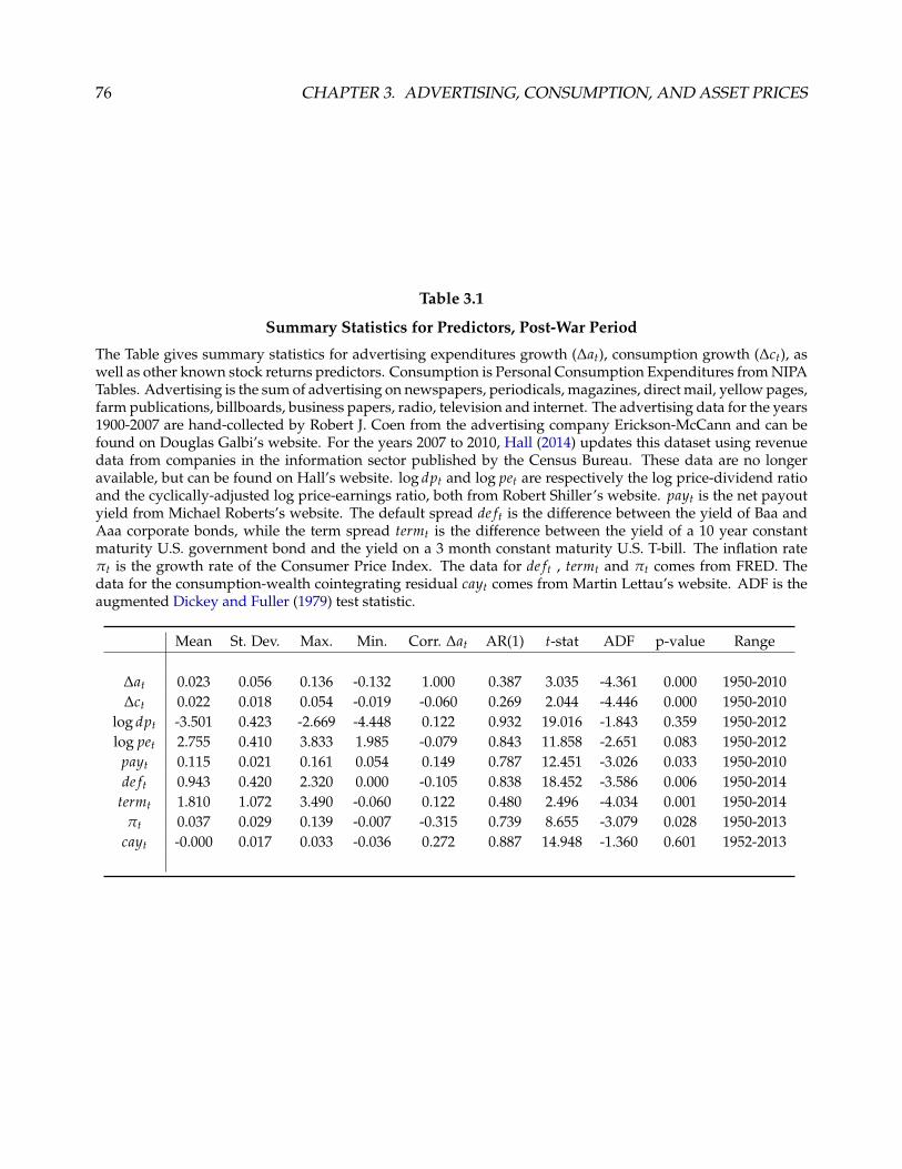
76 CHAPTER 3. ADVERTISING, CONSUMPTION, AND ASSET PRICES
Table 3.1
Summary Statistics for Predictors, Post-War Period
The Table gives summary statistics for advertising expenditures growth (∆at), consumption growth (∆ct), aswell as other known stock returns predictors. Consumption is Personal Consumption Expenditures from NIPATables. Advertising is the sum of advertising on newspapers, periodicals, magazines, direct mail, yellow pages,farm publications, billboards, business papers, radio, television and internet. The advertising data for the years1900-2007 are hand-collected by Robert J. Coen from the advertising company Erickson-McCann and can befound on Douglas Galbi’s website. For the years 2007 to 2010, Hall (2014) updates this dataset using revenuedata from companies in the information sector published by the Census Bureau. These data are no longeravailable, but can be found on Hall’s website. log dpt and log pet are respectively the log price-dividend ratioand the cyclically-adjusted log price-earnings ratio, both from Robert Shiller’s website. payt is the net payoutyield from Michael Roberts’s website. The default spread de ft is the difference between the yield of Baa andAaa corporate bonds, while the term spread termt is the difference between the yield of a 10 year constantmaturity U.S. government bond and the yield on a 3 month constant maturity U.S. T-bill. The inflation rateπt is the growth rate of the Consumer Price Index. The data for de ft , termt and πt comes from FRED. Thedata for the consumption-wealth cointegrating residual cayt comes from Martin Lettau’s website. ADF is theaugmented Dickey and Fuller (1979) test statistic.
Mean St. Dev. Max. Min. Corr. ∆at AR(1) t-stat ADF p-value Range
∆at 0.023 0.056 0.136 -0.132 1.000 0.387 3.035 -4.361 0.000 1950-2010∆ct 0.022 0.018 0.054 -0.019 -0.060 0.269 2.044 -4.446 0.000 1950-2010
log dpt -3.501 0.423 -2.669 -4.448 0.122 0.932 19.016 -1.843 0.359 1950-2012log pet 2.755 0.410 3.833 1.985 -0.079 0.843 11.858 -2.651 0.083 1950-2012
payt 0.115 0.021 0.161 0.054 0.149 0.787 12.451 -3.026 0.033 1950-2010de ft 0.943 0.420 2.320 0.000 -0.105 0.838 18.452 -3.586 0.006 1950-2014
termt 1.810 1.072 3.490 -0.060 0.122 0.480 2.496 -4.034 0.001 1950-2014πt 0.037 0.029 0.139 -0.007 -0.315 0.739 8.655 -3.079 0.028 1950-2013
cayt -0.000 0.017 0.033 -0.036 0.272 0.887 14.948 -1.360 0.601 1952-2013

3.2. AGGREGATE ADVERTISING EXPENDITURES AND EQUITY RETURNS 77
Table 3.2
Consumption Growth and Excess Returns Predictability, Post-War Period
The Table shows coefficient estimates for cumulative consumption growth (∆ct→t+τ) and excess returns (rxt→t+τ)
predictive regressions using lagged advertising expenditures growth (∆at−1→t) and consumption growth(∆ct−1→t) as predictors. Excess returns are yearly returns on the S&P 500 minus the one-year interest ratefrom Robert Shiller’s website. The t-statistics in parentheses are computed using Hansen and Hodrick (1980)standard errors. R2
adj and F are the adjusted R-squared and F-statistics, respectively.
Panel A: Consumption Growth Panel B: Excess Returns∆ct→t+1 ∆ct→t+2 ∆ct→t+3 ∆ct→t+4 rx
t→t+1 rxt→t+2 rx
t→t+3 rxt→t+4
(1) ∆at−1→t 0.129 0.160 0.128 0.085 0.293 0.476 0.956 0.910(3.25) (2.10) (1.20) (0.67) (0.78) (0.76) (1.12) (0.83)
R2adj 0.143 0.074 0.018 -0.007 -0.007 -0.005 0.015 0.001
(2) ∆ct−1→t 0.266 0.183 0.043 -0.069 -2.127 -3.291 -4.020 -6.191(2.03) (0.75) (0.14) (-0.19) (-1.92) (-1.84) (-1.74) (-2.13)
R2adj 0.051 -0.006 -0.018 -0.018 0.040 0.046 0.045 0.067
(3) ∆at−1→t 0.127 0.201 0.195 0.161 1.203 1.900 2.936 3.626(2.47) (2.00) (1.33) (0.91) (2.92) (2.88) (3.18) (2.93)
∆ct−1→t 0.010 -0.214 -0.337 -0.380 -4.404 -6.887 -9.579 -13.477(0.07) (-0.71) (-0.79) (-0.74) (-3.42) (-3.46) (-3.62) (-3.72)
R2adj 0.128 0.067 0.016 -0.010 0.128 0.148 0.215 0.224F 5.049 2.186 0.859 0.397 6.037 6.219 6.829 6.718
from one to four years. In particular, conditional on consumption growth high current advertising
growth predicts high future excess returns.
In Table 3.3, I compare the predictive power of advertising and consumption growth to the pre-
dictive power of the predictors summarized in Table 3.1. As the previous literature documents, the
dividend-price price-earnings ratios are effective at predicting long-horizon returns, while the pre-
dictive power of the payout ratio and term spread decreases with the predictive horizon. Advertising
and consumption growth, similar to cay, have high predictive power at any predictive horizon. The
term spread is the only variable that has stronger predictive power (as measured by the predictive
regression’s R-squared) than advertising and consumption at any horizon, while cay has higher pre-
dictive power at horizons of three and four years.

78 CHAPTER 3. ADVERTISING, CONSUMPTION, AND ASSET PRICES
Table 3.3
Excess Returns Predictive Regressions, Post-War Period
The Table shows coefficient estimates for cumulative excess returns (rxt→t+τ) predictive regressions using lagged
growth in advertising (∆at−1→t, conditional on lagged consumption growth ∆ct−1→t) as well as other variables,as predictors. Excess returns are yearly returns on the S&P 500 minus the one-year interest rate from RobertShiller’s website. The reported t-statistics are computed using Hansen and Hodrick (1980) standard errors.R2
adj is the adjusted R-squared statistics.
rxt→t+1 rx
t→t+2 rxt→t+3 rx
t→t+4Coeff. t-stat R2
adj Coeff. t-stat R2adj Coeff. t-stat R2
adj Coeff. t-stat R2adj
∆at−1→t 1.20 2.92 0.13 1.90 2.88 0.15 2.94 3.18 0.21 3.63 2.93 0.22∆ct−1→t -4.40 -3.42 -6.89 -3.46 -9.58 -3.62 -13.48 -3.72
log dpt−1 0.10 2.01 0.05 0.18 2.04 0.09 0.25 1.71 0.11 0.38 1.81 0.16log pet−1 -0.04 -0.86 -0.01 -0.07 -0.82 -0.00 -0.11 -0.82 0.01 -0.23 -1.15 0.04
payt−1 2.51 2.74 0.09 3.85 2.27 0.10 4.96 1.80 0.10 6.64 1.76 0.12de ft−1 0.01 0.14 -0.02 -0.04 -0.45 -0.01 -0.04 -0.31 -0.01 -0.02 -0.11 -0.02
termt−1 0.07 2.65 0.16 0.11 2.36 0.19 0.14 2.10 0.19 0.19 2.08 0.20πt−1 -0.44 -0.65 -0.01 -1.12 -0.91 0.00 -1.31 -0.69 -0.00 -0.50 -0.19 -0.02
cayt−1 2.55 2.30 0.05 5.11 2.65 0.11 8.11 2.96 0.19 11.33 3.23 0.25
In Table 3.4, I run tri-variate excess returns predictive regressions using advertising growth, con-
sumption growth and one of the other predictors as regressors, in the spirit of Huang (2015). For
every predictive horizon I consider, advertising growth (and consumption growth, omitted in the
Table) is always a significant predictor of excess stock returns. The only variables that are jointly sta-
tistically significant with advertising and consumption growth are the term spread and the payout
ratio. For horizons of two years, the default spread, inflation and cay are jointly significant. Finally,
at horizons of three and four years, cay is the only jointly significant predictor of excess returns.
3.2.2 Robustness
Table 3.5 shows the results of the estimation of a Vector-Autoregressive model of order two for ad-
vertising and consumption growth. The estimation results show that advertising growth is predicted
by consumption growth and is autocorrelated conditional on advertising growth. On the other hand,

3.2. AGGREGATE ADVERTISING EXPENDITURES AND EQUITY RETURNS 79
Table 3.4
Tri-Variate Excess Returns Predictive Regressions, Post-War Period
The Table shows coefficient estimates for cumulative excess returns (rxt→t+τ) predictive regressions using the
lagged growth in advertising (∆at−1→t) and consumption (∆ct−1→t, omitted in the Table) in tri-variate regres-sions with other predictors. Excess returns are yearly returns on the S&P 500 minus the one-year interestrate from Robert Shiller’s website. The reported t-statistics are computed using Hansen and Hodrick (1980)standard errors. R2
adj and F are the adjusted R-squared and F-statistics, respectively.
rxt→t+1 rx
t→t+2Coeff. t-stat
Coeff. t-stat R2adj F Coeff. t-stat
Coeff. t-stat R2adj F
∆at−1 ∆at−1 ∆at−1 ∆at−1
log dpt−1 1.05 2.40 0.07 1.54 0.14 4.89 1.57 2.26 0.14 1.85 0.19 4.79log pet−1 1.20 2.78 -0.00 -0.08 0.11 4.01 1.87 2.74 -0.02 -0.24 0.13 4.12
log payt−1 1.01 2.39 1.68 2.02 0.16 5.65 1.60 2.38 2.59 1.79 0.18 5.06de ft−1 1.28 3.16 -0.05 -1.23 0.13 4.54 2.11 3.47 -0.14 -2.15 0.18 6.69
termt−1 1.48 2.47 0.05 1.94 0.27 4.57 1.49 1.53 0.08 1.88 0.22 2.76πt−1 1.21 3.07 -0.93 -1.68 0.16 5.67 1.87 3.06 -2.00 -2.13 0.21 6.88
cayt−1 1.01 2.26 1.83 1.74 0.16 6.11 1.45 2.15 4.06 2.36 0.23 7.29
rxt→t+3 rx
t→t+4Coeff. t-stat
Coeff. t-stat R2adj F
Coeff. t-statCoeff. t-stat R2
adj F∆at−1 ∆at−1 ∆at−1 ∆at−1
log dpt−1 2.54 2.74 0.17 1.47 0.25 4.71 2.91 2.32 0.26 1.57 0.29 4.60log pet−1 2.88 3.13 -0.03 -0.29 0.20 4.48 3.43 2.81 -0.08 -0.52 0.22 4.41
log payt−1 2.61 2.83 2.87 1.31 0.24 4.85 3.10 2.52 4.34 1.44 0.26 4.85de ft−1 3.20 3.68 -0.17 -1.78 0.25 6.37 3.82 3.24 -0.17 -1.16 0.24 5.36
termt−1 2.18 1.63 0.10 1.57 0.25 2.50 2.83 1.81 0.15 1.70 0.32 3.43πt−1 2.89 3.34 -2.26 -1.65 0.26 6.47 3.85 3.63 -2.82 -1.61 0.33 8.33
cayt−1 2.17 2.50 5.92 2.63 0.31 7.71 2.58 2.60 7.91 2.97 0.38 10.04

80 CHAPTER 3. ADVERTISING, CONSUMPTION, AND ASSET PRICES
Table 3.5
VAR Model for Advertising and Consumption Growth, Post-War Period
The Table shows coefficient estimates for a Vector-Autoregressive (VAR) model of advertising expenses andconsumption growth (∆a and ∆c, respectively). The t-statistics are in parentheses. In each equation, R2 and Fare the R-squared and F-statistics, respectively.
Panel A: One Lag Panel B: Two Lags∆at→t+1 ∆ct→t+1 ∆at→t+1 ∆ct→t+1
∆at−1→t 0.679 0.127 0.515 0.124(4.71) (2.52) (3.23) (2.16)
∆at−2→t−1 0.242 -0.0167(1.49) (-0.28)
∆ct−1→t -1.417 0.0105 -1.119 0.0681(-3.11) (0.07) (-2.39) (0.41)
∆ct−2→t−1 -1.180 0.00771(-2.38) (0.04)
R2 0.274 0.158 0.336 0.170F 11.12 5.521 7.333 2.973
consumption growth is not conditionally autocorrelated and is predicted by advertising expenditu-
res growth.
Table 3.6 shows the results of Table 3.5 for different sub-samples of my dataset. In Panel A, I re-
port the results for the 1922-2009 sample, while in Panel B for the 1982-2009 sample.5 The results
show that the dynamics of the advertising-consumption relationship dynamic dramatically change
over the course of the last century. The sign of the VAR coefficients does not change across diffe-
rent samples, but their magnitude and statistical significance increases when I restrict the sample to
more recent years. The time-varying relation between advertising growth and consumption growth
therefore limits the use of advertising growth as an instrumental variable for expected consumption
growth, and rathers calls for a model to explore the joint dynamics of the variables.
5Tests for cointegration between consumption and advertising in these two samples fail to reject the null hypothesis ofno cointegration.

3.2. AGGREGATE ADVERTISING EXPENDITURES AND EQUITY RETURNS 81
Table 3.6
VAR Model for Advertising and Consumption Growth, 1922-2009 and 1982-2009
The Table shows coefficient estimates for a Vector-Autoregressive (VAR) model of advertising expenses andconsumption growth (∆a and ∆c, respectively) across different samples. The t-statistics are in parentheses. Ineach equation, R2 and F are the R-squared and F-statistics, respectively.
Panel A: 1922-2009 Panel B: 1982-2009One Lag Two Lags One Lag Two Lags
∆at→t+1 ∆ct→t+1 ∆at→t+1 ∆ct→t+1 ∆at→t+1 ∆ct→t+1 ∆at→t+1 ∆ct→t+1
∆at−1→t 0.352 0.0666 0.301 0.0433 0.783 0.166 0.454 0.117(2.97) (1.16) (2.39) (0.70) (4.10) (3.37) (2.73) (2.25)
∆at−2→t−1 0.0602 0.0572 0.856 0.137(0.49) (0.95) (4.53) (2.31)
∆ct−1→t -0.242 0.140 -0.190 0.159 -1.312 0.224 -1.614 0.155(-0.95) (1.13) (-0.73) (1.25) (-1.95) (1.29) (-2.36) (0.72)
∆ct−2→t−1 -0.124 -0.0885 -1.900 -0.261(-0.47) (-0.70) (-3.15) (-1.38)
R2 0.0966 0.0612 0.0825 0.0676 0.383 0.543 0.651 0.604F 4.759 2.900 1.978 1.596 8.992 17.24 13.06 10.70

82 CHAPTER 3. ADVERTISING, CONSUMPTION, AND ASSET PRICES
Table 3.7
Consumption Growth Predictive Regressions, Post-War Period
The Table shows coefficient estimates for cumulative consumption growth (∆ct→t+τ) predictive regressionsusing lagged consumption growth (∆ct−1→t), advertising expenditures growth (∆at−1→t), as well as the laggedshort-term interest rate (r3m
t−1) and lagged term spread from t− 1 to t− 1 + τ (rτt−1 ) (Harvey (1988)) as predictors.
The short-term interest rate is the yield on a 3 month constant maturity U.S. T-bill, and the term spread is thedifference between a U.S. government bond with constant maturity τ and the short-term interest rate. The datais from FRED. The t-statistics in parentheses are computed using Hansen and Hodrick (1980) standard errors.R2
adj and F are the adjusted R-squared and F-statistics, respectively.
∆ct→t+1 ∆ct→t+2 ∆ct→t+3 ∆ct→t+4
(1) r3mt−1 0.001 0.001 0.003 0.071
(0.85) (0.26) (0.81) (0.70)rτ
t−1 0.020 0.030 0.023 0.063(1.82) (2.81) (1.80) (0.65)
R2adj 0.172 0.272 0.146 0.072F 2.590 3.669 1.588 0.654
(2) ∆at−1→t 0.149 0.395 0.541 0.629(2.36) (3.51) (3.07) (3.25)
∆ct−1→t 0.241 -0.281 -0.786 -1.104(1.21) (-0.76) (-1.38) (-1.65)
r3mt−1 -0.000 -0.002 -0.001 0.023
(-0.38) (-1.17) (-0.43) (0.29)rτ
t−1 0.010 0.013 0.009 0.022(1.14) (1.59) (0.87) (0.29)
R2adj 0.475 0.519 0.351 0.305F 7.511 6.196 3.154 2.599
In Table 3.7, I test the robustness of advertising growth in predicting consumption growth, by aug-
menting specification (3) of Table 3.2 with an additional predictor. To the best of my knowledge, the
term structure of the interest rates is one of the few variables known to predict consumption growth
at long horizons. I follow Harvey (1988) and run consumption growth predictive regressions using
the short-term risk-free rate and the term spread as a proxy for the term structure. Specification (1)
of Table 3.7 confirms that the term structure is a good predictor of consumption growth at horizons
from one to three years. Specification (2) shows that the predictive power of advertising growth
significantly decreases the predictive power of the term structure at any predictive horizon.

3.3. MODEL 83
Figures 3.4 and Table 3.8 report the results of my third robustness test, which measures the out-of-
sample performance of advertising growth in predicting excess returns using both moving-window
and expanding-window regressions. In moving-window regressions, I use a fixed rolling window of
fifty observations as fitting sample. In expanding-window regressions, I start with fitting the model
on the first fifty annual observations, and expand the sample one observation at a time to obtain the
full 1950-2010 sample. Figure 3.4 plots point estimates for the coefficients of one-year-ahead excess
returns predictive regressions, as well as their associated 95 percent confidence intervals, for the out-
of-sample period 1980-2010. In both moving regressions (Panel A) and expanding regressions (Panel
B), the regression coefficient associated to advertising growth is around one (but for years 2003-2008
in moving regressions), and always statistically different from zero at a 95 percent confidence level.
Finally, Table 3.8 reports the results of the out-of-sample R-squared statistics of Campbell and Thomp-
son (2008) and the adjusted mean squared prediction error (MSPE) statistics of Clark and West (2007).
The out-of-sample R-squared displays similar values in moving and expanding regressions. The
within-sample R-squared increases with the predictive horizon. The adjusted-MSPE statistics speaks
in favor of long-run predictability. The (one-sided) t-statistic for a difference in predictive accuracy
between within sample and out-of-sample predictions is rejected in both moving and expanding
regressions at a five percent confidence level for horizons of two to four years.
Finally, in Appendix C.2 I show that advertising growth predicts a component of aggregate con-
sumption growth not captured by the Bansal and Yaron (2004) long-run risk. In the next Section, I
introduce a dynamic investment-based asset pricing model of frictions in the goods market to repli-
cate the observed predictive power of advertising expenditures on aggregate consumption growth
and excess returns.
3.3 Model
The model is a discrete-time, dynamic stochastic general equilibrium model with two goods. The
economy is populated by a continuum of identical households and a continuum of identical firms.
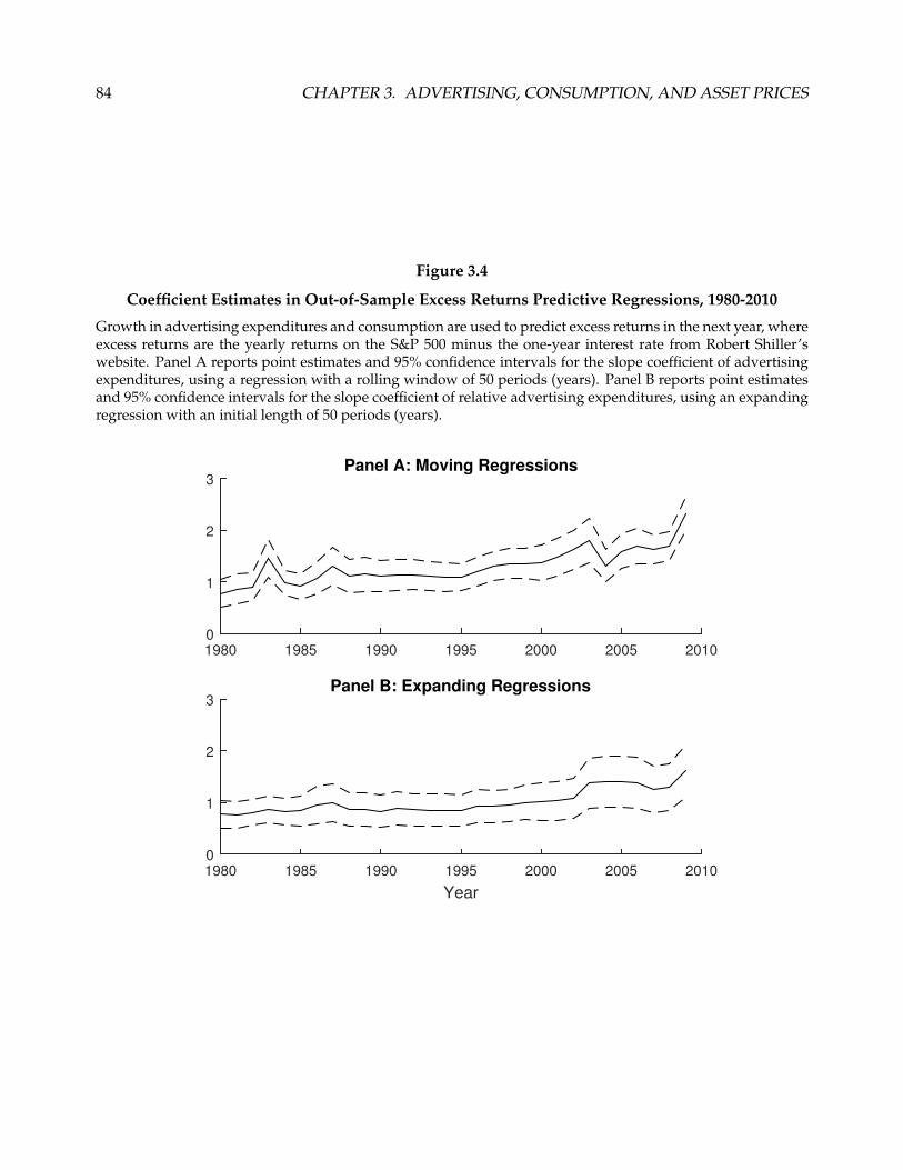
84 CHAPTER 3. ADVERTISING, CONSUMPTION, AND ASSET PRICES
Figure 3.4
Coefficient Estimates in Out-of-Sample Excess Returns Predictive Regressions, 1980-2010
Growth in advertising expenditures and consumption are used to predict excess returns in the next year, whereexcess returns are the yearly returns on the S&P 500 minus the one-year interest rate from Robert Shiller’swebsite. Panel A reports point estimates and 95% confidence intervals for the slope coefficient of advertisingexpenditures, using a regression with a rolling window of 50 periods (years). Panel B reports point estimatesand 95% confidence intervals for the slope coefficient of relative advertising expenditures, using an expandingregression with an initial length of 50 periods (years).
1980 1985 1990 1995 2000 2005 20100
1
2
3Panel A: Moving Regressions
Year1980 1985 1990 1995 2000 2005 20100
1
2
3Panel B: Expanding Regressions

3.3. MODEL 85
Table 3.8
Out-of-Sample Excess Returns Predictive Regressions
The Table shows the out-of-sample performance of cumulative excess returns (rxt→t+τ) predictive regressions
using lagged growth in advertising (∆at−1→t) and consumption (∆ct−1→t) as predictors. The statistic R2ws is the
within-sample adjusted R-squared statistic. Out-of-sample moving regressions use a 30-year rolling windowto predict cumulative excess returns at different horizons, starting from 1980. Out-of-sample expanding regres-sions use the initial 1950-1980 sample to predict cumulative excess returns at different horizons. The procedureis then repeated by expanding the sample in one-year steps until the full 1950-2010 sample is obtained. Thestatistic R2
osis the out-of-sample R-squaredd statistic detailed in Campbell and Thompson (2008). The Newey-West (NW) t-statistics are obtained from regressing the adjusted-MSPE statistics of Clark and West (2007) on aconstant. The test is a one-side test for a zero coefficient.
Within-Sample Out-of-Sample Moving Out-of-Sample ExpandingHorizon (years) R2
ws R2os NW t-stat. R2
os NW t-stat.
1 0.128 0.071 1.216 0.066 1.3852 0.148 0.129 1.916 0.114 2.0173 0.215 0.153 2.005 0.147 2.4194 0.224 0.139 2.349 0.177 3.178
The model features two key frictions. First, absent advertising households in the economy are only
aware of the existence of their endowment (numeraire) good. Firms overcome this friction by spen-
ding resources to advertise their product. Once firms and customers match with each other, they
form a relationship that lasts for multiple periods. Second, the advertising process is subject to se-
arch externalities. Times when all the firms in the economy post many advertisements are also times
when it is harder for an individual firm to attract a customer by posting an advertisement (ad). In
particular, once every firm has posted its ad’s, the sum of the individual ad’s in the economy de-
termines the probability that one ad will turn into a customer for an individual firm.6 I denote this
probability by λ. I assume that product search is costless for the household, and normalize the hou-
sehold search cost to one. Using a den Haan et al. (2000) function with elasticity ϑ > 0, the matching
function between a household and an ad is given by
G (ad) =ad(
1 + adϑ)1/ϑ
. (3.1)
6For tractability, I abstract from the difference between customer and marketing/brand capital (Drozd and Nosal(2012)), where advertising expenditures build marketing capital, which in turn determines the likelihood of attractingnew customers.

86 CHAPTER 3. ADVERTISING, CONSUMPTION, AND ASSET PRICES
Denoting aggregate variables with uppercase letters, the probability λ that an advertisement attracts
a household is a function of the total ad’s in the economy:
λ (AD) =G (AD)
AD=
1(1 + ADϑ
)1/ϑ. (3.2)
Finally, customer relations are long-lasting. I denote the stock of firm customers (customer capital,
Gourio and Rudanko (2014)) by n and assume that in each period t the firm loses an exogenous
fraction ϕ ∈ [0, 1] of its customers. The aggregate law of motion for customer capital between period
t and period t + 1 is then
Nt+1 = (1− ϕ) Nt + G (ADt) (3.3)
= (1− ϕ) Nt + λ (ADt) ADt. (3.4)
3.3.1 Firm Problem and Return on Equity
Firms enter each time period with a stock of customers, observe the aggregate endowment of the
numeraire good and decide how much to spend in advertising to build their customer capital. Firm
revenue is the product between the unit price of the manufactured good and the number of firm
customers. Moreover, firms pay a convex advertising cost to attract customers. Three assumptions
on firm profits allow to simplify the analysis while retaining the model’s main insights. First, firms
extract all the matching surplus from households, so that the manufactured good’s price is the mar-
ginal rate of intratemporal substitution between the manufactured good and the numeraire. This
eliminates the issue of time-inconsistent pricing (Nakamura and Steinsson (2011)). Second, I do not
explicitly model production of the advertised good. I assume that the advertised good is always
available for firms to buy and re-sell to households at the price of purchase once a firm finds a custo-
mer. This allows to reduce the state space and focus on the implications of advertising externalities
for return predictability. Finally, the model features convex advertising costs to reduce the volatility
of advertising.
As in Liu et al. (2009) and Kuehn et al. (2012), the firm’s problem at time t is to maximize the discoun-
ted expected value of its dividend stream St, subject to the law of motion for its customer base and

3.3. MODEL 87
a non-negativity constraint on advertising. Let Pt denote the period-t relative price of the advertised
good in terms of the numeraire. The representative firm’s problem is
St = max{ADt+j}∞
j=0
Et
∞
∑j=0
Mt+j
Pt+j −χ
2
(ADt+j
Nt+j
)2Nt+j, (3.5)
subject to, for all j,
ADt+j ≥ 0 (3.6)
and the law of motion (3.3). Here, Mt+j denotes the stochastic discount factor (SDF) between t and
t + j, χ is a convex adjustment cost parameter and (3.6) is a non-negativity constraint on effort. Since
the matching probability λt is greater than zero, (3.6) can be re-written as
λt+j ADt+j ≥ 0. (3.7)
Substituting the first constraint into (3.5), and respectively denoting by µnt and µλ
t the time-t Lagrange
multipliers on (3.3) and (3.7), the problem’s first order conditions are
µnt =
χ
λt
ADt
Nt− µλ
t , (3.8)
µnt = Et Mt+1
[Pt+1 +
χ
2
(ADt+1
Nt+1
)2+ (1− ϕ) µn
t+1
], (3.9)
plus the Kuhn-Tucker conditions on (3.3) and (3.7). The Euler equation for customer capital accumu-
lation is therefore
χ
λt
ADt
Nt− µn
t = Et Mt+1
[Pt+1 +
χ
2
(ADt+1
Nt+1
)2+ (1− ϕ)
(χ
λt+1
ADt+1
Nt+1− µn
t+1
)]. (3.10)
The Euler equation relates the marginal cost of adding one unit of search effort at time t to the mar-
ginal benefit in period t + 1 of having λt additional customers, in turn consisting of higher revenues,
lower adjustment costs, higher servicing costs and the discounted marginal cost of postponing to

88 CHAPTER 3. ADVERTISING, CONSUMPTION, AND ASSET PRICES
period t + 1 the unit increase in advertising. Note that at the optimum
St = Et
∞
∑j=0
Mt+j
[Pt+jNt+j −
χ
2
AD2t+j
Nt+j− κNt+j (3.11)
+ µnt+j((1− ϕ) Nt+j + λt+j ADt+j − Nt+j+1
)+ µλ
t+jλt+j ADt+j
],
so that expanding St, I get
St = PtNt −χ
2AD2
tNt− κNt + µn
t ((1− ϕ) Nt + λt ADt − Nt+1) + µλt λt ADt
+ Et Mt+1
[Pt+1Nt+1 −
χ
2AD2
t+1Nt+1
− κNt+1 (3.12)
+ µnt ((1− ϕ) Nt+1 + λt+1ADt+1 − Nt+2) + µλ
t+1λt+1ADt+1 + . . .]
. (3.13)
Recursively substituting (3.10) into (3.12) the equilibrium, cum-dividend price of equity is
St =
(Pt +
χ
2
(ADt
Nt
)2+ (1− ϕ) µn
t
)Nt, (3.14)
and the ex-dividend stock price denoted by St is equal to
St = µnt Nt+1. (3.15)
Finally note that whenever (3.6) does not bind at time t (i.e., advertising is positive) the return of one
unit of advertising is equal to the return on equity Rt+1 between t and t + 1, and is given by
Rt+1 =St+1
St(3.16)
=1
µnt
(Pt+1 +
χ
2
(ADt+1
Nt+1
)2+ (1− ϕ) µn
t+1
)(3.17)
The return on equity, as in Cochrane (1991), is the trade-off between the marginal benefit of posting
an additional ad in period t - accrued between period t and t + 1 - and the ad cost incurred in period
t. Note that for a given level of past advertising, high current advertising and therefore high cur-
rent advertising growth reduce future expected returns. This happens because i) through the goods
market friction high advertising reduces the probability that an additional ad will turn into a custo-

3.3. MODEL 89
mer (from (3.8), µn is decreasing in λ) and ii) high current advertising (and future customer capital)
reduces future marginal revenues.
3.3.2 Household Problem
The household derives its period utility from a bundle of the numeraire good and the advertised
good, and decides how much of its endowment to allocate to consumption, investment in a claim to
firm profits and investment in a risk-free bond. Denote by C0 and C1 the representative household’s
consumption of the numeraire and advertised goods, respectively. Further denote by Y the endo-
wment of the numeraire good, by φ the household investment in claims to the firm profits, and by
θ the household investment in a risk-free asset with current price of one and gross return R f . The
claims to firm profits and the risk-free assets are in unit and zero aggregate net supply, respectively.
The household’s budget constraint at time t + j is therefore
C0,t+j ≤ Yt+j + φt+j−1St+j + θt+j−1R ft+j − Pt+jC1,t+j − φt+jSt+j − θt+j. (3.18)
Moreover, I assume that each firm customer consumes only one unit of the advertised good, so that
C1,t+j ≤ Nt+j. The household’s intraperiod utility is given by the CES function
u (C0; C1) =
((1− α)C
η−1η
0 + αCη−1
η
1
) ηη−1
, (3.19)
where α ∈ [0, 1], and η ≥ 0 is the elasticity of substitution between the numeraire and manufactu-
red goods. Finally, the household’s intertemporal utility is denoted by Vt, and is specified by the
recursion
Vt =
{(1− β) u (C0,t; C1,t)
1− 1ψ + βEt
[V1−γ
t+1
] 1−1/ψ1−γ
} 11−1/ψ
, (3.20)
where β is the time discount factor, ψ is the elasticity of intertemporal substitution, and γ is the
relative risk aversion coefficient (Kreps and Porteus (1978), Epstein and Zin (1989)). The relative

90 CHAPTER 3. ADVERTISING, CONSUMPTION, AND ASSET PRICES
price of C1 is the marginal rate of substitution between C0 and C1, or
P =α
1− α
(C1
C0
)− 1η
. (3.21)
In Appendix C.3 I show that the stochastic discount factor is
Mt+1 = β
(C0,t+1
C0,t
)− 1η(
u (C0,t+1; C1,t+1)
u (C0,t; C1,t)
) 1η−
1ψ
Vt+1
Et
(V1−γ
t+1
) 11−γ
1ψ−γ
. (3.22)
Note that, for a fixed level of past advertising, high current advertising and therefore high current
advertising growth increase customer capital, decrease the numeraire good’s consumption, and in-
crease the stochastic discount factor. This and the fact that future expected returns (3.16) are decrea-
sing in advertising growth implies that high advertising growth generates high negative co-variation
between the stochastic discount factor and expected excess returns, and therefore high risk premia.
Finally, the risk-free rate is
R ft+1 =
1Et [Mt+1]
. (3.23)
3.3.3 Equilibrium
For each combination of the state variables (Y; N), a competitive equilibrium of search in the goods
market specifies policy functions for firm advertising AD (Y; N); policy functions for household
numeraire consumption C0 (Y; N), stock holdings φ (Y; N) and risk-free asset holdings θ (Y; N); a
stock price S (Y; N), a risk-free rate R f (Y; N) and a relative price of the manufactured good in terms
of the numeraire P (Y; N), such that firms and households maximize their constrained objectives,
markets for the numeraire and the advertised goods clear, and aggregate stock and bond markets
clear. In particular, note that the equilibrium conditions in the goods market imply that
C0 = Y− χ
2
(ADN
)2N, (3.24)
and C1 = N.

3.4. RESULTS 91
3.4 Results
Section 3.4.1 describes my calibration strategy and solution method. Section 3.4.2 compares the pre-
dictability results coming from simulations of the model to those coming from post-war US data.
Finally, section 3.4.3 highlights the quantitative importance of goods market frictions in obtaining
the predictability results.
3.4.1 Calibration and Computation
I calibrate the model at an annual frequency. In my calibration strategy I do not try to match the
equity returns predictive regression coefficients found in the data, but rather show that the sign,
magnitude and statistical significance of these coefficients arise naturally when the model is calibra-
ted to match other data moments. Broda and Weinstein (2010) report a median annualized entry
rate of new goods in consumer baskets equal to 0.25. When normalizing household search effort to
unit, this entry rate in the model is equal to(1 + AD−ϑ
)−1/ϑ, which I target to a steady-state value of
0.30 with a matching function elasticity ϑ = 0.57. Finally, the results are not sensitive to the convex
adjustment cost parameter χ, which I therefore set equal to one. On the household side, Petrosky-
Nadeau and Wasmer (2015) document that average annual expenditures on food consumed at home,
plus utilities, amount to 10-15 percent of total annual expenditures in the 1984-2009 Household Con-
sumption Expenditure Survey. I target this share in the model to 17 percent with a bias parameter α
equal to 0.79. I use an AR(1) process in logs to describe the time-series evolution of the numeraire
good’s endowment, and set the persistence and volatility of the endowment process equal to 0.75
and 0.13, respectively. Finally, I set the relative risk aversion coefficient γ equal to 21. The last three
parameters target a equity premium of three percent, a equity premium volatility of twelve percent
and a consumption growth volatility of 1.8 percent while retaining the main predictability results.
I borrow the remaining parameters from the literature. I choose a customer capital depreciation
rate ϕ equal to 0.20 as in Gourio and Rudanko (2014), in the mid-range of the empirical estimates
of Bronnenberg et al. (2012) and in the low range of the estimates of Broda and Weinstein (2010).

92 CHAPTER 3. ADVERTISING, CONSUMPTION, AND ASSET PRICES
Modeling household preferences, I set the annual discount rate β to 0.95, and the intertemporal
elasticity of substitution ψ to 1.5 following Bansal and Yaron (2004). Finally, I set the elasticity of
substitution parameter η equal to 0.83 following the international trade literature (Heathcote and
Perri (2002), Bianchi (2009) and Huo and Rıos-Rull (2013)).
The model is challenging to solve numerically. First, the equilibrium allocations are not Pareto-
optimal. A social planner confronted with the constrained equity maximization problem (3.5) would
in fact internalize the congestion effect created by search effort, while individual firms do not. This in
turn requires solving the model using its first-order conditions. Second, the non-negativity constraint
on search effort renders perturbation methods not suited for this type of problems. For these reasons,
I solve for the competitive search equilibrium using the globally nonlinear computational algorithm
of Petrosky-Nadeau and Zhang (2017). In particular, for each point in the aggregate endowment-
customer capital state space (Yt, Nt), the algorithm solves for optimal advertising AD∗t = AD (Yt, Nt)
and the multiplier on its non-negativity constraint µn∗t = µn (Yt, Nt) from the Euler equation
χ
λt
ADt
Nt− µn (Yt, Nt) = Et Mt+1
[Pt+1 + (1− ϕ)
(χ
λt+1− µn (Yt, Nt)
)], (3.25)
where both λt and Pt are functions of AD (Yt, Nt). Appendix C.4 provides details on the computati-
onal algorithm.
3.4.2 Simulated Moments and Predictability
I simulate ten thousand samples of sixty-one annual observations, and in each simulated sample
compute average advertising and consumption growth, return on equity and risk-free rate. Mo-
reover, in each simulated sample I run predictive regressions of equity returns using consumption
growth and advertising growth as predictors.
Panel A of Table 3.9 reports the average first moment and standard deviation of advertising and con-
sumption growth, equity premium and risk-free rate across the simulated samples. Panel B reports
the corresponding moments in post-war US data. The calibration of the model allows to reasonably

3.4. RESULTS 93
Table 3.9
Model-Simulated Moments
Panel A: Model Panel B: DataMean St. Dev Mean St. Dev
∆a 0.026 0.237 0.023 0.056∆c 0.001 0.021 0.022 0.018
R− R f 0.052 0.173 0.066 0.164R f 0.003 0.056 0.017 0.027
match the first moments of the selected variables, and to match the volatility of consumption growth,
equity premium and risk-free rate.
Table 3.10 tests the predictive power of advertising and consumption growth on future equity re-
turns. As in the data, neither advertising nor consumption growth can alone predict future returns
in the model. Moreover, Conditional on consumption growth, advertising growth however signi-
ficantly predicts future returns. The predictive power of advertising (and consumption) is higher
at longer horizons, and the economic magnitude of the coefficients is close their empirical counter-
parts. As in the data, advertising positively predicts consumption growth and is therefore a priced
aggregate risk factor. Through customer capital, in fact, advertising growth determines growth in
consumption of the manufactured good and increases the numeraire goods’ future marginal utility.
At the same time, advertising growth reduces expected returns to investing in claims to customer
capital. These conditions imply that times when firms spend more resources in advertising are times
of low expected returns and high expected marginal utility, and therefore high risk premia.
3.4.3 The Quantitative Impact of Goods Market Frictions
In this section, I use the insights of the model to explore the effect of goods market frictions on
predictability. In particular, I show that the congestion effect created by aggregate advertising is
quantitatively important in driving both consumption and returns predictability.

94 CHAPTER 3. ADVERTISING, CONSUMPTION, AND ASSET PRICES
Table 3.10
Results: Returns Predictability
The Table shows coefficient estimates for cumulative returns (rt→t+τ) predictive regressions coming from mo-del simulations (Panel A) and from post-war data (Panel B) using lagged advertising expenditures growth(∆at−1→t) and consumption growth (∆ct−1→t) as predictors. The t-statistics in parentheses are computed usingHansen and Hodrick (1980) standard errors.
Panel A: Model Panel B: Data (Post-War)rt→t+1 rt→t+2 rt→t+3 rt→t+4 rt→t+1 rt→t+2 rt→t+3 rt→t+4
(1) ∆at−1→t -0.084 -0.144 -0.219 -0.263 0.358 0.636 1.273 1.385(-0.67) (-1.33) (-1.65) (-1.67) (0.94) (0.96) (1.38) (1.13)
R2adj 0.027 0.030 0.037 0.038 -0.003 0.003 0.031 0.016
(2) ∆ct−1→t -0.103 -0.179 -0.270 -0.326 -2.189 -3.410 -4.121 -6.843(-1.11) (-1.42) (-1.74) (-1.75) (-1.94) (-1.81) (-1.64) (-2.12)
R2adj 0.028 0.032 0.040 0.041 0.042 0.045 0.038 0.065
(3) ∆at−1→t 4.334 8.512 12.198 15.543 1.332 2.204 3.492 4.644(1.83) (1.92) (2.13) (2.20) (3.24) (3.24) (3.57) (3.51)
∆ct−1→t -5.071 -9.934 -14.242 -18.126 -4.712 -7.583 -10.731 -16.174(-1.46) (-1.95) (-2.16) (-2.23) (-3.66) (-3.69) (-3.82) (-4.16)
R2adj 0.069 0.103 0.132 0.149 0.150 0.175 0.246 0.277

3.4. RESULTS 95
Figure 3.5
Customer Capital Investment
The Figure compares the optimal customer capital investment λE in the decentralized economy with the in-vestment in the decentralized economy. Panel A shows the investment as a function of customer capital N,for the lowest possible realization of the endowment process Y. Panel B shows the investment as a function ofcustomer capital N, for the highest possible realization of the endowment process Y.
0.5 1 1.5 2 2.5 3 3.5 40.1
0.2
0.3
0.4Panel A: Low Endowment
DecentralizedCentralized
Customers0.5 1 1.5 2 2.5 3 3.5 4
0.1
0.2
0.3
0.4
0.5Panel B: High Endowment
DecentralizedCentralized
As noted before, the equilibrium allocation in the decentralized economy is not Pareto-optimal. To
solve for the Pareto-optimal allocation, I keep the same steady-state parametrization of the model
described in section 3.4.1 and solve the constrained optimization problem (3.5) using standard value
function iteration. Since firms in the centralized economy do not over-advertise to compensate the
congestion effect created by aggregate advertising, the optimal amount of firm search effort in the
centralized economy is as much as ten times lower than in the decentralized economy. Figure 3.5
shows that as a consequence the effective firm investment in customer capital, λE, is low and almost
flat.
Table 3.11 reports estimates of the same predictive regressions coefficients of Tables (??) and (3.10)

96 CHAPTER 3. ADVERTISING, CONSUMPTION, AND ASSET PRICES
Table 3.11
Predictability in the Centralized Economy
The Table shows coefficient estimates for cumulative consumption growth (∆ct→t+τ) and returns (rt→t+τ) pre-dictive regressions coming from simulations of the centralized economy, using lagged advertising expendi-tures growth (∆at−1→t) and consumption growth (∆ct−1→t) as predictors. The t-statistics in parentheses arecomputed using Hansen and Hodrick (1980) standard errors.
Panel A: Consumption Panel B: Returns∆ct→t+1 ∆ct→t+2 ∆ct→t+3 ∆ct→t+4 rt→t+1 rt→t+2 rt→t+3 rt→t+4
(1) ∆at−1→t -0.116 -0.228 -0.325 -0.378 -0.121 -0.213 -0.326 -0.403(-1.00) (-1.51) (-1.86) (-1.90) (-1.10) (-1.41) (-1.64) (-1.82)
R2adj 0.024 0.033 0.042 0.043 0.024 0.027 0.035 0.039
(2) ∆ct−1→t -0.100 -0.197 -0.278 -0.327 -0.103 -0.184 -0.282 -0.350(-1.00) (-1.80) (-1.89) (-2.00) (-1.04) (-1.30) (-1.74) (-1.92)
R2adj 0.025 0.035 0.045 0.048 0.025 0.030 0.038 0.042
(3) ∆at−1→t 0.159 0.343 0.385 0.552 0.113 0.293 0.398 0.597(0.24) (0.42) (0.53) (0.44) (0.15) (0.32) (0.45) (0.43)
∆ct−1→t -0.219 -0.463 -0.581 -0.765 -0.186 -0.405 -0.588 -0.820(-0.40) (-0.84) (-0.87) (-0.84) (-0.32) (-0.54) (-0.69) (-0.89)
R2adj 0.041 0.047 0.054 0.058 0.041 0.041 0.050 0.054
for the centralized economy. The results show that the volatility of advertising in the decentralized
economy has key implications for predictability. On the consumption predictability side companies
do not over-advertise in the centralized economy, customer capital growth is flat and current ad-
vertising growth does not generate large movements in future customer capital and consumption.
On the returns predictability side, a flat effective investment in customer capital (λE) reduces the
large shifts in marginal profits and marginal utility due to over-advertising, thus reducing the risk
associated with advertising and the predictive power of advertising on future returns.
3.5 Conclusion
In this paper, I provide new evidence on the importance of advertising and goods market frictions
for financial economics. I show that advertising growth predicts future consumption growth in post-

3.5. CONCLUSION 97
war US data, and use this result to verify the core prediction of dynamic asset pricing theory that
expected consumption matters for expected returns. Using advertising and consumption growth to
predict excess returns on equity I show that advertising positively predicts excess returns at horizons
of up to four years. Motivated by these empirical findings, I build a general equilibrium model of
frictional goods markets where advertising is an investment in long-lasting customer relationships
that affect the dynamics of household consumption. The calibrated model is able to replicate the
predictive power of advertising growth on future consumption growth and equity returns observed
in the data, and highlights the importance of frictions in the goods market to quantitatively match
these predictability patterns.
The paper is part of a small literature in financial economics highlighting the importance of adverti-
sing and goods market frictions at the firm level (Gourio and Rudanko (2014), Vitorino (2014)). In this
paper, I show that goods market frictions are also quantitatively relevant in the aggregate. As such,
future research should be devoted to further studying the aggregate implications (i.e. the trade-off
between customer capital and other forms of tangible and intangible capital) and the welfare impact
of these frictions.

98 CHAPTER 3. ADVERTISING, CONSUMPTION, AND ASSET PRICES

Appendix A
Appendix to Chapter 1
99

100 APPENDIX A. APPENDIX TO CHAPTER 1
A.1 Solving for the Optimal Contract
Substituting the manager’s first incentive-compatibility (1.5) constraint into (1.2)-(1.4), the problem
becomes finding m (y) and π1 (y) to maximize
L =∫ y
¯y[P−m (y) (P− π1 (y) + k)] dF (y)− I + ω
∫ y
¯y[y− P + m (y) (P− π1 (y))] dF (y)
+∫ y
¯y[µ (y) [y− P + m (y) (P− π1 (y))] + λ (y) [P−m (y)π1 (y)]] dy, (A.1)
where ω, µ (y), and λ (y) respectively denote the multipliers on (1.3), (1.4), and (1.6). Taking first-
order conditions of (A.1) with respect to m (y) yields
∂L∂m (y)
= [P− π1 (y)] [(ω− 1) f (y) + µ (y)]− k f (y)− λ (y)π1 (y) . (A.2)
If m (y) = 1, it must be that ∂L/∂m (y) > 0.A.1 Therefore,
[P− π1 (y)] [(ω− 1) f (y) + µ (y)] > k f (y) + λ (y)π1 (y) ≥ 0. (A.3)
This implies that R− π1(y) > 0 and λ∗ (y) = 0. On the other hand,
∂L∂π1 (y)
= f (y) (1−ω)− µ (y) , (A.4)
implying that to satisfy ∂L/∂π1 (y) ≥ 0, ω∗ ≤ 1. Then from (A.3), µ (y) > 0 and the limited-liability
constraint must bind such that in the monitoring region π1 (y) = y.
A.1For a given y, if m (y) = 1 it must be that (L (m (y) = 1)−L (m (y) = 0)) /(1− 0) > 0.

A.2. ADDITIONAL RESULTS: BANK VALUE 101
A.2 Additional Results: Bank Value
Table A1
Robustness and Placebo Tests: Market-to-Book
This table reports sample bandwidth selection tests (Panel A) and placebo tests (Panel B) on my main Market-to-Book result. In the first four specifications of Panel A, I use two small samples of BHCs with average 2005total assets between $400 and $600 million (Specifications (1) and (2)), and between $300 and $700 million(Specifications (3) and (4)). In the last four specifications I use two large samples of BHCs with total assetsbetween $150 million and $1 billion (Specifications (5) and (6)), and between $150 million and $1.5 billion(Specifications (7) and (8)). In the first six specifications of Panel B, I use asset thresholds of $300 million, $750million and $1 billion to separate treated and control BHCs. In Specifications (7) and (8) I use the last quarterof 2004 as treatment quarter, dropping post-2005 observations from the sample. In the last two specifications,I use the last quarter of 2006 as treatment quarter. The dependent variable in all specifications is the naturallogarithm of Tobin’s q. Unreported control variables include leverage, Tier 1 Ratio, total assets, profitability,ROE, diversification, and asset growth.
Panel A: Sample Bandwidth Selection
$400M-600M $300M-700M $150M-1B $150M-1.5B
(1) (2) (3) (4) (5) (6) (7) (8)
Post × Treated -0.087** -0.088** -0.055** -0.072*** -0.052** -0.073*** -0.055*** -0.075***(0.04) (0.03) (0.03) (0.02) (0.02) (0.02) (0.02) (0.02)
Controls No Yes No Yes No Yes No Yes
Year-Quarter FE Yes Yes Yes Yes Yes Yes Yes YesBHC FE Yes Yes Yes Yes Yes Yes Yes YesR-Squared 0.149 0.338 0.106 0.296 0.068 0.250 0.055 0.215Observations 355 355 724 724 1,313 1,313 1,611 1,611
Panel B: Placebo Tests
$300M Threshold $750M Threshold $1B Threshold After 12/2004 After 12/2006
(1) (2) (3) (4) (5) (6) (7) (8) (9) (10)
Post × Treated -0.03 -0.04 0.01 -0.00 0.03 0.01 -0.01 -0.00 -0.04 -0.04*(0.04) (0.04) (0.03) (0.03) (0.03) (0.03) (0.02) (0.02) (0.03) (0.02)
Controls No Yes No Yes No Yes No Yes No Yes
Year-Quarter FE Yes Yes Yes Yes Yes Yes Yes Yes Yes YesBHC FE Yes Yes Yes Yes Yes Yes Yes Yes Yes YesR-Squared 0.432 0.528 0.396 0.518 0.427 0.532 0.038 0.145 0.407 0.496Observations 1,056 1,056 1,509 1,509 2,076 2,076 1,028 1,028 2,177 2,177
Note: Standard errors (in parentheses) are clustered at the BHC-level. ***, **, and * respectively denote sta-tistical significance at the 1%, 5%, and 10% levels.

102 APPENDIX A. APPENDIX TO CHAPTER 1
Table A2
Bank Size Manipulation Tests
This table shows point estimates (and associated t-statistics) of discontinuities in the cross-sectional density ofbank assets around the $500 million policy implementation threshold. The smoothed density is obtained byfirst constructing a finely-gridded histogram of BHC total assets and then smoothing the histogram on eachsize of the threshold using local linear regression. The reported tests are then Wald tests of the null hypothesisthat the log difference in the smoothed density above and below the threshold is zero. The optimal histogrambin size and local linear regression bandwidth are calculated as in McCrary (2008).
2005-2007 Sample 2005 Sample 2006-2007 Sample
Discontinuity Estimate 0.0737 0.110 0.0379t-stat 0.674 0.522 0.330Observations 2,039 692 1,347
Table A3
Event Study Around Policy Date
In this table I report the results of an event study around the Fed policy date (March 6, 2006). For each bank inmy sample, in the second half of 2005 I estimate the market model by regressing daily bank stock returns on aconstant and the daily CRSP value-weighted index. I then use the estimated coefficients to compute abnormalstock returns (the difference between actual returns and market-model-predicted returns) around the eventdate. I choose a symmetric event window starting two weeks before and ending two weeks after the event dayweek. Next, I compute daily average abnormal returns in the treated and control groups, and then computegroup-level Cumulative Abnormal Returns (CARs) as the sum of these daily average abnormal returns withinthe event window. I finally compute the t-statistics for the null hypothesis that CAR is zero as the ratio betweenCAR and the standard deviation of average abnormal returns, normalized by the inverse of the square root ofthe number of days in the event window (see, for example, Corrado (2011)). In the last two columns of thetable, I repeat the same exercise using weekly returns instead of daily returns.
Daily Frequency Weekly Frequency
Treated Control Treated Control
Cumulative Abnormal Return -0.0180 0.00264 -0.0139 0.00725t-stat -2.144 0.277 -3.315 1.189Observations (Event Window) 24 24 5 5

A.2. ADDITIONAL RESULTS: BANK VALUE 103
Table A4
Additional Robustness
This table provides robustness tests for the main results in Table 1.2 using different restrictions on the mainsample. In the first two specifications, I restrict the sample to the years 2005 and 2006. In Specifications (3)and (4), I extend the sample to include the financial crisis. In Specifications (5) and (6) I only include survivorBHC (BHCs whose data is available for the entire 2004-2007 period). In Specifications (7) and (8), I drop banksthat get listed on the stock market after the treatment. The dependent variables are the natural logarithm ofTobin’s q (Panel A) and Market-to-Book (Panel B). Unreported control variables include leverage, Tier 1 Ratio,profitability, ROE, diversification, and asset growth.
Panel A: log Tobin’s q Regressions
2005-2006 Sample 2004-2008 Sample Survivors Only Listed in 2005
(1) (2) (3) (4) (5) (6) (7) (8)
Post × Treated -0.013*** -0.014*** -0.008** -0.008** -0.008* -0.010** -0.010*** -0.010***(0.00) (0.00) (0.00) (0.00) (0.00) (0.00) (0.00) (0.00)
Controls No Yes No Yes No Yes No Yes
Year-Quarter FE Yes Yes Yes Yes Yes Yes Yes YesBHC FE Yes Yes Yes Yes Yes Yes Yes YesR-Squared 0.078 0.128 0.630 0.679 0.370 0.419 0.351 0.412Observations 1,113 1,113 2,711 2,711 1,518 1,518 2,103 2,103
Panel B: log Market-to-Book Regressions
2005-2006 Sample 2004-2008 Sample Survivors Only Listed in 2005
(1) (2) (3) (4) (5) (6) (7) (8)
Post × Treated -0.074*** -0.089*** -0.070** -0.072*** -0.056* -0.069** -0.069*** -0.075***(0.02) (0.02) (0.03) (0.03) (0.03) (0.03) (0.03) (0.02)
Controls No Yes No Yes No Yes No Yes
Year-Quarter FE Yes Yes Yes Yes Yes Yes Yes YesBHC FE Yes Yes Yes Yes Yes Yes Yes YesR-Squared 0.086 0.251 0.647 0.710 0.428 0.514 0.404 0.503Observations 1,113 1,113 2,711 2,711 1,518 1,518 2,103 2,103
Note: Standard errors (in parentheses) are clustered at the BHC-level. ***, **, and * respectively denote sta-tistical significance at the 1%, 5%, and 10% levels.

104 APPENDIX A. APPENDIX TO CHAPTER 1
Table A5
Quarterly Treatment Effects
This table provides quarterly estimates of the treatment effect on bank value. The table is identical to Table 1.2,but here I assign an individual indicator to each post-treatment quarter. For example, the “Q1-2006× Treated”indicator identifies observations for treated banks in the first quarter of 2006. All the variables are defined asin Table 1.1.
log Tobin’s q log Market-to-Book
(1) (2) (3) (4) (5) (6)
Q1-2006 × Treated -0.009** -0.010*** -0.010** -0.057** -0.065*** -0.060***(0.00) (0.00) (0.00) (0.02) (0.02) (0.02)
Q2-2006 × Treated -0.011*** -0.012*** -0.011*** -0.069** -0.078*** -0.073***(0.00) (0.00) (0.00) (0.03) (0.03) (0.03)
Q3-2006 × Treated -0.012*** -0.013*** -0.013*** -0.079*** -0.089*** -0.084***(0.00) (0.00) (0.00) (0.03) (0.03) (0.03)
Q4-2006 × Treated -0.013*** -0.013*** -0.013*** -0.073** -0.082*** -0.077***(0.00) (0.00) (0.00) (0.03) (0.03) (0.03)
Q1-2007 × Treated -0.009** -0.010** -0.009** -0.065** -0.073** -0.068**(0.00) (0.00) (0.00) (0.03) (0.03) (0.03)
Q2-2007 × Treated -0.008 -0.009** -0.009** -0.064* -0.079** -0.075**(0.00) (0.00) (0.00) (0.04) (0.03) (0.03)
Q3-2007 × Treated -0.009* -0.009* -0.009* -0.073* -0.081** -0.074**(0.00) (0.00) (0.00) (0.04) (0.03) (0.03)
Q4-2007 × Treated -0.007 -0.008 -0.008 -0.077* -0.086** -0.079**(0.01) (0.01) (0.01) (0.05) (0.04) (0.04)
Leverage 0.318*** 0.254** 5.475*** 5.170***(0.12) (0.10) (0.81) (0.68)
Tier 1 Ratio 0.376*** 0.280*** 2.540*** 1.747***(0.08) (0.07) (0.51) (0.48)
Other Controls No No Yes No No Yes
Year-Quarter FE Yes Yes Yes Yes Yes YesBHC FE Yes Yes Yes Yes Yes YesR-Squared 0.361 0.394 0.418 0.413 0.470 0.503Observations 2,177 2,177 2,177 2,177 2,177 2,177
Note: Standard errors (in parentheses) are clustered at the BHC-level. ***, **, and * respectively denote sta-tistical significance at the 1%, 5%, and 10% levels.

A.2. ADDITIONAL RESULTS: BANK VALUE 105
Table A6
Falsification Tests: Non-Fed-Regulated Firms
In this table, I study whether firms that are not regulated by the Fed experience a valuation discount at thebeginning of 2006. I first merge quarterly Compustat with the Fed Bank Regulatory dataset to identify andremove BHCs from the sample. I then identify non-BHC financial firms as firms with CRSP SIC code between6000 and 6799. Finally, I remove observations of firms with less than $400 million and more than $600 millionin 2005 average total assets, and use a $500 million asset threshold to classify firms as “small” (average 2005assets below the threshold) and “large” (average 2005 assets above the threshold). In Panel A, I investigatevaluation changes in the falsification sample of non-financial firms. In Panel B, I investigate valuation chan-ges in the sample of non-BHC financial firms. Unreported control variables include leverage (book value ofdebt divided by book value of equity), quarterly operating investment (percentage change in quarterly ope-rating assets, where operating assets are the sum of PP&E, trade receivables net of trade payables, deferredtaxes and investment tax credit, and other current assets), interest coverage (operating income before depreci-ation divided by interest expense), profitability (operating income divided by revenues), and Return on Assets(operating income divided by total assets).
Panel A: Non-Financials
log Tobin’s q log Market-to-Book
(1) (2) (3) (4) (5) (6)
Post × Small Non-Fin. -0.026 -0.042 -0.046 0.066 0.050 0.041(0.05) (0.05) (0.04) (0.08) (0.08) (0.07)
log Assets -0.185*** -0.197*** -0.288*** -0.304***(0.05) (0.04) (0.08) (0.08)
Other Controls No No Yes No No Yes
Year-Quarter FE Yes Yes Yes Yes Yes YesFirm FE Yes Yes Yes Yes Yes YesR-Squared 0.161 0.190 0.225 0.139 0.165 0.226Observations 3,459 3,459 3,459 3,268 3,268 3,268
Panel B: Non-BHC Financials
log Tobin’s q log Market-to-Book
(1) (2) (3) (4) (5) (6)
Post × Small Non-BHC 0.109 0.040 -0.032 0.131 0.112 0.040(0.20) (0.19) (0.15) (0.20) (0.18) (0.15)
log Assets -0.383* -0.415* -0.105 -0.164(0.20) (0.20) (0.18) (0.17)
Other Controls No No Yes No No Yes
Year-Quarter FE Yes Yes Yes Yes Yes YesFirm FE Yes Yes Yes Yes Yes YesR-Squared 0.231 0.337 0.508 0.310 0.314 0.558Observations 299 299 299 299 299 299
Note: Standard errors (in parentheses) are clustered at the BHC-level. ***, **, and * respectively denote sta-tistical significance at the 1%, 5%, and 10% levels.

106 APPENDIX A. APPENDIX TO CHAPTER 1
A.3 Additional Results: Management Monitoring
Table A7
Triple Differences: Policy Effect on Market-to-Book
In this table I investigate whether the negative correlation between post-treatment professional expendituregrowth and value discounts is mechanically driven by changes in other variables that are correlated withprofessional expenditures. In practice, I repeat the same exercise as in Table 1.5 but interacting the “Post ×Treated” indicator with ROE, total assets and Z-Score.
(1) (2) (3) (4) (5) (6) (7) (8) (9)
Post × Treated (a) -0.072*** -0.071*** -0.084*** -0.072*** -0.069*** 0.940 -0.072*** -0.073*** -0.065**(0.03) (0.03) (0.03) (0.03) (0.03) (0.72) (0.03) (0.03) (0.03)
ROE (b) 0.689** 0.294(0.33) (0.42)
(a) × (b) 0.654*(0.34)
log Assets (c) -0.282*** -0.261***(0.06) (0.06)
(a) × (c) -0.078(0.06)
Z-Score (d) 0.000 0.000(0.00) (0.00)
(a) × (d) -0.000*(0.00)
Year-Quarter FE Yes Yes Yes Yes Yes Yes Yes Yes YesBHC FE Yes Yes Yes Yes Yes Yes Yes Yes YesR-Squared 0.368 0.377 0.380 0.368 0.403 0.406 0.368 0.376 0.377Observations 2,623 2,623 2,623 2,623 2,623 2,623 2,623 2,516 2,516
Note: Standard errors (in parentheses) are clustered at the BHC-level. ***, **, and * respectively denote sta-tistical significance at the 1%, 5%, and 10% levels.

A.3. ADDITIONAL RESULTS: MANAGEMENT MONITORING 107
Table A8
Audit Fees
In this table, I show the treatment effect on different components of bank professional expenditure, and inparticular on audit fees. The data comes from annual AuditAnalytics (AA). In Panel A, I show the treatmenteffect on AuditAnalytics audit fees, non-audit fees (the sum of employee benefit plan audits, due diligenceand accounting related to mergers and acquisitions, internal control reviews, and other fees) and the differencebetween annual professional fees from Compustat and total annual fees (sum of audit and non-audit fees) fromAuditAnalytics. In Panel B, I scale the variables by annual net income from Compustat. Unreported controlvariables include annual leverage, Tier 1 Ratio, total assets, ROE, and diversification, defined as in Table 1.1.
Panel A: log Fees
AA Audit Fees AA Non-Audit Fees Residual Prof. Fees
(1) (2) (3) (4) (5) (6)
Post × Treated -0.029 -0.019 0.197* 0.207* 1.425*** 1.306***(0.05) (0.05) (0.11) (0.11) (0.35) (0.34)
Controls No Yes No Yes No Yes
Year-Quarter FE Yes Yes Yes Yes Yes YesBHC FE Yes Yes Yes Yes Yes YesR-Squared 0.415 0.470 0.020 0.044 0.182 0.232Observations 894 894 855 855 218 218
Panel B: log Fees-to-Net Income
AA Audit Fees AA Non-Audit Fees Residual Prof. Fees
(1) (2) (3) (4) (5) (6)
Post × Treated -0.009 0.057 0.186 0.262** 1.316*** 1.135***(0.10) (0.07) (0.15) (0.13) (0.38) (0.42)
Controls No Yes No Yes No Yes
Year-Quarter FE Yes Yes Yes Yes Yes YesBHC FE Yes Yes Yes Yes Yes YesR-Squared 0.134 0.594 0.088 0.402 0.128 0.195Observations 827 827 790 790 215 215
Note: Standard errors (in parentheses) are clustered at the BHC-level. ***, **, and * respectively denote sta-tistical significance at the 1%, 5%, and 10% levels.
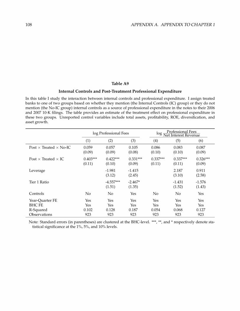
108 APPENDIX A. APPENDIX TO CHAPTER 1
Table A9
Internal Controls and Post-Treatment Professional Expenditure
In this table I study the interaction between internal controls and professional expenditure. I assign treatedbanks to one of two groups based on whether they mention (the Internal Controls (IC) group) or they do notmention (the No-IC group) internal controls as a source of professional expenditure in the notes to their 2006and 2007 10-K filings. The table provides an estimate of the treatment effect on professional expenditure inthese two groups. Unreported control variables include total assets, profitability, ROE, diversification, andasset growth.
log Professional Fees log Professional FeesNet Interest Revenue
(1) (2) (3) (4) (5) (6)
Post × Treated × No-IC 0.059 0.057 0.105 0.086 0.083 0.087(0.09) (0.09) (0.08) (0.10) (0.10) (0.09)
Post × Treated × IC 0.403*** 0.422*** 0.331*** 0.337*** 0.337*** 0.326***(0.11) (0.10) (0.09) (0.11) (0.11) (0.09)
Leverage -1.981 -1.415 2.187 0.911(3.12) (2.45) (3.10) (2.58)
Tier 1 Ratio -4.557*** -2.467* -1.431 -1.576(1.51) (1.35) (1.52) (1.43)
Controls No No Yes No No Yes
Year-Quarter FE Yes Yes Yes Yes Yes YesBHC FE Yes Yes Yes Yes Yes YesR-Squared 0.102 0.128 0.187 0.054 0.068 0.127Observations 923 923 923 923 923 923
Note: Standard errors (in parentheses) are clustered at the BHC-level. ***, **, and * respectively denote sta-tistical significance at the 1%, 5%, and 10% levels.

A.3. ADDITIONAL RESULTS: MANAGEMENT MONITORING 109
Table A10
SEC Accelerated Filers
In this table, I investigate whether the observed changes in valuation and professional expenses after the tre-atment are due to size-related SOX provisions as opposed to the Fed policy. Similar to Iliev (2010), in Panel A Irun a falsification test to investigate whether SEC resolution 70 FR 56825 (allowing small, non-accelerated SECfilers to postpone the implementation of SOX) has a valuation impact on non-accelerated SEC filers after thefirst quarter of 2006. In Panel B, I similarly investigate whether the treatment effect on professional fees comesfrom the subset of treated BHCs that are non-accelerated filers. Unreported control variables include leverage,Tier 1 Ratio, profitability, ROE, diversification, and asset growth.
Panel A: Accelerated Filers vs. Non-Accelerated Filers
log Tobin’s q log Market-to-Book log Prof. Fees log Prof. FeesNet Int. Income
(1) (2) (3) (4) (5) (6) (7) (8)
Post × Nonacc. Filer -0.004 -0.005 -0.021 -0.036 0.128 0.111 0.108 0.118(0.00) (0.00) (0.02) (0.02) (0.08) (0.08) (0.09) (0.08)
Controls No Yes No Yes No Yes No Yes
Year-Quarter FE Yes Yes Yes Yes Yes Yes Yes YesBHC FE Yes Yes Yes Yes Yes Yes Yes YesR-Squared 0.039 0.090 0.061 0.217 0.031 0.077 0.043 0.106Observations 985 985 985 985 461 461 461 461
Panel B: Interaction Effects, Treated × Accelerated Filers
log Tobin’s q log Market-to-Book log Prof. Fees log Prof. FeesNet Int. Income
(1) (2) (3) (4) (5) (6) (7) (8)
Post × Nonacc. Treated -0.011*** -0.011*** -0.055** -0.077*** 0.246*** 0.213** 0.207** 0.227***(0.00) (0.00) (0.02) (0.02) (0.08) (0.08) (0.09) (0.08)
Post × Acc. Treated -0.026*** -0.027*** -0.130*** -0.142*** 0.204 0.214 0.225 0.201(0.01) (0.01) (0.05) (0.04) (0.15) (0.15) (0.16) (0.15)
Controls No Yes No Yes No Yes No Yes
Year-Quarter FE Yes Yes Yes Yes Yes Yes Yes YesBHC FE Yes Yes Yes Yes Yes Yes Yes YesR-Squared 0.099 0.153 0.098 0.262 0.056 0.097 0.062 0.124Observations 1,025 1,025 1,025 1,025 480 480 480 480
Note: Standard errors (in parentheses) are clustered at the BHC-level. ***, **, and * respectively denote sta-tistical significance at the 1%, 5%, and 10% levels.

110 APPENDIX A. APPENDIX TO CHAPTER 1
Table A11
Summary Statistics: Funding Costs, Profitability, and Earnings Smoothing
This table reports summary statistics for the dependent variables used in Section 1.5.1, both in the 2006-2008full sample and in the two sub-samples of banks with total assets below $500 million and with total assetsbetween $500 and $700 million (the “unmonitored” and “monitored” groups, respectively). In the table, LLPstands for Loan Loss Provisions, while DNLLP stands for Discretionary Negative Loan Loss Provisions (seeTable 1.6). All the variables are constructed using data from quarterly Compustat Bank, and are reported inpercentage terms.
2006-2008 Sample Unmonitored Monitored
N Mean Med. SD N Mean Med. SD N Mean Med. SD
Int. Expense/Total Loans 1,129 1.02 0.99 0.32 625 1.01 0.98 0.36 504 1.02 1.00 0.27Int. Income/Total Loans 1,128 2.30 2.21 0.50 625 2.33 2.22 0.59 503 2.25 2.21 0.36ROE 1,067 1.24 1.99 3.89 613 1.01 1.92 3.97 454 1.54 2.13 3.75LLP/Net Interest Income 1,110 0.00 0.00 0.03 612 0.00 0.00 0.03 498 0.00 0.00 0.02DNLLP 1 645 6.55 4.61 6.33 359 6.68 4.64 6.38 286 6.38 4.49 6.28DNLLP 2 651 6.62 4.57 6.33 364 6.70 4.75 6.36 287 6.51 4.41 6.30

A.3. ADDITIONAL RESULTS: MANAGEMENT MONITORING 111
Table A12
Funding Costs and Earnings Smoothing: Robustness and Placebo
In this table, I show two sets of robustness test on the results of Table 1.6. In Panel A, I show changes in thefunding costs (interest expense divided by interest income, Specification (1), and interest expense divided bytotal loans, Specification (2)), profitability (ROA and ROE), LLP (LLP to loans, Specification (5), and LLP tonet interest income, Specification (6)), and discretionary LLP (DLLP 1 and 2) of unmonitored banks duringthe financial crisis, where I restrict the sample to banks that survive for the entire 2006-2008 period. In PanelB, I use an alternative threshold of $400 million to define unmonitored banks. Unreported controls includeprevious-quarter Tobin’s q, leverage, Tier 1 Ratio, total assets, diversification, and asset growth in the first fourspecifications of both panels, as well as operating profitability and ROE in the last four specifications.
Panel A: Surviving Banks
Funding Costs ROA/ROE LLP DNLLP
(1) (2) (3) (4) (5) (6) (7) (8)
Crisis × Unmonitored 0.033 0.061** -0.080 -0.088 -0.519*** -0.553** 0.463* 0.619**(0.02) (0.02) (0.10) (0.10) (0.19) (0.22) (0.25) (0.26)
Controls Yes Yes Yes Yes Yes Yes Yes Yes
Year-Quarter FE Yes Yes Yes Yes Yes Yes Yes YesBHC FE Yes Yes Yes Yes Yes Yes Yes YesR-Squared 0.578 0.756 0.261 0.233 0.416 0.562 0.379 0.385Observations 645 645 560 560 433 433 409 417
Panel B: $400M Monitoring Threshold Placebo Sample
Funding Costs ROA/ROE LLP DNLLP
(1) (2) (3) (4) (5) (6) (7) (8)
Crisis × Small 0.011 0.031 -0.140 -0.156 -0.144 -0.078 0.379 0.492(0.02) (0.03) (0.13) (0.13) (0.26) (0.29) (0.27) (0.30)
Controls Yes Yes Yes Yes Yes Yes Yes Yes
Year-Quarter FE Yes Yes Yes Yes Yes Yes Yes YesBHC FE Yes Yes Yes Yes Yes Yes Yes YesR-Squared 0.513 0.748 0.254 0.236 0.350 0.526 0.340 0.318Observations 911 911 783 783 630 630 541 553
Note: Standard errors (in parentheses) are clustered at the BHC-level. ***, **, and * respectively denote sta-tistical significance at the 1%, 5%, and 10% levels.

112 APPENDIX A. APPENDIX TO CHAPTER 1
Table A13
Robustness: Cash Flow Risk, Shareholder Value, and Professional Expenditure
In this table I perform a robustness check on the results of Table 1.7 by using alternative risk measures to sorttreated banks. In Panel A I sort treated banks based on whether their average Z-Score is above or below themedian Z-Score in my sample. Similarly, in Panel B I sort treated banks based on whether their average equityvolatility is above or below the median equity volatility in my sample. Both Z-Score and equity volatility aredefined as in Table 1.5. Unreported control variables include leverage, Tier 1 Ratio, total assets, profitability,ROE, diversification and asset growth.
Panel A: Z-Score Sorting
log Tobin’s q log Market-to-Book log Prof. Fees
(1) (2) (3) (4) (5) (6)
Post × Treated × Low Z-Score -0.008 -0.008* -0.050 -0.058* 0.244* 0.215**(0.00) (0.00) (0.03) (0.03) (0.14) (0.09)
Post × Control × High Z-Score -0.012*** -0.013*** -0.086*** -0.088*** 0.272*** 0.269***(0.00) (0.00) (0.03) (0.03) (0.09) (0.09)
Controls No Yes No Yes No Yes
Year-Quarter FE Yes Yes Yes Yes Yes YesBHC FE Yes Yes Yes Yes Yes YesR-Squared 0.361 0.419 0.414 0.504 0.076 0.182Observations 2,177 2,177 2,177 2,177 999 999
Panel B: Equity Volatility Sorting
log Tobin’s q log Market-to-Book log Prof. Fees
(1) (2) (3) (4) (5) (6)
Post × Treated × Low Volatility -0.006 -0.007 -0.027 -0.041 0.320*** 0.267***(0.00) (0.00) (0.03) (0.03) (0.10) (0.09)
Post × Treated × High Volatility -0.012*** -0.013*** -0.095*** -0.094*** 0.212* 0.227***(0.00) (0.00) (0.03) (0.03) (0.12) (0.08)
Controls No Yes No Yes No Yes
Year-Quarter FE Yes Yes Yes Yes Yes YesBHC FE Yes Yes Yes Yes Yes YesR-Squared 0.360 0.417 0.416 0.505 0.079 0.183Observations 2,160 2,160 2,160 2,160 995 995
Note: Standard errors (in parentheses) are clustered at the BHC-level. ***, **, and * respectively denote sta-tistical significance at the 1%, 5%, and 10% levels.

A.3. ADDITIONAL RESULTS: MANAGEMENT MONITORING 113
Table A14
Chairman Ownership and Professional Expenditure Persistence
This table shows the persistence of the treatment effect on professional expenditure for treated banks withchairman ownership in the bottom two terciles of the chairman ownership distribution in my sample, as wellas in the top tercile of the distribution. The independent variable is the natural logarithm of professionalexpenditures. Unreported control variables include leverage, Tier 1 Ratio, total assets, profitability, ROE, di-versification and asset growth.
Low Chairman Own. Treated High Chairman Own. Treated
(1) (2) (3) (4) (5) (6)
Q1-2006 × Treated 0.148 0.160* 0.173* 0.272** 0.293*** 0.238**(0.10) (0.09) (0.09) (0.11) (0.10) (0.09)
Q2-2006 × Treated 0.288** 0.280** 0.290*** 0.395*** 0.404*** 0.314**(0.11) (0.11) (0.11) (0.14) (0.13) (0.12)
Q3-2006 × Treated 0.144 0.153 0.150 0.406*** 0.429*** 0.337***(0.11) (0.10) (0.10) (0.13) (0.13) (0.12)
Q4-2006 × Treated 0.033 0.020 0.027 0.421*** 0.424*** 0.328**(0.12) (0.11) (0.11) (0.16) (0.15) (0.16)
Q1-2007 × Treated 0.210* 0.196* 0.209** 0.484*** 0.486*** 0.389**(0.12) (0.12) (0.10) (0.18) (0.16) (0.16)
Q2-2007 × Treated 0.275** 0.277** 0.265*** 0.511*** 0.531*** 0.414***(0.13) (0.12) (0.10) (0.17) (0.15) (0.13)
Q3-2007 × Treated 0.351** 0.344*** 0.343*** 0.530*** 0.541*** 0.447***(0.14) (0.13) (0.10) (0.18) (0.16) (0.14)
Q4-2007 × Treated 0.198 0.188 0.167 0.338 0.333 0.259(0.20) (0.20) (0.17) (0.27) (0.25) (0.24)
Controls No Yes Yes No Yes Yes
Year-Quarter FE Yes Yes Yes Yes Yes YesBHC FE Yes Yes Yes Yes Yes YesR-Squared 0.069 0.098 0.173 0.120 0.137 0.190Observations 875 875 875 667 667 667
Note: Standard errors (in parentheses) are clustered at the BHC-level. ***, **, and * respectively denote sta-tistical significance at the 1%, 5%, and 10% levels.

114 APPENDIX A. APPENDIX TO CHAPTER 1
Table A15
Chairman Ownership and Market-to-Book Discount Persistence
This table shows the persistence of the treatment effect on Market-to-Book for treated banks with chairmanownership in the bottom two terciles of the chairman ownership distribution in my sample, as well as in the toptercile of the distribution. The independent variable is the natural logarithm of Market-to-Book. Unreportedcontrol variables include leverage, Tier 1 Ratio, total assets, profitability, ROE, diversification and asset growth.
Low Chairman Own. Treated High Chairman Own. Treated
(1) (2) (3) (4) (5) (6)
Q1-2006 × Treated -0.045* -0.053** -0.051** -0.052* -0.067** -0.056**(0.02) (0.02) (0.02) (0.03) (0.03) (0.03)
Q2-2006 × Treated -0.061** -0.069** -0.068** -0.061* -0.075** -0.064*(0.03) (0.03) (0.03) (0.03) (0.03) (0.03)
Q3-2006 × Treated -0.068** -0.075** -0.076*** -0.075** -0.096*** -0.084**(0.03) (0.03) (0.03) (0.04) (0.03) (0.03)
Q4-2006 × Treated -0.067** -0.069** -0.069** -0.063 -0.085** -0.071*(0.03) (0.03) (0.03) (0.04) (0.04) (0.04)
Q1-2007 × Treated -0.069** -0.072** -0.070** -0.055 -0.075** -0.066*(0.03) (0.03) (0.03) (0.04) (0.04) (0.03)
Q2-2007 × Treated -0.060 -0.070** -0.070** -0.052 -0.082* -0.074*(0.04) (0.04) (0.03) (0.05) (0.05) (0.04)
Q3-2007 × Treated -0.075* -0.075** -0.070** -0.049 -0.082* -0.061(0.04) (0.04) (0.03) (0.05) (0.04) (0.04)
Q4-2007 × Treated -0.094* -0.094** -0.090** -0.059 -0.086 -0.077(0.05) (0.04) (0.04) (0.06) (0.05) (0.05)
Controls No Yes Yes No Yes Yes
Year-Quarter FE Yes Yes Yes Yes Yes YesBHC FE Yes Yes Yes Yes Yes YesR-Squared 0.425 0.484 0.513 0.410 0.474 0.524Observations 1,910 1,910 1,910 1,503 1,503 1,503
Note: Standard errors (in parentheses) are clustered at the BHC-level. ***, **, and * respectively denote sta-tistical significance at the 1%, 5%, and 10% levels.

A.4. TESTS OF ADDITIONAL HYPOTHESES 115
A.4 Tests of Additional Hypotheses
Table A16
Government Tail Risk Insurance
In this table, I investigate the treatment effect on treated banks’ exposure to bank-specific tail risk (Gandhi andLustig (2015)). In each quarter from Q1-2004 to Q4-2008, I sort commercial bank stocks into five size portfoliosbased on their market capitalization at the end of the previous quarter. I compute daily value-weighted excessreturns on each of the five size portfolios, and regress these daily excess returns on the Fama-French market, hmland smb risk factors (from Kenneth French’s website), and two factors measuring bank interest rate risk (ltg,the yield on a 10-year treasury note minus the yield on a 2-year treasury note) and credit risk (crd, the Moody’sSeasoned Aaa Corporate Bond Yield index minus the yield on a 10-year treasury note). The data used toconstruct ltg and crd comes from the Federal Reserve of St. Louis’ website. I combine the residuals from thetime-series regressions in a (Td × 5) matrix (where Td is the number of daily portfolio return observations forthe period 2004-2007), and obtain the size factor as the second principal component of this matrix. The tableshows the treatment effect on the quarterly loading of each bank’s excess returns on the size risk factor. Theloadings I use as dependent variables in the first three specifications come from the market model augmentedwith the bank size factor, while the loadings in the last three specifications come from the Gandhi-Lustig (GL)specification that includes the bank size factor and the other orthogonal factors (market, hml, smb, ltg and crd)as risk factors. The unreported liquidity controls include all the liquidity variables from Table A18, Panel A.The remaining unreported controls include leverage, Tier 1 Ratio, profitability, ROE, diversification, and assetgrowth.
Factor Loading (Market Model) Factor Loading (GL Model)
(1) (2) (3) (4) (5) (6)
Post × Treated 0.000 0.001 0.000 0.000 0.001 0.000(0.00) (0.00) (0.00) (0.00) (0.00) (0.00)
Liquidity Controls No Yes Yes No Yes Yes
Other Controls No No Yes No No Yes
Year-Quarter FE Yes Yes Yes Yes Yes YesBHC FE Yes Yes Yes Yes Yes YesR-Squared 0.016 0.025 0.047 0.014 0.021 0.039Observations 2,044 2,044 2,044 2,044 2,044 2,044
Note: Standard errors (in parentheses) are clustered at the BHC-level. ***, **, and * respectively denote sta-tistical significance at the 1%, 5%, and 10% levels.

116 APPENDIX A. APPENDIX TO CHAPTER 1
Table A17
Voluntary Reporting
This table compares the treatment effect on Tobin’s q (Panel A) and Market-to-Book (Panel B) across two sub-groups of treated BHCs. The first sub-group consists of treated BHCs that voluntarily file form FR Y-9C afterthe treatment. The second sub-group consists of treated BHCs that stop filing form FR Y-9C after the treatment.Unreported control variables include professional fees, profitability, ROE, diversification, and asset growth.
Panel A: log Tobin’s q Regressions
Voluntary Reporting Not Reporting
(1) (2) (3) (4) (5) (6)
Post × Treated -0.012** -0.012*** -0.012*** -0.010** -0.011*** -0.010***(0.00) (0.00) (0.00) (0.00) (0.00) (0.00)
Leverage 0.395** 0.311** 0.291** 0.211*(0.15) (0.13) (0.13) (0.11)
Tier 1 Ratio 0.489*** 0.366*** 0.293*** 0.184***(0.11) (0.11) (0.07) (0.06)
Other Controls No No Yes No No Yes
Year-Quarter FE Yes Yes Yes Yes Yes YesBHC FE Yes Yes Yes Yes Yes YesR-Squared 0.360 0.404 0.425 0.353 0.374 0.407Observations 1,412 1,412 1,412 1,922 1,922 1,922
Panel B: log Market-to-Book Regressions
Voluntary Reporting Not Reporting
(1) (2) (3) (4) (5) (6)
Post × Treated -0.082* -0.089** -0.084** -0.078*** -0.084*** -0.075***(0.04) (0.03) (0.04) (0.03) (0.03) (0.02)
Leverage 5.873*** 5.307*** 5.215*** 4.868***(0.94) (0.88) (0.91) (0.74)
Tier 1 Ratio 3.053*** 2.236*** 2.062*** 1.094**(0.71) (0.73) (0.48) (0.42)
Other Controls No No Yes No No Yes
Year-Quarter FE Yes Yes Yes Yes Yes YesBHC FE Yes Yes Yes Yes Yes YesR-Squared 0.420 0.487 0.503 0.407 0.462 0.512Observations 1,412 1,412 1,412 1,922 1,922 1,922
Note: Standard errors (in parentheses) are clustered at the BHC-level. ***, **, and * respectively denote sta-tistical significance at the 1%, 5%, and 10% levels.

A.4. TESTS OF ADDITIONAL HYPOTHESES 117
Table A18
Liquidity, Volatility, and Market Frictions
In this table, I study the treatment effect on liquidity, volatility, and market information responsiveness oftreated banks’ stocks. In Panel A, I show the treatment effect on the Holden (2009) Effective Tick Size, theCorwin and Schultz (2012) Bid-Ask Spread, and the Amihud (2002) liquidity measures (constructed as in thereferenced papers). Moreover, I show the effect on Zero Days Traded (number of days in which a stock is nottraded) and Turnover (daily volume divided by shares outstanding). Effective Tick Size and Zero Days Tradedare computed on a quarterly basis, while Bid-Ask Spread, Amihud and Turnover are quarterly averages ofdaily measures. In Panel B, I show the treatment effect on quarterly return volatility, quarterly idiosyncraticvolatility (IdVol) from the Fama-French four factor model (FF4), and quarterly idiosyncratic volatility fromthe Adrian et al. (2015) Financial CAPM model (FCAPM). Finally, in Specifications (7)-(10) I show the effecton quarterly measures of price responsiveness to market information (D1 and D2, as in Hou and Moskowitz(2005)). All the variables used in the table are constructed using daily stock returns from CRSP. The controlvariables in Panels A and B include leverage, Tier 1 Ratio, profitability, ROE, diversification, and asset growth.Moreover, Panel B includes all the liquidity variables from Panel A as additional controls.
Panel A: Liquidity
Effective Tick CS Spread Amihud Zero Days Turnover
(1) (2) (3) (4) (5) (6) (7) (8) (9) (10)
Post × Treated -0.000 -0.000 -0.003 -0.003 0.000* 0.000* 0.006 0.001 -0.000 -0.000(0.00) (0.00) (0.00) (0.00) (0.00) (0.00) (0.01) (0.01) (0.00) (0.00)
Controls No Yes No Yes No Yes No Yes No Yes
Year-Quarter FE Yes Yes Yes Yes Yes Yes Yes Yes Yes YesBHC FE Yes Yes Yes Yes Yes Yes Yes Yes Yes YesR-Squared 0.037 0.089 0.252 0.299 0.043 0.054 0.082 0.118 0.049 0.097Observations 2,044 2,044 2,044 2,044 2,044 2,044 2,044 2,044 2,044 2,044
Panel B: Equity Volatility and Market Delay
Total Vol FF4 IdVol FCAPM IdVol D1 D2
(1) (2) (3) (4) (5) (6) (7) (8) (9) (10)
Post × Treated -0.001 -0.001 -0.001 -0.001 -0.001 -0.001 0.040* 0.030 0.245 0.222(0.00) (0.00) (0.00) (0.00) (0.00) (0.00) (0.02) (0.02) (0.40) (0.39)
Liquidity Controls No Yes No Yes No Yes No Yes No Yes
Other Controls No Yes No Yes No Yes No Yes No Yes
Year-Quarter FE Yes Yes Yes Yes Yes Yes Yes Yes Yes YesBHC FE Yes Yes Yes Yes Yes Yes Yes Yes Yes YesR-Squared 0.212 0.629 0.208 0.608 0.205 0.610 0.018 0.040 0.013 0.021Observations 2,044 2,044 2,044 2,044 2,044 2,044 2,044 2,044 2,044 2,044
Note: Standard errors (in parentheses) are clustered at the BHC-level. ***, **, and * respectively denote sta-tistical significance at the 1%, 5%, and 10% levels.

118 APPENDIX A. APPENDIX TO CHAPTER 1
Table A19
Leverage and Capital Ratios
In this table, I investigate the treatment effect on bank leverage and capital requirements. In Panel A, I investi-gate the treatment effect on three different measures of bank leverage, namely liabilities divided by total assets,divided by the book value of equity and divided by total earning assets (the sum of cash and due from banks,assets sold under repurchase agreements, trading account securities, investment securities, loans net of loanloss allowance, customer acceptances, and other assets). In Panel B, I investigate the treatment effect on theTier 1, Tier 2 and Combined (Tier 1 plus Tier 2) Capital Ratio of treated banks. The Tier 1 Ratio is the sum ofequity capital and minority interests, divided by risk-weighted assets. The Tier 2 Ratio is the sum of cumula-tive preferred stock, qualifying debt, and allowance for credit losses minus investment in certain subsidiaries,divided by risk-weighted assets. Unreported control variables include profitability, ROE, diversification, andasset growth.
Panel A: Leverage
log LiabilitiesAssets log Liabilities
Equity log LiabilitiesEarning Assets
(1) (2) (3) (4) (5) (6)
Post × Treated -0.001 -0.001 -0.009 -0.012 -0.002 -0.002(0.00) (0.00) (0.03) (0.03) (0.00) (0.00)
Controls No Yes No Yes No Yes
Year-Quarter FE Yes Yes Yes Yes Yes YesBHC FE Yes Yes Yes Yes Yes YesR-Squared 0.012 0.048 0.014 0.073 0.038 0.111Observations 2,575 2,575 2,575 2,575 2,575 2,575
Panel B: Capital Ratios
log Tier 1 Ratio log Tier 2 Ratio log Combined Ratio
(1) (2) (3) (4) (5) (6)
Post × Treated 0.026 0.033 -0.064 -0.065 0.007 0.013(0.02) (0.02) (0.05) (0.05) (0.02) (0.02)
Controls No Yes No Yes No Yes
Year-Quarter FE Yes Yes Yes Yes Yes YesBHC FE Yes Yes Yes Yes Yes YesR-Squared 0.028 0.175 0.050 0.056 0.062 0.176Observations 2,178 2,178 2,159 2,159 2,199 2,199
Note: Standard errors (in parentheses) are clustered at the BHC-level. ***, **, and * respectively denote sta-tistical significance at the 1%, 5%, and 10% levels.

Appendix B
Appendix to Chapter 2
119

120 APPENDIX B. APPENDIX TO CHAPTER 2
B.1 Substitutability and Price Externalities
In this Appendix extend the analysis of Section 2.3 by allowing for a rich degree of price externa-
lities. In particular, we analyze the degree to which the ability of the Principal to impose group
punishments improves social welfare when varying the degree of substitutability between the out-
put of individual producers. In Section B.1.1, we introduce a new pricing function which admits
a variable degree of substitution across producers’ goods and derive equilibrium outcomes of the
stage game. In Section B.1.2, we develop a recursive formulation of the infinite-horizon game and
show that the usefulness of group punishments increases as goods become more substitutable.
B.1.1 Stage Game
We generalize the price function by assuming that consumers have Cobb-Douglas preferences over
a bundle of individual producers’ output and a numeraire good, and that these consumers face taxes
τ on purchases of each producers’ output. In this economy, the inverse demand function for each
producer i’s output satisfies
pi (q, τ) = αqρ−1
i
∑ni=1 qρ
i− τ, (B.1)
where α ∈ (0, 1) and ρ ∈ (0, 1). Here, the parameter α is a Cobb-Douglas parameter that governs
the substitutability between the numeraire good and the bundle of producers’ output, while the
parameter ρ governs the degree of substitutability between each producer’s output. Under this
formulation, a higher level of ρ implies a higher degree of substitutability.
With prices specified in (B.1), each producer i obtains a static payoff given by
ui (q, τ) = αqρ
i
∑ni=1 qρ
i− τqi − cqi, (B.2)
while the Principal obtains a static payoff given by
w (Q, τ) =n
∑i=1
pi(q, τ)qi (B.3)
= α− τQ. (B.4)

B.1. SUBSTITUTABILITY AND PRICE EXTERNALITIES 121
As in the case of a linear inverse demand function, after observing any level Q, the Principal op-
timally chooses τ (Q) = 0 in the stage game. We impose a restriction on the strategy set of each
producer which requires strictly positive production. Formally, we restrict qi ∈[q, ∞
]with q < qN
i .
Under this restriction, the level of output that maximizes joint profits in the stage game satisfies
qmi = arg max
qi≥q
(α
n− cqi
)(B.5)
= q. (B.6)
Next, to solve for the unique perfect-public equilibrium of the stage game qNi , we note that for each
q−i, producer i solves
maxqi
αqρ
i
qρi + ∑−i qρ
−i− cqi.
It is straightforward to show that the unique perfect-public equilibrium of the stage game is
qNi =
n− 1n2
αρ
c. (B.7)
B.1.2 Infinitely-Repeated Game
We focus on characterizing strongly symmetric perfect-public equilibria. We denote by u (q, τ) the
producer’s payoff and by w (Q, τ) the Principal’s payoff, and after appealing to the one-shot devia-
tion principle, we proceed to characterize the best and worst perfect-public equilibria of the repeated
game. Under the inverse demand function (B.1), for a given level of the worst equilibrium payoff v
the best equilibrium payoff v solves
v = maxq
u (q, 0) ,
subject to, for all q′,
u (q, 0) ≥ (1− δ) g(q′, q, τ
(q′ + (n− 1) q
))+ δv, (B.8)
v ≥ 1− δ
δ
1n[w(q′ + (n− 1) q, 0
)− w
(q′ + (n− 1) q, τ
(q′ + (n− 1) q
))]+ v, (B.9)

122 APPENDIX B. APPENDIX TO CHAPTER 2
where g (q′, q, τ (q′ + (n− 1) q)) now satisfies
g(q′, q, τ
(q′ + (n− 1) q
))= u
(q′, q, τ
(q′ + (n− 1) q
)]+
1n
w(q′ + (n− 1) q, 0
)− 1
nw(q′ + (n− 1) q, τ
(q′ + (n− 1) q
)). (B.10)
As in the previous section, we define the maximum payoff that can be achieved by a producer by
deviating to q′ when the others are producing q as g (q, τ (·)). This maximum payoff satisfies
g (q, τ (·)) = maxq′
g(q′, q, τ(q′ + (n− 1)q)
).
In the next lemma, we show that as long as the prescribed output is larger than the static Nash
equilibrium output, the maximum deviation payoff g(q, τ (·)) is minimized when the Principal levies
no taxes (i.e., when τ = 0).
Lemma 12. g (q, τ (·)) ≥ g (q, τ = 0) when q ≥ qN .
Proof. See Appendix B.2.2.
Given Lemma 12, the key propositions of Section 2.3 immediately extend to the environment with
imperfectly substitutable goods. Here, we explore how the usefulness of group punishments in
improving welfare depends on the degree of substitutability between individual producers’ output.
We start by showing in the following lemma that when the number of producers n is sufficiently
large, the best equilibrium level of output of the model where taxes are not allowed is increasing in
the substitutability parameter ρ.
Lemma 13. For n sufficiently large, dqA/dρ > 0.
Proof. See Appendix B.2.2.
The intuition behind this lemma is that when output is more substitutable the negative impact of
an individual producer’s output on the common price is lower. This increases producers’ incentives

B.1. SUBSTITUTABILITY AND PRICE EXTERNALITIES 123
to over-produce, and leads to higher levels of production and lower equilibrium values in the best
equilibrium.
Finally, in the following proposition we formalize our numerical illustration from Section 2.3.3 that
the welfare gains from group punishments are increasing in the parameter ρ. For a given set of
parameters, let ∆U denote the change in the value of the best equilibrium in our model relative to
the value of the best equilibrium in the model where group punishments are not allowed, i.e.
∆U ≡u (q)− u
(qA)
u (qA). (B.11)
Proposition 14. Fix ρ ∈ (0, 1). For n sufficiently large, there exists a δ ∈ (0, 1) and ρ > 0 such that for all
ρ′ ∈ (ρ, ρ), d∆U (ρ′) /dρ′ > 0.
We give here a sketch of our argument, and leave a formal proof to Appendix B.2.2. For a fixed level
of the substitutability parameter ρ, we know that our model achieves the first-best level of output
qm at a lower level of the discount factor than the model where taxes are not allowed. This happens
because, as showed in Proposition 8, the threat of taxes always weakly enlarges the equilibrium
set, and strictly enlarges the equilibrium set when producers are sufficiently patient. We denote by
δA∗(ρ) the threshold level of the discount factor at which the model where taxes are not allowed
first achieves qm as the most collusive level of output, and by δ∗(ρ) the level of the discount factor
at which our model first achieves qm as the most collusive level of output. Since δ∗(ρ) < δA∗(ρ), we
can always find a discount factor δ0 such that δ∗(ρ) < δ0 < δA∗(ρ). At δ0 the model where taxes
are allowed achieves qm as the most collusive level of output, while the model where taxes are not
allowed achieves a higher level of output (a lower value) than qm. In the final step of the proof we
argue that by continuity at this δ0, if ρ increases by a sufficiently small amount to some ρ′ > ρ, the
model where taxes are allowed still achieves qm as the most collusive level of output. At δ0, on the
other hand, the most collusive level of output under ρ′ is strictly greater than the most collusive level
of output under ρ in the model where taxes are not allowed (from Lemma 13). Therefore the increase
in output (and decrease in value) relative to qm (the most collusive level of output at δ0, in the model
where taxes are allowed) increases when ρ increases to ρ′. Using the same argument, we prove that
for all ρ′ ∈ (ρ, ρ), d∆U (ρ′) /dρ′ > 0.

124 APPENDIX B. APPENDIX TO CHAPTER 2
Figure B1
Comparative Statics: Marginal Costs of Production and Team Welfare
Percentage increase in welfare in best equilibrium from group punishments for various marginal costs of pro-duction c for a fixed discount factor (δ = 0.16).
Goods Substitutability (ρ)0.3 0.35 0.4 0.45 0.5 0.55 0.6 0.65 0.7 0.75 0.8
% W
elfa
re C
hang
e
0.04
0.06
0.08
0.1
0.12
0.14
0.16
c = 0.1c = 0.5c = 0.8c = 1
Different parametrizations of the model suggest that the results of Proposition 14 hold for a wide
range of the model’s key parameters. As an example, Figure B1 shows the percentage increase in
welfare in the best equilibrium associated with group punishments for various values of the degree
of substitutability ρ and the marginal cost of production, c. In this figure, we hold the discount factor
fixed at a value of δ = 0.16. This figure clearly shows that an increase in the degree of substitutability
strictly raises the welfare gains associated with group punishments and that these welfare gains are
not particularly sensitive to the marginal costs of production.
B.2 Definitions and Proofs
B.2.1 Definitions and Proofs from Sections 2.2 and 2.3
Repeated Game Definitions
Definition 1. For any history hwt ∈ Hw the continuation game is the infinitely-repeated game that be-
gins in period t, following history hwt. For any strategy profile σ =({σi}n
i=1 , σw), agent i’s continuation

B.2. DEFINITIONS AND PROOFS 125
strategy induced by hwt is given by σi(hwthws) for all hws ∈ Hw, where hwthws is the concatenation of his-
tory hwt followed by history hws. Similarly, the Principal continuation strategy induced by hwt is given by
σw((
hwthws) , x(σ1(hwthws) , σ2
(hwthws) , . . . , σn
(hwthws))) for all hws ∈ Hw.
Definition 2. A Perfect-Public Equilibrium is σ =({σi}n
i=1 , σw)
such that, for all histories hwt ∈ Hw,
Uti(hwt, σ
)≥ Ut
i(hwt, (σi, σ−i, σw)
)(B.12)
for all i, σi, and
Utw(hwt, σ
)≥ Ut
w(hwt,
({σi}n
i=1 , σw))
(B.13)
for all σw.
Definition 3. A one-shot deviation for agent i from strategy σi is a strategy σi 6= σi such that there exists a
unique history hwt ∈ Hw such that for all hws 6= hwt,
σi (hws) = σi (hws) . (B.14)
Similarly, a one-shot deviation for the Principal from strategy σw is a strategy σw 6= σw such that for all
hwt ∈ Hw there exists a level of the total outcome xt such that for all xt 6= xt,
σw(hwt, xt
)= σw
(hwt, xt
). (B.15)
Definition 4. A one-shot deviation σi from the agent strategy σi is profitable if at history hwt for which
σi(hwt) 6= σi
(hwt),
Uti(hwt, (σi, σ−i, σw)
)> Ut
i(hwt, σ
). (B.16)
A one-shot deviation σw from the Principal strategy σw is profitable if for all hwt ∈ Hw, at the outcome level
for which σw(hwt, xt
)6= σw
(hwt, xt
),
Utw(hwt,
({σi}n
i=1 , σw))
> Utw(hwt, σ
). (B.17)

126 APPENDIX B. APPENDIX TO CHAPTER 2
Proof of Proposition 3
If a profile is perfect-public, clearly there are no profitable one-shot deviations. Now suppose that the
profile σ is not perfect-public. We want to show that there must be a profitable one-shot deviation.
Since σ is not perfect-public, there exists a history hwt, an agent i and a strategy σi (the proof for the
Principal follows the same steps) such that
Uti(hwt, σ
)< Ut
i(hwt, (σi, σ−i, σw)
). (B.18)
Let ε = Uit(hwt, (σi, σ−i, σw)
)−Ui
t(hwt, σ
). Let m = mini,q,τ ui (q, τ) and M = maxi,q,τ ui (q, τ), with T
large enough that δT (M−m) < ε/2.B.1. Finally, for any agent i and history hws ∈ Hw, let
usi((
hwthws) , σ)
= ui
({σi(hwthws)}n
i=1 , σw((
hwthws) , x(hwthws))) , (B.19)
where x(hwthws) is short-hand notation for x
(σ1(hwthws) , σ2
(hwthws) , . . . , σn
(hwthws)), and denote
by hws the period-s history induced by (σi, σ−i, σw). Then,
(1− δ)
[T−1
∑s=t
δsusi((
hwthws) , σ)
+∞
∑s=T
δsusi((
hwthws) , σ)]
= (1− δ)
[T−1
∑s=0
δsusi((
hwthws) , (σi, σ−i, σw))
+∞
∑s=T
δsusi((
hwthws) , (σi, σ−i, σw))]− ε, (B.20)
so that
(1− δ)T−1
∑s=t
δsusi((
hwthws) , σ)
< (1− δ)T−1
∑s=0
δsusi((
hwthws) , (σi, σ−i, σw))− ε
2. (B.21)
Then the strategy σi such that
σi (hws) =
σi (hws) if s < T,
σi (hws) if s ≥ T,(B.22)
B.1Note that ui (·) is potentially unbounded below. Here we impose that m is an arbitrarily large negative number.

B.2. DEFINITIONS AND PROOFS 127
is a profitable deviation from σi(hwt). Now let hw(T−1) denote the period T − 1 history induced by
(σi, σ−i, σw). There are two possibilities. First, suppose
UT−1i
((hwthw(T−1)
), σ)
< UT−1i
((hwthw(T−1)
), (σi, σ−i, σw)
). (B.23)
Then, since σi agrees with σi in period T and after T, we have a profitable one-shot deviation after
history hwthw(T−1). Alternatively, suppose
UT−1i
((hwthw(T−1)
), σ)≥ UT−1
i
((hwthw(T−1)
), (σi, σ−i, σw)
), (B.24)
and construct the strategy
σi (hws) =
σi (hws) if s < T − 1,
σi (hws) if s ≥ T − 1.(B.25)
Since
UT−2i
((hwthw(T−2)
), (σi, σ−i, σw)
)= (1− δ) uT−2
i
((hwthw(T−2)
), (σi, σ−i, σw)
)+ δUT−1
i
((hwthw(T−1)
), (σi, σ−i, σw)
)(B.26)
≤ (1− δ) uT−2i
((hwthw(T−2)
), (σi, σ−i, σw)
)+ δUT−1
i
((hwthw(T−1)
), σ)
(B.27)
= UT−2i
((hwthw(T−2)
), (σi, σ−i, σw)
), (B.28)
then
Uti(hwt, (σi, σ−i, σw)
)≤ Ut
i(hwt, (σi, σ−i, σw)
), (B.29)
and σi is a profitable deviation at hwt that only differs from σi in the first T − 1 periods. Proceeding
in this way, we find a profitable one-shot deviation.

128 APPENDIX B. APPENDIX TO CHAPTER 2
Proof of Proposition 6
We need only prove that for each v ∈ [v, v], there exists a perfect-public equilibrium strategy which
attains the value v. To construct such strategy, we start from the set of perfect-public equilibrium
strategies of the game where the Principal is not allowed to impose group punishments,[vA, vA]. We
know from Abreu (1986) that any equilibrium value v0 such that v0 ∈[vA, vA] can be achieved with
a perfect-public equilibrium strategy σ0. Under σ0, the Principal never imposes group punishments
and agents exert effort a0 such that u(a0) = v0 on path, and punish deviations by both Principal
and agents by reversion to the worst (carrot-and-stick) perfect-public equilibrium with value vA.
Therefore, we focus on characterizing the equilibrium strategies for the cases in which[vA, vA] ⊂
[v, v].
Consider a new strategy σ1. Define by aA the carrot output in the model where group punishments
are not allowed. Under σ1, for some ε1 > 0 agents choose a1 = aA + ε1 as long as the aggregate
outcome x1 is such that x1 = x(a1), and the Principal never imposes punishments. Suppose that
an agent deviates to some a′, such that the observed aggregate outcome is x1 = x(a′, a1). In this
case, the Principal imposes an arbitrarily small punishment τ1 (x1) > 0 such that the punishment is
feasible. That is, such that v1 (a′, a1, τ1 (x1)) ∈ [v, v], where
v1(
a′, a1, τ1(
x1))
≡ 1− δ
δ
1n
[w(
a′, a1, 0)− w
(a′, a1, τ1
(x1))]
. (B.30)
If an agent deviates and the Principal implements the prescribed punishment, then agents follow the
strategy σ1 (v1 (a′, a1, τ1 (x1))). Therefore, the continuation value promised to agents when one of
the agents deviates and the Principal imposes τ1 (x1) can be achieved with a perfect-public equili-
brium strategy. Conversely, deviations by agents followed by deviations by the Principal are punis-
hed by the worst perfect-public equilibrium strategy σ1 (vA). Clearly, this strategy is a perfect-public
equilibrium. Moreover, it achieves a value u(a1) ≡ v1 > vA.
Next, note that reversion to the perfect-public equilibrium v1 > vA allows to construct a new carrot-
and-stick strategy in which agents contribute an effort level a1 < aA for one period and then revert
to v1, with deviations from the prescription causing the prescription to be repeated. Moreover, note

B.2. DEFINITIONS AND PROOFS 129
that this new carrot-and-stick strategy has value v1 < vA. Hence, for any value v1 ∈[v1, v1], we can
find a perfect-public equilibrium strategy σ1 such that u(σ1) = v1.
Now take some k ≥ 2 and set[vk, vk
]such that
[v1, v1] ⊂ [
vk, vk]⊂ [v, v], and assume that for
any vk ∈[vk, vk
]we can construct a perfect-public equilibrium strategy σk such that u
(σk)
= vk.
Denote by ak the effort level with value vk, and construct a new strategy σk+1. Under σk+1, for some
εk+1 > 0 agents produce ak+1 = ak + εk+1 as long as the observed aggregate outcome xk+1 is such that
xk+1 = x(
ak+1)
, and the Principal never imposes punishments. Suppose that an agent deviates to
some a′, such that the observed aggregate outcome is xk+1 = x(
a′, ak+1)
. In this case, the Principal
imposes a punishment τk+1(
xk+1)
> 0 such that the punishment is feasible. That is, such that
vk+1(
a′, ak+1, τk+1(
xk+1))∈ [v, v], where
vk+1(
a′, ak+1, τk+1(
xk+1))
≡ 1− δ
δ
1n
[w(
a′, ak+1, 0)− w
(a′, ak+1, τk+1
(xk+1
))]. (B.31)
Note that since vk > v1, the range of punishments that can be sustained is larger than[0, supx1 τ1 (x1)].
If an agent deviates and the Principal implements the prescribed tax, then agents follow the stra-
tegy σk+1(
vk+1(
a′, ak+1, τk+1(
xk+1)))
. Therefore, the continuation value promised to agents when
one of the agents deviates and the Principal imposes τk+1(
xk+1)
can be achieved with a perfect-
public equilibrium strategy. Conversely, deviations by agents followed by deviations by the Princi-
pal are punished by the worst perfect-public equilibrium strategy σk+1(
vk)
. Clearly, this strategy
is a perfect-public equilibrium. Moreover, it achieves a value u(
ak+1)≡ vk+1 > vk. Next, note
that reversion to the perfect-public equilibrium vk+1 > vk allows to construct a new carrot-and-stick
strategy in which agents exert an effort level ak+1 > ak for one period and then revert to vk+1, with
deviations from the prescription causing the prescription to be repeated. Moreover, note that this
new carrot-and-stick strategy has value vk+1 < vk. Hence, for any value vk+1 ∈[vk+1, vk+1
], we can
find a perfect-public equilibrium strategy σk+1 such that u(
σk+1)
= vk+1. The proof is completed by
induction.

130 APPENDIX B. APPENDIX TO CHAPTER 2
Proof of Proposition 7
Suppose σ ((a, a) , (0, 0)) is an optimal carrot-and-stick punishment. Recalling from Proposition 5
that a ≤ aN , the requirement that producers do not deviate from the stick and carrot outputs a and a
are, respectively:
(1− δ) u (a, 0) + δu (a, 0) ≥ (1− δ) g (a, 0) + δ (1− δ) u (a, 0) + δ2u (a, 0) , (B.32)
u (a, 0) ≥ (1− δ) g (a, τ (·)) + δ (1− δ) u (a, 0) + δ2u (a, 0) . (B.33)
Rearranging these inequalities, we get
g (a, 0) ≤ (1− δ) u (a, 0) + δu (a, 0) = v, (B.34)
g (a, τ (·)) ≤ u (a, 0) + δ (u (a, 0)− u (a, 0)) . (B.35)
If (B.34) holds strictly, we can decrease a and hence reduce u (a, 0) while preserving (B.35). But
this yields a lower punishment value than the infimum v, a contradiction. Hence (B.34) holds with
equality. Now suppose that if a < a∗, (B.35) holds as a strict inequality. Then we can simultaneously
decrease a by a small amount (therefore not violating (B.35)) and increase a to preserve (B.34). But
then since g (a, 0) is increasing in a and (B.34), we also found a lower punishment value than the
infimum, again a contradiction.
Proof of Lemma 10
First, note that
g (q, τ (·)) ≥ maxq′
g(q′, q, τ
(q′ + (n− 1) q
))(B.36)
≥ g(
1− (n− 1) q− c2
, q, τ
(1− (n− 1) q− c
2+ (n− 1) q
)). (B.37)

B.2. DEFINITIONS AND PROOFS 131
Moreover, note that
∂g (q′, q, τ)
∂τ= −q′ +
1n(q′ + (n− 1) q
)(B.38)
=n− 1
n(q− q′
), (B.39)
so that ∂g (q, q′, τ) /∂τ ≥ 0 if and only if q′ ≤ q. Finally, for q ≥ qN if we choose the deviation
q′ =1− (n− 1) q− c
2, (B.40)
then it must be that q′ ≤ q, since
1− (n− 1) q− c2
≤ q ⇐⇒ qN ≤ q. (B.41)
Hence, for q ≥ qN ,
g (q, τ (·)) ≥ g(
1− (n− 1) q− c2
, q, τ
(1− (n− 1) q− c
2+ (n− 1) q
))(B.42)
≥ g(
1− (n− 1) q− c2
, q, 0)
(B.43)
= g (q, 0) . (B.44)
B.2.2 Proofs from Appendix B.1
Proof of Lemma 12
The proof is a straightforward extension of the proof found in Appendix B.2.1. In absence of a closed-
form for the optimal deviation for the model where taxes are not allowed, the only additional step
required to complete the proof is to show that for q ≥ qN if we choose the deviation
q′ = q (q) , (B.45)
then q′ ≤ q. We prove this by showing that q (q) is a smooth function that only intersects the 45
degree line at zero and qN , and that for some q > qN , q (q) < q. First, note that q (0) = 0, and that
by definition of Nash equilibrium for q > 0, q (q) = q if and only if q = qN . Moreover, note that

132 APPENDIX B. APPENDIX TO CHAPTER 2
q (q) is smooth, since the problem is smooth and q (q) is the implicit function that generates from the
first order conditions determining the most profitable deviation from q. Finally, note that for some
q > qN , q (q) < q. To show this, consider any q > q0, where q0 is the minimum q > 0 such that
q (q) = 0 if and only if g (q, τ = 0) = 0. This level of q exists (as q goes to infinity, the price is driven to
zero and the most profitable deviation is not to produce and avoid the associated cost) and we can
always find it large enough such that q > qN .
Proof of Lemma 13
Since in what follows we focus on a model where taxes are not allowed, for notational convenience
we drop functional dependencies on taxes (e.g. we denote u(q, 0) by u(q)). We similarly drop the
superscript “A” which we use to compare the model where taxes are allowed to the model where
taxes are not allowed. To show that for sufficiently large n, dq/dρ > 0, we analyze the two equations
that characterize the carrot and the stick output in the model where taxes are not allowed, i.e.
g (q (ρ) ; ρ) =α
n− (1− δ)cq (ρ)− δcq (ρ) , (B.46)
g (q (ρ) ; ρ) =α
n− (1 + δ)cq(ρ) + δcq (ρ) . (B.47)
Totally differentiating these two expressions, we obtain
gq (q (ρ) ; ρ)dq(ρ)
dρ+ gρ (q (ρ) ; ρ) = −(1− δ)c
dq(ρ)dρ− δc
dq (ρ)dρ
(B.48)
gq (q (ρ) ; ρ)dq(ρ)
dρ+ gρ (q (ρ) ; ρ) = −(1 + δ)c
dq (ρ)dρ
+ δcdq (ρ)
dρ(B.49)
We solve for dq/dρ from the first equation and substitute into the second to obtain a form for dq/dρ.
We have
[gq (q (ρ) ; ρ) + (1− δ) c
] dq(ρ)dρ
= −gρ (q (ρ) ; ρ)− δcdq (ρ)
dρ, (B.50)
so that
[gq (q (ρ) ; ρ) + (1 + δ)c
] dq(ρ)dρ
= −gρ (q (ρ) ; ρ) + δc
−gρ (q (ρ) ; ρ)− δc dq(ρ)dρ
gq (q (ρ) ; ρ) + (1− δ) c
. (B.51)

B.2. DEFINITIONS AND PROOFS 133
To be able to determine the sign of dq/dρ, we determine the sign of the derivatives gq (q; ρ) and
gq (q; ρ). First, for any q we denote the most profitable deviation from q as a function of q and ρ as
q∗ (q, ρ). From the optimality conditions, we know that any q∗ (q, ρ) satisfies
αρ (n− 1) qρ (q∗)−ρ−1[1 + (n− 1) qρ (q∗)−ρ
]2 = c. (B.52)
Next, note that the payoff from the best response satisfies
gq (q; ρ) =ddq
[α
1 + (n− 1) qρq∗ (q, ρ)−ρ − q∗ (q, ρ) c
](B.53)
=−α[
1 + (n− 1) qρq∗ (q, ρ)−ρ]2
[(n− 1) ρqρ−1q∗ (q, ρ)−ρ
− (n− 1) ρqρq∗ (q, ρ)−ρ−1 q∗q (q, ρ)]− cq∗q (q, ρ) (B.54)
=−αρ (n− 1) qρ−1q∗ (q, ρ)−ρ[
1 + (n− 1) qρq∗ (q, ρ)−ρ]2 +
α (n− 1) ρqρq∗ (q, ρ)−ρ−1[1 + (n− 1) qρq∗ (q, ρ)−ρ
]2 − c
q∗q (q, ρ) (B.55)
=−αρ (n− 1) qρ (q∗)−ρ
q[1 + (n− 1) qρ (q∗)−ρ
]2 , (B.56)
where the last equality follows from optimality of q∗. Note also that using optimality of q∗, we may
write gq (q; ρ) as
gq (q; ρ) =−αρ (n− 1) qρ (q∗)−ρ
q[1 + (n− 1) qρ (q∗)−ρ
]2 = − cq∗ (q, ρ)
q. (B.57)
Since if q < qN then q∗(q, ρ) ≥ q and if q ≥ qN then q∗(q, ρ) ≤ qN , this implies
gq (q; ρ) ≤ −c if q < qN , (B.58)
gq (q; ρ) ≥ −c if q ≥ qN . (B.59)

134 APPENDIX B. APPENDIX TO CHAPTER 2
Similarly, note that
gρ (q; ρ) =d
dρ
[α
1 + (n− 1) qρq∗ (q, ρ)−ρ − q∗ (q, ρ) c
](B.60)
=−α (n− 1) q∗ (q, ρ)−ρ qρ[1 + (n− 1) qρq∗ (q, ρ)−ρ
]2 [log q− log q∗(q, ρ)] , (B.61)
so that we can write
gρ (q; ρ) = − cρ
q∗ (q, ρ) [log q− log q∗(q, ρ)] . (B.62)
We then have
gρ (q; ρ) ≥ 0 if q < qN , (B.63)
gρ (q; ρ) ≤ 0 if q ≥ qN . (B.64)
Next, substituting (B.57) and (B.62) into (B.51), we obtain
dq(ρ)dρ
[gq (q (ρ) ; ρ) + (1 + δ)c +
δ2c2
gq (q (ρ) ; ρ) + (1− δ) c
]= −gρ (q (ρ) ; ρ)
−δcgρ (q (ρ) ; ρ)
gq (q (ρ) ; ρ) + (1− δ) c(B.65)
Simplifying and using short-hand notation, we have
qρ
− q∗
q+ (1 + δ) +
δ2
− q∗
q + (1− δ)
=1ρ
q∗ log(
qq∗
)+
δ 1ρ q∗ log
(qq∗
)− q∗
q + (1− δ)(B.66)
qρ
1− q∗
q+
δ[1− q∗
q
]1− q∗
q − δ
=1ρ
q∗ log(
qq∗
)+
δ 1ρ q∗ log
(qq∗
)1− q∗
q − δ(B.67)
qρ
[q− q∗
q+
δ [q− q∗](1− δ)q− q∗
]=
1ρ
q∗ log(
qq∗
)+
δ 1ρ qq∗ log
(qq∗
)(1− δ)q− q∗
. (B.68)
Since q ≤ q∗ and q ≥ q∗, if
(1− δ)q− q∗ ≤ 0, (B.69)

B.2. DEFINITIONS AND PROOFS 135
then each term in brackets on the left-hand side and each term on the right-hand side of (B.68) are
negative. This implies qρ ≥ 0. Hence, (1− δ)q− q∗ ≤ 0 is a sufficient condition for qρ to be positive.
To show this, we use the expression for g(q, ρ) and g(q, ρ) in (B.46) and (B.47):
α
1 + (n− 1)(
qq∗
)ρ − cq∗ =α
n− (1− δ)cq− δcq, (B.70)
α
1 + (n− 1)(
qq∗
)ρ − cq∗ =α
n− (1 + δ)cq + δcq. (B.71)
Equation (B.71) implies
(1 + δ)cq− cq∗ =α
n− α
1 + (n− 1)(
qq∗
)ρ + δcq (B.72)
≤ δcq, (B.73)
which substituted into (B.70) yields
(1− δ)cq− cq∗ =α
n− α
1 + (n− 1)(
qq∗
)ρ − δcq (B.74)
= (1 + δ)cq− cq∗ +α
1 + (n− 1)(
qq∗
)ρ −α
1 + (n− 1)(
qq∗
)ρ − δc (q + q) (B.75)
≤ δcq +α
1 + (n− 1)(
qq∗
)ρ −α
1 + (n− 1)(
qq∗
)ρ − δc (q + q) . (B.76)
Then, we have
(1− δ)cq− cq∗ ≤ −δcq +α
1 + (n− 1)(
qq∗
)ρ −α
1 + (n− 1)(
qq∗
)ρ . (B.77)
For n sufficiently large, q∗ converges to q and q∗ converges to q. Hence, for n sufficiently large the
right-hand side is less than or equal to zero and the needed condition is verified.

136 APPENDIX B. APPENDIX TO CHAPTER 2
Proof of Proposition 14
Fix ρ ∈ (0, 1). We know that there exist a unique δA∗ (ρ) in the model where taxes are not allowed
such that qA (ρ) = qm. This δA∗ (ρ) simultaneously solves
g (qm, 0) =(
1 + δA∗ (ρ))
u (qm)− δA∗ (ρ) u(
qA (ρ))
, (B.78)
g(
qA (ρ) , 0)
=(
1− δA∗ (ρ))
u(
qA (ρ))
+ δA∗ (ρ) u (qm) , (B.79)
and represents the threshold level of the discount factor for which the model where taxes are not
allowed achieves the first-best level of output qm. Similarly, for the same ρ we know that there exists
a unique δ∗ (ρ) in the model where taxes are allowed such that q (ρ) = qm, which simultaneously
solves
g (qm, τ (·)) = (1 + δ∗ (ρ)) u (qm)− δ∗ (ρ) u (q (ρ)) , (B.80)
g (q (ρ) , 0) = (1− δ∗ (ρ)) u (q (ρ)) + δ∗ (ρ) u (qm) . (B.81)
Next, note that since i) for any level of the discount factor we have[vA; vA] ⊆ [v; v], and ii) for
qA > qm if q is sustained by a positive tax threat (for some q′ 6= q, τ (q′ + (n− 1) q) > 0) then
qA > q ≥ qm, then δ∗ (ρ) < δA∗ (ρ) (i.e. the model where taxes are allowed achieves the first best
level of output qm at a lower value of the discount factor than the model where taxes are not allowed).
Next, let δ0 be such that δ∗ (ρ) < δ0 < δA∗ (ρ). Note that at δ0, q (ρ) = qm and qA (ρ) > qm. Now let
ρ′ > ρ, and let δ∗ (ρ′) in the model where taxes are allowed be such that q (ρ′) = qm, which solves
g (qm, τ (·)) =(1 + δ∗
(ρ′))
u (qm)− δ∗ (ρ) u(q(ρ′))
(B.82)
g(q(ρ′)
, 0)
=(1− δ∗
(ρ′))
u(q(ρ′))
+ δ∗ (ρ) u (qm) . (B.83)
By continuity we know that we can always choose ρ′ small enough such that δ∗ (ρ′) < δ0. Therefore,
in the model where taxes are allowed q (ρ′) = q (ρ) = qm. Moreover, since from Lemma 13 we know
that for n sufficiently large dqA/dρ > 0, then qA (ρ′) > qA (ρ). Hence, at δ0
u (q (ρ′))− u(qA (ρ′)
)u (qA (ρ′))
>u (q (ρ))− u
(qA (ρ)
)u (qA (ρ))
. (B.84)

B.3. COMPUTATIONAL ALGORITHM 137
Finally, following the same argument we have that for all ρ′ ∈ (ρ, ρ′), d∆U (ρ′) /dρ′ > 0.
B.3 Computational Algorithm
In this Appendix, we describe the computational algorithm for our numerical results in Section 2.3.
Define q ≡ arg maxq′ g (q′, q, τ (q′ + (n− 1) q)). For each level of the discount factor δ, we aim to find
q, q, q and τ that solve the following system of equations:
g (q, 0) = (1− δ) u (q, 0) + δµ (q, 0) , (B.85)
g (q, τ (·)) ≤ u (q, 0) + δ (u (q, 0)− u (q, 0)) , (B.86)
u (q, 0) ≥ 1− δ
δ
1n[w (q + (n− 1) q, 0)− w (q + (n− 1) q, τ (q + (n− 1) q))]
+g (q, 0) . (B.87)
From Proposition 7, Equation (B.86) holds with equality only when q > qm and is slack when q = qm.
The algorithm works as follows:
1. For each level of the discount factor δ, we know τ ∈[0, 1− (n− 1) qN − c
]. Start with τ =
1− (n− 1) qN − c.
(a) Check if qm can be supported:
i. Set q = qm. Solve (B.85) for q.
ii. Obtain q = arg maxq′∈[qm ,qN] g (q′, q, τ). We do this by searching for q over a fine grid
for q′. Evaluate g (q, τ).
iii. Check if the resulting values for q and q satisfy (B.86) (with inequality) and (B.87). If
so, the algorithm is finished.
(b) If either (B.86) or (B.87) is not satisfied (qm cannot be supported), jointly solve for q and q.
We do this using a nested bisection algorithm to solve (B.85) and (B.86) with equality (also
solving for q as before).

138 APPENDIX B. APPENDIX TO CHAPTER 2
i. The nested bisection algorithm proceeds as follows. The outer bisection algorithm
searches for q ∈ [q`, qh]. The inner bisection algorithm solves for the corresponding q.
ii. At each iteration of the double bisection algorithm, check whether (B.85)-(B.87) are all
satisfied.
2. If (B.85) and (B.87) are satisfied, we are done. If not decrease τ by a small amount and return
to step 1.

Appendix C
Appendix to Chapter 3
139

140 APPENDIX C. APPENDIX TO CHAPTER 3
C.1 Cointegration Tests
In Table C1, I report two sets of tests for cointegration between real, per-capita advertising expen-
ditures and consumption. In Panel A, I use the Phillips and Ouliaris (1990) procedure to test for a
unit root in the residual of a regression of advertising expenditures on consumption, assuming no
trend in the residuals. Panel A of Table C1 reports the Dickey and Fuller (1979) t-statistic for a unit
root in the residuals using lags from one to four years, and the associated five and ten percent critical
values. The null hypothesis of no cointegrating relationship can never be rejected at any horizon. I
use the procedure in Campbell and Perron (1991) to determine the appropriate number of lags of first
differences in the regression of residuals on lagged residuals and lagged first differences of residuals,
and the results of this procedure suggest that the optimal number of lag is three years. The results of
Panel A provide evidence against cointegration at the optimal lag length.
As a second test, I apply the Johansen (1988, 1991) procedure to estimate the number of cointegrating
relationships between advertising expenditures and consumption, assuming that the cointegrating
relation should be characterized by an unrestricted constant.C.1 The Johansen trace statistic tests
the null hypothesis H0 = r of at most r cointegrating relations in the data against the alternative
hypothesis of p cointegrating relations, where p is the number of variables (two in this case), and the
null hypothesis is rejected at the five percent confidence level if the trace statistics is larger than its
respective critical value. Table C1, Panel B, shows that the test can never reject the null hypothesis of
zero cointegrating relationships between advertising and consumption at any of the lags considered.
Despite the weak evidence about cointegration between advertising expenditures and consumption,
in Table C2 I re-estimate the consumption growth predictive regressions of Table 3.2, Panel A, using
a vector-error-correction model (VECM). The estimated VECM corrects the predictive regressions
with a cointegrating residual capturing deviations of either consumption or advertising from their
long-run common trend. The results show that correcting for this cointegrating residual decreases
the predictive power of advertising at a two-year horizon, but leaves leaves the predictive power of
advertising unchanged at a one-year horizon.
C.1This assumption is common in modeling macroeconomic variables. See Johansen (1988, 1991) for details.

C.1. COINTEGRATION TESTS 141
Table C1
Philips-Ouliaris and Johansen Tests for Cointegration
In Panel A, the Dickey and Fuller (1979) test statistics is applied to the fitted residuals of a regression of per-capita real advertising expenditures on per-capita real consumption. No trend is assumed in the residuals.The procedure in Campbell and Perron (1991) is used to to determine the number of lags of first differences inthe regression of residuals on lagged residuals and lagged first differences of residuals. In Panel B, I apply theJohansen (1988, 1991) trace statistic assuming that the relation between consumption and advertising expendi-tures in the data is governed by VAR model with unrestrticted constant. The null hypothesis H0 = r of at mostr cointegrating relationships in the data is rejected at the 5% confidence level if the trace statistics is larger thanthe respective critical value.
Panel A: Philips-Ouliaris Test
Dickey-Fuller t-statistic Critical ValuesLag=1 Lag=2 Lag=3 Lag=4 5% 10%
-1.346 -2.190 -2.290 -2.389 -2.926 -2.598
Panel B: Johansen Trace Statistic
Johansen Trace Statistic Critical Value H0 = rLag=1 Lag=2 Lag=3 Lag=4 5% r =
12.591 6.594 4.321 5.978 15.41 04.086 2.426 0.263 0.472 3.76 1

142 APPENDIX C. APPENDIX TO CHAPTER 3
Table C2
Vector-Error-Correction Model for Consumption Growth Predictions, Post-War Period
The Table shows coefficient estimates for cumulative consumption growth (∆ct→t+τ) predictive regressionsusing a Vector-Error-Correction model including lagged advertising growth (∆at−1→t), consumption growth(∆ct−1→t), and their long-run cointegrating residual ε(a, c)t−1 as predictors. The t-statistics in parentheses arecomputed using Hansen and Hodrick (1980) standard errors. R2
adj and F are the adjusted R-squared and F-statistics, respectively.
∆ct→t+1 ∆ct→t+2 ∆ct→t+3 ∆ct→t+4
∆at−1→t 0.112 0.162 0.151 0.111(2.06) (1.56) (1.01) (0.62)
∆ct−1→t 0.027 -0.160 -0.274 -0.309(0.17) (-0.53) (-0.65) (-0.60)
ε(a, c)t−1 -0.012 -0.032 -0.044 -0.054(-0.86) (-0.98) (-0.87) (-0.81)
R2adj 0.124 0.080 0.031 0.007F 3.545 1.669 0.756 0.446
C.2 Advertising Expenditures and Long-Run Risk
In this Section, I claim that the time series properties of aggregate advertising growth make this
variable a quantitatively different source of consumption dynamics than the aggregate consumption
growth risk in the Bansal and Yaron (2004) long-run risk model. The Bansal and Yaron (2004) long-
run risk model specifies the following process for consumption growth (for consistency with their
model I use ∆ct+1 to denote the consumption growth rate ∆ct→t+1):
∆ct+1 = κ + xt + σηt+1, (C.1)
xt+1 = ρxt + φeσet+1, (C.2)
et+1, ηt+1 ∼ N.i.i.d (0, 1) , (C.3)
where the shocks et+1 and ηt+1 are mutually independent. In their model, xt is a small and persis-
tent predictable component that determines the expected growth rate of consumption and ρ is the

C.2. ADVERTISING EXPENDITURES AND LONG-RUN RISK 143
persistence of this predictable component, calibrated to a monthly ρ = 0.979 (annual ρann = 0.775) to
replicate the annualized volatility and autocorrelation of aggregate consumption growth.
On the other hand, the VAR specification from Panel A of Table 3.5 implies the following relation
between consumption growth, advertising expenditures and their lagged values:
∆ct+1 = αc + γc∆at + uc,t+1, (C.4)
∆at+1 = αa + βa∆ct + γa∆at + ua,t+1, (C.5)
uc,t+1, ua,t+1, ∼ N (0, Σ) , (C.6)
with Σ the variance-covariance matrix of the residuals. For simplicity, I omit the VAR coefficients that
are not statistically significant. The point estimate of the coefficient γc in Equation (C.4) is 0.127, and
its standard deviation is 0.050. The point estimates for the coefficients βa and γa in Equation (C.5)
are 0.679 and -1.147, respectively, and their standard deviations are 0.144 and 0.456, respectively.
The following analysis is to test whether, given these estimates, Equations (C.4) and (C.5) can re-
spectively be re-written as Equations (C.1) and (C.2), that is whether advertising growth captures
the long-run persistent component of consumption growth that generates long-run risk. First, define
∆at ≡ γc∆at, so that (C.4)-(C.5) can be re-written as
∆ct+1 = αc + ∆at + uc,t+1, (C.7)
∆at+1 = γcαa + γcβa∆ct + γc∆at + γcua,t+1 (C.8)
Testing if (C.5) is equivalent to the long-run risk equation (C.2) then means simultaneously testing for
γcαa = γcβa = 0 and γc = ρann = 0.775. Since the point estimate for γc in Table 3.5 is however equal
to 0.127 with a 95 percent confidence interval of [0.029; 0.225], I cannot reject the null hypothesis that
γc 6= ρann. This suggests that advertising growth predicts a component of aggregate consumption
growth not captured by long-run risk.

144 APPENDIX C. APPENDIX TO CHAPTER 3
C.3 Derivation of the Stochastic Discount Factor
The derivative of (3.20) with respect to C0,t is
∂Vt
∂C0,t= (1− β) (1− α) V
1ψ
t u (C0,t; C1,t)1η−
1ψ C− 1
η
0,t . (C.9)
The derivative of (3.20) with respect to C0,t+1 is
∂Vt
∂C0,t+1= V
1ψ
t βEt
[V1−γ
t+1
] 1−1/ψ1−γ −1
V−γt+1
∂Vt+1
∂C0,t+1. (C.10)
Replacing ∂Vt+1/∂C0,t+1 by (C.9) evaluated at t + 1, I get
Mt+1 =∂Vt/∂C0,t+1
∂Vt/∂C0,t(C.11)
= β
(C0,t+1
C0,t
)− 1η(
u (C0,t+1; C1,t+1)
u (C0,t; C1,t)
) 1η−
1ψ
Vt+1
Et
(V1−γ
t+1
) 11−γ
1ψ−γ
. (C.12)
C.4 Computational Algorithm
The state space consists of aggregate endowment and customer capital, (Yt, Nt), and the objective
is to solve for optimal advertising AD∗t = AD (Yt, Nt) and the multiplier on its non-negativity con-
straint µn∗t = µn (Yt, Nt) from the functional Euler equation
χ
λt
ADt
Nt− µn (Yt, Nt) = Et Mt+1
[Pt+1 + (1− ϕ)
(χ
λt+1− µn (Yt, Nt)
)], (C.13)
where both λt and Pt are functions of AD (Yt, Nt). The algorithm works as follows. I start by approx-
imating the left-hand side of (C.13) with a function
Et ≡ E (Yt, Nt) = Et Mt+1
[Pt+1 + (1− ϕ)
(χ
λt+1− µn (Yt, Nt)
)]. (C.14)
Since the function Et is defined over the grid (Yt, Nt), I can similarly define
E (Yt, Nt) ≡1χ(NtE (Yt, Nt)) . (C.15)

C.4. COMPUTATIONAL ALGORITHM 145
Finally, since λ =(1 + ADϑ
)−1/ϑ, I calculate a guess ˜AD (Yt, Nt) for the policy function AD (Yt, Nt)
by solving
˜AD (Yt, Nt)(
1 + ˜AD (Yt, Nt)ϑ) 1
ϑ = E (Yt, Nt) , (C.16)
so that solving function for effort is:C.2
˜AD (Yt, Nt) = 2−1ϑ
(√4E (Yt, Nt)
ϑ + 1− 1) 1
ϑ
. (C.17)
If AD (Yt, Nt) > 0, then the non-negativity constraint on effort is not binding, AD (Yt, Nt) = ˜AD (Yt, Nt)
and µn (Yt, Nt) = 0. If instead ˜AD (Yt, Nt) ≤ 0, then AD (Yt, Nt) = 0 and µn (Yt, Nt) = −E (Yt, Nt) .
C.2The smaller root of Equation (C.16),
E (Yt , Nt) = 2−1ϑ
(−√
4E (Yt , Nt)ϑ + 1− 1
) 1ϑ
,
is always negative.

146 APPENDIX C. APPENDIX TO CHAPTER 3

Bibliography
ABREU, D. (1986): “Extremal equilibria of oligopolistic supergames,” Journal of Economic Theory, 39,
191–225. iii, 39, 40, 44, 48, 54, 55, 57, 65, 128
ACEMOGLU, D. AND A. WOLITZKY (2015): “Sustaining Cooperation: Community Enforcement vs.
Specialized Enforcement,” Tech. rep., National Bureau of Economic Research. 42
ADRIAN, T., E. FRIEDMAN, AND T. MUIR (2015): “The cost of capital of the financial sector,” CEPR
Discussion Paper No. DP11031. 34, 117
AGARWAL, S., D. LUCCA, A. SERU, AND F. TREBBI (2014): “Inconsistent regulators: Evidence from
banking,” The Quarterly Journal of Economics, 129, 889–938. 5
AI, H., M. M. CROCE, AND K. LI (2013): “Toward a quantitative general equilibrium asset pricing
model with intangible capital,” Review of Financial Studies, 26, 491–530. 70
ALCHIAN, A. A. AND H. DEMSETZ (1972): “Production, information costs, and economic organiza-
tion,” The American Economic Review, 62, 777–795. 41
ALDASHEV, G. AND G. ZANARONE (2017): “Endogenous enforcement institutions,” Journal of Deve-
lopment Economics, 128, 49–64. 42
AMIHUD, Y. (2002): “Illiquidity and stock returns: cross-section and time-series effects,” Journal of
Financial Markets, 5, 31–56. 34, 117
BAGWELL, K. (2007): “The economic analysis of advertising,” Handbook of industrial organization, 3,
1701–1844. 68
147

148 BIBLIOGRAPHY
BANSAL, R. AND A. YARON (2004): “Risks for the long run: A potential resolution of asset pricing
puzzles,” The Journal of Finance, 59, 1481–1509. 83, 92, 142
BARTH, J. R., C. LIN, Y. MA, J. SEADE, AND F. M. SONG (2013): “Do bank regulation, supervision
and monitoring enhance or impede bank efficiency?” Journal of Banking & Finance, 37, 2879–2892.
5
BELO, F., X. LIN, AND S. BAZDRESCH (2014a): “Labor Hiring, Investment, and Stock Return Predic-
tability in the Cross Section,” Journal of Political Economy, 122, 129–177. 70
BELO, F., X. LIN, AND M. A. VITORINO (2014b): “Brand capital and firm value,” Review of Economic
Dynamics, 17, 150–169. 70
BERK, J. B., R. C. GREEN, AND V. NAIK (1999): “Optimal investment, growth options, and security
returns,” The Journal of Finance, 54, 1553–1607. 70
BERTRAND, M. AND S. MULLAINATHAN (2003): “Enjoying the quiet life? Corporate governance and
managerial preferences,” Journal of Political Economy, 111, 1043–1075. 5
BIANCHI, J. (2009): “Overborrowing and systemic externalities in the business cycle,” Federal Reserve
Bank of Atlanta Working Paper Series. 92
BRODA, C. AND D. E. WEINSTEIN (2010): “Product Creation and Destruction: Evidence and Price
Implications,” The American Economic Review, 691–723. 91
BRONNENBERG, B. J., J.-P. H. DUBE, AND M. GENTZKOW (2012): “The Evolution of Brand Prefe-
rences: Evidence from Consumer Migration,” American Economic Review, 102, 2472–2508. 91
BUCHAK, G., G. MATVOS, T. PISKORSKI, AND A. SERU (2017): “Fintech, Regulatory Arbitrage, and
the Rise of Shadow Banks,” Working Paper 23288, National Bureau of Economic Research. 6
CAMPBELL, J. Y. AND J. H. COCHRANE (2000): “Explaining the Poor Performance of Consumption-
based Asset Pricing Models,” The Journal of Finance, 55, 2863–2878. 70

BIBLIOGRAPHY 149
CAMPBELL, J. Y. AND P. PERRON (1991): “Pitfalls and Opportunities: What Macroeconomists Should
Know About Unit Roots,” NBER Technical Working Papers 0100, National Bureau of Economic
Research, Inc. 140, 141
CAMPBELL, J. Y. AND S. B. THOMPSON (2008): “Predicting excess stock returns out of sample: Can
anything beat the historical average?” Review of Financial Studies, 21, 1509–1531. 83, 85
CHE, Y.-K. AND S.-W. YOO (2001): “Optimal Incentives for Teams,” The American Economic Review,
91, 525–541. 42
CHENG, C. (2016): “Moral Hazard in Teams with Subjective Evaluations,” Tech. rep., Northwestern
University. 42
CLARK, T. E. AND K. D. WEST (2007): “Approximately normal tests for equal predictive accuracy in
nested models,” Journal of Econometrics, 138, 291–311. 83, 85
COCHRANE, J. H. (1991): “Production-based asset pricing and the link between stock returns and
economic fluctuations,” The Journal of Finance, 46, 209–237. 70, 88
——— (1996): “A Cross-Sectional Test of an Investment-Based Asset Pricing Model,” Journal of Poli-
tical Economy, 572–621. 70
COLES, J. L., M. L. LEMMON, AND J. F. MESCHKE (2012): “Structural models and endogeneity in
corporate finance: The link between managerial ownership and corporate performance,” Journal
of Financial Economics, 103, 149–168. 5
CORRADO, C. J. (2011): “Event studies: A methodology review,” Accounting & Finance, 51, 207–234.
102
CORWIN, S. A. AND P. SCHULTZ (2012): “A simple way to estimate bid-ask spreads from daily high
and low prices,” The Journal of Finance, 67, 719–760. 34, 117
DANG, T. V., G. GORTON, B. HOLMSTROM, AND G. ORDONEZ (2017): “Banks as secret keepers,”
The American Economic Review, 107, 1005–1029. 5

150 BIBLIOGRAPHY
DEN HAAN, W. (2013): “Inventories and the Role of Goods-Market Frictions for Business Cycles,”
Tech. rep., CEPR Discussion Papers. 70
DEN HAAN, W. J., G. RAMEY, AND J. WATSON (2000): “Job Destruction and Propagation of Shocks,”
American Economic Review, 482–498. 85
DICKEY, D. A. AND W. A. FULLER (1979): “Distribution of the estimators for autoregressive time
series with a unit root,” Journal of the American Statistical Association, 74, 427–431. 75, 76, 140, 141
DROZD, L. A. AND J. B. NOSAL (2012): “Understanding international prices: Customers as capital,”
The American Economic Review, 364–395. 70, 85
EISENBACH, T. M., A. F. HAUGHWOUT, B. HIRTLE, A. KOVNER, D. O. LUCCA, AND M. PLOSSER
(2017): “Supervising large, complex financial institutions: What do supervisors do?” Economic
Policy Review, 57–77. 7
EISFELDT, A. L. AND D. PAPANIKOLAOU (2013): “Organization Capital and the Cross-Section of
Expected Returns,” The Journal of Finance, 68, 1365–1406. 70
ELLUL, A. AND V. YERRAMILLI (2013): “Stronger risk controls, lower risk: Evidence from US bank
holding companies,” The Journal of Finance, 68, 1757–1803. 25, 26
EPSTEIN, L. G. AND S. E. ZIN (1989): “Substitution, risk aversion, and the temporal behavior of
consumption and asset returns: A theoretical framework,” Econometrica, 937–969. 89
FALATO, A., D. KADYRZHANOVA, AND U. LEL (2014): “Distracted directors: Does board busyness
hurt shareholder value?” Journal of Financial Economics, 113, 404–426. 5
FAN, J. AND I. GIJBELS (1996): Local polynomial modelling and its applications: monographs on statistics
and applied probability 66, vol. 66, CRC Press. 16, 17
FERREIRA, M. A. AND P. MATOS (2008): “The colors of investors’ money: The role of institutional
investors around the world,” Journal of Financial Economics, 88, 499–533. 5
FERSON, W. E. AND R. W. SCHADT (1996): “Measuring fund strategy and performance in changing
economic conditions,” Journal of Finance, 425–461. 70

BIBLIOGRAPHY 151
FICH, E. M., J. HARFORD, AND A. L. TRAN (2015): “Motivated monitors: The importance of insti-
tutional investors’ portfolio weights,” Journal of Financial Economics, 118, 21–48. 31
FUCHS, W. (2007): “Contracting with repeated moral hazard and private evaluations,” The American
Economic Review, 97, 1432–1448. 42
FUDENBERG, D. AND E. MASKIN (1986): “The Folk Theorem in Repeated Games with Discounting
or with Incomplete Information,” Econometrica, 54, 533–554. 42
FUDENBERG, D. AND J. TIROLE (1995): “A theory of income and dividend smoothing based on
incumbency rents,” Journal of Political Economy, 103, 75–93. 3, 25
GALE, D. AND M. HELLWIG (1985): “Incentive-compatible debt contracts: The one-period problem,”
The Review of Economic Studies, 52, 647–663. 5, 9
GANDHI, P. AND H. LUSTIG (2015): “Size anomalies in US bank stock returns,” The Journal of Finance,
70, 733–768. 3, 33, 115
GOETZ, M. R., L. LAEVEN, AND R. LEVINE (2013): “Identifying the valuation effects and agency
costs of corporate diversification: Evidence from the geographic diversification of US banks,” The
Review of Financial Studies, 26, 1787–1823. 5
——— (2016): “Does the geographic expansion of banks reduce risk?” Journal of Financial Economics,
120, 346–362. 12
GOLDLUCKE, S. AND S. KRANZ (2012): “Infinitely repeated games with public monitoring and mo-
netary transfers,” Journal of Economic Theory, 147, 1191–1221. 41
——— (2013): “Renegotiation-proof relational contracts,” Games and Economic Behavior, 80, 157–178.
41
GORTON, G. AND G. PENNACCHI (1990): “Financial intermediaries and liquidity creation,” The Jour-
nal of Finance, 45, 49–71. 5
GOURIO, F. AND L. RUDANKO (2014): “Customer Capital,” The Review of Economic Studies, 81, 1102–
1136. iii, 68, 70, 86, 91, 97

152 BIBLIOGRAPHY
GOYENKO, R. Y., C. W. HOLDEN, AND C. A. TRZCINKA (2009): “Do liquidity measures measure
liquidity?” Journal of Financial Economics, 92, 153–181. 34
GROSSMAN, S. J. AND O. D. HART (1980): “Takeover bids, the free-rider problem, and the theory of
the corporation,” The Bell Journal of Economics, 42–64. 4, 30
HALL, R. E. (2014): “What the cyclical response of advertising reveals about markups and other
macroeconomic wedges,” Hoover Institution, Stanford University. 70, 71, 72, 73, 74, 76
HANSEN, L. P. AND R. J. HODRICK (1980): “Forward exchange rates as optimal predictors of future
spot rates: An econometric analysis,” The Journal of Political Economy, 829–853. 75, 77, 78, 79, 82, 94,
96, 142
HARRINGTON, J. E. AND A. SKRZYPACZ (2007): “Collusion under monitoring of sales,” The RAND
Journal of Economics, 38, 314–331. 41
——— (2011): “Private monitoring and communication in cartels: Explaining recent collusive practi-
ces,” The American Economic Review, 101, 2425–2449. 41
HART, O. AND B. HOLMSTROM (1986): The Theory of Contracts, Department of Economics, Massa-
chusetts Institute of Technology. 41
HARVEY, C. R. (1988): “The real term structure and consumption growth,” Journal of Financial Econo-
mics, 22, 305–333. 82
HEATHCOTE, J. AND F. PERRI (2002): “Financial autarky and international business cycles,” Journal
of Monetary Economics, 49, 601 – 627. 92
HIMMELBERG, C. P., R. G. HUBBARD, AND D. PALIA (1999): “Understanding the determinants
of managerial ownership and the link between ownership and performance,” Journal of Financial
Economics, 53, 353–384. 5
HIRTLE, B., A. KOVNER, AND M. C. PLOSSER (2016): “The impact of supervision on bank perfor-
mance,” Working paper. 5

BIBLIOGRAPHY 153
HOLDEN, C. W. (2009): “New low-frequency spread measures,” Journal of Financial Markets, 12, 778
– 813. 34, 117
HOLMSTROM, B. (1982): “Moral hazard in teams,” The Bell Journal of Economics, 324–340. 4, 30
HOLMSTROM, B. (1982): “Moral Hazard in Teams,” The Bell Journal of Economics, 13, 324–340. 38, 40,
41, 43
HOU, K. AND T. J. MOSKOWITZ (2005): “Market frictions, price delay, and the cross-section of ex-
pected returns,” The Review of Financial Studies, 18, 981–1020. 34, 117
HUANG, D. (2015): “Gold, Platinum, and Expected Stock Returns,” Working paper. 78
HUIZINGA, H. AND L. LAEVEN (2012): “Bank valuation and accounting discretion during a financial
crisis,” Journal of Financial Economics, 106, 614–634. 28
HUO, Z. AND J.-V. R IOS-RULL (2013): “Paradox of thrift recessions,” Tech. rep., National Bureau of
Economic Research. 92
HURWICZ, L. (2008): “But who will guard the guardians?” The American Economic Review, 98, 577–
585. 42
HUTTON, A. P., A. J. MARCUS, AND H. TEHRANIAN (2009): “Opaque financial reports, R2, and
crash risk,” Journal of Financial Economics, 94, 67–86. 3, 33
ILIEV, P. (2010): “The Effect of SOX Section 404: Costs, Earnings Quality, and Stock Prices,” The
Journal of Finance, 65, 1163–1196. 25, 109
JAGANNATHAN, R. AND Z. WANG (1996): “The conditional CAPM and the cross-section of expected
returns,” Journal of Finance, 3–53. 70
JERMANN, U. J. (1998): “Asset pricing in production economies,” Journal of Monetary Economics, 41,
257–275. 70
JOHANSEN, S. (1988): “Statistical analysis of cointegration vectors,” Journal of Economic Dynamics and
Control, 12, 231–254. 140, 141

154 BIBLIOGRAPHY
——— (1991): “Estimation and hypothesis testing of cointegration vectors in Gaussian vector auto-
regressive models,” Econometrica, 1551–1580. 140, 141
KAHN, C. AND A. WINTON (1998): “Ownership structure, speculation, and shareholder interven-
tion,” The Journal of Finance, 53, 99–129. 5
KANAGARETNAM, K., C. Y. LIM, AND G. J. LOBO (2014): “Effects of international institutional fac-
tors on earnings quality of banks,” Journal of Banking & Finance, 39, 87–106. 28, 29
KANDRAC, J. AND B. SCHLUSCHE (2017): “The Effect of Bank Supervision on Risk Taking: Evidence
from a Natural Experiment,” Finance and Economics Discussion Series 2017-079, Board of Gover-
nors of the Federal Reserve System. 5
KEMPF, E., A. MANCONI, AND O. SPALT (2016): “Distracted shareholders and corporate actions,”
The Review of Financial Studies, 30, 1660–1695. 5
KREPS, D. M. AND E. L. PORTEUS (1978): “Temporal resolution of uncertainty and dynamic choice
theory,” Econometrica, 185–200. 89
KUEHN, L.-A., N. PETROSKY-NADEAU, AND L. ZHANG (2012): “An equilibrium asset pricing mo-
del with labor market search,” Tech. rep., National Bureau of Economic Research. 70, 86
KUEHN, L.-A., M. SIMUTIN, AND J. J. WANG (2017): “A labor capital asset pricing model,” The
Journal of Finance, 72, 2131–2178. 70
LAEVEN, L. AND R. LEVINE (2007): “Is there a diversification discount in financial conglomerates?”
Journal of Financial Economics, 85, 331–367. 5, 14
LETTAU, M. AND S. LUDVIGSON (2001a): “Consumption, aggregate wealth, and expected stock
returns,” Journal of Finance, 815–849. 75
——— (2001b): “Resurrecting the (C) CAPM: A cross-sectional test when risk premia are time-
varying,” Journal of Political Economy, 109, 1238–1287. 70
LIU, L. X., T. M. WHITED, AND L. ZHANG (2009): “Investment-Based Expected Stock Returns,”
Journal of Political Economy, 117, 1105–1139. 86

BIBLIOGRAPHY 155
MAILATH, G. J., V. NOCKE, AND L. WHITE (2017): “When and How the Punishment Must Fit the
Crime,” International Economic Review, 58, 315–330. 38, 39, 41
MAUG, E. (1998): “Large shareholders as monitors: Is there a trade-off between liquidity and cont-
rol?” The Journal of Finance, 53, 65–98. 5
MCCONNELL, J. J. AND H. SERVAES (1990): “Additional evidence on equity ownership and corpo-
rate value,” Journal of Financial Economics, 27, 595–612. 5
MCCRARY, J. (2008): “Manipulation of the running variable in the regression discontinuity design:
A density test,” Journal of Econometrics, 142, 698–714. 3, 16, 18, 102
MERTON, R. C. (1977): “An analytic derivation of the cost of deposit insurance and loan guarantees:
An application of modern option pricing theory,” Journal of Banking & Finance, 1, 3–11. 5
MINTON, B. A., R. M. STULZ, AND A. G. TABOADA (2017): “Are larger banks valued more highly?”
Working Paper 23212, National Bureau of Economic Research. 14, 35
MORGAN, D. (2002): “Rating banks: Risk and uncertainty in an opaque industry,” The American
Economic Review, 92, 874–888. 5
NAKAMURA, E. AND J. STEINSSON (2011): “Price setting in forward-looking customer markets,”
Journal of Monetary Economics, 58, 220–233. 86
OSTROM, E., J. WALKER, AND R. GARDNER (1992): “Covenants with and without a Sword: Self-
governance Is Possible.” American Political Science Review, 86, 404–417. 42
PETROSKY-NADEAU, N. AND E. WASMER (2015): “Macroeconomic dynamics in a model of goods,
labor, and credit market frictions,” Journal of Monetary Economics, 72, 97–113. 70, 91
PETROSKY-NADEAU, N. AND L. ZHANG (2017): “Solving the Diamond–Mortensen–Pissarides mo-
del accurately,” Quantitative Economics, 8, 611–650. 92
PHILLIPS, P. C. AND S. OULIARIS (1990): “Asymptotic properties of residual based tests for cointe-
gration,” Econometrica, 165–193. 140

156 BIBLIOGRAPHY
RAHMAN, D. (2012): “But who will monitor the monitor?” The American Economic Review, 102, 2767–
2797. 42
SAUNDERS, A., E. STROCK, AND N. G. TRAVLOS (1990): “Ownership structure, deregulation, and
bank risk taking,” The Journal of Finance, 45, 643–654. 5
SAVOV, A. (2011): “Asset pricing with garbage,” The Journal of Finance, 66, 177–201. 70
SCHMIDT, C. AND R. FAHLENBRACH (2017): “Do exogenous changes in passive institutional ow-
nership affect corporate governance and firm value?” Journal of Financial Economics, 124, 285–306.
5
SHLEIFER, A. AND R. W. VISHNY (1986): “Large shareholders and corporate control,” Journal of
Political Economy, 94, 461–488. 4, 5, 30
STORESLETTEN, K., J.-V. R. RULL, AND Y. BAI (2011): “Demand Shocks that Look Like Productivity
Shocks,” in 2011 Meeting Papers, Society for Economic Dynamics, 99. 70
TOWNSEND, R. M. (1979): “Optimal contracts and competitive markets with costly state verifica-
tion,” Journal of Economic Theory, 21, 265–293. 2, 5, 7
VITORINO, M. A. (2014): “Understanding the Effect of Advertising on Stock Returns and Firm Value:
Theory and Evidence from a Structural Model,” Management Science, 60, 227–245. 70, 97
YELLEN, J. L. (2016): “Supervision and regulation,” Testimony Before the Committee on Financial
Services, U.S. House of Representatives, Washington, D.C. 2, 6