essays on momentum investing strategies duc_huynh_thesis.pdf · essays on momentum investing...
TRANSCRIPT
Essays On Momentum Investing
Strategies
by
Thanh Duc Huynh
A thesis submitted in fulfillment
of the requirements for the degree of
Doctor of Philosophy
School of Economics and Finance
Queensland University of Technology
April 2014

ORIGINALITY STATEMENT
‘I hereby declare that this submission is my own work and to the best of my
knowledge it contains no materials previously published or written by another
person, or substantial proportions of material which have been accepted for the
award of any other degree or diploma at QUT or any other educational institution,
except where due acknowledgement is made in the thesis. Any contribution made
to the research by others, with whom I have worked at QUT or elsewhere, is
explicitly acknowledged in the thesis. I also declare that the intellectual content
of this thesis is the product of my own work, except to the extent that assistance
from others in the project’s design and conception or in style, presentation and
linguistic expression is acknowledged.’
Signed:
Date:
i
QUT Verified Signature

QUEENSLAND UNIVERSITY OF TECHNOLOGY
QUT BUSINESS SCHOOL
SCHOOL OF ECONOMICS AND FINANCE
CANDIDATE: Thanh Duc Huynh (n7114532)
PRINCIPAL SUPERVISOR: Professor Daniel R. Smith
ASSOCIATE SUPERVISOR: Professor Stan Hurn
THESIS TITLE: Essays on Momentum Investing Strategies
Name: Professor Daniel R. Smith Signature: Signed
Date: 22 April 2014
Name: Professor Stan Hurn Signature: Signed
Date: 22 April 2014
Name: Signature:
Date:

Abstract
This thesis consists of four studies investigating alternative explanations of mo-
mentum effects in equity markets. The first study employs the dataset of 19.9
million news items from four regions (the U.S., Europe, Japan, and Asia Pacific)
to show that underreaction to news in stock prices is the main driver of momentum
returns everywhere. The second study uses manually collected data on delisting
returns for all stocks in the Australian market to examine their impacts on the
momentum profit. In the sample of all stocks, the results show that the profitabil-
ity of momentum strategies depends crucially on the returns of delisted stocks,
especially on bankrupt firms. However, in the sample of largest stocks by mar-
ket capitalization, delisted stocks do not help to explain momentum profits – in
contrast to the U.S. evidence. The third study takes the risk-based approach and
shows that existing tests of asset pricing models in the literature cannot rationalize
momentum returns because the time-varying dynamics of individual stock compo-
nents are concealed at the portfolio level. When I employ conditional asset pricing
models to risk adjust returns on individual components of the portfolio, these
models can reduce the momentum alpha by 50% compared to the portfolio-level
estimate. The final study tests whether the component-level risk adjustment can
explain momentum and value returns in international stock markets. In doing so,
I also offer a new perspective to the debate of whether international asset pricing
is integrated across regions. I find that, in contrast to the portfolio-level evidence,
because the component-level risk adjustment can pick up the time-varying market
integration of individual stocks, global asset pricing models have lower average
pricing errors than their local counterparts. These findings support the theory of
integrated asset pricing across markets.

Contents
ORIGINALITY STATEMENT i
Abstract iii
List of Figures vii
List of Tables viii
Abbreviations x
Acknowledgements xii
1 Introduction 1
1.1 Is momentum driven by the underreaction in prices to news? . . . . 4
1.2 Are momentum profits driven by returns on delisted stocks? . . . . 8
1.3 Can conditional asset pricing models explain momentum returns inthe U.S. equity market? . . . . . . . . . . . . . . . . . . . . . . . . 10
1.4 Can conditional asset pricing models explain momentum returns ininternational equity markets? . . . . . . . . . . . . . . . . . . . . . 14
1.5 Structure of the thesis . . . . . . . . . . . . . . . . . . . . . . . . . 16
2 Literature Review 18
2.1 Evidence of momentum effect . . . . . . . . . . . . . . . . . . . . . 19
2.2 Risk-based explanations . . . . . . . . . . . . . . . . . . . . . . . . 23
2.3 Industry momentum . . . . . . . . . . . . . . . . . . . . . . . . . . 34
2.4 Behavioral explanations . . . . . . . . . . . . . . . . . . . . . . . . 36
2.5 Firm characteristics and momentum . . . . . . . . . . . . . . . . . . 42
2.6 Market states and momentum . . . . . . . . . . . . . . . . . . . . . 45
2.7 Transaction costs . . . . . . . . . . . . . . . . . . . . . . . . . . . . 48
2.8 Institutional and individual investors’ engagement . . . . . . . . . . 52
2.9 Australian evidence . . . . . . . . . . . . . . . . . . . . . . . . . . . 55
2.10 Summary . . . . . . . . . . . . . . . . . . . . . . . . . . . . . . . . 59
iv

Contents v
3 News Sentiment and Momentum 62
3.1 Introduction . . . . . . . . . . . . . . . . . . . . . . . . . . . . . . . 63
3.2 Related literature . . . . . . . . . . . . . . . . . . . . . . . . . . . . 73
3.3 Data and methodology . . . . . . . . . . . . . . . . . . . . . . . . . 75
3.3.1 Data . . . . . . . . . . . . . . . . . . . . . . . . . . . . . . . 75
3.3.2 Methodology . . . . . . . . . . . . . . . . . . . . . . . . . . 81
3.4 Portfolio returns . . . . . . . . . . . . . . . . . . . . . . . . . . . . 88
3.4.1 Weekly momentum portfolios sorted by past returns . . . . . 88
3.4.2 Momentum portfolios sorted by size . . . . . . . . . . . . . . 91
3.4.3 Momentum portfolios sorted by tone score or staleness . . . 93
3.4.4 Momentum portfolios sorted by staleness and tone score . . 99
3.5 Sensitivities . . . . . . . . . . . . . . . . . . . . . . . . . . . . . . . 102
3.5.1 Risk-adjusted returns . . . . . . . . . . . . . . . . . . . . . . 102
3.5.2 News residuals from Model 8 and Model 11 . . . . . . . . . . 104
3.6 Out-of-sample evidence: International weekly momentum returns . 111
3.6.1 Data and weekly momentum returns . . . . . . . . . . . . . 111
3.6.2 Momentum portfolios sorted by staleness and tone . . . . . . 114
3.7 Conclusion . . . . . . . . . . . . . . . . . . . . . . . . . . . . . . . . 120
3.A Appendix: Summary statistics for Europe, Japan, and Asia (ex.Japan) . . . . . . . . . . . . . . . . . . . . . . . . . . . . . . . . . . 121
4 Delisted Stocks and Momentum: Evidence from a New AustralianDataset 125
4.1 Introduction . . . . . . . . . . . . . . . . . . . . . . . . . . . . . . . 126
4.2 Data . . . . . . . . . . . . . . . . . . . . . . . . . . . . . . . . . . . 131
4.3 Empirical methodology . . . . . . . . . . . . . . . . . . . . . . . . . 132
4.3.1 Constructing momentum portfolios . . . . . . . . . . . . . . 132
4.3.2 Survivorship biases . . . . . . . . . . . . . . . . . . . . . . . 133
4.3.3 Delisted stocks . . . . . . . . . . . . . . . . . . . . . . . . . 135
4.3.4 Missing returns . . . . . . . . . . . . . . . . . . . . . . . . . 137
4.3.5 Proportions of delisted firms and missing returns in the mo-mentum portfolio . . . . . . . . . . . . . . . . . . . . . . . . 141
4.4 The effect of delisted stocks and their returns . . . . . . . . . . . . 143
4.4.1 Evidence in the sample of all stocks . . . . . . . . . . . . . . 143
4.4.2 Evidence in the sample of Top300 stocks . . . . . . . . . . . 147
4.4.3 Bankruptcy and merger momentum . . . . . . . . . . . . . . 150
4.4.4 Delisting effect on various momentum portfolios . . . . . . . 153
4.5 Conclusion . . . . . . . . . . . . . . . . . . . . . . . . . . . . . . . . 156
4.A Appendix: Constructing Fama and French’s (1993) SMB and HMLfactors . . . . . . . . . . . . . . . . . . . . . . . . . . . . . . . . . . 157
5 Conditional Asset Pricing and Momentum 159
5.1 Introduction . . . . . . . . . . . . . . . . . . . . . . . . . . . . . . . 160
5.2 Related literature . . . . . . . . . . . . . . . . . . . . . . . . . . . . 166
5.3 Data and methodology . . . . . . . . . . . . . . . . . . . . . . . . . 168

Contents vi
5.3.1 Constructing momentum portfolios . . . . . . . . . . . . . . 169
5.4 Portfolio- versus component-level risk adjustment . . . . . . . . . . 171
5.4.1 Portfolio-level risk adjustment . . . . . . . . . . . . . . . . . 172
5.4.2 Component-level versus portfolio-level betas . . . . . . . . . 174
5.4.3 Component-level risk adjustment and sample selection bias . 181
5.4.4 Alpha decomposition . . . . . . . . . . . . . . . . . . . . . . 193
5.4.5 Risk loadings at individual stock (component) levels . . . . . 197
5.4.6 The sensitivity of sample selection bias . . . . . . . . . . . . 200
5.4.7 Sensitivity analysis: expanding-window estimation . . . . . . 202
5.4.8 Sensitivity analysis: Fama and French (1996) momentumportfolios . . . . . . . . . . . . . . . . . . . . . . . . . . . . 204
5.5 Conclusion . . . . . . . . . . . . . . . . . . . . . . . . . . . . . . . . 206
5.A Derivations of alpha decomposition in multifactor models . . . . . . 207
6 Conditional Asset Pricing, Value, and Momentum in Interna-tional Equity Markets 210
6.1 Introduction . . . . . . . . . . . . . . . . . . . . . . . . . . . . . . . 211
6.2 Theory and related literature . . . . . . . . . . . . . . . . . . . . . 215
6.3 Data and summary statistics . . . . . . . . . . . . . . . . . . . . . . 219
6.3.1 Risk factors . . . . . . . . . . . . . . . . . . . . . . . . . . . 221
6.3.2 Momentum, value and COMBO portfolios . . . . . . . . . . 225
6.3.3 Sub-sample analysis . . . . . . . . . . . . . . . . . . . . . . . 231
6.3.4 Portfolio-level risk adjustment . . . . . . . . . . . . . . . . . 234
6.3.5 GRS tests of portfolio returns . . . . . . . . . . . . . . . . . 237
6.4 Time-varying risk adjustment at the component level . . . . . . . . 240
6.4.1 Time-varying risk adjustment using global risk factors . . . . 244
6.4.2 Time-varying risk adjustment using local risk factors . . . . 253
6.5 Conclusion . . . . . . . . . . . . . . . . . . . . . . . . . . . . . . . . 260
6.A Appendix: Unconditional GRS tests . . . . . . . . . . . . . . . . . . 261
7 Conclusions and Future Work 264
7.1 Summary of research . . . . . . . . . . . . . . . . . . . . . . . . . . 264
7.2 Limitations and future research . . . . . . . . . . . . . . . . . . . . 266
Bibliography 269

List of Figures
5.1 Time-series betas of momentum portfolios . . . . . . . . . . . . . . 178
vii

List of Tables
3.1 Summary Statistics for The U.S. between 19 February 2003 and 28December 2011 (458 weeks) . . . . . . . . . . . . . . . . . . . . . . 80
3.2 Determinants of Tone and Staleness of News in the U.S. . . . . . . 83
3.3 Summary statistics for U.S. weekly momentum portfolios between19 February 2003 and 28 December 2011 . . . . . . . . . . . . . . . 89
3.4 Momentum returns in different size groups in U.S. markets from 19February 2003 to 28 December 2011 . . . . . . . . . . . . . . . . . . 92
3.5 Momentum returns based on sorts of Model 1 residuals and pastreturns in U.S. markets . . . . . . . . . . . . . . . . . . . . . . . . . 96
3.6 Momentum returns sorted based on Model 1 residual staleness,residual tone scores, and past returns in U.S. markets . . . . . . . . 98
3.7 Risk-adjusted returns on news momentum portfolios in U.S. markets103
3.8 Momentum returns sorted based on Model 8 residual staleness,residual tone scores, and past returns in U.S. markets . . . . . . . . 107
3.9 Momentum returns sorted based on Model 11 residual staleness,residual tone scores, and past returns in U.S. markets . . . . . . . . 108
3.10 Summary statistics for weekly momentum portfolios between 19February 2003 to 28 December 2011 . . . . . . . . . . . . . . . . . . 113
3.11 Momentum returns sorted based on Model 11 residual staleness,residual tone scores, and past returns . . . . . . . . . . . . . . . . . 115
3.A.1Summary Statistics for Europe, Japan and Asia between 15 Febru-ary 2003 and 28 December 2011 . . . . . . . . . . . . . . . . . . . . 123
4.1 Proportions of missing values and delisted stocks . . . . . . . . . . 144
4.2 Effects of survivorship biases on momentum in the sample of all stocks146
4.3 Effects of survivorship biases on momentum in the Top300 stocks . 149
4.4 Merger and bankruptcy effects . . . . . . . . . . . . . . . . . . . . . 152
4.5 Effects of delisted stocks on various momentum strategies . . . . . . 155
5.1 Descriptive statistics, January 1963 to December 2009 . . . . . . . . 170
5.2 Portfolio-level risk adjustment . . . . . . . . . . . . . . . . . . . . . 174
5.3 Bias in estimated betas: Monte Carlo simulation . . . . . . . . . . . 188
5.4 Empirical magnitude of bias in estimated betas . . . . . . . . . . . 190
5.5 Component-level risk-adjusted momentum returns . . . . . . . . . . 192
5.6 Alpha bias decomposition . . . . . . . . . . . . . . . . . . . . . . . 195
5.7 Business cycle dependence of momentum . . . . . . . . . . . . . . . 198
viii

List of Tables ix
5.8 Component-level risk adjusted momentum returns, with sample se-lection bias . . . . . . . . . . . . . . . . . . . . . . . . . . . . . . . 201
5.9 Component-level risk-adjusted momentum returns, expanding-windowestimation . . . . . . . . . . . . . . . . . . . . . . . . . . . . . . . . 203
5.10 Component-level risk-adjusted returns on Fama and French (1996)momentum portfolios . . . . . . . . . . . . . . . . . . . . . . . . . . 205
6.1 Descriptive statistics, from July 1993 to December 2011 (222 months)229
6.2 Summary statistics for returns on momentum, value and COMBOportfolios . . . . . . . . . . . . . . . . . . . . . . . . . . . . . . . . 230
6.3 Sharpe ratios of momentum, value and COMBO portfolios: A sub-sample analysis . . . . . . . . . . . . . . . . . . . . . . . . . . . . . 233
6.4 Portfolio-level risk-adjusted returns on momentum, value, and COMBOportfolios . . . . . . . . . . . . . . . . . . . . . . . . . . . . . . . . 236
6.5 Summary statistics for portfolio-level GRS tests to explain momen-tum, value, and COMBO returns . . . . . . . . . . . . . . . . . . . 239
6.6 Risk-adjusted momentum returns using global risk factors, July1993 to Dec 2011 . . . . . . . . . . . . . . . . . . . . . . . . . . . . 246
6.7 Risk-adjusted value returns using global risk factors, July 1993 toDec 2011 . . . . . . . . . . . . . . . . . . . . . . . . . . . . . . . . . 249
6.8 Risk-adjusted COMBO returns using global risk factors, July 1993to Dec 2011 . . . . . . . . . . . . . . . . . . . . . . . . . . . . . . . 251
6.9 Risk-adjusted momentum returns using local risk factors, July 1993to Dec 2011 . . . . . . . . . . . . . . . . . . . . . . . . . . . . . . . 255
6.10 Risk-adjusted value returns using local risk factors, July 1993 toDec 2011 . . . . . . . . . . . . . . . . . . . . . . . . . . . . . . . . . 257
6.11 Risk-adjusted COMBO returns using local risk factors, July 1993to Dec 2011 . . . . . . . . . . . . . . . . . . . . . . . . . . . . . . . 259
6.A.1Summary statistics for portfolio-level regressions to explain momen-tum, value and COMBO returns, July 1993 to December 2011 . . . 263

Abbreviations
AMP Asness, Moskowitz, and Pedersen (2013)
ASX Australian Securities Exchange
BM Book-to-Market Ratio
Bps Basis point(s) (1bp = 0.01%)
CAPM Capital Asset Pricing Model
CRSP Center for Research in Security Prices
EMH Efficient Market Hypothesis
FF3F Fama and French (1993) Three (3) Factors
GRS Gibbons, Ross, and Shanken (1989) Test
GMM Generalized Method of Moments
HML High-Minus-Low Portfolios
K-S-J K Months of Ranking Period
S Months of Skipping Period Between K and J Periods
J Months of Holding Period
(This can also be written as K/S/J, and
S is normally equal to one.)
News WML Winner-Minus-Loser Portfolios Conditioned on News
NYSE New York Stock Exchange
SMB Small Mimus Big
TRNA Thomson Reuters News Analytics
U.S. The United States (of America)
x

Abbreviations and Synonyms xi
WML Winner-Minus-Loser Portfolios
WPos-LNeg Winner Positive Minus Loser Negative
WPosStale-LNegNew Winner Positive Stale Minus Loser Negative New
1-H One (1) Month of Ranking Period and
H Months of Holding Period
4-52 One Month of Ranking Period and 52 Months of Holding
Period with Four (4) Month Skipping Period in Between

Acknowledgements
My life as a Ph.D. student has been easier and more enjoyable than I had expected
because I have been fortunate to receive the support from many people. First and
foremost, I would like to thank my beautiful fiancee Tao who has been the most
important source of motivation and moral support for me to finish the program.
Second, I am grateful to the guidance of my supervisor Professor Daniel Smith
who has been the most valuable source of help throughout my Ph.D. program.
Without Tao and Daniel, none of my work would have been possible.
I would also like to thank Professor Stan Hurn and Professor Adam Clemments
for valuable comments on the first draft of this thesis. Thank you to all the staff
in the school of economis and finance who have helped me with my teaching and
research. In particular, I would like to thank Dr. Sean Wu for being a good friend,
good company during coffee times and weekly swimming sessions, and especially
for many exciting conversations about research ideas in finance.
For valuable comments on individual essays of this thesis, I would like to thank
Adlai Fisher (UBC), Bart Frijns (AUT), Anthony Lynch (NYU), Alireza Tourani-
Rad (AUT), Terry Walter (Sirca), Jeffrey Wooldridge (MSU), participants at the
2011 Australasian Finance and Banking Conference, 2012 Northern Finance As-
sociation annual meeting, the 2012 inaugural Sirca Young Researcher Workshop,
and the seminar at Auckland University of Technology.
I am indebted to my family for their encouragement and support. I am especially
grateful to my mother in Vietnam, who does not know what a Ph.D. is about, but
just encouraging me to do my best during regular distant phone calls.
Finally, I would like to acknowledge the financial support of the school of economics
and finance as well as the University. Without it, this thesis would not have been
possible.
xii

Dedicated to my family
xiii

Chapter 1
Introduction
This thesis investigates alternative explanations of momentum effects in equity
markets. Understanding and explaining the momentum effect are important be-
cause of its implications for market efficiency. The efficient market hypothesis
(EMH) asserts that stock prices fully reflect all available information. This means
that investors cannot make profits in the equity market by trading on public infor-
mation including historical prices. This notion of market efficiency is crucial be-
cause it helps investors make choices among securities that reflect firms’ activities
based on the assumption that prices always incorporate all available information
(Fama, 1970).
However, the EMH has been challenged by the empirical evidence that documents
profitable trading strategies that are strong and pervasive for a long period of
time. One of those anomalies is the momentum effect. Momentum refers to the
predictable patterns in returns, and momentum trading strategies are designed to
exploit this effect.
Momentum investing strategies exploit historical trends in stock prices by buying
winner stocks, those stocks that earned the best returns over some short time
horizon (typically the past three to twelve months), and simultaneously short
1

Chapter 1. Introduction 2
selling losers, those stocks that earned the worst returns over the same period.
Jegadeesh and Titman (1993) show that momentum portfolios produce significant
abnormal profits, generating 1.3% per month in the U.S. between 1965 and 1989.
The profitability of momentum strategies is apparent evidence against the EMH
because the only information needed to construct portfolios is historical prices,
which are the simplest form of information and available to all market participants.
Proponents of the EMH have therefore tried to come up with explanations of
momentum effects. The first explanation aims at its empirical nature, which says
that momentum profits may just be a result of “data-snooping” bias (Lo and
MacKinlay, 1990a). According to this explanation, momentum strategies would
not be profitable under a different sample construction. In particular, they would
not earn significant returns over different sample periods or in markets outside the
dominant U.S. markets.
This explanation was quickly dismissed by subsequent studies. Grundy and Mar-
tin (2001) found that the strategy is profitable in the U.S. markets since 1920s.
Rouwenhorst (1998, 1999) showed that it is persistent in international markets.
Nevertheless, one problem with international studies is that the quality of data is
not as high as that for the U.S. markets. This problem prevents researchers from
comparing the international findings with those in the U.S. literature.
The second explanation proposed in the literature is risk. If the momentum prof-
itability is a compensation for bearing risk, then it is not evidence against the
EMH because investors should be adequately rewarded for bearing risk (Conrad
and Kaul, 1998). This explanation was again overturned by subsequent studies
such as Jegadeesh and Titman (2002). In a similar vein, Fama and French (1996)
showed that their Fama and French (1993) risk factors cannot explain the momen-
tum profit even though these factors can successfully describe the returns of other

Chapter 1. Introduction 3
anomalies such as the size effect. This stream of risk-based explanations is one of
the most active ongoing debates in the momentum literature.
The third explanation is based on a relatively new school of thought in finance
called the behavioral perspective. This explanation is developed based on in-
vestors’ cognitive biases such as overconfidence or individualism (e.g., Barberis
et al. (1998) and Chui et al. (2010)) or simply market’s underreaction to public
news (Hong and Stein, 1999) that affect the stock price. Although these views
are proposed to explain the momentum anomaly, they are inconsistent with the
EMH. In contrast to the risk-based theories, the behavioral school’s underlying
assumption is that investors are not fully rational. These models interpret the
positive momentum return as the market’s underreaction to news and negative
momentum returns (also called the reversal effect) as overreaction.
A problem with behavioral models is, as Fama (1998) argues, their lack of a
universal explanation for all anomalies. Since they are specifically designed and
motivated by particular empirical findings, many explanations may not hold in
out-of-sample tests or under different portfolio formations. Another problem with
the behavioral school is that they are empirically difficult to test because we need
a good measure of psychological biases (Chui et al., 2010) or a good database of
public news in order to test market’s underreaction or overreaction to firm-specific
news.
This thesis adds to our understanding in each of the perspectives in the momen-
tum literature by conducting four studies that are briefly reviewed as follows. I
review the first essay of this thesis that takes the behavioral view on momentum
effects. The second study looks at data problems in Australia. The motivation
for this chapter is that we cannot have a firm conclusion on the presence of mo-
mentum effects outside the dominant U.S. markets until we have a good dataset
whose quality is internationally comparable. The third study takes the risk-based

Chapter 1. Introduction 4
approach by investigating the explanatory power of conditional asset pricing mod-
els. Finally, I extend the third paper to international evidence. I also investigate
whether international asset pricing is integrated across markets.
1.1 Is momentum driven by the underreaction
in prices to news?
Hong and Stein (1999) answer yes to this question. They model the interaction of
two representative players in the market, news watchers and momentum traders.
News watchers trade on news only whereas momentum traders can only condition
their trades on historical prices. Moreover, they assume that public news is diffused
slowly and gradually among news watchers, causing underreaction in stock prices.
Momentum traders observe the trend created by news traders and start trading
aggressively on it. This interaction between the two groups causes momentum
effects in stock prices.
In this study, I undertake an empirical test of Hong and Stein’s (1999) model. My
study is aided by the availability of news database provided by Thomson Reuters
News Analytics (TRNA). The advantages of TRNA over the existing studies of
news analytics in finance are discussed in detail in the Introduction of Chapter 3.
For now, it suffices to note that the main innovation of TRNA is that it analyzes
the news content at the sentence level whereas prior studies parse the news content
by defining the negative meaning of separate words as defined by Harvard IV-4
Dictionary.
I also provide the first international test of Hong and Stein’s (1999) underreaction
model in four regions: the U.S., Europe, Japan, and Asia Pacific. With the
available quantitative scores of good and bad news from TRNA, I construct a
unified measure of news tone score, which can be used to rank and sort stocks.

Chapter 1. Introduction 5
My tests are then simplified to comparing the profitability of momentum portfolios
between a group of stocks with bad news and those with good news in the ranking
period. The general conclusion is that underreaction to news is the main driver of
momentum returns in all markets. The study also investigates which type of news
actually drives momentum profits.
Is negative news driving momentum returns?
Hong et al. (2000) provide the first empirical test of the Hong and Stein (1999)
model in the U.S. markets. Hong et al. (2000) show that the momentum effect
is particularly strong among stocks with low analyst coverage, which they use as
a proxy for the slow diffusion of news. They also find that the effect of analyst
coverage is stronger in loser stocks (with bad performance) than in winners. Con-
sequently, they conclude that there is a continuation in stock returns primarily
because “bad news travels slowly”.
In this study, rather than examining the level of analyst coverage in loser stocks as
a proxy for the slow diffusion of bad news, I aim to provide a more direct test to
Hong et al.’s (2000) hypothesis. Again, with the available tone score from TRNA,
I run cross-sectional regressions of news tone score on firm size, analyst coverage,
book-to-market ratios, earning news, merger news, past returns, volatility effects,
and industry effects. I then use the residuals from these regressions to rank and
sort stocks.
I rank and sort stocks into three portfolios based on their residual news tone scores
over the last week where the top portfolio contains stocks with the highest scores
(good news) and the bottom portfolio consists of stocks with the lowest scores
(bad news). Within each of the three news tone portfolios, I further sort stocks
into three momentum portfolios based on their past week returns. My test is then

Chapter 1. Introduction 6
to compare the profitability of momentum strategies between the good news group
and the bad news group.
I find that it is the underreaction to positive news that actually drives momentum
returns, in contrast to Hong et al. (2000). For example, momentum strategies
in the U.S. earn significant returns ranging from 8 basis points (bps) per week
to 18bps per week in the positive news group whereas they produce almost zero
returns among stocks with negative news in the ranking period. Although these
findings are not consistent with Hong et al.’s (2000) hypothesis that “bad news
travels slowly”, they still support the theoretical prediction of Hong and Stein
(1999) that the momentum effect is attributable to the underreaction to (general)
news.
Is the momentum profitability stronger among stocks with
stale news?
I also investigate the effect of another dimension of news called staleness, which
is repeated news. Tetlock (2011) is the first to investigate this feature of news on
stock returns, but he does not examine its effect on momentum profits. Using the
methodology similar to the previous subsection, I find that momentum returns are
driven by stale news in the past week. For example, the average momentum profit
in the U.S. ranges from 11bps to 13bps per week in the stale news group whereas
it ranges from 2 to 4bps per week in the new news group.
Joint effect of tone and staleness of news on momentum
I provide the first joint examination of both news tone and the degree of news
staleness in the literature on news analytics in finance. I first rank and sort
stocks into three portfolios based on excess staleness scores where the top portfolio

Chapter 1. Introduction 7
contains stocks with the highest staleness scores (stale news) and the bottom
portfolio has stocks with the lowest staleness scores (new news). Within each
staleness portfolio, stocks are further sorted into three portfolios based on residual
tone scores. Finally, I form three momentum portfolios within each news tone
portfolio. The main finding is that momentum returns are strongest among stocks
with stale positive news in the past week. For example, for the most conservative
model in the U.S. (I will discuss about the conservative nature of my models in
Chapter 3), the momentum strategy earns an average return of 25bps per week
(t-statistic = 8.30) in the stale positive news group, which is both economically
and statistically significant at the 1% level. But this strategy earns almost zero
returns in all other types of news such as new news and negative stale news.
A new trading strategy based on news
The final contribution of Chapter 3 is the documentation of a new profitable trad-
ing strategy that is only identifiable by jointly examining news tone and staleness. I
find that a trading strategy, which buys winner stocks with stale positive news and
sells loser stocks with new negative news over the past week, earns economically
and statistically significant returns. In the U.S. markets, this ‘news momentum
portfolio’ yields average returns ranging from 11bps to 48bps per week, which are
much higher than the 11bps per week of the normal momentum portfolio.
More importantly, this strategy is also profitable in Europe, Japan, and Asia
Pacific. Of note is its strong performance in Japan where the normal momentum
strategy does not work. The news momentum strategy yields an average return of
50bps per week (t-statistic = 8.77) in Japan between 2003 and 2011 whereas the
normal momentum portfolio earns almost zero return over the same period.
These findings are important because they provide strong international support
for behavioral theories, specifically the underreaction theory of Hong and Stein

Chapter 1. Introduction 8
(1999). The persistent profitability of news momentum portfolios in all markets
indicates that investors everywhere have similar bias in underreacting to news
events.
1.2 Are momentum profits driven by returns on
delisted stocks?
The second study of this thesis (Chapter 4) examines the effects of delisted stocks
and their delisting returns on the profitability of momentum portfolios. This
question is important because it is concerned with the investibility of momentum
strategies. If momentum returns are largely earned by delisted stocks, then the
strategy is not investible since those stocks, especially bankrupt firms’ stocks, are
very risky and short selling them is practically impossible.
I study this question in the Australian Securities Exchange (ASX). The ASX is an
interesting market to examine because it is relatively large, being the 8th largest
equity market in the world (based on free-float market capitalization) and the 2nd
largest in Asia-Pacific, with A$1.2 trillion market capitalization.1 When dealing
with Australian data, researchers also encounter the vexing issue of missing trades,
which is not a problem for U.S. studies.
To construct a dataset whose quality is comparable to that in the U.S., I hand
collect delisting returns for all delisted stocks in the ASX between 1993 and 2008.
I also offer alternative methods to fix the problem of missing returns. With this
new dataset, I compare the momentum profitability between the sample of delisted
stocks and those stocks that survived to the end of my sample. Consistent with the
U.S. evidence (Eisdorfer, 2008), momentum returns appear to be entirely driven
1The ASX Group, http://www.asxgroup.com.au/the-australian-market.htm. AccessedJune 3, 2012.

Chapter 1. Introduction 9
the return of delisted stocks. Moreover, this delisting effect is attributable to the
poor performance of bankrupt stocks.
Does the effect of delisting returns hold in the Top300 stocks?
Because there is a stark contrast between the liquidity of the largest stocks and
smaller stocks (Comerton-Forde et al., 2010), most momentum studies in Australia
limit their samples to the largest stocks. Consequently, I investigate whether
the delisting effect is still robust in the largest 300 stocks measured by market
capitalization, denoted as the Top300. It is reasonable to expect that the effect
is less strong because the largest stocks are less likely to be delisted than small
stocks.
I find that delisting returns play a much less important role among the highly
liquid Top300 stocks. Interestingly, the average return in the sample of surviving
stocks is much higher than that in the delisted group. This is because, as we
expected, the bankruptcy effect is dramatically reduced.
Although it is beyond the scope of this study to further investigate other expla-
nations of momentum effects, my contribution is that delisting effects are not the
explanation in Australia – in contrast to the U.S.’s findings in which 40% of mo-
mentum profits are attributable to delisting returns. The evidence shows that
momentum is as puzzling in Australia as in the U.S. markets because the Top300
stocks are more liquid and accessible to both institutional and individual investors.
Chapter 1. Introduction 10
1.3 Can conditional asset pricing models explain
momentum returns in the U.S. equity mar-
ket?
Lewellen and Nagel (2006) find that the conditional capital asset pricing model
(CAPM) cannot explain returns on momentum strategies. They argue that in
order for the conditional model to explain momentum returns the portfolio beta
must covary positively with the market return as well as with market’s volatility.
The authors find that these covariances are small and often negative, suggesting
that betas are not time varying or volatile enough to explain momentum returns.
However, Boguth et al. (2011) show that the results of Lewellen and Nagel (2006)
suffer from an overconditioning bias in which the empiricists use the conditioning
information that is not historically known to investors. They show that when
the CAPM is conditioned based on contemporaneous realized betas of individual
winner and loser stocks (components), the average momentum alpha declines by
20% to 40% relative to the unconditional measure. Moreover, the conditional
CAPM performs better than the conditional Fama and French (1993) three-factor
(FF3F) model.
The third study (Chapter 5) is motivated by several empirical questions that are
not fully explained in the literature. Firstly, we still do not fully understand why
the information of winner/loser stocks’ lagged betas can enhance the explanatory
power of the conditional CAPM in Boguth et al. (2011). Secondly, given that
the FF3F model can explain many anomalies, why it performs worse than the
CAPM also remains unanswered. This issue may be related to the third curious
finding about the incorrect prediction of the FF3F model. Fama and French
(1996) document that the unconditional loadings on their SMB and HML factors
are higher on loser portfolios than winner counterparts, and hence falsely “predict”

Chapter 1. Introduction 11
negative momentum returns (the reversal effect). No study has successfully offered
justifications to this special failure of the FF3F model in explaining momentum
profits.
This study argues that the momentum effect is an artifact of the way stocks are
selected in the portfolio such that their true time-varying behaviors are concealed
at the aggregate portfolio level. I find that winner stocks on average load more on
market risks during up markets whereas loser stocks have higher loadings in down
markets. The time-series trends in market loadings of winner and loser stocks
also move in opposite directions to each other over time. But these contrasting
dynamics do not appear on the aggregate portfolio returns. These observations
indicate that Boguth et al.’s (2011) average component betas can improve the
explanatory power of the conditional CAPM because they capture the true time
variation of winner and loser stocks over time. This argument is in similar spirits
to Lo and MacKinlay (1990a) and Lewellen et al. (2010) who raise skepticism
about particular methods of sorting stocks, which can significantly affect the final
results.
The conditional model is therefore more powerful if we can find a conditioning
variable that accounts for the change in weights and compositions of momentum
portfolios. I find that a simple way to tackle this problem is to employ the model
to risk adjust returns on individual stock components. By applying the intuition
of lagged component betas in Boguth et al. (2011) and correctly uncovering the
arbitrary method of selecting stocks of momentum strategies as argued in Lo and
MacKinlay (1990a) and Lewellen et al. (2010), the component-level risk adjustment
can achieve the best of both worlds.
The data on the United States (U.S.) equity prices is obtained from the Center for
Research for Security Prices (CRSP). I employ the well-known conditional model of
Ferson and Schadt (1996) to risk adjust returns on individual stocks (components)
Chapter 1. Introduction 12
of momentum portfolios, in which stocks’ betas are allowed to be time-varying
with the state variables, namely dividend yield, term spread, and default spread.
For the typical 6/1/6 momentum portfolio in which stocks are ranked by their
continuously compounded returns over the past 6 months and then winner-minus-
loser portfolios are held over the next 6 months with one-month skipping period
in between, the conditional FF3F model performs better than the conditional
CAPM by reducing the average alpha by 30bps per month – in contrast to the
portfolio-level evidence. The average component-level alpha from the conditional
FF3F model is reduced to 0.61% per month (t-statistic = 2.13), representing a
50% decrease from the conventional portfolio-level estimate.
As a robustness test, I also test this methodology on the popular momentum
portfolio of Fama and French (1996), which ranks stocks based on their returns over
the past year, and then holds the winner-minus-loser portfolio for one month, with
one-month skipping period in between. Because this strategy has only one-month
holding periods, the portfolio is rebalanced monthly, and hence its compositions
and weights change frequently. Since the component-level risk adjustment can pick
up all these characteristics, I expect the average pricing error would be even lower.
Indeed, the conditional FF3F reduces the average alpha to only 0.38% per month
(t-statistic = 0.77), statistically insignificant even at the 10% level. It is also 60%
lower than the average alpha from the conditional CAPM. These findings support
the conjecture that component-level risk adjustment can correctly account for the
time variation in the composition of momentum portfolios, which cannot be seen
on aggregate portfolio returns.

Chapter 1. Introduction 13
Sample selection bias
Chordia and Shivakumar (2002) are among the first to employ a set of macroe-
conomic variables to adjust for individual stocks’ (components) returns. More
recently, Wang and Wu (2011) use the unconditional FF3F model to risk ad-
just returns on individual components of momentum portfolios. The methodology
used in the third study (Chapter 5) is different from these studies in two important
ways. Firstly, I extend their models to allow betas to be time varying. Consistent
with the literature (e.g., Boguth et al. (2011)), I find that betas of winner and
loser stocks vary over time and modeling this time variation significantly enhances
the explanatory power of asset pricing models.
Secondly and more importantly, I point out the ‘sample selection bias’ in the
existing component-level risk adjustment. The current method employs 60 months
of stocks’ returns including the entire ranking period to run regressions. I argue
that including ranking period returns will bias the estimated beta because, by
construction, the momentum strategy mechanically selects stocks with the most
positive past returns for winner portfolios and those with the most negative past
returns for loser portfolios. When the ranking period was a bull market, the WML
beta would be positive, while the beta would be negative when the ranking period
was a bear market.2 Consequently, if betas are estimated using ranking period
returns, the bias will be positive during bull markets while during bear markets,
the bias will be negative. This bias serves to artificially amplify the dynamics of
estimated betas relative to the true beta, thereby causing all asset pricing models
that account for time-varying risk to completely explain momentum returns.
In this study, I propose a straightforward correction for this bias by simply ex-
cluding ranking period returns from the estimation. I find that correcting for this
2The positive covariance between momentum returns and the market is also documented inGrundy and Martin (2001), Chordia and Shivakumar (2002), Daniel and Moskowitz (2011), andBoguth et al. (2011).

Chapter 1. Introduction 14
bias can overturn the results of Chordia and Shivakumar (2002). With the sample
selection bias in place, their macroeconomic model yields the average adjusted
momentum return of -2.97% per month, consistent with their original findings.
After the bias correction, this average adjusted return reverses to positive 5.03%
per month.
1.4 Can conditional asset pricing models explain
momentum returns in international equity
markets?
The fourth study (Chapter 6) tests whether the methodology used in the previous
chapter can explain momentum, value, and Asness, Moskowitz, and Pedersen’s
(2013) (AMP) COMBO anomalies in four regions (North America, Europe, Japan,
and Asia Pacific). The value anomaly is the premium that value stocks (those
with high book-to-market ratios) earn over growth stocks (those with low book-
to-market ratios). The COMBO portfolio is discovered by AMP who find that
a portfolio that invests equally in momentum and value strategies yields a more
persistent return and has a higher Sharpe ratio. I provide the first international
test of conditional asset pricing models on COMBO returns.
The first contribution of this study lies in the methodology of component-level
risk adjustment. Most international studies of value and momentum focus on
the portfolio-level risk adjustment, which, as pointed out in the previous chapter,
does not describe the true time variation of individual stocks’ (components) betas.
I also examine the explanatory power of three competing models, namely the
market model (CAPM), the Fama and French’s (1993) three-factor model, and
the four-factor model with the fourth factor being the Harvey and Siddqiue’s
(2000) coskewness risk.

Chapter 1. Introduction 15
Similar to the previous chapter, I employ those models to adjust for the risk of
individual components within the portfolio. I confirm that the component-level
risk adjustment can reduce the average risk-adjusted return (or alpha) of global
and regional portfolios. The average component-level alpha is up to 50% lower
than the portfolio-level estimate. Although details vary, the conditional four-
factor model (i.e., the FF3F and the coskewness factor) is the best performer in
Europe while the conditional FF3F model has the lowest average risk-adjusted
return in North America, Japan, and Asia Pacific. All models nevertheless cannot
fully rationalize the anomalies.
Is asset pricing integrated across regions?
When investigating the explanatory power of asset pricing models in international
markets, researchers also encounter the vexing issue of whether international asset
pricing is integrated. This question is important in finance because it will help us
determine which discount rate should be used in international capital budgeting.
Moreover, mutual funds that hold international stocks also need an appropriate
asset pricing model to ‘price’ the risk of their portfolios. As in the existing studies
(e.g., Fama and French (2012)), I test this hypothesis by comparing the average
pricing error from global risk factors constructed using the aggregate sample of all
markets and that from local risk factors constructed using the regional sample.
I find that when applied to risk adjust returns on individual components of the
portfolio, global risk factors are more powerful than their local counterparts in
explaining both global and regional anomalies – in contrast to the portfolio-level
evidence. Moreover, markets in North America, Japan, and Asia are more in-
tegrated to the global market. Except for Europe where the local risk factors
have lower average pricing errors, we should use global models to explain regional
anomalies.

Chapter 1. Introduction 16
I argue that the component-level risk adjustment can pick up the time-varying
global integration of some stock components within the portfolio that tests based
on the aggregate portfolio return can not detect. Different from previous studies
(e.g., Fama and French (2012)) my models allow betas to be time-varying. This
time variation is crucial in light of Bekaert and Harvey (1995) who argue that
the degree of market integration can change over time. By allowing conditionally
expected returns on local markets to be determined by their covariance with the
global market return as well as by the variance of country returns, they find that
many markets are conditionally integrated while some countries are becoming less
integrated to the global market. Moreover, the component-level risk adjustment
also accounts for the fact that some stocks such as those of large global firms
are more integrated to the global market than small stocks, as pointed out by
Karolyi and Stulz (2003) and Karolyi and Wu (2012). This market integration of
individual stocks (components) can be concealed when those stocks are grouped
into portfolios. Indeed, consistent with Bekaert and Harvey (1995) and Karolyi
and Wu (2012), my findings suggest that international asset pricing is integrated
across regions.
1.5 Structure of the thesis
Although I will provide a general literature review, each study also has a separate
introduction and its own review of related literature. Chapter 2 reviews prominent
studies that shape the momentum literature. Chapter 3 takes on the view of
behavioral finance to explain momentum returns. Chapter 4 provides the first
study of delisting effects on momentum returns outside the dominant U.S. markets.
Chapter 5 tests a new methodology of component-level risk adjustment and shows
that conditional asset pricing models can explain momentum returns. Chapter 6
tests the methodology in the previous study in 23 international markets. It also

Chapter 1. Introduction 17
investigates whether international asset pricing is integrated. Finally, I conclude
in Chapter 7 and point out some possible extensions for future research.

Chapter 2
Literature Review
This chapter first reviews seminal studies that establish the evidence of momentum
effects in the U.S. and international markets. Since the main objective of the thesis
is to explain the profitability of momentum strategies and since it is conducted on
equities only, I focus this literature review on the price momentum effect in equity
markets, rather than other momentum effects such as earnings momentum or the
momentum effect in other asset classes.
The momentum literature is generally an on-going debate about what drives the
profit and whether it is a strong evidence against the efficient market hypothesis.1
We can divide it into three streams of explanations. The first and early skep-
ticism is that momentum returns can be a result of “data-snooping” effects (Lo
and MacKinlay, 1990a). The second stream of explanations is based on risks in
which researchers argue that momentum profits are compensations for risks. Fi-
nally, there are behavioral explanations in which investors’ irrationality can drive
the continuation in stock returns. I will present noticeable explanations of the
momentum profitability in each of the streams. Since the study in Chapter 4 uses
data on the Australian equity market, the final section reviews the evidence of
1Eugene F. Fama recently confirms this debate in an interview with Robert Litterman (Famaand Litterman, 2012)
18

Chapter 2. Literature Review 19
momentum effects in Australia, which is generally less voluminous than the U.S.
literature.2
2.1 Evidence of momentum effect
Jegadeesh and Titman (1993) document the evidence of significant returns on
trading strategies based on historical prices. In particular, they rank and sort all
stocks listed on New York Stock Exchange (NYSE) and American Stock Exchange
(Amex) between 1965 and 1989 into deciles (ten groups) based on their past returns
over the past one to four quarters. The momentum strategy then buys the top
decile (winner) portfolio and simultaneously sells the bottom decile (loser) portfolio
and hold this long-short portfolio for subsequent holding periods varying from one
to four quarters. Due to the long-short position, the momentum (winner-minus-
loser) strategy is also called a zero-cost or self-financing strategy.
Jegadeesh and Titman (1993) also examine momentum strategies that skip one
week between the ranking and holding periods. This skipping week ensures that
results are not affected by the bid-ask bounce, price pressure and lagged reaction
effects (Jegadeesh, 1990). To increase the power of their tests, the authors also
employ overlapping portfolios whereby momentum portfolios are followed every
month. This overlapping portfolio entails a strategy holding a series of portfolios
that are selected in current month t as well as those initiated in the previous K−1
months, where K is the holding period. This strategy is denoted K/S/J where K
and J are the number of months in the ranking and holding periods, respectively
and S is the skipping period in between.
Jegadeesh and Titman (1993) report that returns on momentum strategies are
all significantly positive except for 3/0/3 strategy. The most successful zero-cost
2A small part of the organization of this literature review is motivated by Jegadeesh andTitman (2011).

Chapter 2. Literature Review 20
portfolio is 12/0/12 and 12/1/12 that yield the average returns of 1.31% and
1.49% per month, respectively. Profits are also more stable when they allow a
skipping period between ranking and holding periods. Finally, Jegadeesh and
Titman (1993) also find that the abnormal returns are obtained from the buy
side of the transaction rather than the sell side. Due to the difficulty of short-
selling loser stocks, the strategy’s reliance on the winner’s side indicates that it is
investible.
The strong momentum effect in the U.S. markets has triggered the debate on
whether it is evidence against the efficient market hypothesis (EMH). Before we
explore potential explanations of momentum returns (i.e., risk-based or behavioral
explanations), we first have to ensure that the profitability of momentum strategies
are not due to data mining or specific sample selections.
In order to respond to the critique of data-mining bias, Jegadeesh and Titman
(2001) perform an out-of-sample test by replicating their original study with an
additional nine years of data. Using the additional data between 1990 and 1998,
they find that momentum strategies continue to be profitable, suggesting that
investors do not adjust their investing strategies to exploit the high momentum
profitability in the U.S. equity markets. By examining sub-period returns and con-
trolling for small size effects, the authors also find significantly positive momentum
returns in all sub-periods. These findings indicate that the results in Jegadeesh
and Titman (1993) are not a statistical fluke.
The data employed in Jegadeesh and Titman (2001) should also be noted as it
is commonly employed by most momentum studies in the U.S. markets. They
examine the universe of stocks listed on NYSE, Amex, and NASDAQ, but do
not include stocks priced below $5 and all stocks with market capitalizations that
would place them in the smallest NYSE decile. Excluding those stocks ensures
that results are not driven by small and illiquid stocks. Also, the momentum

Chapter 2. Literature Review 21
evidence would be more convincing if it is found in the sample of large firms, which
are more liquid and investible. Using the median NYSE market capitalization
to classify their sample into small-cap and large-cap subsamples, Jegadeesh and
Titman (2001) find that the average momentum return on small-cap portfolios is
1.47% on average, which is approximately doubled those of large-cap portfolios
(0.72%).
The persistent and robust momentum effect in the U.S. equity markets has moti-
vated subsequent momentum studies conducted in international markets in order
to corroborate the U.S. findings. Following the methodology of Jegadeesh and
Titman (1993), Rouwenhorst (1998) examines international momentum portfolios
of 2,190 companies from 12 European countries between 1978 and 1995. He finds
that for each of the ranking periods as in Jegadeesh and Titman (1993), average
winner-minus-loser (WML) returns range from 0.64% to 1.35% per month for port-
folios constructed based on 12-month past returns and held for 12 and 3 months
respectively. In order to control for the fact that his sample is concentrated by
large firms in the dominant markets of the United Kingdom, Germany, and France,
Rouwenhorst (1998) controls for both country and size effects. Consistently, win-
ner stocks still outperform losers in all 12 countries by approximately 0.93% per
month. One drawback of Rouwenhorst (1998) is that his sample contains devel-
oped European markets that are highly correlated to the U.S. markets, which may
drive his results.
In order to find out whether momentum effects are present in markets that are less
correlated to the U.S., Rouwenhorst (1999) conducts investigations in 20 emerging
markets using similar setups to the earlier study. By constructing a composite
portfolio using the universe of stocks in all markets, Rouwenhorst (1999) does not
find any evidence of momentum effects although momentum strategies are still
profitable if they are implemented simultaneously in individual markets. These

Chapter 2. Literature Review 22
findings indicate that the profitability of international momentum strategies is also
present outside the dominant U.S. markets.
Chui et al. (2000) use a larger sample of stocks from eight Asian countries that
have low correlations with the U.S. markets, and find that the composite momen-
tum portfolios similar to those in Rouwenhorst (1999) only earn an average return
of 0.376% per month, which is much lower than the average profit in the U.S.
However, this low average return is due to stocks’ returns in Japan. When they
exclude Japan from the sample, the average momentum return becomes signifi-
cantly positive 1.45% per month in the period from 1975 to 1997. These findings
suggest that momentum strategies are also profitable in Asian countries outside
Japan. Chui et al. (2000) also examine momentum returns before and after the
Asian financial crisis. The average profit is significantly positive before the crisis
but is negative in the post-crisis period, suggesting that market states may play a
role in the presence of momentum effect.
The evidence in Japan is worth noticing because it is one of a few countries where
momentum portfolios are not profitable. This “abnormal” behavior of Japan is
also a puzzle in the international momentum literature that tries to understand
differences between Japan and the U.S. markets.
The findings of Chui et al. (2000) are not supported by Griffin et al. (2003) who
investigate momentum effects in 40 countries. Griffin et al. find that WML portfo-
lios are largely profitable on average around the world and Asian countries exhibit
the weakest momentum return. To control for the noisiness of individual country
data, they use regional averages where the time series for each region is formed as
equally weighted average of all countries in the region. The average monthly mo-
mentum profit is 1.63%, 0.78%, 0.32% and 0.77% in Africa, Americas (excluding
the US), Asia and Europe, respectively. In contrast to Chui et al. (2000), Griffin
et al. (2003) find that momentum profits are highly significant in all regions except

Chapter 2. Literature Review 23
for Asia, and the exclusion of Japan from the sample does not alter their findings.
The authors attribute the differences to differing sample characteristics.
In short, the consensus in the literature is that momentum effects are present in
many equity markets. In contrast to this settlement, the literature still debates
on the source of momentum returns. Many theoretical and empirical models are
proposed to explain momentum effects, but are subsequently overturned. I review
key studies that try to explain momentum profits in the next section.
2.2 Risk-based explanations
Jegadeesh and Titman (1993) assess whether the existence of high momentum
profits implies market inefficiency. They do so by examining the two sources of
returns: systematic risk and idiosyncratic risk. According to the efficient market
hypothesis, only systematic risks of a security are priced. Unsystematic risks could
be diversified away and hence, should not be priced into the securities. If momen-
tum returns represent compensations for systematic risks, the momentum effect is
not an indication of market inefficiency. Without loss of generality, Jegadeesh and
Titman (1993) consider the following one-factor model (e.g., CAPM) explaining
stock returns:
rit = µi + bift + eit (2.1)
where µi is the unconditional expected return on stock i, rit is the return on secu-
rity i, ft is the unconditional unexpected return on a factor-mimicking portfolio;
eit is the firm-specific component of returns at time t and bi is the factor sensi-
tivity of security i. Moreover, E(ft) = 0; E(eit = 0; Cov(eit, ft) = 0,∀i; and
Cov(eit, ejt−1) = 0, ∀i 6= j.

Chapter 2. Literature Review 24
Jegadeesh and Titman (1993) decompose returns into three components. The first
two components relate to systematic risks, which would exist in an efficient market,
and the third component relates to firm-specific returns, which would contribute
to relative-strength profits in an inefficient market.
E[(rit − rt)(rit − rt−1)] = σ2µ2 + σ2
b2cov(ft, ft−1) + cov(eit, ei,t−1) (2.2)
where σ2µ2 and σ2
b2 are the cross-sectional variances of expected returns and factor
sensitivities, respectively. Other variables are defined as in Equation (2.1).
The first term in (2.2) is the cross-sectional dispersion in expected returns. Intu-
itively, the strategy should benefit from the cross-sectional variation in uncondi-
tional mean returns simply because it involves systematically buying (high mean)
winners financed from the sale of (low mean) losers. The second term is cross-
sectional variance of b’s. If factor portfolio returns show positive serial correlation,
the momentum strategy will likely to select stocks with high b’s when the condi-
tional expectation of the factor portfolio return is high. The last component of
(2.2) represents the average serial covariance of idiosyncratic components of stock
returns. If profits are due to either the first or second term, momentum returns
may be attributed to compensation for bearing systematic risks, and need not be
an indication of market inefficiency.
Jegadeesh and Titman (1993) find that the beta of loser portfolios is higher than
that of winner portfolios and hence the beta of zero-cost (WML) portfolios is neg-
ative. This negative sign of WML beta counter-intuitively suggests that expected
momentum returns should be negative (inconsistent with the true positive abnor-
mal momentum return). This evidence suggests that momentum profits are not
due to the first term of systematic risks in Equation (2.2).
Jegadeesh and Titman (1993) also find that the serial covariance of K-month re-
turns of equally-weighted index is negative, which reduces rather than enhances

Chapter 2. Literature Review 25
momentum profits. Again, this wrong sign means that the serial covariance of fac-
tor portfolio returns (second term) is less likely to be the source of relative strength
profits. Finally, the estimate of the serial covariance of market model residuals for
individual stocks is on average positive 0.12%. This right (positive) sign suggests
that relative-strength profits may arise from stocks underreacting to firm-specific
information, and hence points to the potential explanation of behavioral explana-
tions. Although the positive serial covariance may also be because some stocks
react with a lag to factor realizations (i.e., there is some delayed reaction of stock
prices to risk factors), Jegadeesh and Titman show that lead-lag effect is not an
important source of relative-strength profits, re-confirming the importance of the
third component.
Given the abundance of evidence documenting the fact that the traditional capital
asset pricing model (CAPM) of Sharpe (1964) and Lintner (1965) cannot explain
returns on securities, research has proposed additional risk factors to the market
return that may improve the explanatory power of the model. Fama and French
(1992) find that the two measures of size (i.e., the number of shares outstanding
multiplied by the market price per share of a firm) and book-to-market equity
ratios are able to capture the cross-sectional variation in average stock returns
associated with size, E/P (i.e., earnings-price ratios), book-to-market equity (BM),
and leverage.
Fama and French (1993) extend their initial results further to construct the com-
mon factors in returns on stocks and bonds, namely SMB and HML factors. The
SMB (Small-Minus-Big) factor captures the risk premium of small stocks over
large stocks while the HML (High-Minus-Low) factor captures the risk premium
of high BM stocks (value firms) over low BM stocks (growth firms). The primary
advantage of these trading risk factors is that they allow researchers to use the
time-series regression approach where the test asset’s returns are regressed on the

Chapter 2. Literature Review 26
excess market return, SMB, and HML factors. The slopes of this time-series re-
gression are the factor loadings that are interpreted as risk-factor sensitivities, and
the intercept can also be interpreted as risk-adjusted returns, which should be zero
if the model is correct. This model, which is called Fama and French’s three-factor
(FF3F) model, has rapidly become one of the most commonly used asset pricing
models.
Fama and French (1996) provide one of the first test of their three-factor model
on momentum returns. Of note, although their three-factor model is able to
explain the cross-section of average stock returns and many other anomalies, it
still cannot rationalize the momentum effect documented by Jegadeesh and Titman
(1993). Consistently, Jegadeesh and Titman (2001) and Grundy and Martin (2001)
also find that neither the CAPM nor the FF3F model can explain momentum
returns although the three-factor model has slightly higher explanatory power
than CAPM. Moreover, losers are more sensitive to the three factors than winners
while their CAPM betas are virtually equal. Jegadeesh and Titman find that the
alpha from the FF3F model is highly significant with 1.36% per month, which is
larger than the corresponding raw return of 1.23%. These findings indicate that
cross-sectional differences in risks cannot explain momentum returns.
In an important study that triggered further debate in the momentum literature,
Conrad and Kaul (1998) decompose the profit of momentum trading strategies
into two components: the first component of returns coming from the time-series
predictability in returns and the other component of profits arising from the cross-
sectional variation in the mean return of individual securities in the portfolio.
They suggest that the main determinant of momentum profits is the cross-section
variation in mean returns.
Conrad and Kaul (1998) argue that although momentum strategies pick up stocks

Chapter 2. Literature Review 27
whose prices do not follow a random walk, momentum profits contain the cross-
sectional component that would arise even if stocks prices are completely unpre-
dictable. They show that momentum trading strategies actually buy winner stocks
that have high-mean returns and sell loser stocks that have low-mean returns. As
a result, as long as there is some cross-sectional difference in the mean return of
the universe of stocks, momentum strategies will be profitable (i.e., momentum
profits are due to the first component of Equation (2.2)). Conrad and Kaul (1998)
perform Bootstrap and Monte Carlo simulations of momentum strategies that only
keep the unconditional cross-sectional characteristics of time series. Consistently,
the authors reconfirm that the profit of momentum strategies is primarily due to
the cross-sectional variation in the mean return. Consequently, momentum prof-
its could be achieved in any post-ranking period even if the expected returns on
stocks are constant over time.
However, Conrad and Kaul’s (1998) conjecture is at odds with the evidence in
Jegadeesh and Titman (1993, 2001) and Grundy and Martin (2001). Jegadeesh
and Titman (1993, 2001) document an inverted ‘U-shape’ in abnormal returns (i.e.,
short-run momentum behavior in stock returns followed by long-run contrarian
behavior). They find that momentum portfolios yield significantly positive returns
in the first 12 months following the ranking period, but have negative returns
in the holding periods of 13 to 60 months. Specifically, the cumulative profit
reaches the peak at 12.17% at the end of month 12. From month 12 onwards,
the average momentum profit is negative 0.44% by the end of month 60. Grundy
and Martin (2001) find that after adjusting for the mean of the return series, the
momentum profit during the holding period is both economically and statistically
different from months outside the ranking period. Similar evidence is also found
for momentum effects outside the U.S. as documented in Rouwenhorst (1998) and
Griffin et al. (2003). These findings do not support the conjecture of Conrad and
Kaul (1998) that momentum returns would be positive for any length of holding

Chapter 2. Literature Review 28
periods.
Jegadeesh and Titman (2002) present a more direct response to Conrad and Kaul
(1998). Jegadeesh and Titman (2002) point out that the findings of Conrad and
Kaul (1998) suffer from small sample biases. When Jegadeesh and Titman (2002)
test the hypothesis using an unbiased sample, the difference in unconditional ex-
pected returns explains very little of the momentum profit. The authors argue
that the small sample bias arises because returns in the Bootstrap similation are
drawn with replacement, and the same return observation for a stock can be drawn
in both ranking and holding periods. If the stock return is extreme, that stock will
fall in the winner or loser portfolios. If that particular observation is drawn in the
next six-month period, the simulation will spuriously show high returns for the
momentum strategy in the investment period. Jegadeesh and Titman (2002) fix
the bias by running a Bootstrap experiment that is identical to that of Conrad and
Kaul (1998) but without replacements. When they carry out 500 replications with-
out replacements, they find that the average momentum profit is insignificantly
different from zero. As a result, they conclude that cross-sectional differences in
expected returns contribute little to momentum profits.
Conditional CAPM
The unconditional (or static) CAPM where betas are constant over time seems
unable to explain the cross section of average returns. Using the return data on a
large collection of assets, Fama and French (1992) examine the static version of the
CAPM and find that the “relation between market beta and average return is flat”.
In particular, the CAPM does not explain why, over the last 40 years, small stocks
outperform large stocks (the size premium) and why firms with high BM ratios
outperform those with low BM ratios (the value premium). The unconditional

Chapter 2. Literature Review 29
CAPM is also unable to explain why high-performing stocks during the past year
continue to outperform those with low past returns (i.e., the momentum effect).
An important assumption for a valid static CAPM is that the beta remains con-
stant over time. Jaganathan and Wang (1996) argue that this assumption is not
reasonable since the relative risk of a firm’s cash flow is likely to vary over the busi-
ness cycle. For instance, during a recession financial leverage of poor-performing
firms may increase relative to other firms, causing their stock betas to rise. As
a result, betas and expected returns will in general depend on the nature of the
information available at any given point in time and vary over time.
For each asset i in each period t, the conditional CAPM can be presented as
follows,
E[Rit|It−1] = γ0t−1 + γ1t−1βit−1 (2.3)
where γ0t−1 is the conditional expected return on a “zero-beta” portfolio and γ1t−1
is the conditional market risk premium. βit−1 is the conditional beta of asset i
defined as
βit−1 =Cov(Rit, Rmt|It−1)
V ar(Rmt|It−1)
Jaganathan and Wang (1996) show that by allowing betas to vary over time the
size effect and the statistical rejection of the model specification become much
weaker. When they extend the market return to incorporate the return on human
capital, the conditional model can explain over 50% of the cross-sectional varia-
tion in average returns, and the size and BM ratios only have a little additional
improvement in the explanatory power.

Chapter 2. Literature Review 30
Higher moment CAPM
In the vein of pointing out the CAPM’s limitations, Kraus and Litzenberger (1976)
show that the traditional CAPM omits some systematic components of risks. In
particular, they extend the Sharpe-Lintner CAPM to incorporate the effect of
skewness on valuations. The authors suggest that investors are not only averse to
variance risk but also the negative [systematic] skewness. Everything else being
equal, investors should prefer portfolios that are right-skewed to those that are
left-skewed. Kraus and Litzenberger (1976) express the three-moment CAPM as
Ri −Rf = c0i + ci1(RM −Rf ) + c2i(RM −Rf )2 + ei
where the error term, ei, is homoskedastic, uncorrelated to the excess rate of return
on the market portfolio, Ri−Rf (and hence, (RM−Rf )2), and to have an expected
value of zero.
Harvey and Siddique (2000) provide evidence for the importance of systematic
coskewness. They construct a coskewness factor following the methodology of
Fama and French (1993) for their SMB and HML factors. Harvey and Siddique
(2000) compute the standardized direct coskewness for each of the stocks in the
NYSE/AMEX, Nasdaq universe. They then rank stocks based on their past
coskewness, which is calculated as
coskewness =E[ei,t+1e
2m,t+1]√
E(e2i,t+1)E(e2
m,t+1)(2.4)
where ei is residual of the market model regression of excess returns of stock i,
ri, on the contemporaneous excess returns on the market, rm while em is the
demeaned returns on market, em = rm − rm. A negative measure means that the
security is adding negative skewness. A stock with negative skewness should have
a higher expected return.

Chapter 2. Literature Review 31
In the next step, two portfolios are formed by ranking stocks based on their his-
torical coskewness. The first portfolio (denoted as S−) contains 30% of stocks
with the most negative coskewness while the most positive coskewness stocks are
grouped into the third portfolio (S+). The excess returns of S− over S+ in the
61st month will then be used to proxy for systematic skewness. The interpretation
of coskewness risk factor is similar to that of Fama and French’s SMB and HML
factors in which assets with higher loadings on the factors should command higher
expected returns.
Harvey and Siddique (2000) also use the excess return of S− portfolios over the
risk-free rate as another measure of systematic coskewness of a stock. They show
that their multifactor model is helpful in explaining the cross-sectional variation
of equity returns. When the coskewness factor is added to the FF3F model, the
explanatory power increases from 89.1 percent to 95 percent. A more parsimonious
two-factor model (market risk and coskewness risk) has even higher explanatory
power than the FF3F model. This evidence indicates that the coskewness factor
captures the information of HML and SMB, and plays an important role in asset
pricing. Finally, Harvey and Siddique (2000) find that coskewness risk can help
to explain a good portion of momentum returns.
One critique of Harvey and Siddique (2000) is that they transform a three-dimensional
moment into a two dimensional risk factor. This transformation may leave out
important aspects of the systematic skewness. Moreover, their results also depend
on the arbitrary construction of zero-cost coskewness portfolios.
More recently, Smith (2007) shows that conditional coskewness models are impor-
tant in asset pricing. Smith (2007) finds that investors prefer positive coskewness,
and hence react asymmetrically to different market states of skewness. Investors
would require 7.87% less returns per annum during a positive-skewed market
whereas they demand only 1.80% when the market is negatively skewed.

Chapter 2. Literature Review 32
Following the success of the three-moment CAPM, research further looks for higher
moment CAPM with the hope to better explain individual stock returns and
anomalies. Dittmar (2002) examines a four-moment CAPM as motivated by the
Taylor series expansion of the stochastic discount factor. The four-moment CAPM
incorporates kurtosis, which can be described as the degree to which a distribution
is weighted toward its tails. In other words, kurtosis measures the probability mass
in the tails of the distribution, and investors are averse to extreme outcomes in
the distribution. Specifically, the stochastic discount factor can be represented as
follows:
mt+1 = d0 + d1Rw,t+1 + d2R2w,t+1 + d3R
3w,t+1 (2.5)
where mt+1 = U′(Ct+1)
U ′ (Ct)is the stochastic discount factor in the Euler equation:
E[(1 +Ri,t+1)mt+1|It−1] = 1
where 1 +Ri,t+1 is the total return on asset i.
The pricing kernel (2.5) is a truncated version of a Taylor series expansion of
stochastic discount factor
mt+1 = h0 + h1U′′
U ′Rw,t+1 + h2
U′′
U ′R2w,t+1 + h3
U′′
U ′R3w,t+1 (2.6)
Dittmar (2002) also examines the conditional four-moment CAPM. The author
finds that, when the return on human capital is included in the model as in Ja-
ganathan and Wang (1996), quadratic and cubic pricing kernels are able to fit the
cross section of industry-sorted portfolio returns, whereas a linear pricing kernel
and a pricing kernel implied by power utility cannot. Moreover, the nonlinear
pricing kernels are able to price the cross section of returns substantially better

Chapter 2. Literature Review 33
than the FF3F model. Dittmar (2002) however does not investigate the explana-
tory power of his model on momentum portfolios, which would be an interesting
extension.
Hansen-Richard critique
Estimating conditional models contains a number of shortfalls. If the conditional
model predicts that the market portfolio is conditionally able to explain the cross
section of returns, it does not imply that the model is unconditionally true. The
common approach in estimating conditional models is to use instrumental variables
that empiricists hope to represent the investors’ information set. However, this
issue is not repaired by the inclusion of some conditioning information. Cochrane
(2005) names this argument “Hansen-Richard critique”; the fact that empiricists
cannot observe the investors’ information set means that conditional models are
“not testable!” (Cochrane 2005, p. 139).
Overconditioning bias
Boguth et al. (2011) direct the literature to two different sources of bias in estimat-
ing conditional models namely underconditioning bias and overconditioning bias.
In order to explain these biases, we can consider the conditional model as in Equa-
tion (2.3). The problem of underconditioning bias arises when the information set
It−1 does not represent entirely the true set observed by the investor, Gt−1, (i.e.,
some other information Nt−1 ⊂ Gt−1 is not modeled). This bias is found in Ja-
ganathan and Wang (1996) who use too little information (i.e., underconditioning
bias).
The overconditioning bias arises when the observed information set It−1 that em-
piricists employ contains more information than what investors actually have,

Chapter 2. Literature Review 34
Gt−1. In this case, the empiricists use too much information (i.e., overcondition-
ing). Demonstrating this bias on momentum effets, Boguth et al. (2011) show
that overconditioning bias inflates the true momentum alpha by approximately
40%. After correcting for the bias, Boguth et al. (2011) find that the performance
of momentum strategies reduces by 20 basis points per month relative to uncon-
ditional alpha and up to 90 basis points relative to the overconditioned estimate.
The reduction in alphas is both statistically and economically significant. Another
special finding of Boguth et al. (2011) is that their conditional CAPM performs
better than the conditional FF3F model. This evidence indicates that the SMB
and HML factors may not be important in explaining momentum profits.
One potential extension from Boguth et al. (2011) can be found. As they mainly
focus their analysis on the conditional CAPM, their study may suffer from the
misspecification issue, which is one reason why their conditional CAPM cannot
fully explain momentum returns. Future research may extend the paper to inves-
tigate higher moment CAPM as documented in Harvey and Siddique (2000) and
Dittmar (2002) or other multi-factor models that may enhance the explanatory
power on momentum returns.
2.3 Industry momentum
The review in the previous section shows that existing risk-based asset pricing
models cannot explain high momentum returns. The search for a risk-based ex-
planation therefore tends to find another risk factor such as industry risks in
addition to the current market risk that hopefully rationalizes momentum profits.
In this vein, Moskowitz and Grinblatt (1999) direct the momentum literature to
another controversial aspect, which is the industry momentum effect. The authors
show that industry momentum strategies, which buy past winning industries (i.e.,

Chapter 2. Literature Review 35
high industry returns) and sell past losing industries, yield higher average returns
than stock momentum strategies. To investigate the extent to which industry
effects drive momentum returns, Moskowitz and Grinblatt (1999) also examine the
profitability of a “random industry” strategy in which initial long/short positions
within an industry are replaced by similar long/short positions of firms outside
the industry, but having similar formation period returns to those being replaced.
This random replacement strategy effectively excludes the industry effect from
momentum returns, which are now expected to be insignificant. Indeed, they find
that the random industry strategy earns a zero average profit. Consequently, they
argue that it is the industry effect that drives stock momentum returns. Finally,
the authors find that although momentum strategies are profitable, they are far
from arbitrage as winners and losers tend to be concentrated in a few industries,
and hence are not well-diversified. Returns on momentum strategies are therefore
a compensation for industry-specific risks.
One of the shortfalls in Moskowitz and Grinblatt (1999) is that they do not examine
why industry momentum effects exist and drive stock price momentum. Moskowitz
and Grinblatt (1999) find that the strongest industry momentum strategy ranks
stocks over the past one month and immediately holds for one month (i.e., 1/0/1
strategy). This is in contrast to Jegadeesh (1990) and Jegadeesh and Titman
(1993) who document short-term reversals (i.e., significant negative returns) for
the same momentum strategy. Finally, the results of Moskowitz and Grinblatt
(1999) may suffer from the bid-ask bounce and other microstructure effects because
unlike Jegadeesh and Titman (1993) they do not allow a skipping time between
ranking and holding periods.
Grundy and Martin (2001) test how the industry momentum effect can explain
price momentum. They replicate the methodology of Moskowitz and Grinblatt
(1999) for both real and random industry momentum strategies. In contrast to
Moskowitz and Grinblatt (1999), the authors find that neither random nor real

Chapter 2. Literature Review 36
value-weighted industry momentum strategies yield significant profits. On aver-
age, real and random industry strategies earn 0.16% (t-statistic = 0.79) and -0.01%
per month (t-statistic = 0.03), respectively. Grundy and Martin (2001) show that
the results of Moskowitz and Grinblatt (1999) suffer from market-microstructure
effects because they do not allow for a skipping period between ranking and hold-
ing periods. Grundy and Martin (2001) report that, by introducing the skip-
ping period as in Jegadeesh and Titman (1993), the random industry strategy of
Moskowitz and Grinblatt (1999) does not yield significant returns while the stock
momentum portfolio is still profitable with 0.79% per month between 1966 and
1995. Finally, Grundy and Martin (2001) show that the findings of Moskowitz
and Grinblatt (1999) are also not robust to different weighting schemes such as
equal weighted portfolios. More recently, Scowcroft and Sefton (2005) also confirm
that weighting schemes play an important role in determining the profitability of
industry momentum portfolios.
2.4 Behavioral explanations
The above risk-based explanations of momentum effects do not seem to gain con-
sensus from researchers. Consequently, the momentum literature turns to behav-
ioral theories for potential explanations. Under these theories, the momentum
effect is caused by the irrationality of investors.
Barberis et al. (1998) present a model that is motivated by two psychological
phenomena of the representative investor: ‘conservatism’ and ‘representativeness
heuristic’. Conservatism causes overreaction while self attribution causes under-
reaction in prices. Specifically, the representative investor believes that there are
only two regimes in prices, namely mean reverting (Model 1) or trending earnings
regime (Model 2).

Chapter 2. Literature Review 37
To cause overreaction, the investor observes a series of positive earnings announce-
ments and thinks that Model 2 is likely, and therefore the next period’s earnings
will also be positive. However, because earnings follow a random walk, the next
period’s earnings will be unpredictable. If they go up, returns will not be large
as investors predict exactly that. If they go down, returns will be highly negative
as investors are surprised. The average return following a positive shock will be
negative and those following a negative shock will be positive. The difference be-
tween the two cases will be on average negative, consistent with the overreaction
evidence (i.e., reversal effects).
To cause underreaction (i.e., average realized returns following a positive shock are
higher than those following a negative shock), investors just need to believe that
they are in Model 1 of mean reverting. They are wrong on average, causing the
opposite effect to the above. Consider the case where the average investor observes
a positive earnings announcement. As she is in Model 1, she thinks that the next
period’s earnings will be negative (mean reverting). However, since earnings follow
a random walk, the probability of earnings being a positive earnings shock is equal
to the probability of being a negative shock. If the shock is negative, investors
are not surprised and therefore returns are low. If the shock is positive, investors
are surprised and therefore returns are highly positive. Average realized returns
following a positive shock will be positive while those following a negative shock
will be negative. The difference between the two cases will be on average positive,
consistent with the underreaction evidence (i.e., momentum effects).
One shortfall of Barberis et al. (1998) is that they do not specify the time horizon
or the period of bias. Hence, their model still cannot explain the time interval
of momentum strategies found in empirical studies. For example, Barberis et al.
(1998) cannot explain why 6-month/6-month momentum strategy yield significant
returns or whether the 6 months is long enough for delayed overreaction due to

Chapter 2. Literature Review 38
the representative heuristic effect. Finally, their model cannot account for the em-
pirical evidence that even for extreme growth stocks that have several consecutive
positive earnings announcements there is still underreaction to the surprises.
Daniel et al. (1998) develop an alternative model to explain the short-term momen-
tum and long-term reversals. Their theories are based on the psychological bias of
overconfidence and self-attribution bias. Similar to Barberis et al. (1998), Daniel
et al. (1998) also assume that investors update their beliefs based on Bayesian
and maximize their payoffs. The investors are also quasi-rational. In their model,
investors are confident that they can correctly value securities and hence underes-
timate the error. The authors argue that news that supports the investors’ prior
beliefs tends to boost confidence too much whereas unfavorable information only
reduces investors’ confidence by a little. Specifically, in this model informed in-
vestors who are able to obtain private information will overreact the information if
later public signal confirms the private information. Conversely, if the later public
signal turns out not as what they expect, informed investors will attribute the loss
to bad luck. Consequently, investors are so confident in their stock selection skills
that prices of best performing stocks are pushed to be greater than the fundamen-
tal values. This leads to the momentum effect in the short term. In the long-term,
prices will be reversed to fundamentals and hence momentum strategies will result
in a loss.
Hong and Stein (1999) provide a unified theory of investors’ underreaction to news.
Unlike previous studies, Hong and Stein (1999) do not model the psychological
bias of investors. Instead, they investigate the behavior of two groups of investors
interacting with each other in a game, namely “momentum traders” and “news
watchers”. Similar to previous behavioral models, the authors assume that both
groups of investors are not fully rational and able to acquire only a subset of
publicly available information. Momentum traders are only able to extract the
information of historical prices while news watchers can only condition their trades

Chapter 2. Literature Review 39
based on private information but not historical prices and hence, have superior
knowledge about the fundamentals.
Another important assumption is that information diffuses slowly among news
watchers. This gradual diffusion of news ensures the underreaction amongst the
informed group. Since news watchers are aware of the fundamental of stock prices,
they jump in the game first and exploit the information before momentum traders.
However, since the information gradually spreads amongst news watchers, there
is underreaction to the news.
Momentum traders who observe changes in stock prices begin to participate in the
game. This part of the process generates short-term momentum profits. However,
because momentum traders trade more aggressively than news watchers, they
push the price above the long-run fundamental value and thereby start the stage
of overreaction. The overreaction of early momentum traders indirectly imposes
negative externality on late momentum traders. In other words, late momentum
traders who observed the price changes do not know whether the trends are due
to news surprises or aggressive trades of early momentum traders. This explains
the long-term reversals of momentum profits.
One limitation of Hong and Stein (1999), which is similar to previous behavioral
research, is that they do not specify when the reversal will occur. Moreover,
because of the uncertainty in which momentum traders do not know at which stage
of the game they are buying/selling the stocks, whether they will ever get involved
in momentum strategies if they are risk averse is questionable. Finally, the theory
is developed based on the empirical evidence that stock returns exhibit momentum
in the short run and reversals in the long run. However, this empirical observation
has been challenged by Yao (2012) who shows that the long-run reversal effect is
a capture of the well-known January effect in which loser stocks earn abnormally

Chapter 2. Literature Review 40
high returns in January. Consequently, Yao (2012) concludes that the long-run
reversal is largely “illusory”.
Jegadeesh and Titman (2001) produce empirical tests of these behavioral theories
by examining the return of momentum portfolios five-year post-holding period.
They find a significant return reversal after 2 to 5 years of investment period. The
cumulative momentum return increases monotonically to 12.17% for 12 months
of holding period before it goes down to -0.44% during the period from month
13th to 60th. The evidence tends to support the prediction of behavioral models.
However, when the authors examine the post-holding returns in yearly sub-periods,
they find that the negative post-holding period returns are not robust in different
sub-periods. In some years, they find negative profits while positive post-holding
profits are found in some other years. In addition, the support is also not robust
to the risk adjustment using the FF3F model. Therefore, this supporting evidence
needs to be interpreted with cautions as behavioral models can only explain a part
of momentum anomaly.
More recently, Chui et al. (2010) examine whether cultural differences across the
globe affect the momentum profitability. The authors use the cultural measure of
individualism index developed by Hofstede (2001), which they relate it to over-
confidence and self-attribution bias. In individualistic cultures, individuals tend
to view themselves as “an autonomous and independent persons”. In contrast to
individualistic culture is the collectivistic culture in which people view themselves
“not as separate from the social context but as more connected and less differ-
entiated from others”. For example, people in the United States tend to view
themselves as ‘above average’ whereas Japanese people do not have this percep-
tion. Chui et al. (2010) therefore relate individualism to overconfidence that is
similar to Daniel et al. (1998).
The individualism index is constructed based on the psychological survey of 88,000

Chapter 2. Literature Review 41
IBM employees between 1967 and 1973. The index is calculated from the coun-
try’s mean score on 14 questions about employees’ attitudes towards their work
and lives. After controlling for the effects of trading volume and market volatility
on momentum returns, Chui et al. (2010) find a significantly positive relationship
between individualism and the momentum effect. This is also true when they sepa-
rately examine the East Asian countries where both individualism and momentum
effect are weak and Western countries where the two effects are stronger.
Chui et al. (2010) also examine the long-term average return of momentum port-
folios. They find that long-run reversals occurring in the U.S. also appear in other
countries. The magnitude of reversals is higher in countries with stronger indi-
vidualism, especially the third year post-holding date. The findings of Chui et al.
(2010) suggest that cultural differences have an important impact on stock returns.
In particular, in less-individualistic countries, investors put less emphasis on infor-
mation and more weight on the consensus opinion of the public. This is consistent
with arguments in Daniel et al. (1998) that those investors are less confident/self-
attribution biased and hence, creating lower momentum profits. These findings
therefore explain the weaker momentum effect in countries such as Japan.
One problem with the findings of Chui et al. (2010) is that although low individ-
ualism can represent investors’ psychological bias that causes momentum, it can
also represent the market’s slow reactions to news, which also causes momentum.
In other words, we are still unsure which theoretical models are supported. More-
over, as noted by Fama and French (2012), chance may play a role in findings of
Chui et al. (2010). Fama and French (2012) argue that the momentum effect is
not present in Japan not because it has low individualism, but simply because of
chance.
Although behavioral theories increasingly gain the attention of researchers, several
difficulties remain to be solved. What is most doubted is their main assumption

Chapter 2. Literature Review 42
that investors are irrational. The assumption may be the cause of the limited
prediction power of behavioral models (i.e., they are less successful in out-of-
sample tests or may explain only momentum effects but not other anomalies).
Indeed, this issue is admitted by Hong and Stein (1999), “we will not belabor the
fact that our model delivers the right first-order predictions for asset returns it is
designed to do just that”. Lastly, several predictions of behavioral models are hard
to test because researchers do not have good measures of psychological biases.
2.5 Firm characteristics and momentum
One of the predictions of behavioral models is that momentum strategies can pick
up certain firm characteristics such as analyst coverage that are shown to proxy
for investors’ behavioral biases. In this vein, this section reviews key studies that
focus on understanding the cross-sectional determinants of momentum returns.
Hong et al. (2000) empirically test the theoretical model of Hong and Stein (1999)
that momentum effects are attributable to market’s underreaction to firm-specific
news. They use analyst coverage (i.e., the number of analysts following a firm in
a month) to proxy for the slow diffusion of news. The reason for this proxy is that
firms with low analyst coverage tend to have limited attention from the public,
and therefore news from those firms is also underreacted to. After controlling for
firm size, the authors find that stocks with lower analyst coverage exhibit higher
momentum returns. This finding supports the theoretical prediction of Hong and
Stein (1999).
Hong et al. (2000). also find that the effect of analyst coverage is stronger among
loser stocks than among winners. Because loser stocks earn negative returns, which
they attribute to bad news, the authors conclude that there is a short-to-medium-
run continuation in stock returns mainly because “bad news travels slowly”. One

Chapter 2. Literature Review 43
limitation of Hong et al. (2000) is that they do not have a news dataset that enables
them to directly test the model of Hong and Stein (1999). Analyst coverage may
not be a good proxy for the slow diffusion of public news because it may also proxy
for the high amount of private information that analysts do not have, which also
causes high momentum returns as predicted by Daniel et al. (1998).
Daniel and Titman (1999) examine whether investors’ overconfidence can drive
momentum returns as suggested by Barberis et al. (1998) and Daniel et al. (1998).
The prediction from behavioral models is that overconfident investors have their
own valuation of firms and then gradually update this valuation as new information
arises. The overconfidence bias has a large effect on firms with vague and subjective
information. By reasoning that BM ratios can proxy for the degree of subjective
information, Daniel and Titman (1999) hypothesize that momentum returns will
be higher among growth firms (low BM ratios), which are harder to value. Indeed,
using a sample of 125 portfolios of size, BM, and momentum, the authors find
that momentum profits are on average higher when being implemented on growth
stocks than on value stocks.
Zhang (2006) provides a more detailed examination of the relationship between
information uncertainty and momentum effects. Zhang (2006) employs six proxies
for information uncertainty namely firm size, firm age, analyst coverage, disper-
sions in analyst forecasts, return volatility, and cash flow volatility. The author
consistently finds that, among firms with high information uncertainty, good news
predicts high returns and bad news predicts relatively lower returns. This return
predictability is weak among firms with low information uncertainty. Because
this information effect amplifies the momentum profitability, Zhang (2006) finds
that momentum returns are actually higher among stocks with high information
uncertainty.

Chapter 2. Literature Review 44
Similar to Hong et al. (2000), the limitation of Zhang (2006) is the lack of a com-
prehensive news dataset, and therefore the author has to rely on two proxies for
good and bad news. The first measure is analyst forecast revision; an upward
revision indicates good news and vice versa for bad news. The other proxy is past
returns. Although these variables can be highly correlated with the underlying
tone of news, they are noisy measures, which may also capture other effects of be-
havioral biases. Consequently, recent development in behavioral finance literature
employs actual firm-specific news to provide a more direct test of the theoretical
models. This is in fact the motivation for one of my studies in this thesis. A
literature review on news analytics in finance is provided in the relevant chapter.
Sagi and Seasholes (2007) examine both theoretically and empirically the difference
in characteristics between firms that exhibit momentum returns and firms that do
not. As in previous research, they use the BM ratio as a proxy for growth options
and find that high BM firms generate approximately 10% higher momentum profits
per annum than low BM firms. Strategies conducted among firms with low cost of
goods sold have enhanced momentum profits by up to 9% per annum. Finally, high
revenue volatility firms have up to 14% higher momentum returns per annum than
the low group. These findings reconfirm Zhang (2006) that firms’ growth options
are the main driver of momentum.
Lee and Swaminathan (2000) investigate the relationship between momentum re-
turns and trading volume, and find that momentum profits are greater among
stocks with high past turnover. This evidence is in contrast to behavioral theo-
ries, as noted by Jegadeesh and Titman (2011), if we view turnover as a proxy for
information uncertainty. Stocks with high turnover should have lower information
uncertainty, which should earn lower momentum profits as predicted by behavioral
models.
The findings of Lee and Swaminathan (2000) are also contrary to the liquidity

Chapter 2. Literature Review 45
argument, which often uses trading volume as a proxy for liquidity. Liquidity
arguments say that momentum effects should be strong among illiquid stocks
whose momentum returns are hard to be eliminated by investors. Thus, to the
extent that trading volume is positively related to liquidity, we should expect that
low trading volume predicts high momentum returns. One explanation for their
findings is that, as noted in their paper, high volume stocks are also growth stocks,
which have been shown to generate higher momentum returns (Daniel et al., 1998).
Avramov et al. (2007) find that momentum profits are significant in the group
of high credit risk firms. But when they exclude those stocks with credit ratings
below BB, momentum returns become statistically insignificant. They also find
that institutions lower their holdings in loser stocks and increase their holdings in
winner stocks over the holding period of momentum portfolios. These institutional
trading activities result in the strong momentum profitability.
Bandarchuk and Hilscher (2013) provide a critical view on studies that document
higher momentum profits on refined portfolios that sort stocks on firm character-
istics and then on past returns. Bandarchuk and Hilscher (2013) show that those
refined portfolios may have simply selected past winners and past losers with
extreme characteristics and extreme past returns, which in turn lead to higher ex-
pected profits. Based on this observation, they find that the results documented
in earlier studies (e.g., Hong et al. (2000), Sagi and Seasholes (2007) and Zhang
(2006)) can be explained by extreme volatility.
2.6 Market states and momentum
One interesting niche in research on momentum effects is to investigate how mo-
mentum returns vary with the market states. A common methodology is to run
a regression of momentum returns on state variables. The first implication of this

Chapter 2. Literature Review 46
state dependence is to see to what extent market states can predict momentum
returns. Moreover, if momentum returns are lower during down markets, then the
strategy is not a good hedge for investors who want to smooth their consumption
over time; investors like a strategy to perform well during bad times.
Chordia and Shivakumar (2002) examine whether a set of standard macroeco-
nomic variables, including dividend yield, default spread, term spread and the
yield on three-month T-bill, can explain momentum effects. Surprisingly, they
find that after adjusting for those variables momentum returns become negative
and statistically insignificant.
Those findings are, however, not robust to several reasonable modifications of
the methodology, nor do they work in out of sample tests. Cooper et al. (2004)
find that the results of Chordia and Shivakumar (2002) are driven by market mi-
crostructure biases of penny stocks and the lack of skipping time between ranking
and holding periods, which are the standard sample choice in the literature (e.g.,
Jegadeesh and Titman (2001)). In another study, Griffin et al. (2003) show that
the findings of Chordia and Shivakumar (2002) do not hold in 16 international
markets.
Another limitation in Chordia and Shivakumar (2002) is the ambiguous implica-
tions of their findings. They find that momentum is strongly related to business
cycles, and consequently suggest that this effect can potentially be rationally ex-
plained by time-varying expected returns. However, to be explained by rational
theories, momentum payoffs must covary with systematic risk factors. As acknowl-
edged in their paper, the lack of common risk factors in their model constrains their
claims to only the correlation between the predictive power of the state variables
and momentum payoffs.
Stivers and Sun (2010) investigate how return dispersion affects momentum and
value returns. They measure return dispersion as the cross-sectional standard

Chapter 2. Literature Review 47
deviation of 100 portfolios, which are constructed as the intersections of 10 by 10
portfolios formed based on size and BM ratios. They find that return dispersion
is positively related to value returns and negatively related to momentum payoffs.
Consequently, they argue that dispersion in stock returns can serve as a novel
market state variable that is helpful in explaining value and momentum profits.
Wang and Xu (2010) examine the predictive power of market volatility on momen-
tum effects and find that market volatility can forecast momentum payoffs over
the period from 1929 to 2009. Specifically, high market volatility leads to higher
momentum returns in the next period, and this predictability is more powerful in
loser stocks. The authors interpret this strong predictability in losers as a sup-
porting evidence for behavioral models such as Avramov et al. (2007) who show
that credit risk plays an important role in driving momentum profits. Wang and
Xu (2010) argue that because investors are particularly fearful of holding loser
stocks (probably due to high credit risks) during bad market states, they over-sell
loser stocks. The subsequent rebound of loser stocks after the volatile market
causes low momentum profits. On the other hand, investors become overconfident
during good market states and underestimate the credit risk of loser stocks by
over-buying those stocks. The subsequent price adjustment in the next period
causes high momentum returns.
Antoniou et al. (2013) test whether investor sentiment, which is proxied by the
Consumer Sentiment Index (CSI) in the U.S. published by the Conference Board
(CB), affects the profitability of momentum portfolios. After controlling for stan-
dard macroeconomic variables as suggested by Baker and Wurgler (2006, 2007),
they find that momentum strategies yield higher returns (1.65% per month) when
investors are more optimistic. In contrast, the strategy only earns the insignifi-
cant average return of 0.56% per month when investors are pessimistic. Moreover,
momentum strategies only reverse in the long run after optimistic times. These

Chapter 2. Literature Review 48
findings support the notion that the behavioral bias of investors is the driver of
momentum returns.
2.7 Transaction costs
The explanation of momentum effects based on transaction costs suggests that mo-
mentum profits will be eliminated faster for large stocks because they are cheaper
to trade. Winner stocks fall in this category because they are typically large and
easier to buy, causing their returns to be quickly eliminated. In contrast, because
loser stocks are smaller and tend to have a long period of poor performance, they
tend to be difficult to short sell and therefore their returns will be hardly exploited.
The issue of transaction costs is of interest to researchers and practitioners who
doubt whether momentum trading strategies are still profitable after transaction
costs.
Jegadeesh and Titman (1993) provide the first evidence against the transaction
cost hypothesis. They examine the profitability of momentum trading strategies
after transaction costs are taken into account. The authors find that, after de-
ducting the assumed 0.5% one-way transaction cost, the average risk-adjusted
momentum return is 9.29% per annum, which is both economically and statisti-
cally significant. This result suggests that the momentum effect is still strong even
after transaction costs are accounted for.
The assumed transaction cost in Jegadeesh and Titman (1993) is, however, not
realistic as suggested by Berkowitz et al. (1988). Berkowitz et al. (1988) estimate
the one way transaction cost of at least 23 basis points for institutional investors
on NYSE. Keim and Madhavan (1997) show that transaction costs across institu-
tions vary substantially depending on the investment styles and trading skills, and
institutions that trade small stocks incur higher trading costs than those trading

Chapter 2. Literature Review 49
large stocks. These results suggest that momentum investors have to pay high
trading costs since the strategy involves short selling and trading small stocks. In-
deed, Keim and Madhavan (1997) also show that the round-trip transaction costs
for technical traders are almost twice the costs of value traders.
Grundy and Martin (2001) report the turnover rates for winners and losers to be
33.908% and 36.233%, respectively. They further report that at round-trip trans-
action costs of 1.5%, the profit on the long/short positions becomes statistically
insignificant. When round-trip transaction costs are equal to 1.77%, they find that
momentum profits are reduced to zero. These transaction costs are much higher
than those used in Jegadeesh and Titman (1993). Nevertheless, Grundy and Mar-
tin (2001) still do not calculate the actual costs incurred by trading individual
stocks in momentum portfolios. As a result, the authors cannot conclude how the
composition or characteristics of momentum portfolios will attract trading costs
that may deter investors from trading on momentum effects.
Lesmond et al. (2004) present supporting evidence for Keim and Madhavan (1997).
They argue that the transaction cost estimates used in previous studies such as
Jegadeesh and Titman (1993) are based on trade-weighted average. This is not
appropriate, especially for momentum strategies that consistently pick up small
stocks with extreme performance since the trading costs exhibit cross-sectional
variation. Indeed, Lesmond et al. (2004) find that momentum portfolios contain
a large number of small stocks with high trading costs. Moreover, the estimates
used in the previous research do not take into account other components of total
transaction costs such as bid-ask spread, short-sale costs and holding period risks.
Lesmond et al. (2004) provide a new model that takes into account all of the above
factors. Using monthly market data from CRSP between 1980 and 1998, they
test whether trading costs preempt investors from pursuing momentum strategies.
The authors find that winner portfolios in Jegadeesh and Titman (1993) incur an

Chapter 2. Literature Review 50
average transaction cost of 4.3% to earn semi-annual returns of 10.4% while losers
earn 2.5% with trading cost of 5.1%, if the portfolios are assumed to be 100%
turned over at the end of each holding period. However, because some stocks with
extreme returns still remain in the portfolios, the actual turnover rates are much
lower. Lesmond et al. (2004) report the mean proportion of stocks that are retained
in the same loser and winner portfolios in subsequent holding periods to be 22.7%
and 15%, respectively. Using the actual turnover rates, the authors report the
actual one-way trading cost ranges from 1.9% to 2.3%. Since the magnitude of
these transaction costs estimates is large, the real transaction costs actually exceed
momentum profits, preventing investors from enjoying momentum returns.
Several issues could be found in the study of Lesmond et al. (2004). First of all,
they do not examine whether their results change if value-weighted portfolios are
constructed. Previous research (e.g., Grundy and Martin (2001) and Scowcroft
and Sefton (2005)) has shown that different weighting schemes may have different
impacts on momentum returns. Lesmond et al. (2004) also do not allow a skipping
period between ranking and holding periods. The importance of a gap period has
gained the consensus in the literature (e.g., Jegadeesh (1990) and Grundy and
Martin (2001))
Those problems are corrected in the study of Korajczyk and Sadka (2004) who also
examine whether momentum profits are robust to transaction costs. They con-
struct equal-weighted, value-weighted and “liquidity-weighted” momentum port-
folios using the data of all stocks listed on NYSE from 1967 to 1999. Liquidity-
weighted strategies assume all stocks in the winner/loser portfolios have the same
expected returns. Those portfolios are constructed by running a static optimiza-
tion problem that maximizes expected returns.
By arguing that loser stocks are so illiquid that it is hard to short sell them,
Korajczyk and Sadka (2004) conservatively focus their study on winner portfolios.

Chapter 2. Literature Review 51
They estimate transaction costs using a price impact model for the 11/1/3 strategy
and find that momentum returns are driven to zero with investment larger than
$3 billion for value-weighted strategies. For liquidity-weighted and equal-weighted
strategies, the values of momentum investment must be greater than $5 billion
and $4.5 billion, respectively, to eliminate momentum profits.
The study of Korajczyk and Sadka (2004) still contains several limitations. Firstly,
they examine the winner portfolio only while much of the literature also investi-
gates momentum strategies that take both a long position in past winners and a
short position in past losers. Thus, we still do not know the true cost of momen-
tum strategies from the paper. Moreover, Korajczyk and Sadka (2004), similar
to previous studies, assume that momentum traders execute their trades aggres-
sively which imposes a substantial impact on price. However, if momentum traders
can patiently transact their trades, the price impacts would be less severe, caus-
ing transaction costs to be lower. Lastly, although Korajczyk and Sadka (2004)
calculate transaction costs from bid-ask spreads and price impacts, they ignore
another crucial component of execution costs, which is the brokerage commission.
Consequently, their estimates may also underestimate the actual transaction costs.
A final noteworthy critique of transaction cost arguments is its practicability.
Even if the transaction cost is high, it is the job of mutual funds to trade and
incur transaction costs. In other words, high costs may not prevent investors from
being involved in momentum trading unless it is less profitable than other trading
strategies. Nevertheless, if investors are rational, they should not trade based on
momentum if the strategy does not produce positive net profits. In this respect,
the transaction cost evidence may be a support for the efficient market hypothesis.

Chapter 2. Literature Review 52
2.8 Institutional and individual investors’ engage-
ment
In previous sections, I review alternative explanations of momentum returns, and
none of them provides a complete story about what drives momentum effects.
This section looks at whether momentum trading strategies are employed by in-
stitutional investors and what possible effects they place on momentum returns.
Grinblatt et al. (1995) study the investment behavior of 274 mutual funds in the
U.S. between 1975 and 1984. The authors review the portfolio choices of those
funds and determine whether they purchase stocks based on past returns or if
they herd (i.e., funds follow a group that predominantly buys or predominantly
sells the same stocks at the same time). They construct a momentum measure
that examines the difference in returns between two portfolios, which are revised
quarterly. Grinblatt et al. (1995) find that 155 out of 274 funds get involved
in either momentum trading or contrarian trading strategies (i.e., opposite to
momentum portfolios, contrarian strategies buy loser stocks and sell winners).
When Grinblatt et al. (1995) decompose their measures into ‘buy’ momentum and
‘sell’ momentum to identify whether investors follow the buying or selling trend,
they find that the buy momentum measure is statistically significant while the
sell momentum measure is insignificant at the 5% level. The buy measure is also
higher than the sell measure by 2% across all 155 funds. This suggests that firms
follow momentum trading strategies but earn profits from the buy (winners) side
rather than the sell side of the portfolios.
Grinblatt et al. (1995) also split 155 funds into two small groups, momentum
traders (119 funds) and contrarian traders (36 funds). On average, momentum
traders outperform their contrarian counterparts by 2.6% per year. Grinblatt

Chapter 2. Literature Review 53
et al. (1995) partition their sample again into subgroups, which are determined
by whether all the funds in a particular group were buying or selling during a
quarter more aggressively than a normal group (i.e., herding). For all 274 funds,
the herding statistic is 2.5%. This means that, on average, there are 2.5 funds that
follow the lead of 100 funds to take the same position on a stock. This estimate
is economically small compared with the number of funds following momentum
trends, suggesting that funds tend to pursue momentum strategies rather than
herding behaviors. A problem with Grinblatt et al. (1995) is that their sample is
dominated by one type of fund with similar sizes that existed before 1984. This
limitation casts doubt on the generality of their findings.
Badrinath and Walhal (2002) investigate the issue with a larger and more current
sample that contains 1,200 U.S. institutions with 6.7 million positions between
1987 and 1995. The authors follow Grinblatt et al. (1995) and develop similar
momentum measures. Badrinath and Walhal (2002) find that the number of funds
entering momentum trading is greater than those exiting the strategy. Moreover,
institutions only take the long position of momentum portfolios when they enter
the stocks. When they exit the stocks, institutions act as a contrarian investor to
sell stocks with above average returns. In other words, institutional investors act
as both momentum buyers and contrarian sellers.
What is interesting in the findings of Badrinath and Walhal (2002) is that mo-
mentum trading strategies are, on average, not profitable. This is in contrast with
Jegadeesh and Titman (1993) and the abundant subsequent literature. The au-
thors also find that institutional investors follow more diverse strategies and only
trade on momentum in the buying side. By characterizing investors based on their
investment objectives, Badrinath and Walhal (2002) find that momentum buyers
are growth-oriented while value-oriented investors implement contrarian strate-
gies. Finally, they add to the asset pricing literature by showing that institutional
trading activities do not destabilize stock prices.

Chapter 2. Literature Review 54
Odean (1998) examines the trading data of 10,000 retail trades (by individual
investors) through a large discount broker house and finds that individual investors
tend to sell winner stocks, which continue to outperform the loser stocks that they
hold on. In this vein, Barber and Odean (2008) find that individual investors tend
to buy heavily stocks that have extreme (both positive and negative) one-day
returns. For example, individual investors in their sample execute almost twice as
many buying trades as sales of stocks with the lowest returns over the last trading
day whereas the buying trade of institutional investors are less influenced by these
extreme returns.
Grinblatt and Keloharju (2000) add to this debate by offering evidence on the trad-
ing of domestic and foreign investors. They employ trading data of individual and
institutional investors in Finland and find that foreign investors are momentum
traders while domestic individual investors are contrarian traders (i.e., opposite
to momentum trading). The trading behavior of domestic institutions in Finland
lies between those of foreign and individual investors although they also tend to
follow the contrarian strategy.
Hvidkjaer (2006) studies the value of each trade that constitutes the momentum
portfolio in the U.S. and documents that small traders (by small, presumably
individual retail, investors) and large traders exhibit distinct behaviors. Small
traders buy loser stocks over the ranking period and this buying pressure reaches
the peak at the end of the period before they start to sell in the holding period.
The behavior of small traders for winner stocks is also similar, which suggests a
delayed reaction among this group of investors. Large traders, on the other hand,
exhibit strong selling pressure for losers stocks and buying pressure for winners
over the ranking period. These findings suggest that large traders are informed
investors and engage in the early cycle of momentum strategies, but do not keep
the continuation in stock returns (during the holding period) whereas small traders
are actually the driver of momentum profits.

Chapter 2. Literature Review 55
2.9 Australian evidence
This section briefly reviews the momentum literature in the Australian equity mar-
ket, which is generally less voluminous. I will point out the gaps in the literature
(especially how the existing studies deal with the survivorship bias in the data) as
well as the current equivocal findings that motivate Chapter 4, which investigates
the effect of survivorship biases on momentum returns.
Hurn and Pavlov (2003) conduct one of the first studies of momentum effects in
Australia. They source their monthly data for the period from December 1973
to December 1998 from the Center for Research in Finance (CRIF). Reasoning
that the majority of stocks listed on the Australian Securities Exchange (ASX)
are small and illiquid stocks, Hurn and Pavlov (2003) limit their sample to the top
200 stocks by market capitalization. Despite this restriction, their final dataset
still contains a considerable number of months when stocks are not traded and
hence no return is recorded.3
Hurn and Pavlov (2003) offer three solutions to the problem of missing values. The
first approach is also used by the CRIF database and ASX to construct market
indices. If a stock is not traded in a particular month, the last recorded price
is used to calculate returns. This means that all missing period returns are set
to 0. The second approach is to replace any missing returns with the sample
mean return for each stock using the monthly total return observations. Their
third solution is to perform a regression of a three-factor model. They identify the
appropriate factors by conducting a principal component analysis of size-sorted
portfolio returns.
3Most Australian studies collect data from CRIF, but only Hurn and Pavlov (2003) mentionand offer solutions to the bias resulting from missing values in CRIF database. However, theirstudy still does not examine the impact of survivorship bias caused by delisted stocks. In Chapter4, I discuss and contrast my methods of replacing missing values with theirs.

Chapter 2. Literature Review 56
Hurn and Pavlov (2003) report that the first two factors are market and size factors
commonly encountered in the literature. Due to the lack of historical accounting
data, they cannot interpret the third factor as the excess return on value stocks or
the Fama and French (1993)’s book-to-market factor. Instead, Hurn and Pavlov
capture the additional variation in returns on equal-weighted industry portfolios
(third factor). The missing returns are then replaced with the fitted values of their
three factor regression. In Chapter 4, I discuss the limitations of these methods
of inferring missing returns.
Hurn and Pavlov (2003) find that the momentum effect is only present in the short
to medium term. In particular, returns on non-overlapping portfolios vary from
0.6% to 2.73% per month for the strategies that rank stocks over 6 months and hold
them for the next 6 to 12 months (without a skipping period). The average profit
of WML portfolios becomes insignificant when the investment period is extended
beyond 12 months – consistent with the U.S. literature.
Demir et al. (2004) contribute to the literature by investigating the momentum
effect using daily data. Their sample consists of stocks that are approved for short
selling and are in the S&P/ASX All Ordinaries Index for the period from July 1996
to July 2001. While Hurn and Pavlov (2003) examine the impact of bias caused
by missing values in the sample, Demir et al. (2004) mention in a footnote the
survivorship bias issue in which stocks are delisted before the end of the investment
period. Both studies do not focus on investigating how these biases can jointly
affect momentum returns.
Demir et al. (2004) deal with the bias by deleting stocks that do not survive the
first 2 days of the holding period.4 Demir et al. (2004) examine non-overlapping
momentum strategies and find a strong momentum effect with the best and the
4Grundy and Martin (2001) also mention this survivorship bias in a footnote. They offer nosolutions but delete stocks that ceased to trade from their sample. The bias in this method, aswith Demir et al. (2004) and Galariotis (2010), is that it implicitly assumes “perfect foresight”of future delisting or acquisitions. Deleting such stocks from the sample may cause a bias towardfinding momentum returns and makes the strategies not realistically investible.

Chapter 2. Literature Review 57
worst strategies earning monthly returns of 5.34% and 1.38% per month, respec-
tively. It should be noted that the magnitude of their momentum profits exceeds
that commonly found in the Australian and U.S. literature. Finally, they find
that the momentum effect is strongest in small stocks and declines with the mar-
ket capitalization, which is in stark contrast with Hurn and Pavlov (2003) and
other subsequent studies.
The study of Durand et al. (2006b) makes the debate of momentum effects in
Australia even more controversial. Using monthly data that is similarly sourced
to Hurn and Pavlov (2003) but with a larger sample size, Demir et al. (2004) do
not find any evidence of momentum. Non-overlapping strategies that rank stocks
over the past 3 months and hold for subsequent 3 to 12 months actually produce
losses ranging from −2.612% to −2.113% per month, which are both economically
and statistically significant.
Durand et al. (2006b) replicated Demir et al. (2004) and showed that their in-
consistent results are due to different sample characteristics. In addition, they
document the evidence of seasonality in momentum returns at the end of the
fiscal year (i.e., June in Australia). However, they do not go on to investigate
the cause of seasonality nor do they separately examine the seasonality in winner
and loser portfolios. Grinblatt and Moskowitz (2004) show that investigating the
asymmetries between winner and loser returns helps assess whether tax-loss selling
is the cause of the seasonality effect. Demir et al. (2004) also do not conduct their
study in the largest group by market capitalization. As the Australian market’s
liquidity is concentrated in the largest stocks, it is suspected the behavior of the
seasonality effect in this group is also different. Finally, as Demir et al. (2004)
do not allow a skipping period between ranking and holding periods, their results
may be contaminated by the bid-ask bounce (Jegadeesh and Titman, 2001).5
5In fact, most Australian studies do not pay sufficient attention to this skip period. Chapter4 will show that the bid-ask bounce significantly affects momentum returns in the sample of allASX stocks

Chapter 2. Literature Review 58
Brailsford and O’Brien (2008) try to reconcile the conflicting results by employing
a broader sample of stocks for a longer period. Their sample consists of all stocks
from the CRIF database between 1979 and 2005. Despite the large number of
small and illiquid stocks in the sample, Brailsford and O’Brien (2008) do not
mention the issues of missing values and delisted stocks. Consistent with Durand
et al. (2006b), they find no evidence of momentum effect in the CRIF universe of
stocks. However, by categorizing stocks into 4 size groups, they find significant
momentum returns ranging from 0.72% to 0.82% per month in the groups of
top 50 stocks and 51-200 stocks, respectively. The momentum effect weakens as
they move down the size groups and disappears for stocks ranked beyond 500.
Consequently, Brailsford and O’Brien (2008) conclude that size is the reason for
the mixed findings in previous research.
Bettman et al. (2009) apply the methodology of Barber and Lyon (1997) to match
each constituent of winner and loser portfolios to a control firm. Control firms are
selected from portfolios P2 (i.e., portfolios closest to the winners) to P9 (i.e., port-
folios closest to the losers) on the basis of size and BM ratios of Australian firms
between 1990 and 2007. The motivation for this matched firm approach is Barber
and Lyon (1997) who argue that commonly used methods of testing for abnormal
returns produce misspecified test statistics. As cumulative abnormal returns that
are measured by buy-and-hold returns are different from those measured relative
to a reference portfolio, such as market index, Barber and Lyon (1997) propose
a matching approach with controlled portfolios constructed by size and BM val-
ues. Using this approach, Bettman et al. (2009) find that momentum strategies
yield significant profits of 17.79% per year when measured relative to size and BM
matched control portfolios.
More recently, Galariotis (2010) confirms that the momentum effect is strong in
the sample of Top ASX 200 stocks. As with the prior literature, Galariotis (2010)

Chapter 2. Literature Review 59
deletes stocks that do not trade for the entire investment period. The most no-
ticeable contribution of Galariotis (2010) is the examination of Fama and French’s
(1993) three-factor model (FF3F) on momentum returns, which previous research
cannot collect the necessary data. Although Galariotis (2010) generally finds that
the FF3F model cannot explain momentum returns, the findings are mixed across
various investing strategies. For strategies ranking stocks over 6 month followed
by 6 month investment period that is commonly examined in the literature, the
FF3F model can fully explain momentum returns, in contrast with the vast ma-
jority of studies in the US (for example, Fama and French (1996), Jegadeesh and
Titman (2001)) and Grundy and Martin (2001)).
One possible reason for these inconsistent results is the small sample size that is
used to construct the Fama and French three factors. Galariotis’s sample consists
of 349 firms in the S&P/ASX200 index between 2000 and 2007, which do not
represent the whole market. This suggests a need for a more detailed and interna-
tionally comparable examination of the FF3F model by employing all ASX-listed
stocks for a longer time period. In fact, using all ASX stocks to construct the risk
factors is also suggested by Halliwell et al. (1999), Durand et al. (2006a), Brails-
ford et al. (2008), and Dempsey (2010) who examine the FF3F model in other
research areas.
2.10 Summary
This Chapter has reviewed prominent studies in the momentum literature on which
this thesis is built. The literature can be divided into three streams namely behav-
ioral explanations, risk-based theories, and data issues. The general conclusion is
that the momentum effect has remained a puzzle for both rational and behavioral
theorists. As Eugene Fama acknowledged: “Of all the potential embarrassments

Chapter 2. Literature Review 60
to market efficiency, momentum is the primary one” (Fama and Litterman (2012,
p. 4)).
Among the behavioral explanations, the most testable model is Hong and Stein
(1999), which asserts that market’s underreaction to public news can drive momen-
tum returns. It is empirically easy to test because, compared with other models
such as Barberis et al. (1998), which requires a good measure of investor’s psy-
chological bias, the model of Hong and Stein (1999) just requires a good news
database. Fortunately, such a news database is now readily available, thanks to
the modern news analytics technology of Thomson Reuters. Chapter 3 will there-
fore employ Thomson Reuters’s news database to empirically test the model of
Hong and Stein (1999).
Of the risk-based theories, the literature review has pointed out that none of the
asset pricing models can rationalize momentum returns. In particular, Fama and
French (1996) find that their Fama and French’s (1993) three-factor (FF3F) model
not only fails to explain the momentum effect, but also worsens it by having the
risk-adjusted return greater than the raw average profit. No study has been con-
ducted to investigate exactly how the mechanical way that momentum strategies
select stocks into portfolios can affect asset pricing tests. I conjecture that due to
the lack of our understanding about this mechanical sorting approach, we do not
understand its impact on the portfolio test. This is one of the goals of Chapter 5.
In contrast to the U.S. literature where the existence of momentum effects has been
well established, the evidence in the Australian equity market is still equivocal.
Although the presence of momentum is still in doubt in sample of all ASX stocks,
research seems to agree that momentum is strong in the largest companies by
market capitalization. Research that focuses on the largest stocks does not reason
their motivation for the particular examination on those stocks while those that are
conducted on all ASX stocks do not explain their findings of no momentum effects.

Chapter 2. Literature Review 61
In Chapter 4, I provide explanations for the non-existence of momentum effects
in the sample of all stocks. I hypothesize that the root of those conflicting results
may come from the samples. No studies have fully investigated the survivorship
bias in the most common database in Australia, despite several studies note that
the bias exists.

Chapter 3
News Sentiment and Momentum
This study tests Hong and Stein’s (1999) underreaction model on weekly momen-
tum returns by employing the dataset of 19.9 million news items in four regions
(the U.S., Europe, Japan, and Asia Pacific). I find that underreaction to news
is the main driver of momentum effects everywhere. By jointly examining two
features of news, namely staleness and tone, I document a highly profitable trad-
ing strategy that buys winner stocks with stale positive news in the past week
and sells loser stocks with novel negative news over the same period. This ‘news
momentum portfolio’ gives economically and statistically significant returns in all
markets, including Japan where the normal momentum strategy does not work.
My findings provide strong international support for behavioral explanations of
momentum. The persistent profitability of news momentum portfolios suggests
that investors everywhere have similar biases in underreacting to news.
62
Chapter 3. News Sentiment and Momentum 63
3.1 Introduction
The evidence of the momentum effect in stock returns has been a persistent chal-
lenge to asset pricing theories since the seminal study of Jegadeesh and Titman
(1993).1 Jegadeesh and Titman (1993) find that a trading strategy that buys the
best performing stocks (winners) over the past 3 to 12 months and sells the worst
performing stocks (losers) over the same period yields profitable returns in the
U.S. markets. Despite the fact that the literature has not settled on the source of
monthly momentum effects, Gutierrez and Kelly (2008) find that the momentum
strategy that is formed using weekly data is even more persistent and stronger
than the monthly momentum anomaly.
Many studies suggest a risk-based explanation (e.g., Conrad and Kaul (1998)), but
are unable to find strong empirical support.2 Fama and French (1996) document
that their three-factor model cannot rationalize the momentum return.
The literature has therefore turned to behavioral explanations of momentum. Be-
havioral models such as Hong and Stein (1999) argue that the momentum effect is
due to market’s underreaction to news. Hong and Stein (1999) assume that firm-
specific news diffuses gradually among news watching investors who are not fully
rational.3 Hong, Lim, and Stein (2000) test Hong and Stein’s (1999) underreaction
theory and show that the momentum effect is particularly strong in stocks with
low analyst coverage, which they use as a proxy for the slow diffusion of news.
They also find that the effect of analyst coverage is stronger in loser stocks than in
1Eugene F. Fama recently reconfirms this in an interview with Robert Litterman (Fama andLitterman, 2012)
2See Chapter 2 for the literature review on risk-based explanations of momentum effects.3The behavioral theories can be divided into two camps. The first camp tries to link the
momentum effect with overreaction to private news due to investors’ overconfidence that causespositive correlation in returns (e.g., Daniel et al. (1998)). The other camp attributes momentumeffects to underreaction in which price incorporate news slowly (e.g., Barberis et al. (1998), andHong and Stein (1999)).
Chapter 3. News Sentiment and Momentum 64
winners. Consequently, they conclude that there is a continuation in stock returns
mainly because “bad news travels slowly”.
Rather than examining the level of analyst coverage in loser stocks as a proxy
for the slow diffusion of bad news, I aim to provide a more direct test of Hong
et al.’s (2000) hypothesis. I do so by employing a comprehensive news database
provided by Thomson Reuters News Analytics (TRNA). With the state-of-the-
art technology in textual analysis, TRNA offers quantitative tone scores (positive
and negative tone) for news items from more than 34,000 firms in global markets
between 2003 and 2011.4
Different from Hong et al. (2000), I test this hypothesis on Gutierrez and Kelly’s
(2008) weekly momentum portfolios rather than Jegadeesh and Titman’s (1993)
monthly strategies. As Gutierrez and Kelly (2008, p. 417) argue, their weekly
momentum portfolios “provide researchers of the momentum phenomenon a new,
and arguably superior, testing ground for their theories.” Indeed, using weekly
returns allows me to take advantage of the high frequency of news events in TRNA,
which monthly momentum portfolios cannot. With the available scores of good
and bad news from TRNA, I construct a unified measure of news tone score,
which can be used to rank stocks. My tests are then simplified to comparing the
profitability of momentum portfolios between a group of stocks with bad news and
those with good news in the ranking period. The empirical literature (e.g., Hong
et al. (2000), Chan (2003), and Tetlock (2011)) interprets negative momentum
returns (or reversals) as overreaction in prices and positive momentum returns as
underreaction.
I also provide the first joint examination of both news tone and the degree of
news staleness in the literature on news analytics in finance. The literature has
examined either of the news characteristics, but not both. Tetlock et al. (2008)
4See The Handbook of News Analytics in Finance edited by Mitra and Mitra (2011) for adetailed discussion about TRNA’s coverage.

Chapter 3. News Sentiment and Momentum 65
examine negative words in news articles and find that those words can forecast firm
earnings and stock returns. However, they do not account for the fact that news
that has been repeated several times (stale news) should have different impacts on
returns than news stories that are reported for the first time (new or fresh news).
Recognizing this staleness effect, Tetlock (2011) investigates the similarity of words
between news articles and shows that investors actually overreact to stale news.
Tetlock (2011) nevertheless does not allow for the distinction between stale (new)
positive news and stale (new) negative news. By simultaneously investigating both
features of news, I can provide a more complete picture of the link between news
and stock returns.
My results in the U.S. markets can be summarized as follows. Within stale news
groups, I find that weekly momentum returns are higher among stocks with posi-
tive news in the ranking period. However, when I look at stocks with novel news
in the ranking period, momentum portfolios are actually more profitable among
stocks with bad news. Thus, only by looking at another dimension of news namely
staleness, I am able to support Hong et al.’s (2000) hypothesis that the momentum
effect is mainly attributable to market’s underreaction to bad news. This finding
confirms my conjecture that the effect of news tone is moderated by the staleness
effect.
Nevertheless, those results no longer hold after I control for the effects of earnings
and merger news. I find that it is the underreaction to positive news (regardless
of whether it is stale or new news) that actually drives momentum returns.5 Mo-
mentum strategies earn significant returns ranging from 8bps per week (t-statistic
2.09) to 18bps per week (t-statistic = 6.41) in the positive news group whereas
these portfolios produce almost zero returns among stocks with negative news in
5The results are robust to the volatility effect of Bandarchuk and Hilscher (2013). Bandarchukand Hilscher (2013) show that strategies that sort stocks based on firm characteristics will alsoselect those with high total risks, which in turn should command high returns. When theyaccount for stocks’ volatility in the portfolio-sorting approach, the effect of analyst coverage inHong et al.’s (2000) disappears.

Chapter 3. News Sentiment and Momentum 66
the past week. Although these results are not consistent with Hong et al.’s (2000)
empirical evidence, they actually support the original theoretical explanation of
Hong and Stein (1999): the momentum effect is mainly attributable to underre-
action of (positive) news in the long run.6
I find that, holding staleness fixed and controlling for a variety of variables sug-
gested in the literature, markets initially overreact to positive news. Among stocks
with new news, the 1-1 momentum strategy, which ranks stocks based on their
returns and positive news scores in the past week and then holds the winner-minus-
loser portfolio in the following week, earns an average reversal return of -1.71% per
week (t-statistic = -7.98). This average return is much more negative than that of
the same strategy constructed among stocks with bad news, which earns -0.92%
per week (t-statistic = -7.81). The difference in average returns between positive
and negative news groups is 0.79% per week (t=4.15), suggesting that investors
overreact to positive news rather than negative news in the short run.7
By comparing returns across different levels of staleness, I confirm the findings
of Tetlock (2011) that investors overreact to stale news in the short run. Among
stocks with stale news, the 1-1 momentum portfolio yields the average returns of
-3.37% and -1.99% per week in the groups of positive and negative news, respec-
tively, which are both much more negative than returns on respective portfolios
in the new news group. Although bid-ask bounce effects can cause short-run
6My results may also support the model of Daniel et al. (1998) in which investors overreact toprivate information (and hence underreact to public news). But they are even more consistentwith Hong and Stein’s (1999) model because tests of Daniel et al.’s (1998) model require a goodmeasure of psychological bias (i.e., overconfidence and bias self-attribution), a non-requisiteassumption in the former model. The theoretical prediction of Hong and Stein (1999) onlyasserts that market’s underreaction to firm-specific news drives momentum effects, but does notmention specifically whether good or bad news is in play.
7Throughout the study, except for the 4-52 strategy, I denote other momentum strategies as1-H to represent one-week ranking period and H-week holding period. The Gutierrez and Kelly’s(2008) 4-52 momentum strategy also has the ranking period of one week, but it waits four weeksbefore starting to hold the momentum portfolio in the following 52 weeks.

Chapter 3. News Sentiment and Momentum 67
negative correlations in returns, I attempt to mitigate this bias by employing mid-
quote returns as in Gutierrez and Kelly (2008) and also examining strategies with
a skipping week between ranking and holding periods.
My findings on the effect of staleness are stronger than those of Tetlock (2011)
who finds only weak evidence in the subsample period from 2002 to 2008, which
overlaps with my sample period from 2003 to 2011. I conjecture that the reason
for my stronger support is due to data differences. As I discuss in the Data section,
my staleness data from TRNA better captures the similarity in the content of news
articles. Moreover, different from Tetlock (2011), my staleness measure directly
accounts for the relevance score of news, thereby allowing me to use all available
news items and avoiding the need to impose unnecessary restrictions on the data.8
I uncover another important finding that is identifiable only by looking at both
features of news. I document a new profitable trading strategy that buys winner
stocks with stale positive news in the past one week and sells loser stocks with new
negative news over the same period. This ‘news momentum portfolio’, which lasts
up to 52 weeks in the holding period, earns an average return of 47bps per week in
the U.S. market with an associated t-statistic of 8.48. This return is economically
significant because it is much higher than the 6bps per week (t-statistic = 2.77)
of Gutierrez and Kelly’s (2008) 1-52 momentum portfolio. The profitability of
my news strategy is robust to considerations of size, analysts, book-to-market
ratio, industry, earning news, merger news, volatility effects, the use of CRSP’s
daily (instead of intraday) returns, and the exclusion of small, illiquid, and penny
stocks. It cannot be explained by Fama and French’s (1993) risk factors and
downside risk.
8The initial overreaction that is followed by longer run momentum is also consistent with theempirical findings of Gutierrez and Kelly (2008). Gutierrez and Kelly (2008), however, do notinvestigate how the mechanisms of news tone and staleness effects drive momentum returns.

Chapter 3. News Sentiment and Momentum 68
Since my sample period is relatively short (between 2003 and 2011, with 458
weeks), I also provide an out-of-sample test for the profitability of my news momen-
tum portfolios by using stock returns and news data from 21 developed markets.
In doing so, my study is the first to examine the link between news and weekly
momentum returns outside the dominant U.S. market. Griffin et al. (2011) is one
of the few studies that examines the impact of financial media on price volatility
in 56 markets. Griffin et al. (2011), however, do not examine the tone or staleness
of news but focus on differences in volatility between news and non-news days.
My study also contains a much larger amount of news with more than 19.9 million
news items in 22 developed markets (including slightly over 7.2 million items from
the U.S. – the largest of its kind ever studied in the literature) compared with
Griffin et al.’s (2011) 870,000 news items in 56 markets.9
The general conclusion from the out-of-sample test is that my news portfolio is
persistent and strong everywhere. Of particular note is its strong performance
in Japan where the normal momentum strategy does not work. The 1-52 news
momentum strategy, which ranks stocks based on their news staleness, tone scores
and returns over the past one week and then holds the portfolios in the following 52
weeks, yields an average return of 50bps per week (t-statistic = 8.77) in Japan. In
contrast, Gutierrez and Kelly (2008) momentum portfolios earn almost zero return
over the same period. Moreover, this news strategy does not reverse in the first
week as the normal momentum strategy does in Japan.10 The 1-1 news momentum
9Bhattacharya et al. (2000) hand-collected 75 news event dates in Mexico between 1994 and1997, and find no unusual movements in stock returns, volatility or trading volume. Due to lackof news data in international markets, most studies focus on individual countries with earningsannouncements rather than general firm news (e.g., DeFond et al. (2007) and Bailey et al. (2006)).As argued by Tetlock et al. (2008), we should investigate all types of news events because it canhelp prevent researchers from running event studies on various data to get meaningful results.It should be noted again that my results are not affected by special event news such as earningsannouncements and merger and acquisitions.
10TRNA’s news is reported in English. Consequently, if one believes that Japanese investorsdo not read English news (which may not be true for domestic institutions), then the Japanesefindings may be driven by foreign investors. This issue however has not been resolved in theliterature, and unfortunately the data is not available for me to investigate what type of investorstrades on news. I therefore leave this question for future research.

Chapter 3. News Sentiment and Momentum 69
portfolio produces an average return of 4bps per week (t-statistic = 0.33) whereas
the normal 1-1 momentum portfolio yields a significant average return of -92bps
per week (t-statistic = -9.45).11
As existing research relies on the ability of researchers to parse the news content,
and convert qualitative information into the quantitative score of news sentiment,
I can provide improvements in this research area by taking advantage of Thomson
Reuters’s modern news analytics technology. Tetlock (2007) was among the first
to employ a textual analysis program, called General Inquirer, together with the
Harvard IV-4 dictionary to determine if a word has a negative meaning. Tetlock
(2007) then computes the fraction of negative words in the Wall St Journal (WSJ)
Abreast of the Market column. Later finance studies generally use the technique
similar to that of Tetlock (2007), which is also called the “bag of words” approach
(e.g., Davis et al. (2012), Tetlock et al. (2008), Loughran and McDonald (2011),
and Garcia (2013)).
Although the simplicity of the bag-of-words technique is appealing, its primary
limitation is that it analyzes words without putting them into context. In textual
analysis, defining a group of words to have negative meanings does not necessarily
suggest that standing together in the full sentence they will also have a negative
meaning. Indeed, Boudoukh et al. (2012) show that parsing news contents at
the phrase or sentence level is more important, and may produce different results
from the bag-of-words approach. This textual analysis accounting for grammatical
contexts is exactly the method that TRNA employs.
By performing the analysis at the sentence level, TRNA can compute different
scores (e.g., degree of relevance and sentiment) for different companies when an
11I find mixed international results for Hong et al.’s (2000) hypothesis. Although momentumreturns in one type of news groups are higher than those of the other, the difference is not aseconomically significant as in the U.S. market. Moreover, all momentum portfolios conditionedon news characteristics earn higher average returns than the normal momentum strategy, re-confirming that underreaction to news is an important driver of international momentum effects.I discuss these findings in more details in the body text.

Chapter 3. News Sentiment and Momentum 70
article mentions multiple firms in the content. The bag-of-words algorithm, how-
ever, cannot do this, but will assign the same score for all firms. TRNA is also able
to determine which news is stale and which news is novel. Tetlock (2011) mea-
sures the staleness of news by computing the number of common unique words (or
adjacent word pairings) between two news articles. Again, the advantage of this
technique is its simplicity, but being applied on financial news may overestimate
the degree of news staleness, because financial journalists tend to use simple com-
mon financial terminologies that are easily understandable to the public. Without
looking at the news context, most news articles may, to some extent, read similar
to one another.
My study does not claim that TRNA measures are perfect because research in
textual analysis is important and still developing in its own right. Rather, I aim
to employ a relatively new dataset that is improved over those used in the previous
finance research. In particular, I point out two examples of how TRNA analyzes
news contents differently from the bag-of-words technique in terms of quantifying
(1) the degree of staleness of the news, (2) the tone of the news, and (3) the degree
of relevance of the news to a firm.
The first example is the development of events surrounding Microsoft’s acquisition
of Skype in May 2011. This example demonstrates the ability of TRNA to iden-
tify whether a news story is stale, even though the news topic is still about the
acquisition. On May 10 at 1:57:16 (GMT), a Reuters’s news alert read “Microsoft
Corp. <MSFT.O> is to close to a deal to buy Internet phone company Skype
Technologies for more than $7 billion”. As TRNA cannot locate similar contents
in previous news articles, it classifies this news event with 100% novelty.12 Then
on the same day at 02:00:14 (GMT), there was a news brief sourced from the WSJ:
12For Microsoft, the sentiment scores of positive, neutral, and negative tones are 0.8538, 0.1169,and 0.0293, respectively. The highest positive score indicates that the general tone of news ispositive.

Chapter 3. News Sentiment and Momentum 71
“Brief – Microsoft close to buy Skype for more than $7 BLN – WSJ”. This brief
is classified as stale news since it conveys similar information to the first one.
Later on the same day at 02:49:40 (GMT) new details regarding the acquisition
arrived, and Reuters reported another news alert: “Microsoft Corp. nears deal
to buy Skype for $8.5BLN including debt”, which was classified as 100% novelty.
Assigning 100% novelty to the last news alert is correct because it is not just
repeated news, but gives updates about the certainty of the deal as well as new
details about the deal’s value. In contrast, the bag-of-words approach will classify
the last news alert as a repetition simply because of the high commonality of words
in the text.
The second example is on how TRNA processes news mentioning two companies
in the text, and computes a different score for each firm. On May 23, 2011 at
16:44:24 (GMT), Reuters reported a news alert: “IBM surpasses Microsoft’s mar-
ket capitalization for the first time.” The news analytic metric of Thomson Reuters
recognizes that there are two firms in the news, and calculate different scores for
each firm. Since TRNA cannot find any linked articles over the past 7 days, this
news alert has 100% novelty. For IBM, TRNA computes the relevance score of 1
(100% relevance), and the positive, neutral, and negative scores of 0.8534, 0.1170,
0.0295, respectively. The highest positive score indicates that this is positive news
for IBM, and therefore TRNA assigns the sentiment score of +1 for IBM.
The relevance score of this news alert for Microsoft is 0.71 (71%, which is highly
relevant), and the positive, neutral, and negative scores are 0.0556, 0.1252, and
0.8191, respectively. The negative score is the highest, indicating that this is
negative news for Microsoft, and consequently TRNA gives this news the sentiment
score of −1 for Microsoft. This example demonstrates the ability of TRNA to treat
two firms differently and assign to them different scores. This is in contrast to the
bag-of-words approach, which simply scans the text for negative words as defined

Chapter 3. News Sentiment and Momentum 72
by the Harvard-IV4 dictionary. If there are two firms in the news as in this case,
the bag-of-words approach will assign the same score for both companies. As a
result, this news alert may be falsely treated as positive news for Microsoft while
it should have been negative (at least in comparison with the effect on IBM).
The above examples suggest that in examining the effect of news tone, we should
also account for the novelty of news because breaking news such as a big merger
or acquisition often makes the headlines for several days or weeks. This repetition
in media coverage is particularly problematic when studies often source news from
multiple news providers who tend to cover the same big event. Accounting for the
novelty of news will therefore allow novel positive news to have different effects
on stock prices from those of stale positive news. Consequently, I aim to provide
a complete picture on the effect of news on stock returns by jointly investigating
both features of news, namely staleness and tone.
These findings are important because they provide strong international support
for behavioral theories, specifically the underreaction theory of Hong and Stein
(1999), which is actually quite rare to find.13 The persistent profitability of news
momentum portfolios in all markets indicates that investors in every country dis-
play similar bias in underreacting to news.
The rest of the study proceeds as follows. I first present the findings for U.S.
markets and then employ the international evidence as part of the robustness
and out-of-sample tests. Section 3.3 discusses my data and methodology. I report
results from the portfolio-sorting approach in Section 3.4. Section 3.5 presents var-
ious robustness checks for the U.S. findings. I then provide international evidence
in Section 3.6 and conclude in Section 3.7.
13Chui et al. (2010) provide international evidence for the link between investors’ overconfi-dence (as measured by the individualism index of Hofstede (1980)) and Jegadeesh and Titman’s(1993) monthly momentum effects.

Chapter 3. News Sentiment and Momentum 73
3.2 Related literature
My study contributes to the growing literature that attempts to explain momen-
tum effects using firm-specific news. Employing the news headlines of 25% of all
CRSP stocks between January 1980 and December 2000, Chan (2003) compares
the profitability between momentum portfolios constructed using stocks that had
news published about them over the ranking period and those constructed us-
ing firms that did not have news over the same period. Chan (2003) finds that
momentum returns are significantly positive among stocks with news headlines
whereas those portfolios constructed in the no-news group exhibits no momentum
effects. In contrast, Gutierrez and Kelly (2008) test Chan’s headlines data on their
weekly momentum portfolios and find that both news and no-news groups generate
significant returns. Fang and Peress (2009) examine the monthly cross-sectional
relationship between media coverage and stock returns, and find that stocks not
covered by the media earn 3% per year more than those that are covered by the
media. In this study, apart from employing a larger database containing more
recent data, I extend their analysis beyond the simple distinction between news
coverage and no-news coverage by offering new evidence on which type of news
actually drives returns.
Several studies that examine return predictability of news do not consider the
staleness of news. Antweiler and Frank (2006) conduct event studies using corpo-
rate news stories from the WSJ and document short-run reversals after the news
publication. Tetlock (2007) analyzes negative words (as defined by the Harvard
IV4 Dictionary) in the WSJ Abreast of the Market and finds that pessimism in
the column predicts negative returns (reversals) in the next day, but this pre-
dictability disappears within a week. Similarly, Tetlock et al. (2008) show that
negative words from the Dow Jones News Service (DJNS) and the WSJ can pre-
dict earnings and returns on the S&P500 firms. Employing a similar technique

Chapter 3. News Sentiment and Momentum 74
to Tetlock (2007), Engelberg (2008) counts the number of negative words in the
firm’s earnings announcement and finds that the qualitative information in the
text has stronger return predictability than quantitative financial measures such
as Standardized Unexpected Earnings.
My study examines both negative news and positive news. By doing this, I uncover
that investors initially overreact to positive news in the first few weeks of holding
period and then underreact to positive news over 52-week holding period. Gar-
cia (2013) investigates the effect of positive news, and finds that news sentiment
extracted from financial columns of the New York Times (which may be stale)
has strong return predictability during recessions. Unlike my study, Garcia (2013)
focuses U.S. market index rather than individual stock returns. Similar to Tetlock
(2007) and most studies, Garcia (2013) uses the so-called “bag-of-words” approach
in textual analysis. Some studies employ statistical methods for quantifying news
tones based on vector distance, Naive Bayes classifications or likelihood ratios
(Antweiler and Frank (2004), Das and Chen (2007) and Li (2010)), but they only
examine single news events. Another limitation of those statistical approaches,
as Tetlock (2007) argue, is that they are difficult to replicate and subject to re-
searchers’ classification of news tone.
Other studies (Davies and Canes (1978), Barber and Loeffler (1993), Hand (1990),
Ball and Kothari (1991), and Tetlock (2011)) consider the dimension of news
staleness, but ignore the effect of sentiment, and focus on a particular event such
as earnings announcement or analyst recommendation. This study is related to
Tetlock (2011) who provides a direct examination of the staleness effect and finds
that markets overreact (i.e., strong short-run reversals) to stale news. My study
improves this research by employing TRNA data, which is more current, larger,
and covers all types of news items. In Section 3.3, I also point out some differences
between my measures and those of current research.

Chapter 3. News Sentiment and Momentum 75
3.3 Data and methodology
I describe my data for U.S. markets and how I control for important variables that
may confound the effect of news on momentum returns. International data and
results are reported as out-of-sample tests in later sections.
3.3.1 Data
I collect news data from Thomson Reuters News Analytics (TRNA), which is
available between January 2003 and December 2011. TRNA processes and scores
news from various sources including major news providers such as the Wall St
Journal, PR Newswire, Business Wire, and Reuters. News items are time-stamped
and the corresponding scores for each news item are computed in real time. TRNA
provides the following scores that are employed in this study. The first is relevance
score, which measures how relevant the news item is to a firm. The second measure
is sentiment, which is the probability that the tone of the news is positive, neutral
or negative (thus for each news item, positive score + neutral score + negative
score = 1). The third measure is the novelty of the news, which indicates the
similarity of a news item to other news items reported over the past seven days.
Specifically, I employ the variable of ‘total link counts’ (data items: LNKD CNTn
and XLNKD CNTn) that shows the number of news articles being linked (i.e.,
having similar contents) with the current news item over the past seven days.14 15
14TRNA offers various look-back windows for computing link counts such as 12 hours, 24hours, 3 days, 5 days and 7 days. In this study, because I use weekly data I report results usingseven day window, but they are not qualitatively changed by using five- and three-day windows.
15LNKD CNTn compares the current news item with the number of previous items fromthe same feed provider whereas XLNKD CNTn compares news items across all feed providers.I report results from XLNKD CNTn, but again my conclusions do not change when usingLNKD CNTn.

Chapter 3. News Sentiment and Momentum 76
I source market data (e.g., stock prices, number of shares outstanding, capital-
ization changes, dividends, and name changes) from Thomson Reuters Tick His-
tory (TRTH) for U.S. markets (NYSE/Amex and Nasdaq).16 The advantage of
TRTH is that it has the same firm codes (Reuters Instrument Code, RIC) as
those of TRNA, which enhances the matching rate between the two databases (as
evidenced by the high number of 19.9 million news items in my dataset for four
regions, and 7.2 million items in the U.S. – the largest of its kind in the literature).
TRTH also offers intraday data (similar to TAQ) with bid and ask quotes, which
allow me to compute the midpoint quote. I use quote data rather than transaction
prices to compute returns following Gutierrez and Kelly (2008) in part because
it avoids spurious negative correlation induced by bid-ask bounce (Roll, 1984) of
daily return data.
Weekly returns are computed based on the midpoint of the final bid and ask quotes
from Wednesday to Wednesday between 2003 and 2011.17 I require that firms
must be covered in the TRNA database. TRNA and TRTH have classifications
for security types, which are used to select equities only. Following Ince and Porter
(2006), weekly returns are set to missing if they are greater than 300% and then
reversed in the following week. Specifically, if either rt or rt−1 is greater than 300%
and (1 + rt−1)(1 + rt) − 1 ≤ 50%, then both rt−1 and rt are treated as missing
values.18 If a news item arrives after 3:30pm, the news is treated as tomorrow
news.
I use U.S. book values of equity from Compustat. The book-to-market ratio is then
computed by dividing the lagged six month book value of equity by the current
market price of the stock. Following Asness et al. (2013) I lag the book equity
by 6 months so that the information is available to the market. I obtain weekly
16Both TRNA and TRTH are supplied by SIRCA. I thank SIRCA staff for helping with thedata collection.
17Following Gutierrez and Kelly (2008), late quotes recorded after 4:10pm are excluded. If aprice is missing on Wednesday, I use Tuesday’s closing price instead.
18Ince and Porter (2006) investigate the quality of Datastream’s data.

Chapter 3. News Sentiment and Momentum 77
analyst coverage (defined as the number of analysts who provide fiscal year one
earnings estimates in the past quarter) from I/B/E/S. As a robustness check, I
also employ a more conservative measure of analyst coverage by only counting the
number of analysts covering the firm over the past week, but my results do not
qualitatively change.
Measures of tone and staleness In each week t, I compute the tone and
staleness scores of all news items for a firm as follows:
tonej,t =N∑i=1
(positivei − negativei)× relevancei (3.1)
stalenessj,t =N∑i=1
(#linksi × relevancei) (3.2)
where N is the total number of news items for firm j in week t; positive and
negative are respectively the probabilities of the news being positive and negative
as computed by TRNA. Thus, positive + neutral + negative = 1. TRNA has
another sentiment variable that takes values of 1, 0, and -1 to represent positive,
neutral, and negative news, respectively. Using this convention, the quantity inside
the brackets of formula (3.1) can be thought as (1× positive + (−1)× negative)
where 1 and -1 are TRNA sentiments. I do not include neutral scores in formula
(3.1) because they receive a sentiment score of zero, which has no effect on the
final tone score. The relevance score measures how relevant the news item is to
firm j. Thus, the higher the tone score, the more positive the news sentiment.
Finally, #links counts the number of articles over the past seven days being linked
with the current news item i. Since #links represents the staleness of news, the
higher the staleness score, the more stale the news item.
Unlike previous research, which does not control for the relevance of news in
their quantitative measures, I want to account for the fact that news with 100%

Chapter 3. News Sentiment and Momentum 78
relevance to the firm should have a higher impact on its stock prices than news
with only, say, 1% relevance. I do so by multiplying each news item’s score by its
relevance score. Another advantage of controlling for the relevance score is that
it enables me to use all available news items covered in TRNA without imposing
unnecessary constraints on news characteristics.
I note that Tetlock (2011) imposes three filters on his news data that are not
necessary for TRNA data, and therefore I am able to use all available news items.
The first filter is that news stories must have maximum of three ticker codes in
the contents. Since TRNA can calculate different sentiment scores and relevance
scores for different firms being mentioned in the same news story, I do not need
this constraint. Second, Tetlock (2011) excludes news articles with less than 50
words. As I am interested in examining the novelty effect of news, imposing this
constraint on the number of words will likely exclude breaking news (e.g., news
alerts), which typically contain only a few sentences but convey new information.
Healy and Lo (2011) note that news alerts are short, and indeed likely to be new
news. In contrast, follow-on news stories tend to appear 5 to 20 minutes later,
which provide further details on the event. Consequently, excluding those short
news items can bias, possibly downwards, the staleness measure because stale news
is treated as new news.
The third constraint that Tetlock (2011) imposes on the news data is that the
news text must have at least 5% single-word or 2% bigrams (i.e., adjacent word
pairings) in common to the previous 10 news items. Again, this may filter out
completely new news articles, which are the focus of my study. In this study,
instead of counting the number of common words between news articles, my stal-
eness measure counts the number of similar news articles. As mentioned in the
Introduction, because financial journalists tend to use simple common financial
terminologies to quickly convey the news to a wider audience, the fact that two
Chapter 3. News Sentiment and Momentum 79
news articles contain similar words does not indicate that they contain similar con-
tent. TRNA attempts to parse the news content by comparing synonymous words
and grammar between two news stories. It then reports how many articles over
the past seven days have similar content to the current news item. This method
allows the context to play a role, thereby providing a more accurate measure of
staleness and tone.
Several contemporaneous studies have also used the TRNA dataset. Sinha (2012)
investigates the return predictability of TRNA’s sentiment scores in the U.S. mar-
ket. Sinha (2012) requires that news must have (1) the minimum relevance score
of 0.35, (2) #links to be less than two, and (3) news alerts are dropped out from
the sample. Given that Sinha (2012) does not focus on the joint examination of
both the tone and staleness of news, these constraints may seem fine although
they drop out many news items that may influence the final results. In contrast,
I do not need to use any of these filters in this study. Rather, I attempt to cover
all news items in TRNA. Dzielinski (2011) uses TRNA’s U.S. data to study the
difference between news and no-news stock returns as well as differences in market
reactions between positive news and negative news stocks. Both studies do not
control for relevance score in the news measures, nor do they control for the joint
effect of staleness and tone.19
Table 3.1 reports summary statistics for U.S. stocks. The number of stocks in
the U.S. coverage increases every year from 5,152 stocks in 2003 to 6,278 stocks
in 2011. This increasing trend is also seen in the news coverage of TRNA. The
19Unlike this study, both Sinha (2012) and Dzielinski (2011) do not focus on explaining theweekly momentum returns. My study is more related to Sinha (2012) who documents theprofitability of portfolios that buy winner stocks with positive news and sell loser stocks withnegative news in the U.S.. This news portfolio, which only has a holding period of 13 weeksand only considers one aspect of news namely sentiment, is different from my news portfoliosand has much shorter return predictability than the 52-week holding period of Gutierrez andKelly’s (2008) momentum portfolios. As I will show in later section, incorporating both toneand staleness enhances momentum returns.

Chapter 3. News Sentiment and Momentum 80
Table 3.1: Summary Statistics for The U.S. between 19 February 2003and 28 December 2011 (458 weeks)
This table reports summary statistics for U.S. markets “Firms” is the total number of firms. Size(in $million) is the average market capitalization. “Articles” is the total number of news articlesin a year. “% Stale” is the average percentage of stale news out of the total news articles. “%Coverage” is the average percentage of firms having at least one news article in a year. “RawTone” is the average tone score measured as (positive−negative)×relevance, where “relevance”is the relevance score measuring how relevant the news is for a firm. “Raw Stale” is the averageraw staleness measured as log(1 + #links) × relevance where #links counts the number ofarticles over the past seven days having similar contents with the current news item of interest.“Res. Tone” is the average residual from the cross-section regression of raw tone score on Model1. Similarly, “Res. Stale” is the average residual from the cross-section regression of stalenesson Model 1. I follow the literature to examine equities only. Also, firms must be covered at leastonce in the TRNA database. My final sample contains 7,240,050 news items for 9,971 firms overthe sample period.
Panel A: yearly summary statisticsYear Firms Size ($mil.) Articles % Stale % Coverage2003 5152 6045.08 368423.0 53.54 31.302004 5562 5418.63 463419.0 56.61 30.352005 6085 5554.65 634391.0 61.26 33.682006 6665 5010.68 841364.0 64.57 35.122007 6985 4717.21 949222.0 65.05 36.722008 7276 3623.38 1163312.0 68.90 36.532009 5585 3395.36 931143.0 70.49 34.812010 5209 3774.50 783451.0 67.44 36.992011 6278 4602.95 1105325.0 68.91 38.42
Panel B: Distributions of raw and residual news measuresRaw Tone Raw Stale Res. Tone Res. Stale
Mean 0.201 0.430 0.045 0.027Standard Deviation 0.110 0.172 0.793 0.5175th percentile 0.025 0.185 −0.390 −0.51010th percentile 0.072 0.229 −0.300 −0.44025th percentile 0.126 0.299 −0.170 −0.24050th percentile 0.194 0.405 −0.020 −0.04075th percentile 0.272 0.530 0.125 0.17290th percentile 0.344 0.676 0.364 0.40795th percentile 0.391 0.750 0.562 0.826
number of news articles increases from 368,423 items in 2003 (or media coverage
of 31.30%) to 1,105,325 articles in 2011 (or 38.42% coverage). With the increase
in media coverage, the percentage of stale news items also rises yearly. In 2003,
53.54% of the news items were stale while this percentage in 2011 was 68.91%.
The first two columns of the panel B of Table 3.1 show summary statistics for raw
tone and staleness scores. On average, U.S. stocks have positive media coverage
with the average tone score of 0.201 and the standard deviation of 11%. The 5th,
25th, 50th, 75th and 95th percentiles of the raw tone score are 0.02, 0.13, 0.19,
0.27, and 0.39, respectively. The average raw staleness score is 0.43 with the 5th
and the 95th percentiles are 0.19 and 0.75, respectively. After I control for size

Chapter 3. News Sentiment and Momentum 81
and analyst coverage effects (the methodology is discussed in the next subsection),
the average excess tone scores and excess staleness score reduce to 0.05 and 0.03,
respectively. The 10th, 50th, 75th and 95th percentiles for the excess tone scores
are also lower at -0.39, -0.02, 0.13, and 0.56, respectively. Similarly, the 10th,
50th, 75th and 95th percentiles for excess staleness scores are -0.51, -0.04, -0.17,
and 0.83, respectively.
3.3.2 Methodology
My primary objective is to jointly examine the effect of the staleness and the tone
of news on momentum returns. In order to isolate news effects from other firm
characteristics that may confound my results, in each week of my sample I follow
Hong et al. (2000) and run cross-sectional regressions of log(1+staleness) or tone
on a number of firm characteristics. I employ log(1+staleness) rather than the raw
measure of staleness because it allows the effect of one extra linked article on a
firm’s stock returns to be nonlinear.20 The Fama and MacBeth (1973) time-series
average of the coefficients is reported in Table 3.2. Residuals from those regressions
can be interpreted as excess news tone scores and excess staleness scores, which
are then used to rank stocks (along with the past week return) in the next section.
This methodology allows me to simultaneously control for firm’s characteristics
that may confound the effect of news on momentum returns as well as to employ
the portfolio-sorting approach.
tonei = β0 + β1 · log(sizei) + β2 · log(1 + analysti) + εi (3.3)
log(1 + stalenessi) = β0 + β1 · log(sizei) + β2 · log(1 + analysti) + εi (3.4)
20I also try the raw staleness score (without taking log), and results do not qualitativelychange.

Chapter 3. News Sentiment and Momentum 82
In Model 1, I regress tone and log(1+staleness) on size and log(1 + analyst) as in
regressions (3.3) and (3.4), respectively. This model is mainly motivated by Hong
et al. (2000). log(size) is defined as the log of stock price times number of shares
outstanding. The literature has shown that momentum portfolios yield different
returns in different size groups. Hong et al. (2000) show that once they go beyond
the bottom 10% size, the momentum effect is weaker as size gets larger. Fama
and French (2008) also emphasize the importance of examining the profitability of
momentum across size groups. In this vein, Fama and French (2012) further test
the effect of size on momentum and value portfolios in 23 developed markets. In
contrast to Hong et al. (2000), Israel and Moskowitz (2013) use a longer history
of U.S. stock returns and find that momentum is actually stronger as size gets
bigger. Israel and Moskowitz (2013) show that the results of Hong et al. (2000)
are sample specific. Size also has an effect on news sentiment. DeLong et al.
(1990) and Tetlock (2007) show that investor sentiment has a bigger effect on
small stocks’ returns.
Panel A of Table 3.2 shows that size plays an important role in driving news tone.
The coefficient on log(size) is 0.06, which is statistically significant at the 1% level.
This positive coefficient suggests that large firms tend to have more positive news
than smaller firms. Size plays a more important role in determining the staleness
of news. The coefficient on log(size) in the staleness regression (Panel B of Table
3.2) is 0.12, which is statistically significant at the 1% level – suggesting that a 1%
increase in size will lead to 12% rise in staleness.21 This is not overly surprising
since the media tends to concentrate their coverage on large firms.
21This interpretation of percentage increase is possible because both size and staleness are inlog forms.

Chap
ter3.
New
sS
entim
ent
and
Mom
entu
m83
Table 3.2: Determinants of Tone and Staleness of News in the U.S.
This table reports the time-series average coefficients of the Fama and MacBeth (1973) cross-sectional regressions in which either tone score (Panel A) orstaleness score (Panel B) is regressed on various control variables by each week. size is the log of firm market capitalization (price times number of sharesoutstanding). analyst denotes the log of one plus analyst coverage. earn denotes the log of one plus a firm’s weekly total number of news articles containingthe word stem “earn”. merger is the log of one plus a firm’s weekly total number of news articles containing the following word stems: “merge”, “merger”,“merges”, “bid”, “acquire”, “acquisition”, and “takeover”. R1, R2, R3 and R4 are the lagged one week, two weeks, three weeks and four weeks of returns,respectively. IV OL denotes the use of 25 portfolio ranks based on firms’ total risks. IND denotes the use of industry dummies. R2 and n are the averageR2 (adjusted for degrees of freedom) and number of observations per week, respectively. Newey-West standard errors with one lag are used. *, ** and ***denote the statistical significance at the 10%, 5% and 1% levels, respectively.
Model size analyst BM earn merger R1 R2 R3 R4 IV OL IND R2 n
Panel A: Tone score as dependent variable1 0.06 0.08 No 0.02 5601
(22.58)∗∗∗(21.96)∗∗∗
2 0.06 0.06 Y es 0.02 5601(23.57)∗∗∗(10.52)∗∗∗
3 0.09 0.06 −0.01 No 0.02 3665(21.52)∗∗∗(19.28)∗∗∗ (−1.87)∗
4 0.09 0.04 −0.01 Y es 0.03 3665(22.92)∗∗∗ (8.11)∗∗∗ (−2.46)∗∗
5 0.08 0.06 −0.01 0.55 No 0.04 3665(23.78)∗∗∗(19.98)∗∗∗ (−2.97)∗∗∗ (7.98)∗∗∗
6 0.08 0.03 −0.01 0.55 Y es 0.05 3660(25.13)∗∗∗ (7.69)∗∗∗ (−3.40)∗∗∗ (8.04)∗∗∗
7 0.06 0.05 −0.02 0.40 1.23 No 0.09 3664(21.30)∗∗∗(18.02)∗∗∗ (−4.88)∗∗∗ (6.57)∗∗∗(20.62)∗∗∗
8 0.06 0.02 −0.02 0.40 1.23 Y es 0.09 3664(22.73)∗∗∗ (5.63)∗∗∗ (−5.27)∗∗∗ (6.61)∗∗∗(20.74)∗∗∗
9 0.06 0.02 −0.02 0.40 1.23 0.10 0.09 0.09 0.07 Y es 0.09 3671(22.82)∗∗∗ (5.67)∗∗∗ (−5.46)∗∗∗ (6.63)∗∗∗(20.80)∗∗∗(10.83)∗∗∗(11.02)∗∗∗ (9.96)∗∗∗ (9.34)∗∗∗
10 0.05 0.05 −0.02 0.40 1.22 −0.01 No 0.09 3661(17.05)∗∗∗(18.05)∗∗∗ (−5.67)∗∗∗ (6.55)∗∗∗(20.64)∗∗∗ (−10.0)∗∗∗
11 0.05 0.02 −0.02 0.40 1.23 −0.01 Y es 0.09 3661(18.33)∗∗∗ (5.41)∗∗∗ (−6.02)∗∗∗ (6.59)∗∗∗(20.75)∗∗∗ (−10.2)∗∗∗

Chap
ter3.
New
sS
entim
ent
and
Mom
entu
m84
Table 3.2 continued.
Model size analyst BM earn merger R1 R2 R3 R4 IV OL IND R2 n
Panel B: Staleness as dependent variable
1 0.12 0.15 No 0.14 5601
(51.74)∗∗∗(39.15)∗∗∗
2 0.12 0.19 Y es 0.15 5601
(52.85)∗∗∗(33.64)∗∗∗
3 0.17 0.12 0.04 No 0.14 3665
(46.56)∗∗∗(40.36)∗∗∗ (12.48)∗∗∗
4 0.17 0.14 0.04 Y es 0.14 3665
(49.00)∗∗∗(31.54)∗∗∗ (12.17)∗∗∗
5 0.15 0.10 0.03 1.47 No 0.23 3665
(46.37)∗∗∗(38.25)∗∗∗ (11.53)∗∗∗ (76.91)∗∗∗
6 0.15 0.12 0.03 1.47 Y es 0.24 3660
(48.71)∗∗∗(30.31)∗∗∗ (11.37)∗∗∗ (76.84)∗∗∗
7 0.13 0.10 0.02 1.30 1.31 No 0.31 3664
(43.97)∗∗∗(36.14)∗∗∗ (10.64)∗∗∗ (76.24)∗∗∗(172.0)∗∗∗
8 0.13 0.11 0.02 1.30 1.30 Y es 0.31 3664
(46.43)∗∗∗(27.26)∗∗∗ (10.66)∗∗∗ (76.26)∗∗∗(174.2)∗∗∗
9 0.13 0.10 0.02 1.30 1.30 0.03 0.03 0.02 0.03 Y es 0.31 3671
(46.93)∗∗∗(26.72)∗∗∗ (10.44)∗∗∗ (76.47)∗∗∗(172.0)∗∗∗ (3.93)∗∗∗ (3.30)∗∗∗ (2.52)∗∗ (3.41)∗∗∗
10 0.12 0.10 0.02 1.30 1.30 −0.01 No 0.31 3661
(40.49)∗∗∗(35.74)∗∗∗ (9.58)∗∗∗ (75.31)∗∗∗(171.6)∗∗∗ (−6.35)∗∗∗
11 0.12 0.10 0.02 1.29 1.30 −0.01 Y es 0.31 3661
(43.10)∗∗∗(26.03)∗∗∗ (9.79)∗∗∗ (75.36)∗∗∗(174.0)∗∗∗ (−6.86)∗∗∗

Chapter 3. News Sentiment and Momentum 85
I also control for log(1 + analyst) in Model 1, which is the number of analysts
covering the firm over the past quarter. Hong et al. (2000) document that momen-
tum is stronger for firms with low analyst coverage, which they use as a proxy for
the slow diffusion of news. News from firms with high analyst coverage is also less
likely to be surprising to the market. I therefore control for analyst coverage in
order to avoid the confounding effect of analysts on news effects. The coefficient
on analyst coverage is positive in both tone and staleness regressions. The posi-
tive coefficient on log(size) in the tone regression confirms the findings of Hong
et al. (2000) that analyst coverage is higher among stocks with good news. The
staleness regression in Panel B shows that news from firms with higher analyst
coverage is more likely to be stale. This is intuitively appealing as analysts are
more likely to cover a firm that makes more news headlines. Since news from those
firms is more accessible to the public (Hong et al., 2000), it is more likely to be
stale.
In Models 2, 3, and 4, I add five industry dummies (based on Ken French’s clas-
sifications) and the firm’s book-to-market (BM) ratio to the baseline regression.
Since Fama and French (1992) show that book-to-market ratios can forecast stock
returns, I want to be sure that any predicting power from news effects is not simply
a manifestation of the well-known book-to-market effect. Controlling for industry
and BM ratios does not increase R2 (adjusted for degrees of freedom) in either
regression and the effects of size and analysts remain significant. The coefficient
on BM is -0.01 for the tone regression and 0.04 for the staleness regression, which
are both statistically significant. These coefficients suggest that value firms (with
high BM ratios) tend to have negative news, which is also more likely to be stale.
In Model 5, I further control for earnings-related news (earn). I follow Tetlock
et al. (2008) and Tetlock (2011) and control for the effect of earnings news on
stocks’ returns. I do so by counting the number of news articles over the past week

Chapter 3. News Sentiment and Momentum 86
that contain the word stem “earn” in the headlines.22 I then control for earnings-
related news using log(1+total earnings news items). Tetlock et al. (2008) find that
news stories that have the word stem “earn” in the content are better predictors of
earnings. Adding earn boosts the R2 in tone and staleness regressions to 4% and
24%, respectively. The earn coefficient in Panel A is 0.55, suggesting that earnings
news tends to have positive sentiment. In the staleness regression of Panel B, this
coefficient is 1.47, which is statistically significant. This indicates that there is an
increase in media coverage during earnings announcement, thereby causing news
during these periods to be stale. Adding industry dummies in Model 6 does not
affect the importance of earnings news.
In Model 7, I add another control variable of merger-related news (merger). Ah-
ern and Sosyuara (2013) show that bidders in stock mergers and acquisitions have
incentives to manage media coverage so that they can manipulate stock prices
during merger negotiation periods. Consequently, in order to address the concern
that my results may be a confounding effect of stock price reactions due to merg-
ers, I count the number of news articles that contain the following word stems:
“merge”, “bid”, “acquire”, “acquisition”, and “takeover”.23 After controlling for
log(1+ total merger news items), R2 increases to 9% and 31% in the tone and
staleness regressions, respectively. The coefficient on merger is 1.23 in the tone
regression and 1.31 in the staleness regression, respectively. Similar to the effect
of earnings news, the higher number of merger news articles in a week leads to
more positive news in the week, which is more likely to be stale. Adding industry
dummies in Model 8 does not affect the R2.
22TRNA has a field named “BCAST TEXT”, which is either the full content of news if it isan alert or the news headlines if the item is an article/story. Consequently, this word scan islimited to headlines only due to the limitation of data. For my purposes, scanning the headlinescan be sufficient because earnings news or merger news are often distinguishable by reading theheadlines.
23These are word stems, which also account for variations such as “merger”, “merges”, “bids”,“bidder”, and “acquirer”. This word scan also controls for news about merger rumors that maycause stock price reactions. An alternative way to control for merger news is to employ the newstopic code “MRG” for mergers and acquisitions available in TRNA. I ensure that my conclusionsdo not change.

Chapter 3. News Sentiment and Momentum 87
In Model 9, I add to Model 8 the lagged four weeks of returns. Grundy and
Martin (2001) show that stocks’ exposures to risk factors during the investment
period are determined by its exposures during the ranking period. Consequently,
controlling for past returns ensures that any news effect is not confounded by the
predictability of past returns. Lagged returns tend to have higher effects on tone
than staleness. All coefficients are positive and statistically significant, suggesting
that higher past returns lead to more positive news in the current week, and news
is also more likely to be stale. Nevertheless, R2 remains the same as that of Model
8.
In Models 10 and 11, I add to Model 8 the rank of stocks’ total risks (IV OL).
IV OL is the stock’s rank based on its total risk. In each week t, I compute the
stock’s total risk as the standard deviation of the past 52 weekly returns.24 I then
sort stocks into 25 volatility portfolios where portfolio 1 contains stocks with the
lowest total risk, and portfolio 25 contains those with the highest risk. These
rankings are then used as a control variable.25 Bandarchuk and Hilscher (2013)
show that when stocks are sorted based on firm characteristics and past returns,
the strategy also picks up stocks with extreme volatility, and therefore the portfolio
should command higher returns. Consequently, if IV OL is the main driver of news
effect on momentum, then controlling for IV OL will cause the average momentum
return to be insignificant. Indeed, after Bandarchuk and Hilscher (2013) control
for IV OL ranks, the double-sorted portfolio based on various firm characteristics
(including the analyst coverage of Hong et al. (2000)) and momentum does not
yield significant returns.
However, I should note the endogeneity problem in Model 11. In particular, the
causation can also go the other way that news can drive volatility in returns. Griffin
24I also computed idiosyncratic IV OL by running 52-week rolling time-series regressions ofstock returns on Fama and French (1993) three factors. My results do not qualitatively change.Bandarchuk and Hilscher (2013) also document that different measures of risks do not affecttheir results because they are highly correlated with total risks.
25I confirm that my conclusions do not change if I use 10 portfolios instead of 25.

Chapter 3. News Sentiment and Momentum 88
et al. (2011) show that volatility is much higher on news days than non-news days.
Tetlock (2011) finds that news staleness is associated with lower return volatility.
Hong et al. (2000) use similar methodology to this study and argue that controlling
for the endogenous variable is conservative because it significantly weakens the
power of portfolio tests. Similar to Hong et al. (2000), this endogeneity is not a
serious problem in my study because (1) my goal is not to claim the causation
between news and volatility and (2) although it is conservative to control for
IV OL, my conclusions do not qualitatively change. The important findings on
the profitability of our news momentum portfolios also remain robust to the control
of IV OL in international markets.
Table 3.2 shows that the coefficient on IV OL rank is negative and statistically
significant in both regressions; but the R2 remains unchanged from Model 8. Nev-
ertheless, the negative sign suggests that stocks with higher volatility tend to have
more negative news, which is also less likely to be stale.
3.4 Portfolio returns
In this section, I report returns on weekly momentum portfolios that are sub-
sequently sorted by size, Model 1’s residual staleness, and finally residual tone
scores.
3.4.1 Weekly momentum portfolios sorted by past returns
Table 3.3 reports returns on the raw momentum portfolio. As in Gutierrez and
Kelly (2008), in each week t, stocks are ranked and sorted into three groups based
their past one week returns where the first group contains the worst performing
stocks (losers) and the third group contains the best performing stocks (winners).

Chapter 3. News Sentiment and Momentum 89
The momentum strategy then buys winner stocks and sells the loser stocks. Fol-
lowing Gutierrez and Kelly (2008), I examine various holding periods for this
portfolio from 1 week to 52 weeks.26
Table 3.3: Summary statistics for U.S. weekly momentum portfolios between19 February 2003 and 28 December 2011
This table reports average returns on Gutierrez and Kelly’s (2008) weekly momentum portfoliosin U.S. markets. In each week t, stocks are ranked and sorted into three groups based on theirpast one week returns where group one contains the best performing stocks (winners) and groupthree contains the worst performing stocks (losers). The momentum strategy will then buywinner stocks and sell loser stocks. This portfolio is held for various holding periods of 1, 2, 3,1-52, and 4-52 (with four weeks skipping time between holding and ranking periods) weeks. Idenote the strategy as 1-H where H is the number of weeks in the holding period and 1 is theone-week ranking period. Panel A reports results using all stocks while Panel B shows averagereturns on portfolios that do not rank stocks with size below the 10th percentile at the endof ranking periods. Microcaps are defined as stocks with market capitalization in the bottom10% of the sample each week. “WML” is the average return on Gutierrez and Kelly’s (2008)winner-minus-loser portfolios. Newey-West standard errors with one lag are used. *, ** and*** denote the statistical significance at the 10%, 5% and 1% levels, respectively. On average,winner and loser portfolios equally contain 1746 stocks per week.
1 2 3 1-52 4-52
Panel A: All StocksW −0.90 −0.38 −0.20 0.04 0.04
(−6.25)∗∗∗ (−2.80)∗∗∗ (−1.48) (0.28) (0.32)L 2.55 1.45 1.00 −0.00 −0.07
(15.00)∗∗∗ (9.41)∗∗∗ (6.63)∗∗∗ (−0.01) (−0.49)WML −3.45 −1.82 −1.19 0.04 0.11
(−21.8)∗∗∗ (−20.0)∗∗∗ (−17.5)∗∗∗ (1.81)∗ (5.60)∗∗∗
Panel B: Excluding MicrocapsW −0.98 −0.47 −0.29 −0.02 −0.01
(−6.70)∗∗∗ (−3.42)∗∗∗ (−2.17)∗∗ (−0.12) (−0.05)L 1.91 1.03 0.67 −0.07 −0.12
(11.27)∗∗∗ (6.63)∗∗∗ (4.37)∗∗∗ (−0.52) (−0.86)WML −2.89 −1.50 −0.96 0.06 0.11
(−18.3)∗∗∗ (−16.4)∗∗∗ (−13.6)∗∗∗ (2.77)∗∗∗ (6.05)∗∗∗
Panel A shows that momentum portfolios earn negative returns in the first three
weeks of holding periods. The strategy incurs an average return of -3.45% per
week in the first week, which is statistically significant at the 1% level. As the
holding period is increased to 3 weeks, the negative average return reduces to -
1.19% per week (t-statistic = -17.5). When we hold the winner-minus-loser (WML)
portfolio for 52 weeks, the average return becomes positive 4bps per week with an
26Grouping stocks into three groups is consistent with Hong et al. (2000) and Fama and French(2012). As I will also dependently sort stocks based on staleness, tone, and past returns, sortingstocks into 10 groups as in many U.S. studies will leave too few stocks in each portfolio. Moreover,the equal-weighting scheme is also consistent with Jegadeesh and Titman (1993) and Gutierrezand Kelly (2008).

Chapter 3. News Sentiment and Momentum 90
associated t-statistic of 1.81, which is statistically significant at the 10% level. The
strongest strategy is 4-52 with 4-week skipping time between ranking and holding
periods, earning 11bps per week (t-statistic = 5.60), which is both economically
and statistically significant.
Following Gutierrez and Kelly (2008), Jegadeesh and Titman (2001), Asness et al.
(2013) and many others, I am also interested in examining the performance of
momentum portfolios when microcap stocks are excluded. I define microcap stocks
as those with size below the 10th percentile (computed using the universe of stocks)
at the end of the ranking period. These stocks are generally illiquid and if the
profitability of momentum strategies depends on returns of those stocks, then the
strategy may not be investible.
Consistent with the literature, momentum profits are higher when excluding mi-
crocap stocks in the ranking period. The 1-52 strategy now earns a higher average
return of 6bps per week with an associated t-statistic of 2.77, significant at the
1% level. The 4-52 strategy however is not affected by the microcap group. The
average return for this strategy still remains at 11bps per week (t-statistic = 6.05),
which is both economically and statistically significant.
The negative return on loser portfolios also indicates that the momentum prof-
itability relies on the short side. When the micro cap stocks are excluded at
the end of each ranking period, 116.67% (= |−0.07|0.06
× 100, not reported in Panel
B of Table 3.3) of the average return on 1-52 momentum portfolios comes from
the loser portfolio. For the 4-52 momentum portfolio, this percentage is 109.09%
(= |−0.12|0.11
× 100, not reported). In order to make a conclusion about the imple-
mentability of weekly momentum strategies, I will further explore the importance
of size and short selling (i.e., the reliance on the negative return of loser portfolios)
in the next subsection.

Chapter 3. News Sentiment and Momentum 91
3.4.2 Momentum portfolios sorted by size
Fama and French (2008) suggest that it is important to examine the profitability
of trading strategies in different size groups. Hong et al. (2000) show that the
monthly momentum effect is stronger in the small size groups and weaker in the
largest size group. However, Israel and Moskowitz (2013) show that Hong et
al.’s (2000) results are sample specific. Using more current data, they show that
monthly momentum portfolios are still highly profitable in the largest size group.
I provide one of the first evidence of size for the weekly momentum portfolio.
Table 3.4 shows average WML returns among three size groups. I first sort stocks
into three size groups; small, medium and large. Momentum portfolios are then
formed within each size group. In panel A, I use the full sample (i.e., without
dropping stocks with size below the 10th percentile). The general picture is that
as size gets bigger, reversals in the first three weeks of holding periods decline
(become less negative), and average returns on the 1-52 and 4-52 strategies are
also higher. Going from small to large size groups, the average return on the 1-1
strategy increases from -7.13% (t-statistic = -25.1) to -0.26% per week (t-statistic
= -1.16). Thus, short-term reversals are mainly attributable to small stocks.
The 1-52 strategy earns an average return of 9bps per week with an associated
t-statistic of 3.03, significant at the 1% level. The average return in the medium
group is only 2bps/week, which is both economically and statistically insignificant.
The strategy is however highly profitable in the largest group, which earns 12bps
per week (t-statistic = 2.88). Thus, beyond the smallest group, momentum effect
is actually stronger as size gets bigger. Panel B drops stocks with size below the
10th percentile, and my conclusions do not change. These findings support the
evidence of Israel and Moskowitz (2013) for monthly momentum returns.

Chap
ter3.
New
sS
entim
ent
and
Mom
entu
m92
Table 3.4: Momentum returns in different size groups in U.S. markets from 19 February 2003 to 28 December 2011
This table presents average momentum returns in three size groups (small, medium and large). In each week t, stocks are ranked and sorted into threegroups based on size (price times the number of shares outstanding). Within each size group, stocks are further sorted into three groups based on their oneweek returns where group one contains the best performing stocks (winners) and group three contains the worst performing stocks (losers). The momentumstrategy will then buy winner stocks and sell loser stocks. This portfolio is held for various holding periods of 1, 2, 1-52, and 4-52 (with four weeks skippingtime between holding and ranking periods) weeks. I denote the strategy as 1-H where H is the number of weeks in the holding period and 1 is the one-weekranking period. Panel A reports results using all stocks while Panle B drops stocks with size below the 10th percentile at the end of ranking periods. “WML”is the average return on Gutierrez and Kelly’s (2008) winner-minus-loser portfolios. Standard errors of Newey and West (1987) with one lag are used. *, **and *** denote the statistical significance at the 10%, 5% and 1% levels, respectively.
Holding period
1 2 1-52 4-52Small Medium Large Small Medium Large Small Medium Large Small Medium Large
Panel A: All StocksW −1.16 −0.87 −0.80 −0.39 −0.37 −0.43 0.06 0.12 −0.06 0.05 0.13 −0.03
(−7.21)∗∗∗ (−5.64)∗∗∗ (−4.63)∗∗∗ (−2.76)∗∗∗ (−2.57)∗∗ (−2.77)∗∗∗ (0.46) (0.81) (−0.41) (0.37) (0.89) (−0.22)L 5.97 2.03 −0.53 3.43 1.14 −0.40 −0.02 0.09 −0.18 −0.19 0.05 −0.16
(23.52)∗∗∗ (10.33)∗∗∗ (−2.37)∗∗ (17.32)∗∗∗ (6.65)∗∗∗ (−2.22)∗∗ (−0.15) (0.61) (−1.23) (−1.25) (0.31) (−1.10)WML −7.13 −2.90 −0.26 −3.81 −1.51 −0.03 0.09 0.02 0.12 0.24 0.08 0.13
(−25.1)∗∗∗ (−15.3)∗∗∗ (−1.16) (−24.4)∗∗∗ (−14.9)∗∗∗ (−0.22) (3.03)∗∗∗ (1.23) (2.88)∗∗∗ (6.48)∗∗∗ (4.10)∗∗∗ (3.94)∗∗∗
Panel B: Ex. MicrocapsW −0.74 −0.73 −0.70 −0.11 −0.25 −0.37 0.29 0.19 −0.02 0.27 0.20 0.01
(−5.13)∗∗∗ (−4.73)∗∗∗ (−4.39)∗∗∗ (−0.82) (−1.73)∗ (−2.48)∗∗ (2.04)∗∗ (1.34) (−0.11) (1.89)∗ (1.42) (0.07)L 4.88 1.71 −0.48 2.81 1.02 −0.35 0.20 0.18 −0.13 0.07 0.15 −0.10
(22.02)∗∗∗ (8.82)∗∗∗ (−2.20)∗∗ (15.48)∗∗∗ (5.94)∗∗∗ (−2.03)∗∗ (1.32) (1.20) (−0.86) (0.44) (1.00) (−0.71)WML −5.62 −2.44 −0.22 −2.92 −1.27 −0.02 0.09 0.01 0.11 0.20 0.05 0.11
(−24.3)∗∗∗ (−14.0)∗∗∗ (−1.06) (−23.4)∗∗∗ (−13.7)∗∗∗ (−0.13) (3.58)∗∗∗ (0.69) (3.13)∗∗∗ (7.21)∗∗∗ (3.12)∗∗∗ (3.98)∗∗∗

Chapter 3. News Sentiment and Momentum 93
The contribution of shorting varies with firm size in such a way that is also con-
sistent with Israel and Moskowitz (2013). Specifically, once I move beyond the
smallest group, the role of short selling increases as firm size rises. Panel B of
Table 3.4 shows that, in the medium sized group, 400% (= 0.20/0.05 × 100, not
reported) of the average return on 1-52 portfolios comes from the winner portfolio.
This percentage decreases to only 9.09% (= 0.01/0.11× 100, not reported) in the
largest group of stocks. As Israel and Moskowitz (2013) argue, the fact that short-
ing is less important in the smaller sized group suggests that the implementability
of momentum strategies may not be a big concern (as raised by Hong et al. (2000))
because shorting small, losing stocks is harder and more expensive than shorting
large stocks.
3.4.3 Momentum portfolios sorted by tone score or stale-
ness
In this subsection I examine the momentum profitability in different groups of
news characteristics. In each week t, stocks are first ranked and sorted into three
groups based on Model 1’s residual tone or Model 1’s residual staleness (i.e., the
first model in Table 3.2). The first group contains stocks with the lowest tone score
(staleness score), which are interpreted as negative (new) news groups whereas
the third group contains stocks with the highest tone scores (staleness score),
which are interpreted as positive (stale) news groups. Then, within each news
group, 1-1, 1-2, 1-3, 1-52, and 4-52 momentum portfolios are formed based on
stock returns over the past week. To simplify the presentation of tables, I do not
report results for the 1-3 strategies because they are similar to 1-2 strategies.
Panel A of Table 3.5 reports average momentum returns in negative and positive
news groups. Markets initially overreact to positive news as observed in the 1-1
and 1-2 momentum portfolios. The 1-1 strategy yields a negative average return

Chapter 3. News Sentiment and Momentum 94
of 2.69% per week (t-statistic = -19.5) in the positive news group whereas the
average return in the negative news group is -1.85% per week (t-statistic = -9.80).
In the longer holding period markets also underreact to positive news. The 4-52
strategy earns an average return of 16bps per week with an associated t-statistic
of 7.04, which is statistically significant at the 1% level. This average return
(conditioned on positive news) is higher than the average return of 11bps per
week for the full-sample momentum portfolios. Among stocks with bad news
in the ranking week, this strategy however only yields an average profit of 4bps
per week (t-statistic = 2.07), which is statistically significant at the 5% level. A
trading strategy that buys winner stocks with positive news and sells loser stocks
with negative news will yield an average return of 31bps per week (t-statistic =
7.22), which is higher than the average return on normal momentum portfolios.
These results support the theory of Hong and Stein (1999) that momentum ef-
fects are due to investors’ underreaction to news, but do not support the empirical
evidence of Hong et al. (2000) that momentum is mainly attributable to under-
reaction to bad news. Panel A shows that the momentum profit in the positive
news group is four times higher than that in the negative news group, indicating
that momentum effects are mainly due to market’s underreaction to positive news.
My results may also support the model of Daniel et al. (1998) in which investors
overreact to private information (and hence underreact to public news). But they
are even more consistent with the model of Hong and Stein (1999) because the
test of Daniel et al.’s (1998) model require a good measure of psychological bias
(i.e., overconfidence and bias self-attribution), an unnecessary assumption in the
former model. Both models do not predict specifically which type of news actually
drives momentum returns.

Chapter 3. News Sentiment and Momentum 95
Panel B of Table 3.5 shows average momentum profits in new and stale news
groups. Consistent with Tetlock (2011), investors overreact to stale news as ev-
idenced in the average returns on 1-1 and 1-2 momentum portfolios, which are
more negative (-2.46% per week) in the stale news group than that in the new
news group (-1.51% per week). I extend the literature with the evidence of stale-
ness effects on weekly momentum returns. Returns on the 1-52 and 4-52 strategies
show that investors also underreact to stale news in the long run. The 4-52 strat-
egy yields an average return of 13bps per week (t-statistic = 6.04) but only earns
4bps per week (t-statistic = 1.78) in the new news group.
My findings on the effect of staleness are even stronger than those of Tetlock (2011).
Although Tetlock (2011) shows that investors overreact to stale news in the short
run, he finds only weak evidence using the subsample period from 2002 to 2008,
which overlaps with my sample period from 2003 to 2011. I conjecture that the
primary reason for my stronger support is due to data differences. As mentioned
in the Introduction and Section 3.3, my staleness data from TRNA better captures
the similarity in the contents of news articles. Moreover, in contrast to Tetlock
(2011), my staleness measure accounts for the relevance score of news, thereby
avoiding the need to impose unnecessary restrictions on the data. I also control
for the bid-ask bounce effect that may cause the spurious negative correlations in
returns by computing returns from the midpoint of bid and ask quotes (Gutierrez
and Kelly, 2008).
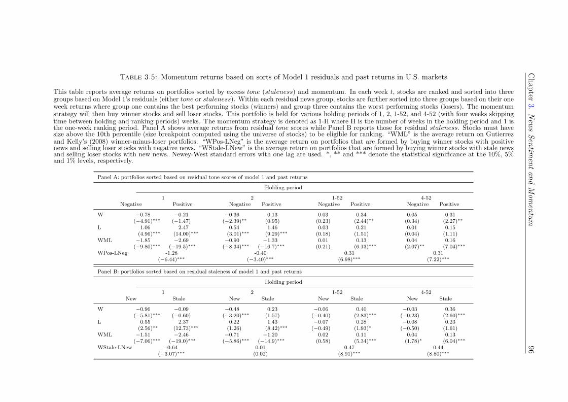
Chap
ter3.
New
sS
entim
ent
and
Mom
entu
m96
Table 3.5: Momentum returns based on sorts of Model 1 residuals and past returns in U.S. markets
This table reports average returns on portfolios sorted by excess tone (staleness) and momentum. In each week t, stocks are ranked and sorted into threegroups based on Model 1’s residuals (either tone or staleness). Within each residual news group, stocks are further sorted into three groups based on their oneweek returns where group one contains the best performing stocks (winners) and group three contains the worst performing stocks (losers). The momentumstrategy will then buy winner stocks and sell loser stocks. This portfolio is held for various holding periods of 1, 2, 1-52, and 4-52 (with four weeks skippingtime between holding and ranking periods) weeks. The momentum strategy is denoted as 1-H where H is the number of weeks in the holding period and 1 isthe one-week ranking period. Panel A shows average returns from residual tone scores while Panel B reports those for residual staleness. Stocks must havesize above the 10th percentile (size breakpoint computed using the universe of stocks) to be eligible for ranking. “WML” is the average return on Gutierrezand Kelly’s (2008) winner-minus-loser portfolios. “WPos-LNeg” is the average return on portfolios that are formed by buying winner stocks with positivenews and selling loser stocks with negative news. “WStale-LNew” is the average return on portfolios that are formed by buying winner stocks with stale newsand selling loser stocks with new news. Newey-West standard errors with one lag are used. *, ** and *** denote the statistical significance at the 10%, 5%and 1% levels, respectively.
Panel A: portfolios sorted based on residual tone scores of model 1 and past returns
Holding period
1 2 1-52 4-52Negative Positive Negative Positive Negative Positive Negative Positive
W −0.78 −0.21 −0.36 0.13 0.03 0.34 0.05 0.31(−4.91)∗∗∗ (−1.47) (−2.39)∗∗ (0.95) (0.23) (2.44)∗∗ (0.34) (2.27)∗∗
L 1.06 2.47 0.54 1.46 0.03 0.21 0.01 0.15(4.96)∗∗∗ (14.00)∗∗∗ (3.01)∗∗∗ (9.29)∗∗∗ (0.18) (1.51) (0.04) (1.11)
WML −1.85 −2.69 −0.90 −1.33 0.01 0.13 0.04 0.16(−9.80)∗∗∗ (−19.5)∗∗∗ (−8.34)∗∗∗ (−16.7)∗∗∗ (0.21) (6.13)∗∗∗ (2.07)∗∗ (7.04)∗∗∗
WPos-LNeg -1.28 -0.40 0.31 0.31(−6.44)∗∗∗ (−3.40)∗∗∗ (6.98)∗∗∗ (7.22)∗∗∗
Panel B: portfolios sorted based on residual staleness of model 1 and past returns
Holding period
1 2 1-52 4-52New Stale New Stale New Stale New Stale
W −0.96 −0.09 −0.48 0.23 −0.06 0.40 −0.03 0.36(−5.81)∗∗∗ (−0.60) (−3.20)∗∗∗ (1.57) (−0.40) (2.83)∗∗∗ (−0.23) (2.60)∗∗∗
L 0.55 2.37 0.22 1.43 −0.07 0.28 −0.08 0.23(2.56)∗∗ (12.73)∗∗∗ (1.26) (8.42)∗∗∗ (−0.49) (1.93)∗ (−0.50) (1.61)
WML −1.51 −2.46 −0.71 −1.20 0.02 0.11 0.04 0.13(−7.06)∗∗∗ (−19.0)∗∗∗ (−5.86)∗∗∗ (−14.9)∗∗∗ (0.58) (5.34)∗∗∗ (1.78)∗ (6.04)∗∗∗
WStale-LNew -0.64 0.01 0.47 0.44(−3.07)∗∗∗ (0.02) (8.91)∗∗∗ (8.80)∗∗∗

Chapter 3. News Sentiment and Momentum 97
The short-run reversal and longer-run momentum effects are consistent with the
mechanisms of both Tetlock (2011) and Hong and Stein (1999). For short-run
reversals, Tetlock (2011) models the interaction between rational and imperfectly
rational investors. Because rational investors know that irrational investors will
react to stale news, they will jump in and trade on the news first, causing the
particularly strong overreaction in the short run. In the longer run, the mecha-
nism of Hong and Stein (1999) can explain the underreaction to news that causes
momentum effects. Hong and Stein (1999) model the interaction between the news
watcher and the momentum trader who are both not fully rational. News watch-
ers trade on news only while momentum traders can only condition their trades
on historical prices. Moreover, not all news traders receive the news at the same
time (i.e., slow diffusion of news), which causes the underreaction to news among
news watchers. Momentum traders observe the trend created by news traders and
start trading aggressively on it. This interaction between the two groups causes
momentum effects in stock prices.
The findings in this subsection are based on separate examinations of news tone
and staleness. However, it makes sense to expect that negative news that has
been repeated a few times in the media should have a different impact on the
market than the new negative news. Given that investors overreact to stale news
and that they also overreact to positive news in the short run as I showed above,
I expect that they will overreact to stale positive news rather than new positive
news in the first few weeks of holding periods. I will test this hypothesis in the
next subsection.
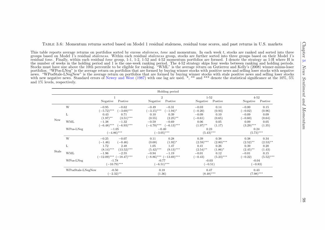
Chap
ter3.
New
sS
entim
ent
and
Mom
entu
m98
Table 3.6: Momentum returns sorted based on Model 1 residual staleness, residual tone scores, and past returns in U.S. markets
This table reports average returns on portfolios sorted by excess staleness, tone and momentum. In each week t, stocks are ranked and sorted into threegroups based on Model 1’s residual staleness. Within each residual staleness group, stocks are further sorted into three groups based on their Model 1’sresidual tone. Finally, within each residual tone group, 1-1, 1-2, 1-52 and 4-52 momentum portfolios are formed. I denote the strategy as 1-H where H isthe number of weeks in the holding period and 1 is the one-week ranking period. The 4-52 strategy skips four weeks between ranking and holding periods.Stocks must have size above the 10th percentile to be eligible for ranking. “WML” is the average return on Gutierrez and Kelly’s (2008) winner-minus-loserportfolios. “WPos-LNeg” is the average return on portfolios that are formed by buying winner stocks with positive news and selling loser stocks with negativenews. “WPosStale-LNegNew” is the average return on portfolios that are formed by buying winner stocks with stale positive news and selling loser stockswith new negative news. Standard errors of Newey and West (1987) with one lag are used. *, ** and *** denote the statistical significance at the 10%, 5%and 1% levels, respectively.
Holding period
1 2 1-52 4-52Negative Postive Negative Postive Negative Postive Negative Postive
New
W −0.95 −0.62 −0.49 −0.31 −0.03 0.14 −0.00 0.15(−5.72)∗∗∗ (−3.69)∗∗∗ (−3.15)∗∗∗ (−1.94)∗ (−0.20) (0.93) (−0.02) (0.96)
L 0.43 0.71 0.10 0.39 −0.09 0.10 −0.09 0.09(1.97)∗∗ (3.51)∗∗∗ (0.55) (2.25)∗∗ (−0.61) (0.65) (−0.60) (0.64)
WML −1.38 −1.32 −0.59 −0.69 0.06 0.05 0.09 0.05(−6.48)∗∗∗ (−6.93)∗∗∗ (−4.70)∗∗∗ (−6.13)∗∗∗ (1.97)∗∗ (1.17) (3.29)∗∗∗ (1.35)
WPos-LNeg −1.05 −0.40 0.23 0.24(−4.86)∗∗∗ (−3.05)∗∗∗ (5.43)∗∗∗ (5.73)∗∗∗
Stale
W −0.25 −0.07 0.11 0.28 0.39 0.38 0.38 0.34(−1.46) (−0.46) (0.68) (1.92)∗ (2.59)∗∗∗ (2.80)∗∗∗ (2.52)∗∗ (2.53)∗∗
L 1.72 2.48 1.05 1.47 0.41 0.26 0.39 0.20(8.14)∗∗∗ (13.52)∗∗∗ (5.42)∗∗∗ (9.13)∗∗∗ (2.54)∗∗ (1.86)∗ (2.45)∗∗ (1.43)
WML −1.96 −2.55 −0.94 −1.19 −0.01 0.12 −0.01 0.15(−12.09)∗∗∗ (−18.47)∗∗∗ (−8.86)∗∗∗ (−13.69)∗∗∗ (−0.43) (5.23)∗∗∗ (−0.22) (5.52)∗∗∗
WPos-LNeg -1.78 -0.77 -0.03 -0.04(−10.79)∗∗∗ (−6.51)∗∗∗ (−0.51) (−0.83)
WPosStale-LNegNew -0.50 0.18 0.47 0.43(−2.32)∗∗ (1.36) (8.48)∗∗∗ (7.98)∗∗∗

Chapter 3. News Sentiment and Momentum 99
3.4.4 Momentum portfolios sorted by staleness and tone
score
In this subsection, I provide the first joint examination of staleness and tone effects.
I first rank and sort stocks into three groups based on Model 1’s residual staleness,
and then within each staleness group I further sort stocks into three groups based
on their Model 1’s residual tone. Finally, I form 1-1, 1-2, 1-52 and 4-52 momentum
portfolios within each of the nine news groups, and results are reported in Table
3.6. Stocks with size below the 10th percentile at the end of the ranking period
are not ranked.
The upper half of Table 3.6 reports results in the new news groups. Apart from
the 1-1 portfolio where there is not much difference in the overreaction between
negative and positive news groups, investors generally still overreact more to pos-
itive news. The average momentum return on the 1-2 strategy is -0.69% per week
(t-statistic = -6.13), which is more negative than that in the negative news group
with -0.59% per week (t-statistic = -4.70).
In contrast to the results in Table 3.5 but consistent with Hong et al. (2000),
investors underreact to new negative news. The average return on the 4-52 port-
folio is 9bps per week (t-statistic = 3.29), which is higher than 5bps per week
(t-statistic 1.35, insignificant even at the 10% level) in the positive news group.
Thus, by taking into account another dimension of news namely staleness, I am
able to confirm the hypothesis of Hong et al. (2000) that investors underreact to
bad news. I add to their results that investors underreact to new bad news only.
Nevertheless, the difference in 4-52 WML returns between negative and positive
news groups is 4bps per week (not tabulated) with the insignificant associated
t-statistic of only 0.98. This difference for the 1-52 strategy is only 2bps per week
(t-statistic = 0.42). Thus, although the magnitude of the difference is consistent

Chapter 3. News Sentiment and Momentum 100
with Hong et al.’s (2000) hypothesis, momentum portfolios are not significantly
more profitable in the negative news group than in the positive news group.
The lower half of Table 3.6 shows results in the stale news group. In general,
investors overreact to stale positive news in the short run and underreact to stale
positive news in the long run. Within stale news groups, the 1-1 strategy earns
a negative average return of 2.55% per week (t-statistic = -18.47), which is much
more negative than -1.96% per week in the negative news group. In contrast to the
new news group, stocks with stale positive news exhibit much higher momentum
returns than those with stale negative news in the past week. The strategy yields
an average profit of 15bps per week (t-statistic = 5.52) among stocks with stale
positive news whereas it earns -1bp per week (t-statistic = -0.22) in the negative
stale news group.27
The difference in average 4-52 WML returns between negative and positive news
stocks is -0.16% per week (not tabulated) with the significant t-statistic of -3.46.
Therefore, the momentum strategy is significantly more profitable in the positive
news group than among negative news stocks. Finally, it should also be noted
again that, regardless of news tone and staleness, momentum portfolios being
conditioned on news yield higher average returns than the normal Gutierrez and
Kelly’s momentum strategies. These findings are consistent with Chan (2003) that
the momentum effect is driven by investors’ underreaction to news. I attempted to
reduce the bid-ask bounce that causes short-run reversals by using the midpoint
of bid and ask quotes to compute returns.
27In untabulated results, for the 1-1 strategy among stocks with negative news in the pastweek, the difference between the average WML return for the stale news group and that for thenew news group is -0.58% per week (t-statistic = -2.87, significant at the 1% level). Amongstocks with positive news, the difference is -1.23% per week with an associated t-statistic of-7.33, statistically significant at the 1% level. The higher difference for positive news suggeststhat markets overreact more to stale positive news in the short run.

Chapter 3. News Sentiment and Momentum 101
New trading strategies
Two interesting observations can be seen from Table 3.6. Firstly, the strategy
(WPos-LNeg) that buys positive news winners and sells negative news losers is
not profitable in the stale news group. The 1-52 WPos-LNeg strategy earns an
average return of -3bps per week (t-statistic = -0.51) in the stale news group while
it yields a significant profit of 23bps per week (t-statistic = 5.43) in the new news
group. This suggests that the profitability of trading strategies that sort stocks
based on news tone only is not robust to the joint examination both news features.
Secondly, a new trading strategy that seems to be more persistent is the one that
buys winner stocks with stale positive news in the past week and sells loser stocks
with new negative news over the same period (the last row of Table 3.6). As with
normal momentum strategies, this news strategy does not incur any look-ahead
bias because all information is available at the end of each ranking period. For
the 1-52 portfolio, this strategy earns an average return of 47bps per week, with
the t-statistic of 8.48, which is statistically significant at the 1% level. This 1-52
news momentum strategy earns 0.36% per week higher than the respective 1-52
Gutierrez and Kelly’s momentum portfolio. This difference is both economically
and statistically significant at the 1% level (t-statistic of the difference = 6.52,
not tabulated). Similarly, the 4-52 news momentum strategy also yields 0.32%
per week higher than the normal 4-52 momentum portfolio with a significant
associated t-statisitc of 6.07.
Since this news strategy produces economically and statistically significant returns
and also clearly represents market’s considerable underreaction to news, I will focus
on examining the robustness of this news strategy for the rest of the study. I will
use the term ‘news momentum’ and ‘WPosStale-LNegNew’ interchangeably to
represent my new trading strategy that exploits both staleness and tone of news.

Chapter 3. News Sentiment and Momentum 102
3.5 Sensitivities
In this section, I examine the sensitivity of my main results in Table 3.6 to several
variations from the baseline analysis. Firstly, I test whether the average return
on news momentum (WPosStale-LNegNew) portfolios is still significant after ad-
justing for risks using the Fama and French (1993) three-factor model. Secondly,
I examine whether the news momentum effect is a manifestation of Gutierrez and
Kelly (2008)’s weekly momentum effects or whether they are independent from
each other. Thirdly, I provide robustness tests for the news momentum effect us-
ing residuals from different variations to Model 1. Finally, I investigate whether
my findings are sensitive to the exclusion of penny stocks, the impact of size, the
use CRSP data, and downside risks. More importantly, the next section shows
that the profitability of news momentum strategies is robust to out-of-sample
tests, thereby avoiding the critique of “data-snooping” bias of Lo and MacKinlay
(1990a).
3.5.1 Risk-adjusted returns
Table 3.7 shows the properties of the normal unconditional WML portfolio and
WPosStale-LNegNew portfolios by regressing their weekly returns on the Fama
and French (1993) three-factor model (FF3F).28 In order to examine whether one
anomaly is a capture of the other, I also regress the WML return on the WPosStale-
LNegNew return and vice versa. If the news momentum portfolio (the right-
hand side variable) is stronger than the unconditional momentum portfolio (the
left-hand side variable), we should see the intercept from this regression to be
economically and statistically equal to zero.
28Fama and French’s risk factors are downloaded from Ken French’s website.

Chapter 3. News Sentiment and Momentum 103
Table 3.7: Risk-adjusted returns on news momentum portfolios in U.S. mar-kets
This table reports average risk-adjusted returns for unconditional momentum portfolios (whichare formed purely based on past returns as in Table 3.3) and news momentum portfolios whoseconstruction is described in Table 3.6). “FF3F” are returns on the Fama and French threefactors, which are obtained from Ken French’s website. “WML” is the weekly return on the rawGutierrez and Kelly’s (2008) winner-minus-loser portfolio (sorted based on past returns only).“WPosStale-LNegNew” is the average return on portfolios that are formed by buying winnerstocks with stale positive news and selling loser stocks with new negative news. If the LHS isWML then the RHS variable is the 4-52 News Momentum portfolio return. Alternatively, ifthe LHS is News WML then the RHS variable is the return on the 4-52 unconditional WMLportfolio. Stocks with size below the 10th percentile at the end of the ranking period are notranked. Newey-West standard errors with 1 lag are used. *, ** and *** denote the statisticalsignificance at the 10%, 5% and 1% levels, respectively.
Holding periodLHS RHS 1 2 1-52 4-52
WML FF3F −2.88 −1.49 0.06 0.11(−18.5)∗∗∗ (−16.6)∗∗∗ (2.75)∗∗∗ (6.01)∗∗∗
FF3F & WPosStale-LNegNew −2.97 −1.58 0.03 0.10(−16.3)∗∗∗ (−14.6)∗∗∗ (1.42) (4.63)∗∗∗
WPosStale-LNegNew FF3F −0.49 0.17 0.47 0.43(−2.32)∗∗ (1.31) (8.45)∗∗∗ (7.92)∗∗∗
FF3F & WML −0.66 0.07 0.42 0.39(−3.66)∗∗∗ (0.62) (8.71)∗∗∗ (7.90)∗∗∗
The upper half of Table 3.7 shows the intercept from the regression with WML
returns on the left-hand side. I drop stocks with size below the 10th percentile at
the end of each ranking period. The FF3F model cannot rationalize the weekly
momentum effect as the magnitude of all risk-adjusted returns almost stays the
same or even higher. The short-run reversal 1-1 and 1-2 strategies still incur the
loss of -2.88% and -1.49% per week respectively, which are even more negative
than the raw average return in Table 3.3. Risk-adjusted returns on 1-52 and 4-52
portfolios are still the same as their raw returns with 6bps (t-statistic = 2.75) and
11bps per week (t-statistic = 6.01) respectively, which are both economically and
statistically significant.
Adding the news momentum (WPosStale-LNegNew) return in the right-hand side
of the regression does not reduce the alpha in all strategies but the 1-52 strategy.
When I regress Gutierrez and Kelly’s (2008) 1-52 WML returns on the FF3F and
the WPosStale-LNegNew return, the intercept reduces to 3bps per week with an

Chapter 3. News Sentiment and Momentum 104
associated t-statistic of 1.42, which is both economically and statistically insignif-
icant. This low intercept indicates that my news momentum effects are stronger
than the 1-52 momentum effect of Gutierrez and Kelly (2008). Nevertheless, the
4-52 WML portfolio is still strong with the intercept being 10bps per week (t-
statistic = 4.63), which is statistically significant at the 1% level.
The lower half of Table 3.7 reports the intercept from regressions where the left-
hand side variable is returns on the WPosStale-LNegNew portfolio. The FF3F
model still cannot explain returns on the news momentum portfolio as all inter-
cepts are still as high as their raw returns. When I add the return on Gutierrez
and Kelly’s (2008) WML portfolios on the right-hand side of the regression, the
intercept in all strategies is still high and statistically significant although the
magnitude is slightly reduced. The intercept of 1-52 regression is 42bps per week
with an associated t-statistic of 8.71, which is economically and statistically sig-
nificant. Although the alpha of 4-52 portfolio in the four-factor model is 39bps
per week (t-statistic = 7.90), 4bps lower than that from the FF3F model, it is still
economically and statistically high.29
To sum up, Table 3.7 shows that my news momentum portfolios and Gutierrez and
Kelly’s (2008) unconditional momentum are independent from each other. For the
1-52 strategy, my news momentum portfolio is much stronger, and able to fully
capture the return on Gutierrez and Kelly’s (2008) momentum portfolios.
3.5.2 News residuals from Model 8 and Model 11
I repeat the exercise in Table 3.6, but use the residuals from Model 8, which
includes log(size), log(1 + analyst), book-to-market ratios, industry dummies,
29To be conservative, I use returns on Gutierrez and Kelly’s 4-52 momentum portfolios, whichare their strongest portfolios, in order to explain returns on my news momentum strategies.

Chapter 3. News Sentiment and Momentum 105
log(1+earn), and log(1+merger) as controlled variables. The two important con-
trols in this Model are earning news (earn) and merger news (merger). As noted
above, it may be the case that my results are driven by the effects of earnings
news (Tetlock et al., 2008) and merger news (Ahern and Sosyuara, 2013), which
also have return predictability. If returns on the news momentum portfolio be-
come insignificant and small by using residuals from Model 8, then my results
are not attributable to general firm-specific news, but instead capture the return
predictability from earnings news and the well-known stock return anomaly from
mergers and acquisition.
Table 3.8 shows that my results are still robust to earnings and merger news. In
fact, the news momentum effect is even stronger. The short-run reversal (1-1)
strategy disappears with the average return of -0.24% per week and an associated
t-statistic of -1.33, which is statistically insignificant even at the 10% level. The
WPosStale-LNegNew portfolio earns a significantly positive average return start-
ing from week two of holding periods. The 1-2 strategy yields an average return
of 29bps per week (t-statistic = 2.63). The best performing news portfolio is 1-52,
which earns an average return of 48bps per week (t-statistic = 7.74). In sum,
Table 3.8 indicates that my results are not driven by earnings and merger news.
The next robustness check is to use residuals from Model 11, which adds volatility
ranks (IV OL) in the model 8. Controlling for IV OL is motivated by Bandarchuk
and Hilscher (2013), who argue that when one sorts stocks based on firm charac-
teristics, they also pick up stocks with extreme total risks that make the newly
refined portfolio to earn higher returns. In other words, it is the total risk, not the
sorting characteristic employed by researchers, that drives the higher profit. Us-
ing residual analyst coverage (that controls for IV OL), Bandarchuk and Hilscher
(2013) find that Hong et al.’s (2000) results are not due to the effect of analyst
coverage but purely total risks. In similar spirits, I employ residuals from Model
11 and report results Table 3.9.

Chapter 3. News Sentiment and Momentum 106
However, as mentioned above, Model 11 suffers from potential endogeneity prob-
lems in that news can also determine volatility. Griffin et al. (2011) show that
volatility is much higher on news days than non-news days. Tetlock (2011) finds
that news staleness is associated with lower return volatility. Thus, to the extent
that news can affect volatility, using Model 11 will be conservative as I signifi-
cantly reduce the power of my tests by regressing tone (or staleness) on a noisy
proxy for itself, thereby biasing the residuals. Although I take this conservative
approach to control for IV OL, I can confirm that the news momentum strategy
remains profitable (but weaker). The 1-52 news strategy yields the average return
of 0.15% per week with the significant associated t-statistic of 2.15.
Table 3.9 shows that returns on the news momentum portfolios are weaker; but
the average return on the 1-52 WPosStale-LNegNew strategy, the most persistent
portfolio, is 0.15% per week (t=2.15) – still economically high and statistically
significant at the 5% level. The 1-1 news strategy incurs a significant reversal
in the first week of holding period with -0.60% per week (t=-4.57). Similar to
results in the previous tables, the news strategy stops reversing in week 2: the
1-2 news strategy yields an insignificant negative return of -0.12% per week with
an associated t-statistic of -1.43, insignificant even at the 10% level. Although
the 4-52 WPosStale-LNegNew portfolio earns an average return of 11bps per week
(t=1.65), the fact that the best performing strategy (1-52) still yields a signifi-
cantly positive average return indicates that my news momentum portfolios are
not just an artifact of extreme selection of stocks based on total risks.

Chap
ter3.
New
sS
entim
ent
and
Mom
entu
m107
Table 3.8: Momentum returns sorted based on Model 8 residual staleness, residual tone scores, and past returns in U.S. markets
This table reports average returns on portfolios sorted by excess staleness, tone and momentum. In each week t, stocks are ranked and sorted into threegroups based on Model 8’s residual staleness. Within each residual staleness group, stocks are further sorted into three groups based on their Model 8’sresidual tone. Finally, within each residual tone group, 1-1, 1-2, 1-52 and 4-52 momentum portfolios are formed. I denote the strategy as 1-H where H is thenumber of weeks in the holding period and 1 is the one-week ranking period. The 4-52 strategy skips four weeks between ranking and holding periods. Stocksmust have size above the 10th percentile to be eligible for ranking. “WML” is the average return on winner-minus-loser portfolios. “WPos-LNeg” is theaverage return on portfolios that are formed by buying winner stocks with positive news and selling loser stocks with negative news. “WPosStale-LNegNew” isthe average return on portfolios that are formed by buying winner stocks with stale positive news and selling loser stocks with new negative news. Newey-Weststandard errors with one lag are used. *, ** and *** denote the statistical significance at the 10%, 5% and 1% levels, respectively. The purpose of this tableis to show that the profitability of “WPosStale-LNegNew” portfolios is not a capture of earnings and merger news effects.
Holding period
1 2 1-52 4-52Negative Postive Negative Postive Negative Postive Negative Postive
New
W −0.87 −0.50 −0.50 −0.14 −0.03 0.21 0.00 0.19(−5.14)∗∗∗ (−3.07)∗∗∗ (−3.21)∗∗∗ (−0.84) (−0.17) (1.34) (0.01) (1.24)
L 0.09 0.96 −0.06 0.53 −0.04 0.03 −0.03 0.02(0.46) (4.51)∗∗∗ (−0.38) (3.02)∗∗∗ (−0.26) (0.21) (−0.19) (0.13)
WML −0.97 −1.45 −0.43 −0.66 0.01 0.18 0.03 0.17(−5.10)∗∗∗ (−7.43)∗∗∗ (−3.90)∗∗∗ (−5.31)∗∗∗ (0.38) (3.78)∗∗∗ (1.06) (3.74)∗∗∗
WPos-LNeg −0.59 −0.07 0.24 0.22(−3.19)∗∗∗ (−0.57) (5.63)∗∗∗ (5.09)∗∗∗
Stale
W −0.22 −0.15 0.08 0.23 0.47 0.44 0.47 0.41(−1.35) (−1.00) (0.50) (1.50) (3.03)∗∗∗ (2.99)∗∗∗ (2.98)∗∗∗ (2.77)∗∗∗
L 1.78 2.95 1.06 1.75 0.45 0.31 0.44 0.22(8.15)∗∗∗ (14.27)∗∗∗ (5.54)∗∗∗ (10.11)∗∗∗ (2.77)∗∗∗ (2.07)∗∗ (2.73)∗∗∗ (1.52)
WML −2.01 −3.10 −0.98 −1.53 0.03 0.14 0.03 0.19(−11.91)∗∗∗ (−18.83)∗∗∗ (−9.27)∗∗∗ (−15.97)∗∗∗ (0.71) (5.07)∗∗∗ (0.68) (6.59)∗∗∗
WPos-LNeg -1.93 -0.84 -0.01 -0.03(−11.23)∗∗∗ (−7.31)∗∗∗ (−0.07) (−0.44)
WPosStale-LNegNew -0.24 0.29 0.48 0.44(−1.33) (2.63)∗∗∗ (7.74)∗∗∗ (7.25)∗∗∗

Chap
ter3.
New
sS
entim
ent
and
Mom
entu
m108
Table 3.9: Momentum returns sorted based on Model 11 residual staleness, residual tone scores, and past returns in U.S. markets
This table reports average returns on portfolios sorted by excess staleness, tone and momentum. In each week t, stocks are ranked and sorted into threegroups based on Model 11’s residual staleness. Within each residual staleness group, stocks are further sorted into three groups based on their Model 11’sresidual tone. Finally, within each residual tone group, 1-1, 1-2, 1-52 and 4-52 momentum portfolios are formed. I denote the strategy as 1-H where H is thenumber of weeks in the holding period and 1 is the one-week ranking period. The 4-52 strategy skips four weeks between ranking and holding periods. Stocksmust have size above the 10th percentile to be eligible for ranking. “WML” is the average return on winner-minus-loser portfolios. “WPos-LNeg” is theaverage return on portfolios that are formed by buying winner stocks with positive news and selling loser stocks with negative news. “WPosStale-LNegNew” isthe average return on portfolios that are formed by buying winner stocks with stale positive news and selling loser stocks with new negative news. Newey-Weststandard errors with one lag are used. *, ** and *** denote the statistical significance at the 10%, 5% and 1% levels, respectively. The purpose of this tableis to show that the profitability of “WPosStale-LNegNew” portfolios is not a capture of earnings, merger news, and volatility effects.
Holding period
1 2 1-52 4-52Negative Postive Negative Postive Negative Postive Negative Postive
New
W −0.51 −0.52 −0.23 −0.14 0.13 0.29 0.14 0.26(−3.47)∗∗∗ (−3.09)∗∗∗ (−1.57) (−0.87) (0.87) (1.88)∗ (0.98) (1.68)∗
L 0.41 1.18 0.24 0.71 0.13 0.21 0.13 0.21(2.50)∗∗ (5.42)∗∗∗ (1.55) (4.14)∗∗∗ (0.88) (1.45) (0.91) (1.44)
WML −0.92 −1.71 −0.47 −0.85 −0.00 0.08 0.01 0.05(−7.81)∗∗∗ (−7.98)∗∗∗ (−6.31)∗∗∗ (−6.81)∗∗∗ (−0.00) (2.09)∗∗ (0.56) (1.34)
WPos-LNeg −0.93 −0.38 0.16 0.13(−6.45)∗∗∗ (−3.59)∗∗∗ (3.83)∗∗∗ (3.07)∗∗∗
Stale
W −0.24 −0.19 0.07 0.12 0.42 0.28 0.42 0.24(−1.41) (−1.26) (0.47) (0.81) (2.70)∗∗∗ (1.80)∗ (2.62)∗∗∗ (1.59)
L 1.76 3.18 1.05 1.79 0.43 0.10 0.41 −0.00(8.17)∗∗∗ (15.20)∗∗∗ (5.52)∗∗∗ (10.28)∗∗∗ (2.66)∗∗∗ (0.64) (2.56)∗∗ (−0.02)
WML −1.99 −3.37 −0.97 −1.67 −0.01 0.18 0.01 0.25(−12.23)∗∗∗ (−19.87)∗∗∗ (−9.34)∗∗∗ (−17.15)∗∗∗ (−0.08) (6.41)∗∗∗ (0.10) (8.30)∗∗∗
WPos-LNeg -1.95 -0.93 -0.15 -0.17(−11.58)∗∗∗ (−8.35)∗∗∗ (−2.36)∗∗ (−2.55)∗∗
WPosStale-LNegNew -0.60 -0.12 0.15 0.11(−4.57)∗∗∗ (−1.43) (2.15)∗∗ (1.65)

Chapter 3. News Sentiment and Momentum 109
The final point worth noticing again is that existing trading strategies in the
literature that are conditioned only on news tone (e.g., those of Sinha (2012),
which I denote WPos − LNeg portfolios) are not profitable among stocks with
stale news. My news momentum strategy overcomes this by conditioning the trade
on both news features. As I will show in the next section, my trading strategy also
works in 21 other developed markets whereas the profitability of existing strategies
is not robust to different degrees of staleness.
In sum, I do not find evidence to support Hong et al.’s (2000) hypothesis that “bad
news travels slowly” and causes momentum effects in stock returns. Using residuals
from Model 8 and Model 11, I find that even after I consider the dimension of
staleness, markets still underreact to positive news (the average momentum return
in the positive news group is significantly higher than that in the negative news
group). In other words, even though I could confirm Hong et al.’s (2000) hypothesis
using Model 1, the finding is not robust to considerations of earnings, merger news,
and IV OL. I again support the original theory of Hong and Stein (1999) that
momentum returns are driven by underreaction in prices to (positive) news.
More untabulated robustness checks
Penny stocks With the exclusion of stocks priced below $5 at the end of each
ranking period, I confirm that my results do not qualitatively change. For ex-
ample, using Model 8’s residuals, the 1-52 news momentum portfolio still earns a
significant average return of 0.24% per week with an associated t-statistic of 4.56,
statistically significant at the 1% level. Thus, my findings are not driven by penny
stocks.
Size I re-examine the profitability of news momentum portfolios by dropping all
stocks with size below the median at the end of each ranking period. Using Model

Chapter 3. News Sentiment and Momentum 110
8, the average returns on 1-52 and 4-52 strategies are 0.27% (t-statistic = 7.20)
and 0.26% (t-statistic = 7.17) per week, respectively. These results show that the
profitability of news strategies is robust to the exclusion of small stocks.30
CRSP’s daily data In more untabulated results, I repeat the exercise in Table
3.6 using daily data from the Center for Research in Security Prices (CRSP)
instead of midpoint returns from TRTH. I also confirm that my results do not
qualitatively change. For example, with Model 8’s residuals, the average returns
on 1-52 and 4-52 news momentum (WPosStale-LNegNew) portfolios are 0.11%
(t-statistic = 4.01) and 0.10% per week (t-statistic = 3.91) respectively, which are
economically and statistically significant at the 1% level. I report midpoint returns
to be consistent with Gutierrez and Kelly (2008) who argue that this method can
alleviate the bid-ask bounce effect in calculating portfolio returns.
Downside risks: I also test the business cycle dependence of my news momen-
tum portfolios. Garcia (2013) shows that news sentiment has strong predictabil-
ity during recessions as dated by the NBER.31 Consequently, I am interested in
whether the average profit of news momentum strategies is stronger during reces-
sions. The disadvantage of this test is that my sample period is short (between
January 2003 and December 2011), leaving me with only one recession period from
December 2007 to June 2009 (or 87 weeks). Thus, because I have unequal periods
of expansions and recessions, my tests are weakened and I can only interpret the
magnitude of returns and the percentage of weeks having negative returns. Us-
ing residuals from Model 8, I can report that average returns on the 1-52 news
momentum portfolio are 0.51% per week (t-statistic = 2.75) and 0.46% per week
30My results are stronger with Model 11’s residuals in the sample of large stocks. With theresiduals from Model 11, the 1-52 and 4-52 news strategies on average yield 25bps per week withan associated t-statistic above 6.97, which is economically and statistically significant at the 1%level. This finding indicates that the weaker average return on news momentum portfolios usingModel 11’s residuals is due to the returns (and high volatility) of small stocks.
31Grundy and Martin (2001) and Daniel and Moskowitz (2011) find that betas of monthlymomentum portfolios are lower following down markets.

Chapter 3. News Sentiment and Momentum 111
(t-statistic = 7.20) during contractions and expansions, respectively. These returns
are both economically and statistically significant at the 1% level. The average re-
turn during contractions is only 5bps higher than that during expansionary times.
Finally, the 1-52 news strategy earns negative returns in 36.78% of the (87) re-
cession weeks whereas 33.96% of the (371) expansion weeks has negative returns.
For comparison purposes, the Gutierrez and Kelly’s (2008) 1-52 momentum port-
folio yields negative returns in 58.62% of the recession weeks while 29.92% of the
expansion weeks is negative. In other words, the news momentum strategy is less
exposed to recessions (or downside risks) than the normal momentum portfolio.
3.6 Out-of-sample evidence: International weekly
momentum returns
One disadvantage of using TRNA data is the relatively short period of time al-
though I employ weekly data, which gives me 458 weeks of returns. One way to
overcome this disadvantage is to use the TRNA’s international coverage, which
allows me to test the above findings with out-of-sample evidence. In fact, the re-
sults reported in previous sections, especially the profitability of news momentum
strategies, are not only true in the U.S., but they also hold in 21 other developed
markets. In this section, I essentially repeat the exercise in the previous section,
particularly Table 3.9, for 21 international markets. By doing so, I also provide
the first international study that links firms’ news to weekly momentum returns.
3.6.1 Data and weekly momentum returns
I employ TRTH again to collect daily market data for 21 developed markets.
Firms must be covered in TRNA to be included in the analysis. I repeat the data

Chapter 3. News Sentiment and Momentum 112
cleaning process as for the U.S. markets to get weekly data from Wednesday to
Wednesday, except that I do not use the midpoint of bid and ask quotes to calculate
returns. Rather, I compute weekly returns using closing prices from Wednesday
to Wednesday. The reason why I do not use midpoints of bid and ask prices
is because international markets generally do not have a specialist to facilitate
transactions as in the NYSE. Consequently, returns computed using midpoints
may not be tradeable.32
I follow Fama and French (2012) and categorize stocks into three regions: (i)
Japan; (ii) Asia Pacific, including Australia, New Zealand, Hong Kong and Singa-
pore (but not Japan); and finally (iii) Europe, including Austria, Belgium, Den-
mark, Finland, France, Germany, Greece, Ireland, Italy, the Netherlands, Norway,
Portugal, Spain, Sweden, Switzerland, and the United Kingdom. The purpose of
these market combinations is parsimony as well as maintaining a certain degree
of market integration. Most European countries are members of the European
Union (EU), which undoubtedly enjoy the benefits of market integration in the
Euro zone. As noted in Fama and French (2012), the most segmented region is
Asia Pacific, which may reduce the power of my portfolio tests. Appendix 3.A
reports summary statistics for these markets.
Table 3.10 reports raw momentum returns in each of the regions. The left-hand
side panel reports results using all stocks while the right-hand side panel drops
stocks with size below the 10th percentile (computed using the regional break-
point). Using the universe of stocks in each region, there is no evidence of mo-
mentum effect anywhere. The weekly momentum strategy of Gutierrez and Kelly
(2008) earns negative average returns for all strategies but the 4-52; but the 4-52
strategy is also economically and statistically insignificant in all markets.
32As TRTH also provides bid and ask prices, I am able to calculate returns with midpoint ofbid and ask prices. I confirm that my conclusions in international markets still hold.

Chap
ter3.
New
sS
entim
ent
and
Mom
entu
m113
Table 3.10: Summary statistics for weekly momentum portfolios between 19 February 2003 to 28 December 2011
This table reports average returns on Gutierrez and Kelly’s (2008) weekly momentum portfolios in international markets. In each week t, stocks are rankedand sorted into three groups based on their past one week returns where group one contains the best performing stocks (winners) and group three contains theworst performing stocks (losers). The momentum strategy will then buy winner stocks and sell loser stocks. This portfolio is held for various holding periodsof 1, 2, 3, 1-52, and 4-52 (with four weeks skipping time between holding and ranking periods) weeks. I denote the strategy as 1-H where H is the number ofweeks in the holding period and 1 is the one-week ranking period. Panel A reports results using all stocks while Panel B shows average returns on portfoliosthat do not rank stocks with size below the 10th percentile at the end of ranking periods. Microcaps are defined as stocks with market capitalization in thebottom 10% of the sample each week. “WML” is the average return on winner-minus-loser portfolios. Newey-West standard errors with one lag are used. *,** and *** denote the statistical significance at the 10%, 5% and 1% levels, respectively. The number of weeks in each sample is 463 weeks for Europe, 461for Japan, and 463 weeks for Asia. On average, the numbers of stocks in each winner or loser portfolio in Europe, Japan, and Asia are 1079, 690, and 619stocks per week, respectively.
Panel A: All Stocks Panel B: Excluding Microcaps
Holding period1 2 3 1-52 4-52 1 2 3 1-52 4-52
EuropeW −0.05 0.29 0.42 0.70 0.72 0.00 0.28 0.39 0.63 0.65
(−0.34) (2.00)∗∗ (2.96)∗∗∗ (4.87)∗∗∗ (5.01)∗∗∗ (0.02) (1.93)∗ (2.77)∗∗∗ (4.40)∗∗∗ (4.52)∗∗∗
L 1.92 1.36 1.15 0.72 0.70 1.49 1.08 0.93 0.63 0.61(11.83)∗∗∗ (8.67)∗∗∗ (7.35)∗∗∗ (4.87)∗∗∗ (4.70)∗∗∗ (9.20)∗∗∗ (6.95)∗∗∗ (5.98)∗∗∗ (4.24)∗∗∗ (4.11)∗∗∗
WML −1.97 −1.07 −0.72 −0.03 0.02 −1.48 −0.80 −0.54 0.00 0.04(−24.1)∗∗∗ (−19.1)∗∗∗ (−16.7)∗∗∗ (−1.69)∗ (1.48) (−19.3)∗∗∗ (−15.1)∗∗∗ (−12.8)∗∗∗ (0.02) (2.57)∗∗
JapanW −0.08 0.21 0.36 0.62 0.64 −0.09 0.15 0.28 0.50 0.52
(−0.57) (1.53) (2.57)∗∗ (4.24)∗∗∗ (4.35)∗∗∗ (−0.66) (1.12) (2.06)∗∗ (3.57)∗∗∗ (3.66)∗∗∗
L 1.56 1.15 0.98 0.66 0.65 0.83 0.69 0.61 0.48 0.47(8.43)∗∗∗ (6.74)∗∗∗ (5.90)∗∗∗ (4.33)∗∗∗ (4.20)∗∗∗ (5.03)∗∗∗ (4.40)∗∗∗ (3.98)∗∗∗ (3.31)∗∗∗ (3.27)∗∗∗
WML −1.63 −0.94 −0.62 −0.04 −0.01 −0.92 −0.54 −0.34 0.02 0.04(−13.8)∗∗∗ (−12.0)∗∗∗ (−10.9)∗∗∗ (−2.70)∗∗∗ (−0.06) (−9.45)∗∗∗ (−8.25)∗∗∗ (−7.13)∗∗∗ (1.41) (3.11)∗∗∗
Asia (ex. Japan)W −0.19 0.29 0.50 0.83 0.85 −0.23 0.20 0.40 0.71 0.73
(−1.02) (1.58) (2.75)∗∗∗ (4.63)∗∗∗ (4.73)∗∗∗ (−1.26) (1.15) (2.23)∗∗ (4.04)∗∗∗ (4.16)∗∗∗
L 2.29 1.69 1.43 0.90 0.86 1.45 1.12 0.97 0.70 0.68(10.87)∗∗∗ (8.38)∗∗∗ (7.17)∗∗∗ (4.78)∗∗∗ (4.61)∗∗∗ (7.36)∗∗∗ (5.77)∗∗∗ (5.02)∗∗∗ (3.84)∗∗∗ (3.77)∗∗∗
WML −2.48 −1.41 −0.93 −0.06 −0.01 −1.68 −0.91 −0.57 0.01 0.05(−20.1)∗∗∗ (−17.1)∗∗∗ (−14.7)∗∗∗ (−3.93)∗∗∗ (−0.17) (−16.5)∗∗∗ (−12.7)∗∗∗ (−10.1)∗∗∗ (0.80) (3.88)∗∗∗

Chapter 3. News Sentiment and Momentum 114
After dropping microcap stocks at the end of each ranking period, momentum
returns are higher although the 1-52 strategy is still not profitable. The 1-1 port-
folio produces average returns of -1.48%, -0.92% and -1.68% per week in Europe,
Japan and Asia, respectively. The average profit of the 1-52 strategy is almost zero
everywhere. The best performing portfolio is the 4-52 with four week skipping pe-
riod between ranking and holding periods. This strategy is profitable everywhere,
earning 4bps per week (t-statistic = 2.57) in Europe, 4bps per week (t-statistic
= 3.11) in Japan, and 5bps per week (t-statistic = 3.88) in Asia, which are all
statistically significant at least at the 5% level. Since the momentum effect is weak
in the presence of extremely small stocks and since these stocks are highly illiquid,
I will focus my analysis on the more investible strategy that drops these microcap
stocks at the end of each ranking period.
3.6.2 Momentum portfolios sorted by staleness and tone
Table 3.11 reports momentum returns sorted first by residual staleness and then
residual tone scores. Again, I use residuals from Model 11, which avoids the
critique of Bandarchuk and Hilscher (2013). This model choice is conservative not
only because of the endogeneity problem that weakens my tests, but also because
my U.S. results show that the profitability of news momentum portfolios is the
weakest (but still profitable) under this model. Nevertheless, I find that the news
momentum strategy earns significantly positive returns in all markets (even though
Gutierrez and Kelly’s (2008) 1-52 weekly momentum portfolio is not profitable).
I also use residuals from other models, and can confirm that my results do not
qualitatively change.
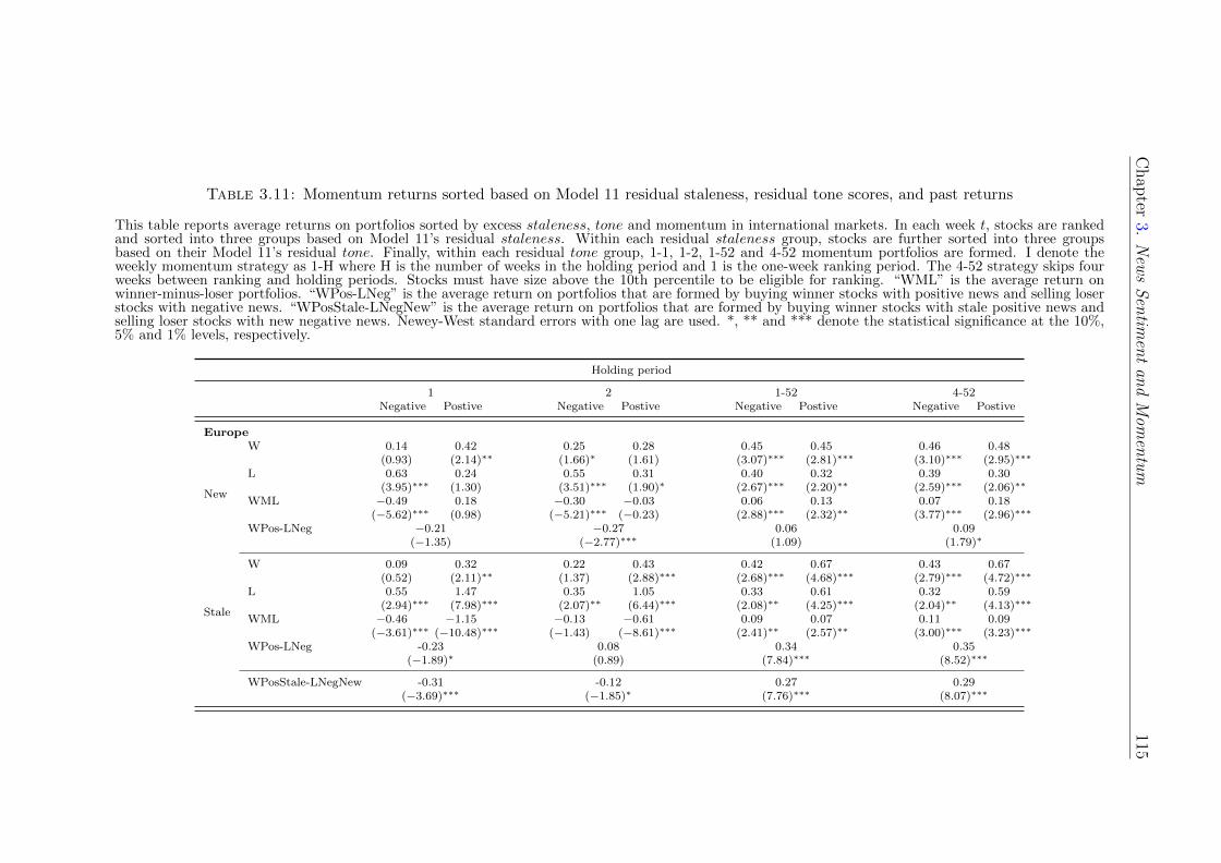
Chap
ter3.
New
sS
entim
ent
and
Mom
entu
m115
Table 3.11: Momentum returns sorted based on Model 11 residual staleness, residual tone scores, and past returns
This table reports average returns on portfolios sorted by excess staleness, tone and momentum in international markets. In each week t, stocks are rankedand sorted into three groups based on Model 11’s residual staleness. Within each residual staleness group, stocks are further sorted into three groupsbased on their Model 11’s residual tone. Finally, within each residual tone group, 1-1, 1-2, 1-52 and 4-52 momentum portfolios are formed. I denote theweekly momentum strategy as 1-H where H is the number of weeks in the holding period and 1 is the one-week ranking period. The 4-52 strategy skips fourweeks between ranking and holding periods. Stocks must have size above the 10th percentile to be eligible for ranking. “WML” is the average return onwinner-minus-loser portfolios. “WPos-LNeg” is the average return on portfolios that are formed by buying winner stocks with positive news and selling loserstocks with negative news. “WPosStale-LNegNew” is the average return on portfolios that are formed by buying winner stocks with stale positive news andselling loser stocks with new negative news. Newey-West standard errors with one lag are used. *, ** and *** denote the statistical significance at the 10%,5% and 1% levels, respectively.
Holding period
1 2 1-52 4-52Negative Postive Negative Postive Negative Postive Negative Postive
Europe
New
W 0.14 0.42 0.25 0.28 0.45 0.45 0.46 0.48(0.93) (2.14)∗∗ (1.66)∗ (1.61) (3.07)∗∗∗ (2.81)∗∗∗ (3.10)∗∗∗ (2.95)∗∗∗
L 0.63 0.24 0.55 0.31 0.40 0.32 0.39 0.30(3.95)∗∗∗ (1.30) (3.51)∗∗∗ (1.90)∗ (2.67)∗∗∗ (2.20)∗∗ (2.59)∗∗∗ (2.06)∗∗
WML −0.49 0.18 −0.30 −0.03 0.06 0.13 0.07 0.18(−5.62)∗∗∗ (0.98) (−5.21)∗∗∗ (−0.23) (2.88)∗∗∗ (2.32)∗∗ (3.77)∗∗∗ (2.96)∗∗∗
WPos-LNeg −0.21 −0.27 0.06 0.09(−1.35) (−2.77)∗∗∗ (1.09) (1.79)∗
Stale
W 0.09 0.32 0.22 0.43 0.42 0.67 0.43 0.67(0.52) (2.11)∗∗ (1.37) (2.88)∗∗∗ (2.68)∗∗∗ (4.68)∗∗∗ (2.79)∗∗∗ (4.72)∗∗∗
L 0.55 1.47 0.35 1.05 0.33 0.61 0.32 0.59(2.94)∗∗∗ (7.98)∗∗∗ (2.07)∗∗ (6.44)∗∗∗ (2.08)∗∗ (4.25)∗∗∗ (2.04)∗∗ (4.13)∗∗∗
WML −0.46 −1.15 −0.13 −0.61 0.09 0.07 0.11 0.09(−3.61)∗∗∗ (−10.48)∗∗∗ (−1.43) (−8.61)∗∗∗ (2.41)∗∗ (2.57)∗∗ (3.00)∗∗∗ (3.23)∗∗∗
WPos-LNeg -0.23 0.08 0.34 0.35(−1.89)∗ (0.89) (7.84)∗∗∗ (8.52)∗∗∗
WPosStale-LNegNew -0.31 -0.12 0.27 0.29(−3.69)∗∗∗ (−1.85)∗ (7.76)∗∗∗ (8.07)∗∗∗

Chap
ter3.
New
sS
entim
ent
and
Mom
entu
m116
Table 3.11 continued.
Holding period
1 2 1-52 4-52Negative Postive Negative Postive Negative Postive Negative Postive
Japan
New
W −0.01 −0.08 0.14 0.16 0.40 0.53 0.40 0.53(−0.08) (−0.42) (1.01) (0.98) (2.74)∗∗∗ (3.47)∗∗∗ (2.71)∗∗∗ (3.52)∗∗∗
L 0.39 0.82 0.41 0.63 0.31 0.36 0.31 0.38(2.58)∗∗∗ (3.64)∗∗∗ (2.88)∗∗∗ (3.39)∗∗∗ (2.30)∗∗ (2.59)∗∗∗ (2.35)∗∗ (2.69)∗∗∗
WML −0.40 −0.90 −0.27 −0.47 0.09 0.17 0.08 0.16(−4.14)∗∗∗ (−4.34)∗∗∗ (−3.75)∗∗∗ (−3.52)∗∗∗ (3.58)∗∗∗ (3.97)∗∗∗ (3.20)∗∗∗ (3.72)∗∗∗
WPos-LNeg −0.47 −0.26 0.22 0.22(−3.19)∗∗∗ (−2.33)∗∗ (5.45)∗∗∗ (5.51)∗∗∗
Stale
W 0.30 0.43 0.52 0.51 0.67 0.81 0.65 0.79(2.03)∗∗ (3.17)∗∗∗ (3.58)∗∗∗ (3.60)∗∗∗ (4.65)∗∗∗ (5.84)∗∗∗ (4.47)∗∗∗ (5.71)∗∗∗
L 0.55 1.30 0.59 1.00 0.47 0.65 0.47 0.62(3.27)∗∗∗ (7.57)∗∗∗ (3.90)∗∗∗ (6.25)∗∗∗ (3.52)∗∗∗ (5.23)∗∗∗ (3.50)∗∗∗ (5.01)∗∗∗
WML −0.25 −0.87 −0.07 −0.49 0.20 0.16 0.18 0.17(−2.08)∗∗ (−6.94)∗∗∗ (−0.71) (−5.26)∗∗∗ (5.68)∗∗∗ (5.01)∗∗∗ (4.95)∗∗∗ (5.50)∗∗∗
WPos-LNeg -0.12 -0.07 0.34 0.32(−1.01) (−0.84) (8.88)∗∗∗ (8.09)∗∗∗
WPosStale-LNegNew 0.04 0.10 0.50 0.47(0.33) (1.16) (8.77)∗∗∗ (8.40)∗∗∗
Asia (ex. Japan)
New
W 0.01 0.28 0.25 0.30 0.59 0.55 0.58 0.57(0.07) (1.01) (1.25) (1.38) (3.13)∗∗∗ (2.79)∗∗∗ (3.10)∗∗∗ (2.87)∗∗∗
L 0.86 1.04 0.78 0.94 0.44 0.47 0.46 0.46(3.52)∗∗∗ (4.00)∗∗∗ (3.47)∗∗∗ (3.90)∗∗∗ (2.37)∗∗ (2.54)∗∗ (2.49)∗∗ (2.51)∗∗
WML −0.84 −0.76 −0.53 −0.63 0.15 0.07 0.12 0.10(−5.35)∗∗∗ (−3.06)∗∗∗ (−4.43)∗∗∗ (−3.81)∗∗∗ (3.83)∗∗∗ (1.40) (3.18)∗∗∗ (1.81)∗
WPos-LNeg −0.58 −0.48 0.11 0.10(−2.45)∗∗ (−2.88)∗∗∗ (1.95)∗ (1.74)∗
Stale
W 0.35 0.40 0.40 0.66 0.90 1.10 0.89 1.06(1.52) (1.84)∗ (1.92)∗ (3.28)∗∗∗ (5.04)∗∗∗ (6.19)∗∗∗ (4.99)∗∗∗ (5.96)∗∗∗
L 1.29 1.31 0.74 1.05 0.77 0.91 0.75 0.92(5.08)∗∗∗ (5.87)∗∗∗ (3.75)∗∗∗ (4.98)∗∗∗ (4.54)∗∗∗ (5.22)∗∗∗ (4.45)∗∗∗ (5.23)∗∗∗
WML −0.94 −0.91 −0.34 −0.39 0.13 0.19 0.14 0.15(−3.67)∗∗∗ (−5.22)∗∗∗ (−2.09)∗∗ (−2.80)∗∗∗ (2.05)∗∗ (3.01)∗∗∗ (2.09)∗∗ (2.23)∗∗
WPos-LNeg -0.90 -0.08 0.34 0.31(−3.66)∗∗∗ (−0.49) (4.33)∗∗∗ (4.00)∗∗∗
WPosStale-LNegNew -0.46 -0.12 0.66 0.60(−2.62)∗∗∗ (−0.80) (7.93)∗∗∗ (7.32)∗∗∗

Chapter 3. News Sentiment and Momentum 117
Europe The first panel of Table 3.11 shows average news momentum returns for
different strategies in Europe (the last row). The WPosStale-LNegNew portfolio
still produces negative average return of -0.31% per week (t-statistic = -3.69) in
the first week of holding period. The average news momentum return increases to
27% per week (t-statistic = 7.76) for the 1-52 strategy, which is economically and
statistically significant. Recall that the average return on Gutierrez and Kelly’s
(2008) 1-52 momentum portfolios is almost zero in Table 3.10. Thus, my news
momentum portfolio is much stronger and not a confounding effect of their weekly
momentum counterpart. The 4-52 news strategy (with four-week skipping period)
yields the highest average return of 29bps per week with an associated t-statistic
of 8.07 – statistically significant at the 1% level. This average return is also higher
than the normal weekly momentum return in Table 3.10.
I find mixed evidence for Hong et al.’s (2000) hypothesis in Europe. Among
stocks with new news, the average momentum profit in positive news groups is
doubled that in negative news groups. The 4-52 momentum strategy yields an
average return of 18bps per week in the positive news group, which is 11bps
(untabulated t-statistic for this difference = 1.65, significant at the 10% level)
higher than that in the negative news group. This finding does not support Hong
et al. (2000), but is consistent with the U.S. evidence that underreaction to positive
news drives momentum returns. In contrast, I find supporting evidence for Hong
et al.’s (2000) hypothesis within the stale news group although the difference in
returns between positive news groups and negative news groups is only 2bps per
week and statistically insignificant. For example, the average momentum profit
on the 4-52 portfolio in the negative news group is 11bps per week, which is 2bps
higher than the average momentum return among stocks with good news, and an
associated t-statistic for this difference is only 0.57 (not tabulated). Consequently,
although these findings provide equivocal supports for Hong et al.’s hypothesis,
underreaction to positive news seems to be a stronger driver of momentum profits

Chapter 3. News Sentiment and Momentum 118
in both new and stale news groups. The final point of interest is that European
markets overreact to stale positive news, but not new positive news. The average
profit for 1-1 strategy among stale positive news stocks is -1.15% per week (t-
statistic = -10.48) while the average profit in the new positive news group is
0.18% per week (t-statistic = 0.98).
Japan The middle panel of Table 3.11 reports results for Japan. Surprisingly, the
news momentum strategy (reported in the last row) is highly profitable in Japan,
and more importantly it does not reverse in the first week. The average return on
the 1-1 WPosStale-LNegNew portfolio is 4bps per week (t-statistic = 0.33), which
is not significant in both economic and statistical terms. This evidence is important
because it is well known that the monthly momentum effect of Jegadeesh and
Titman (1993) is not present in Japan. I have shown that Gutierrez and Kelly’s
weekly momentum portfolios have significant reversals in the first few weeks of
holding periods. Consequently, my results shed lights on a new anomaly that is
very strong and persistent in a market that the known momentum strategies do not
“work”. Also in contrast to the normal Gutierrez and Kelly’s (2008) momentum
evidence in Table 3.10, the 1-52 news momentum strategy earns the highest return
in Japan with 50bps per week and an associated t-statistic of 8.77, statistically
significant at the 1% level. The 4-52 news strategy also performs well, yielding
47bps per week (t=8.40).
In testing Hong et al.’s (2000) hypothesis, Japan’s findings are consistent with
the European evidence that the momentum effect is marginally stronger among
stocks with stale negative news but much weaker in the new negative news group.
For example, within stale news groups, the 1-52 strategy in the negative news
group earns an average return 20bps per week (t-statistic = 5.68), which is only
4bps (t-statistic difference = 0.92) higher than that in the positive news group.
This supports the hypothesis, though weakly, that bad stale news travels slowly.

Chapter 3. News Sentiment and Momentum 119
But this slow diffusion of bad news is not found in the new news group where
the difference in profitability between two tone news groups is bigger. The 4-52
momentum portfolio earns 16bps per week (t-statistic = 3.72) among stocks with
positive news, which is doubled that in the bad news group. The difference of
8bps has the significant associated t-statistic of 1.96. Thus, as in Europe, the
underreaction to positive news is still a stronger driver of momentum returns in
Japan.
Finally, in terms of short-run overreaction, Japanese markets tend to overreact
to new news more than to stale news – in contrast to Tetlock (2011) – although
the difference is economically small. Within the new news group of stocks, the 1-1
strategy earns -0.40% (t-statistic = -4.14) and -0.90% per week (t-statistic = -4.34)
in the negative and positive news groups, respectively. These average returns are
more negative than the average returns of -0.25% and -0.87% per week for stale
negative and stale positive news groups, respectively.
Asia (ex. Japan) The last panel of Table 3.11 presents results for Asian mar-
kets. The 1-52 news momentum strategy is again the best, earning 0.66% per
week with an associated t-statistic of 7.93, statistically significant at the 1% level.
This news momentum effect is obviously not a manifestation of the normal mo-
mentum effect because the Gutierrez and Kelly’s (2008) 1-52 momentum strategy
earns only 0.01% per week (t-statistic = 0.80) in Asia. The 4-52 news portfolio
yields the slightly lower return of 60bps per week (t-statistic = 7.32), which is
still higher than that in other markets. Among all markets, the news momentum
strategy performs the best in Asia.
I also find very weak supporting evidence for Hong et al.’s (2000) hypothesis that
“bad news travels slowly” in Asia because the difference in WML returns between
negative and positive news groups is not significant. Also, in contrast to Europe
and Japan, this support is in the new news group only. Within new news groups,

Chapter 3. News Sentiment and Momentum 120
the 1-52 momentum portfolio formed using stocks with negative news earns 15bps
per week (t-statistic = 3.83), compared with 7bps per week among positive news
stocks. This 8bps difference is however not statistically significant (t-statistic =
1.32, not tabulated). Looking at stale news groups, although the average WML in
the positive news group is higher than in the negative news group, the difference
is again both economically and statistically insignificant.
To sum up, this subsection has shown that my news momentum strategy that buys
winner stocks with stale positive news in the past one week and sells loser stocks
with new negative news over the same period yields profitable returns everywhere
for the holding period of up to 52 weeks. This significant profitability is only iden-
tifiable by simultaneously investigating both staleness and tone of news. Unlike
the well-known monthly momentum portfolio and weekly momentum strategies,
this news momentum portfolio is even highly profitable and not reversing in the
first week of holding period in Japan. Finally, unlike the U.S. evidence where the
rejection of Hong et al.’s (2000) hypothesis is very strong, the rejection is weak in
Europe, Japan, and the rest of Asia. In most cases the difference in momentum
returns between negative and positive news groups is not statistically significant
and is dependent on the degree of staleness of news, not just the tone of news.
Nevertheless, regardless of the tone and staleness of news, I still find strong empir-
ical evidence for the original model of Hong and Stein (1999) that underreaction
to news is the driver of momentum returns. In all markets, momentum strate-
gies that are conditioned on news yield higher average returns than the normal
momentum portfolio of Gutierrez and Kelly (2008).
3.7 Conclusion
The main contribution of this study is, with a much bigger and more current
news dataset, to jointly investigate the effect of tone and staleness of news on

Chapter 3. News Sentiment and Momentum 121
weekly momentum returns. In the U.S. markets, I do not find evidence to support
Hong et al.’s (2000) hypothesis that momentum returns are driven by the slow
diffusion of bad news. Instead, I find that it is the underreaction to positive news
that drives the profitability of momentum portfolios. However, using international
data from 21 developed markets, I find that both bad news and good news can
drive momentum returns. Nevertheless, regardless of the tone and staleness of
news, I provide strong evidence for Hong and Stein’s (1999) theoretical model
that momentum effects are attributable to the market’s underreaction to news in
general. Finally, I document a new investible trading strategy that buys winner
stocks with stale positive news in the ranking period and sells losers with new
negative news over the same period. This strategy is highly profitable everywhere
including Japan where the normal momentum strategy does not work. These
findings, which have not been documented in the literature, can only be found
by jointly examining the two features of news. My results are important because
they provide strong empirical support (both in the U.S. and international markets)
for behavioral theories, specifically the underreaction to news of Hong and Stein
(1999), which is rare to find. The fact that my news momentum strategy is
profitable in all markets suggests that investors everywhere have similar behavioral
bias and underreact to news.
3.A Appendix: Summary statistics for Europe,
Japan, and Asia (ex. Japan)
As mentioned in the body text, I source international market data from TRTH’s
daily database. This database is fully compatible with TRNA via the Reuters
Identification Code (RIC), which is used to match stocks’ market data with news
between the two databases. Following Griffin et al. (2011), Fama and French
(2012) and the vast majority of international studies, all returns are calculated in

Chapter 3. News Sentiment and Momentum 122
U.S. dollar terms and weekly returns are set to missing if they are greater than
300% and reversed in the following week. Specifically, if either rt or rt−1 is greater
than 300% and (1 + rt−1)(1 + rt)− 1 ≤ 50%, then both rt−1 and rt are treated as
missing values. I use international book values of equity from WorldScope (data
item: WC05476). The book-to-market ratio is then computed by dividing book
value of equity by the market price of the stock. Exchange rates are provided by
TRTH. Similar to the U.S. study, I obtain weekly analyst coverage (defined as
the number of analysts who provide fiscal year one earnings estimates in the past
quarter) from I/B/E/S.
Table 3.A.1 reports summary statistics for each region. Consistent with previous
international studies (e.g., Fama and French (2012)) Europe has the highest num-
ber of stocks in three regions. The lowest numbers of stocks for Europe, Japan,
and Asia (ex. Japan) are 2,633, 1920, and 1420 stocks, respectively in 2003. The
largest numbers of stocks are 4,556 stocks for Europe in 2009, 2,734 stocks for
Japan in 2011, and 2,508 stocks for Asia in 2010. Due to its market size, Europe
also has the highest total number of news articles with over 1.08 million news
items. Japan has 640,285 news items, and this number for Asia is 321,478. Japan
has the lowest media coverage rate with the average of approximately 15% of total
number of stocks in a year while Europe has the highest media coverage with the
average of approximately 32% of yearly total stocks. On average, 71.88% of the
news in Europe is stale; 64.65% of the news in Japan is stale; and finally this
percentage for Asia is 65.62%.
Panel B of Table 3.A.1 shows summary statistics for tone and staleness scores. The
average raw tone scores for Europe and Asia are 0.73 and 0.05, respectively. These
positive scores indicate that on average, news from these markets has positive tone.
On the other hand, Japan’s average raw tone score is -0.02, suggesting its news
coverage on average has a negative tone. However, after controlling for variables
in Model 11, average excess tone scores become negative with Europe having the

Chapter 3. News Sentiment and Momentum 123
most negative score of -0.05. Similar to the U.S. evidence, controlling for Model
11’s variables reduces the effect of news.
Table 3.A.1: Summary Statistics for Europe, Japan and Asia between 15February 2003 and 28 December 2011
This table reports summary statistics in each region. “Firms” is the total number of firms. Size(in $million) is the average market capitalization. “Articles” is the total number of news articlesin a year. “% Stale” is the average percentage of stale news out of the total news articles. “%Coverage” is the average percentage of firms having at least one news article in a year. “RawTone” is the average tone score measured as (positive−negative)×relevance, where “relevance”is the relevance score measuring how relevant the news is for a firm. “Raw Stale” is the averageraw staleness measured as log(1 + #links) × relevance where #links counts the number ofarticles over the past seven days having similar contents with the current news item of interest.“Res. Tone” is the average residual from the cross-section regression of raw tone score on Model11. Similarly, “Res. Stale” is the average residual from the cross-section regression of stalenesson Model 11. I follow the literature to examine equities only. Also, firms must be covered atleast once in the TRNA database. The number of weeks in each sample is 463 weeks for Europe,461 for Japan, and 463 weeks for Asia. The total numbers of stocks in Europe, Japan and Asia(ex. Japan) are 5242, 2824 and 2763 stocks, respectively. Europe also has the highest totalnumber of news articles with over 10,807,217 news items. Japan has 838,138 news items, andthis number for Asia is 1,039,959.
Panel A: yearly summary statistics
Year Firms Size ($mil.) Articles % Stale % CoverageEurope
2003 2633 9882.12 671680.0 69.33 29.202004 2892 11210.14 792528.0 68.32 29.332005 3167 11813.17 969222.0 72.30 29.912006 3495 12855.05 1162933.0 73.37 31.752007 3956 12473.94 1371247.0 75.44 33.722008 4414 8236.86 2237379.0 80.49 34.342009 4556 5702.01 1622598.0 71.33 33.232010 4554 7060.29 986181.0 66.25 32.382011 4386 7982.92 993449.0 69.56 33.07
Japan2003 1920 6006.15 81179.0 68.65 15.712004 2081 7455.32 88259.0 64.68 14.122005 2180 7367.37 94227.0 66.93 14.952006 2264 6872.42 107606.0 67.55 16.042007 2351 1961.40 112118.0 68.90 15.902008 2352 1729.82 91614.0 63.23 15.422009 2429 1331.26 95799.0 63.34 14.672010 2466 1457.67 76396.0 59.43 13.562011 2734 1415.91 90940.0 59.15 13.48
Asia (ex. Japan)2003 1420 1033.67 44910.0 57.92 12.662004 1588 1200.71 50735.0 55.51 11.922005 1792 1278.74 68206.0 60.22 12.282006 1999 1485.58 77798.0 62.65 11.892007 2247 2028.99 158782.0 74.52 20.362008 2416 1564.00 139946.0 72.19 19.742009 2456 1300.83 153970.0 70.57 24.602010 2508 1719.43 173089.0 69.76 26.602011 2460 1916.82 172523.0 67.31 28.14

Chapter 3. News Sentiment and Momentum 124
Table 3.A.1 continued.
Panel B: Distributions of raw and residual news measures
Raw Tone Raw Stale Res. Tone Res. Stale
Europe
Mean 0.726 0.615 −0.05 −0.00
Standard Deviation 0.249 0.114 1.318 0.780
5th percentile 0.307 0.440 −1.53 −0.94
10th percentile 0.440 0.495 −1.20 −0.75
25th percentile 0.560 0.546 −0.67 −0.44
50th percentile 0.704 0.612 −0.08 −0.13
75th percentile 0.858 0.691 0.337 0.283
90th percentile 1.041 0.761 0.836 0.780
95th percentile 1.167 0.808 1.652 1.358
Japan
Mean −0.020 0.135 −0.00 −0.00
Standard Deviation 0.104 0.109 0.152 0.176
5th percentile −0.130 0.058 −0.09 −0.20
10th percentile −0.090 0.066 −0.07 −0.16
25th percentile −0.030 0.082 −0.03 −0.09
50th percentile −0.001 0.103 0.002 −0.02
75th percentile 0.014 0.149 0.030 0.041
90th percentile 0.032 0.252 0.057 0.106
95th percentile 0.041 0.322 0.088 0.229
Asia (ex. Japan)
Mean 0.052 0.239 −0.01 −0.05
Standard Deviation 0.036 0.150 0.098 0.189
5th percentile −0.001 0.074 −0.09 −0.28
10th percentile 0.012 0.086 −0.05 −0.22
25th percentile 0.030 0.106 −0.03 −0.13
50th percentile 0.050 0.220 −0.01 −0.06
75th percentile 0.070 0.338 0.003 −0.01
90th percentile 0.093 0.447 0.051 0.046
95th percentile 0.115 0.535 0.119 0.114

Chapter 4
Delisted Stocks and Momentum:
Evidence from a New Australian
Dataset
I explore the impact of delisting on the performance of the momentum trading
strategy in Australia. I employ a new dataset of hand-collected delisting returns for
all Australian stocks and provide the first study outside the U.S. to jointly examine
the effects of delisting and missing returns on the magnitude of momentum profits.
In the sample of all stocks, I find that the profitability of momentum strategies
depends crucially on the returns of delisted stocks, especially on bankrupt firms.
In the sample of large stocks, however, the momentum effect remains strong after
controlling for the effect of delisted stocks – in contrast to the U.S. evidence in
which delisting returns can explain 40% of momentum profits. As these large
stocks are less exposed to liquidity risks, the momentum effect in Australia is even
more puzzling than in the U.S.1
1This Chapter is my first-year Ph.D. summer project and currently revised and resubmitedto the Australian Journal of Management.
125

Chapter 4. Delisted Stocks and Momentum: Evidence from a New AustralianDataset 126
4.1 Introduction
One of the most persistent challenges to the efficient market hypothesis is the
trading strategy of momentum. Momentum investing strategies exploit historical
trends in stock prices by buying winner stocks, those stocks that earned the best
returns over some short time horizon (typically the past three to twelve months),
and simultaneously short selling losers, those stocks that earned the worst returns
over the same period. Jegadeesh and Titman (1993) were among the first to show
that the momentum portfolios produce significant abnormal profits, generating
1.3% per month in the U.S. between 1965 and 1989.
The momentum effect does not appear to be sample-specific. Grundy and Martin
(2001) demonstrates that momentum strategies have been profitable since the
1920s in the U.S., and have not vanished as some other anomalies appear to
have. Also, it is not restricted to the U.S. market. Rouwenhorst (1998), Griffin
et al. (2003) and Chui et al. (2010) document the profitability of momentum
strategies in international equity markets. As Jegadeesh and Titman (2001) show,
the momentum effect does not appear to be due to data-snooping biases, as defined
by Lo and MacKinlay (1990a). The literature review in Chapter 2 confirms that
the momentum strategy is still profitable in the U.S. markets, earning an average
return of about 1.13% per month between 1990 and 2009.
Although data-snooping bias does not seem to explain momentum’s profitability,
data problems, such as the omission of delisting returns, can still play an important
role. The impact of omitting delisting returns (and hence delisted stocks) on asset
pricing anomalies has been well documented in the U.S.. Shumway (1997) was the
first to point out the problem of missing delisting returns in the most common fi-
nancial database, CRSP (Center for Research in Security Prices), and this problem

Chapter 4. Delisted Stocks and Momentum: Evidence from a New AustralianDataset 127
is particularly severe for firms with poor performance.2 Consequently, Shumway
(1997, p. 340) points out that “in view of the delisting bias, researchers should be
explicit about how they handle delisting returns”. Shumway and Warther (1999)
further confirmed this problem and examined its impact on the size effect. They
find that when delisting returns are included, especially for Nasdaq stocks, the
size effect disappears.
More recently, Beaver et al. (2007) point out that delisting returns are not properly
calculated in the monthly CRSP dataset and a large number of delisting returns
are missing even after CRSP corrected the problems of Shumway (1997). They
show that correctly computing delisting returns and matching with Compustat’s
accounting data has a large impact (of varying direction) on accounting-based
anomalies. In the momentum literature, Eisdorfer (2008) finds that approximately
40% of momentum returns in the U.S. are attributable to delisting returns and
momentum is stronger in the group of delisted stocks.3
Overall, the U.S. evidence suggests that correctly accounting for delisting returns
is important and can have an impact on the magnitude of asset pricing anoma-
lies, especially momentum. However, there has been virtually no research on the
impact of delisting returns in markets outside the U.S.4 Using a new dataset of
hand-collected delisting returns, I fill this gap by providing the first out-of-sample
evidence of the impact of delisting returns on the momentum anomaly.
The Australian market is an interesting case to consider, because the Australian
Securities Exchange (ASX) is relatively large, being the 8th largest equity market
in the world (based on free-float market capitalization) and the 2nd largest in Asia-
Pacific, with A$1.2 trillion market capitalization,5 and especially it uses a different
2CRSP has since corrected this problem.3Eisdorfer (2008) does not discuss how data error in CRSP delisting returns is corrected.4International databases such as Datastream are known for having quality issues as formally
documented in Ince and Porter (2006). No databases offer delisting returns for non-US equities.5The ASX Group, http://www.asxgroup.com.au/the-australian-market.htm. Accessed
June 3, 2012.

Chapter 4. Delisted Stocks and Momentum: Evidence from a New AustralianDataset 128
trading mechanism. The different trading mechanism leads to another vexing
issue, which is the problem of missing trades caused by illiquidity among smaller
stocks. This is an important problem when dealing with the Australian stock
market for two reasons. Firstly, the Australian market simply has less turnover
than the larger U.S. markets, and this is especially true among stocks that are
not in the main index (Comerton-Forde et al., 2010). Secondly, the ASX uses
automatic trade execution via a limit order book, which is in contrast to the
New York Stock Exchange’s use of specialists that post bid and ask prices with
significant depth. The CRSP database uses the mid-point of the bid and ask prices
to construct returns when a stock has zero trading activity in any given month,
but this practice seems less defensible in the Australian context of no specialist
traders in a relatively illiquid market. I will explore the impact of missing returns,
especially in the context of small illiquid stocks, using a range of different empirical
methods.
Delisted stocks are crucially important for the profitability of momentum. There
are two main reasons why a stock delists: being involved in a merger and bankruptcy
(Eisdorfer, 2008). Both of these types of delisting tend to increase the momentum
profitability. Acquired stocks often experience a price run-up prior to delisting,
which is why they tend to be in the “winner” portfolio. If much of the momentum
profits is due to merged stocks, then momentum would simply be another manifes-
tation of the well-known behaviour of returns around mergers. On the other hand,
since bankrupt stocks typically suffer a prolonged period of very poor performance
prior to the actual bankruptcy and delisting, they tend to be in the “loser” portfo-
lio. If momentum is due in large part to the poor performance of bankrupt stocks,
then the strategy may not be investible since as a practical matter short selling
such stocks is difficult, if not impossible, especially when the market is anticipating
their impending doom.
I compare returns from the sample of delisted stocks and those stocks that survived

Chapter 4. Delisted Stocks and Momentum: Evidence from a New AustralianDataset 129
to the end of my sample. When I focus the attention on the sample of delisted
stocks, the average winner-minus-loser return is 1.86% (t-statistic = 4.88) per
month. In the sample of surviving stocks, the momentum profit decreases to only
0.44% per month, which is statistically insignificant at even the 10% level. Thus,
consistent with Eisdorfer (2008), the profitability of momentum strategies appears
to be entirely due to the returns of delisted stocks. I also document that most of
the delisting effect is directly attributable to the poor performance of bankrupt
stocks.
There is a stark contrast between the liquidity of the largest stocks and smaller
stocks. I undertake an analysis using the largest 300 stocks measured by mar-
ket capitalization, denoted as the Top300. I find that delisting returns play a
much less important role among the highly liquid Top300 stocks. Not only is the
difference between average momentum profits with and without delisting returns
economically insignificant, but the difference between the sample of only delisted
stocks and surviving stocks reverses. The average momentum return in the sam-
ple of surviving stocks is 2.21% per month (t-statistic = 6.80) whereas that in the
sample of only delisted stocks is only 0.46% per month (t-statistic = 1.23). This is
because the average return to merged loser stocks is significant and positive, while
the bankruptcy effect is dramatically reduced. Consequently, in the subsample
of Top300, delisted stocks are not the explanation of momentum in Australia –
inconsistent with the U.S. evidence of Eisdorfer (2008) in which 40% of momen-
tum returns are attributable to the delisting effect.6 This evidence also shows that
momentum is even more puzzling in Australia because the Top300 stocks are more
liquid and accessible to both institutional and individual investors.
Finally, this study is also motivated by the equivocal evidence of momentum in
Australia. Hurn and Pavlov (2003), Demir et al. (2004) and Galariotis (2010) find
significant average momentum profits of approximately 1.54% per month, while
6Eisdorfer (2008) does not examine the impact of size on delisting returns and momentum.

Chapter 4. Delisted Stocks and Momentum: Evidence from a New AustralianDataset 130
Durand et al. (2006b) and Brailsford and O’Brien (2008) document no or weak
momentum effects. It is interesting that the former studies restrict their focus to
only the very largest Australian stocks, while the latter studies have a wider scope
and include all stocks.7 I conjecture that these different conclusions are driven by
the presence or absence of smaller capitalization stocks and their delisting returns.8
Interestingly, I indeed find that incorporating delisting returns in the calculation
of momentum profits enhances the average momentum profit in the sample of all
stocks from 0.68% per month (t=2.22) to 0.76% per month with the t-statistic of
2.57 – significant at the 1% level. The momentum effect is significantly stronger
among the sample of largest stocks, earning a doubled average return of 1.49%
per month (with delisting returns in place). This confirms my conjecture for
the mixed Australian evidence, and provides a curious counterpoint to the U.S.
evidence. The fact that the momentum effect is the strongest among the most
liquid stocks in Australia suggests that it would be easier to reliably implement
such a trading strategy in Australia, but also poses a more puzzling anomaly from
an academic perspective as the returns to momentum cannot be compensation for
bearing liquidity risk.
The remainder of the paper is structured as follows. In Section 4.2 I describe the
data and methods of constructing factor returns. Section 4.3 outlines how I form
portfolios and discusses my adjustments for delisting and non-trading on the data
sources. I also discuss how I deal with missing returns. Section 4.4 reports the
effect of delisting returns on momentum in the sample of all stocks as well as the
top 300 stocks by market capitalization. I conclude in Section 4.5.
7In contrast to the Australian findings, the U.S. evidence is that momentum returns are lower,though still significant, in the group of large stocks than in small stocks.
8This conjecture is consistent with the recent empirical evidence in the U.S. of Israel andMoskowitz (2013) who use more recent U.S. data and show that the momentum profit is notlimited to small stocks. They also show that earlier findings that momentum returns are con-centrated in small stocks (Hong et al., 2000) are sample specific.

Chapter 4. Delisted Stocks and Momentum: Evidence from a New AustralianDataset 131
4.2 Data
My data consists of monthly Australian equity returns between January 1993
and December 2008, obtained from the Center for Research in Finance (CRIF
hereafter) database. This is the most comprehensive data available for Australian
equities and has been used in comparable studies before.9 The database includes
monthly stock prices, dividends, adjustment for capitalization changes, returns
and market capitalizations of all stocks listed on the ASX. Monthly returns are
adjusted for changes to stock splits, dividends, spin-offs, rights issue and other
capitalization changes.10 The sample contains 3009 stocks. On average, there
are around 1000 stocks per year available to construct the momentum trading
strategies.
To construct the Fama and French’s (1993) High-Minus-Low (HML) (book-to-
market) factor I require accounting data on the book value of total shareholder
equity, which I obtain from MorningStar’s Aspect Huntley between June 1986
and December 2008. The constituent list of all stocks from Aspect is then used to
match with the CRIF database to find the corresponding share prices. As is usual,
I exclude firms with negative or missing book values. I follow the usual approach
to compute the factors, which is outlined for convenience in the Appendix. A
total of 2564 stocks remains in the sample.11 The number of firms in my sample
rises each year from 205 firms in 1986 to the peak of 1640 firms in 2008. The
9Because of constraints on accounting data, the availability of data starts in January 1986.However, I decided to report my results starting in January 1993 for two main reasons. Firstly,I am interested in documenting the evidence of momentum after the seminal publication ofJegadeesh and Titman (1993), addressing the question of whether or not public awareness ofthe anomaly has seen it competed away outside the U.S.. Secondly, the information on delistingdistributions that I hand collect from two sources only become reliably available after the 1990s.
10Failing to adjust for stock split may bias the results as pointed out by Grundy and Martin(2001).
11The sample is similarly sourced to Dempsey (2010), except that mine is more current andbigger. Dempsey (2010)’s sample consists of 1479 firms from June 1986 to January 2007. Myaccounting data also encompasses more firms than Galariotis (2010), who construct Fama andFrench three factors using only the largest 200 stocks, but is smaller than that of Brailsford andO’Brien (2008) who hand-collected the data for approximately 98% of ASX-listed stocks.

Chapter 4. Delisted Stocks and Momentum: Evidence from a New AustralianDataset 132
book-to-market (BM) ratio for each firm is then computed by dividing the lagged
one-year book value (to ensure that the information is available to investors) by
the price at the end of fiscal year (i.e., June).
4.3 Empirical methodology
4.3.1 Constructing momentum portfolios
Following the current literature, I construct the most common 6/1/6 momentum
portfolios in which stocks are ranked based on their returns over the past 6 months,
and then held for 6 months with 1 month skipped between the two periods. The
skipping period, which is standard in the literature, avoids microstructure effects
such as bid-ask bounce.12 At the end of each month t, continuously compounded
returns on each stock are computed as a criterion to rank stocks over the past
6 months (the ranking period). To be eligible for ranking, stocks must have a
return history of 6 months and be actively traded from the beginning to the end
of formation period. This restriction is imposed in an attempt to have a tradable
strategy, since if a stock did not trade at the end of the ranking period the strategy
would not have been investible. These requirements do not induce bias as all
historical information is known prior to the portfolio formation time t.
Stocks are then grouped into quintiles where the top quintile consists of the
best performers (winners) and the bottom quintile contains the worst performers
(losers) during the ranking period. In the subsequent 6 months (the investment
or holding period), the momentum strategy enters a long position in an equally-
weighted portfolio of winners and a short position in an equally-weighted loser
12See Jegadeesh (1990), Lo and MacKinlay (1990), Boudoukh et al. (1994) and Grinblatt andMoskowitz (2004). Lo and MacKinlay (1990b) show that bid-ask bounces may cause short-termreversals in which losers may become winners and vice versa.

Chapter 4. Delisted Stocks and Momentum: Evidence from a New AustralianDataset 133
portfolio. Because of this construction, momentum investing is also called a zero-
cost or self-financing strategy. Momentum returns are then the equal-weighted
average of all individual returns within the portfolios.
Consistent with international studies and Jegadeesh and Titman (1993), I only ex-
amine overlapping portfolios in which the strategy is followed every month. Similar
to Brailsford and O’Brien (2008) and Galariotis (2010), I form stocks into quin-
tiles because the Australian market is small relative to the dominant U.S. markets,
grouping stocks into deciles as in most U.S. studies will significantly reduce the
number of stocks in winner and loser portfolios. This is a particularly vexing con-
cern when I focus attention on the largest 300 stocks by market capitalization. As
I employ overlapping returns, not overlapping data, usual t-statistic can be used
without adjusting for serial correlation, assuming that there is no autocorrelation
in monthly returns.
4.3.2 Survivorship biases
The Australian data has two complicating issues not present in, for example,
the CRSP (Center for Research in Security Prices) data used in U.S. studies.
Firstly, CRIF does not record delisting returns, which is a problem also found in
many other databases of non-U.S. returns. This creates severe complications for
computing the returns to the momentum strategy, and can severely bias returns.
Although CRIF keeps records of the reasons for delisting (but not other detailed
information such as off-exchange distributions), those reasons are not necessarily
the principal causes as noted in the database guides. For example, a company that
was acquired may stop paying listing fees to the ASX, and hence be recorded as
“other reasons”, while it should belong to the category of “merger/acquisition”.
As I will soon discuss, I overcome this problem by hand collecting the reason
for delisting and off-exchange distributions using two other databases that track

Chapter 4. Delisted Stocks and Momentum: Evidence from a New AustralianDataset 134
the company’s history for several years after delisting. Therefore, the reason for
delisting that I record should be more accurate. The actual delisting return can
vary widely–for example, it may be an off-exchange distribution to shareholders as
a result of a merger or acquisition, which is typically a positive return; or a share
cancelation, which typically generates large negative returns.
It is interesting to note that Grundy and Martin (2001) address this issue by
deleting these stocks from their CRSP sample. In Australia, Demir et al. (2004)
and Galariotis (2010) impose a similar restriction in their sample: requiring stocks
to survive the first two days or two months of the holding period. This restriction
may bias the size of momentum profits as it implicitly assumes that investors,
who stand at the end of the ranking period and decide which stocks to pick/drop,
possess “perfect foresight” of future delisting or acquisition activities and chose to
omit those those stocks from the portfolio in advance.13
Accurately accounting for delisting returns is very important to measuring mo-
mentum’s profitability. Eisdorfer (2008) finds that approximately 40% of momen-
tum returns are attributable to delisted stocks and that the momentum effect
is stronger among bankrupt firms. However, Eisdorfer uses the original monthly
delisting returns from CRSP in which, as Beaver et al. (2007) point out, many
delisting returns are not properly calculated. My dataset does not suffer from
these problems as I manually compute final returns for each delisted stock.
The second problem with the CRIF database is missing returns caused by non-
trading over possibly several months, making it impossible to compute returns
over the non-trading interval.14 In Australia, Hurn and Pavlov (2003) and Gray
(2013) provide alternative methods to handle the bias. In dealing with delisted
stocks, Hurn and Pavlov (2003) assumes that those stocks are liquidated and sub-
sequently worthless. This means that their prices are set to zeros and returns will
13I quote the term “perfect foresight” from Grundy and Martin (2001).14These missing values are represented as −9 and −99 in the database.

Chapter 4. Delisted Stocks and Momentum: Evidence from a New AustralianDataset 135
be −100% in the delisting month and zeros in the subsequent months. Although
this approach does not induce any perfect foresight, it severely depresses momen-
tum returns, especially when stocks are delisted due to mergers or acquisitions in
which investors may receive payments from acquirers. In this study, rather than
treating all delisting returns the same, I employ a range of alternative replacement
values for missing delisting returns, depending on the stock’s reason for delisting.
Hurn and Pavlov (2003) and Gray (2013) make a serious effort to handle miss-
ing returns. In the next section, I compare and contrast my methods of inferring
missing values with theirs, and propose a new method that extends the regression-
based approach of Hurn and Pavlov (2003). Finally, I will show that Hurn and
Pavlov (2003) find similar results for different techniques because their exami-
nation is limited to the largest stocks. When small stocks are included, various
approaches will produce differing results.
4.3.3 Delisted stocks
Of the 3009 stocks in mysample from January 1993 to December 2008, 969 stocks
are delisted before the end of the sample period. Since there is no database that
supplies delisting returns for the Australian market, I hand-collect delisting in-
formation and compute the corresponding returns from two sources. The first
source is www.Delisted.com.au, which contains delisting information of virtually
all listed stocks.15 I also use MorningStar’s DatAnalysis to cross check the infor-
mation. The delisting information from both sources has to be hand-collected.
I calculate delisting returns by extracting the text information (e.g., final dollar
amount distributed to shareholders in the case of share cancelations or the final
offer to target shareholders in the case of merger/acquisitions) and then compar-
ing the value with the stock’s last trading price. As DatAnalysis’s coverage only
15The ASX’s website refers users to Delisted.com.au for information on historical delistings,http://www.asx.com.au/asx/research/delistedCompanies.do, accessed June 3, 2012.

Chapter 4. Delisted Stocks and Momentum: Evidence from a New AustralianDataset 136
started since 1990s, I rely primarily on the first database for information prior to
1990.
I categorize delisted stocks into 3 main groups whose descriptive statistics are re-
ported in panel A of Table 4.1. The first group consists of 655 stocks that are
delisted due to mergers or acquisitions. Amongst them, 637 firms have sufficient
details to compute the final delisting returns. Stocks in this group on average earn
off-exchange returns of 0.51%, with the minimum and maximum delisting returns
of −94% and 203.45%, respectively. The final group consists of 122 stocks that
are not only delisted but also deregistered. I classify those stocks as bankruptcy
only when the appointed liquidators confirmed to shareholders that no distribu-
tions would be made. Delisting returns on those stocks are thus −100%. The last
category contains 192 stocks that go off the exchange because of share cancela-
tions, failure to pay listing fees or other reasons but firms still survive. In this
group, 141 delisting returns can be collected. The average delisting return of this
group is −19.92% with minimum and maximum values of −100% and 116.10%,
respectively.
Delisting returns are calculated by comparing the value of the security after it
is delisted from the exchange with its price on the last month of trading. The
returns will then be included as the final month of trading in the holding period if
the stock is delisted while being included in the momentum portfolios. For those
stocks that I do not have sufficient information to compute delisting returns, I
use its category’s average instead. These preliminary statistics indicate that the
imposed −100% returns on all delisted stocks in Hurn and Pavlov (2003) do not
represent the true return to shareholders and hence severely bias the finding of
momentum.

Chapter 4. Delisted Stocks and Momentum: Evidence from a New AustralianDataset 137
4.3.4 Missing returns
The other main problem encountered with the CRIF database is the problem of
missing returns that occur when stocks do not trade in every month. To illustrate,
if a stock trades in December and then does not trade till February, then no return
can be computed for January or February. To deal with the problem of missing
returns I consider three alternative methods to compute returns on the momentum
strategy: the CRIF approach, the sample mean, and a conditional expectation
using a three-factor model.
The CRIF Approach If a stock does not trade in a month during the in-
vestment period, the last recorded price is used to compute returns. I term this
method as the CRIF approach because it is used by CRIF to construct indices
(see Hurn and Pavlov (2003)). This approach results in recording no trade in all
months during which a stock does not trade, and the total return on the non-
trading period is recorded in the single month in which the stock finally trades.
Because I require a complete trading history over the ranking period for a stock
to be ranked, this problem has been effectively assumed away. So assuming zero
returns during all but the final month will tend to understate returns in the port-
folio strategy. Another common problem with this method is that, as Gray (2013,
p. 9) acknowledges, they are “ad hoc and clearly imperfect”. They also overstate
the conditional variance of returns due to the fact that stale prices are followed
by the new price, which contains new information that significantly changes the
portfolio’s variance. This in turn will affect standard errors in formal hypothesis
testing ex-post. Consequently, I propose a more calibrated “conditional expecta-
tion approach” as one of my three alternative methods.16
16Gray (2013) shows that the CRIF approach will cause the momentum profit to decreasein dollar-weighted portfolios (I use equal-weighted portfolios to be consistent with most studiesthat follow the seminal paper of Jegadeesh and Titman (1993)). Regardless of which weightingscheme a researcher uses, these problems still exist as long as stale prices are used in nontrading

Chapter 4. Delisted Stocks and Momentum: Evidence from a New AustralianDataset 138
The Unconditional Mean Approach In this approach, I replace missing re-
turns during the holding period by the average of stocks’ historical returns. Al-
though Hurn and Pavlov (2003) also employ this method, they replace missing
returns with the sample mean before examining momentum portfolios. That way
induces a look-ahead bias in portfolio selection. At the formation date t, if a stock
does not trade, it cannot be bought or sold and hence should not be included in
the portfolios. If the missing value is replaced in advance, it will become a valid
trade and be falsely included in the momentum portfolios.17
The Conditional Expectation Approach Under this method, returns are
assumed to be generated by the factor model:
Rit = αit +
K∑j=1
βijfjt + et (4.1)
where Rit is the excess return on stock i, fj,t’s represent the Fama and French’s
(1993) three factors (FF3F hereafter) and the et’s are stock specific errors uncorre-
lated across time periods and stocks. I replace the missing return by the expected
return conditional on the factor realisation in each month and the total return
over the non-trading period.
My method extends the regression-based approach of Hurn and Pavlov (2003) who
replace the missing return by its predicted value from a factor model using the
market and industry returns. I construct the Fama and French factors and account
for the actual return over the entire non-trading period. Unfortunately to account
for the multiple-horizon discretely compounded return requires a simulation-based
approach to compute the expectations.
months. Consequently, I offer a more calibrated method to infer missing returns based on one ofthe most common asset pricing models in the literature, namely the Fama and French’s (1993)three-factor model.
17CRIF has the flags for missing returns, which are either -9 or -99 in the “price relative”variable.

Chapter 4. Delisted Stocks and Momentum: Evidence from a New AustralianDataset 139
Denote by ti the date of the last time in each month that a stock records a valid
trade, indexed by i indicating the month in which a valid price occurs. When
ti+1 − ti > 1 the stock is said to suffer from the non-trading problem, and I am
unable to observe the return for any of the one-period returns between ti and ti+1.
To compute the return on the momentum trading strategy, I replace each missing
trading return with its expectation conditional on the sequence of one-period factor
realizations and conditioning on the observed multi-period gross return between
the two actual trade dates. Of course if the stock trades in sequential months, this
is equal to the actual one-period return.
In particular I replace missing returns for ti + 1 ≤ t ≤ tt+1 with their conditional
expectation:
E(Rt|Rti:ti+1, fti+1, . . . , fti+1
)
where the total period return, is given by,
Rti:ti+1=Pti+1
+∑ti+1
t=ti+1Dt
Pti− 1
of course adjusting for dividends and capitalization changes. I propose a simple
simulation scheme to compute these conditional expectations
E(Rt|Rti:ti+1, fti+1, . . . , fti+1
)
=
∫rfRt(r|Rti:ti+1
, fti+1, . . . , fti+1)dr, for t = ti + 1, . . . , ti+1 (4.2)
using a simple simulation scheme that is inspired by the sampling-importance
resampling scheme used in particle filtering. In particular, I simulate a total of N
“particles”, which are simply collections of the one period returns
e(j)t ∼ N(0, σ2) for j = 1, . . . , N, t = ti + 1, . . . , ti+1 − 1

Chapter 4. Delisted Stocks and Momentum: Evidence from a New AustralianDataset 140
where σ2 is the residual variance for the stock under consideration. Note that I
simulate up until the penultimate non-trading return period. The corresponding
returns are given by:
R(j)t = α + β · ft + e
(j)t .
I am able to impose the constraint that the total discretely compounded return
holds over the entire period by defining the final period return to equal
R(j)ti =
1 +Rti:ti+1∏ti+1−1t=ti+1(1 + R
(j)t )− 1
I then have
e(j)ti = R
(j)ti − α− β · fti .
I am now in a position to compute the resampling weights imposing the constraint
of all conditioning information using the conditional density:
fj = f(e(j)ti+1, . . . , e
(j)ti+1|Rti:ti+1
, fti+1, . . . , fti+1) =
ti+1∏t=ti+1
φ(e(j)t ; 0, σ2)
where φ(·;µ, σ2) denotes the pdf of a normal random variable with mean µ and
variance σ2. I then re-normalize the particle probability to have unit total proba-
bility
wj =fj∑Nk=1 fk
This effectively approximates the conditional random variables R with the discrete
distribution located at R(j)ti with probabilities wj. Using this I can compute the
conditional expectations using a simple summation:
Rt =N∑j=1
wj · R(j)t for t = ti + 1, . . . , ti+1
For the factor model I use the FF3F model and construct the size and value factor

Chapter 4. Delisted Stocks and Momentum: Evidence from a New AustralianDataset 141
returns using hand-collected delisting return data.18 To ensure my regression
estimates are reliable I require that to be included in my sample a stock must
have at least 24 valid returns over the past 60 months to be included in winner
and loser portfolios. This restriction does not induce any survivorship bias as the
information is known by the time of portfolio formation.
4.3.5 Proportions of delisted firms and missing returns in
the momentum portfolio
As mentioned in the previous subsection, delisted stocks account for approximately
32% of the whole sample are delisted before the end of the sample period. As mo-
mentum portfolios choose stocks in the two extreme quintiles, I am more interested
in the proportions of delisted stocks and missing returns in winner and loser port-
folios. Moreover, since the majority of stocks on the Australian market are small
and illiquid, it is also reasonable to examine those proportions in the Top300 by
market capitalization.
Table 4.1 reports the percentage of survivorship biases in winner and loser port-
folios. We first look at the statistics of missing returns in panel A. In the sample
of all stocks, on average 10.96% of the winners’ returns are missing while more
than 20% of losers do not trade. This confirms my conjecture that loser stocks
tend to be small and less liquid than winner stocks. If I limit the sample to the
Top300 by market capitalization, loser portfolios still have more missing returns
than winner counterparts although the proportions now significantly reduce to less
than 4%. In the conditional expectation method of inferring missing returns, I also
place a constraint that stocks must have at least 24 months of valid returns over
18Appendix 4.A outlines the procedure I use to construct the factors. Previous research showsthat FF3F are priced in Australia (for examples, Halliwell et al. (1999), Faff (2004), Durandet al. (2006a) and Brailsford et al. (2008)). It is worth noting that I also used the simple marketmodel and my results are robust to using the CAPM as an alternative to regression 4.1 andresults do not qualitatively change.

Chapter 4. Delisted Stocks and Momentum: Evidence from a New AustralianDataset 142
the past 60 months in order to be included in the winner/loser portfolios. This
filter nevertheless does not significantly reduce the frequency of missing returns.
In the sample of all stocks, the proportion of missing returns in both portfolios
reduces by approximately 1%. The filter however slightly increases the number of
missing returns in the Top300. This suggests that stocks that had a long period
of continuous trading over the past 60 months tend to be trading less frequently
during the holding period.
Panel B reports the frequencies of delisted stocks in winner and loser portfolios.
Without the 24-month filter rule, I can see that winners are more likely to be
delisted than losers. The breakdown of delisting reasons shows that 78.35% of
winner stocks are delisted as a result of mergers or acquisitions and only 7.98% of
winner stocks go bankrupt. On the other hand, losers are mainly poor performing
stocks, and hence delisted because of bankruptcy, with 41.76% compared with
36.97% of merger-related reasons.
Looking at the Top300 in the last column, winner stocks are more likely to be
delisted due to merger/acquisitions, with 84.86% of the time. In contrast with the
All Stocks sample, losers in the Top300 are primarily delisted due to merger-related
reasons with 70.77% of the time. Thus, by comparing the frequency of delistings,
I can conjecture that the effect of delisted stocks may be stronger in the All Stocks
sample because of the stronger exposure of loser portfolios to bankruptcy stocks.
The bottom box of Table 4.1 shows that when the 24-month filter is in place,
the frequencies of delisted stocks in winner and loser portfolios slightly increase.
This slight increase is possibly because delisted stocks often have strong swings in
performance before being officially delisted, which increase their chance of being
picked up by momentum strategies.
Eisdorfer (2008) also reports the frequency of delisted stocks in U.S. momentum
portfolios. During the period of 1975 to 2005, Eisdorfer finds that 8.3% of winner

Chapter 4. Delisted Stocks and Momentum: Evidence from a New AustralianDataset 143
stocks are delisted, with 84% of them due to meger/acquisitions, whereas 11.6%
of losers are delisted mainly as a result of bankruptcy (or 84.1% of the delisted
losers). Eisdorfer does not examine the effect of delisted stocks in different size
subsamples. Despite the fact that Eisdorfer (2008) also does not consider some
CRSP data problems pointed out by Beaver et al. (2007), if I compare with the
Australian results, momentum portfolios in Australia are less exposed to delisted
stocks. Further, I confirm the U.S. evidence in the All Stocks sample, but the
picture reverses in the Top300 stocks in which winner and losers are all more
likely to be delisted because of merger and acquisition.
4.4 The effect of delisted stocks and their re-
turns
4.4.1 Evidence in the sample of all stocks
In this section, I show that delisted stocks and their returns can have a big impact
on the finding of momentum effects. Previous evidence in Australia shows that
momentum is weak in the sample of all stocks and strongest in the largest stocks
by market capitalization. I find that one reason for those findings is because they
ignore missing and delisting returns. When both survivorship issues are accounted
for, momentum returns in the whole sample are economically and statistically
significant. This is because the effect of delisting and missing returns are strong
among small stocks.
In order to examine the effect of delisted firms on the momentum profit, I fol-
low Eisdorfer (2008) to compute the average profit in different groups of stocks
namely “without delisted stocks” and “only delisted stocks”. According to Table

Chapter 4. Delisted Stocks and Momentum: Evidence from a New AustralianDataset 144
Table 4.1: Proportions of missing values and delisted stocks
Panel A shows the whole-sample summary statistics on each category of delisting reasons namelymerger related, bankruptcy and others between January 1993 and December 2008 (192 months).“N”, “T” and “STD” denote number of stocks, months and standard deviation, respectively.In panel A, the number in parentheses next to column “N” indicates the number of delistedstocks with delisting returns available from either www.Delisted.com.au or MorningStar. Thetotal number of delisted stocks over the sample period is 969 stocks. There are 3009 stocks overthe entire sample. Panel B presents average percentages of missing values and delisted stocksin the composition of winner and loser portfolios. The momentum strategy considered here is6/1/6, which ranks stocks over the past 6 months and then hold winner and loser stocks over thenext 6 months, allowing 1 month skipping period in between. On average, momentum portfoliosconstructed from the sample of all stocks contain 290 stocks in each of the winner/loser portfolioa month, with a minimum and a maximum of 195 and 409 stocks, respectively. In the sample ofTop300, the number of stocks in each winner/loser portfolio is maintained to be 60 stocks permonth. In the filter, I require that stocks must have at least 24 valid returns over the past 60months to be ranked. The proportions of missing values and delisted stocks are out of the totalnumber of stocks in each winner/loser portfolio in a month. Panel B1 reports the percentage ofmissing returns during holding periods. Panel B2 reports the percentage of delisted stocks duringholding periods. Percentages reported in parentheses are the corresponding delisting frequencieswithin the delisted winner/loser samples.
Panel A: Delisted stocks in the whole sampleDelisting Reasons N Mean Max Median Min STDMerger related 655 (637) 0.51 203.45 0.00 −94.00 17.69Bankruptcy 122 −100.00 −100.00 −100.00 −100.00 0.00Other 192 (141) −19.92 116.10 0.00 −100.00 42.85
Panel B: Missing returns and delisted stocks in the holding period
Filters Portfolios All Stocks Top 300 Stocks
Panel B1: Missing values
Without 24-month filterWinners 10.96% 2.97%Losers 20.56% 3.29%
With 24-month filterWinners 9.93% 3.00%Losers 19.40% 5.05%
Panel B2: Delisted stocks
Without 24-month filter
Winners 4.38% 7.25%Merger 3.47% (78.35%) 6.13% (84.86%)
Bankruptcy 0.34% (7.98%) 0.26% (2.69%)Other 0.57% (13.67%) 0.87% (12.45%)
Losers 2.72% 2.70%Merger 1.06% (36.97%) 1.88% (70.77%)
Bankruptcy 1.12% (41.76%) 0.30% (12.69%)Other 0.54% (21.27%) 0.52% (16.55%)
With 24-month filter
Winners 4.79% 7.57%Merger 3.50% (78.70%) 6.00% (83.02%)
Bankruptcy 0.74% (7.82%) 0.69% (3.89%)Other 0.53% (13.48%) 0.88% (13.09%)
Losers 3.20% 3.83%Merger 1.16% (35.20%) 2.22% (65.05%)
Bankruptcy 1.53% (45.14%) 1.00% (20.39%)Other 0.51% (19.66%) 0.61% (14.56%)

Chapter 4. Delisted Stocks and Momentum: Evidence from a New AustralianDataset 145
4.1, winner stocks are primarily delisted due to merger, which on average earn
positive returns and contribute positively to the momentum profit. On the other
hand, losers are mostly bankrupt firms, which earn −100% returns. This poor per-
formance drives down the short side of momentum strategies, and consequently
increases the average momentum profit. Consequently, ignoring delisting returns
will leave out an important attribute of the momentum strategy.
For each method of inferring missing returns, I also examine the average momen-
tum profit when delisting returns are included or excluded, when the entire returns
of delisted stocks are ex-post excluded, and finally when the sample contains only
delisted stocks. The first box of Table 4.2 shows results for the conditional expec-
tation method. The first two rows investigate the sole effect of omitting delisting
returns in holding periods. (The first rows in each panel are examined ex-ante,
correcting for any survivorship bias.) When delisting returns are included, the
average momentum profit increases from 0.68% per month with the t-statistic sig-
nificant at only the 5% level to 0.76% per month with the associated t-statistic of
2.57 statistically significant at the 1% level. Thus, accounting for delisting returns
during holding periods increases the average momentum profit by 8 bps per month
(or 96 bps per year), which is economically significant.
In the sample of only stocks that still survive by the end of December 2008, the
average winner-minus-loser (WML) return is 0.44% per month with the t-statistic
of only 1.22, not significant even at the 10% level. In contrast, the average return
in the sample of only delisted stocks is 1.86 (t-statistic = 4.88), which is economi-
cally and statistically strong. The last row reports the t-statistic of the difference
between “without delisted stocks” and “only delisted stocks”. Consistent with
Eisdorfer (2008), the t-statistic of the difference is 4.66, which is statistically sig-
nificant at the 1% level, and indicating that delisted stocks contribute a crucial
component in the average return of momentum portfolios.

Chapter 4. Delisted Stocks and Momentum: Evidence from a New AustralianDataset 146
Table 4.2: Effects of survivorship biases on momentum in the sample ofall stocks
The table presents average returns for the 6/1/6 momentum strategy under different treatmentsof survivorship biases between January 1993 and December 2008 (192 months). At each montht, the momentum strategy ranks all listed stocks over the past 6 months and then holds winnerand loser stocks over the next 6 months, allowing 1 month skip period in between. On average,momentum portfolios constructed from the sample of all stocks contain 290 stocks in each of thewinner/loser portfolio a month, with a minimum and a maximum of 195 and 409 stocks, respec-tively. I employ 3 different methods to infer missing returns: CRIF, unconditional mean andthe conditional expectation approach using the FF3F model. To obtain meaningful regressionestimates of FF3F model and also to reduce the effect of survivorship biases on momentum, Irequire that stocks must have at least 24 valid returns over the past 60 months to be ranked.The “Samples” column lists out different sample characteristics namely “with delisting returns”which is the whole sample, “without delisting returns” in which delisting returns are excludedfrom the holding period (not from the entire sample), “without delisted stocks” in which delistedstocks’ entire returns are excluded, and finally the sample of “only delisted stocks”, which theentire returns of surviving firms are excluded. Thus, the returns in the sample “with delistingreturns” take into account both missing and delisting returns, and hence are free of survivor-ship biases. The row named “t-statistic difference” is the t-statistic for the difference in returnsbetween “only delisted stocks” and “without delisted stocks” samples. WML denotes averagereturns on the winner-loser portfolios. The associated t-statistics are reported in parentheseswith ∗, ∗∗, ∗ ∗ ∗ representing the significance levels at 10%, 5% and 1%, respectively.
Samples Winner Loser WML
Conditional Expectation
With delisting returns 1.40 0.65 0.76(2.95)∗∗∗ (1.12) (2.57)∗∗∗
Without delisting returns 1.33 0.65 0.68(2.80)∗∗∗ (1.13) (2.22)∗∗
Only delisted stocks 1.16 −0.69 1.86(2.62)∗∗∗ (−1.19) (4.88)∗∗∗
Without delisted stocks 1.56 1.12 0.44(2.74)∗∗∗ (1.62)∗ (1.22)
t-statistic difference (−1.65)∗∗ (−5.68)∗∗∗ (4.66)∗∗∗
CRIF
With delisting returns 1.69 0.97 0.72(3.40)∗∗∗ (1.66)∗ (2.43)∗∗
Without delisting returns 1.72 1.09 0.63(3.44)∗∗∗ (1.85)∗ (2.13)∗∗
Only delisted stocks 1.55 0.15 1.40(2.99)∗∗∗ (0.27) (3.80)∗∗∗
Without delisted stocks 1.72 1.53 0.18(3.09)∗∗∗ (2.27)∗∗ (0.55)
t-statistic difference (−0.66) (−4.63)∗∗∗ (4.46)∗∗∗
Unconditional Mean
With delisting returns 1.36 0.24 1.12(2.72)∗∗∗ (0.41) (3.79)∗∗∗
Without delisting returns 1.37 0.30 1.07(2.73)∗∗∗ (0.50) (3.62)∗∗∗
Only delisted stocks 0.50 −0.42 0.92(2.64)∗∗ (−1.83)∗ (6.39)∗∗∗
Without delisted stocks 1.43 1.05 0.38(2.58)∗∗∗ (1.56) (1.14)
t-statistic difference (−2.37)∗∗ (−3.09)∗∗∗ (2.09)∗∗

Chapter 4. Delisted Stocks and Momentum: Evidence from a New AustralianDataset 147
Similar picture is also seen in the CRIF and unconditional mean methods. For
the CRIF method, the inclusion of delisting returns boosts the average WML
return by 9bps per month (or 1.08% per year). The WML t-statistic difference
between “without delisted stocks and “only delisted stocks” is 4.46, which is also
statistically significant at the 1% level. For the unconditional mean method, the
average WML return in the “without delisted stocks” group is still economically
and statistically small, with 0.38% per month compared with 0.92% per month
in the sample of “only delisted stocks”. These findings show that a great portion
of momentum profitability is attributable to delisted stocks and their delisting
returns. As I argued in the Introduction, this reliance on delisted stocks indicates
that momentum trading strategies may not be investible due to the restriction of
short-selling troubled stocks that are near the end of their listings.
4.4.2 Evidence in the sample of Top300 stocks
Despite the omission of delisting returns, previous research in the Australian mar-
ket generally finds that momentum is strong in the largest stocks by market capi-
talization. This suggests that delisted stocks may play a less important role in the
largest group. Consequently, I repeat the above exercise to examine the effect of
survivorship biases on average momentum profits in various groups of stocks and
report results in Table 4.3.
The overall picture is that the average momentum profit is economically and statis-
tically large in all samples and for all methods of inferring missing values. When
delisting returns are included in the holding period, momentum portfolios earn
the highest return under the unconditional mean approach with 1.69% per month
(t-statistic = 5.93) whereas the conditional expectation method gives the lowest
average return of 1.49% per month (t-statistic = 5.30). When delisting returns are
excluded, the average WML return marginally reduces to 1.66% and 1.67% per

Chapter 4. Delisted Stocks and Momentum: Evidence from a New AustralianDataset 148
month for the CRIF and unconditional mean approaches, respectively. In contrast,
the reduction in momentum returns from the conditional expectation approach is
12 bps per month (or 144bps per year), which is economically significant. This
reduction indicates that missing delisting returns will also drive down momentum
profitability among the largest stocks.
In contrast to the All Stocks sample where momentum strategies benefit from
bankrupt loser stocks, momentum portfolios in the Top300 have losers that are
less likely to go bankrupt. The last three rows of each box of Table 4.3 show a
striking result that delisted stocks (i.e., their entire lives’ returns) play a negative
role to the average momentum profit. For the conditional expectation method,
the average WML return in the sample “without delisted stocks” is 2.21% per
month – much higher than 0.46% per month (t-statistic = 1.23) in the “only
delisted stocks” sample. The t-statistic difference in returns between “only delisted
stocks” and “without delisted stocks” samples is -4.89, which is negative and
statistically significant. I also see similar pictures in the CRIF and unconditional
mean methods. Consequently, surviving stocks contribute more to the average
momentum profit in the Top300. This is in stark contrast with Eisdorfer (2008)
although Eisdorfer does not investigate the robustness in different size subsamples.
A note on the ex-post examination of delisted stocks
Except for the average return in the sample “with delisting returns” (the first rows
of Table 4.2 and Table 4.3), all results are ex-post investigations. The purpose is to
show that delisted stocks and their delisting returns can have a non-trivial effect on
the momentum profitability. As delisted stocks are risky, especially for bankruptcy
reasons, readers may wonder how these results would help investors to construct
momentum strategies that are ex-ante less exposed to the risk of delisted stocks.

Chapter 4. Delisted Stocks and Momentum: Evidence from a New AustralianDataset 149
Table 4.3: Effects of survivorship biases on momentum in the Top300stocks
The table presents average returns for the 6/1/6 momentum strategy under different treatmentsof survivorship biases between January 1993 and December 2008 (192 months). At each montht, the momentum strategy ranks stocks in the Top 300 by market capitalization over the past6 months and then holds winner and loser stocks over the next 6 months, allowing 1 monthskipping period in between. As I group stocks into quintiles, the number of stocks in each win-ner/loser portfolio is maintained to be 60 stocks per month. I employ 3 different methods toinfer missing returns: CRIF, unconditional mean and the conditional expectation approach. Toobtain meaningful regression estimates of FF3F model and also to reduce the effect of survivor-ship biases on momentum, I require that stocks must have at least 24 valid returns over the past60 months to be ranked. The “Samples” column lists out different sample characteristics namely“with delisting returns” which is the whole sample, “without delisting returns” in which delistingreturns are excluded from the holding period (not from the entire sample), “without delistedstocks” in which delisted stocks’ entire returns are excluded, and finally the sample of “onlydelisted stocks”, which entire returns of surviving firms are excluded. Thus, average returns inthe sample “with delisting returns” take into account both missing and delisting returns, andhence are free of survivorship biases. The row named “t-statistic difference” is the t-statisticfor the difference in returns between “only delisted stocks” and “without delisted stocks” sam-ples. WML denotes average returns on the winner-loser portfolios. t-statistics are reported inparentheses with ∗, ∗∗, ∗ ∗ ∗ representing the significance levels at 10%, 5% and 1%, respectively.
Samples Winner Loser WML
Conditional Expectation
With delisting returns 1.09 −0.41 1.49(3.55)∗∗∗ (−0.95) (5.30)∗∗∗
Without delisting returns 1.01 −0.36 1.37(3.31)∗∗∗ (−0.84) (4.86)∗∗∗
Only delisted stocks 0.68 0.22 0.46(2.38)∗∗∗ (0.50) (1.23)
Without delisted stocks 1.53 −0.68 2.21(4.56)∗∗∗ (−1.52) (6.80)∗∗∗
t-statistic difference (−2.84)∗∗∗ (2.42)∗∗ (−4.89)∗∗∗
CRIF
With delisting returns 1.48 −0.20 1.68(3.87)∗∗∗ (−0.51) (5.97)∗∗∗
Without delisting returns 1.53 −0.13 1.66(3.97)∗∗∗ (−0.33) (5.88)∗∗∗
Only delisted stocks 0.98 −0.08 1.06(4.39)∗∗∗ (−0.32) (5.06)∗∗∗
Without delisted stocks 1.24 −0.08 1.32(3.46)∗∗∗ (−0.25)∗∗ (5.91)∗∗∗
t-statistic difference (−1.03) (−0.02) (−1.41)
Unconditional Mean
With delisting returns 1.38 −0.31 1.69(3.59)∗∗∗ (−0.78) (5.93)∗∗∗
Without delisting returns 1.41 −0.26 1.67(3.65)∗∗∗ (−0.64) (5.84)∗∗∗
Only delisted stocks 0.88 −0.19 1.07(3.90)∗∗∗ (−0.73) (5.02)∗∗∗
Without delisted stocks 1.49 −0.19 1.70(3.74)∗∗∗ (−0.52) (6.10)∗∗∗
t-statistic difference (−2.05)∗∗ (0.03) (−2.63)∗∗∗

Chapter 4. Delisted Stocks and Momentum: Evidence from a New AustralianDataset 150
Although it is beyond the scope of the current study to employ likelihood measures
to predict bankruptcies such as the Altman (1968)’s Z score, I find no immediate
needs for that. Since delisted stocks play little role, if not a negative role, in deter-
mining the average momentum return in the Top300, an easy recommendation for
both researchers and practitioners would be to construct momentum portfolios in
the largest stocks. For practitioners, trading momentum in the Top300 gives them
a higher return, which is also less exposed to the risk of holding stocks with high
delisting possibilities. For academics who try to explain the momentum effect, I
argue that they now have a bigger task in explaining the robustness of momentum
effects in the Top300 in which the average WML return is much higher than in
the U.S. markets. The general consensus in the U.S. evidence is that momentum
portfolios earn an average return of about 1.13% per month from 1990 to 2009
and the strategy relies heavily on the group of small stocks (Hong et al. (2000)
and Jegadeesh and Titman (2011)). Since the ASX Top300 contains the largest
stocks that are less exposed to liquidity risks, the momentum effect in Australia
is actually more puzzling. Although it is beyond the scope of this study to inves-
tigate alternative explanations of momentum (which is still an ongoing debate in
the literature), my current contribution is to show that delisted stocks are not the
driver of momentum effects in Australia.
4.4.3 Bankruptcy and merger momentum
Table 4.4 reports the average 6/1/6 momentum return in the samples of bankrupt
and merged firms. If returns on bankruptcy stocks drive momentum profits, I
should see the average return without bankruptcy stocks to be lower than that in
the sample of only bankruptcy stocks. Indeed, this is the picture in All Stocks
sample (panel A). The average WML return for bankrupt firms only is 1.14%
per month (t=4.16), which is economically and statistically significant. When
I exclude bankruptcy stocks, the average momentum profit drops to 0.65% per

Chapter 4. Delisted Stocks and Momentum: Evidence from a New AustralianDataset 151
month, with the associated t-statistic of 1.93, significant only at the 10% level. The
difference in returns between the two samples is -0.49% per month, statistically
significant at the 10% level (the third row).
The profit of merger momentum is, on the other hand, negative 0.19% per month
with the insignificant t-statistic of -0.77. If I exclude merged stocks from the
sample, the average momentum return is 0.94% per month (t=2.78), which is
even higher than the full-sample momentum profit of 0.76% per month (first row
of Table 4.2). Also in contrast to the bankruptcy effect, the average WML profit
without mergers is actually 1.13% higher than the “only mergers” sample. These
findings indicate that the contribution of merged firms in the All Stocks sample
is much less than that of bankrupt firms and the delisting effect documented in
Table 4.2 is almost entirely due to bankruptcy stocks.
Panel B of Table 4.4 shows results in the Top300 by market capitalization. Consis-
tent with Table 4.3, including delisted firms in the momentum portfolio actually
reduces the average profit. Firstly, the average WML return in the group of
bankruptcy firms only is 0.74% per month (t=3.49), which is much lower than the
full-sample profit of 1.49% per month in Table 4.3. Also in contrast to panel A,
the difference in WML average returns between “without bankruptcies” and “only
bankruptcies” samples is positive 0.68% per month. In particular, bankrupt loser
stocks in the Top300 now have the positive average return of 27bps per month,
which drives down the average momentum profit. Thus, bankruptcy stocks have
negative effects on momentum in the Top300.
Secondly, merged firms also have a negative impact on momentum effects. The
average WML profit without mergers is 1.89% per month (t=6.32), which is 40bps
higher than the average whole-sample momentum return and 1.56% higher than
the average “only mergers” profit. This is because, compared with the “without
mergers” group, merged winners in the Top300 earn a lower average return while

Chapter 4. Delisted Stocks and Momentum: Evidence from a New AustralianDataset 152
Table 4.4: Merger and bankruptcy effects
This table reports average momentum returns in the samples of bankrupt and acquired firms.“Without Mergers” sample does not contain stocks delisted due to mergers or acquisitions(M&A). “Only Mergers” sample consists of stocks delisted due to M&A reasons. “Difference”is the average difference between “without mergers” and “only mergers”. Bankruptcy sampleshave similar definitions. I employ the conditional expectation approach to infer missing returnsduring the holding period. To obtain meaningful regression estimates of FF3F model and also toreduce the effect of survivorship biases on momentum, I require that stocks must have at least24 valid returns over the past 60 months to be ranked. t-statistics are reported in parentheseswith ∗, ∗∗, ∗ ∗ ∗ representing the significance levels at 10%, 5% and 1%, respectively. Panel Ashows results in the sample of all stocks while panel B reports results in the sample of Top300stocks by market capitalization.
Samples Winner Loser WML
Panel A: All stocks
Without Bankruptcies 1.51 0.87 0.65(2.96)∗∗∗ (1.41) (1.93)∗
Only Bankruptcies 1.05 −0.08 1.14(2.77)∗∗∗ (−0.18) (4.16)∗∗∗
Difference 0.46 0.95 −0.49(2.00)∗∗ (3.09)∗∗∗ (−1.75)∗
Without Mergers 1.40 0.46 0.94(2.60)∗∗∗ (0.72) (2.78)∗∗∗
Only Mergers 1.34 1.53 −0.19(3.65)∗∗∗ (3.68)∗∗∗ (−0.77)
Difference 0.06 −1.07 1.13(0.20) (−2.95)∗∗∗ (4.20)∗∗∗
Panel B: Top300
Without Bankruptcies 1.13 −0.29 1.42(3.57)∗∗∗ (−0.69) (5.02)∗∗∗
Only Bankruptcies 1.01 0.27 0.74(3.54)∗∗∗ (0.78) (3.49)∗∗∗
Difference 0.12 −0.56 0.68(0.95) (−2.74)∗∗∗ (3.24)∗∗∗
Without Mergers 1.18 −0.71 1.89(3.57)∗∗∗ (−1.58) (6.14)∗∗∗
Only Mergers 1.10 0.76 0.33(3.88)∗∗∗ (2.54)∗∗∗ (1.84)∗
Difference 0.09 −1.47 1.56(0.63) (−5.80)∗∗∗ (6.42)∗∗∗

Chapter 4. Delisted Stocks and Momentum: Evidence from a New AustralianDataset 153
merged losers enjoy a much higher average return during holding periods, causing
the average WML return to be lower. Consequently, mergers play a negative role
in contributing to the momentum profitability in the Top300.
Overall, panel B of Table 4.4 shows that if I aggregate all Top300 stocks together
in the actual momentum portfolio (the first row of Table 4.3), the average WML
return will reduce due to the negative contribution of bankruptcy and merged
stocks. As argued by Eisdorfer (2008), merged firms usually receive their first
bids that cause price jumps during the ranking period. Those merged winners
therefore have lower subsequent returns in the investment period. On the other
hand, merged losers have a period of poor performance, which makes them losers
at the end of ranking periods, and subsequently receive the first bid during the
holding period, causing relatively high returns. This intuition explains the smaller
contribution of merged stocks to the overall momentum profitability.
4.4.4 Delisting effect on various momentum portfolios
In order to show that the above results are not specific to the 6/1/6 strategy, I
repeat the exercise in Table 4.2 for various combinations of ranking and holding
periods and report results in Table 4.5. Panel A shows consistent results for the
sample of all stocks. Firstly, the inclusion of delisting returns in the investment
period increases average profits of all strategies by approximately 10bps per month
(or 120bps per year). Secondly, the effect of delisted stocks is positive and statis-
tically significant everywhere. Comparing Table 4.2 and Table 4.5, I can see that
the 6/1/6 strategy yields the most profitable momentum portfolio. The 12/1/12
strategy, which ranks stocks over the last 12 months, and then holds WML portfo-
lios for the next 12 months with one month skipping period, is the worst strategy,
yielding −8bps per month though it is not statistically significant. Nevertheless,
my conclusions that most of the momentum profitability is attributable to returns

Chapter 4. Delisted Stocks and Momentum: Evidence from a New AustralianDataset 154
on delisted stocks still hold in all strategies. The average momentum return in
the sample of only delisted stocks ranges from 0.74% to 1.09% per month, which
are all statistically significant at least at the 5% level. In addition, differences
between “only delisted stocks” and “without delisted stocks” momentum returns
are all positive and statistically significant at the 1% level.
Similar to Table 4.3, those findings are reversed in the Top300 although the effect
of delisting returns is still economically unchanged. Having a complete dataset
with delisting returns can improve the average momentum profit in all samples
and strategies, as evidenced in the first two rows of panel B. I can see that, in
contrast to panel A, momentum returns in all strategies are economically and
statistically significant. The 6/1/6 strategy still has the highest average return
with 1.49% per month (Table 4.3) and the 12/1/12 still has the lowest average
return with 0.80% per month.
For all strategies reported in the panel B of Table 4.5, average momentum returns
in the sample of “only delisted stocks” are all much lower than those in the sample
“without delisted stocks”. Except for strategies with a 3-month holding period,
average returns on momentum strategies in the sample of only delisted stocks
are either negative or economically small. Also in contrast to panel A, differences
between momentum returns in “only delisted stocks” and “without delisted stocks”
samples are all negative and statistically signficant at least at the 1% level. These
findings provide another support to my earlier conclusions that the momentum
effect in the Top300 is not attributable to the effect of delisted stocks.

Chapter 4. Delisted Stocks and Momentum: Evidence from a New AustralianDataset 155
Table 4.5: Effects of delisted stocks on various momentum strategies
The table presents average winner-minus-loser returns on K/1/J momentum strategies under dif-ferent treatments of survivorship biases between January 1993 and December 2008 (192 months).At each month t, the momentum strategy ranks stocks over the past K months and then holdswinner and loser stocks over the next J months, allowing 1 month skipping period in between.The construction of this table is similar to that of Tables 4.2 and 4.3. I employ the conditionalexpectation method to infer missing returns during holding periods. The average returns inthe sample “with delisting returns” take into account both missing and delisting returns, andhence are free of survivorship biases. The row named “t-statistic difference” is the t-statistic forthe difference in returns between “only delisted stocks” and “without delisted stocks” samples.Panel A shows results in the sample of all stocks while panel B limits the sample to the Top300by market capitalization. t-statistics are reported in parentheses with ∗, ∗∗, ∗ ∗ ∗ representingthe significance levels at 10%, 5% and 1%, respectively.
Samples J=3 J=9 J=12
Panel A: All stocks
K=3
With delisting returns 0.82 0.68 0.48(2.51)∗∗ (2.92)∗∗∗ (2.19)∗∗
Without delisting returns 0.72 0.61 0.42(2.19)∗∗ (2.61)∗∗∗ (1.88)∗∗
Only delisted stocks 1.98 1.45 1.03(4.66)∗∗∗ (4.85)∗∗∗ (4.26)∗∗∗
Without delisted stocks 0.44 0.61 0.36(1.09) (2.16)∗∗ (1.33)
t-statistic difference (3.96)∗∗∗ (3.19)∗∗∗ (2.89)∗∗∗
K=6
With delisting returns 0.88 0.57 0.34(2.55)∗∗ (2.02)∗∗ (1.32)
Without delisting returns 0.78 0.49 0.29(2.25)∗∗ (1.76)∗∗ (1.12)
Only delisted stocks 2.22 1.63 1.09(5.09)∗∗∗ (4.47)∗∗∗ (3.66)∗∗∗
Without delisted stocks 0.30 0.29 −0.04(0.71) (0.85) (−0.11)
t-statistic difference (5.59)∗∗∗ (4.36)∗∗∗ (4.21)∗∗∗
K=9
With delisting returns 0.84 0.37 0.14(2.4)∗∗ (1.25) (0.51)
Without delisting returns 0.76 0.31 0.1(2.13)∗∗ (1.03) (0.36)
Only delisted stocks 2.36 1.44 0.99(5.21)∗∗∗ (4.03)∗∗∗ (3.13)∗∗∗
Without delisted stocks 0.47 0.08 −0.18(1.10) (0.20) (−0.49)
t-statistic difference (5.08)∗∗∗ (3.84)∗∗∗ (3.35)∗∗∗
K=12
With delisting returns 0.44 0.06 −0.08(1.22) (0.19) (−0.28)
Without delisting returns 0.37 0.01 −0.12(1.01) (0.01) (−0.41)
Only delisted stocks 1.97 1.11 0.74(4.22)∗∗∗ (3.04)∗∗∗ (2.30)∗∗
Without delisted stocks −0.19 −0.35 −0.46(−0.42) (−0.87) (−1.16)
t-statistic difference (5.41)∗∗∗ (3.71)∗∗∗ (3.27)∗∗∗
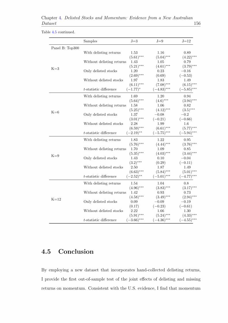
Chapter 4. Delisted Stocks and Momentum: Evidence from a New AustralianDataset 156
Table 4.5 continued.
Samples J=3 J=9 J=12
Panel B: Top300
K=3
With delisting returns 1.53 1.16 0.89(5.61)∗∗∗ (5.04)∗∗∗ (4.22)∗∗∗
Without delisting returns 1.43 1.05 0.79(5.21)∗∗∗ (4.61)∗∗∗ (3.79)∗∗∗
Only delisted stocks 1.20 0.23 −0.16(2.69)∗∗∗ (0.69) (−0.53)
Without delisted stocks 1.97 1.83 1.49(6.11)∗∗∗ (7.08)∗∗∗ (6.15)∗∗∗
t-statistic difference (−1.77)∗ (−4.83)∗∗∗ (−5.85)∗∗∗
K=6
With delisting returns 1.69 1.20 0.94(5.64)∗∗∗ (4.6)∗∗∗ (3.94)∗∗∗
Without delisting returns 1.58 1.06 0.82(5.25)∗∗∗ (4.12)∗∗∗ (3.5)∗∗∗
Only delisted stocks 1.37 −0.08 −0.2(3.01)∗∗∗ (−0.21) (−0.66)
Without delisted stocks 2.28 1.99 1.6(6.59)∗∗∗ (6.61)∗∗∗ (5.77)∗∗∗
t-statistic difference (−2.19)∗∗ (−5.75)∗∗∗ (−5.94)∗∗∗
K=9
With delisting returns 1.83 1.22 0.95(5.76)∗∗∗ (4.44)∗∗∗ (3.76)∗∗∗
Without delisting returns 1.70 1.09 0.85(5.35)∗∗∗ (4.03)∗∗∗ (3.44)∗∗∗
Only delisted stocks 1.43 0.10 −0.04(3.2)∗∗∗ (0.29) (−0.11)
Without delisted stocks 2.50 1.87 1.49(6.63)∗∗∗ (5.84)∗∗∗ (5.01)∗∗∗
t-statistic difference (−2.52)∗∗ (−5.01)∗∗∗ (−4.77)∗∗∗
K=12
With delisting returns 1.54 1.04 0.8(4.96)∗∗∗ (3.83)∗∗∗ (3.17)∗∗∗
Without delisting returns 1.42 0.93 0.73(4.58)∗∗∗ (3.49)∗∗∗ (2.94)∗∗∗
Only delisted stocks 0.09 −0.09 −0.19(0.17) (−0.23) (−0.61)
Without delisted stocks 2.22 1.66 1.30(5.91)∗∗∗ (5.24)∗∗∗ (4.33)∗∗∗
t-statistic difference (−3.66)∗∗∗ (−4.36)∗∗∗ (−4.55)∗∗∗
4.5 Conclusion
By employing a new dataset that incorporates hand-collected delisting returns,
I provide the first out-of-sample test of the joint effects of delisting and missing
returns on momentum. Consistent with the U.S. evidence, I find that momentum

Chapter 4. Delisted Stocks and Momentum: Evidence from a New AustralianDataset 157
profits rely heavily on delisted stocks and their subsequent delisting returns. How-
ever, this effect is reversed in the Top300 by market capitalization, in contrast to
the U.S. findings. Since delisted stocks play little role, if not a positive role, in
driving the average momentum return in the Top300, an easy recommendation for
both researchers and practitioners would be to construct momentum portfolios in
the largest stocks. For practitioners, trading momentum in the Top300 gives them
a higher return, which is also less exposed to the risk of holding stocks with high
delisting possibility. For academics who try to explain momentum, I argue that
they have a bigger task in explaining the robustness of momentum in the Top300
in which the average WML return is much higher than in the U.S. markets. Since
the Top300 group contains the largest stocks that are less exposed to liquidity
risks, the momentum effect in Australia is actually more puzzling.
4.A Appendix: Constructing Fama and French’s
(1993) SMB and HML factors
The three factors of Fama and French (1993) consists of market risk factor (Rm−
Rf ), the size factor (SMB) and the book-to-market factor (HML). SMB, Small
Minus Big, captures the premium that small stocks earn over large ones while
HML, High Minus Low, captures the premium that value stocks earn over growth
stocks. Unlike the U.S. market, the Fama-French factors are not readily available
in Australia. I follow the methodology of Fama and French (1993) and construct
the common risk factors. To ensure that the factors are not affected by the methods
used to account for missing returns as outlined in Section 4.3.4, missing returns
are kept as missing.
To construct the size factor, in June of each year t from 1986 to 2008 all listed
stocks covered in Aspect database are ranked by market capitalizations. I then

Chapter 4. Delisted Stocks and Momentum: Evidence from a New AustralianDataset 158
assign all stocks with market capitalization higher than the median of ASX market
capitalization into big portfolio, B, and the rest into small portfolio, S. To con-
struct the book-to-market factor, all stocks are ranked based on BM values at the
fiscal year end (i.e., June). To avoid undoing weight on small stocks, I follow Fama
and French (2012) and compute BM breakpoints in the group of large stocks. I
exclude all stocks with negative book values of equity. The stocks are categorized
such that the first 30% of stocks (growth stocks) has the lowest BM ratios, L; the
next 40% of stocks is assigned to medium portfolio, M ; and the remaining 30% of
stocks (value stocks) comprise the high BM, H, portfolio.
In the next step, I construct six intersection portfolios (S/L, S/M, S/H, B/L, B/M
and B/H). These portfolios are held for twelve months and monthly value-weighted
returns on those six portfolios are computed from July of year t to June of year
t+ 1. The SMB and HML factors are then calculated as follows.
SMB = 1/3(SmallV alue+ SmallNeutral + SmallGrowth)
− 1/3(BigV alue+BigNeutral +BigGrowth)
HML = 1/2(SmallV alue+BigV alue)− 1/2(SmallGrowth+BigGrowth)

Chapter 5
Conditional Asset Pricing and
Momentum
I find that winner stocks have higher risk exposure to Fama and French (1993)
three factors (FF3F) than loser stocks during good economic times, and therefore
should earn higher expected returns. Employing the conditional FF3F model to
risk adjust returns on winner and loser stocks, I find that this model can reduce
the average momentum alpha by 50% compared to the conventional portfolio-
level estimate. I point out the ‘sample selection bias’ in the existing methodology
of component-level risk adjustment. After correcting for this bias, asset pricing
models examined in this study still cannot fully explain momentum returns.
159

Chapter 5. Conditional Asset Pricing and Momentum 160
5.1 Introduction
The short-term momentum in stock returns of Jegadeesh and Titman (1993) is
one of the greatest challenges to existing asset pricing models. The literature gen-
erally agrees that the unconditional capital asset pricing model (CAPM) of Sharpe
(1964) and Lintner (1965) cannot explain the momentum effect. Jaganathan and
Wang (1996) argue that the unconditional CAPM is not originally developed to
describe a realistic multi-period economy, and hence does not exhibit meaningful
relationships between market betas and expected returns. They show that the
conditional CAPM is powerful in explaining the cross section of average returns.
Recently, Boguth, Carlson, Fisher, and Simutin (2011) find that when the CAPM
is conditioned on contemporaneous realized betas of individual winner and loser
stocks (components), the average momentum alpha declines by 20% to 40% rel-
ative to the unconditional measure. Moreover, the conditional CAPM performs
better than the conditional Fama and French (1993) three-factor (FF3F) model.
There are several curious results left unexplained in the previous research. Firstly,
the reasons why the information of winner/loser stocks’ lagged betas can enhance
the explanatory power of the conditional CAPM are still unclear in Boguth et al.
(2011). Secondly, why their conditional FF3F model does not perform as well as
the conditional CAPM also remains unanswered. This issue may be related to
the third curious finding about the incorrect prediction of FF3F model. Fama
and French (1996) document that the unconditional loadings on their SMB and
HML factors are higher on loser portfolios than winner counterparts, and hence
falsely “predict” negative momentum returns (the reversal effect). No study has
successfully offered justifications for this special failure of the FF3F model in
explaining momentum profits, although this model can rationalize many other

Chapter 5. Conditional Asset Pricing and Momentum 161
anomalies.1
In this study, I provide simple explanations for those curious results. I argue that
the momentum effect is an artifact of the way stocks are selected in the portfolio
such that their true time-varying dynamics are concealed at the aggregate portfolio
level. This argument is consistent with Lo and MacKinlay (1990a) and Lewellen
et al. (2010) who express skepticism about particular methods of sorting stocks,
which can significantly affect the final results.
I find that winner stocks on average load more on market risks during up markets
whereas loser stocks have higher loadings in down markets. The time-series trends
in market loadings of winner and loser stocks also move in opposite directions to
each other over time. But these contrasting dynamics do not appear on the aggre-
gate portfolio return. Since Cooper et al. (2004) show that momentum returns are
lower following market losses, we should expect to see the market beta of winner-
minus-loser (WML) portfolios to be lower when the economy moves from the peak
to the trough.2 But this is not the case for the contemporaneous beta estimated
using monthly portfolio returns. I find that when the economy heads toward reces-
sions, the WML beta computed using aggregate portfolio returns increases by 0.07,
suggesting a rise, not a fall, in momentum returns. On the other hand, the average
WML beta computed using returns on individual stocks (components) shows the
correct direction with a decrease in beta by 0.30 when the economy enters reces-
sions. These observations indicate that Boguth et al.’s (2011) average component
betas can improve the explanatory power of the conditional CAPM because they
capture the true time variation of winner and loser stocks over time.3
1Fama and French (1996, p. 68) find that loser portfolios have higher loadings on SMB andHML factors than winner portfolios. Consequently, they conclude that “the three-factor modelpredicts reversal for the post-formation returns of short-term losers and winners, and so missesthe observed continuation.”
2Grundy and Martin (2001) and Daniel and Moskowitz (2011) also document the lower mo-mentum profitability in bear markets.
3Because the NBER business cycles are dated ex− post, there is a concern about the “look-ahead” bias if one is to use the dates. It should be noted that this study does not use NBERbusiness cycles dates to form trading portfolios, nor does it rely on those dates in estimating

Chapter 5. Conditional Asset Pricing and Momentum 162
Similar to the time-varying dynamics of the market beta, the SMB and HML
factors of Fama and French (1993) also correctly rationalize returns on individual
winner and loser stocks during good economic times. Winner stocks, which act
more like small and distressed firms, have higher exposure to the SMB and HML
risk factors. Therefore, winners should earn higher future average returns and
losers should earn lower average returns, causing positive expected momentum
profits during bull markets. The converse is true when risk loadings are estimated
using aggregate portfolio returns, consistent with Fama and French (1996).4 These
results show that the puzzle of Fama and French (1996) can be solved by looking at
individual stock components. Consequently, I employ the conditional asset pricing
model to risk adjust returns on individual stocks of the portfolio (this method is
briefly called component-level risk adjustment).
Boguth et al. (2011) argue that using the lagged component beta as a conditioning
variable has the advantage of accounting for changing weights of individual stocks
at the end of the ranking period; betas computed using aggregate portfolio returns,
by contrast, miss out this information. Similarly, I argue that the first advantage
of the component-level risk adjustment is that it explicitly captures the change
in weights of individual stocks. It also accounts for the fact that the portfolio’s
composition changes frequently due to rebalancing and delisted stocks. Grundy
and Martin (2001) document that 39.908% of winners and 36.233% of losers are
dropped out of the portfolio at the end of the investment period. Eisdorfer (2008)
notes that on average 10% of stocks in the winner and loser portfolios are delisted
during the investment period, causing the portfolio’s composition at both end
points of the holding period to be different. Finally, the component-level risk
adjustment has an advantage that tests on portfolio returns do not have (even
if we use the component beta as an instrument): it can “undo” the mechanical
conditional asset pricing models. Rather, the study simply uses the business cycle dates todemonstrate the time variation of momentum stocks’ betas.
4Grundy and Martin (2001) show that the factor exposure of winner and loser stocks duringthe investment period is determined by their exposure during the ranking period.

Chapter 5. Conditional Asset Pricing and Momentum 163
method of stock selections of momentum strategies as argued in Lo and MacKinlay
(1990a) and Lewellen et al. (2010).5
To demonstrate the mechanical way of sorting stocks into momentum portfolios
that biases the unconditional alpha upwards, I conduct a small Monte Carlo sim-
ulation in which returns on 4000 stocks are generated by the CAPM (i.e., their
returns are completely explained by the CAPM.) I follow the usual approach to
form momentum portfolios whose average returns are risk-adjusted using the time-
series market model regression. As expected, I find that the alpha is higher than
the average raw momentum return and the null hypothesis of zero (portfolio) al-
pha is rejected 88% of the time at the five percent level. These results are striking
because the CAPM holds exactly for every single stock, but the mechanical way
of sorting stocks causes momentum alphas to be non-zero.6
Applying to CRSP monthly data, I find that when the conditional FF3F model
is used to risk adjust returns on individual winner and loser stocks, the reduction
in average momentum alphas ranges from 14% (for the CAPM) to 50% (for the
FF3F model) compared to the respective portfolio-level estimate. For the typi-
cal 6/1/6 momentum portfolio in which stocks are ranked by their continuously
compounded returns over the past 6 months and then winner-loser portfolios are
held over the next 6 months with one-month skipping period in between, the
conditional FF3F model performs better than the conditional CAPM by reduc-
ing the average alpha by 30bps per month – in contrast to the portfolio-level
evidence. The average component-level alpha from the conditional FF3F model
is reduced to 0.61% per month (t-statistic = 2.13), representing a 50% decrease
5Chordia et al. (2011) and Ang et al. (2010) also argue that applying asset pricing models onindividual constituents of the portfolio can mitigate the critique of Lo and MacKinlay (1990a)about the arbitrary method of sorting stocks. In a study outside the momentum literature,Griffin et al. (2010) (page 3243), who test the efficiency of international exchanges, argue that“an advantage of using individual stocks is that one can allow correlations [between stocks] toswitch sign”.
6I repeat my simulations in which stocks’ returns are now generated by the three risk factorsof Fama and French (1993) downloaded from Ken French’s website. My conclusions do notchange.

Chapter 5. Conditional Asset Pricing and Momentum 164
from the portfolio-level estimate. These findings confirm my conjecture that the
component-level risk adjustment is able to account for the change in weights and
composition of momentum portfolios. As I show in Section 5.4, it also allows for
the fact that the time variation in components’ betas is much bigger than that of
their portfolio counterparts. Consequently, the existing asset pricing models have
higher explanatory power when these facts are accounted for.7
My study is related to Chordia and Shivakumar (2002) who employ a macroe-
conomic model to adjust returns on individual stock components of momentum
portfolios. A more recently related paper is of Wang and Wu (2011) who use the
unconditional FF3F model to risk adjust individual stock returns. In this study, I
point out the ‘sample selection bias’8 in the existing methodology of component-
level risk adjustment, which typically uses 60 months of returns on individual
stocks including the entire ranking period to run regressions.
I argue that using ranking period returns will bias the estimated beta because,
by construction, the momentum strategy selects stocks with the most positive
past returns for winner portfolios and those with the most negative past returns
for loser portfolios. When the ranking period was a bull market, the WML beta
would be positive, while the beta would be negative when the ranking period
7Employing individual stocks as test assets is often believed to incur more estimation errorsthan portfolios. However, relying on this argument to reject the use of individual stocks is notalways right, as argued by Ang et al. (2010) who show that standard errors from firm-level cross-sectional regressions are not higher, and in some cases are even lower, than those from portfolios.Recently, Chordia et al. (2011) also endorse the use of cross-sectional regressions on individualstocks. Both studies focus on the econometrics sides of tests rather than the explanatory power(on momentum anomaly) of asset pricing models. It should also be noted that I do not employcross-sectional but simple time-series regressions. As noted in the discussion of Chordia et al.(2011), since estimated betas do not serve as explanatory variables in my tests there are noerrors-in-variables in the coefficients.
8This bias is not the survivorship or look-ahead bias. I acknowledge that the phrase “sampleselection bias” is loose and subject to debate, but I use it as a convenient way to indicate thebias that is incurred by using ranking period returns, which are determined by the constructionof momentum strategies, as the left-hand side of the regression. I explain this bias in detail inSection 5.4.

Chapter 5. Conditional Asset Pricing and Momentum 165
was a bear market.9 Consequently, if betas are estimated using ranking period
returns, the bias will be positive during bull markets while during bear markets,
the bias will be negative. This bias serves to artificially amplify the dynamics of
estimated betas relative to the true beta, thereby causing all asset pricing models
that account for time-varying risk to completely explain momentum returns.
I correct for this bias by simply excluding ranking period returns from the esti-
mation and find that the magnitude of the bias is much bigger in down markets.
For example, using CRSP data, I find that the bias causes the market beta of
momentum portfolios to be 22% higher during economic expansions (as dated
by the NBER), but 37% lower during contractions. By correcting for the bias,
I find that the results of Chordia and Shivakumar (2002) are reversed.10 With
the bias in place, I confirm their original results that their macroeconomic model
yields the average adjusted momentum return of -2.97% per month. After the bias
correction, this average adjusted return reverses to positive 5.03% per month.
The paper proceeds as follows. The next section reviews related studies in more
details. Section 5.3 describes the data and how I form momentum portfolios.
Section 5.4 presents my main results and motivate the sample selection bias. I
also provide a theoretical perspective on why the component-level risk adjustment
can help improve the explanatory power of asset pricing models. I conclude in
Section 5.5.
9The positive covariance between momentum returns and the market is also documented inGrundy and Martin (2001), Chordia and Shivakumar (2002), Daniel and Moskowitz (2011), andBoguth et al. (2011).
10Chordia and Shivakumar (2002) essentially employ two methods; the first is similar to mineand the second is a two-way dependent portfolio sort between raw and predicted returns. Usingthe second method, Griffin et al. (2003) show that the findings of Chordia and Shivakumar(2002) do not hold in 16 international markets. Similarly, Cooper et al. (2004) find that Chordiaand Shivakumar’s (2002) results from the two-way portfolio sorts are driven by the marketmicrostructure bias of penny stocks. In this study, after excluding penny stocks, I point out thatthe first method of Chordia and Shivakumar (2002) also suffers from sample selection bias.

Chapter 5. Conditional Asset Pricing and Momentum 166
5.2 Related literature
Although the literature on time-varying risk premium has been well developed,
applying the conditional models at individual stock levels is not frequently em-
ployed. In the momentum literature, Chordia and Shivakumar (2002) were among
the first to use a set of macroeconomic variables to adjust returns on individual
winner and loser stocks. In other words, their method is similar to mine, ex-
cept that they do not have risk factors in the model. Chordia and Shivakumar
(2002) find that momentum is strongly related to business cycles as dated by the
NBER and consequently suggest that momentum can potentially be explained by
time-varying expected returns. However, to be explained by rational theories, mo-
mentum payoffs must covary with risk factors. As acknowledged by Chordia and
Shivakumar (2002), the lack of common risk factors in their model constrains their
claims to only the correlation between the predictive power of those variables and
momentum payoffs.
My study builds on their method to incorporate the common risk factors that
have been empirically proved to explain the cross section of returns. I also use
a set of conditional asset pricing models that allow us to tackle the time-varying
betas of individual stocks. My conclusions are therefore more general and the final
momentum payoff can be interpreted as time-varying risk adjusted returns. More
importantly, I find the problem of sample selection bias in the current component-
level adjustment, which occurs because of the time-varying dynamics of winner
and loser stocks over the ranking period. This run-up makes component-level
regressions spurious when the estimation window contains ranking period returns.
After I correct for this problem, the average adjusted return from Chordia and
Shivakumar’s (2002) model reverses from -2.97% per month (t-statistic=-1.52) to
5.03% per month (t-statistic=2.34).

Chapter 5. Conditional Asset Pricing and Momentum 167
Boguth et al. (2011) compute a series of average lagged betas of individual stocks
in the momentum portfolios and use them as another set of conditioning infor-
mation to estimate conditional models at portfolio levels. They show that their
conditional models help reduce momentum alphas by 20% to 40% compared to
the unconditional versions. However, they do not investigate why the average
betas of winner and loser stocks can be good conditioning variables. I provide
explanations for those curious results. In addition, Boguth et al. (2011) estimate
the conditional CAPM and FF3F models at the portfolio levels, which is different
from my method. There are several advantages in my simple risk adjustment at
stock levels. Firstly, as I discuss in later sections, running conditional models at
the individual stock level exploits (1) time-varying betas and the contrasting be-
havior of winner and loser stocks, and (2) the changing composition of, and the
weights on, the sets of stocks that make up the winner and loser portfolios. These
characteristics are not seen by looking at the aggregate portfolio return because
the portfolio is rebalanced frequently. Secondly, since I apply the conditional mod-
els on the return of individual winner and loser stocks, I do not need to include
monthly contemporaneous beta series as another set of conditioning information,
leading to the benefit of parsimony. The final difference is in terms of results.
Boguth et al. (2011)’s conditional CAPM performs better than the conditional
FF3F model in reducing momentum alphas. This can be due to the Fama and
French (1996)’s puzzle of incorrect loadings on SMB and HML factors, which ex-
ist at portfolio levels. As I will show shortly, my component-level risk adjustment
produces lower conditional FF3F alphas due to the correct loadings of FF3F at
individual stock levels.
My study can also be seen as a robust extension of Wang and Wu (2011) who em-
ploy the unconditional FF3F to adjust for the risk of individual winner and loser
stocks. They find that average momentum alphas are reduced by approximately
40%. Although they run rolling regressions at individual stock levels, Wang and

Chapter 5. Conditional Asset Pricing and Momentum 168
Wu (2011) do not estimate the FF3F model under conditioning information and
hence do not account for the time variation in the parameters. Ignoring condition-
ing information may also lead to problematic inferences as pointed out by Boguth
et al. (2011). Boguth et al. (2011) show that running rolling regressions without
conditioning variables will incur “overconditioning” bias to the average momen-
tum alpha. This overconditioning bias incurs because the nonlinearity in payoffs
of winners and losers. In fact, I show that even at the firm level, individual winner
and loser stocks are exposed to the market risk differently in different economic
states, causing the payoffs to be nonlinear. Consistent with Boguth et al. (2011),
I find that conditioning betas on a set of state variables can significantly improve
the explanatory power of asset pricing models. Wang and Wu (2011) also do not
discuss how errors in variables may affect their results. Similar to the problem of
Chordia and Shivakumar (2002), accounting for the sample selection bias increases
the risk-adjusted return in Wang and Wu (2011) by approximately 20%.
5.3 Data and methodology
This study employs monthly returns from every stock in the Center for Research
in Security Prices (CRSP) database from January 1963 to December 2009. Con-
sistent with the literature, I examine stocks with share codes of 10 or 11 and thus
exclude closed-end funds, Real Estate Investment Trusts (REITs), trusts, Ameri-
can Depository Receipts (ADRs), and foreign stocks from the sample. Computed
returns also take into account distribution events such as stock splits or right is-
sues. To ensure that I do not incur any look-ahead bias, I do not apply any filters
to this raw dataset until the construction of momentum portfolios.
As I am interested in testing conditional asset pricing models, I employ instrumen-
tal variables that are common in the literature (Fama and French, 1989). I include
a constant; the dividend yield ratio (DY) computed as the cumulative 12-month

Chapter 5. Conditional Asset Pricing and Momentum 169
dividends divided by the current price index level; the term spread (TERM) cal-
culated as the difference in yields between ten-year and three-month yield spread
in the Treasury market; and the default spread (DEF) which is the difference in
yields between Baa- and Aaa-rated bonds. Data on these state variables, which
are obtained from Amit Goyal’s website11, are also comprehensively examined in
Goyal and Welch (2008). Finally, I obtain the Fama and French (1993) three
factors, namely excess market returns (RM), SMB and HML, from Ken French’s
website.12
Table 5.1 reports summary statistics for three instrumental variables. The mean
value of DEF is the lowest and it also has the lowest standard deviation. The three
variables are also not highly correlated, with the highest correlation of 0.46 between
DY and DEF. These low correlations mean that I do not employ duplicating
state variables and they may provide independent information, if they provide
any information at all.
5.3.1 Constructing momentum portfolios
I follow Jegadeesh and Titman (1993) and construct momentum portfolios. In or-
der to aid comparisons with other conditional models in the momentum literature
(for example, Lewellen and Nagel (2006) and Boguth et al. (2011)), I consider
6/1/6 strategies where stocks are ranked over the past 6 months. Specifically,
at the end of each month, continuously compounded returns on each stock are
computed as a criterion to rank stocks over the past 6 months (formation period).
To be eligible for ranking, stocks must have a return history of 6 months and
be actively traded from the beginning to the end of the formation period. This
restriction is necessary because stocks with invalid returns at both endpoints of
11Amit Goyal’s research data, http://www.hec.unil.ch/agoyal/, accessed 08/06/2011. Ithank Amit Goyal for publicizing the data.
12I also thank Kenneth French for making the data available onhttp://mba.tuck.dartmouth.edu/pages/faculty/ken.french/data library.html.

Chapter 5. Conditional Asset Pricing and Momentum 170
Table 5.1: Descriptive statistics, January 1963 to December 2009
Panel A reports the summary statistics of the three instrumental variables, the dividend yield(DY), the default spread (DEF) and the term spread (TERM). The sample period is fromJanuary 1963 to December 2009. SD is the standard deviation. AC(1) and AC(12) are theautocorrelation with lag 1 and lag 12, respectively. The two right-most columns present thecorrelation between the variables. Panel B shows the statistics of the same variables as wellas the cross-sectional average of winner and loser betas during expansions and contractions, asdated by the NBER business cycles. The last two columns of panel B reports the average changein beta loadings from peak to trough and trough to peak, respectively. The sample period inpanel B is intentionally lengthened from January 1936 to December 2009 since I want to capturemore expansions and contractions of the economy. The firm-level average loading on the marketrisk are constructed as follows. At the end of each ranking period t − 1, the CAPM is run oneach winner and loser stock using returns from t−120 to t−1 (as I will show in later section, thiswindow includes ranking period returns and hence biases the estimated beta. For the purpose ofcomparing between biased beta and non-biased beta (reported in Table 5.7), I present the biasedbeta in this Table). Betas are preserved each month and the value-weighted average across winnerand loser stocks is computed to get the monthly time-series of average betas whose descriptivestatistics are reported in the first three rows of Panel B. I also compute contemporaneous betas onthe momentum portfolios by running 120-month rolling window regressions of portfolio returnson the market risk (Lewellen and Nagel, 2006). I report these portfolio-level betas in rows fourto six of Panel B.
Panel A: Descriptive Statistics (January 1963 to December 2009)
CorrelationMean (%) SD (%) AC(1) AC(12) DEF TERM
DY 3.12 1.18 0.99 0.89 0.46 −0.16DEF 1.04 0.48 0.97 0.56 0.25TERM 1.69 1.52 0.95 0.51
Panel B: Business Cycle Dependence (January 1936 to December 2009)
Expansion Contraction Average ChangeMean SD (%) Mean SD (%) Peak-Trough Trough-Peak
Component-level Winner Betas 1.23 0.26 0.96 0.28 −0.26 0.13Component-level Loser Betas 1.12 0.25 1.26 0.23 0.05 −0.13Component-level WML Betas 0.11 0.43 −0.30 0.45 −0.30 0.26Portfolio-level Winner Betas 1.30 0.11 1.34 0.11 −0.06 −0.05Portfolio-level Loser Betas 1.38 0.20 1.41 0.21 −0.13 −0.01Portfolio-level WML Betas −0.08 0.22 −0.07 0.17 0.07 −0.04DY 3.71% 1.54 4.38% 1.57 0.70% −0.87%DEF 0.97% 0.45 1.29% 0.72 0.52% −0.48%TERM 1.71% 1.25 1.30% 1.31 1.85% −1.85%
ranking period cannot be computed. Moreover, if the stocks are not traded at the
end of the formation period, they cannot be purchased or sold, and thus cannot
be included in the relative-strength portfolio.
Following Jegadeesh and Titman (2002), stocks must also be priced above $5 at
the end of each ranking period t − 1 in order to be included in either winner or
loser portfolios.13 Stocks with market capitalizations in the bottom decile (using
NYSE breakpoints) at time t−1 are also excluded from the examination. Because
13In order to unify the time reference, I denote t as the skipping month (the month before theholding period). Thus, the formation period is from t− 6 to t− 1 and the holding period is fromt+ 1 to t+ 6.

Chapter 5. Conditional Asset Pricing and Momentum 171
I am interested in testing asset pricing models on individual stock returns, I en-
sure meaningful regression estimates by requiring that stocks must also have 24
valid returns over the past 60 months to be ranked at time t − 1. These require-
ments do not induce look-ahead bias as all historical information is known prior
to the holding period. If a stock is delisted from the exchange, I will use CRSP’s
corresponding delisting return in the last month of returns in the holding period.14
Stocks are then grouped into deciles where the top decile consists of the best
performing stocks (winners) and the bottom decile contains the worst performing
stocks during the ranking period (losers). In the next 6 months (referred to as
holding or investment period), the momentum strategy enters a long position in an
equally-weighted portfolio of winners and a short position in an equally-weighted
loser portfolio.
In order to avoid bid-ask bounce and price pressure, I follow the literature to
introduce one-month skipping period between formation and holding periods (Je-
gadeesh (1990), Lo and MacKinlay (1990b), Boudoukh et al. (1994) and Grinblatt
and Moskowitz (2004)).15 Following Jegadeesh and Titman (1993), the strategies
are followed each month, and thus overlapping portfolios are constructed.
5.4 Portfolio- versus component-level risk adjust-
ment
In this section, I first compliment the literature that performing risk adjustments
using the conditional CAPM and FF3F models on aggregate portfolio returns
14This practice follows the existing literature (e.g. Eisdorfer (2008)). Beaver et al. (2007)document that the majority of delisting distribution payments are made in the month of thedelisting. Therefore, they suggest that assuming delisting returns are realized immediately afterthe delisting month is usually reasonable.
15Lo and MacKinlay (1990b) show that bid-ask bounces may cause short-term reversals inwhich losers may become winners and vice versa.

Chapter 5. Conditional Asset Pricing and Momentum 172
cannot explain the momentum effect. I then proceed to applying those models on
returns of individual winner and loser stocks (components) that comprise momen-
tum portfolios.
5.4.1 Portfolio-level risk adjustment
Panel A of Table 5.2 reports raw average returns on the 6/1/6 momentum strategy.
The strategy yields the average return of 1.01% per month with an associated t-
statistic of 4.87, which is statisticaly significant at the 1% level. This magnitude
of return is comparable to that of the existing studies (e.g. Jegadeesh and Titman
(2001)). Panel B shows the alpha from the following unconditional time-series
regression:
rWML,t = αWML + β>WMLf j,t + ε (5.1)
where rWML,t is the return on winner-minus-loser portfolio, f jt represents common
risk factors, namely the excess market return (rm) or the Fama and French (1993)
three factors (FF3F). αWML is reported as the unconditional risk-adjusted return
at portfolio levels.
Panel B of Table 5.2 confirms previous research that unconditional asset pricing
models cannot explain the momentum effect. The unconditional CAPM alpha is
1.04% per month, which is slightly higher than the average raw return in panel
A. Of note is the failure of the FF3F model, whose WML alpha is much higher
than that of the CAPM. Consistent with Fama and French (1996), the intercept
on the loser portfolio is strongly negative (-0.74%), thereby inflating the average
winner-minus-loser alpha to 1.23% per month (t-statistic = 5.90), which is higher
than both the CAPM alpha and the average raw momentum return of 1.01% per
month.

Chapter 5. Conditional Asset Pricing and Momentum 173
Panel C reports the alpha from conditional multi-factor models:
rWML,t = αWML +K∑j=1
(β>WML,jZt−1)f jt + εt (5.2)
where rWML,t is the return on the winner-minus-loser portfolio and f jt represents
common risk factors. Zt−1 is the row vector of lagged instrumental variables
including a constant. αWML and βWML are the constant loadings to be estimated
while Zt−1βWML,t−1 are the conditional risk loadings on the factor. The main
advantage of this econometric specification, which is also used in Ferson and Schadt
(1996) and Boguth et al. (2011), is the ease of interpretation.16 Specification (5.2)
says that the conditional model is expressed as an unconditional multi-factor model
consisting of common risk factors and their corresponding interactions with state
variables. If the model is correctly specified, αWML is expected to be equal to zero.
Panel C shows that conditional models offer no improvements in pricing errors.
The conditional CAPM alpha is 1.04% per month with an associated t-statistic of
4.67, which is equal to that of the unconditional model. Similarly, the conditional
FF3F alpha is 1.19% per month (t-statistic = 5.55), which is only 4 bps lower than
the unconditional estimate.
In unreported tables, I compute Gibbons-Ross-Shanken (GRS) F -tests of inter-
cepts on 10 momentum portfolios, which show that conditional models perform
slightly better in explaining momentum profits than their unconditional counter-
parts. The GRS test shows that the conditional FF3F model produces the lowest
F -statistic of 5.23, compared with 5.81 for the conditional CAPM. Nevertheless,
consistent with the literature (Grundy and Martin, 2001), conditional models that
are applied at the portfolio level still do not fully rationalize the momentum effect.
16Shanken (1990) and Ferson and Harvey (1999) also allow the alpha to be time-varying withthe conditioning information.

Chapter 5. Conditional Asset Pricing and Momentum 174
I therefore turn into the component-level risk adjustment of Chordia and Shivaku-
mar (2002) in which the focus is now on the individual constituent of winner and
loser portfolios.
Table 5.2: Portfolio-level risk adjustment
This table reports risk-adjusted returns on momentum portfolios using unconditional models(panel B) and conditional models (panel C) from January 1963 to December 2009. All returns(reported in percentages) are risk-adjusted (i.e. estimated intercepts) by regressing excess rawreturns on the risk factors (Equation 5.1) and their interactions with the state variables (Equation5.2). The factors are excess returns on the market (RM ) or the Fama and French’s (1993) threefactors (FF3F). Three state variables are dividend yield, term spread and the default spread.WML is the return on winner− loser portfolios. Stocks are required to have at least 24 monthsof valid returns over the past 60 months to be ranked. t− statistics calculated using Newey andWest (1987) standard errors with six lags are reported in parentheses. ∗, ∗∗, ∗ ∗ ∗ represent thesignificance levels at 10%, 5% and 1%, respectively.
Models Winners Losers WML
Panel A: Raw returnsRaw Returns 1.57 0.56 1.01
(6.71)∗∗∗ (2.52)∗∗ (4.87)∗∗∗
Panel B: Unconditional risk adjustmentCAPM 0.53 −0.52 1.04
(3.22)∗∗∗ (−3.18)∗∗∗ (5.23)∗∗∗
FF3F 0.49 −0.74 1.23(4.09)∗∗∗ (−5.61)∗∗∗ (5.90)∗∗∗
Panel C: Conditional risk adjustmentCAPM 0.58 −0.46 1.04
(3.30)∗∗∗ (−2.54)∗∗∗ (4.67)∗∗∗
FF3F 0.52 −0.68 1.19(4.55)∗∗∗ (−4.73)∗∗∗ (5.55)∗∗∗
5.4.2 Component-level versus portfolio-level betas
In this subsection, I examine the difference in dynamics of betas between individ-
ual stocks and aggregate portfolio returns. I point out that the time variation of
average betas of individual winner and loser stocks is much higher than that of
aggregate portfolios. These time-varying dynamics cannot be seen at the portfolio
level because momentum portfolios re-balance frequently, causing their composi-
tions and individual stocks’ market capitalizations to change on a monthly basis.
Without loss of generality, the following market model regression is run for each
stock i belonging to winner or loser portfolios using 120 months of its returns prior
to the ranking period.

Chapter 5. Conditional Asset Pricing and Momentum 175
ri,t = α + βirm,t + εi (5.3)
where ri,t is the excess return on stock i; rm,t is the excess returns on the market.
Beta loadings for individual stocks are preserved in each month and the monthly
value-weighted average of betas across the winner and loser stocks are computed,
taking into account the market capitalization of each stock at the end of ranking
periods. For the comparison across betas at different levels, I use value weights
by market capitalization of stocks at the end of ranking period when reporting
average betas and their graphs. In order to avoid losing too much data, I use 60-
month window in the first 120 months of a stock’s life, and then employ the full
120-month window afterward. As argued by Boguth et al. (2011), the advantage
of computing betas in this way is that I do not leave out the information in the
weight (i.e. market capitalization) of the individual components. I plot the time
series of component-level betas in the first graph of Figure 5.1. Since I wish to
capture more economic contractions and expansions, the sample period in this
analysis is extended between January 1936 and December 2009.
I also plot average WML betas on ‘hypothetical’ portfolios, which are equivalent
to the average component beta. At the end of each ranking period t−1, I compute
value-weighted average returns on the WML portfolio over the past 120 months
prior to the six-month ranking period (from t−126 to t−6). I then regress these 120
months of WML portfolio returns on the excess market return and obtain the beta.
I repeat this ‘portfolio-level regression’ as I form a new portfolio in the following
month. Because the portfolio beta should be equal to the value-weighted average of
individual stocks’ betas, the betas of these hypothetical portfolios should be similar
to those computed at the individual component levels in the first graph. In fact,
the correlation coefficient between the average firm-level betas and hypothetical
portfolios’ betas is 0.98 (not tabulated).

Chapter 5. Conditional Asset Pricing and Momentum 176
Hypothetical portfolio betas are plotted in the second graph of Figure 5.1. I call
these portfolio betas hypothetical because they are different from those computed
using returns on actual Jegadeesh and Titman’s (1993) momentum portfolios,
which do not take into account changes in stock compositions and weights at
the end of each ranking period. The purpose of constructing these hypothetical
portfolios is to show that firm-level risk adjustment is similar to portfolio-level risk
adjustment as long as changes in the portfolio composition are properly accounted
for.
In order to compare component-level betas with the contemporaneous portfolio
betas of Lewellen and Nagel (2006), I also plot their portfolio betas of the actual
WML portfolio in the third graph. These market betas are computed by running
120-month rolling regressions of average monthly WML returns on the market risk
(again, I use only 60 months of returns in the first 120 months). Lewellen and
Nagel (2006) argue that this method can capture the effect of time-varying betas
as long as betas are fixed within the window.
The first two graphs of Figure 5.1 show that the average component-level WML
beta varies dramatically over time. They are even more volatile during crisis
periods such as the early 2000s market crash and the recent Global Financial Crisis
between 2007 and early 2009. These time-varying dynamics of WML portfolio beta
computed using returns on individual stocks indicate that if we treat the aggregate
momentum portfolio as a test asset and run model (5.3) as one-shot regression to
obtain a single estimate, we will miss out the important time variation in the beta
of individual momentum stocks at the end of the ranking period. This problem
still exists even when we estimate betas using rolling-window regressions on the
monthly portfolio return (Lewellen and Nagel, 2006).17
17Boguth et al. (2011) show that the methods to estimate conditional models in these studiesgive problematic inferences, as they suffer from “over-conditioning bias” in which the conditioninginformation was not observed by investors at time t− 1.

Chapter 5. Conditional Asset Pricing and Momentum 177
The first three rows of Panel B of Table 5.1 report the average market beta of indi-
vidual winner and loser stocks (components) computed at the end of each ranking
period. Winner stocks load more on the market than losers during economic ex-
pansions (1.23 versus 1.12), suggesting that WML portfolios should earn higher
expected return in the holding period. Loser stocks on the other hand have the
average market loading of 1.26 during contractions, which is higher than 0.96 of
winner stocks, indicating that the WML portfolio should earn lower average return
in the holding period. The last two columns of Table 5.1 show the movements of
betas from the peak to the trough of the economy and vice versa. Consistently,
winner betas on average decrease by 0.26 when the market moves from the peak
to the trough while they increase by 0.13 during recovery periods. The movement
of loser betas is just the opposite. When the economy falls into recessions, the
average beta of loser stocks increases by 0.05. But their betas decrease by 0.13
when the economy heads toward the next peak. These contrasting dynamics of
winners and losers suggest that (1) the betas of winner and loser stocks (compo-
nents) are time-varying with the market states, and (2) a closer examination of
the risk exposure of individual stocks may give us a better understanding of the
underlying risk of momentum portfolios.

Chapter 5. Conditional Asset Pricing and Momentum 178
Figure 5.1: Time-series betas of momentum portfolios
The figure plots the time-series market beta on 6/1/6 winner-minus-loser (WML) portfoliosfrom January 1936 to December 2009 (the sample period is extended to 1936 to capture moreeconomic expansions and contractions). The first graph plots the value-weighted averageloadings of individual stocks (components) in the WML portfolio, corrected for sampleselection bias. At the end of each ranking period, 120 months (from t − 120 − 6 to t − 6)of excess returns on each stock i in the winner and loser portfolios is regressed against theexcess returns on the market. The betas are preserved each month and the value-weightedaverage of betas across winner and loser stocks are computed in that month taking intoaccount the market capitalization of each stock at the end of ranking periods. The secondgraph plots the average betas on the hypothetical portfolios. At the end of each rankingperiod, I compute the weighted average returns on winner and loser stocks over the past120 months (t − 120 − 6 to t − 6). This gives us 120 months of ‘portfolio’ returns, whichare then regressed on the excess market return to obtain portfolio-level beta at the end ofthe ranking period. I repeat this portfolio formation and the regression test as I form anew Jegadeesh and Titman’s (1993) overlapping portfolio in the following month. Since theportfolio beta should be equal to the weighted average of individual stocks’ betas, I expecthypothetical portfolio betas and firm-level betas to be highly correlated. In fact, the correlationbetween these two time-series of betas is 0.98. The third graph plots the contemporaneousbetas as in Lewellen and Nagel (2006), which are computed by running 120-month rollingwindow regressions of monthly WML portfolio returns on the market. In order to use alldata, I employ windows of 60 months in the first 120 months and then the full 120 months af-terward. Vertical lines represent the peaks and troughs of business cycles as dated by the NBER.

Chapter 5. Conditional Asset Pricing and Momentum 179
The third graph of Figure 5.1 shows the contemporaneous market beta on the ag-
gregate value-weighted momentum portfolio. Compared with the first two graphs,
there is much less time variation at the portfolio level, consistent with Lewellen
and Nagel (2006). Moreover, the time-series trend also moves in the opposite
direction to that at component levels, especially during crisis periods. For in-
stance, the contemporaneous portfolio-level beta trended downwards during the
early 2000s market crash whereas the average component-level beta trended up-
ward. In fact, the correlation coefficient (not reported) between component-level
betas and portfolio-level betas is -0.14.
Panel B of Table 5.1 quantifies the trend of portfolio-level betas (three middle
rows). In contrast to average component-level betas, the average portfolio-level
winner beta is lower than that of loser’s during economic expansions (1.30 versus
1.37), suggesting that the momentum portfolio should earn low (or negative) ex-
pected return. I also see similar trends during economic contractions, which cause
the aggregate WML portfolio beta to be similar in both states of the economy
(with -0.08 in expansions and -0.07 in contractions). These results show that the
contemporaneous portfolio-level beta computed using monthly portfolio returns
does not vary over time, and therefore the contrasting dynamics in the betas of
winner and loser stocks (components) do not appear in the portfolio-level beta.
My view is that the movement of market betas computed on aggregate monthly
portfolio returns is counter-intuitive to what we know from the momentum liter-
ature. Given that Cooper et al. (2004) show that momentum returns are lower
following market losses, we should expect to see the beta on WML portfolios to
decrease when the economy moves from the peak to the trough. This is not the
case for portfolio-level betas. The last two columns of Panel B of Table 5.1 shows
that when the economy moves from the peak to the trough, the portfolio-level
WML beta increases by 0.07, indicating a rise, not a fall, in momentum returns.

Chapter 5. Conditional Asset Pricing and Momentum 180
On the other hand, the average component-level WML beta shows the correct di-
rection with a decrease in beta by 0.30 when the market heads toward the trough.
This is another support for the use of component-level risk adjustments.
The variance of component-level betas, hypothetical betas, and portfolio-level be-
tas are 0.159, 0.146, and 0.044, respectively (not tabulated). I test the hypothesis
that the variance of betas is statistically equal to zero using the delta method
corrected for autocorrelations of betas as described in Cochrane (2005). The t-
statistics of the variance in the first, second, and third series of betas are 7.42,
5.85, and 2.88, respectively. The variance of portfolio-level betas has the lowest t-
statistic, indicating that it is not volatile enough to describe the true time-varying
dynamics of momentum stocks’ betas. I also compute average conditional betas
from the Ferson and Schadt’s (1996) conditional market model (in which model
(5.3) has the market return and its interactions with state variables); my conclu-
sions in this section do not change.
The fact that the time variation of components’ betas cannot be seen on the
aggregate portfolio return indicates that applying conditional asset pricing models
on aggregate portfolio returns will miss out the important dynamics of individual
stocks. The contemporaneous portfolio-level beta in the third graph is consistent
with the finding of Lewellen and Nagel (2006, p. 291) that portfolio betas “do vary
considerably over time – just not enough to explain large unconditional pricing
errors”. However, looking at component-level betas we can see a large variation
in the average WML betas, which suggests that a potential source of alpha can
be detected at this level. My findings are consistent with Boguth et al. (2011)
who argue that the component beta uses the important information of the weights
of individual stocks at the end of ranking period whereas portfolio-level betas do
not account for changing portfolio weights (although they do not make the above
points about the dynamics of component-level betas). I provide a more formal
theoretical argument for the component-level risk adjustment in Subsection 5.4.4.

Chapter 5. Conditional Asset Pricing and Momentum 181
5.4.3 Component-level risk adjustment and sample selec-
tion bias
In this subsection, I employ unconditional and conditional asset pricing models
(Models (5.1) and (5.2), respectively) to adjust for the risk of individual stocks
(components) in momentum portfolios. The method is first used by Chordia and
Shivakumar (2002) and later adopted by Wang and Wu (2011). Besides employing
conditional asset pricing models, my methodology also differs from theirs in two
ways. First, for reasons explained below, I use estimation windows prior to the
ranking period. Second, in order to maintain some variations in returns on risk
factors and conditioning variables, I employ 120-month windows instead of 60-
month windows to estimating asset pricing models.18
My component-level risk adjustment proceeds as follows. Momentum portfolios
are formed normally and the constituents (components) of the portfolio are exactly
the same as those in Table 5.2. But during the six-month holding period from t+1
to t+ 6, returns on each individual stock i belonging to winner or loser portfolios
are risk-adjusted using the following general model. The process of computing
portfolio returns then proceeds normally just as we form the raw portfolio.
radji,t = ri,t − rf −K∑j=1
(β>ijZt−1)f jt (5.4)
where β>ij is estimated using the past 120-month returns prior to the ranking
period (i.e., individual stock returns from t− 120− 6 to t− 6. The reason for this
exlusion of six-month ranking period returns will be explained shortly). Stocks
are required to have at least 24 valid observations in the estimation period. (To
ensure results are comparable between tables, this constraint was also in place
18In the earlier version of my paper, I also use fixed 60-month windows of stock returns andmy conclusions do not qualitatively change. Subsection 5.4.7 also employs extending-windowestimations to which my conclusions remain robust.

Chapter 5. Conditional Asset Pricing and Momentum 182
when I formed the raw momentum portfolio.) In order to avoid losing too much
data, I use 60-month windows of returns in the first 120 months and then use
the full 120-month window afterwards. Risk factors, f jt, are excess returns on
the market (rm) or the Fama and French three factors (FF3F). State variables,
Zt−1, are dividend yield, term spread, and the default spread. Before I discuss the
main results of this risk adjustment in Table 5.5, I should first note the differences
between my methodology and that of Chordia and Shivakumar (2002), which is
mainly the exclusion of ranking period returns from the estimation.
Measurement rrrors
The estimation of conditional models at individual stock levels may raise con-
cerns about errors-in-variable (EIV) biases. I note that although the firm-level
risk adjustment has been used in a few momentum studies, EIV is not extensively
discussed. First of all, there is an EIV bias in usual standard errors. Cochrane
(2005) shows that the correct standard error can be calculated in a GMM frame-
work. Assuming that the errors are i.i.d., the variance of estimated alphas can be
computed by the following formula:
var(α) =1
T(1 + µ>f Ω−1
f µf )Σ (5.5)
where µf is K × 1 mean vector of the risk factors; Ωf is the variance-covariance
matrix of the risk factors and Σ is the residual covariance matrix.19 I find that
EIV causes standard errors to be slightly higher, and hence making the t-statistic
slightly smaller. Consistent with the literature (see Chordia et al. (2011) for a
discussion), employing corrected standard errors does not affect any of the conclu-
sions. Nevertheless, all standard errors of risk-adjusted returns in this paper are
calculated using Equation (5.5).
19If the alpha is estimated using conditional models, f will include the risk factors and theirinteractions with the state variables.

Chapter 5. Conditional Asset Pricing and Momentum 183
Using individual stocks as test assets is often thought to incur more estimation
errors than portfolios. However, this argument is not really true as pointed out
by Ang et al. (2010), who show that standard errors from component-level cross-
sectional regressions are not higher, and sometimes are even lower, than those from
portfolios. Recently, Chordia et al. (2011) also endorse the use of cross-sectional
regressions on individual stocks. Both studies focus on the econometrics sides of
tests rather than the explanatory power (on momentum anomaly) of asset pricing
models. It should also be noted that I do not employ cross-sectional but simple
time-series regressions. As noted in the discussion of Chordia et al. (2011), since
estimated betas do not serve as explanatory variables in my tests there is no EIV
in the coefficients.
Readers not familiar with how momentum strategies rebalance may raise concerns
about the difference between component-level betas and portfolio-level betas. The-
oretically, portfolio betas should be equal to value-weighted averages of individual
stocks’ betas. However, due to the fact that individual stocks’ weights and compo-
sition of momentum portfolios change frequently, the beta computed on aggregate
portfolio returns will be different from that computed at the end of each ranking
period. The portfolio’s composition can change not only because the momen-
tum strategy is rebalanced monthly (Grundy and Martin (2001) document that
39.908% of winner portfolio’s composition change each month and this statistic
for loser portfolios is 36.233% due to rebalancing), but also because of stocks be-
ing delisted during the holding period. Eisdorfer (2008) notes that 10% of stocks
in the winner and loser portfolios are delisted between 1975 to 2005, causing the
portfolio’s composition at the end of formation period to be different from that
during the investment period. My hypothetical portfolios (see the second graph
of Figure 5.1) show that if we could compute portfolio-level betas at the end of
each ranking period (before we form the next overlapping portfolio), there would
be virtually no difference between component-level betas and portfolio-level betas.

Chapter 5. Conditional Asset Pricing and Momentum 184
Sample selection bias
In the momentum context, betas from time-series regressions may be biased, not
because of being estimated at component levels, but due to the inclusion of rank-
ing period returns in the regression. The momentum strategy mechanically selects
stocks with the most positive returns over the ranking period into winner port-
folios and those with the most negative returns over the same period into loser
portfolios. Consequently, if we include ranking period returns as the left-hand
side of regressions, the variable is no longer randomly selected, thereby causing
the regression assumptions to be violated. Because winner and loser betas vary
through time as shown in Figure 5.1 and the Panel B of Table 5.1, the magnitude
of this bias is dependent on the market states. In order to see this, without loss of
generality, we can resort to the fundamental representation of measurement error
in the estimated CAPM βit for each component of the WML portfolio as follows:
βit|t−1 − βit =
∑t−S−1s=t−S−T0(rm,s − rmt) · εit∑t−S−1s=t−S−T0(rm,s − rmt)2
(5.6)
where T0 is the estimation window (e.g., 120 months); S is the finishing month of
the estimation window (e.g., if S = 0, I include ranking period returns in the esti-
mation whereas if S = 6, I exclude ranking period returns); rmt = T−10
∑t−S−1s=t−S−T0 rm,s
is the mean of the market return over the estimation period; βit is the true beta;
and εit is the idiosyncratic component of the market model regression. Grundy
and Martin (2001) show that the idiosyncratic return of a stock is the driving force
for it to be a winner or loser stock. Because we are classifying stocks as either
“winners” or “losers” on the basis of their returns over the ranking period, we can

Chapter 5. Conditional Asset Pricing and Momentum 185
appeal to the theory of order statistics20 to assert that for winner stocks, εW will
be positive while for loser stocks, εL will be negative.
As is usual for showing the unbiased estimator of OLS, if we assume that εi,t is
independent of the regressor rm,t, which is a common assumption when dealing
with stochastic regressors (see Section 8.2, p. 207-208 of Hamilton (1994)), we
establish the typical result that the OLS beta is unbiassed (in Equation (5.6),
E(βit|t−1) = βit).
However, in the momentum context, the assumption that rm,t is independent of εit
is clearly indefensible when ranking period returns are included in the estimation.
To see this note that because we are selecting extreme winners and losers, εW,t and
εL,t will be positive and negative, respectively. If the ranking period was a bull
market (formally, let the discrete state indicator Ss = 0 correspond to a month that
is a bull market) then E((rm.s − rmt)εW,s|Ss = 0) > 0 and E((rm.s − rmt)εL,s|Ss =
0) < 0 (for s = t − S + 1, . . . , t − 1), while for bear markets (i.e., Ss = 1)
E((rm.s − rmt)εW,s|Ss = 1) < 0 and E((rm.s − rms)εL,s|St = 0) > 0. This will bias
the results, and I summarize the direction of bias in the table below.21
20When we have a sample of N observations from some distribution fX(x) and we or-der the observations from smallest to largest, X1 = minX1, X2, . . . , XN and XN =maxX1, X2, . . . , XN then the density of the k-th order statistic is given by:
fX(k)(x) = i
(n
k
)[FX(x)]k−1[1− FX(x)]N−kfX(x)
where, for example, the density of the minimum return X(1) equals
fX(1)= fX(x) · [1− FX(x)]N−1 · n!
1!(n− 1)!
which is the unconditional density evaluated at x multiplied by the probability that all of theother N − 1 outcomes are greater than that x, and the number of ways this can be achieved,and where FX(x) denotes the cumulative distribution function of X. As the number of drawsincreases the density of the first order statistic shifts to the left, while the density of the highestorder statistic shifts to the right. If the mean of X is zero, as in the case of the regression residual,this means that the lower order statistics (corresponding to loser stocks) have a negative mean,while the higher order stocks (corresponding to winner stocks) have positive means.
21The positive covariance between εi,t for momentum portfolios and the market is also doc-umented in Grundy and Martin (2001), Chordia and Shivakumar (2002), Cooper et al. (2004),Boguth et al. (2011), and Daniel and Moskowitz (2011).

Chapter 5. Conditional Asset Pricing and Momentum 186
Direction of sample selction bias
Market Portfolios β Bias
BullWinner +Loser −WML +
BearWinner −Loser +WML −
Note: this table summarizes the direction of bias on component betas when they are estimated
using ranking period returns. “+” denotes upward trends while “−” denotes downward trends.
The bias will cause winner betas to be biased upwards while loser betas are biased
downwards during economic expansions, and vice versa for contracting periods
in which winner betas are biased downwards and loser betas are biased upwards.
Because the direction of bias in WML betas is positively related to the market
states, any asset pricing model that accounts for time-varying risks can completely
explain momentum returns (if ranking period returns are included in the estima-
tion). In order to avoid this problem, I estimate betas in Equation (5.4) using
120 months of returns on individual stocks prior to the ranking period (S = 6).
Holding period returns from t+ 1 to t+ 6 will then be risk-adjusted using Equa-
tion (5.4) (i.e., I skip the six-month ranking period before predicting returns in
the holding period).22
To study the size of the bias and how it can be corrected by excluding ranking
period returns from the estimation, I undertake a small Monte Carlo experiment.
I fit a regime switching model to the market returns in which the conditional
distribution of the market depends on the state variable St, which varies between
periods of bull markets when returns have high mean and low variance, and bear
markets when returns have high variance and a slightly negative mean.23 In this
22I thank Jeffrey Wooldridge for a discussion on this issue. In the early version of this paper,I also employed the beta adjustment of Vasicek (1973) to which my results again remain robust.All unreported results are available upon request.
23In particular I use the model of Hamilton (1989), which has been applied in a number ofstudies to stock returns, including Turner et al. (1989). This model has also been applied tostudying long-run mean reversion by Kim et al. (2001) and portfolio selection by Ang and Bekaert(2002).
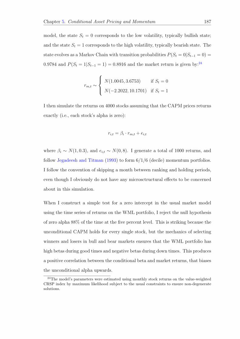
Chapter 5. Conditional Asset Pricing and Momentum 187
model, the state St = 0 corresponds to the low volatility, typically bullish state;
and the state St = 1 corresponds to the high volatility, typically bearish state. The
state evolves as a Markov Chain with transition probabilities P (St = 0|St−1 = 0) =
0.9784 and P (St = 1|St−1 = 1) = 0.8916 and the market return is given by:24
rm,t ∼
N(1.0045, 3.6753) if St = 0
N(−2.2022, 10.1701) if St = 1
I then simulate the returns on 4000 stocks assuming that the CAPM prices returns
exactly (i.e., each stock’s alpha is zero):
ri,t = βi · rm,t + ei,t
where βi ∼ N(1, 0.3), and ei,t ∼ N(0, 8). I generate a total of 1000 returns, and
follow Jegadeesh and Titman (1993) to form 6/1/6 (decile) momentum portfolios.
I follow the convention of skipping a month between ranking and holding periods,
even though I obviously do not have any microsctructural effects to be concerned
about in this simulation.
When I construct a simple test for a zero intercept in the usual market model
using the time series of returns on the WML portfolio, I reject the null hypothesis
of zero alpha 88% of the time at the five percent level. This is striking because the
unconditional CAPM holds for every single stock, but the mechanics of selecting
winners and losers in bull and bear markets ensures that the WML portfolio has
high betas during good times and negative betas during down times. This produces
a positive correlation between the conditional beta and market returns, that biases
the unconditional alpha upwards.
24The model’s parameters were estimated using monthly stock returns on the value-weightedCRSP index by maximum likelihood subject to the usual constraints to ensure non-degeneratesolutions.

Chapter 5. Conditional Asset Pricing and Momentum 188
When I estimate betas using either the component-level beta or the hypothetical
portfolio return that include the ranking period return (with the sample selection
bias), I find a statistically significant but negative momentum effect. In fact, I
reject the null hypothesis in 83% of the samples at the five percent level, but
of course with the negative average momentum return. The negative return is
consistent with the findings of Chordia and Shivakumar (2002).
However, when I construct the test using component-level betas (or equivalently
based on hypothetical portfolio returns) but I only use pre-ranking period returns,
I only reject the null hypothesis 5.36% of the samples at the five percent level.
These findings provide strong support to my recommendation to estimate beta
using component-level returns, but to include only pre-ranking period returns –
anything else would lead to substantial bias in the test statistic.
To further investigate how excluding ranking period returns helps avoid the bias,
Table 5.3 reports the summary statistics, based on the Monte Carlo simulation,
for betas estimated using 120 months of pre-ranking period returns (correcting for
the sample selection bias) and betas estimated using 120 months of pre-holding
period returns (including ranking period returns, and hence incurring the sample
selection bias), and then see how these betas are close to the true beta.
Table 5.3: Bias in estimated betas: Monte Carlo simulation
This table reports summary statistics for CAPM betas estimated from Monte Carlo simula-tions, which are described in the text. True-β denotes the beta used to simulate stock returns.Pre-Holding-β denotes the average beta estimated using 120 months of returns on individualstocks (components) that include the ranking period. Pre-Ranking-β denotes the average betaestimated using 120 months of returns on individual stocks, but the estimation window does notinclude the ranking period.
Winner Loser
True-β Pre-Holding-β Pre-Ranking-β True-β Pre-Holding-β Pre-Ranking-β
Bull Market 1.0370 1.0539 1.0370 0.9636 0.9470 0.9634Bear Market 0.9427 0.8166 0.9425 1.0584 1.1860 1.0583Unconditional 1.0211 1.0143 1.0210 0.9796 0.9869 0.9794
Table 5.3 shows that betas estimated using pre-ranking period returns (the third
column) are almost equal to the true beta (that I use to simulate stock returns
from the CAPM) whereas betas estimated with ranking period returns (the second

Chapter 5. Conditional Asset Pricing and Momentum 189
column) are biased. Table 5.3 also reaffirms my analysis of the direction of bias
in betas. During a bull (bear) market, the average return over the ranking period
will generally be higher (lower) than in the distant past (and recall that I use
estimation windows between 5 and 10 years of monthly returns), and for winner
(loser) stocks I will have positive (negative) residuals. This means that the bias
in estimated pre-holding betas will be positive for winner stocks and negative for
loser stocks during up markets, while it will be negative for winner stocks and
positive for loser stocks during down markets. This bias will serve to artificially
amplify the dynamics of estimated betas relative to the true beta dynamics.
Note that the positive unconditional alpha is driven by the positive covariance
between subsequent betas and the market returns (as shown in Subsection 5.4.4):
during bull markets the WML portfolio will have high betas, while during bear
markets the WML portfolio will typically have negative betas. Because of the (de-
liberate) stock selection of momentum strategies over the ranking period, during
bull markets the estimated WML portfolio beta will be even higher than the true
WML beta on average, and during bear markets the estimated WML beta will
be more negative than the true WML beta. Consequently, the estimated alpha
adjusting for time-varying risks will be too low or even negative, suggesting that
the dynamics of beta artificially account for more of the estimated unconditional
alpha than the conditional CAPM can actually explain.
Empirically, Table 5.4 uses CRSP data and shows the magnitude of sample selec-
tion bias in different NBER business cycles by comparing the difference between
pre-holding period betas (with the bias) and pre-ranking period betas (without
the bias). Consistent with my conjecture, the pre-holding period betas are on
average higher than their pre-ranking counterparts during expansions. During
contractions, pre-holding betas are biased downwards and much lower than the
pre-ranking-period estimates. For example, the difference in market beta of mo-
mentum portfolios between the pre-holding period and pre-ranking period is 0.02
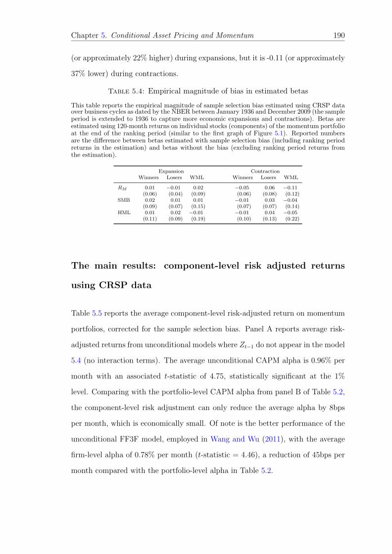
Chapter 5. Conditional Asset Pricing and Momentum 190
(or approximately 22% higher) during expansions, but it is -0.11 (or approximately
37% lower) during contractions.
Table 5.4: Empirical magnitude of bias in estimated betas
This table reports the empirical magnitude of sample selection bias estimated using CRSP dataover business cycles as dated by the NBER between January 1936 and December 2009 (the sampleperiod is extended to 1936 to capture more economic expansions and contractions). Betas areestimated using 120-month returns on individual stocks (components) of the momentum portfolioat the end of the ranking period (similar to the first graph of Figure 5.1). Reported numbersare the difference between betas estimated with sample selection bias (including ranking periodreturns in the estimation) and betas without the bias (excluding ranking period returns fromthe estimation).
Expansion ContractionWinners Losers WML Winners Losers WML
RM 0.01 −0.01 0.02 −0.05 0.06 −0.11(0.06) (0.04) (0.09) (0.06) (0.08) (0.12)
SMB 0.02 0.01 0.01 −0.01 0.03 −0.04(0.09) (0.07) (0.15) (0.07) (0.07) (0.14)
HML 0.01 0.02 −0.01 −0.01 0.04 −0.05(0.11) (0.09) (0.19) (0.10) (0.13) (0.22)
The main results: component-level risk adjusted returns
using CRSP data
Table 5.5 reports the average component-level risk-adjusted return on momentum
portfolios, corrected for the sample selection bias. Panel A reports average risk-
adjusted returns from unconditional models where Zt−1 do not appear in the model
5.4 (no interaction terms). The average unconditional CAPM alpha is 0.96% per
month with an associated t-statistic of 4.75, statistically significant at the 1%
level. Comparing with the portfolio-level CAPM alpha from panel B of Table 5.2,
the component-level risk adjustment can only reduce the average alpha by 8bps
per month, which is economically small. Of note is the better performance of the
unconditional FF3F model, employed in Wang and Wu (2011), with the average
firm-level alpha of 0.78% per month (t-statistic = 4.46), a reduction of 45bps per
month compared with the portfolio-level alpha in Table 5.2.

Chapter 5. Conditional Asset Pricing and Momentum 191
However, this risk adjustment method with no conditioning variables may suffer
from overconditioning biases as argued by Boguth et al. (2011). Boguth et al.
(2011) show that running rolling regressions without conditioning variables will
bias the average momentum alpha due to the nonlinearity in payoffs of winners
and losers. Indeed, I have shown above that even at the firm level, individual
winner and loser stocks are exposed to the market risk differently in different
economic states, causing payoffs to be nonlinear. I therefore modify this model by
allowing betas to be time-varying with the state variables, Zt−1, as in Equation
(5.4).
The first row of panel B reports the average time-varying risk-adjusted return at
the individual stock level using the conditional CAPM. The conditional CAPM
further reduces the average alpha to 0.90% per month with a t-statistic of 4.12,
still statistically significant at the 1% level. The conditional FF3F model per-
forms exceptionally well with the average alpha of 0.61% per month (t-statistic
= 2.13), statistically significant at the 5% level. This represents a reduction of
approximately 50% from the portfolio-level estimate. The better performance of
the FF3F model is inconsistent with Grundy and Martin (2001) and Boguth et al.
(2011) who estimate this model on aggregate portfolio returns.
Panel C shows average adjusted returns from the macroeconomic model of Chordia
and Shivakumar (2002):
radji,t = ri,t − rf − βDIVDIVt−1 − βTERMTERMt−1 − βDEFDEFt−1 − βY LDY LDt−1
(5.7)
where DIV, TERM, DEF and YLD are the dividend yield, term spread, default
spread, and the yield on three-month T-Bill, respectively. Chordia and Shivaku-
mar (2002) also add another January dummy variable in the model. They show

Chapter 5. Conditional Asset Pricing and Momentum 192
Table 5.5: Component-level risk-adjusted momentum returns
This table reports average risk-adjusted returns on 6/1/6 momentum portfolios from January1963 to December 2009. 6/1/6 overlapping portfolios are constructed by ranking returns overthe past 6 months and then skip one month before holding stocks for the next 6 months. Thestrategy is followed every month. In panel B, returns on each individual stock in the winner andloser portfolios are risk-adjusted using the following model:
radji,t = ri,t − rf −K∑j=1
(β>ijZt−1)f jt
where β>ij is estimated using 120-month returns prior to the ranking period (i.e, ranking periodreturns are not included in the estimation). In order to avoid losing too much data, I use60-month windows of returns in the first 120 months and then use the full 120-month windowafter that. Risk factors, f jt, are excess returns on the market (RM ) or Fama and French threefactors (FF3F). State variables, Zt−1 are dividend yield, term spread and the default spread.Panel A reports risk-adjusted returns that are similarly computed as in panel B, except that theunconditional model does not have interaction terms (without Zt−1. Returns are reported inpercentages. WML is the return on winner − loser portfolios. Panel C shows average adjustedreturns from the macroeconomic model of Chordia and Shivakumar (2002), which includes thethree IVs in this study and the yield on three-month T-bills and a January dummy (withoutrisk factors, f jt). t-statistics from the method outlined in Cochrane (2005) are reported inparentheses; the adjustment factor is calculated using formula (5.5). ∗, ∗∗, ∗ ∗ ∗ represent thesignificance levels at 10%, 5% and 1%, respectively.
Models Winners Losers WML
Panel A: Unconditional risk adjustmentCAPM 0.55 −0.41 0.96
(3.58)∗∗∗ (−2.43)∗∗∗ (4.75)∗∗∗
FF3F 0.27 −0.51 0.78(2.83)∗∗∗ (−3.85)∗∗∗ (4.46)∗∗∗
Panel B: Time-varying risk adjustmentCAPM 0.67 −0.23 0.90
(3.86)∗∗∗ (−1.22) (4.12)∗∗∗
FF3F 0.17 −0.44 0.61(0.82) (−2.74)∗∗ (2.13)∗∗
Panel C: Chordia and Shivakumar’s (2002) conditional macroeconomic adjustmentMacro variables −4.52 −9.55 5.03
(−1.73)∗ (−3.30)∗∗∗∗ (2.34)∗∗
Macro and Jan −7.1991 −11.24 4.04(−2.75)∗∗∗ (−3.98)∗∗∗ (1.79)∗
that their models can completely explain momentum returns by making the av-
erage adjusted return negative. Panel C shows that with the bias correction, the
average adjusted return from the macroeconomic model is positive and statistically
significant. The average adjusted return from Model (5.7) is 5.03% per month with
an associated t-statistic of 2.33, statistically significant at the 5% level. Adding
the January dummy variable to the model reduces the average adjusted return to
4.04% per month (t=1.80), statistically significant at the 10% level. Although the
statistical significance is not impressive, the economic magnitude of these returns

Chapter 5. Conditional Asset Pricing and Momentum 193
is much higher than the raw average momentum return of 1.01% per month, sug-
gesting that Chordia and Shivakumar (2002) model cannot explain momentum
profits. The difference between my methodology and theirs is the exclusion of
ranking period returns from the estimation. As I will present my replication of
Chordia and Shivakumar’s (2002) results in Subsection 5.4.6, the fact that the
average return changes from economically negative return to economically posi-
tive return suggests the high sensitivity of including ranking period returns in the
estimation.
5.4.4 Alpha decomposition
In this subsection, I employ the well-known theoretical framework of Jaganathan
and Wang (1996) to understand why allowing betas to be time-varying at compo-
nent levels can enhance the explanatory power of conditional models. Jaganathan
and Wang (1996) show that when the conditional CAPM holds exactly, the un-
conditional alpha can be expressed as follows:
αWML = cov(βt, rm,t)−rmσ2m
cov(βt, σ2t ) (5.8)
The Appendix generalizes this alpha decomposition to multifactor models. In
particular, when the right-hand side is the Fama and French’s (1993) three risk
factors, the unconditional alpha can be represented as:
αWML = E(f ′tηi,t)− µ′fΣ−1f cov(f t,f
′tηi,t) (5.9)
where E(ηit) = 0 from the relation: βit = βi +ηit; Σ−1f is the variance-covariance
matrix of risk factors; finally, E(f ′tηi,t) = plim 1T
∑Tt=1 f
′tηi,t and E(f tf
′tηi,t) =
plim 1T
∑Tt=1 f tf
′tηi,t are consistent estimators of the relevant expectations. Equa-
tion (5.9) nests Equation (5.8) such that with ft = rmt, E(f ′tηi,t) = cov(rmt, ηit).

Chapter 5. Conditional Asset Pricing and Momentum 194
It shows that when the conditional alpha is equal to zero, the unconditional alpha
can be high due to the market timining (the first term) and volatility timing (the
second term) components.
Lewellen and Nagel (2006) employ the aggregate return on momentum portfolios
to estimate short-horizon betas and find that the second term of Equation (5.9) is
empirically so small that it does not help improve the performance of the condi-
tional CAPM. They also find that the first term is approximately equal to -0.04.
This small and wrong-signed covariance leads Lewellen and Nagel (2006, p. 291)
to conclude “no evidence that betas covary with the market risk premium in a way
that might explain the portfolio’s unconditional alphas. Indeed, the covariances
often have the wrong sign.”
Boguth et al. (2011) however find that volatility timing has a significant contri-
bution to the alpha, ranging from -0.22% to -0.17% per month. They show that
running short-window rolling regressions without instrumentation as in Lewellen
and Nagel (2006) can incur “overconditioning” bias in which the contemporaneous
realized beta contains estimation errors that are not known by the investors. This
overconditioning bias can be reduced by using longer estimation windows, but
they show that this reduction comes with the tradeoff of losing the time variation
in betas. Boguth et al. (2011, p. 375) suggest the use of value-weighted average
betas estimated using individual winner and loser stock’s (components) returns as
a conditioning variable, which exploits the “portfolio weights of individual stocks
at the beginning of the investment period”.
As argued in the Introduction, my study builds on the intuition of Boguth et al.
(2011) to take advantage of the time variation in individual components’ betas.
I do so by applying conditional asset pricing models directly on individual stock
returns, thereby uncovering not only the portfolio weights of individual stocks but
also undoing the mechanical way of sorting stocks that may conceal the valuable

Chapter 5. Conditional Asset Pricing and Momentum 195
Table 5.6: Alpha bias decomposition
This table reports the theoretical unconditional alpha from Equation (5.9), which are estimatedat the component level and at the portfolio level between 1963 and 2009. The unconditionalalpha is decomposed into two components namely market timing and volatility timing. Thecomponent-level beta is estimated in a similar way to that in Table 5.5, which corrects for thesample selection bias while the contemporaneous portfolio-level beta is estimated similarly toLewellen and Nagel (2006) in which I run 120-month rolling regressions of portfolio returns onconditional/unconditional models.
Models Alpha (%) = Market Timing (%) − Volatility Timing (%)
Unconditional component-level betasCAPM 0.07 0.04 −0.03FF3F 0.32 0.26 −0.06
Unconditional portfolio-level betasCAPM −0.01 −0.01 0.00FF3F −0.02 −0.10 −0.07
Conditional component-level betasCAPM 0.32 0.27 −0.05FF3F 0.78 0.57 −0.21
Conditional portfolio-level betasCAPM −0.04 −0.09 −0.05FF3F 0.15 −0.03 −0.18
information (Lo and MacKinlay, 1990a). The conventional method of employing
conditional models on portfolio returns as suggested by Ferson and Schadt (1996)
has its disadvantage in the momentum context because it requires researchers to
correctly identify a conditioning variable that can capture the true variation in
portfolio compositions and weights. The component-level risk adjustment there-
fore is a straightforward way to tackle this problem.
I estimate Equation (5.9) using both portfolio and average component betas and
report results in Table 5.6. The first panel shows results from the unconditional
betas at firm and portfolio levels. Using contemporaneous portfolio-level betas
(those betas in the third graph of Figure 5.1), my estimates of the first and second
terms of Equation (5.8) are -0.01% and 0.00%, respectively, thereby causing the
theoretical alpha to be -0.01%. The contemporaneous portfolio-level beta from the
unconditional FF3F model also yield the negative theoretical alpha of -0.02% per
month. These small and wrong-signed alphas are consistent with Lewellen and
Nagel (2006), suggesting that contemporaneous portfolio betas are not volatile
enough to intuitively predict the positive momentum alpha. The unconditional

Chapter 5. Conditional Asset Pricing and Momentum 196
component-level betas provide some improvements by correctly predicting the pos-
itive empirical alpha. The unconditional alpha from the unconditional FF3F model
is also economically large with 0.32% per month, but this mainly comes from the
market timing component rather than the volatility bias as suggested by Boguth
et al. (2011).
My main results are supported by the estimates from conditional component-
level betas (second panel). The alpha from the conditional FF3F model has the
market timing and volatility timing estimates of 0.57% and -0.21% per month,
respectively, causing the final alpha to be highly positive (0.78% per month).
The high volatility timing estimate is also consistent with the findings of Boguth
et al. (2011), supporting my argument that the component-level risk adjustment
is consistent with their intuition of using lagged stocks’ betas as a conditioning
variable.
The economically large alpha of 0.78% per month, which is much closer to the
positive average momentum return, is interesting because it says that I can find a
significant time variation in the component’s beta that is volatile enough to explain
the observed momentum return. Unlike Boguth et al. (2011) however, I find that
the conditional FF3F model is more powerful than the conditional CAPM. The
second panel also shows that running rolling-window regressions of conditional
models on aggregate portfolio returns can also improve the explanatory power of
the conditional FF3F model, but the conditional beta is still not as volatile as
that at the component level.
In short, this subsection has provided a theoretical justification for the use of
component-level risk adjustment. I find that the average component-level beta is
much more volatile than the portfolio-level estimate, and this large time variation
causes high momentum alphas.

Chapter 5. Conditional Asset Pricing and Momentum 197
5.4.5 Risk loadings at individual stock (component) levels
Fama and French (1996) show that their three-factor model cannot explain returns
on momentum strategies. The main puzzle they raise is that loser portfolios load
more on SMB and HML factors than winner portfolios. Thus, the FF3F model
incorrectly predicts that loser portfolios should have higher returns than their win-
ner counterparts. Looking at individual stocks’ risks, I find that their conditional
model can explain 50% of the portfolio-level alpha. In order to understand how
the component-level risk adjustment can solve their puzzle, I follow their approach
(which they use to show that their model cannot predict the continuation in re-
turns) to examine the risk loading of individual stocks (components) on each of
the factors.
Panel A of Table 5.7 reports the average raw (unadjusted for risks) WML returns
of 0.93% and 0.51% per month during economic expansions and contractions as
dated by the NBER business cycles, respectively. Thus, momentum portfolios
are much more profitable during expansions than contractions. Panels B and C
show the mean and standard deviation of value-weighted average betas, which are
estimated as in the first graph (components’ returns with the correction of sample
selection bias) and third graph (portfolio’s returns) of Figure 5.1, respectively.
To correctly predict momentum returns in panel A especially during economic
expansions, winners’ risk loadings should be higher than those of losers, and hence
the average WML beta should be positive.
The first row of Panel B show the value-weighted average of component-level mar-
ket betas. These betas are equivalent to those in Panel B of Table 5.1, except
that betas here are corrected for the sample selection bias by excluding ranking
period returns from the estimation window. Comparing betas in two tables, we
can see that correcting for sample selection bias slightly reduces the magnitude
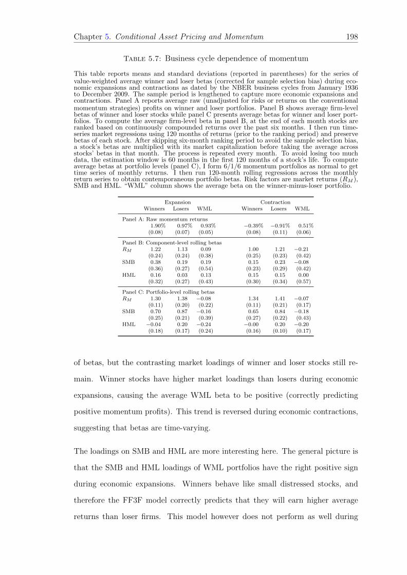
Chapter 5. Conditional Asset Pricing and Momentum 198
Table 5.7: Business cycle dependence of momentum
This table reports means and standard deviations (reported in parentheses) for the series ofvalue-weighted average winner and loser betas (corrected for sample selection bias) during eco-nomic expansions and contractions as dated by the NBER business cycles from January 1936to December 2009. The sample period is lengthened to capture more economic expansions andcontractions. Panel A reports average raw (unadjusted for risks or returns on the conventionalmomentum strategies) profits on winner and loser portfolios. Panel B shows average firm-levelbetas of winner and loser stocks while panel C presents average betas for winner and loser port-folios. To compute the average firm-level beta in panel B, at the end of each month stocks areranked based on continuously compounded returns over the past six months. I then run time-series market regressions using 120 months of returns (prior to the ranking period) and preservebetas of each stock. After skipping six-month ranking period to avoid the sample selection bias,a stock’s betas are multiplied with its market capitalization before taking the average acrossstocks’ betas in that month. The process is repeated every month. To avoid losing too muchdata, the estimation window is 60 months in the first 120 months of a stock’s life. To computeaverage betas at portfolio levels (panel C), I form 6/1/6 momentum portfolios as normal to gettime series of monthly returns. I then run 120-month rolling regressions across the monthlyreturn series to obtain contemporaneous portfolio betas. Risk factors are market returns (RM ),SMB and HML. “WML” column shows the average beta on the winner-minus-loser portfolio.
Expansion ContractionWinners Losers WML Winners Losers WML
Panel A: Raw momentum returns1.90% 0.97% 0.93% −0.39% −0.91% 0.51%
(0.08) (0.07) (0.05) (0.08) (0.11) (0.06)
Panel B: Component-level rolling betasRM 1.22 1.13 0.09 1.00 1.21 −0.21
(0.24) (0.24) (0.38) (0.25) (0.23) (0.42)SMB 0.38 0.19 0.19 0.15 0.23 −0.08
(0.36) (0.27) (0.54) (0.23) (0.29) (0.42)HML 0.16 0.03 0.13 0.15 0.15 0.00
(0.32) (0.27) (0.43) (0.30) (0.34) (0.57)
Panel C: Portfolio-level rolling betasRM 1.30 1.38 −0.08 1.34 1.41 −0.07
(0.11) (0.20) (0.22) (0.11) (0.21) (0.17)SMB 0.70 0.87 −0.16 0.65 0.84 −0.18
(0.25) (0.21) (0.39) (0.27) (0.22) (0.43)HML −0.04 0.20 −0.24 −0.00 0.20 −0.20
(0.18) (0.17) (0.24) (0.16) (0.10) (0.17)
of betas, but the contrasting market loadings of winner and loser stocks still re-
main. Winner stocks have higher market loadings than losers during economic
expansions, causing the average WML beta to be positive (correctly predicting
positive momentum profits). This trend is reversed during economic contractions,
suggesting that betas are time-varying.
The loadings on SMB and HML are more interesting here. The general picture is
that the SMB and HML loadings of WML portfolios have the right positive sign
during economic expansions. Winners behave like small distressed stocks, and
therefore the FF3F model correctly predicts that they will earn higher average
returns than loser firms. This model however does not perform as well during

Chapter 5. Conditional Asset Pricing and Momentum 199
economic contractions, with the loading of WML portfolio on SMB and HML
factors are -0.08 and 0.00. Although these betas are negative and close to zero,
the fact that their magnitude is much lower than that estimated during economic
expansions correctly predicts that momentum portfolios are more profitable in up
markets. Another point is that all betas exhibit time variations as evidenced by
the contrasting changes in loadings of winner and loser stocks when the economy
switches from expansions to contractions. In short, applying the FF3F model on
individual stock returns can shed light on solving the puzzle of Fama and French
(1996).
Again, these results, which have not been documented before, are concealed when
the same asset pricing models are estimated on aggregate portfolio returns (Grundy
and Martin (2001) and Lewellen and Nagel (2006)). Panel C reports the average
of contemporaneous betas of winner/loser portfolios that are estimated by running
120-month rolling window regressions of monthly WML returns on the risk factors.
In general, the picture in panel B is reversed here. The high (favorable) loading on
the market risk of WML portfolios during economic expansions now disappears.
Average betas on SMB and HML also incorrectly predict negative momentum
profits in both states of the economy. Similar to Fama and French (1996), loser
portfolios load more on SMB and HML factors than winner portfolios, counter-
intuitively suggesting that losers should earn higher average returns than winners.
In other words, the puzzle of Fama and French (1996) is still unsolved when the
test is conducted on aggregate portfolio returns. Panel C also shows that although
both the CAPM and the FF3F model cannot predict momentum returns, the for-
mer model has a less negative market beta in both economic states, indicating
that Boguth et al. (2011) find evidence in favor of the conditional CAPM because
they estimate their models at portfolio levels.
These findings suggest that momentum may be an artifact of the way stocks are
selected in the portfolio. When stocks are grouped into portfolios the true degree

Chapter 5. Conditional Asset Pricing and Momentum 200
of time variations and the asymmetric behavior of winner and loser stocks are
hidden. Winner/loser portfolios’ betas, when estimated using monthly portfolio
returns, become less time-varying and act differently to those estimated using
returns on individual stocks. This leads us to suspect that momentum is a puzzle
not because we lack an asset pricing model to explain it, but because the myth
of momentum is obscured by the mechanical way of stock selections. The asset
pricing model is therefore more powerful when being examined on individual stock
components.
5.4.6 The sensitivity of sample selection bias
As described earlier, the primary difference between my methodology of component-
level risk adjustments and previous research is that I correct for the sample se-
lection bias by excluding ranking period returns from the estimation window. In
order to demonstrate the sensitivity of this bias, I now replicate Chordia and Shiv-
akumar (2002) and Wang and Wu (2011) whose results are reported in Table 5.8.
The methodology of this Table is similar to that of Table 5.5, except that the
estimation window is now the past 120 months of stock returns from t − 120 to
the end of the ranking period t− 1 (i.e., including the six-month ranking period).
Again, to avoid losing too much data, I employ 60-month window in the first 120
months of a stock’s life and the full 120-month window afterward.
Panel A of Table 5.8 reports results from unconditional models where Zt−1 do
not appear in the model (5.4) (no interaction terms). The unconditional firm-
level adjustment is employed in Wang and Wu (2011).25 Comparing with average
unconditional CAPM alpha of Table 5.5, we can see that the sample selection bias
does not affect the average alpha, which remains at 0.96% per month (t-statistic
= 4.96). The average alpha from the unconditional FF3F model however is badly
25Wang and Wu (2011) do not compare models but only test the unconditional FF3F model.

Chapter 5. Conditional Asset Pricing and Momentum 201
affected. The unconditional average FF3F alpha is 0.65% per month (t-statistic =
3.63), which is a 13bps reduction from that in Table 5.5. Thus, the bias reduces the
average risk-adjusted returns even when betas are not allowed to be time-varying.
Table 5.8: Component-level risk adjusted momentum returns, with sam-ple selection bias
This table reports average risk-adjusted returns on 6/1/6 momentum portfolios from January1963 to December 2009. 6/1/6 overlapping portfolios are constructed by ranking returns overthe past 6 months and skip one month before holding stocks for the next 6 months. The strategyis followed every month. In panel B, returns on each individual stock in the winner and loserportfolios are risk-adjusted using the following model:
radji,t = ri,t − rf −K∑j=1
(β>ijZt−1)f jt
where β>ij is estimated using the past 120-month returns from t-120 to t-1 (i.e. 120 monthsprior to the holding period). Factors, f jt, are the excess return on the market (RM ) or Famaand French three factors (FF3F). State variables, f jt, are dividend yield, term spread and thedefault spread. Panel A reports risk-adjusted returns that are similarly computed as in panelB, except that the model does not have interaction terms (or f jt). Returns are reported inpercentages. WML is the returns on winner − loser portfolios. Panel C shows the adjustedreturns from macroeconomic model of Chordia and Shivakumar (2002), which includes threestate variables and the yield on three-month T-bills and a January dummy (without risk factors,f jt). t-statistics from the method outlined in Cochrane (2005) are reported in parentheses; theadjustment factor is calculated using formula (5.5). ∗, ∗∗, ∗ ∗ ∗ represent the significance levelsat 10%, 5% and 1%, respectively. Stocks are required to have at least 24 months of valid returnsover the past 60 months to be ranked. The estimation window is 60 months in the first 120months of a stock’s life, afterward the window is extended to 120 months.
Models Winners Losers WML
Panel A: Unconditional risk adjustmentCAPM 0.54 −0.42 0.96
(3.58)∗∗∗ (−2.51)∗ (4.96)∗∗∗
FF3F 0.1986 −0.45 0.65(1.70)∗ (−3.70)∗∗∗ (3.63)∗∗∗
Panel B: Time-varying risk adjustmentCAPM 0.42 −0.19 0.61
(2.24)∗∗ (−1.03) (2.46)∗∗
FF3F −0.29 0.01 −0.29(−1.45) (0.01) (−0.87)
Panel C: Chordia and Shivakumar’s (2002) conditional macroeconomic adjustmentMacro variables −10.79 −7.82 −2.97
(−7.91)∗∗∗ (−6.79)∗∗∗ (−1.52)Macro and Jan −12.79 −9.34 −3.45
(−2.42)∗∗ (−2.07)∗∗ (−1.63)
Panel B reports risk-adjusted returns from the full conditional model (5.4). The
first row of panel B reports the average time-varying risk-adjusted return at the
individual stock level using the conditional CAPM. The conditional CAPM per-
forms exceptionally well by reducing the average alpha to 0.61% per month with

Chapter 5. Conditional Asset Pricing and Momentum 202
a t-statistic of 2.46, statistically significant at the 5% level. The conditional FF3F
model is even more aggressive in reversing the momentum effect, with the aver-
age alpha being −0.29% per month (t-statistic = −0.86), statistically insignificant
even at the 10% level. These findings indicate that the bias causes the conditional
risk adjustment at component levels to explain all momentum returns.
Panel C shows the average adjusted returns from the macroeconomic model of
Chordia and Shivakumar (2002). Consistent with their study, panel C shows that
their models can also make momentum returns disappear. The average adjusted
momentum return using Equation (5.7) is −2.97% per month, which is econom-
ically significant although t-statistic is only −1.52. Adding the January dummy
makes the adjusted return even more negative with −3.45% per month (t-statistic
= −1.63).
5.4.7 Sensitivity analysis: expanding-window estimation
This subsection provides a robustness test on whether the component-level risk
adjustment is sensitive to expanding-window estimations. Specifically, I estimate
the conditional models using each component i’s returns over an extending window,
starting from the first month of stock’s returns to the month prior to the ranking
period. This sensitivity test is motivated by Fama and French (1992), Ferson
and Harvey (1999), Lettau and Ludvigson (2001), and Liu and Zhang (2008) who
endorse the use of extending windows, which arguably produces more accurate
estimations due to having more data.
Table 5.9 shows the average component-level alpha estimated similar to Table 5.5,
but with extending windows. My conclusions do not change. Panel A reports
the average alpha from unconditional models. These alphas are not economically
different from those of Table 5.5. The average alpha from the unconditional FF3F

Chapter 5. Conditional Asset Pricing and Momentum 203
Table 5.9: Component-level risk-adjusted momentum returns, expanding-window estimation
This table reports average risk-adjusted returns on 6/1/6 momentum portfolios from January1963 to December 2009. 6/1/6 overlapping portfolios are constructed by ranking returns overthe past 6 months and then skip one month before holding stocks for the next 6 months. Thestrategy is followed every month. In panel B, returns on each individual stock in the winner andloser portfolios are risk-adjusted using the following model:
radji,t = ri,t − rf −K∑j=1
(β>ijZt−1)f jt
where βTij is estimated using returns over an extending window, starting from the first month
to the month prior to the ranking period (i.e, ranking period returns are not included in theestimation). Risk factors, fjt, are excess returns on the market (RM ) or Fama and Frenchthree factors (FF3F). State variables, Zt−1, are dividend yield, term spread and the defaultspread. Panel A reports risk-adjusted returns that are similarly computed as in panel B, exceptthat the unconditional model does not have interaction terms (without Zt−1). Returns arereported in percentages. WML is the return on winner − loser portfolios. Panel C showsaverage adjusted returns from macroeconomic model of Chordia and Shivakumar (2002), whichincludes the three IVs in this study and the yield on three-month T-bills and a January dummy(without risk factors, fjt). t-statistics from the method outlined in Cochrane (2005) are reportedin parentheses; the adjustment factor is calculated using formula (5.5). ∗, ∗∗, ∗ ∗ ∗ represent thesignificance levels at 10%, 5% and 1%, respectively.
Models Winners Losers WML
Panel A: Unconditional risk adjustmentCAPM 0.53 −0.44 0.97
(3.47)∗∗∗ (−2.62) (4.79)∗∗∗
FF3F 0.30 −0.50 0.80(3.13)∗ (−3.76) (4.55)∗∗
Panel B: Time-varying risk adjustmentCAPM 0.66 −0.25 0.91
(3.85)∗ (−1.34) (4.13)∗∗∗
FF3F 0.20 −0.45 0.65(0.96)∗ (−2.87) (2.35)∗∗
Panel C: Chordia and Shivakumar’s (2002) conditional macroeconomic adjustmentMacro variables −4.91 −9.52 4.61
(−1.96)∗ (−3.41) (2.23)∗∗
Macro and Jan −7.41 −11.09 3.68(−3.01)∗ (−4.08) (1.69)∗
is 0.80% per month (t-statistic = 4.55), compared with the 0.78% per month (t-
statistic = 4.46) of 120-month windows in Table 5.5. Similarly, Panel B shows
that the conditional FF3F model also performs well in terms of reducing the
average alpha, with 0.65% per month (t-statistic = 2.35), statistically significant
at the 5% level. This represents a 45% reduction over the corresponding portfolio-
level estimate (Table 5.2). Finally, the average adjusted return from Chordia and
Shivakumar’s (2002) macroeconomic models is still highly positive, suggesting that
this model is sensitive to the correction of sample selection bias.

Chapter 5. Conditional Asset Pricing and Momentum 204
In short, this subsection has shown that my findings still hold under the expanding-
window estimation. It reconfirms that the correction for sample selection bias is
crucial and that the conditional FF3F model performs much better when being
applied on the individual component of momentum portfolios.
5.4.8 Sensitivity analysis: Fama and French (1996) mo-
mentum portfolios
This subsection tests whether my main results still hold under a different construc-
tion of momentum portfolios. In particular, I examine the momentum portfolio
of Fama and French (1996) in which stocks are ranked based on their continu-
ously compounded returns over the past year, and the portfolio is held for one
month with one-month skipping period in between. Although I can confirm the
robustness of my findings in other strategy formations of Jegadeesh and Titman
(1993), I report the results for Fama and French’s (1996) portfolios to be consis-
tent with Fama and French (1996) and many subsequent papers (e.g., Grundy and
Martin (2001) and Asness et al. (2013)). Because these strategies have one-month
holding period, they are rebalanced more frequently and therefore I expect that
conditional asset pricing models are more powerful when being applied on indi-
vidual components’ returns. Again, this high explanatory power comes from its
ability to account for the frequent change in portfolio compositions and weights
of the portfolio’s components.
Table 5.10 reports average risk-adjusted returns, which are computed similarly as
in Table 5.5. Panel A shows the results from unconditional models in which state
variables are not included in the regression. We can see that both the unconditional
CAPM and FF3F model cannot explain momentum returns. The average alpha
from the CAPM is 1.19% per month (t-statistic = 4.85) while the FF3F model

Chapter 5. Conditional Asset Pricing and Momentum 205
has the average alpha of 0.95% per month (t-statistic=4.37); both of them are
statistically significant at the 1% level.
Table 5.10: Component-level risk-adjusted returns on Fama and French(1996) momentum portfolios
This table reports average risk-adjusted returns on Fama and French’s (1996) momentum port-folios from January 1963 to December 2009. Momentum portfolios are constructed by rankingstock returns over the past one year months and then skip one month before holding stocksfor the next one months. The strategy is followed every month. In panel B, returns on eachindividual stock in the winner and loser portfolios are risk-adjusted using the following model:
radji,t = ri,t − rf −K∑j=1
(β>ijZt−1)f jt
where β>ij is estimated using 120-month returns prior to the ranking period (i.e, ranking periodreturns are not included in the estimation). In order to avoid losing too much data, I use60-month windows of returns in the first 120 months and then use the full 120-month windowafter that. Risk factors, f jt, are excess returns on the market (RM ) or Fama and Frenchthree factors (FF3F). State variables, Zt−1, are dividend yield, term spread and the defaultspread. Panel A reports risk-adjusted returns that are similarly computed as in panel B, exceptthat the unconditional model does not have interaction terms (without Zt−1,). Returns arereported in percentages. WML is the return on winner − loser portfolios. Panel C showsaverage adjusted returns from macroeconomic model of Chordia and Shivakumar (2002), whichincludes the three IVs in this study and the yield on three-month T-bills and a January dummy(without risk factors, f jt). t-statistics from the method outlined in Cochrane (2005) are reportedin parentheses; the adjustment factor is calculated using formula (5.5). ∗, ∗∗, ∗ ∗ ∗ represent thesignificance levels at 10%, 5% and 1%, respectively.
Models Winners Losers WML
Panel A: Unconditional risk adjustmentCAPM 0.70 −0.49 1.19
(4.04)∗∗∗ (−2.73)∗∗∗ (4.85)∗∗∗
FF3F 0.40 −0.55 0.95(3.43)∗∗∗ (−3.86)∗∗∗ (4.37)∗∗∗
Panel B: Time-varying risk adjustmentCAPM 0.78 −0.18 0.96
(3.65)∗∗∗ (−0.83) (3.10)∗∗∗
FF3F 0.12 −0.26 0.38(0.40) (−1.02) (0.77)
Panel C: Chordia and Shivakumar’s (2002) conditional macroeconomic adjustmentMacro variables −4.35 −9.38 5.03
(−1.47) (−3.12)∗∗∗∗ (1.75)∗
Macro and Jan −7.31 −11.07 3.76(−2.47)∗∗ (−3.73)∗∗∗ (1.26)
Panel B shows average alphas from conditional models. We see a better picture
here where the conditional CAPM yields the average risk-adjusted return of 0.96%
per month (t-statistic = 3.10), statistically significant at the 1% level. The con-
ditional FF3F model performs exceptionally well by reducing the average alpha
to only 0.38% per month (t-statistic = 0.77), statistically insignificant even at
the 10% level. This reduction is also economically large with 60% down from the

Chapter 5. Conditional Asset Pricing and Momentum 206
conditional CAPM. These findings confirm my conjecture that, as the Fama and
French’s (1996) momentum portfolios involve frequent rebalancing and changes
in the weight of individual stocks, the component-level risk adjustment from the
FF3F model can correctly account for the time variation of individual compo-
nents’ betas, which are not seen on the aggregate portfolio return. Finally, panel
C shows average returns from Chordia and Shivakumar’s (2002) macroeconomic
model. Consistent with the earlier findings that, once I correct for the sample
selection bias, the average WML return becomes economically positive, ranging
from 3.76% per month to 5.03% per month although they are still statistically
insignificant.
In short, this subsection has shown that my findings also hold for the popular
momentum portfolio of Fama and French (1996). Fama and French (1996) find
that their FF3F model inflates the momentum alpha rather than reducing it when
being applied on aggregate portfolio returns. Using the same momentum portfolio
construction, I find empirical support for their multifactor model. The conditional
FF3F model performs very well by reducing the average alpha to 0.38% per month,
representing a 60% reduction from the conditional CAPM estimate.
5.5 Conclusion
I argue that the momentum effect is an artifact of the way stocks are selected
into portfolios. Particularly, stocks are picked in such a way that their true time-
varying dynamics are concealed on aggregate portfolio returns. Motivated by
this observation, I show that the puzzle of Fama and French (1996) is solved at
the individual winner and loser stock (component) level. Winner stocks, which
act more like small and distressed firms, load more on the SMB and HML factors.
Therefore, winners should earn higher future average returns and losers should earn
lower average returns, causing positive expected momentum profits. I pick two of
Chapter 5. Conditional Asset Pricing and Momentum 207
the most popular momentum portfolios in the literature to report my results. The
first one is the 6/1/6 momentum portfolio of Jegadeesh and Titman (1993). I find
that the conditional FF3F, when being used to risk adjust returns on individual
stocks (components) of the portfolio, reduces the average alpha to 0.61% per month
(t-statistic = 2.13), representing a 50% decrease from the portfolio-level estimate.
The second portfolio is consistent with Fama and French (1996), which has only
one-month holding periods. Because the component-level risk adjustment can
correctly account for the frequent change in weights and portfolio’s compositions,
the conditional FF3F model performs exceptionally well with the average alpha of
0.38% (t-statistic = 0.77), statistically insignificant even at the 10% level.
I point out the sample selection bias in the component-level risk adjustment of
existing studies in which winner and loser betas are biased due to the inclusion
of ranking period returns in the estimation. Because of this bias, all asset pricing
models that account for time-varying risks can completely explain momentum
returns and the macroeconomic model of Chordia and Shivakumar (2002) can
even make momentum payoffs become negative. I propose a simple correction of
this bias by excluding the ranking period returns from the estimation. With the
bias correction, the negative adjusted momentum returns (ranging from -2.97%
to -3.45% per month) in Chordia and Shivakumar (2002) become economically
positive ranging from 3.76% to 5.03% per month.
5.A Derivations of alpha decomposition in mul-
tifactor models
Consider a multi-factor pricing model
rit = f ′t · βit + eit

Chapter 5. Conditional Asset Pricing and Momentum 208
where f t = µt+ut and βit = βi+ηit and E(ηit) = 0 and is likely to be positively
serially correlated. Consider estimating the unconditional version of the CAPM,
with
θT =
(1
T
T∑t=1
X tX′t
)−1
1
T
T∑t=1
X trit
where
θ =
αUβU
and X t = (1,f ′t)
′. Under quite general regulatory conditions we have
plimθT = Q−1plim1
T
T∑t=1
X trit
where
Q = plim1
T
T∑i=1
X tX′t =
1 µ′f
µf Σf + µfµ′f
and using the partitioned matrix inverse formula we have
Q−1 =
1 + µ′fΣ−1f µf −µ′fΣ
−1f
−Σ−1f µf Σ−1
f
.
Note that
plim1
T
T∑t=1
X trit = plim1
T
T∑t=1
X t(f′tβi + f ′tηi,t + εi,t)
= plim1
T
T∑t=1
f ′t
f tf′t
︸ ︷︷ ︸
=
µ′f
Σf + µfµ′f
βi + plim1
T
T∑t=1
f ′tηi,t
f tf′tηi,t
+ plim1
T
T∑t=1
X tεi,t︸ ︷︷ ︸=0

Chapter 5. Conditional Asset Pricing and Momentum 209
So we then have
plimθT −
0
βi
= Q−1plim1
T
T∑t=1
f ′tηi,t
f tf′tηi,t
and in particular
plimαT = (1 + µ′fΣ−1f µf )E(f ′tηi,t)− µ′fΣ−1
f E(f tf′tηi,t)
= E(f ′tηi,t)− µ′fΣ−1f cov(f t,f
′tηi,t) (5.10)
where E(f ′tηi,t) = plim 1T
∑Tt=1 f
′tηi,t and E(f tf
′tηi,t) = plim 1
T
∑Tt=1 f tf
′tηi,t are
consistent estimators of the relevant expectations.

Chapter 6
Conditional Asset Pricing, Value,
and Momentum in International
Equity Markets
This paper finds that using conditional asset pricing models to risk adjust returns
on individual stocks can help to explain momentum, value, and Asness et al.’s
(2013) COMBO anomalies in North America, Europe, Japan, and Asia Pacific. I
test the explanatory power of three competing models and find that the conditional
Fama and French (1993) three-factor (FF3F) model is the best performer in North
America, Japan, and Asia Pacific while the four-factor model (FF3F and the
coskewness risk factor) has the lowest average alpha in Europe. By applying asset
pricing models on the individual component of the portfolio, this study also offers
a new perspective to the debate of whether asset pricing is integrated across the
four regions. The results show that global risk factors are more successful than
their local counterparts in explaining anomalies in North America, Japan, and
Asia. All models, nevertheless, cannot fully rationalize each of the anomalies.
210

Chapter 6. Conditional Asset Pricing, Value, and Momentum in InternationalEquity Markets 211
6.1 Introduction
Jegadeesh and Titman (1993) document the profitability of momentum investing
strategies that exploit historical trends in stock prices by buying winner stocks,
those stocks that perform well over the past year, and simultaneously short selling
losers, those stocks that earned the worst returns over the same period. There is
also evidence that value stocks (those with high book-to-market ratios) outperform
growth stocks (those with low book-to-market ratios).1 These anomalies are not
specific to the U.S. market. Rouwenhorst (1998), Griffin et al. (2003), and Chui
et al. (2010) document the profitability of momentum strategies in international
equity markets. Fama and French (1998), Karolyi and Wu (2012), and Fama
and French (2012) find that the value premium is also persasive in international
markets.
While the literature is still in search of an asset pricing theory to explain momen-
tum and value effects, Asness, Moskowitz, and Pedersen (2013) (henceforth, AMP)
document that a COMBO strategy that equally invests in momentum and value
portfolios yields even more persistent and stable average returns and importantly
has a higher Sharpe ratio in the U.S, Japan, and European markets. This strategy
is also profitable in Japan where the average return on the momentum portfolio
is insignificant.
The general approach to testing asset pricing models is to apply them on the
aggregate portfolio returns. However, recent development in asset pricing tests has
shown that, for strategies that require frequent rebalancing such as the momentum
strategy, asset pricing models are more powerful if the time variation of individual
stocks’ betas is explicitly incorporated into the test.
1Early studies that document this value anomaly include Stattman (1980), Rosenberg et al.(1985), and Fama and French (1992)

Chapter 6. Conditional Asset Pricing, Value, and Momentum in InternationalEquity Markets 212
Boguth, Carlson, Fisher, and Simutin (2011) find that when the CAPM is con-
ditioned based on contemporaneous realized betas of individual winner and loser
stocks, the average momentum alpha declines by 20% to 40% relative to the un-
conditional measure. Chordia and Shivakumar (2002) employ a macroeconomic
model to adjust for returns of individual stocks of the momentum portfolio. They
find that momentum payoffs are strongly related to business cycles as dated by
the NBER and consequently suggest that momentum returns can potentially be
explained by time-varying expected returns.2 Wang and Wu (2011) show that em-
ploying the unconditional FF3F model to risk adjust returns on individual stock
components can reduce the average alpha by approximately 40%. In a similar
vein, the previous Chapter builds on this methodology by allowing stocks’ betas
to be time-varying, and more importantly, points out and corrects the sample
selection bias in the estimation. The Chapter shows that the conditional Fama
and French’s (1993) (FF3F) model, after correcting for the bias, can reduce the
average momentum alpha by 50%.3
This study has two goals. The first goal is to provide an international examination
of the component-level risk adjustment in four regions namely North America,
Europe, Japan, and Asia Pacific (23 developed countries). Most international
studies of value and momentum effects focus on the portfolio-level risk adjustment,
which, as pointed out in the previous Chapter, does not describe the true time
variation of individual stocks’ betas.
2They essentially employ two methods; the first is similar to this study’s (but do not accountfor sample selection biases) and the second is a two-way dependent portfolio sort between rawand predicted returns. Using the second method, Griffin et al. (2003) show that the findingsof Chordia and Shivakumar (2002) do not hold in 16 international markets. Similarly, Cooperet al. (2004) find that Chordia and Shivakumar’s (2002) results from the two-way portfolio sortsare driven by market microstructure biases of penny stocks. Finally, the Chapter 5 of this thesisshows that the first method of Chordia and Shivakumar (2002) also suffers from ‘sample selectionbias’. When I correct for this bias, the average adjusted return from Chordia and Shivakumar’s(2002) models reverses from -2.97% per month to 5.03% per month.
3As argued in the previous Chapter and Chordia et al. (2011), testing asset pricing modelsat the component level helps avoid the critique of Lo and MacKinlay (1990a) and Lewellen et al.(2010) that particular methods of sorting stocks can significantly affect the final results. Anget al. (2010) change the conventional view by showing that standard errors from cross-sectionalregressions at firm levels are not higher than at the portfolio level.

Chapter 6. Conditional Asset Pricing, Value, and Momentum in InternationalEquity Markets 213
This study is also the first to examine the explanatory power of Harvey and
Siddique’s (2000) conditional coskewness risk factor on momentum, value and
COMBO portfolios in 23 developed markets. Although Harvey and Siddique
(2000) construct their factor using rolling-window regressions, their estimations
do not allow for the time variation in the parameters, and thus they essentially
test unconditional models. Even though asset pricing models perform uncondi-
tionally well, the conditional version may behave differently (Ferson and Harvey,
1999). Therefore, my next aim is to investigate the coskewness factor under condi-
tioning information. This test also helps examine whether the explanatory power
of FF3F is subsumed once the coskewness risk is accounted for.
The second goal is to investigate whether international markets are integrated.4
As in Fama and French (2012), I examine this question by comparing the average
alpha from the model of global risk factors and that of local risk factors. The cur-
rent evidence on market integration is mixed. Fama and French (2012) show that
unconditional local risk factors have higher explanatory power than global coun-
terparts in explaining local returns – suggesting that markets are not integrated.
However, Karolyi and Wu (2012) show that when they control for the fact that
stocks being cross-listed in more than two national markets are more integrated
to the world market, their hybrid global model achieves lower pricing errors than
local versions.
My findings are easily summarized. Firstly, when global risk factors are used to
risk adjust returns of the individual component of momentum, value, and COMBO
portfolios, I confirm the U.S. findings in Chapter 5 that the component-level risk
adjustment can help reduce the average alpha of global and regional portfolios.
Compared to the portfolio-level estimate, the average component-level alpha is
lower by up to 50%. Although details vary, the global conditional four-factor
4The question is important in finance because it will help us determine which discount rateshould be used in international capital budgeting. Moreover, mutual funds that hold interna-tional stocks also need an appropriate asset pricing model to ‘price’ the risk of their portfolios.

Chapter 6. Conditional Asset Pricing, Value, and Momentum in InternationalEquity Markets 214
model (i.e., the FF3F and the coskewness factor) tends to be the best performer
in Europe while the global conditional FF3F model has the lowest average risk-
adjusted return in North America, Japan, and Asia Pacific. Secondly, when being
applied on individual components, global risk factors are more powerful than their
local counterparts in explaining both global and regional anomalies – in contrast
to the portfolio-level evidence. I find that, based on the reduction in average risk-
adjusted returns, markets in North America, Japan, and Asia are more integrated
to the global market. Except for Europe where we should use local risk factors to
explain local stock returns, global risk factors produce lower average pricing errors
than their local counterparts everywhere.
I argue that the success of component-level risk adjustment comes from its ability
to pick up the time-varying global integration of some stock components that
tests based on the aggregate portfolio return can not detect. As I review prior
studies in the next section, this study is different from previous research in terms
of the methodology. Existing studies (e.g., Fama and French (2012)) generally test
unconditional models while I allow betas to be time-varying. This time variation is
crucial in light of Bekaert and Harvey (1995) who argue that the degree of market
integration can change over time. By allowing conditionally expected returns on
local markets to be determined by their covariance with the global market return
as well as by the variance of country returns, Bekaert and Harvey (1995) find that
many markets are conditionally integrated while some countries are becoming less
integrated to the global market. Moreover, rather than using conditional models
to risk adjust aggregate portfolio returns, I employ them to adjust for the risk
of individual components. This method hence accounts for the fact that some
stocks such as those of large global firms are more integrated to the global market
than small stocks, as pointed out by Karolyi and Stulz (2003) and Karolyi and
Wu (2012). Consequently, the component-level risk adjustment allows global asset
pricing models to have the highest explanatory power on the returns of stocks that

Chapter 6. Conditional Asset Pricing, Value, and Momentum in InternationalEquity Markets 215
are more globally integrated. Portfolio-level tests however treat all firms in the
same way and hence ignore this heterogeneity among the stock components. In
fact, my conclusion is consistent with Bekaert and Harvey (1995) and Karolyi and
Wu (2012) that global risk factors are more powerful in pricing both global and
regional returns than their local counterparts.5
The study proceeds as follows. The next section reviews the theory as well as
primary literature on which I build this study. Section 6.3 discusses sources of
data and confirms previous studies on the portfolio-level evidence. I report the
main findings in Section 6.4 where I employ the methodology of component-level
risk adjustment similar to the previous Chapter. Section 6.5 concludes this study.
6.2 Theory and related literature
This study contributes to the literature that tests the explanatory power of as-
set pricing models in international markets. In performing this test, apart from
trying to investigate whether some common risk factors such as the market risk,
size, and book-to-market risk factors of Fama and French (1993) can rationalize
international stock returns, researchers also encounter the question of whether the
local or global version of those risks matter.
Theoretically, international asset pricing theory predicts that the risk premium of
an asset is determined by its covariance risk with the world market portfolio (i.e.,
global market risks). To see this, I review the theoretical framework of Grauer
et al. (1976), Stulz (1995), and Karolyi and Stulz (2003) who consider a model in
the perfect capital market where there are no transportation costs, no tariffs, no
taxes, no transaction costs, and no restrictions to short sales. There is also only
5Griffin et al. (2010), who test the market efficiency in international exchanges, also arguethat “an advantage of using individual stocks is that one can allow correlations to switch signacross stocks.”

Chapter 6. Conditional Asset Pricing, Value, and Momentum in InternationalEquity Markets 216
one consumption good and the law of one price holds so that the purchasing power
parity is maintained.
They next consider a one-period economy in which the expected return on a do-
mestic asset is expressed in the form of Sharpe (1964) and Lintner (1965) domestic
CAPM and there is only one risk-free asset earning rf :
E(ri)− rf = αi + βLi [E(rL)− r] + εLi (6.1)
where E(ri) is the expected return on asset i, E(rL) denotes the expected return
on the local market portfolio, βLi = Cov(ri,rL)V ar(rL)
is the local beta of asset i. If foreign
investors were not allowed to hold domestic assets, Equation (6.1) can be used
and αi is expected to be equal to zero. However, in the real world where foreign
investors have access to domestic assets, the local CAPM is no longer appropriate
and only the global market risk should matter such that the global CAPM holds.
E(ri)− rf = αi + βGi [E(rG)− r] + εGi (6.2)
where E(rG) is the expected return on the global market portfolio and βGi =
Cov(ri,rG)V ar(rG)
is the global beta of asset i.
Karolyi and Stulz (2003) show that if we employ the local CAPM to explain local
stock returns while the global CAPM should be used, Equations (6.1) and (6.2)
imply that the pricing error is:
αi = [βGi − βGL βLi ][E(rG − rf )] (6.3)
where βGL is the global beta of the domestic market, which is found by running the
global market model regression:
E(rL)− rf = αL + βGL [E(rG)− r] + εGL (6.4)

Chapter 6. Conditional Asset Pricing, Value, and Momentum in InternationalEquity Markets 217
By substituting Equation (6.4) into Equation (6.1), we get the global market beta
of asset i:
βGi = βLi βGL +
Cov(εLi , rG)
V ar(rG)(6.5)
Substituting Equation (6.5) into Equation (6.3) to get the pricing mistake from
using the local CAPM when the global CAPM is right:
αi =Cov(εLi , rG)
V ar(rG)[E(rG)− rf ] (6.6)
Equation (6.6) indicates that as long as the local market model residual is cor-
related with the global market return, the domestic CAPM will incorrectly price
the local asset return. This mistake can easily be seen if we look at large global
firms whose returns are correlated with international market portfolios and the
domestic market risk cannot account for all systematic risks. On the other hand,
the pricing error in Equation (6.6) may not be a big concern for small domestic
stocks whose εLi is not highly correlated with the global market. Consequently,
this theory also motivates the methodology employed in this Chapter, which takes
into account the global market integration of individual stocks.
Empirically, the literature on market integration has been mixed. Griffin (2002)
examines whether the Fama and French’s (1993) three-factor model (FF3F) (mar-
ket risks, size premium, and book-to-market risk premium) are priced in four
countries, namely the U.S., U.K., Canada, and Japan. He finds that local mod-
els have lower average pricing errors than global models. Of note is that Griffin
(2002) also tests the model on individual stock returns. However, he does not
allow for the time variation in betas that in turn account for the time-varying
market integration of individual stocks (as argued by Bekaert and Harvey (1995)),
and also does not test the FF3F model on momentum effects. The scope of this

Chapter 6. Conditional Asset Pricing, Value, and Momentum in InternationalEquity Markets 218
Chapter is also larger as I employ a set of common asset pricing models to explain
momentum, value, and COMBO effects in 23 equity markets.
Bekaert and Harvey (1995) allow conditionally expected returns on local markets
to be determined by their covariance with the global market return as well as
by the variance of country returns, and find that many markets are conditionally
integrated. They also argue that markets that allow stocks to be cross-listed
are more integrated. More recently, Rapach et al. (2013) examine the lead-lag
relationship of stock returns among industrialized markets and find that lagged
U.S. returns have a significant predictive power of returns in non-U.S. countries.
In contrast, lagged non-U.S. returns cannot predict U.S. stock returns, suggesting
the important role of U.S. market in driving global market integration. These
studies together point to a conjecture that markets can be integrated and the
global risk factors are more powerful if we account for the time-varying market
integration at individual stock levels. In particular, we should expect that North
American markets are more integrated to the global market.
Recent literature also focuses on various variants of multifactor asset pricing mod-
els, and arrives at different conclusions. Fama and French (1998) find that a global
two-factor model including the global market return and the global spread of high
over low book-to-market portfolios can produce better descriptions of international
value returns. Fama and French (2012), on the other hand, show that the local
version of their FF3F model (especially in Asia and Europe) can better capture
the local size, value, and momentum returns, suggesting that international mar-
kets are not integrated. Karolyi and Wu (2012) examine another variant of the
global FF3F that includes a set of FF3F constructed using firms whose shares are
cross-listed in an overseas market and another set of FF3F constructed using firms
whose shares are not cross-listed. They show that their ‘hybrid’ multifactor model
can explain well both global and local stock returns, indicating that international
markets are in fact integrated. In a similar vein, Asness et al. (2013) (AMP) show

Chapter 6. Conditional Asset Pricing, Value, and Momentum in InternationalEquity Markets 219
that global market, value and momentum factors that are constructed using all
asset classes (not just equities) can better explain the local value and momentum
returns in the U.S. than the commonly used U.S. FF3F model – again pointing to
some common factors driving global returns.
The common methodology in those studies is that they examine variants of the
well-known FF3F model in the U.S. on the aggregate local portfolio and therefore
the question of whether the original FF3F model, which is empirically motivated
in the U.S., can describe international stock returns is still under-explored. In this
study, I do not augment the original FF3F model and, different from the previous
research, I allow betas to be time-varying at the component level. Consequently,
this methodology accounts for the fact that some stocks (components) are con-
ditionally integrated to the global market while other stocks in the portfolio are
not.
6.3 Data and summary statistics
I collect international stocks returns and accounting data from Thomson Reuters
Tick History (TRTH) and WorldScope between November 1989 and December
2011.6 The relatively recent sample period is chosen to have the most comprehen-
sive coverage of WorldScope database and also consistent with Fama and French
(2012), who source similar data from Datastream, WorldScope and Bloomberg be-
tween January 1989 and March 2011. Following the literature (e.g., Griffin et al.
(2003) and Griffin et al. (2005)), I source local data from local databases if they
are available. Specifically, U.S. monthly stock returns (for NYSE, Amex and Nas-
daq) and accounting data are collected from CRSP and Compustat, respectively.
Similar data for Australian companies are also separately collected from CRIF
6TRTH is supplied by SIRCA. As TRTH data starts from January 1996, I obtain internationalmarket data before 1996 from WorldScope.

Chapter 6. Conditional Asset Pricing, Value, and Momentum in InternationalEquity Markets 220
(Center for Research in Finance) supplied by the University of New South Wales
and MorningStar’s Aspect databases, respectively.
To maintain a large number of stocks in each portfolio, I follow Fama and French
(2012) and group stocks into four regions: (i) North America (NA), which consists
of the United States (U.S.) and Canada; (ii) Japan; (iii) Asia Pacific, including
Australia, New Zealand, Hong Kong and Singapore (but not Japan); and finally
(iv) Europe, including Austria, Belgium, Denmark, Finland, France, Germany,
Greece, Ireland, Italy, the Netherlands, Norway, Portugal, Spain, Sweden, Switzer-
land, and the United Kingdom. The purpose of these market combinations are
parsimony as well as maintaining a certain degree of market integration. The U.S.
and Canadian markets are the most integrated and can be treated as one market.
Similarly, most European countries are members of the European Union (EU),
which undoubtedly enjoy the benefit of market integration. As noted in Fama and
French (2012), the most segmented region is Asia Pacific, which may reduce the
power of portfolio tests.
I collect all available stocks from each country that are non-financial.7 Consistent
with the literature (e.g., Ince and Porter (2006), Griffin et al. (2010) and Karolyi
and Wu (2012)), all returns are calculated in U.S. dollar terms and monthly returns
are set to missing if they are greater than 300% and then reversed in the following
month. Specifically, if either rt or rt−1 is greater than 300% and (1 + rt−1)(1 +
rt) − 1 ≤ 50%, then both rt−1 and rt are treated as missing values. In order to
7For U.S. stocks, I choose the share codes of 10 and 11 in the CRSP database. For Australianstocks, I limit the “security type” field to “ordinary”. For other non-U.S. stocks, I follow Griffinet al. (2010) and Hou et al. (2011), who employ Datastream database, to scan stocks’ names andexclude those containing “REIT”, “REAL ESTATE”, “REAL EST”, “GDR”, “GDR”, “PF”,“PREF”, “PRF”, “ADS”, “CERTIFICATES”, “RESPT”, “RIGHT”, “PAID IN”, “UNIT”, “IN-COME FD”, “INCOME FUND”, “HIGH INCOME”, “INC GROWTH”, “INC GW”, “UTS”,“RTS”, “CAP.SHS”, “SBVTG”, “STG”, “GW.SD”, “RTN.INC”, “VTC”, “ORTF”, “YIELD”,“GUERNSEY”, “DUPLICATE”, “DUAL PURPOSE”, “NOT RANK”, “DIVIDEND”, “VOT-ING”, “NV”, “PR PB”, “NRFD”, “FBDEAD” “GSH”, “CONV”, “SR SER”, “VVPR STRIP”,“EXH EXCHANGEABLE”, “SPLIT”, “USE”, “VXX CSE”, “PV”, “RP”, “CERT”, “CERTS”,“PC”, “VXX”, “GENUSSCHEINE”, “RNC RIGHTS”, “ADP”, “CIP”, “ORA”.
Chapter 6. Conditional Asset Pricing, Value, and Momentum in InternationalEquity Markets 221
construct value portfolios, stocks are also required to have available book values
(WordScope data item: WC05476) to be included in the final sample.
Following AMP’s study, the book-to-market (BM) ratio is computed as lagged 6-
month book value (to ensure that the information is available to investors) over the
current market price. Fama and French (1993, 2012) however use 12-to-24-month
lagged book value and only update the market value once a year (this can be in
the same month with book value). I follow AMP because one objective of this
study is to explain their newly documented COMBO anomaly. They find that the
most recent BM ratio can produce more negative correlations between momentum
and value effects. I find consistent results, reported in later subsections, and my
value returns are comparable to theirs.
The final sample on average contains 17,375 stocks per month from 23 developed
markets. In terms of the number of stocks, North America, Europe, Japan and
Asia Pacific account for 39.11%, 25.43%, 18.97% and 16.48% total number of
stocks in the global sample, respectively. North America is also the largest mar-
ket, accounting for 43.48% of the total global market capitalization. Europe is the
second largest region with 35.22% of the global market capitalization. Asia Pa-
cific countries are much smaller with only 5.76%, compared with the stand-alone
Japan’s 15.54% portion of the global market capitalization. These statistics are
comparable with those of Fama and French (2012) and Karolyi and Wu (2012).
6.3.1 Risk factors
To maintain the comparability of my study with prior research, I obtain Fama
and French’s (1993) three factors, namely excess market returns (mkt), SMB and
HML, for each of the regions as well as global stock returns from Ken French’s

Chapter 6. Conditional Asset Pricing, Value, and Momentum in InternationalEquity Markets 222
website.8 As I am interested in testing conditional asset pricing models, I employ
three conditioning variables that are common in the literature (Fama and French,
1989). I use MSCI (global and regional) dividend yields, U.S. term spread (TERM)
computed as the difference in yields between ten-year and three-month yield spread
in the U.S. Treasury market; and the U.S. default spread (DEF), which is the
difference in yields between U.S. Baa- and Aaa- rated bonds.
Data on U.S. conditioning variables is obtained from Amit Goyal’s website.9 Har-
vey (1991) finds that U.S. instruments have strong power in predicting equity
returns in foreign markets. Ferson and Harvey (1993) also report that global con-
ditioning information (including U.S. instruments) is important in 12 out of 18
developed markets. Following similar reasons, Dumas and Solnik (1995) also em-
ploy U.S. instrumental variables to test local conditional models. Consequently, I
use MSCI Global DIV, U.S. TERM and U.S. DEF for global conditional models
while local conditional models employ the corresponding local MSCI DIVs, U.S.
TERM and U.S. DEF as conditioning information.
I follow Harvey and Siddique (2000) to construct the coskewness factor using
regional and global stock returns. Firstly, I use 60 months of returns to compute
the standardized coskewness of each stock as:
coskewness =E[ei,t+1e
2m,t+1]√
E(e2i,t+1)E(e2
m,t+1)(6.7)
where ei is the residual obtained by regressing excess returns of stock i, ri, on
the contemporaneous excess returns on the market, rm while em is the demeaned
8These factors are examined in Fama and French (2012).I thank Kenneth French for making the data available athttp://mba.tuck.dartmouth.edu/pages/faculty/ken.french/data library.html, ac-cessed 08/06/2012.
9Amit Goyal’s research data is available at http://www.hec.unil.ch/agoyal/, accessed08/06/2012. These variables are comprehensively examined in Goyal and Welch (2008). I thankAmit Goyal for publicizing the data.

Chapter 6. Conditional Asset Pricing, Value, and Momentum in InternationalEquity Markets 223
returns on market, em = rm− rm. A negative measure implies that the security is
adding negative skewness. A stock with negative skewness should have a higher
expected return. Consistent with prior research (e.g., Fama and French (2012)),
the one-month U.S. Treasury bill rate is used as a proxy for risk-free rate.
In the next step, two portfolios are formed by ranking stocks based on their his-
torical coskewness. To ensure that the factors do not capture the size effect of
microcap stocks, I follow Fama and French (2012) to define (small) microcaps as
the bottom 10% market capitalization and calculate the breakpoints in the large
sample. The first portfolio (denoted as S−) contains 30% of stocks with the most
negative coskewness while the most positive coskewness stocks are grouped into
the third portfolio (S+). The excess return of S− over S+ in the 61st month is
then used to proxy for systematic coskewness. This long-short portfolio is denoted
SKS or also called coskewness risk factor. Local risk factors use local breakpoints
while global factors employ respective global breakpoints.
A high loading on the hedge coskewness portfolio should command a higher return,
similar to the interpretations of SMB and HML factors of Fama and French (1993).
Using coskewness risk can also capture investors’ strong aversion to the downside
or negative coskewness risks (Kraus and Litzenberger, 1976). Smith (2007) shows
that investors act asymmetrically to different market states of skewness. They are
willing to sacrifice 7.87% returns per year during the positive systematic skewness
market whereas they require a compensation of 1.80% per year when the market
is negatively skewed. Recently, Conrad et al. (2012) also confirm the importance
of negative skewness of individual stocks. Specifically, they document that stocks
with negative ex−ante skewness have significantly higher subsequent returns and
this relation persists even in the presence of firms’ characteristics such as beta,
size, and book-to-market rations, and the adjustment for FF3F.
Table 6.1 reports summary statistics for the global and local risk factors between

Chapter 6. Conditional Asset Pricing, Value, and Momentum in InternationalEquity Markets 224
July 1993 and December 2011.10 Although equity premia in all regions are not
statistically different from zero, they are economically large ranging from 0.37% for
the global market to 0.69% for Asia Pacific, with the exception of Japan where the
market premium is -0.16% per month. There is no size premium anywhere and it is
most negative in Asia. In contrast, value premia are big and statistically significant
everywhere. Asia and Japan have the largest value premium with 0.62% (t=2.72)
and 0.53% (t=2.65), respectively. The weakest value premium is in North America,
with only 0.28% per month (t=1.17). The risk premium of special interest is the
coskewness risk. Using the excess return on value-weighted S− portfolio as a
proxy for coskewness premium, we can see that it is large everywhere, ranging
from 0.56% (t=1.40) per month in Japan to 1.92% (t=4.96) per month in Asia.
Coskewness premia as proxied by the spread between S− and S+ returns (denoted
as SKS) on the other hand are all lower, with global market having the highest
premium of 0.43% per month (t=2.42). These statistics indicate the importance
of coskewness risks and international investors are generally averse to downside or
negative coskewness risk.11
The last column of panel A reports the correlation between each of the local risk
factors with the corresponding global factors. In general, local explanatory returns
are strongly correlated with their global counterparts, except for the SKS factor.
North America and Europe have the highest correlations whereas Japan and Asia
have the lowest correlations with the global market.
Panel B provides summary statistics for instrumental variables whose returns are
also computed on a monthly basis. The MSCI European dividend yield (DY) has
10Since Fama and French factors are available from July 1990 and since the methodology,which I will describe shortly, requires at least 24 valid monthly returns to run regressions, I loosethe first 2 years of data. I also loose another 12 months of ranking period, causing the finalperiod to be between July 1993 and December 2011 (222 months).
11I report the excess return (over the risk-free rate) on S− portfolios because it is also men-tioned as an alternative proxy for coskewness risk. However, because the long-short portfolioSKS is the main emphasis of Harvey and Siddique (2000), I use this SKS factor in the empiricaltest.

Chapter 6. Conditional Asset Pricing, Value, and Momentum in InternationalEquity Markets 225
the highest return of 4.34% per month, which is also most correlated with the
global DY. Japan again has the lowest average DY of 0.49% per month and also
least correlated with the global DY. Looking across the correlations between in-
strumental variables, we can see that global and local DY are not highly correlated
with either U.S. TERM or U.S. DEF. Except for Japan, dividend yields in all re-
gions are negatively correlated with U.S. DEF. U.S. TERM is positively correlated
with DY’s everywhere, but the correlations are generally low, ranging from 0.03
(with Asian DY) to 0.56 (with Japanese DY). These correlations indicate that I do
not employ duplicating state variables, and hence they may provide independent
information about fluctuations in both the conditional variance and the price of
risks. This helps enhance the power of conditional models.
6.3.2 Momentum, value and COMBO portfolios
Momentum portfolios
I follow Jegadeesh and Titman (1993) to construct momentum portfolios. In order
to aid comparisons with the literature, I choose the 11/1/1 portfolios of Fama
and French (1996), where stocks are ranked over the past 11 months, and then
held over the next 1 month. Specifically, at the end of each month, continuously
compounded returns on each stock are computed as a criterion to rank stocks over
the past 11 months (formation period). To be eligible for ranking, stocks must
be actively traded from the beginning to the end of the formation period. This
restriction is necessary because stocks with invalid returns at both endpoints of
ranking period cannot be computed. Moreover, if the stocks are not traded at the
end of formation period, they cannot be purchased or sold, and thus cannot be
feasibly included in the relative-strength portfolio.

Chapter 6. Conditional Asset Pricing, Value, and Momentum in InternationalEquity Markets 226
I also skip one month between formation and investment periods, which is standard
in the literature (see Jegadeesh (1990), Lo and MacKinlay (1990b), Boudoukh
et al. (1994) and Grinblatt and Moskowitz (2004)). Following Fama and French
(2012), I use local breakpoints to sort stocks into three groups, and require stocks
to be in the large groups (i.e., above 10% decile of market capitalization in each
month) at time t − 1 prior to the holding period. These restrictions help avoid
the contamination of small size effect and other market microstructure effects. In
the U.S., the literature generally follows Jegadeesh and Titman (2002) to exclude
stocks below the NYSE’s bottom 10% size decile and having price below $5 (penny
stocks) at time t− 1. Thus, excluding the bottom 10% size decile during ranking
period is consistent with the established U.S. literature. If the local investors are
not interested in those stocks, then there is no reason to believe that international
mutual funds would be keen to include them in their international portfolios.
Panel A of Table 6.2 reports raw average returns on momentum portfolios in the
global market and four regions. Consistent with Griffin et al. (2003), Chui et al.
(2009), AMP, Fama and French (2012) and Karolyi and Wu (2012), momentum is
everywhere, except Japan. The average winner-minus-loser (WML) return ranges
from 0.69% (t=2.08) per month in North America to 1.20% (t=4.94) in Europe.
The global momentum portfolio enjoys a higher average return than in North
America, with 0.89% per month, which is statistically significant at the 1% level.
Thus, the momentum effect is stronger elsewhere than in North America where it
was originally discovered.
Value portfolios
The value portfolio ranks stocks based on their book-to-market (BM) ratios (see
Fama and French (1992), Lakonishok et al. (1994) and Fama and French (1993)).

Chapter 6. Conditional Asset Pricing, Value, and Momentum in InternationalEquity Markets 227
Using a similar method to momentum, I generate portfolios sorted on BM and ex-
amine zero-cost portfolios that purchase stocks with high BM ratios (value stocks)
and simultaneously short sell those with low BM ratios (growth stocks). I use
lagged six-month BM to ensure the data availability to investors at the time,
consistent with AMP. Value portfolios are re-formed only once a year and held
for one year. Again, local BM breakpoints are used to form local value portfo-
lios while global portfolios employ global breakpoints. Stocks are also sorted into
three groups as in Fama and French (2012) where group 1 contains stocks with the
lowest BM ratios (growth stocks) and group 3 consists of stocks with the highest
BM ratios (value stocks). The high-minus-low (HML) value strategy then buys
stocks in group 3 and sells those in group 1.
Panel B of Table 6.2 shows the raw average return on value portfolios. Value
returns are high and statistically significant at the 1% level everywhere, ranging
from 0.56% per month in Europe to 1.55% in Asia Pacific. Of note is Japan where
value strategies earn 0.76% per month even though momentum strategies do not
work.
50-50 COMBO portfolios
Motivated by the negative correlation between value and momentum strategies,
AMP find that when combining the two strategies together, the new COMBO
portfolio is more persistent and stable than each of the stand-alone portfolios.
Unlike the momentum effect that is not present in Japan, the COMBO portfo-
lio is profitable and powerful everywhere. AMP examine this combination in the
U.S., U.K, Europe, and Japanese markets. Employing an international aggre-
gated portfolio of stocks, I extend their evidence on four continents and the whole
global market. Specifically, I follow them to compute returns on 50/50 value/-
momentum combination portfolios by taking the equal-weighted average of the

Chapter 6. Conditional Asset Pricing, Value, and Momentum in InternationalEquity Markets 228
respective value and momentum portfolios: lowcombo = 1/2(lowvalue + lowmom),
highcombo = 1/2(highvalue + highmom), and finally the final portfolio of interest is
hmlcombo = highcombo − lowcombo.

Chapter 6. Conditional Asset Pricing, Value, and Momentum in InternationalEquity Markets 229
Table 6.1: Descriptive statistics, from July 1993 to December 2011 (222months)
This table reports descriptive statistics for the regional and global Fama and French three factors(downloaded from Ken French’s website) and Harvey and Siddique’s (2000) coskewness factors,measured as either excess returns on value-weighted S− portfolios or the spread between value-weighted S− and S+ returns. ExRm is the excess return on the market. SMB is the riskpremium of small firms over big firms. HML is the risk premium of high book-to-market valuefirms over the low book-to-market value firms. “Average #stocks” and “average market cap”are the average numbers of stocks and monthly total market capitalization for correspondingregions, respectively. The last column reports the correlation coefficient between each of thelocal risk factors and the corresponding global factors. “Div” is the lagged MSCI dividend yieldfor developed markets and corresponding regions. “U.S. TERM” is the lagged term spreadcalculated as the difference in yields between ten-year and three-month yield spread in the U.S.Treasury market; and “U.S. DEF” is the lagged default spread (DEF), which is the difference inyields between U.S. Baa- and U.S. Aaa-rated bonds.
Mean (%) SD (%) t-statistics Corr(Local,Global)
Panel A: Summary statistics for risk factorsGlobal (average #stocks = 17375, average market cap = US$28854 million)ExRm 0.37 4.53 1.22SMB 0.05 2.19 0.35HML 0.41∗∗ 2.52 2.44S− 1.35∗∗∗ 4.55 4.44SKS 0.43∗∗ 2.65 2.42North America (average #stocks = 6796, average market cap = US$12546 million)ExRm 0.51∗ 4.59 1.66 0.95SMB 0.15 3.32 0.68 0.80HML 0.28 3.53 1.17 0.93S− 1.44∗∗∗ 4.70 4.58 0.90SKS 0.21 2.45 1.26 0.29Europe (average #stocks = 4419, average market cap = US$10162 million)ExRm 0.52 5.21 1.31 0.93SMB −0.01 2.37 −0.06 0.73HML 0.48∗∗∗ 2.53 2.81 0.84S− 1.34∗∗∗ 5.67 3.53 0.88SKS 0.40∗ 3.70 1.61 0.41Japan (average #stocks = 3296, average market cap = US$4483.9 million)ExRm −0.16 5.61 −0.42 0.64SMB −0.06 3.25 −0.37 0.44HML 0.53∗∗∗ 2.96 2.66 0.62S− 0.56 5.90 1.40 0.63SKS 0.02 3.27 0.08 −0.15Asia, ex. Japan (average #stocks = 2864, average market cap = US$1661.7 million)ExRm 0.69 6.50 1.58 0.82SMB −0.26 3.17 −1.22 0.48HML 0.62∗∗∗ 3.39 2.72 0.31S− 1.92∗∗∗ 5.74 4.96 0.73SKS 0.03 4.45 0.12 0.19
Panel B: Summary statistics for instrumental variablesCorrelations
Mean (%) SD (%) Global DY U.S. TERM U.S. DEFGlobal DY 0.95 0.23 1 0.33 −0.08North America DY 1.27 0.55 0.78 0.19 −0.22Europe DY 4.34 1.54 0.90 0.24 −0.18Japan DY 0.49 0.11 0.35 0.56 0.42Asian DY 1.68 0.51 0.69 0.03 −0.10

Chapter 6. Conditional Asset Pricing, Value, and Momentum in InternationalEquity Markets 230
Table 6.2: Summary statistics for returns on momentum, value andCOMBO portfolios
This table reports raw returns on momentum, value, and AMP’s COMBO portfolios for theperiod from July 1993 to December 2011. Constraints on data at the end of ranking period are(1) must have 24 valid returns over the past 60 months (2) must not be in the bottom 10 percentof size. “Negative” column shows the percentages of months with negative returns. “Sharpe” isthe annualized Sharpe ratio for each HML portfolio. COMBO is the equal-weighted average ofmomentum and value returns. “corr(Value,Mom)” column shows the correlation between valueand momentum monthly returns. ∗, ∗∗, ∗∗∗ represent the significance levels at 10%, 5% and 1%,respectively.
Region High Low HML Negative Sharpe corr(Value,Mom)
Panel A: Momentum PortfoliosGlobal 1.34 0.44 0.89 34.68 0.73
(3.13)∗∗∗ (1.07) (3.12)∗∗∗
North America 1.37 0.68 0.69 32.88 0.48(2.08)∗∗ (1.38) (2.08)∗∗
Europe 1.45 0.25 1.20 23.87 1.15(4.95)∗∗∗ (0.60) (4.94)∗∗∗
Japan 0.29 0.23 0.07 40.99 0.05(0.23) (0.46) (0.24)
Asia Pacific 1.95 0.80 1.14 27.93 0.81(3.49)∗∗∗ (1.52) (3.49)∗∗∗
Panel B: Value PortfoliosGlobal 1.43 0.58 0.85 34.68 1.22
(4.62)∗∗∗ (1.67)∗ (5.25)∗∗∗
North America 1.55 0.71 0.84 36.04 1.11(4.78)∗∗∗ (1.82)∗ (4.78)∗∗∗
Europe 1.14 0.57 0.56 37.84 0.80(3.44)∗∗∗ (1.64)∗ (3.44)∗∗∗
Japan 0.67 −0.08 0.76 35.59 1.09(4.68)∗∗∗ (−0.20) (4.69)∗∗∗
Asia Pacific 2.08 0.53 1.55 28.87 1.65(7.12)∗∗∗ (1.23) (7.10)∗∗∗
Panel C: 50-50 COMBO of Value and MomentumGlobal 1.38 0.51 0.87 26.57 1.41 −0.27
(4.60)∗∗∗ (1.38) (6.05)∗∗∗
North America 1.46 0.70 0.77 29.73 1.12 −0.34(4.07)∗∗∗ (1.61)∗ (4.68)∗∗∗
Europe 1.29 0.41 0.88 19.82 1.55 −0.20(4.23)∗∗∗ (1.10) (6.67)∗∗∗
Japan 0.49 0.07 0.42 36.49 0.69 −0.37(1.24) (0.16) (2.96)∗∗∗
Asia Pacific 2.01 0.67 1.34 23.87 1.95 −0.36(4.64)∗∗∗ (1.43) (8.38)∗∗∗
Panel C of Table 6.2 reports the raw average return on COMBO portfolios. Con-
sistent with AMP, momentum and value are negatively correlated everywhere,
causing persistent COMBO returns. The highest and most stable COMBO port-
folio is in Asia Pacific, earning 1.34% per month with the t-statistic of 8.38, which
is higher than that of any individual stand-alone strategy. The global market also
offers a very high and stable COMBO strategy of 0.87% per month (t=6.05). Sim-
ilar pictures are also seen in Europe and North America where COMBO strategies

Chapter 6. Conditional Asset Pricing, Value, and Momentum in InternationalEquity Markets 231
yield average returns of 0.88% (t=6.67) and 0.77% (t=4.68) per month, respec-
tively. The second right-most column shows annualized Sharpe ratios for each
portfolio. Japan aside, we find consistent results with AMP that the COMBO
Sharpe ratio is higher than either stand-alone momentum or value strategies. The
highest COMBO Sharpe ratio is in Asia with 1.81 while those of momentum and
value strategies are 0.81 and 1.57, respectively. In all markets, COMBO strategies
have fewer months of negative returns than both momentum and value portfolios.
Japan in an interesting exception to the picture with the COMBO Sharpe ratio of
0.69, which is lower than 1.09 of value portfolios (but higher than the momentum
Sharpe (0.05) due to the non-existence of momentum effects). Because this low
COMBO Sharpe ratio is inconsistent with AMP, the next subsection reconciles
the conflicting results.
6.3.3 Sub-sample analysis
Results in the previous subsection show that Japan is an exception such that its
COMBO Sharpe ratio is lower than that of the value portfolio. This is in contrast
to AMP, who document a higher COMBO Sharpe ratio than both value and
momentum portfolios in Japan. I consequently reconcile the conflicting results by
(1) analyzing the average COMBO return in four subsamples and (2) verifying the
results using the standard data from Ken French’s website, which is used in Fama
and French (2012). The main conclusion is that, for the sub-period from 2002 to
2011, AMP’s COMBO portfolios, particularly in Japan and with the exception of
Europe, do not have higher Sharpe ratio than the value portfolio and sometimes
even negative.
Table 6.3 reports annualized Sharpe ratios for different sub-sample periods. Since
I cross-check with Ken French’s data and since my portfolios yield similar conclu-
sions, I report their factor returns in panel A and my portfolio returns in panel

Chapter 6. Conditional Asset Pricing, Value, and Momentum in InternationalEquity Markets 232
B. Results from Ken French’s global factors show that, for the period from 2002
to 2006, the COMBO’s Sharpe ratio is lower than that of value portfolios. The
COMBO’s Sharpe ratio is even negative (-0.08) and lower than the momentum
Sharpe ratio of 0.08 for the period from 2007 to 2011 although the correlation
between momentum and value portfolios is still negative (-0.42). The Sharpe ratio
of my global COMBO portfolios is also lower than that of value portfolios during
these subsamples although they are still highly positive.
In North America, we also see similar picture that the COMBO portfolio does
not always yield the highest Sharpe ratio. The COMBO strategy has the highest
Sharpe ratio in only one out of four subsamples, which is between 1997 and 2001.
Using Ken French’s data, panel A shows that the COMBO strategy also generates
negative Sharpe ratio in the last five years from 2007 to 2011 in this region. My
portfolios, which are constructed using AMP’s methodology, also show that the
COMBO portfolio has lower Sharpe than the value strategy between 2002 to 2011
although it is still positive.
Japan’s evidence shows a similar picture to North America, the COMBO portfolio
underperforms the value strategy in the three out of four subsamples. Using the
methodology of AMP, panel B shows that the COMBO’s Sharpe ratio is even
negative (-0.46) during the period from 1993 to 1996.
The COMBO strategy however works well in Europe as its Sharpe ratio is higher
than individual stand-alone strategy in all four subsamples (panel B). Nevertheless,
if we construct portfolios using Fama and French’s (2012) methodology (panel A),
the COMBO portfolio still underperforms either of the stand-alone strategy for
the period from 2002 to 2011 in this region.

Chapter 6. Conditional Asset Pricing, Value, and Momentum in InternationalEquity Markets 233
Table 6.3: Sharpe ratios of momentum, value and COMBO portfolios: Asub-sample analysis
This table reports sub-period annualized Sharpe ratios for each of the momentum, value andCOMBO portfolios. Panel A shows the statistics for the HML and Momentum factors down-loaded from Ken French’s website whose data is used in Fama and French (2012). Panel Bpresents the statistics from my sample. Apart from sample differences (due to various datasources), the difference between my portfolios and Fama-French’s is that they form the inter-section portfolios of size and momentum (or value) whereas, since I am interested in explainingAMP’s COMBO returns, I employ pure momentum and value portfolios as in AMP. Anotherdifference is that, to be consistent with AMP, I calculate BM ratio using 6-month lagged bookvalue and the most recent market value. Fama and French however use 12-to-24-month laggedbook value and only update the market value once a year (this can be in the same month withbook value). AMP show that the most recent BM ratio can produce more negative correlationbetween momentum and value. I find consistent results and the magnitude of my Sharpe ratiosfrom 1993 to 2008 are close to theirs. COMBO is the equal-weighted average of momentum andvalue returns. Corr(V,M) is the correlation coefficient between momentum and value returns.The purpose of this table is to show that AMP’s results are sample specific. I present French’ssummary statistics here for verification purposes. The sample specificity is also found in French’sdata. * denotes the subperiod when the COMBO’s annualized Sharpe ratio is lower than eitherof the stand-alone strategy.
Panel A: Ken French’s Factors Panel B: Huynh’s Portfolios
MOM Value COMBO Corr(V,M) MOM Value COMBO Corr(M,V)Global factors07/1993–12/1996 0.98 0.81 1.39 −0.16 0.72 2.05 2.10 −0.3601/1997–12/2001 0.65 0.57 1.05 −0.37 0.92 0.48 1.23 −0.3201/2002–12/2006 0.77 2.34 1.34∗ 0.47 1.15 2.15 2.01∗ 0.1201/2007–12/2011 0.08 −0.35 −0.08∗ −0.42 0.33 1.46 1.04∗ −0.40All months 0.49 0.57 0.80 −0.26 0.73 1.22 1.41 −0.27
North America07/1993–12/1996 1.03 0.16 0.92∗ −0.23 2.02 1.52 3.43 −0.4801/1997–12/2001 0.53 0.28 0.71 −0.32 0.66 0.59 0.95 −0.2201/2002–12/2006 0.50 1.39 0.91∗ 0.46 0.58 2.08 1.37∗ 0.0701/2007–12/2011 −0.10 −0.44 −0.35∗ −0.47 −0.04 0.94 0.66∗ −0.78All months 0.35 0.27 0.50 −0.24 0.48 1.11 1.12 −0.34
Europe07/1993–12/1996 2.07 0.53 2.15 −0.21 3.67 1.21 3.82 −0.3101/1997–12/2001 0.61 0.86 1.14 −0.25 1.12 0.43 1.24 −0.1601/2002–12/2006 0.99 2.75 1.65∗ 0.26 1.28 1.29 1.51 0.3701/2007–12/2011 0.45 −0.49 0.26 −0.56 0.69 0.93 1.71 −0.79All months 0.74 0.65 1.09 −0.25 1.15 0.80 1.55 −0.20
Japan07/1993–12/1996 −0.61 1.32 0.14∗ 0.21 −1.13 1.49 −0.46∗ −0.2801/1997–12/2001 0.57 0.26 0.85 −0.51 0.29 0.37 0.59 −0.5901/2002–12/2006 0.06 1.15 0.67∗ 0.01 0.43 1.55 1.52∗ −0.2801/2007–12/2011 −0.16 0.71 0.18∗ 0.33 −0.04 1.67 0.74∗ 0.04All months 0.14 0.62 0.51∗ −0.25 0.05 1.09 0.69∗ −0.37
Asia Ex. Japan07/1993–12/1996 1.03 0.88 1.34 0.01 0.94 2.35 1.87∗ 0.1501/1997–12/2001 0.13 0.75 0.70∗ −0.51 0.52 1.25 1.49 −0.4601/2002–12/2006 2.27 0.94 2.67 −0.30 2.54 2.51 4.02 −0.2201/2007–12/2011 −0.11 0.15 −0.03∗ −0.20 0.47 1.76 1.64∗ −0.35All months 0.42 0.63 0.87 −0.37 0.81 1.65 1.95 −0.36
In Asia, the strength of COMBO portfolios lies between Europe and other regions
although it still underperforms the value strategy in half of the time. Between
1993 and 1996, the COMBO’s Sharpe is 1.87 while this ratio for value portfolios

Chapter 6. Conditional Asset Pricing, Value, and Momentum in InternationalEquity Markets 234
is 2.35. Over the last five years of the sample, it also underperforms the value
counterpart, with the Sharpe ratio of 1.64 for COMBO portfolios versus 1.76 for
value portfolios.
In short, this subsection shows that the COMBO portfolio does not always out-
perform either momentum or value strategies over the sample period from July
1993 to December 2011 although it still generates positive Sharpe ratios most of
the time.
6.3.4 Portfolio-level risk adjustment
Table 6.4 reports the risk-adjusted return on momentum, value, and COMBO
portfolios using global risk factors (Panel A) and local risk factors (Panel B). These
risk-adjusted returns at the portfolio level will be compared with the average alpha
computed at the component level in the next section. To obtain the alpha, I run
the following general conditional regression:
rp,t = αp +K∑j=1
(β>p,jZt−1)f jt + εt (6.8)
where rp,t is the excess returns on each of the portfolios and f jt represents the
common risk factors namely the market risk, size, book-to-market, and coskew-
ness factors. Zt−1 is the row vector of lagged instrumental variables including a
constant. αp,t and βp,t−1 are the constant loadings to be estimated whileZt−1βp,t−1
are the conditional risk loadings on the factors. Specification (6.8) says that the
conditional model is expressed as an unconditional multi-factor model consisting
of common risk factors and their corresponding interactions with state variables.
The main advantage of this econometric specification, which is also used in Ferson
and Schadt (1996) and Boguth et al. (2011), is the ease of interpretation.12 If the
12Shanken (1990) and Ferson and Harvey (1999) also allow the alpha to be time-varying withthe conditioning information.

Chapter 6. Conditional Asset Pricing, Value, and Momentum in InternationalEquity Markets 235
model is correctly specified, αp (also called portfolio-level risk-adjusted return)
is expected to be statistically equal to zero. When the right-hand side variables
are global risk factors, the left-hand side variable can be either global or regional
portfolio returns and Zt−1 contains global dividend yield, U.S. TERM, and U.S.
DEF. On the other hand, local risk factors are only used to explain local returns
and Zt−1 contains local dividend yield, U.S. TERM, and U.S. DEF.
The general picture is that none of the asset pricing models can fully rationalize
both global and local portfolio returns. Except for the value effect, the risk-
adjusted return is even higher than the raw average return in Table 6.2, consistent
with the U.S. evidence (e.g., Fama and French (1996)). For example, the condi-
tional FF3F model produces the global momentum and COMBO alphas of 1.18%
and 0.88% per month, which are all higher than the raw average return of 0.89%
and 0.87% per month, respectively. Consistent with Fama and French (2012), the
FF3F can explain value returns quite well in all markets.
By comparing the risk-adjusted return between global and regional asset pricing
models, we can see that both versions do not have an absolute advantage over
the other as the difference in magnitude in most cases is only a few basis points.
The global model has slightly higher power in explaining North American value
returns. The local model fares best in explaining momentum returns in North
America while the global model can reduce the COMBO alpha by 6bps compared
to the local estimate.
Similar to Fama and French (2012), the global model performs worse than their lo-
cal version in Europe, Japan, and Asia. Of special note is the strong performance
of the Japan’s local conditional FF3F model. This model can explain approxi-
mately 52% of COMBO returns, with the average risk-adjusted return of 0.20%
per month and the insignificant associated t-statistic of only 1.41.

Chapter 6. Conditional Asset Pricing, Value, and Momentum in InternationalEquity Markets 236
Table 6.4: Portfolio-level risk-adjusted returns on momentum, value, andCOMBO portfolios
This table reports risk-adjusted returns (alphas) using global risk factors (Panel A) or local riskfactors (Panel B). The “three-factor” model of Fama and French (1993) (FF3F) consists of themarket risk, SMB, and HML factors downloaded from Ken French’s website. The “four-factor”model consists of the FF3F and Harvey and Siddique (2000) coskewness factor. Alphas are theintercept from regression (6.8). The global risk factors (right-hand side variables) are asked toexplain both global and local portfolio returns (left-hand side variable) while local risk factorsare used to explain local returns only. Newey and West (1987) standard errors with 11 lags areused and t-statistics are reported in parentheses. ∗, ∗∗, ∗ ∗ ∗ represent the significance levels at10%, 5% and 1%, respectively.
Panel A: Global Factors Panel B: Local Factors
MOM Value COMBO MOM Value COMBOGlobal portfoliosCAPM 1.11 0.90 1.01
(3.61)∗∗∗(5.50)∗∗∗ (7.35)∗∗∗
Three-factor 1.18 0.58 0.88(4.92)∗∗∗(4.61)∗∗∗ (8.38)∗∗∗
Four-factor 1.00 0.68 0.84(3.69)∗∗∗(5.87)∗∗∗ (6.53)∗∗∗
North AmericaCAPM 0.97 1.02 1.00 0.81 1.01 0.91
(3.04)∗∗∗(5.04)∗∗∗ (6.37)∗∗∗ (2.37)∗∗ (5.16)∗∗∗ (5.94)∗∗∗
Three-factor 1.09 0.58 0.84 1.02 0.78 0.90(4.54)∗∗∗(5.57)∗∗∗ (7.25)∗∗∗ (3.72)∗∗∗(5.78)∗∗∗ (6.63)∗∗∗
Four-factor 0.96 0.71 0.84 1.39 0.91 1.15(3.31)∗∗∗(6.15)∗∗∗ (5.92)∗∗∗ (3.51)∗∗∗(5.97)∗∗∗ (5.89)∗∗∗
EuropeCAPM 1.45 0.64 1.05 1.37 0.62 0.99
(6.31)∗∗∗(2.77)∗∗∗ (6.32)∗∗∗ (5.36)∗∗∗(2.84)∗∗∗ (5.76)∗∗∗
Three-factor 1.55 0.26 0.91 1.53 0.27 0.90(9.77)∗∗∗(2.00)∗∗ (10.75)∗∗∗ (6.99)∗∗∗(2.40)∗∗ (10.02)∗∗∗
Four-factor 1.50 0.37 0.94 1.59 0.27 0.93(6.91)∗∗∗(2.93)∗∗∗ (7.38)∗∗∗ (6.88)∗∗∗(2.27)∗∗ (9.19)∗∗∗
JapanCAPM 0.16 0.76 0.46 0.17 0.69 0.43
(0.71) (4.76)∗∗∗ (3.60)∗∗∗ (0.65) (4.13)∗∗∗ (3.21)∗∗∗
Three-factor 0.31 0.58 0.45 −0.01 0.41 0.20(1.30) (4.40)∗∗∗ (3.54)∗∗∗ (−0.05) (4.50)∗∗∗ (1.41)
Four-factor 0.11 0.80 0.46 0.11 0.40 0.26(0.30) (5.54)∗∗∗ (2.55)∗∗ (0.38) (4.04)∗∗∗ (1.75)∗
AsiaCAPM 1.60 1.43 1.52 1.56 1.33 1.45
(3.62)∗∗∗(7.36)∗∗∗ (7.04)∗∗∗ (5.57)∗∗∗(6.97)∗∗∗ (7.77)∗∗∗
Three-factor 1.66 1.20 1.43 1.61 1.10 1.36(5.56)∗∗∗(6.09)∗∗∗ (9.12)∗∗∗ (5.03)∗∗∗(7.93)∗∗∗ (8.24)∗∗∗
Four-factor 1.80 0.80 1.30 1.76 0.97 1.37(4.07)∗∗∗(2.67)∗∗∗ (7.10)∗∗∗ (5.55)∗∗∗(4.95)∗∗∗ (9.24)∗∗∗
These tests are however different from those conducted by Fama and French (2012)
who employ the Gibbons et al. (1989) (GRS) multivariate test on a set of portfolios
(not just a single asset on the left-hand side of Equation (6.8) as in this subsection).
In order to compliment the findings of Fama and French (2012), the next subsection
will explore results from GRS tests.

Chapter 6. Conditional Asset Pricing, Value, and Momentum in InternationalEquity Markets 237
6.3.5 GRS tests of portfolio returns
In this subsection, I perform Gibbons et al. (1989) (GRS) tests on momentum,
value, and COMBO portfolios in order to compliment two important findings of
Fama and French (2012). First, I confirm that momentum and value effects cannot
be explained by any of the asset pricing models. Second, I compliment their study
that local risk factors are generally more powerful than global factors.
Several differences should be noted again. First, different from Fama and French
(2012) but consistent with Hou et al. (2011) and AMP, my test assets are pure
momentum and value portfolios, not the intersection of size and momentum or size
and value. Second, Fama and French (2012) test individual portfolios separately
while I group all portfolios together as the left-hand side of Equation (6.8) in the
GRS test. Third, my test assets also include the newly documented COMBO
portfolio, which is not examined in Fama and French (2012) (and also Karolyi
and Wu (2012)). Thus, there are 45 test portfolios (3 portfolios of each anomaly
× 3 anomalies × [1 global + 4 regions]) being regressed on each of the three
global conditional models. For each of the four regional tests, there are 9 left-
hand side portfolios (3 portfolios of each anomaly × 3 anomalies) being tested
on the corresponding regional models. Finally, since my goal is to contribute
to the literature some conditional tests using international returns, I extend the
previous literature to allow betas to be time-varying with state variables. I also
examine the explanatory power of conditional coskewness factor, which has not
been extensively investigated in the international literature.
It is useful to restate the three testing hypotheses in this subsection: (1) if asset
pricing models are correct, we expect them to explain all portfolio returns together
(judged by some common statistics such as low average absolute alphas and/or
high average adjusted R2); (2) if financial markets are integrated, we should expect
the global factors to be priced whereas the local factors have no power; (3) As

Chapter 6. Conditional Asset Pricing, Value, and Momentum in InternationalEquity Markets 238
suggested by Ferson et al. (2008) who show that conditional models are generally
more powerful and robust to data-snooping biases, I expect to see conditional
models to have higher explanatory power;
Table 6.5 shows GRS intercept tests where the conditional model (6.8) is jointly
run for all portfolio returns. The Appendix shows similar tests using uncondi-
tional models (6.11) in which there are no state variables and hence interactions
terms are not present. The findings can be easily summarized in three points.
Firstly, consistent with the literature, non of the asset pricing models can explain
the financial anomalies. Secondly, complimenting Fama and French (2012), lo-
cal models are more powerful than their global counterparts in explaining local
portfolio returns. Fama and French (2012, p.471) interpret this evidence as “the
bad, probably damning, news for the global models. It suggests shortcomings of
integrated pricing across the four regions or other bad model problems.” Conse-
quently, at the portfolio level, the suggestion is that we would not employ global
models to explain local returns. Finally, by comparing Table 6.5 with the Ap-
pendix Table 6.A.1, I find that conditional models generally have higher average
adjusted R2 than their unconditional counterparts. This final result is reported in
the Appendix.
Table 6.5 shows that the global conditional CAPM is the worst performer with
the average absolute alpha of 0.64% per month (R2=0.56). The global conditional
FF3F model reduces the average alpha to 0.54% per month and increases the R2
to 0.68. The four-factor model (FF3F and the coskewness risk) performs best by
further decreasing the alpha to 0.45% per month and having the highest R2 of
0.69.
I then look at how global risk factors fare over their regional counterparts. In North
America, local conditional CAPM and FF3F models perform better in explaining
returns in this region. The best model in this region is the local FF3F model, which
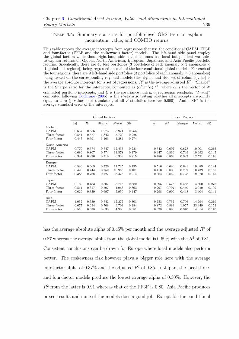
Chapter 6. Conditional Asset Pricing, Value, and Momentum in InternationalEquity Markets 239
Table 6.5: Summary statistics for portfolio-level GRS tests to explainmomentum, value, and COMBO returns
This table reports the average intercepts from regressions that use the conditional CAPM, FF3Fand four-factor (FF3F and the coskewness factor) models. The left-hand side panel employthe global factors while those right-hand side set of columns use local independent variablesto explain returns on Global, North American, European, Japanese, and Asia Pacific portfolioreturns. Specifically, there are 45 test portfolios (3 portfolios of each anomaly × 3 anomalies ×[1 global + 4 regions]) being regressed on each of the four conditional global models. For each ofthe four regions, there are 9 left-hand side portfolios (3 portfolios of each anomaly × 3 anomalies)being tested on the corresponding regional models (the right-hand side set of columns). |α| isthe average absolute intercept for a set of regressions. R2 is the average adjusted R2. “Sharpe”is the Sharpe ratio for the intercepts, computed as (α′Σ−1α)1/2; where α is the vector of N
estimated portfolio intercepts, and Σ is the covariance matrix of regression residuals. “F -stat”computed following Cochrane (2005), is the F -statistic testing whether all intercepts are jointlyequal to zero (p-values, not tabulated, of all F -statistics here are 0.000). And, “SE” is theaverage standard error of the intercepts.
Global Factors Local Factors
|α| R2 Sharpe F -stat SE |α| R2 Sharpe F -stat SEGlobalCAPM 0.637 0.556 1.273 5.974 0.255Three-factor 0.544 0.677 1.342 5.720 0.226Four-factor 0.445 0.691 1.463 4.284 0.274
North AmericaCAPM 0.779 0.674 0.747 12.435 0.221 0.642 0.697 0.678 10.001 0.215Three-factor 0.686 0.807 0.774 11.578 0.179 0.447 0.869 0.749 10.992 0.145Four-factor 0.384 0.820 0.719 6.339 0.215 0.486 0.869 0.982 12.591 0.176
EuropeCAPM 0.580 0.669 0.726 11.725 0.195 0.516 0.680 0.681 10.089 0.194Three-factor 0.426 0.744 0.752 10.953 0.181 0.410 0.808 0.739 10.739 0.155Four-factor 0.388 0.768 0.727 6.473 0.214 0.364 0.852 0.728 9.070 0.145
JapanCAPM 0.169 0.183 0.507 5.716 0.380 0.395 0.576 0.458 4.600 0.276Three-factor 0.514 0.327 0.507 4.963 0.363 0.297 0.797 0.450 3.929 0.199Four-factor 0.629 0.339 0.697 5.950 0.447 0.298 0.909 0.448 3.404 0.141
AsiaCAPM 1.052 0.539 0.742 12.272 0.303 0.753 0.757 0.796 14.294 0.219Three-factor 0.677 0.634 0.708 9.704 0.284 0.872 0.884 1.057 23.449 0.153Four-factor 0.516 0.638 0.633 4.906 0.351 0.628 0.896 0.970 14.014 0.170
has the average absolute alpha of 0.45% per month and the average adjusted R2 of
0.87 whereas the average alpha from the global model is 0.69% with the R2 of 0.81.
Consistent conclusions can be drawn for Europe where local models also perform
better. The coskewness risk however plays a bigger role here with the average
four-factor alpha of 0.37% and the adjusted R2 of 0.85. In Japan, the local three-
and four-factor models produce the lowest average alpha of 0.30%. However, the
R2 from the latter is 0.91 whereas that of the FF3F is 0.80. Asia Pacific produces
mixed results and none of the models does a good job. Except for the conditional

Chapter 6. Conditional Asset Pricing, Value, and Momentum in InternationalEquity Markets 240
CAPM, the average alphas from other local Asian models are lower than those of
the global factors. Local Asian models also have much higher explanatory power
with the R2 all higher than that of global counterparts.
In short, using portfolio returns as test assets, I can confirm the findings of Fama
and French (2012) that we should ask local models to explain local returns, suggest-
ing the fragmentation of international markets. Moreover, adding the coskewness
risk factor can enhance the explanatory power in most of the tests. The next sec-
tion will present my main findings using the new methodology from the previous
Chapter.
6.4 Time-varying risk adjustment at the compo-
nent level
I follow the methodology employed in the previous Chapter to adjust for the risk
of individual stocks in momentum and value portfolios. Specifically, I compute
time-varying risk-adjusted returns for each stock i in winner and loser portfolios
as follows.
radji,t = ri,t − rf −K∑j=1
(β>ijZt−1)f jt (6.9)
where radji,t is the risk-adjusted return for stock i that belongs to the winner or
loser portfolios at the end of each ranking period, t − 1. When the left-hand
side represents stock components in the global portfolios, f jt represents global
risk factors which are the excess global market return (Mkt), the global Fama
and French three factors (FF3F) and the coskewness risk factor SKS. Zt−1 is
the row vector of lagged instrumental variables, namely a constant, MSCI Global
DY, U.S. TERM and U.S. DEF. When the left-hand side represents returns in

Chapter 6. Conditional Asset Pricing, Value, and Momentum in InternationalEquity Markets 241
local portfolios, f jt can be either global risk factors or local risk factors in the
corresponding region. Then, Zt−1 is now the row vector of MSCI regional DY, U.S.
TERM and U.S. DEF. β>ij are the estimated constant loadings while Zt−1βi,t−1
are the conditional risk loadings on the factors.
As the last Chapter pointed out, betas from component-level regressions are biased
if we include ranking period returns in the estimation. By construction, winner
stocks are selected because of their increasing return while the loser stocks exhibit
the opposite trend during the ranking period. When these ranking period returns
are used as the left-hand side variable of regressions, the variable is no longer
randomly selected, causing the fundamental regression assumptions to be violated.
In particular, winner betas will be biased upwards while loser betas will be biased
downwards during bull markets, and vice versa for bear markets.
To avoid the bias, I follow the previous Chapter and exclude ranking period returns
from the estimation. Specifically, I estimate betas in the Equation (6.9) using
extending windows of returns on each stock i, starting from the first month to the
month prior to the ranking period. I use extending windows rather than fixed 120-
month windows as in the previous Chapter because my sample period is short with
only 222 months. Extending windows therefore give me more data and in turn
improve the accuracy of regressions. Fama and French (1992), Ferson and Harvey
(1999), Lettau and Ludvigson (2001), and Liu and Zhang (2008) also endorse the
use of extending windows.
The monthly risk-adjusted return for each stock (component) of the portfolio,
radji,t , will be the predicted return for stock i in month t + K where t is the first
month of holding period and K is the length of holding periods (i.e., skipping the
ranking period before we start holding the portfolio).13 To maintain meaningful
13The holding period for momentum portfolios is one month while that of value portfolios is12 months.

Chapter 6. Conditional Asset Pricing, Value, and Momentum in InternationalEquity Markets 242
regressions, I require stocks to have at least 24 valid monthly returns. The risk-
adjusted return on the portfolio will then be the average radji,t of all constituents in
the winner (high) portfolio minus the average of radji,t across loser (low) portfolios.
In other words, this method, which I also call component-level risk adjustment, is
simply replacing the observed return in the holding period by its predicted return
radji,t for each stock. The process of computing portfolio returns then proceeds
normally just as we form the raw portfolio.
Standard errors are computed following Cochrane (2005). Assuming that the
errors are i.i.d., the variance of estimated alphas can be computed by the following
formula:
var(α) =1
T(1 + µ>f Ω−1
f µf )Σ (6.10)
where µf is K × 1 mean vector of the risk factors; Ωf is the variance-covariance
matrix of the risk factors and Σ is the residual covariance matrix.14
Chordia and Shivakumar (2002) are among the first to use a set of macroeconomic
variables to adjust returns on individual winner and loser stocks. In other words,
their method is similar to the above, except that they do not have risk factors in
the model and also do not account for the biases caused by including the ranking
period in the estimation window. They find that momentum payoffs are strongly
related to business cycles as dated by the NBER, and consequently suggest that
momentum effects can potentially be explained by time-varying expected returns.
However, to be explained by rational theories, momentum payoffs must covary
with risk factors. As acknowledged by Chordia and Shivakumar (2002), the lack of
common risk factors in their model constrains their claims to only the correlation
between the predictive power of those variables and momentum payoffs. Moti-
vated by this limitation, Chapter 5 builds on Chordia and Shivakumar’s (2002)
14If the alpha is estimated using conditional models, f will include the risk factors and theirinteractions with the state variables.

Chapter 6. Conditional Asset Pricing, Value, and Momentum in InternationalEquity Markets 243
method to incorporate the common risk factors that have been empirically proved
to explain the cross section of returns. I also use a set of conditional asset pricing
models to tackle the time-varying betas of individual stocks. I find that applying
conditional FF3F models at component levels reduce the average momentum al-
pha by 50% in the U.S. markets. More importantly, Chapter 5 points out a bias
in the existing methodology, and after it is corrected, Chordia and Shivakumar’s
(2002) results are overturned.15
Given that conditional models perform nicely in the U.S., it is a convention to
investigate whether the explanatory power of those models and the component-
level risk adjustment methodology are robust in international data. Using the
new methodology, I also contribute to the international asset pricing literature
a new test of whether international markets are integrated. These questions are
examined in the rest of this Chapter.
In the next subsection, I employ global explanatory variables to explain returns
on both global and local versions of momentum, value, and COMBO portfolios. I
then repeat the exercise to use regional risk factors to explain regional portfolio
returns. The comparison of risk-adjusted returns from the two models will reveal
which model is better at pricing global and local anomalies (i.e., the average risk-
adjusted return should be lower)
15Wang and Wu (2011) also employ the unconditional FF3F model to adjust for the riskof individual stock components. The previous Chapter shows that this unconditional modeldoes not perform as well as conditional models. Results of Wang and Wu (2011) also sufferfrom ‘sample selection bias’ in which they include ranking period returns in running regressions.Chapter 5 shows that after correcting for the bias, the average risk-adjusted return from theunconditional FF3F model used in Wang and Wu (2011) increases by 20%.

Chapter 6. Conditional Asset Pricing, Value, and Momentum in InternationalEquity Markets 244
6.4.1 Time-varying risk adjustment using global risk fac-
tors
In this subsection, I employ global risk factors to subsequently explain returns on
momentum, value, and COMBO portfolios. I also focus on investigating whether
the global conditional model, being applied on individual components’ returns,
can reduce the portfolio-level alpha reported in Subsection 6.3.4. In the next
subsection, I will compare the explanatory power of these global models with that
of local models.
Risk-adjusted momentum returns
Table 6.6 reports average component-level risk-adjusted returns on momentum
portfolios where the explanatory variables are global risk factors. In panel A, I
regress individual stock (component) returns in the global momentum portfolio
on global explanatory variables and their interactions with the set of global in-
strumental variables. The global conditional CAPM fares poorly in rationalizing
global momentum returns with the average alpha of 0.86% per month (t=3.25) – a
reduction of only 3bps from the raw average return in Table 6.2, but it is a decrease
of 25bps from the portfolio-level estimate in the first column (first Panel) of Table
6.4. The global conditional FF3F model performs better by reducing the average
momentum alpha to 0.68% with an associated t-statistic of 2.48, statistically sig-
nificant at the 5% level. It is also a 42% reduction in alpha over the portfolio-level
estimate. Thus, consistent the previous Chapter’s findings, the conditional FF3F
model, being applied at the component level, can correctly predict the behavior of
winner and loser stocks. The best performer is the conditional four-factor model,
which contains FF3F and coskewness factor, although the improvement over the
FF3F model’s alpha is only 6bps.

Chapter 6. Conditional Asset Pricing, Value, and Momentum in InternationalEquity Markets 245
Panel B uses global risk factors to explain returns on North American momentum
portfolios. Surprisingly, the global conditional CAPM performs just as well as
the conditional FF3F model. The average momentum alpha from the conditional
global CAPM is 0.56% per month (t=2.24), compared with the FF3F’s alpha
of 0.53% (t=2.00, statistically significant at the 5% level). These represent 42%
and 51% reductions over the corresponding portfolio-level estimates in Table 6.4.
Adding the coskewness factor however increases the average alpha to 0.72% per
month (t=2.73, statistically significant at the 1% level), suggesting that this factor
does not help explain momentum returns in North America. Thus, the global
conditional CAPM and FF3F should be used to rationalize momentum returns in
North American markets.
Panel C reports average risk-adjusted momentum returns for Europe. The con-
ditional global CAPM yields the average winner-minus-loser alpha of 1.17% per
month (t=4.33), which is 19% lower than the portfolio-level alpha in Table 6.4.
The conditional global FF3F model fares slightly better by further reducing the
average alpha to 1.08% (t=4.78), still large and statistically significant at the 1%
level although the reduction of 30% from the portfolio-level alpha is economically
significant. The global four-factor model does not help much in rationalizing mo-
mentum returns with the average alpha of 1.06% per month (t=4.71). Although
the evidence suggests that the conditional global four-factor model should be used
to explain momentum returns in European markets, the improvement from this
model is not economically large to make it more appealing than the conditional
global FF3F model.
Turning to risk-adjusted momentum returns in Japan and Asia Pacific; all global
models perform well in Japan, which is not surprising because momentum strate-
gies are not profitable there. Asia Pacific is a region where the global factors do
not work well. The global four-factor model is again the worst performer, with
the average risk-adjusted return of 1.34% per month, which is much higher than

Chapter 6. Conditional Asset Pricing, Value, and Momentum in InternationalEquity Markets 246
Table 6.6: Risk-adjusted momentum returns using global risk factors,July 1993 to Dec 2011
This table reports average component-level risk-adjusted returns on momentum portfolios in fourregions and the global market. I run extending-window regressions of returns of individual stocks(components) on the global risk factors. The “three-factor” model of Fama and French (1993)(FF3F) consists of the market risk, SMB, and HML factors downloaded from Ken French’s web-site. The “four-factor” model consists of the FF3F and Harvey and Siddique (2000) coskewnessfactor. Global models’ conditioning information includes a constant, MSCI World dividend yield(DIV), U.S. lagged term spread (TERM) and U.S. lagged default spread (DEF). I use extending-window of component returns to estimate Equation (6.9) starting from the first month to themonth prior to the ranking period, with 24 valid returns required (this requirement was im-posed when constructing the portfolio). Standard errors are adjusted using Formula (6.10) andt-statistics are reported in parentheses. ∗, ∗∗, ∗ ∗ ∗ represent the significance levels at 10%, 5%and 1%, respectively.
Models High Low HML Sharpe
Panel A: Global PortfoliosCAPM 0.85 −0.01 0.86 0.76
(4.63)∗∗∗ (−0.04) (3.25)∗∗∗
FF3F 0.56 −0.12 0.68 0.58(3.77)∗∗∗ (−0.49) (2.48)∗∗
Four-factor 0.19 −0.44 0.62 0.52(1.22) (−1.79)∗ (2.24)∗∗
Panel B: North AmericaCAPM 0.86 0.30 0.56 0.48
(3.63)∗∗∗ (0.90) (2.24)∗∗
FF3F 0.66 0.13 0.53 0.46(2.59)∗∗∗ (0.38) (2.00)∗∗
Four-factor 0.47 −0.25 0.72 0.63(2.19)∗∗ (−0.77) (2.73)∗∗∗
Panel C: EuropeCAPM 0.92 −0.25 1.17 1.32
(4.40)∗∗∗ (−0.97) (5.69)∗∗∗
FF3F 0.66 −0.42 1.08 1.11(2.62)∗∗∗ (−1.48) (4.78)∗∗∗
Four-factor 0.14 −0.92 1.06 1.10(0.52) (−3.30)∗∗∗ (4.71)∗∗∗
Panel D: JapanCAPM −0.22 −0.20 −0.02 −0.02
(−0.58) (−0.42) (−0.07)FF3F −0.19 −0.07 −0.12 −0.10
(−0.38) (−0.11) (−0.42)Four-factor −0.48 −0.53 0.05 0.04
(−0.96) (−0.86) (0.15)
Panel E: Asia (Ex. Japan)CAPM 1.41 0.31 1.10 0.84
(4.52)∗∗∗ (0.79) (3.61)∗∗∗
FF3F 0.99 −0.15 1.14 0.84(3.14)∗∗∗ (−0.41) (3.60)∗∗∗
Four-factor 0.65 −0.68 1.34 0.90(1.82)∗ (−1.58) (3.86)∗∗∗
the raw average profit of 1.14% per month. The best performing model is the
global CAPM, which produces the average alpha of 1.10% (t=3.61, statistically
significant at the 1% level) and is 31% lower than the corresponding portfolio al-
pha. The global conditional FF3F model does not offer any improvement with the

Chapter 6. Conditional Asset Pricing, Value, and Momentum in InternationalEquity Markets 247
averge alpha of 1.14% per month (t=3.60) although it is still 52bps lower than the
portfolio alpha. Consequently, the parsimonious global conditional CAPM should
be used to explain Asian momentum returns
In short, consistent with the findings of Chapter 5, component-level risk adjust-
ment can help improve the explanatory power of conditional asset pricing models
by reducing the average momentum alpha in all regions although the effect remains
strong. The failure of global asset pricing models may be the result of market isola-
tion (or simply bad model problem), which will be explored in the next subsection.
The most important conclusion is that, in contrast to the portfolio-level evidence
whose momentum alphas are all higher than raw returns, the component-level risk
adjustment offers improvement in all markets.
Risk-adjusted value returns
We now turn to Table 6.7 in which the left-hand side of Equation (6.9) is the return
on value portfolios. Similar to the previous Table, I regress returns on individual
components of the value portfolio on global risk factors and their interactions with
conditioning variables. Panel A reports the average high-minus-low (HML) alpha
of global value portfolios. The conditional global CAPM is the worst performer
with the average alpha of 0.90% per month (t= 5.17), which is even 5bps higher
than the raw average profit and therefore offers no improvement over the portfolio-
level estimate in the second column of Table 6.7. The best model is the global FF3F
in which the average value alpha is reduced to only 0.49% per month (t=2.92) – a
9bps reduction compared with the portfolio-level measure. The four-factor model
fares worse than the conditional FF3F model with the average alpha of 0.65% per
month (t=3.68). Consequently, the conditional global FF3F should be used to
explain global value returns.

Chapter 6. Conditional Asset Pricing, Value, and Momentum in InternationalEquity Markets 248
In North America, the global conditional FF3F model is also the best model,
yielding the average HML alpha of 0.28% per month (t= 1.56), which is statistically
insignificant even at the 10% level. This compares favorably with the portfolio-
level value alpha of 0.58% per month in Table 6.7. The conditional four-factor
model yields the average alpha of 0.61% per month (t=3.18), which is still higher
than that of the FF3F model. The conditional CAPM is the worst model, with the
average risk-adjusted return of 0.88% per month (t=4.52), which is 4bps higher
than the raw average profit. Therefore, we should use the global conditional FF3F
model to explain value returns in North America.
In Europe, the best model is the global four-factor (FF3F and the coskewness
factor) model, producing the average alpha of only 0.25% per month (t=1.42),
which is approximately 55% or 32% reduction from the raw profit and four-
factor portfolio-level alpha respectively. The worst model is the global conditional
CAPM and the second best model is the global FF3F model, having the average
risk-adjusted returns of 0.50% (t=3.27) and 0.40% (t=2.53), respectively. Thus,
coskewness plays a more important role in Europe than in other regions and we
should use the global conditional four-factor to explain value returns in European
markets.
The global CAPM is again the worst performer in Asia and Japan. The best
performing model in Japan is the global conditional FF3F model with the average
alpha of 0.46% per month and an associated t-statistic of 2.16 – statistically signifi-
cant at the 5% level. This average alpha is a 12bps decrease from the portfolio-level
alpha. In Asia, the global conditional four-factor performs the best, earning the
average risk-adjusted return of 0.94% per month (t=3.30), which is a 39% reduc-
tion from the raw return. However, this average alpha is still a failure compared
with the portfolio-level risk adjustment in Table 6.7, which is 14bps lower. Con-
sequently, we would not apply global models at the component level to explain
value returns in Asia because the portfolio-level risk adjustment performs better.

Chapter 6. Conditional Asset Pricing, Value, and Momentum in InternationalEquity Markets 249
Table 6.7: Risk-adjusted value returns using global risk factors, July 1993to Dec 2011
This table reports average component-level risk-adjusted returns on value portfolios in 4 re-gions and the global market. I run extending-window regressions of returns of individual stocks(components) on the global risk factors. The “three-factor” model of Fama and French (1993)(FF3F) consists of the market risk, SMB, and HML factors downloaded from Ken French’s web-site. The “four-factor” model consists of the FF3F and Harvey and Siddique (2000) coskewnessfactor. Global models’ conditioning information includes a constant, MSCI World dividend yield(DIV), U.S. lagged term spread (TERM) and U.S. lagged default spread (DEF). I use extending-window of component returns to estimate Equation (6.9) starting from the first month to themonth prior to the ranking period, with 24 valid returns required (this requirement was im-posed when constructing the portfolio). Standard errors are adjusted using Formula (6.10) andt-statistics are reported in parentheses. ∗, ∗∗, ∗ ∗ ∗ represent the significance levels at 10%, 5%and 1%, respectively.
Models High Low HML Sharpe
Panel A: Global PortfoliosCAPM 1.06 0.16 0.90 1.20
(4.79)∗∗∗ (0.94) (5.17)∗∗∗
FF3F 0.62 0.13 0.49 0.68(3.61)∗∗∗ (0.92) (2.92)∗∗∗
Four-factor 0.46 −0.19 0.65 0.86(2.28)∗∗ (−1.24) (3.68)∗∗∗
Panel B: North AmericaCAPM 1.21 0.32 0.88 1.05
(4.29)∗∗∗ (1.34) (4.52)∗∗∗
FF3F 0.64 0.35 0.28 0.36(2.25)∗∗ (1.31) (1.56)
Four-factor 0.56 −0.05 0.61 0.74(1.54) (−0.18) (3.18)∗∗∗
Panel C: EuropeCAPM 0.71 0.22 0.50 0.76
(3.49)∗∗∗ (1.00) (3.27)∗∗∗
FF3F 0.62 0.22 0.40 0.59(2.52)∗∗ (0.80) (2.53)∗∗
Four-factor 0.05 −0.20 0.25 0.33(0.18) (−0.75) (1.42)
Panel D: JapanCAPM 0.36 −0.48 0.84 1.01
(0.79) (−1.23) (4.35)∗∗∗
FF3F −0.20 −0.66 0.46 0.50(−0.34) (−1.26) (2.16)∗∗
Four-factor −0.21 −0.70 0.50 0.51(−0.31) (−1.13) (2.20)∗∗
Panel E: Asia (Ex. Japan)CAPM 1.62 0.09 1.53 1.64
(4.61)∗∗∗ (0.30) (7.06)∗∗∗
FF3F 1.19 0.18 1.01 1.00(3.52)∗∗∗ (0.61) (4.30)∗∗∗
Four-factor 0.77 −0.17 0.94 0.77(1.74)∗ (−0.39) (3.30)∗∗∗
Risk-adjusted 50-50 COMBO returns
AMP find that a 50-50 COMBO portfolio that equally combines value and mo-
mentum strategies earns a stable and large return in all regions and the global
Chapter 6. Conditional Asset Pricing, Value, and Momentum in InternationalEquity Markets 250
market. I now examine whether COMBO portfolios are still strong after adjusting
for the risk of individual stocks (components) using global explanatory variables.
Table 6.8 shows average risk-adjusted returns on COMBO portfolios, which are the
equal-weighted average of the two portfolio returns from the previous two tables.
Panel A shows that the global conditional CAPM still cannot rationalize the global
COMBO anomaly. The average HMLCOMBO alpha of global portfolios remains
almost equal to the raw average profit at 0.88% per month with the significant
associated t-statistic of 6.78. The correlation between value and momentum is
−0.45, which is even more negative than the raw correlation in the panel C of Table
6.2, causing the risk-adjusted COMBO portfolio to be persistent. The annualized
Sharpe ratio after risk adjustment is 1.58, which is higher than the Sharpe ratios
of stand-alone momentum (0.76) and value portfolios (1.20). This average alpha
is still lower than the 1.01% per month of the portfolio-level estimate (the third
column of Table 6.8).
The global conditional FF3F model is the best, which has the average risk-adjusted
COMBO return of 0.59% per month, but the t-statistic of 4.14 is still statisti-
cally significant at the 1% level. This is approximately a 33% reduction over the
component-level CAPM estimate and the portfolio-level alpha in Table 6.4. The
Sharpe ratio also decreases to 0.96, which is still higher than 0.58 of momentum
portfolios and 0.68 of value portfolios. The conditional four-factor model, which
adds the coskewness risk factor to the baseline FF3F model, increases the aver-
age alpha to 0.64% per month (t = 4.47). These findings, together with those of
momentum and value effects in the previous two tables, suggest that the global
conditional FF3F should be used to explain returns on global COMBO portfolios.
Panel B shows a similar picture in North America that the global conditional
FF3F model is the best among the three competing models. The average risk-
adjusted return from the conditional FF3F model is 0.41% per month (t=3.73),
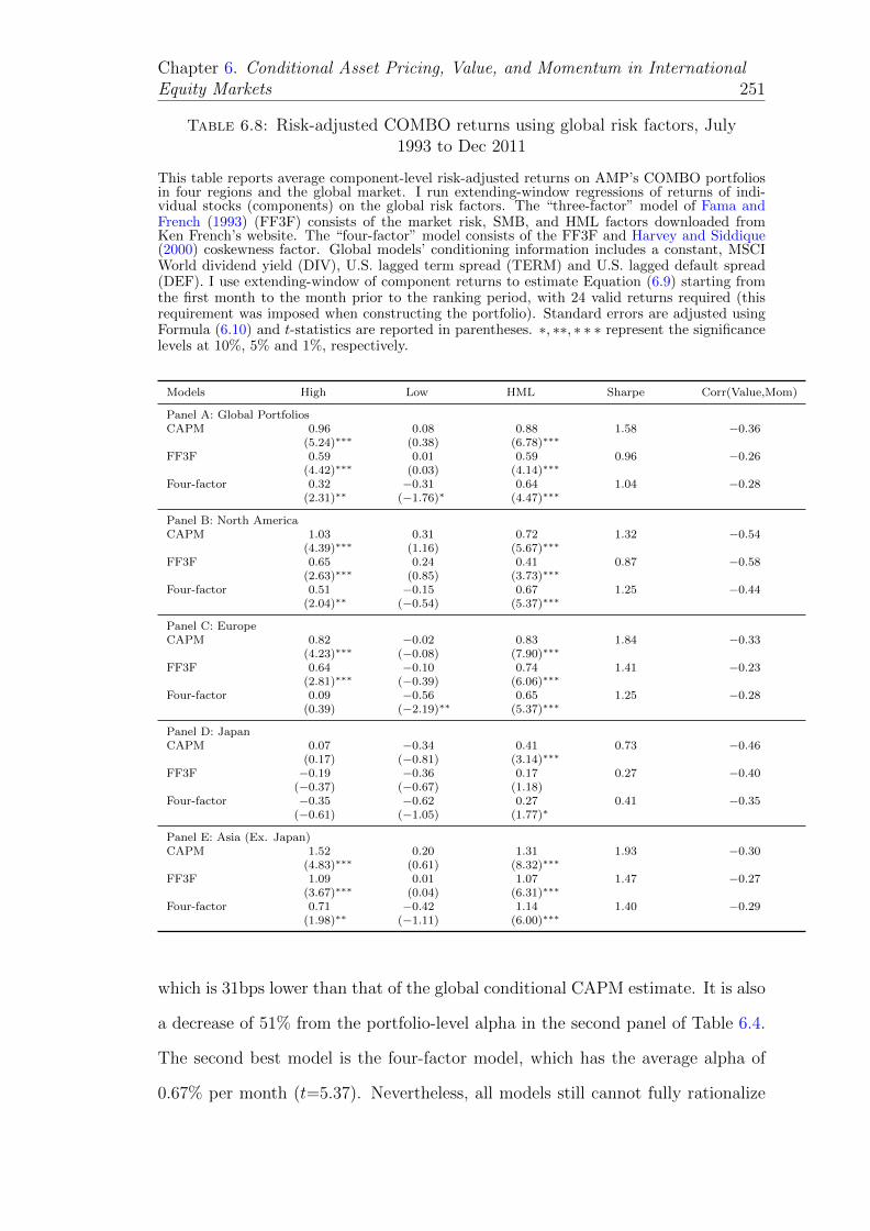
Chapter 6. Conditional Asset Pricing, Value, and Momentum in InternationalEquity Markets 251
Table 6.8: Risk-adjusted COMBO returns using global risk factors, July1993 to Dec 2011
This table reports average component-level risk-adjusted returns on AMP’s COMBO portfoliosin four regions and the global market. I run extending-window regressions of returns of indi-vidual stocks (components) on the global risk factors. The “three-factor” model of Fama andFrench (1993) (FF3F) consists of the market risk, SMB, and HML factors downloaded fromKen French’s website. The “four-factor” model consists of the FF3F and Harvey and Siddique(2000) coskewness factor. Global models’ conditioning information includes a constant, MSCIWorld dividend yield (DIV), U.S. lagged term spread (TERM) and U.S. lagged default spread(DEF). I use extending-window of component returns to estimate Equation (6.9) starting fromthe first month to the month prior to the ranking period, with 24 valid returns required (thisrequirement was imposed when constructing the portfolio). Standard errors are adjusted usingFormula (6.10) and t-statistics are reported in parentheses. ∗, ∗∗, ∗ ∗ ∗ represent the significancelevels at 10%, 5% and 1%, respectively.
Models High Low HML Sharpe Corr(Value,Mom)
Panel A: Global PortfoliosCAPM 0.96 0.08 0.88 1.58 −0.36
(5.24)∗∗∗ (0.38) (6.78)∗∗∗
FF3F 0.59 0.01 0.59 0.96 −0.26(4.42)∗∗∗ (0.03) (4.14)∗∗∗
Four-factor 0.32 −0.31 0.64 1.04 −0.28(2.31)∗∗ (−1.76)∗ (4.47)∗∗∗
Panel B: North AmericaCAPM 1.03 0.31 0.72 1.32 −0.54
(4.39)∗∗∗ (1.16) (5.67)∗∗∗
FF3F 0.65 0.24 0.41 0.87 −0.58(2.63)∗∗∗ (0.85) (3.73)∗∗∗
Four-factor 0.51 −0.15 0.67 1.25 −0.44(2.04)∗∗ (−0.54) (5.37)∗∗∗
Panel C: EuropeCAPM 0.82 −0.02 0.83 1.84 −0.33
(4.23)∗∗∗ (−0.08) (7.90)∗∗∗
FF3F 0.64 −0.10 0.74 1.41 −0.23(2.81)∗∗∗ (−0.39) (6.06)∗∗∗
Four-factor 0.09 −0.56 0.65 1.25 −0.28(0.39) (−2.19)∗∗ (5.37)∗∗∗
Panel D: JapanCAPM 0.07 −0.34 0.41 0.73 −0.46
(0.17) (−0.81) (3.14)∗∗∗
FF3F −0.19 −0.36 0.17 0.27 −0.40(−0.37) (−0.67) (1.18)
Four-factor −0.35 −0.62 0.27 0.41 −0.35(−0.61) (−1.05) (1.77)∗
Panel E: Asia (Ex. Japan)CAPM 1.52 0.20 1.31 1.93 −0.30
(4.83)∗∗∗ (0.61) (8.32)∗∗∗
FF3F 1.09 0.01 1.07 1.47 −0.27(3.67)∗∗∗ (0.04) (6.31)∗∗∗
Four-factor 0.71 −0.42 1.14 1.40 −0.29(1.98)∗∗ (−1.11) (6.00)∗∗∗
which is 31bps lower than that of the global conditional CAPM estimate. It is also
a decrease of 51% from the portfolio-level alpha in the second panel of Table 6.4.
The second best model is the four-factor model, which has the average alpha of
0.67% per month (t=5.37). Nevertheless, all models still cannot fully rationalize

Chapter 6. Conditional Asset Pricing, Value, and Momentum in InternationalEquity Markets 252
COMBO returns even though they are quite successful in explaining individual
stand-alone anomalies. The Sharpe ratio from the FF3F model is 0.87, which is
much higher than 0.46 of momentum strategies and 0.36 of value portfolios.
Panel C reports average risk-adjusted HMLCOMBO returns in Europe. Again,
none of the models can explain the COMBO profit. The worst model is still the
conditional CAPM, which has the average alpha of 0.83% per month (t=7.90) and
the associated annualized Sharpe ratio of 1.84 which is even higher than that of the
raw COMBO return (1.55). The conditional FF3F model reduces the average risk-
adjusted return to 0.74% per month (t=6.06) and the Sharpe ratio is 1.41. The
best model is the global conditional four-factor model, which has the average alpha
of 0.67% per month (t=5.37) and the Sharpe ratio of 1.25. Thus, the coskewness
risk is again more important in Europe.
Panel E presents average risk-adjusted COMBO returns for Asia. The best per-
former is the global conditional FF3F model and the worst model is the global
conditional CAPM. The average risk-adjusted return from the conditional CAPM
is 1.31% per month (t=8.32) and the associated Sharpe ratio is 1.93, which is
higher than that of the raw COMBO portfolio (1.81). The global conditional
FF3F model can reduce the average COMBO alpha to 1.07% (t=6.31), which is
much less than the portfolio-level alpha of 1.43%. Adding the coskewness risk
does not improve the performance of the FF3F model as the average risk-adjusted
return increases to 1.14% per month although the Sharpe ratio is reduced to 1.40.
Therefore, the global conditional FF3F model is still the best performer in Asia.
Panel D shows average alphas for COMBO portfolios in Japan. In contrast to
other regions, COMBO returns in Japan can be explained by the global conditional
FF3F model with the Sharpe ratio of 0.27, the average alpha being equal to 0.17%
per month – statistically insignificant even at the 10% level. This success of FF3F
model is somewhat not surprising because the previous section has shown that the
Chapter 6. Conditional Asset Pricing, Value, and Momentum in InternationalEquity Markets 253
COMBO anomaly is weak in Japan. The global conditional CAPM still cannot
explain the COMBO anomaly in Japan with the Sharpe ratio of 0.73, which is
higher than the raw COMBO portfolio’s Sharpe of 0.69.
In short, except for Japan, we confirm AMP’s findings that COMBO returns are
strong and persistent everywhere. The global conditional FF3F model, being ap-
plied on individual stocks, is the best out of three competing models everywhere
but Europe where the four-factor model performs best. Also, adding the coskew-
ness risk does not offer improvement over the FF3F model in any region but
Europe.
6.4.2 Time-varying risk adjustment using local risk factors
In this subsection, I investigate whether local risk factors have higher explanatory
power than the global counterparts in explaining local portfolio returns. I repeat
the exercise in the previous subsection with the right-hand side of the regression
being the corresponding local risk factors and their interaction terms with con-
ditioning variables for each region. The main analysis focuses on comparing the
average alpha from local regressions with that from global tests in the previous
subsection. The main conclusion is that, based on the magnitude of reduction
in average risk-adjusted returns, international markets are integrated everywhere
except in Europe. Except for Europe where we should use local risk factors to
explain local stock returns, global risk factors produce lower average pricing errors
in North America, Japan, and Asia.
Risk-adjusted momentum returns
Panel A of Table 6.9 reports the average risk-adjusted return on North American
momentum portfolios using three alternative local North American asset pricing

Chapter 6. Conditional Asset Pricing, Value, and Momentum in InternationalEquity Markets 254
models. Comparing local average alphas with global average alphas in Table 6.6, all
local models have higher risk-adjusted returns than their global counterparts. The
local conditional CAPM has the average alpha of 0.70% per month (t=2.35), which
is 14bps higher than that of the global CAPM. Similar to the global evidence, the
local conditional FF3F is the best model out of three competing specifications, but
its average alpha is still 13bps higher than that of the global FF3F estimate. The
local four-factor model is the worst performer, producing the average risk-adjusted
return of 0.79% per month (t=2.72).
Panel B reports average local momentum alphas in Europe. In contrast to the
North American evidence, local models perform better than the global factors.
The local conditional three-factor model has the average alpha of 0.83% per month
(t=4.09), which is 23% lower than the corresponding global estimate. Similar to
the global evidence, the conditional four-factor model, which adds the coskew-
ness risk, fares best with the average risk-adjusted return of 0.76% per month
(t=3.62), which is approximately 28% lower than the global four-factor estimate.
Consequently, we should use local four-factor model to explain portfolio returns
in Europe. This support for local models in Europe is consistent with Fama and
French (2012) even though my methodology is different.
Panel C and D show the statistics for Japan and Asia Pacific. It is not unexpected
that local models do well in Japan since the momentum effect is not present
there. In Asia, we can see that the best performer is the conditional three-factor
model, but it still has a higher average pricing error than its global version. The
average WML alpha from the local three-factor model is 1.31% (t=3.86), which is
almost 17bps higher than the corresponding global alpha. The four-factor model
is the worst performer in Asia, yielding the average alpha of 1.84% per month
(t=3.61), which 50bps higher than the global four-factor estimate. These average
risk-adjusted returns are all much higher than the corresponding global estimates
in Table 6.6.

Chapter 6. Conditional Asset Pricing, Value, and Momentum in InternationalEquity Markets 255
Table 6.9: Risk-adjusted momentum returns using local risk factors, July1993 to Dec 2011
This table reports average component-level risk-adjusted returns on momentum portfolios in fourregions. I run extending-window regressions of returns of individual stocks (components) on thelocal risk factors. The “three-factor” model of Fama and French (1993) (FF3F) consists of themarket risk, SMB, and HML factors downloaded from Ken French’s website. The “four-factor”model consists of the FF3F and Harvey and Siddique (2000) coskewness factor. Local models’conditioning information includes a constant, the local MSCI DIV, U.S. TERM and U.S. DEF.I use extending-window of component returns to estimate Equation (6.9) starting from the firstmonth to the month prior to the ranking period, with 24 valid returns required (this requirementwas imposed when constructing the portfolio). Standard errors are adjusted using Formula (6.10)and t-statistics are reported in parentheses. ∗, ∗∗, ∗ ∗ ∗ represent the significance levels at 10%,5% and 1%, respectively.
Models High Low HML Sharpe
Panel A: North AmericaCAPM 0.45 −0.25 0.70 0.55
(1.95)∗ (−0.76) (2.35)∗∗
FF3F 0.26 −0.40 0.66 0.55(1.67)∗ (−1.42) (2.36)∗∗
Four-factor 0.05 −0.73 0.79 0.63(0.29) (−2.52)∗∗ (2.72)∗∗∗
Panel B: EuropeCAPM 0.74 −0.40 1.14 1.32
(3.68)∗∗∗ (−1.58) (5.69)∗∗∗
FF3F 0.58 −0.24 0.83 0.95(3.18)∗∗∗ (−1.00) (4.09)∗∗∗
Four-factor 0.32 −0.43 0.76 0.84(1.77)∗ (−1.95)∗ (3.62)∗∗∗
Panel C: JapanCAPM 0.07 −0.01 0.08 0.07
(0.25) (−0.04) (0.29)FF3F 0.06 0.05 0.01 0.01
(0.29) (0.18) (0.05)Four-factor −0.25 −0.24 −0.01 −0.01
(−1.24) (−0.82) (−0.02)
Panel D: Asia (Ex. Japan)CAPM 1.39 0.02 1.37 0.79
(3.31)∗∗∗ (0.05) (3.41)∗∗∗
FF3F 1.40 0.09 1.31 0.90(4.13)∗∗∗ (0.24) (3.86)∗∗∗
Four-factor 1.57 −0.27 1.84 0.84(2.30)∗∗ (−0.56) (3.61)∗∗∗
In short, by comparing Tables 6.6 and 6.9 for momentum portfolios, we should
use the global conditional FF3F model to explain momentum returns in North
America, Japan, and Asia Pacific while the local conditional four-factor model
should be used in Europe.
Chapter 6. Conditional Asset Pricing, Value, and Momentum in InternationalEquity Markets 256
Risk-adjusted value returns
Table 6.10 reports average risk-adjusted returns on value strategies in which I
regress returns on individual stocks within the value portfolio on local factors and
their interactions with the set of local conditioning information. Compared with
the performance global models, local risk factors are considered failure in North
America in explaining the value effect. The worst performer is the conditional
four-factor model, which produces the average HML risk-adjusted return of 1.32%
per month – more than doubled the corresponding global estimate of 0.61% per
month. The local conditional FF3F fares best, but its average alpha is 0.65% per
month (t=2.69), which is 37bps higher than that of the global FF3F estimate.
Thus, global models outperform all of their local North American counterparts in
explaining the value anomaly.
Similar to the above evidence for momentum effects, local conditional models do
a better job in explaining value returns in Europe. The best performing model is
again the local conditional four-factor model with the average alpha of 19bps per
month (t–statistic=0.97 – statistically insignificant even at the 10% level).
Among the local models in Japan, the four-factor model also fares best with the
average alpha of 0.60% per month (t=3.56), which is 25bps and 9bps lower than
those of CAPM and FF3F models, respectively. However, this average alpha is
still 14bps higher than that of the global FF3F model (0.46% per month from
Table 6.7). Consequently, we should use the global three-factor model to explain
value returns in Japanese markets.
The last panel of Table 6.10 shows average value alphas in Asia. Although the
evidence of market integration is mixed since different models produce different
conclusions, the local conditional FF3F has the lowest average alpha among all
models. The local conditional FF3F produces the lowest alpha of 0.88% per month

Chapter 6. Conditional Asset Pricing, Value, and Momentum in InternationalEquity Markets 257
Table 6.10: Risk-adjusted value returns using local risk factors, July 1993to Dec 2011
This table reports average component-level risk-adjusted returns on value portfolios in fourregions. I run extending-window regressions of returns of individual stocks (components) on thelocal risk factors. The “three-factor” model of Fama and French (1993) (FF3F) consists of themarket risk, SMB, and HML factors downloaded from Ken French’s website. The “four-factor”model consists of the FF3F and Harvey and Siddique (2000) coskewness factor. Local models’conditioning information includes a constant, the local MSCI DIV, U.S. TERM and U.S. DEF.I use extending-window of component returns to estimate Equation (6.9) starting from the firstmonth to the month prior to the ranking period, with 24 valid returns required (this requirementwas imposed when constructing the portfolio). Standard errors are adjusted using Formula (6.10)and t-statistics are reported in parentheses. ∗, ∗∗, ∗ ∗ ∗ represent the significance levels at 10%,5% and 1%, respectively.
Models High Low HML Sharpe
Panel A: North AmericaCAPM 0.93 −0.24 1.17 1.31
(3.39)∗∗∗ (−1.02) (5.63)∗∗∗
FF3F 0.45 −0.19 0.65 0.62(1.64) (−1.09) (2.69)∗∗∗
Four-factor 0.51 −0.82 1.32 1.17(1.72)∗ (−4.30)∗∗∗ (5.05)∗∗∗
Panel B: EuropeCAPM 0.65 0.11 0.54 0.84
(3.13)∗∗∗ (0.51) (3.63)∗∗∗
FF3F 0.37 0.13 0.24 0.34(1.93)∗ (0.61) (1.44)
Four-factor −0.37 −0.56 0.19 0.23(−0.98) (−1.40) (0.97)
Panel C: JapanCAPM 0.58 −0.28 0.85 1.02
(1.76)∗ (−1.01) (4.41)∗∗∗
FF3F 0.44 −0.25 0.69 1.00(1.83)∗ (−1.06) (4.29)∗∗∗
Four-factor 0.25 −0.34 0.60 0.83(0.94) (−1.34) (3.56)∗∗∗
Panel D: Asia (Ex. Japan)CAPM 0.98 −0.48 1.46 1.39
(2.73)∗∗∗ (−1.39) (5.99)∗∗∗
FF3F 0.24 −0.63 0.88 0.44(0.30) (−1.28) (1.89)∗
Four-factor 1.31 −1.06 2.37 0.89(3.79)∗∗∗ (−1.76)∗ (3.82)∗∗∗
(t=1.89, statistically significant at the 10% level), which is lower than the corre-
sponding estimate from the global FF3F model (1.01% per month) – suggesting
that local conditional FF3F model should be used to explain value returns in Asia.
In short, by comparing Tables 6.7 and 6.10 for value portfolios, we should only
use the global conditional FF3F model to explain value returns in North America
and Japan. The local four-factor (FF3F and coskewness factor) model should be
employed in Europe and the local FF3F model should be used to explain value
Chapter 6. Conditional Asset Pricing, Value, and Momentum in InternationalEquity Markets 258
returns in Asia Pacific.
Risk-adjusted 50-50 COMBO returns
Table 6.11 shows average HMLCOMBO alphas from local conditional models. Sim-
ilar to the previous subsection, local models perform worse than their global coun-
terparts in North America. The local conditional FF3F model gives the lowest
average alpha of 0.65% (t=4.65), but it is still higher than the 0.41% average al-
pha of the global conditional FF3F model (Table 6.8). Consequently, we should
use the global conditional FF3F model to explain returns in North America.
Consistent with the previous findings, the local conditional four-factor model is
again the best performer in Europe, producing the average alpha of 0.47% per
month (t=3.68), which is lower than 0.65% per month of the global estimate
(Table 6.8). Thus, we should use local four-factor (FF3F and the coskewness
factor) model to explain returns in European markets.
The evidence in Japan and Asia is contrary to that in Europe. Average risk-
adjusted returns on COMBO portfolios remain large and statistically significant
for all models. In Japan, the local four-factor model is the best among local
models with the average alpha of 0.30% per month (t=2.39), but it is still higher
than 0.17% per month (t=1.18) of its global FF3F counterpart. Therefore, we
should employ the global FF3F model to explain returns in Japan rather than
local models.
Similar (though weaker) result is also found in Asia where global risk factors tend
to have higher explanatory power. Among local models, the conditional FF3F
model is the best with the lowest average alpha of 1.10% per month (t=6.31),
which is, nevertheless, still slightly higher than the 1.07% per month from the
global version. Of notice is the significant failure of the local four-factor model.
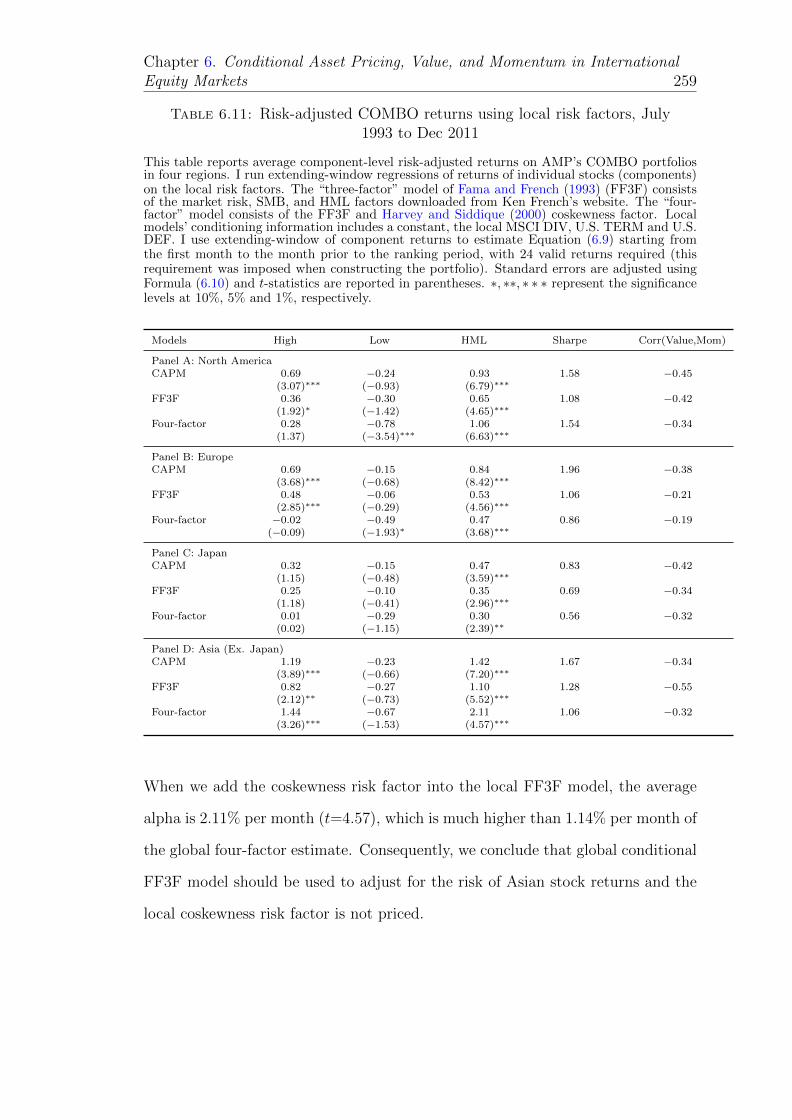
Chapter 6. Conditional Asset Pricing, Value, and Momentum in InternationalEquity Markets 259
Table 6.11: Risk-adjusted COMBO returns using local risk factors, July1993 to Dec 2011
This table reports average component-level risk-adjusted returns on AMP’s COMBO portfoliosin four regions. I run extending-window regressions of returns of individual stocks (components)on the local risk factors. The “three-factor” model of Fama and French (1993) (FF3F) consistsof the market risk, SMB, and HML factors downloaded from Ken French’s website. The “four-factor” model consists of the FF3F and Harvey and Siddique (2000) coskewness factor. Localmodels’ conditioning information includes a constant, the local MSCI DIV, U.S. TERM and U.S.DEF. I use extending-window of component returns to estimate Equation (6.9) starting fromthe first month to the month prior to the ranking period, with 24 valid returns required (thisrequirement was imposed when constructing the portfolio). Standard errors are adjusted usingFormula (6.10) and t-statistics are reported in parentheses. ∗, ∗∗, ∗ ∗ ∗ represent the significancelevels at 10%, 5% and 1%, respectively.
Models High Low HML Sharpe Corr(Value,Mom)
Panel A: North AmericaCAPM 0.69 −0.24 0.93 1.58 −0.45
(3.07)∗∗∗ (−0.93) (6.79)∗∗∗
FF3F 0.36 −0.30 0.65 1.08 −0.42(1.92)∗ (−1.42) (4.65)∗∗∗
Four-factor 0.28 −0.78 1.06 1.54 −0.34(1.37) (−3.54)∗∗∗ (6.63)∗∗∗
Panel B: EuropeCAPM 0.69 −0.15 0.84 1.96 −0.38
(3.68)∗∗∗ (−0.68) (8.42)∗∗∗
FF3F 0.48 −0.06 0.53 1.06 −0.21(2.85)∗∗∗ (−0.29) (4.56)∗∗∗
Four-factor −0.02 −0.49 0.47 0.86 −0.19(−0.09) (−1.93)∗ (3.68)∗∗∗
Panel C: JapanCAPM 0.32 −0.15 0.47 0.83 −0.42
(1.15) (−0.48) (3.59)∗∗∗
FF3F 0.25 −0.10 0.35 0.69 −0.34(1.18) (−0.41) (2.96)∗∗∗
Four-factor 0.01 −0.29 0.30 0.56 −0.32(0.02) (−1.15) (2.39)∗∗
Panel D: Asia (Ex. Japan)CAPM 1.19 −0.23 1.42 1.67 −0.34
(3.89)∗∗∗ (−0.66) (7.20)∗∗∗
FF3F 0.82 −0.27 1.10 1.28 −0.55(2.12)∗∗ (−0.73) (5.52)∗∗∗
Four-factor 1.44 −0.67 2.11 1.06 −0.32(3.26)∗∗∗ (−1.53) (4.57)∗∗∗
When we add the coskewness risk factor into the local FF3F model, the average
alpha is 2.11% per month (t=4.57), which is much higher than 1.14% per month of
the global four-factor estimate. Consequently, we conclude that global conditional
FF3F model should be used to adjust for the risk of Asian stock returns and the
local coskewness risk factor is not priced.
Chapter 6. Conditional Asset Pricing, Value, and Momentum in InternationalEquity Markets 260
6.5 Conclusion
This study has two goals. Firstly, it tests whether the component-level risk ad-
justment ‘works’ in international markets. Secondly, it investigates whether this
component-level investigation can uncover the degree of market integration of in-
dvidual stocks. In regards to the first goal, this study echoes the findings in the
previous Chapter that the component-level risk adjustment can pick up the time
variation of individual stocks. I find that the global FF3F model is the best model
to explain Global, North American, and Japanese returns while the four-factor
model (i.e., FF3F and the coskewness factor) is the best performer in Europe and
Asia. Comparing to the portfolio alpha, this methodology can reduce the average
risk-adjusted return by up to 50% per month. Asset pricing models examined
in this study nevertheless cannot fully rationalize all anomalies, perhaps due to
model specification problem (i.e., there are other common global risk factors that
drive returns) – an issue that has not been resolved in the asset pricing literature.
Moreover, judging by the magnitude of average alphas of COMBO portfolios, I
find that global asset pricing models perform better than their local counterparts
everywhere but Europe. This is good news for the theory of global asset pricing
and market integration. I argue that applying global conditional models to risk
adjust returns on individual stocks (components) of the portfolio allows for the
fact that some stocks such as large local firms are more integrated to the global
market than small stocks (Karolyi and Wu (2012)). Moreover, the conditional
model with time-varying betas also accounts for the findings of Bekaert and Harvey
(1995) that international markets are conditionally integrated. Finally, the fact
that some common U.S.-motivated risk factors such as FF3F can explain global
and local stock returns is nevertheless not surprising if one believes in the U.S.’s
role in global markets. Rapach et al. (2013) show that lagged U.S. returns can
well predict local non-U.S. stock returns. They argue that because investors tend
Chapter 6. Conditional Asset Pricing, Value, and Momentum in InternationalEquity Markets 261
to focus on news from the U.S. market and together with the condition that
fundamental macroeconomic information is duffused slowly among countries (Hong
and Stein, 1999), this underreaction to U.S. news creates the predictive power for
U.S. returns, thereby contributing to the global market integration.
6.A Appendix: Unconditional GRS tests
This Appendix repeats similar tests in the subsection 6.3.5 but the model is now
unconditional where the state variables Zt−1 do not appear. The specific model is
as follows:
rp,t = αp + βTp,tfj,t + εp,t (6.11)
where rp,t is the excess portfolio return, fjt represents the common risk factors. αp
is reported as the unconditional risk-adjusted return at portfolio levels. Again I
take average absolute alphas from all regressions and report results in Table 6.A.1.
Table 6.A.1 shows that local unconditional models tend to have higher explana-
tory power (higher adjusted R2 and lower pricing errors in most cases) than the
global counterparts. What I am also interested in is the comparison between
unconditional and conditional models. Comparing with the results from Table
6.5, conditional models do not seem to win in every test or region even though
they generally have higher power. When asked to explain global portfolio returns,
the global unconditional model produces lower average absolute alphas but the
conditional version has higher R2. In North America, only the conditional four-
factor model wins in terms of average alphas although judging R2 all conditional
models dominate. In Europe, global conditional multi-factor models defeat their
unconditional counterparts in most indicators, but results from local models vary.
The other way around is true for Japan; Japanese conditional models have lower

Chapter 6. Conditional Asset Pricing, Value, and Momentum in InternationalEquity Markets 262
average absolute alphas than unconditional versions. Finally, except for the case
of global conditional CAPM, Asian conditional models also have lower average
pricing errors, higher R2, lower Sharpe ratios, and lower average standard errors
of alphas.
In sum, this Appendix shows that unconditional models tend to be less powerful
than their conditional versions. At portfolio levels, we can confirm the findings of
Fama and French (2012) that we should use local models to explain local returns,
suggesting the fragmentation of international markets. Finally, the coskewness
risk can enhance R2 in most of the portfolio tests.
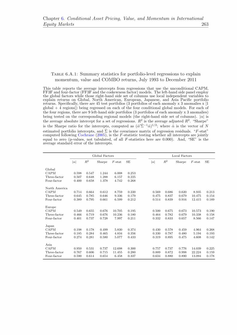
Chapter 6. Conditional Asset Pricing, Value, and Momentum in InternationalEquity Markets 263
Table 6.A.1: Summary statistics for portfolio-level regressions to explainmomentum, value and COMBO returns, July 1993 to December 2011
This table reports the average intercepts from regressions that use the unconditional CAPM,FF3F and four-factor (FF3F and the coskewness factor) models. The left-hand side panel employthe global factors while those right-hand side set of columns use local independent variables toexplain returns on Global, North American, European, Japanese, and Asia Pacific portfolioreturns. Specifically, there are 45 test portfolios (3 portfolios of each anomaly x 3 anomalies x [1global + 4 regions]) being regressed on each of the four conditional global models. For each ofthe four regions, there are 9 left-hand side portfolios (3 portfolios of each anomaly x 3 anomalies)being tested on the corresponding regional models (the right-hand side set of columns). |α| isthe average absolute intercept for a set of regressions. R2 is the average adjusted R2. “Sharpe”is the Sharpe ratio for the intercepts, computed as (α′Σ−1α)1/2; where α is the vector of N
estimated portfolio intercepts, and Σ is the covariance matrix of regression residuals. “F -stat”computed following Cochrane (2005), is the F -statistic testing whether all intercepts are jointlyequal to zero (p-values, not tabulated, of all F -statistics here are 0.000). And, “SE” is theaverage standard error of the intercepts.
Global Factors Local Factors
|α| R2 Sharpe F -stat SE |α| R2 Sharpe F -stat SE
GlobalCAPM 0.598 0.547 1.244 6.008 0.253Three-factor 0.507 0.648 1.288 6.157 0.225Four-factor 0.400 0.658 1.378 4.742 0.268
North AmericaCAPM 0.714 0.664 0.612 8.759 0.220 0.569 0.686 0.620 8.935 0.213Three-factor 0.645 0.785 0.646 9.336 0.179 0.475 0.837 0.679 10.475 0.154Four-factor 0.389 0.795 0.661 6.599 0.212 0.514 0.839 0.916 12.415 0.189
EuropeCAPM 0.549 0.655 0.676 10.705 0.195 0.500 0.675 0.673 10.573 0.190Three-factor 0.466 0.719 0.676 10.236 0.180 0.464 0.782 0.679 10.338 0.158Four-factor 0.401 0.737 0.728 7.997 0.211 0.332 0.833 0.657 8.566 0.147
JapanCAPM 0.198 0.178 0.499 5.830 0.374 0.430 0.578 0.459 4.964 0.268Three-factor 0.185 0.284 0.465 4.834 0.356 0.330 0.787 0.480 5.194 0.193Four-factor 0.274 0.281 0.580 5.077 0.433 0.319 0.895 0.475 4.608 0.142
AsiaCAPM 0.950 0.531 0.737 12.698 0.300 0.757 0.737 0.776 14.039 0.225Three-factor 0.767 0.606 0.715 11.455 0.280 0.889 0.872 0.998 22.224 0.159Four-factor 0.590 0.614 0.654 6.458 0.337 0.634 0.880 0.890 13.094 0.178

Chapter 7
Conclusions and Future Work
7.1 Summary of research
This thesis extends our understanding about momentum effects in equity markets.
In particular, I examine four important issues covering three main streams of
explanations in the literature. The first study investigates the link between market
underreaction to firm-specific news and momentum profits in four regions: the
U.S., Europe, Japan, and Asia Pacific. I find supporting evidence for Hong and
Stein’s (1999) model that momentum returns are driven by underreaction to news
everywhere. The most important contribution of this study is that it is the first
to jointly examine the effects of news tone and staleness. By doing so, I document
a news trading strategy that is profitable everywhere including Japan where the
normal momentum strategy does not work. Those findings are important because
they indicate that investors everywhere have similar bias of underreacting to news.
They are rare empirical support for behavioral models, and more interestingly this
support is robust in all markets. The study also has implications for international
asset pricing, which will have to account for the behavioral aspect of investors in
the model.
264

Chapter 7. Conclusions and Future Work 265
The second study examines the impact of delisted stocks and their delisting returns
on momentum profits in the Australian market. This study is the first to fix the
issue of the lack of delisting returns in Australian data. It also offers alternative
treatments to the problem of non-trading activities, which in turn causes missing
returns in those missing months. This joint examination means that my findings
are internationally comparable to the literature. I find that the delisting effect is
the main driver of momentum returns in the sample of all stocks – consistent with
the U.S. evidence. However, when I limit the sample to the largest 300 stocks by
market capitalization, the delisting effect disappears – in contrast to the U.S.’s
findings. Because the Top300 stocks are the most liquid and accessible to both
institutional and individual investors, I argue that momentum returns in Australia
are more puzzling.
The third study tests whether conditional asset pricing models can explain mo-
mentum returns. I provide strong motivations as to why we should employ the
model to risk adjust returns on individual stock components of momentum port-
folios. I show that the primary advantage of the component-level risk adjustment
comes from (1) its ability to pick up the time varying dynamics of individual win-
ner and loser stocks and (2) its ability to avoid the arbitrary way of sorting stocks
that conceal those time variations at the portfolio level. I find that the condi-
tional FF3F model, when being applied on individual stock returns, can reduce
the average alpha by 50% from the portfolio-level estimate. Moreover, the con-
ditional FF3F model performs better than the conditional CAPM in explaining
momentum profits, in contrast to what we know from the portfolio-level evidence.
The final important contribution is the documentation of the sample selection bias
inherent in existing studies that also use component-level risk adjustment. I show
that this bias comes from the inclusion of ranking period returns in the estimation.
After correcting for this bias, the results of Chordia and Shivakumar (2002) are
overturned.

Chapter 7. Conclusions and Future Work 266
The fourth study investigates whether the methodology of component-level risk
adjustments in the previous Chapter can explain momentum, value, and Asness
et al.’s (2013) COMBO returns in four regions: North America, Europe, Japan,
and Asia Pacific (23 developed markets). The results confirm that this methodol-
ogy improves the explanatory power of conditional asset pricing models in every
country. Using the new test method, I also offer a new perspective to the debate
of whether international asset pricing is integrated across regions.
As suggested by the literature, I hypothesize that some stocks such as those of
large international companies are more integrated than small local stocks, and
this market integration is time-varying. Consequently, the component-level risk
adjustment can pick up this time variation because conditional asset pricing mod-
els are applied on individual components’ returns, thereby allowing global models
to have the highest explanatory power on globally integrated stocks. Consistent
with this hypothesis, I find that markets are integrated in North America, Japan,
and Asia Pacific – in contrast to the portfolio-level evidence. But similar to the
portfolio-level evidence, the local risk factors still have lower average pricing er-
rors in Europe. These findings, which are consistent with the prediction of inter-
national asset pricing theories, suggest that there are some common risk factors
driving international stock returns, which can be detected by looking at the risk
of individual stock components.
7.2 Limitations and future research
As acknowledged in Chapter 3, although the modern news analytics technology
of TRNA is advanced over the existing research, it is limited to analyzing English
news. This limitation is especially problematic in non-English speaking countries
such as Japan. Consequently, if one believes that investors in Japanese markets
do not read English news then my findings can be driven by the trading activity of

Chapter 7. Conclusions and Future Work 267
foreign investors. Although it is hard to believe that multinational companies and
mutual funds in Japan do not follow English news, this question of who trades on
news is still an ongoing debate in the literature. The literature does not settle on
which type of investors (domestic versus foreign investors and individual versus
institutional investors) actually trades on news and thereby drives momentum
returns. In order to answer these questions, we need the data of investors’ trading
activities, which is not available to me. With the increasing availability of quality
news database, I believe that these questions are the next logical step of future
research.
In Chapter 4, readers may correctly point out that I do not solve the puzzle but
further raise the puzzling fact about momentum effects in the Australian Top300
stocks. However, the purpose of my study is to investigate whether delisted stocks
and their delisting returns are the primary driver of momentum returns outside the
dominant U.S. markets. My conclusion is that, in contrast to the U.S.’s findings
(Eisdorfer, 2008), they are not the explanation in the Australian equity market.
It is beyond the scope of this study to further examine other explanations of
momentum – an ongoing debate as pointed out in Chapter 2. The implication for
future Australian research is that researchers can limit their sample to the Top300
stocks to test behavioral and rational theories. The Australian Top300 is also a
good out-of-sample test for any successful explanations of momentum returns in
the dominant U.S. literature.
In Chapters 5 and 6, although I show that some common asset pricing models
perform well in explaining momentum, value, and COMBO returns, they still
cannot fully explain all anomalies. One limitation is the bad model specification;
there are some other risk factors that we do not observe or test. This research on
the specification of a unified asset pricing model is one of the most active debates
in the finance literature, with more than 50 risk factors being proposed and used
to explain stock returns (Subrahmanyam, 2009). Nevertheless, future research

Chapter 7. Conclusions and Future Work 268
can apply this methodology to test other important risk factors such as liquidity
risk (Sadka, 2006). Moreover, because a good model should be able to explain all
anomalies, we can also use this methodology to explain other financial anomalies
such as accruals (Sloan, 1996).

Bibliography
Ahern, K. R. and Sosyuara, D. (2013). Who writes the news? Corporate press
release during merger negotiations. The Journal of Finance, forthcomming.
Altman, E. (1968). Financial ratios, discriminant analysis and the prediction of
corporate bankruptcy. The Journal of Finance, 23:589–609.
Ang, A. and Bekaert, G. (2002). International asset allocation with regime shifts.
Review of Financial Studies, 15:1137–1187.
Ang, A., Liu, J., and Schwarz, K. (2010). Using stocks or portfolios in tests of
factor models. NBER Working Paper.
Antoniou, C., Doukas, J. A., and Subrahmanyam, A. (2013). Cognitive dissonance,
sentiment, and momentum. Journal of Financial and Quantitative Analysis,
48(1):245–275.
Antweiler, W. and Frank, M. Z. (2004). Is all that talk just noise? The information
content of Internet stock messages boards. The Journal of Finance, 59:1259–
1293.
Antweiler, W. and Frank, M. Z. (2006). Do U.S. stock markets typically overreact
to corporate news stories? Working Paper, University of British Columbia.
Asness, C. S., Moskowitz, T. J., and Pedersen, L. H. (2013). Value and momentum
everywhere. The Journal of Finance, LXVIII.
269

Bibliography 270
Avramov, D., Chordia, T., Jostova, G., and Philipov, A. (2007). Momentum and
credit rating. The Journal of Finance, 62:2503—20.
Badrinath, S. G. and Walhal, S. (2002). Momentum trading by institutions. The
Journal of Finance, 57:2449–2478.
Bailey, W., Karolyi, G., and Salva, C. (2006). The economic consequences of
increased disclosure: Evidence from international cross-listings. Journal of Ac-
counting and Economics, 81:175–213.
Baker, M. and Wurgler, J. (2006). Investor sentiment and the cross-section of
stock returns. The Journal of Finance, 61:1645—80.
Baker, M. and Wurgler, J. (2007). Investor sentiment in the stock market. Journal
of Economic Perspectives, 21(129—52).
Ball, R. and Kothari, S. P. (1991). Security returns around earnings annoucements.
The Accounting Review, 66:718–738.
Bandarchuk, P. and Hilscher, J. (2013). Sources of momentum profits: Evidence
on the irrelevance of characteristics. Review of Finance, 17:809–845.
Barber, B. and Odean, T. (2008). All that glitters: The effect of attention and
news on the buying behavior of individual and institutional investors. Review
of Financial Studies, 21(2):785–818.
Barber, B. M. and Loeffler, D. (1993). The “dartboard” column: Second-hand
information and price pressure. The Journal of Financial and Quantitative
Analysis, 28:273–284.
Barber, B. M. and Lyon, J. D. (1997). Detecting long-run abnormal stock returns:
the empirical power and specification of test statistics. Journal of Financial
Economics, 97:341–72.

Bibliography 271
Barberis, N., Shleifer, A., and Vishny, R. (1998). A model of investor sentiment.
Journal of Financial Economics, 49(207–43).
Beaver, W., McNichols, M., and Price, R. (2007). Delisting returns and their effect
on accounting-based market anomalies. Journal of Accounting and Economics,
43:341–368.
Bekaert, G. and Harvey, C. R. (1995). Time-varying world market integration.
The Journal of Finance, 50:403–444.
Berkowitz, S. A., Logue, D. E., and Noser, E. A. J. (1988). The total costs of
transactions on the nyse. The Journal of Finance, 43:97–112.
Bettman, J. L., Maher, T. R. B., and Sault, S. J. (2009). Momentum profits in
the Australian equity market: a matched firm approach. Pacific-Basin Finance
Journal, 17:565–79.
Bhattacharya, U., Daouk, H., Jorgenson, B., and Kehr, C. (2000). When an event
is not an event: The curious case of an emgerging market. Journal of Financial
Economics, 55:69–101.
Boguth, O., Carlson, M., Fisher, A., and Simutin, M. (2011). Conditional risk and
performance evaluation: Volatility timing, overconditioning, and new estimates
of momentum alphas. Journal of Financial Economics, 102:363–89.
Boudoukh, J., Feldman, R., Kogan, S., and Richardson, M. (2012). Which news
moves stock prices? A textual analysis. NBER Working Paper.
Boudoukh, J., Richardson, M., and Whitelaw, R. F. (1994). Industry returns and
the fisher effect. The Journal of Finance, 49:1595–1615.
Brailsford, T., Gaunt, C., and O’Brien, M. A. (2008). Size and book-to-market
factors in Australia. 21st Australasian Finance and Banking Conference.
Bibliography 272
Brailsford, T. and O’Brien, M. A. (2008). Disentangling size from momentum in
Australian stock returns. Australian Journal of Management, 33(Special Issue).
Chan, W. S. (2003). Stock price reaction to news and no-news: Drift and reversal
after headlines. Journal of Financial Economics, 70:223–260.
Chordia, T., Goyal, A., and Shanken, J. (2011). Cross-sectional asset pricing with
individual stocks. Goizueta Business School, Emory University Working Paper
Series.
Chordia, T. and Shivakumar, L. (2002). Momentum, business cycle, and time-
varying expected returns. The Journal of Finance, LVII:985–1019.
Chui, A. C., Titman, S., and Wei, K. C. J. (2010). Individualism and momentum
around the world. The Journal of Finance, 65:361–292.
Chui, A. C., Wei, C. W., and Titman, S. (2009). Individualism and momentum
around the world. The Journal of Finance, -:2143–84.
Chui, A. C., Wei, K. C., and Titman, S. (2000). Momentum, legal systems and
ownership structure: an analysis of asian stock markets. SSRN.
Cochrane, J. H. (2005). Asset pricing. 2nd edition, Princeton University Press,
Princeton.
Comerton-Forde, C., Gallagher, D. R., Nahhas, J., and Walter, T. S. (2010).
Transaction costs and institutional trading in small-cap equity funds. Australian
Journal of Management, 35:313–27.
Conrad, J., Dittmar, R. F., and Ghysels, E. (2012). Ex ante skewness and expected
stock returns. The Journal of Finance, forthcomming.
Conrad, J. and Kaul, G. (1998). An anatomy of trading strategies. Review of
Financial Studies, 11:489–519.

Bibliography 273
Cooper, M. J., JR., R. C. G., and Hameed, A. (2004). Market states and momen-
tum. The Journal of Finance, LIX:1345–66.
Daniel, K., Hirshleifer, D., and Subrahmanyam, A. (1998). Investor psychology
and security market under- and overreactions. The Journal of Finance, 53:369–
403.
Daniel, K. and Moskowitz, T. (2011). Momentum crashes. NBER Working Paper.
Daniel, K. and Titman, S. (1999). Market efficiency in an irrational world. Fi-
nancial Analysts Journal, 55:28–40.
Das, S. and Chen, M. (2007). Yahoo! for Amazon: Opinion extraction from small
talk on the web. Management Science, 53:1375–88.
Davies, P. L. and Canes, M. (1978). Stock prices and the publication of second-
hand information. The Journal of Business, 51:43–56.
Davis, A. K., Piger, J., and Sedor, L. M. (2012). Beyond the numbers: an analysis
of optimistic and pessimistic language in earnings press releases. Contemporary
Accounting Research, 29:845–68.
DeFond, M., Hung, M., and Trezevant, R. (2007). Investor protection and the
information content of annual earnings annoucements: International evidence.
Journal of Accounting and Economics, 43:37–67.
DeLong, J. B., Shleifer, A., Summers, L., and Waldmann, R. J. (1990). Noise
trader risk in financial markets. Journal of Political Economy, 98:703–738.
Demir, I., Muthuswamy, J., and Walter, T. (2004). Momentum returns in Aus-
tralian equities: the influence of size, risk, liquidity and return computation.
Pacific-Basin Finance Journal, 12:143–58.
Dempsey, M. (2010). The book-to-market equity ratio as a proxy for risk: evidence
from Australian market. Australian Journal of Management, 35:7–21.
Bibliography 274
Dittmar, R. F. (2002). Non-linear pricing kernels, kurtosis preference and evidence
from the cross section of equity returns. The Journal of Finance, 57:369–403.
Dumas, B. and Solnik, B. (1995). The world price of foreign exchange risk. The
Journal of Finance, 50:455–79.
Durand, R. B., Limkriangkrai, M., and Smith, G. (2006a). In America’s thrall:
the effects of the US market and US security characteristics on Australian stock
returns. Accounting and Finance, pages 577–604.
Durand, R. B., Limkriangkrai, M., and Smith, G. (2006b). Momentum in Australia
– A note. Australian Journal of Management, 31:355–64.
Dzielinski, M. (2011). News sensitivity and the cross section of stock returns.
Working Paper, University of Zurich.
Eisdorfer, A. (2008). Delisted firms and momentum profits. Journal of Financial
Markets, 11:160–179.
Engelberg, J. (2008). Costly information processing: Evidence from earnings an-
noucements. Working Paper, University of North Carolina.
Faff, R. (2004). A simple test of Fama and French model using daily data: Aus-
tralian evidence. Applied Financial Economics, 14:83–92.
Fama, E. and French, K. R. (1989). Business conditions and expected returns on
stocks and bonds. Journal of Financial Economics, 25:23–49.
Fama, E. and French, K. R. (1992). The cross section of expected stock returns.
Journal of Financial Economics, 47:427–465.
Fama, E. and French, K. R. (1993). Common risk factors in the returns on stocks
and bonds. Journal of Financial Economics, 33:3–56.
Fama, E. and French, K. R. (1996). Multifactor explanations of asset pricing
anomalies. The Journal of Finance, 51:55–84.

Bibliography 275
Fama, E. F. (1970). Efficient capital markets: A review of theory and empirical
work. The Journal of Finance, 25:383–417.
Fama, E. F. (1998). Market efficiency, long-term returns, and behavioral finance.
Journal of Financial Economics, 49:283–306.
Fama, E. F. and French, K. R. (1998). Value versus growth: The international
evidence. The Journal of Finance, 53:1975–1999.
Fama, E. F. and French, K. R. (2008). Dissecting anomalies. The Journal of
Finance, LXIII:1653–79.
Fama, E. F. and French, K. R. (2012). Size, value, and momentum in international
stock returns. Journal of Financial Economics, 105:457–72.
Fama, E. F. and Litterman, R. (2012). An experienced view on markets and
investing. Financial Analysts Journal, 68:1–5.
Fama, E. F. and MacBeth, J. D. (1973). Risk, return and equilibrium: Empirical
tests. Journal of Political Economy, 81:607–636.
Fang, L. and Peress, J. (2009). Media coverage and the cross-section of stock
returns. The Journal of Finance, 64:2023–52.
Ferson, W., Simin, T., and Sarkissian, S. (2008). Asset pricing models with con-
ditional alphas and betas: the effects of data snooping and spurious regression.
Journal of Financial and Quantitative Analysis, 43:331–354.
Ferson, W. E. and Harvey, C. R. (1993). The risk and predictability of international
equity returns. The Review of Financial Studies, 6:527–566.
Ferson, W. E. and Harvey, C. R. (1999). Conditioning variables and the cross
section of stock returns. The Journal of Finance, 54:1325–60.
Ferson, W. E. and Schadt, R. W. (1996). Measuring fund strategy and performance
in changing economic conditions. The Journal of Finance, 51:425–461.

Bibliography 276
Galariotis, C. E. (2010). What should we know about momentum investing?
The case of the Australian Security Exchange. Pacific-Basin Finance Journal,
18:369–89.
Garcia, D. (2013). Sentiment during recessions. The Journal of Finance, 68:1267–
1300.
Gibbons, M. R., Ross, S. A., and Shanken, J. (1989). A test of the efficiency of a
given portfolio. Econometrica, 57:1121–52.
Goyal, A. and Welch, I. (2008). A comprehensive look at the empirical performance
of equity premium prediction. Review of Financial Studies, 21:1455–1580.
Grauer, F. L. A., Litzenberger, R. H., and Stehle, R. E. (1976). Sharing rules
and equilibrium in an international capital market under uncertainty. Journal
of Financial Economics, 3:233–256.
Gray, P. (2013). Stock weighting and nontrading bias in estimated portfolio re-
turns. Accounting and Finance, Advanced Access.
Griffin, J. M. (2002). Are the Fama and French factors global or country specific?
Review of Financial Studies, 15:783–803.
Griffin, J. M., Hirschey, N. H., and Kelly, P. J. (2011). How important is the
financial media in global makets. Review of Financial Studies, 24:3941–93.
Griffin, J. M., Ji, X., and Martin, J. S. (2003). Momenum investing and business
cycle risk: evidence from pole to pole. The Journal of Finance, 58:2515–47.
Griffin, J. M., Ji, X., and Martin, J. S. (2005). Global momentum strategies, a
portfolio perspective. Journal of Portfolio Management, winter.
Griffin, J. M., Kelly, P. J., and Nardari, F. (2010). Do market efficiency measures
yield correct inferences? A comparison of developed and emerging markets.
Review of Financial Studies, 23:3225–3277.

Bibliography 277
Grinblatt, M. and Keloharju, M. (2000). The investment behavior and performance
of various investor types: A study of Finland’s unique dataset. Journal of
Financial Economics, 55:43–67.
Grinblatt, M. and Moskowitz, T. J. (2004). Predicting stock price movements from
past returns: the role of consistency and tax-loss selling. Journal of Financial
Economics, 71:541–79.
Grinblatt, M., Titman, S., and Wermers, R. (1995). Momentum investment strate-
gies, portfolio performance, and herding: A study of mutual fund behavior. The
Ameriance Economic Review, 85:1088–1105.
Grundy, B. D. and Martin, J. S. (2001). Understanding the nature of the risks
and the source of the rewards to momentum investing. The Review of Financial
Studies, 14:29–78.
Gutierrez, R. and Kelly, E. K. (2008). The long-lasting momentum in stock returns.
The Journal of Finance, LXIII(1):415–448.
Halliwell, J., Heaney, R., and Sawicki, J. (1999). Size and book to market effects in
Australian share markets: a time series analysis. Accounting Research Journal,
12:122–37.
Hamilton, J. D. (1989). A new approach to the economic analysis of non-stationary
time series and the business cycle. Econometrica, 57:357–384.
Hamilton, J. D. (1994). Time Series Analysis. Princeton University Press.
Hand, J. R. M. (1990). A test of the extended functional fixation hypothesis. The
Accounting Review, 65:740–763.
Harvey, C. R. (1991). The world price of covariance risk. Journal of Finance,
46:111–157.

Bibliography 278
Harvey, C. R. and Siddique, A. (2000). Conditional skewness in asset pricing. The
Journal of Finance, 34:465–477.
Healy, A. D. and Lo, A. W. (2011). Managing real-time risks and returns: The
Thomson Reuters NewsScope event indicies. Handbook of News Analytics in
Finance, John Wiley & Sons, pages 73–108.
Hofstede, G. (1980). Culture’s consequences: International differences in work-
related values. Sage Publication, Beverly Hills, CA.
Hofstede, G. (2001). Culture’s consequences: comparing values, behaviors, insti-
tutions, and organizations across nations. Sage Publication, Beverly Hills, CA.
Hong, H., Lim, T., and Stein, J. C. (2000). Bad news travels slowly: Size, analyst
coverage, and the profitability of momentum strategies. The Journal of Finance,
LV:265–295.
Hong, H. and Stein, J. C. (1999). A unified theory of underreaction, momentum
trading, and overreaction in asset markets. The Journal of Finance, 54:2143–84.
Hou, K., Karolyi, G. A., and Kho, B. C. (2011). What factors drive global stock
returns? Review of Financial Studies, 24:2528–74.
Hurn, S. and Pavlov, V. (2003). Momentum in Australian stock returns. Australian
Journal of Management, 28:141–56.
Hvidkjaer, S. (2006). A trade-based analysis of momentum. Review of Financial
Studies, 19(2):457–491.
Ince, O. S. and Porter, R. B. (2006). individual equity return data from thomson
datastream: Handle with care! Journal of Financial Research, 29:463–79.
Israel, R. and Moskowitz, T. J. (2013). The role of shorting, firm size, and time
on market anomalies. Journal of Financial Economics, 108:275–301.
Bibliography 279
Jaganathan, R. and Wang, Z. (1996). The conditional capm and the cross section
of expected returns. The Journal of Finance, 51:3–53.
Jegadeesh, N. (1990). Evidence of predictable behavior of security returns. The
Journal of Finance, 45:881–98.
Jegadeesh, N. and Titman, S. (1993). Returns to buying winners and selling losers:
implications for stock market efficiency. The Journal of Finance, 48:65–91.
Jegadeesh, N. and Titman, S. (2001). Profitability of momentum strategies: an
evaluation of alternative explanations. The Journal of Finance, 56:699–720.
Jegadeesh, N. and Titman, S. (2002). Cross-sectional and time-series determinants
of momentum returns. The Review of Financial Studies, 15:143–157.
Jegadeesh, N. and Titman, S. (2011). Momentum. The Annual Review of Financial
Economics, 3:493–509.
Karolyi, A. and Wu, Y. (2012). The role of investability restrictions on size, value,
and momentum in international stock returns. Cornell University Working Pa-
per Series.
Karolyi, G. A. and Stulz, R. M. (2003). Are financial assets priced locally or
globally? Chapter 16, Handbook of the Economics and Finance, Edited by
G.M. Constantinides, M. Harris and R. Stulz, Elsevier B. V.
Keim, D. B. and Madhavan, A. (1997). Transaction costs and investment style:
an inter-exchange analysis of institutional equity trades. Journal of Financial
Economics, 46:265–292.
Kim, C.-J., Morley, J. C., and Nelson, C. (2001). Does an intertemporal tradeoff
between risk and return explain mean reversion in stock prices? Journal of
Empirical Finance, 8:403–426.

Bibliography 280
Korajczyk, A. R. and Sadka, R. (2004). Are momentum profits robust to trading
costs? The Journal of Finance, 59:1039–1082.
Kraus, A. and Litzenberger, R. H. (1976). Skewness preference and the valuation
of risk assets. The Journal of Finance, 31:1085–1100.
Lakonishok, J., Shleifer, A., and Vishny, R. W. (1994). Contrarian investment,
extrapolation, and risk. The Journal of Finance, 49:1541–1578.
Lee, C. and Swaminathan, B. (2000). Price momentum and trading volume. The
Journal of Finance, 55:1217–69.
Lesmond, D. A., Schill, M. J., and Zhou, C. (2004). The illusory nature of mo-
mentum profits. Journal of Financial Economics, 71:349–80.
Lettau, M. and Ludvigson, S. C. (2001). Resurrecting the (C )CAPM: A cross-
sectional test when risk premia are time-varying. Journal of Political Economy,
109:1238–87.
Lewellen, J., Nagel, S., and Shanken, J. (2010). A skeptical appraisal of asset
pricing tests. Journal of Financial Economics, 96:175 – 194.
Lewellen, J. S. and Nagel, S. (2006). The conditional CAPM does not explain
asset-pricing anomalies. Journal of Financial Economics, 82:289–314.
Li, F. (2010). The determinants and information content of the forward-looking
statements in corporate filings – a Naive Bayesian machine learning approach.
Journal of Accounting Research, 48:1049–1102.
Lintner, J. (1965). The valuation of risk assets and the selection of risky invest-
ments in stock portfolios and capital budgets. The Review of Economics and
Statistics, 47:13–37.
Liu, L. Z. and Zhang, L. (2008). Momentum profits, factor pricing, and macroe-
conomic risk. Review of Financial Studies, 21:2417–48.

Bibliography 281
Lo, W. A. and MacKinlay, A. C. (1990a). Data-snooping biases in tests of financial
asset pricing models. The Review of Financial Studies, 3:431–67.
Lo, W. A. and MacKinlay, A. C. (1990b). When are contrarian profits due to
stock market overreaction? The Review of Financial Studies, 3:175–205.
Loughran, T. and McDonald, B. (2011). When is a liability not a liability? Textual
analysis, dictionaries, and 10-Ks. The Journal of Finance, LXVI(1):35–65.
Mitra, G. and Mitra, L., editors (2011). The Handbook of News Analytics in
Finance. John Wiley & Sons Ltd.
Moskowitz, T. J. and Grinblatt, M. (1999). Do industries explain momentum?
The Journal of Finance, 54:1249–1290.
Newey, W. K. and West, K. D. (1987). A simple, positive semi-definite, het-
eroskedasticity and autocorrelation consistent covariance matrix. Econometrica,
55:703–708.
Odean, T. (1998). Are investors reluctant to realize their losses? The Journal of
Finance, 53:1775–98.
Rapach, D. E., Strauss, J. K., and Zhou, G. (2013). International stock return
predictability: What is the role of the United States? The Journal of Finance,
LXVIII:1633–1662.
Roll, R. (1984). A simple implicit measure of the effective bid-ask spread in an
efficient market. The Journal of Finance, 39:1127–39.
Rosenberg, B., Reid, K., and Lanstein, R. (1985). Persuasive evidence of market
inefficiency. Journal of Portfolio Management, 11:9–15.
Rouwenhorst, K. G. (1998). International momentum strategies. The Journal of
Finance, 53:267–84.

Bibliography 282
Rouwenhorst, K. G. (1999). European equitiy markets and the emu. Financial
Analysts Journal, 55:57–64.
Sadka, R. (2006). Momentum and post-earnings-announcement drift anomalies:
The role of liquidity risk. Journal of Financial Economics, 80:309–49.
Sagi, J. S. and Seasholes, M. S. (2007). Firm specific attributes and the cross-
section of momentum. Journal of Financial Economics, 84:389–434.
Scowcroft, A. and Sefton, J. (2005). Understanding momentum. Financial Ana-
lysts Journal, 55:57–64.
Shanken, J. (1990). Intertemporal asset pricing: An emperical investigtation.
Journal of Econometrics, 45:99–120.
Sharpe, W. F. (1964). Capital asset prices: a theory of market equilibrium under
conditions of risk. The Journal of Finance, 19:425–442.
Shumway, T. (1997). The delisting bias in crsp data. The Journal of Finance,
52:327–340.
Shumway, T. and Warther, V. (1999). The delisting bias in crsp’s nasdaq data
and its implications for the size effect. Journal of Finance, 54:2361–2389.
Sinha, N. R. (2012). Underreaction to news in the US stock market. Working
Paper, University of Illinois at Chicago.
Sloan, R. G. (1996). Do stock prices fully reflect information in accruals and cash
flows about future earnings. The Accounting Review, 71:289–315.
Smith, D. R. (2007). Conditional coskewness and asset pricing. Journal of Em-
perical Finance, 14:91–119.
Stattman, D. (1980). Book values and stock returns. Chicago MBA: A Journal of
Selected Papers, 5:25–45.

Bibliography 283
Stivers, C. and Sun, L. (2010). Cross-sectional return dispersion and time-variation
in value and momentum premia. The Journal of Financial and Quantitative
Analysis, 45:987–1014.
Stulz, R. M. (1995). The cost of capital in internationally integrated markets: The
case of Nestle. European Financial Management, 1:11–22.
Subrahmanyam, A. (2009). The cross-section of expected stock returns: What
have we learnt from the past twenty-five years of research? UCLA Working
Paper Series.
Tetlock, P. (2007). Giving content to investor sentiment: The role of media in the
stock market. The Journal of Finance, LXII:1139–69.
Tetlock, P. (2011). All the news that’s fit to reprint: Do investors react to stale
information? Review of Financial Studies, 24:1481–1513.
Tetlock, P., Saar-Tsechansky, M., and Macskassy, S. (2008). More than words:
Quantifying language to measure firms’ fundamentals. The Journal of Finance,
LXIII:1437–69.
Turner, C. M., Starz, R., and Nelson, C. R. (1989). A markov model of het-
eroskedasticity, risk and learning in the stock market. Journal of Financial
Economics, 25:3–22.
Vasicek, O. A. (1973). A note on using cross-sectional information in Bayesian
estimation of security betas. The Journal of Finance, 28:1233–39.
Wang, J. and Wu, Y. (2011). Risk adjustment and momentum sources. Journal
of Banking and Finance, 35:1427–1435.
Wang, K. Q. and Xu, J. (2010). Time-varying momentum profitability. SSRN
Working Paper, University of Toronto Working Paper Series.

Bibliography 284
Yao, Y. (2012). Momentum, contrarian, and the january seasonality. Journal of
Banking and Finance, 36:2757–2769.
Zhang, X. F. (2006). Information uncertainty and stock returns. The Journal of
Finance, 61:105–37.