essays on the empirical modelling of money … · essays on the empirical modelling of money demand...
TRANSCRIPT
ESSAYS ON THE EMPIRICAL MODELLING OF MONEY DEMAND IN
PERIODS OF FINANCIAL LIBERALISATION: THE CASE OF INDONESIA
Thesis subm itted for the deg ree of
Doctor of Philosophy
a t th e University of Leicester
by
Gregory A. Jam es
D epartm en t of Economics
University of Leicester
June 2007

UMI Number: U230993
All rights reserved
INFORMATION TO ALL USERS The quality of this reproduction is dependent upon the quality of the copy submitted.
In the unlikely event that the author did not send a complete manuscript and there are missing pages, these will be noted. Also, if material had to be removed,
a note will indicate the deletion.
Dissertation Publishing
UMI U230993Published by ProQuest LLC 2013. Copyright in the Dissertation held by the Author.
Microform Edition © ProQuest LLC.All rights reserved. This work is protected against
unauthorized copying under Title 17, United States Code.
ProQuest LLC 789 East Eisenhower Parkway
P.O. Box 1346 Ann Arbor, Ml 48106-1346

ii
To my wife, Rahayu, and my son, Harry

B ut I shall let the little I have learnt go forth into the day in order that someone
better than I may guess the truth, and in his work may prove and rebuke my error.
A t this I shall rejoice that I was yet a means whereby such truth has come to light.
Albrecht Dtirer

A BSTRA CT
Financial liberalisa tion is widely blam ed for the instability of em pirical money dem and models. A stab le money dem and function (MDF) is a key element in the form ulation of m onetary policy. S tructu ral breaks brought abou t by financial liberalisation can im pair the predictability of the im pact of changes in money on income, the price level and the interest ra te , and render m onetary policy less reliable. This in tu rn can affect individuals’ expectations about fu tu re policy and u ltim ately alter th e effects of a given policy m easure. Thus, obtain ing reliable estim ates of th e param eters of the M D F—through an appropriate m odelling strategy th a t takes into account th e structu ral change induced by financial liberalisation—is a crucial task.
This thesis contains three essays on th e em pirical modelling of money dem and in periods of financial liberalisation. The em pirical analysis uses a quarterly time- series da tase t on Indonesian money, ou tpu t, price, interest and exchange rates from 1983:1 to 2001:4. T he first essay uses a univariate m ethod to identify endogenous s tru c tu ra l breaks in money and th e determ inants of money dem and. The second essay extends th is approach to the m ultivariate case to de tec t endogenous regime shifts in m oney demand. The th ird essay explicitly controls for financial liberalisation in th e M DF.
We find evidence of a break occurring in th e second quarter of 1991 and coinciding w ith a m ajo r government intervention in the money m arket known as the Sum arlin shock. W e also find evidence of a break occurring in th e last quarte r of 1997 and coinciding w ith the severe economic crisis and a governm ent intervention in th e money m arke t for which the Sum arlin shock of 1991 is th e precedent. F inally, we show how m odelling financial liberalisation as a determ inistic drift process constitu tes an im provem ent over the s tandard specifications in term s of yielding more constant and plausible values for th e param eters of the M DF.

ACKNOW LEDGM ENTS
I am deeply indebted to my supervisor, Prof. Wojciecli C harem za, for his invaluable expertise and continuous support. I doubt I will ever b e able to convey my appreciation fully. I would also like to th an k the other m em bers of my thesis com m ittee, Prof. Kevin Lee, and Prof. G ianni De Fraja, for th e assistance they provided a t all levels during the course of th is research. I am deeply indebted to Prof. Panicos Dem etriades, for giving me th e opportunity to jo in this departm ent, and for his continuous support and invaluable advice. I th a n k Prof. Subrat a G hatak from K ingston University for taking tim e out of his busy schedule to serve as my external exam iner. I thank Dr. Ali al-Nowaihi, for his form idable kindness and encouragem ent. Many thanks to Prof. David Fielding, and to all my colleagues in Leicester, for all the instances in which they helped m e along the way. I acknowledge th a t th is research would not have been possible w ith o u t the financial assistance of the D epartm ent of Economics a t the University of Leicester (G raduate Teaching A ssistantship, PhD Scholarship). Finally, I thank m y parents, A nna and Michel, for th e support they provided me through my entire life. M ost of all, I thank my wife, R ahayu, and my son, Harry, w ithout whose love and patience, I would not have finished this thesis. Tesis ini bagi anda berdua, salarn sayang.

CONTENTS
A B ST R A C T .......................................................................................................... iv
ACKNOW LEDGM ENTS................................................................................. v
LIST OF TABLES.............................................................................................. ix
LIST OF FIG URES............................................................................................. x
Chapter
1 INTR O D UC TIO N ......................................................................................... 1
2 A REVIEW OF THEORIES AND EMPIRICAL MODELS OF MONEY D E M A N D ................................................................................... 7
2.1 Economic theories of money d e m a n d ........................................................... 72.2 Econometric fo rm u la tio n s ............................................................................... 172.3 Financial liberalisation, stationarity and structural stability of MDFs . 31
3 AN OVERVIEW OF FINANCIAL LIBERALISATION IN IND O N E SIA ........................................................................................................ 37
3.1 Banking system r e f o r m s .................................................................................. 383 . 2 Capital market re fo rm s...................................................................................... 473.3 Changes in monetary p o l i c y ............................................................................ 553.4 Crisis-driven reforms and policy c h a n g e s ...................................................... 60
4 FINANCIAL LIBERALISATION AND STRUCTURAL BREAKS IN MONETARY AGGREGATES AND THE DETERM INANTS OF MONEY DEM AND IN IN D O N ESIA ........................................... 66
4.1 In tro d u c tio n .......................................................................................................... 6 6
4.2 M e th o d o lo g y ....................................................................................................... 6 8
4.3 Empirical r e s u l t s ................................................................................................ 724.4 C o n c lu sio n s .......................................................................................................... 78

5 FINANCIAL LIBERALISATION AND REGIME SHIFTS IN INDONESIAN MONEY D E M A N D ............................................................ 88
5.1 In tro d u c tio n ......................................................................................................... 8 8
5.2 Methodology ...................................................................................................... 905.3 Empirical r e s u l t s ............................................................................................... 965.4 C o n c lu sio n s .............................................................................................................115
6 ARDL APPROACH TO MODELLING INDONESIAN MONEY DEM AND W ITH FINANCIAL LIBERALISATION......................... 119
6.1 In tro d u c tio n .............................................................................................................1196.2 Methodology ......................................................................................................... 1216.3 Empirical r e s u l t s ...................................................................................................1246.4 C o n c lu sio n s............................................................................................................. 135
7 CONCLUSION.......................................................................................... 137
REFER ENCES................................................................................................... 141

LIST OF TABLES
3.1 Share issues by listed companies, 1990-2001 ............................................... 52
3.2 Trading value of listed shares on the JSX by type of investor, 1992-2001 53
3.3 JSX, yearly statistics, 1983-2001 ...................................................................... 5 4
3.4 JSX, yearly (end-period) composite share price index, 1983-2001 . . . . 56
4.1 IO Model 2 results . ....................................................................................... 76
4.2 IO Model 2 results (continued) ....................................................................... 77
4.3 IO Model 2 results (continued) ....................................................................... 79
4.4 Leybourne (1995) unit root tests ................................................................... 80
4.5 AO Model 2 r e s u l ts .............................................................................................. 85
4.6 AO Model 2 results (co n tin u ed )....................................................................... 8 6
4.7 AO Model 2 results (co n tin u ed )....................................................................... 87
5.1 Augmented Dickey-Fuller and Phillips-Perron tests: Indonesian money
dem and d a ta (1986:1-2001:4), seasonaly adjusted .............................. 94
5.2 Augmented Dickey-Fuller and Phillips-Perron tests (con tinued)............. 95
5.3 Dickey-Fuller GLS de-trended and Ng-Perron tests: Indonesian money
dem and d a ta (1986:1-2001:4), seasonaly adjusted .............................. 97
5.4 Dickey-Fuller GLS de-trended and Ng-Perron tests (con tinued )............. 98
5.5 Indonesian money demand model evaluation diagnostics, 1989:1-2001:4 100
viii

5.6 Indonesian money demand model evaluation diagnostics (continued) . . 101
5.7 Indonesian money demand model evaluation diagnostics when dummy
variables are inc luded ....................................................................................... 1 0 2
5.8 Test of the cointegration rank of the Indonesian money dem and model,
unrestricted intercepts and no trends, 1989:1-2001:4 ........................... 106
5.9 Determining cointegration rank and the model for the deterministic
components using the trace test, Indonesian money dem and data,
1989:1-2001:4 .................................................................................................. 107
5.10 Normalised cointegration coefficients of the Indonesian money demand
model, 1989:1-2001:4 .................................................................................... 107
5.11 Test for weak exogeneity of RGDP, MMR, and R E R .............................. 108
5.12 Results of the conditional model, 1989:1-2001:4 ........................................ 110
5.13 Tests of significance of each variable/lag and COMFAC t e s t s .................I l l
5.14 Tests of cointegration with regime s h i f t s ...................................................... 114
6.1 Statistics for selecting the lag order of the Indonesian money demand
e q u a t io n ............................................................................................................... 128
6.2 F-and t- statistics for testing the existence of a long-run money demand
equation for I n d o n e s ia .................................................................................... 130
6.3 U nrestricted error correction model of the Indonesian money demand
e q u a t io n ................................................................................................................132
6.4 U nrestricted error correction model without impulse dumm y variables . 134
LIST OF FIGURES
3.1 Interest and inflation rates, 1980-2000 ............................................................ 42
3.2 M onetary ratios as percentage of GDP, 1983-2000 ..................................... 45
3.3 Im pact of deregulation on bank deposits (outstanding balances as % of
nominal GDP), 1980-2000 ......................................................................... 46
3.4 Key interest rates, 1983-2000 .......................................................................... 61
4.1 Plots of the time series .................................................................................... 73
5.1 Residuals (scaled) and residual densities for RM1, RGDP, MMR, and
RER, lag le n g th = 2 ......................................................................................... 103
5.2 Residuals (scaled) and residuals densities for RM1, RGDP, MMR, and
RER, lag length=2, including Dum97:3, D um98:l, Dum98:2 . . . . 104
5.3 Plots of the v e c to rs .................................................................................................105
5.4 Plots of the vectors, corrected for short-run d y n am ics ..................................106
5.5 Regime shifts with ADF*, Indonesian money demand, 1989:1-2001:4 . . 115
6.1 Plot of actual and fitted values ........................................................................ 133
6.2 Plot of cumulative sum of recursive residuals .................................... 135
6.3 Plot of cumulative sum of squares of recursive re s id u a ls ....................135
x

CHAPTER 1
INTRODUCTION
During the last three decades, substantial changes occurred in the design and
conduct of monetary policy in Indonesia. Before the early 1980s, Indonesia’s cen
tra l bank—like most central banks in the Southeast Asian region—relied on direct
control measures such as interest rate ceilings, minimum reserve requirements, and
exchange rate controls to implement monetary policy. However, in June 1983, the
government embarked upon structural reforms and financial liberalisation which
saw the abolition of interest rate controls, liberalisation of the capital market, and
removal of entry restrictions of foreign banks into the domestic banking market.
The aim was to increase saving and the level and efficiency of investment to sup
port economic growth and achieve higher living standards. In parallel with these
reforms, Indonesia’s central bank started to rely increasingly on market-based mea
sures to implement monetary policy. Following the interest rate liberalisation, the
bank introduced the use of open market operations and started issuing its own
debt instrum ents in the absence of government debt securities. The move was ac
companied by the adoption of monetary targeting as the main framework for the
conduct and implementation of monetary policy.
Implicit in monetary targeting is the notion of a stable money demand function
(Poole, 1970). The existence of a stable and predictable relationship between
monetary aggregates, economic activity, prices and interest rate is key to the theory
and application of macroeconomic policies as it provides a reliable link between
changes in monetary aggregates and changes in the variables included in the money
demand function (Siddiki and Morrissey, 2006; Ericsson, 1998; Ghatak, 1995).
While economic theory supports the notion th a t money demand is likely to be a
stable function of income, prices, and interest rates, this stability is predicated on
an unchanging institutional environment.
One might expect a priori th a t the increasing globalisation of the Indonesian
financial market and institutional changes in the conduct of monetary policy would
have a destabilising impact on the underlying money demand function. The ex
perience of many industrial countries tha t went through substantial episodes of
financial reforms and deregulation during the early and mid-1980s revealed signif
icant shifts in the money demand relationship, which made it difficult to retain
intermediate monetary targets. Financial liberalisation, by improving the qual
ity of economic signals, altering the institutional environment, and expanding the
array of financial opportunities, creates potential for money demand instability.
Interest rates th a t better reflect the return and riskiness of financial assets can
prom pt portfolio shifts in money demand. Measures th a t improve the functioning
of financial markets can prompt portfolio shifts as well as alter the sensitivity of
money to changes in income and interest rates. More generally, measures tha t
promote financial development may result in the availability of new, attractive as
sets (for instance foreign assets if external capital flows are liberalised) leading to
gradual portfolio shifts away from monetary assets (Tseng and Corker, 1991).

Changes in the institutional environment brought about by financial liberali
sation are also widely perceived to be responsible for observed cycles in the income
velocity of money (Bordo and Jonung, 1987; 1990). This places some practical
limits on the notion of stability. In particular, it may be impossible to identify a
stable money demand relationship for all time, but it may be possible to estimate a
relationship for which the key parameters are reasonably constant over the sample
period in question. This would provide some grounds for concluding tha t monetary
developments remain predictable in the future, at least over the duration of the
policy horizon (Tseng and Corker, 1991).
From an econometric perspective, the question of the stability of money de
mand has been intensively investigated using a variety of econometric techniques.
Currently, the most popular framework for examining the behaviour of money de
mand is the cointegration framework. In this framework, the stationarity of money
demand instead of the stability of money demand is evaluated. Earlier tests of the
stability of money demand typically centered on whether the coefficients estimates
were stable, th a t is, not subject to structural breaks (see, for instance, Aghevli et
al., 1979). These tests did not consider the underlying time series aspects of the
variables in money demand or the time series properties of their joint relationship
prior to estimation as is now common in the cointegration framework.
From a policy perspective, finding tha t money demand is nonstationary is
problematic since the ability of policymakers to prevent money market disruptions
depends on whether a money demand relationship th a t is predictable can be iden

tified. If money demand is nonstationary then the monetary authorities may not
be able to use such a relationship to target money growth with accuracy. In such
case, the central bank’s ability ex ante to prevent a money market disequilibria
from affecting the economy could be curtailed. Finding tha t money demand is not
stable is also problematic since proper policy conduct may ex post be misguided
in light of a structural break and there may be a period of learning before policy
is readjusted to its proper course (Breuer and Lippert, 1996).
The issues of stationarity and structural stability, however, should not be
treated independently. It is possible that tests th a t find money demand is nonsta
tionary may be flawed because the estimations procedures used have not considered
a structural break. Failure to take account of structural change may bias the results
in favour of nonstationarity.
The thesis contains three essays on the empirical modelling of money demand
in periods of financial liberalisation: the case of Indonesia. Indonesia, having
experienced financial liberalisation as well as a banking crisis of real gravity, and
given its monetary framework, is a well chosen subject for money demand analysis.
Its population, four times Britain’s, and its strategic significance makes it a country
worthy of study in its own right. However, the Indonesian case also exemplifies
the experiences of structural reforms, policy changes and financial innovations of
many developing countries in Asia and around the world. The methods and key
findings of the thesis should therefore prove useful in improving our understanding
of the effects of structural change on money demand not only for Indonesia but

also for a variety of developing economies.
The empirical analysis uses a quarterly time-series dataset on Indonesian money,
output, price, interest and exchange rates from 1983:1 to 2001:4. Our theoretical
and empirical starting points are provided in chapter 2. We review theories of
money demand and their econometric formulations. We also discuss the implica
tions of financial liberalisation on the stationarity and structural stability of the
money demand function.
In chapter 3 we present an overview of financial liberalisation in Indonesia.
We review significant financial reforms and discuss changes in monetary policy.
We also analyse the development of the financial sector and include quantitative
measures of its growth and structural change.
In chapter 4 we use a univariate method to search for endogenous structural
breaks in m onetary aggregates and the determinants of money demand in Indone
sia. We use the procedure outlined in Vogelsang and Perron (1998). The null
hypothesis is th a t of a unit root against the alternative of stationarity with a
break of unknown timing in the intercept and slope of the trend function of the
series.
In chapter 5, we apply a multivariate method to search for endogenous regime
shifts in Indonesian money demand. We use the cointegration test of Gregory
and Hansen (1996), which allows for a structural break of unknown timing in the
money demand function.
In chapter 6 , the content of which has been published as a journal article:

James, G. A. (2005). ‘Money Demand and Financial Liberalization
in Indonesia.’ Journal of Asian Economics, vol. 16, pp. 817-29.
we explicitly model financial liberalisation as a deterministic drift process.
We follow the ARDL approach of Pesaran, Shin and Smith (2001), which avoids
pretesting of the order of integration of the series in the money demand function.
Finally, we conclude in chapter 7 by assessing the empirical relevance of our
results and discussing their implications for future research.

CHAPTER 2
A REVIEW OF THEORIES AND EMPIRICAL MODELS OF MONEY
DEMAND
The purpose of this chapter is to offer a review of economic theories and econo
metric formulations of the demand for money. From an empirical point of view,
the theoretical literature implies tha t the aggregate demand for money (the money
demanded by households, firms and the government) depends positively on a scale
(transaction) variable; negatively on one or more opportunity costs variables (usu
ally some interest rates and/or the inflation rate). Differences between competing
theories relate to the use of the appropriate scale and opportunity cost variables.
The chapter finishes with a discussion on financial liberalisation and its empirical
implications in term s of structural change and model misspecification.
2.1 Economic theories of money demand
Money serves four major functions—medium of exchange, store of value, unit
of account, and source of deferred payment. Individuals hold money balances for
various reasons—transactions, precaution and speculation. Each money demand
theory places particular emphasis on one or more of these functions and underlying
motives. This following discussion briefly reviews the theoretical literature on
money demand. The reader is referred to Cuthbertson (1985), Goldfeld and Sichel
(1990), and Laidler (1993) for comprehensive surveys.
2 .1 .1 The quantity theory and Keynes’s theory
One early approach to the demand for money is the quantity theory of money, put
forward by Fisher (1911), and the so-called Cambridge economists, Marshall (see
W hitaker, 1975) and Pigou (1917). Both Fisher and the Cambridge economists
are concerned primarily with money as a means of exchange and therefore provide
models of the transactions demand for money.
Fisher (1911) analyses the institutional details of the payments mechanism
and therefore concentrates on the velocity of circulation of money. The basis of
Fisher’s theory is an identity linking the value of sales with the amount of money
which changes hands. If Y equals the volume of transactions and P equals the
average price level then P Y = the value of transactions undertaken. The number
of times the money changes hands, tha t is the velocity of circulation of money V
multiplied by the fixed stock of money M, must be equal to the value of transaction
(M V = P Y ). One crucial assumption is tha t V, being determined by technological
and /or institutional factors, is relatively constant. More specifically, it is assumed
th a t the payments mechanism is such tha t the velocity of circulation is constant
in the short run and varies slowly and in a predictable way in the long-run, as
payments mechanisms in the economy change.
The Cambridge economists are concerned with the determ inants of the indi
vidual’s desired demand for money. Although the transactions motive is still the
main determinant of desired money holdings, they argue th a t one alternative to
holding money is to hold an interest bearing asset called a bond. The higher the

rate of returns on bonds, relative to the marginal utility from money, the more
individuals are encouraged to switch some of their money holdings into bonds.
Assuming a proportionate relationship, one can write M d = K P Y . If one assumes
money market equilibrium then M s = M d = K P Y . Hence V = l / K and since
K depends upon the interest rate and wealth, the Cambridge economists consider
th a t the velocity of circulation is neither constant in the short run nor in the long
run.
Keynes (1936) broadly accepts the view of the Cambridge economists concern
ing the transactions demand for money. He also introduces two other motives
for holding money — precautionary and speculative. The main predictions from
Keynes’s theory are, first, th a t individuals do not hold a diversified portfolio of
assets: they would hold either all bonds or all money. Second, there is a downward
slopping aggregate demand for money function with respect to the interest rate.
Finally, the theory predicts the possibility of a liquidity trap, meaning tha t under
certain circumstances, the interest elasticity of the demand for money can become
infinite. Keynes’s model of the demand for money has the im portant implication
th a t velocity is not constant but instead is positively related to interest rates, which
fluctuate substantially. His theory also rejects the constancy of velocity because
changes in people’s expectations about the normal level of interest rates would
cause shifts in the demand for money tha t would cause velocity to shift as well.
10
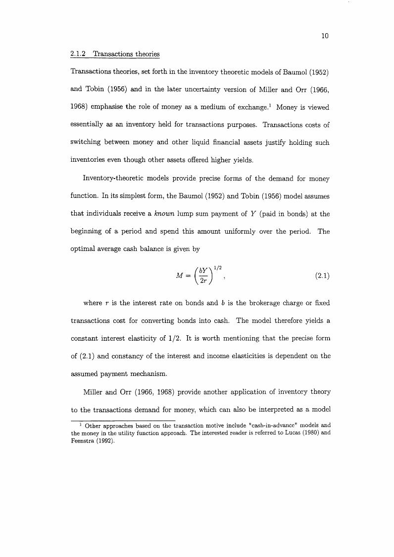
2 .1 .2 Transactions theories
Transactions theories, set forth in the inventory theoretic models of Baumol (1952)
and Tobin (1956) and in the later uncertainty version of Miller and Orr (1966,
1968) emphasise the role of money as a medium of exchange . 1 Money is viewed
essentially as an inventory held for transactions purposes. Transactions costs of
switching between money and other liquid financial assets justify holding such
inventories even though other assets offered higher yields.
Inventory-theoretic models provide precise forms of the demand for money
function. In its simplest form, the Baumol (1952) and Tobin (1956) model assumes
th a t individuals receive a known lump sum payment of Y (paid in bonds) at the
beginning of a period and spend this amount uniformly over the period. The
optimal average cash balance is given by
where r is the interest rate on bonds and b is the brokerage charge or fixed
transactions cost for converting bonds into cash. The model therefore yields a
constant interest elasticity of 1/2. It is worth mentioning th a t the precise form
of (2 .1 ) and constancy of the interest and income elasticities is dependent on the
assumed payment mechanism.
Miller and Orr (1966, 1968) provide another application of inventory theory
to the transactions demand for money, which can also be interpreted as a model
1 Other approaches based on the transaction motive include "cash-in-advance" models and the money in the utility function approach. The interested reader is referred to Lucas (1980) and Feenstra (1992).

11
of the precautionary motive for holding money since there is a minimum allowable
money holding below which a penalty must be paid. The key difference with the
In its simplest form, the model assumes th a t cash flows follow a random walk
w ithout drift in which, in a given time interval (say 1 /t of a day, where t is the
frequency of transactions), there is a probability of a positive or negative cash
(normalised to zero), the optimal policy consists of an upper bound, h, and a return
level, 2 . Whenever money balances reach the lower bound, 2 dollars of bonds are
converted into cash; whenever the upper bound is reached, h — z dollars of cash are
Thus, like the Baumol-Tobin model, the Miller-Orr model also yields a constant
is cr2, the income (or transactions) elasticity is ambiguous. I t is either 2/3 if one
considers the size of each cash flow, or 1/3 if one considers the rate of transactions.
Two features of these models can be used to explain the impact of financial
innovation on the demand for money. The first, common to both the certainty
and uncertainty approach, is the role of transactions costs in determining the de
Baumol-Tobin model is the assumption tha t cash flows are stochastic.
flow of m dollars (m is the amount the cash balance is expected to alter with a
probability of |) . Given a lower bound below which money balances cannot drop
converted into bounds. The optimal average cash balance (assuming a binomial
distribution for the net cash drain with a zero mean) is given by
(2 .2)
where cr2 is the daily variance of changes in cash balance (cr2 = m 2t).
interest rate elasticity, with a value of 1/3 instead of 1 / 2 . Since the scale variable

12
maud for money. Financial innovation, by lowering the converting other assets into
money, allows money holders to keep smaller money balances, meeting transactions
needs by more frequent transfers of funds from higher-yielding alternatives. The
second is the emphasis in the Miller-Orr version of the uncertainty of cash receipts
and disbursements as an important determinant of money demand. Greater vari
ance of cash flow leads to larger precautionary holdings of money holdings not to
be caught short. Innovations in cash management techniques are viewed as reduc
ing the variance of cash flow, thereby allowing firms to reduce their precautionary
balances (Judd and Scadding, 1982).2
2.1.3 Portfolio theories
Portfolio theories of money demand interpret the demand for money more broadly
as part of a problem of allocating wealth among a portfolio of assets which include
money. Money and other assets are viewed as alternative ways of holding wealth,
each yielding some mix of income and non-pecuniary service flows. In the case
of money, these services include the ease of making transactions as well as other
services with non-pecuniary yields such as liquidity and safety.
The individual wealth-holder in Tobin (1958) allocates her portfolio between
money and bonds. There is a trade-off between the net income receivable on bonds
and the risk associated with the total portfolio of bonds and money (perfectly liquid
with zero re tu rn ). For any given level of wealth it is possible to calculate the impact
of a change in interest rate on both the interest income and the capital gain or
2 For extensions of the Baumol-Tobin and Miller-Orr approaches the reader is referred to Barro and Fisher (1976) and Cuthbertson and Barlow (1991).

13
loss associated with the holding of different quantities of bonds and money. Under
the assumption of expected utility maximisation, the optimal portfolio mix can be
shown to depend on the individual’s degree of risk aversion and wealth, and the
mean-variance characteristics of the risky asset’s return distribution.
Tobin’s analysis implies a negative interest elasticity of money demand provid
ing another "rationalisation" of Keynes’s liquidity preference hypothesis (Judd and
Scadding, 1982). The approach has, however, two shortcomings. First, money does
not actually have a yield th a t is riskless in real terms. Second, in many economies
there exists a number of riskless assets paying a positive (or higher) rate of return
than money. Under such conditions the model implies th a t individuals would only
hold such assets and, therefore, tha t money is a "dominated asset" (Barro and
Fisher, 1976).
As in Tobin’s portfolio approach, Friedman (1956) offers a "restatement" of
the quantity theory which regards the primary role of money as a form of wealth.
According to Friedman, the demand for money can be analysed in the same way
as the demand for any asset. Money yields utility in the form of a flow of services
to the holder. Thus, the demand for money function contains a budget constraint
(either permanent income or wealth); the price of the commodity itself (money)
and its substitutes and complements (the rates of return on money and other assets
categorised into three types: bonds, equity, and goods); other variables determining
the utility attached to the services rendered by money relative to those provided
by other assets; tastes and preferences. Friedman expresses his formulation of the

14
demand for money as follows:
M dp j ( I p i ^ i Tb ^rri) T r m ^"e ^ 'm t 5 ( ^ ‘^ )
where M d/P is the demand for real money balances; Yp is a measure of wealth
known as permanent income (the present discounted value of all expected future
income); w is non-human wealth/wealth; r m is the rate of return on money, influ
enced by two factors: the services provided by banks on deposits (e.g. provision of
receipts in the form of cancelled checks, autom atic paying of bills) and the interest
payment on money balances; and r e are the expected rates of return on bonds
(abstracting from the possibility of capital gains and losses) and equity (abstract
ing from the effects of on equity prices of changes in interest rates and the rate
of inflation), respectively; 7re is the expected inflation rate, included as the rate
of return on real assets; u is a portm anteau symbol standing for other variables
affecting the utility attached to the services of money and also includes tastes and
preferences.
Tobin’s theory supports Keynes’s proposition tha t the demand for money is
sensitive to interest rates, suggesting tha t velocity is not constant and th a t nom
inal income might be affected by factors other than the quantity of money. In
contrast, Friedm an’s analysis implies th a t changes in interest rates should have lit
tle effect on the demand for money. Friedman argues that any rise in the expected
returns on other assets as a result of the rise in interest rates would be matched
by a rise in the expected return on money. He also suggests th a t random fluctu

15
ations in the demand for money are small and th a t the demand for money can
be predicted accurately by the money demand function. These views when com
bined mean th a t velocity is predictable—even though it is no longer assumed to be
constant—implying tha t a change in the quantity of money produces a predictable
change in aggregate spending as in the quantity theory of money.
2.1.4 Transactions with a shopping time constraint
Microeconomic transactions models attem pt to explain the holding of money for
transactions purposes within general equilibrium models. The most prominent
models of this kind axe proposed by McCallum (1989) and McCallum and Good-
friend (1992). These models analyse the demand for money in term s of the shop
ping time saved in carrying out transactions through the use of money (as opposed
to barter). Shopping time saved has value since it can be used to earn income or
to obtain utility from other uses.
The model in McCallum and Goodfriend (1992) has a representative household
maximising present and future utility for the consumption of goods and leisure
subject to the usual intertemporal budget constraint. Consumption goods can be
obtained in exchange for income only by shopping for them; the household faces a
shopping tim e constraint given by:
st = ip(ct,m t) (2.4)
The shopping time constraint is the amount of time required to carry out purchases
and is increasing in to tal transactions, c, but decreasing in the quantity of real
money balances carried on shopping trips, m. It follows th a t a decision to hold
16
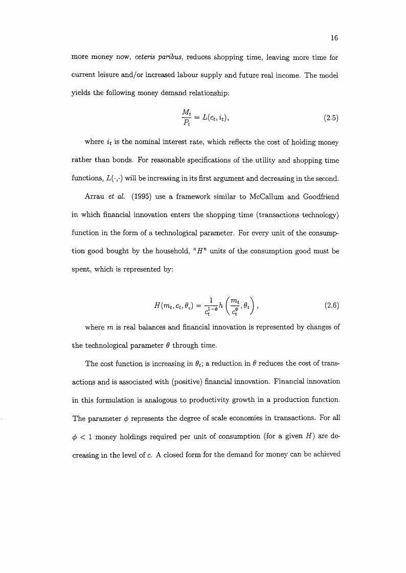
more money now, ceteris paribus, reduces shopping time, leaving more time for
current leisure and/or increased labour supply and future real income. The model
yields the following money demand relationship:
= £(<*,»,), (2.5)
where i t is the nominal interest rate, which reflects the cost of holding money
rather than bonds. For reasonable specifications of the utility and shopping time
functions, !/(-,■) will be increasing in its first argument and decreasing in the second.
Arrau et al. (1995) use a framework similar to McCallum and Goodfriend
in which financial innovation enters the shopping time (transactions technology)
function in the form of a technological parameter. For every unit of the consump
tion good bought by the household, " H " units of the consumption good must be
spent, which is represented by:
H {m u cu 9t) = - ^ h (2.6)ct \ c t /
where m is real balances and financial innovation is represented by changes of
the technological param eter 6 through time.
The cost function is increasing in 6t\ a reduction in 9 reduces the cost of trans
actions and is associated with (positive) financial innovation. Financial innovation
in this formulation is analogous to productivity growth in a production function.
The param eter <fi represents the degree of scale economies in transactions. For all
<p < 1 money holdings required per unit of consumption (for a given H) are de
creasing in the level of c. A closed form for the demand for money can be achieved

17
assuming h has the following form (omitting time subscripts):
a L c* ct .(2.7)
where K denotes a constant. This formulation yields the following money
demand function:
where -a is the semi-elasticity of the interest rate and 0 is the elasticity of
consumption. Equation (2.8) indicates tha t is the relevant measure of oppor
tunity cost. However, the most commonly used i can be justified by changing the
timing of the household problem. Furthermore, since this is a model of household
money demand the relevant scale variable is consumption; inclusion of firms and
government in the analysis would lead to the use of other scale variables.
There is a large body of empirical work on the demand for money. Initially, this
work was confined primarily to industrial countries, especially the United States
and the United Kingdom. More recently, there has been a renewed interest among
industrial and developing countries alike (see for example Siklos, 1993; Arrau et
al., 1995; Ericsson and Sharma, 1998; Dekle and Pradhan, 1999; Brissimis et al,
2003, Binner et al., 2004). One of the significant contributors of the recent boom
in empirical research on money demand is the m ajor advancements made in time
series econometrics from the late 1980s onwards, which have motivated researchers
to revisit the empirical models built previously (Sriram, 1999).
log(rot) = log(0 ,) + 4>log(c,j - a —7 - 7 (2 .8)
2.2 Econometric formulations
18
This discussion provides an historical background to the debate on the stability
of the demand for money starting from the mid-1970s, as well as a brief review
of the various models and procedures which have been used to estimate money
demand.
2.2.1 Historical development
Judd and Scadding (1982) noted that, prior to 1973, the evidence on the demand
for money was interpreted as showing tha t a stable money demand did exist.
This evidence has been extensively surveyed elsewhere (see for example Laidler,
1993). The substantial body of empirical research which had accumulated over the
postwar period sought to discriminate among the competing hypotheses suggested
by the different theories of the demand for money surveyed above. However, this
literature showed tha t it was not possible to distinguish empirically, with any
degree of precision, between competing hypotheses about the demand for money
(Judd and Scadding, 1982).
Most of the research up until the 1980s was carried out using partial adjust
ment models (PAMs) in which it is assumed th a t because of adjustment costs,
lagged money needs to be included in the money demand function for the desired
level of money holdings to m atch the actual level. Using the partial adjustment
framework, Goldfeld (1973) found evidence of a stable dem and function for US
narrow money (M l) over the period 1952:2-1973:4, which was positively related to
real GNP, negatively related to a representative short-term m arket rate (Treasury
bill or commercial paper rate) and the rate on savings deposits, and positively
19
related to lagged money. This specification became the conventional demand for
money function used by economists but was shown unable to explain a new set
of events which emerged in the United Kingdom and the United States in the
mid-1970s. The latter included changes in regulations concerning interest rate
ceilings on the deposits of commercial banks, innovations in short-term financial
markets associated with improvements in corporate cash-management techniques,
increases in the rate of inflation and interest rate compared with previous postwar
experience, and a greater emphasis on monetary targeting by the central bank.
In the UK, Haache (1974) showed th a t his money demand function was unable
to predict accurately outside of sample for the period after 1971, and recorded
significant negative forecasting errors for broad and narrow money. In the US,
Goldfeld (1976) came to the same conclusion showing th a t forecasts seriously over
predicted real money balances from 1974.3 Goldfeld labeled this phenomenon "the
case of the missing money". Other industrial countries experienced a similar prob
lem.
The systematic overprediction of real money balances (or underprediction of
velocity) by standard money demand functions stimulated an intense search for a
stable money demand function which dominated the research agenda of the next
twenty years or so. This search initially took two directions. The first direction
focused on whether an incorrect definition of money could explain why the demand
for money function had become unstable. For example, Garcia and Pak (1979),
3 The forecasts were out-of-sample dynamic simulations, which used actual interest rates and income but last period’s predicted money balances as the lagged dependent variable.

20
Wenninger and Sivesind (1979a, 19796), and Tinsley et al (1978, 1981) looked
for instrum ents th a t had been incorrectly left out of the definition of money used
in the US money demand function, most notably overnight repurchase agreements
(RPs ) . 4 These authors argued tha t for many large corporations, transactions costs
between money and RPs were so low tha t RPs were effectively money.
The second direction of search for a stable money demand function was to
look for new variables to include in the money demand function. Hamburger
(1977) specified the demand for real M l in the US as a function of real income,
lagged M l, and three rates of return-the commercial bank savings deposit rate, the
US government bond rate, and the dividend-price ratio (as a proxy for the rate of
return on equities and thus on physical capital) . 5 Although this specification was
found to be stable, its stability also depended on the assumption tha t the income
elasticity of the demand for money was unity, which led to strong criticisms (see
for example Hafer and Hein, 1979).
Heller and K han (1979) expanded the opportunity costs of money in their
money demand function to include the entire term structure of interest rates and
found th a t this produces a stable money demand function. However, Porter and
Mauskopf (1978), who re-estimated the Heller and Khan equation and dynamically
simulated it over 1973:3-1977:4, found tha t the cumulative prediction error by
1977:4 was on the same order of magnitude produced by the Goldfeld equation.
4 These are one-day loans with little default risk because they are structured to provide Treasury bills as collateral.
5 Including the dividend-price ratio in the list of interest rate arguments allowed for the possibility of substitution between money on the one hand and real capital and commodities on the other.

21
The problems associated with conventional money demand functions worsened
in the 1980s in the fane of a surprising slowdown in M l velocity in the US, which
conventional money demand functions could not predict. The relative stability
of M 2 velocity at the time suggested tha t money demand functions in which the
money supply was defined as M2 might perform substantially better than those
in which the money supply was defined as M l. For instance, Small and Porter
(1989) found th a t their M2 money demand function performed well in the 1980s,
with M2 velocity moving quite closely with the opportunity cost of holding M2,
which was defined as the market interest rate minus an average of the interest
paid on deposits and financial instruments th a t make up M2. However, in the
early 1990s, M2 growth underwent a dramatic slowdown, which traditional money
demand functions again could not explain.
A new strand of research identified a number of theoretical and econometric
problems associated with the partial adjustment framework. PAMs were shown to
suffer from specification problems and highly restrictive dynamics (see for example
Cooley and LeRoy, 1981; Goodfriend, 1985; Hendry, 1979). To counter these
problems, two major solutions were proposed—modifying the theoretical base and
improving the dynamic structure. The former led to BSMs (see for example Laidler,
1984; Cuthbertson and Taylor, 1987; Milbourne, 1988), and the latter to ECMs .6
ECMs have been used in a single equation context (see for example Mehra, 1993;
Hendry and Ericsson, 1991a, 19916; Baba et al., 1992; Hess et al., 1994; Janssen,
1996; Thomas, 1996) or in a vector error correction model (VECM) system context
6 Hendry et al. (1984) showed that PAMs and BSMs form special cases of ECMs.
22
(see B arr and Cuthbertson, 1991).
W hile BSMs ran into empirical difficulties. ECMs, because of their success,
rapidly became the primary tool to analyse the demand for money. Rose (1985)
obtained an ECM for US narrow money demand with constant parameters over
the 1970s, thus showing how Goldfeld’s episode of missing money of the mid-1970s
resulted from dynamic misspecification. However, Rose’s model broke down in the
1980s. Using a similar empirical model but accounting for financial innovations,
B aba et al. (1992) found a money demand function with a constant parameteri-
sation for 1960-1988. MacDonald and Taylor (1992) found a constant US money
demand function for annual data over 1874-1975. A similar chronology of ECMs
also exists for money demand in the UK. Relevant papers include Hendry and
Ericsson (1991a, 19916), Ericsson et al. (1994), and Ericsson et al. (1998).
2.2.2 Partial adjustment models
The partia l adjustm ent framework assumes th a t individuals constantly adjust their
current money holdings {Mt) to the desired long-run equilibrium (M*), which is
given and depends upon a vector of variables (e.g. interest rates, income) . 7 Agents
face the costs of being out of equilibrium, which can be explained in terms of in
terest income foregone or inability to purchase goods. Assuming the costs of being
above and below equilibrium are equal, these costs are represented by the quadratic
7 The adjustment of actual to desired money holdings can be in real terms as in the real partial adjustment models (RPAMs). with the lagged money variable in the form of M t_ i / P t-1 (where M are nominal money balances and P is the price level), or in nominal terms as in the nominal partial adjustment models (NPAMs), with lagged money in the form of M t~ i / P t ■ The reader is referred to Cuthbertson (1985, chapter 6 ) and Boughton (1992) for a discussion of the deficiencies (e.g. overshooting and implausible lags of adjustment) associated with both types of models.
23
term a(M t — M*)2, where a is the cost per unit of disequilibrium. Individuals also
face the costs of adjusting their portfolio of assets, which is also represented by
a quadratic term b(Mt — M t~i)2. Given M* and M t~ 1 an individual chooses M t
to minimise (one period) total costs which is the sum of the two quadratic terms.
The first order solution to this minimisation problem gives
= (2.9)
where 7 = jJj .
First, assuming tha t an increase in the demand for money is always met by
an increase in supply (as for example under a constant interest rate target by
the central bank) then the short-run desired demand derived in equation (2.9) is
equal to actual money balances and the money demand function can be estimated.
Second, assuming tha t the long-run desired demand for money Mt* has a linear
form and depends on current income Yt, and the expected return on alternative
assets R f, the long-run money demand function can be w ritten as
M l = m yYt — m rR l + ut (2-10)
where ut is an additive stochastic error fulfilling the usual stationarity condi
tions.
Substituting equation (2.10) in equation (2.9) and rearranging yields
Mt = b\Yt + + b^Mt-i + Vt, (2-11)
where b\ = 'yTny, 62 = —7 m r, and 63 = 1 — 7 are the estim ated coefficients and
v t = 7 Ut.

24
Equations such as (2 .1 1 ) have generally been estimated with ordinary least
squares (OLS) using the Cochrane-Orcutt technique to adjust for serial correlation.
In general, all estimates showed very low short-run elasticities for income (around
0.1) and interest rates (around —0.05), and a coefficient close to unity for the
lagged dependent variable. In contrast, the long-run interest elasticity was often
found to be much higher (around —0.3).
The partial adjustment framework has raised a number of criticisms, both on
theoretical (see for example Goodfriend, 1985) and empirical grounds. Econometric
problems include serial correlation, heteroskedasticity, simultaneity bias, model
misspecification, and spurious regressions due to the nonstationarity of the data
(Goodfriend, 1985; Yoshida, 1990).
2.2.3 Buffer stock models
There are a number of fairly distinct applied approaches to buffer stock money (see
for surveys Laidler, 1984; Milbourne, 1987; Mizen, 1994). The following discussion
gives a brief account of some general considerations underlying the idea of money
as a buffer stock drawing from Mizen (1997).
Buffer stock models have two common basic assumptions, which are an ex
ogenous money stock, tha t is, the money stock is primarily influenced by supply
factors, and a disequilibrium real balance effect. This is in contrast with PAMs,
which assume th a t the money stock is demand determined in the short run and
tha t the money market is in equilibrium with endogenous income, interest rates
and price level variables adjusting to clear the market. BSMs explain the demand

25
for money in the context of individual optimisation and the microeconomics of
adjustm ent in the market for money. Expectations are introduced into the analy
sis such th a t unexpected events in the present or expected events in the future
induce deviations from long-run equilibrium . 8 Since adjusting money balances is
costly, it can be optimal for an individual, when faced with a deviation of money
balances from long-run equilibrium, to allow th a t departure to persist in the short
run. Hence, BSMs reject the notion tha t all individuals hold their long-run level
of money balances at all times and tha t the money market in aggregate is contin
uously in equilibrium. Instead, BSMs adopt the view tha t tem porary departures
can be rational and optimal both at the individual and the market level.
C arr and Darby (1981), starting from the view th a t money is subject to ex
ogenous shocks, argue th a t money balances serve as a "shock absorber" or buffer
stock while money holders choose their new portfolios. They implement this idea
by starting with the real partial adjustment model and modifying it with "surprise
money", which allows money supply shocks and tem porary income to push real
money balances off the individual demand for money function in the short run.
The resulting functional form is an equation which allows for positive and negative
variations to individual money balances in response to unexpected events in the
short run. This equation is given by
m t = (1 - \ ) m t- i + Am* 4 - pt + by? + f ( m t - m “) + uu (2.12)
8 Buffer stock models based on the inventory principle (see, for example, Akerlof and Mil- bourne, 1980; Milbourne, 1987) are surveyed by Mizen (1994) and not reviewed here. These models have much in common with the Miller-Orr approach discussed above.

26
where (m t — m “) are unexpected nominal money supply shocks defined as ac
tual money supply, mt, minus anticipated money supply, m “; y j , is transitory
income defined as current minus permanent income and included since any un
expected variations to income are temporarily held as money ;9 m* are long-run
desired money holdings described as a function of permanent income and interest
rates; A, b, and / are coefficients derived from the param eters of the model, and
Ut is the white noise error term. Carr and Darby recognise tha t ut is correlated
w ith (m t — ntf) and OLS estimation yields inconsistent estimates of the parame
ters. Hence, they use an instrum ental variables procedure, namely two-stage least
squares (2 SLS).
Although Carr and Darby did not examine the issue of the missing money
episode, one can see from equation (2.9) tha t in periods of relative "calm" the
partial adjustm ent model would be expected to perform reasonably well, but when
the expectational errors become more im portant in more "turbulent" times (when
the coefficients / and b are significantly different from zero), they would be the
cause of serious forecast errors as observed in the mid-1970s. However, both the
estim ation procedure of Carr-Darby and their conclusions have been extensively
criticised (Cuthbertson and Taylor, 1986; MacKinnon and Milbourne, 1988).
Cuthbertson and Taylor (1987) propose a model in which departures from
current period equilibrium result not just from unexpected events but from an
ticipated events ahead of the current time period, such as expectations of future
9 Carr and Darby (1981) argue that permanent income is the appropriate concept for the long-run demand for money and that transitory income will temporarily be kept as money until adjustment can occur.

27
monetary policy. The individual faces the cost of being out of equilibrium and the
cost of adjusting balances in the future as well as the present. Money holdings
axe composed of planned components based on the minimisation of an intertempo
ral cost function and unplanned components resulting from unanticipated shocks.
This approach assumes multi-period quadratic costs of adjustment. The resulting
money demand function is given by
OO
TTLt = Xrrit-i + (1 — A)(1 — A-P)^ ^( X D y -f- tr ̂ -f- e ,̂ (2.13)i = i
where A is a parameter of the model, are unexpected shocks to money
holdings, D is a known discount factor, m* are long-run money balances, and et is
the white noise error term.
Milbourne (1987, 1988) summarises the various theoretical and empirical crit
icisms raised by the buffer-stock approach. These criticisms help explain why
"subsequent work favours the ECM interpretation" (Cuthbertson, 1997).
2.2.4 Error correction models
The im portant feature of the error correction model is th a t it provides significant
emphasis on the time series characteristics of the da ta and the underlying data
generating process. Unlike the PAM and BSM, which severely restrict the lag
structure by imposing implausible lags of adjustment or relying solely on economic
theory, the ECM allows economic theory to define the long-run equilibrium while
the short-term dynamics is determined from the data. The following discussion on
ECMs draws from Alogoskoufis and Smith (1991).

28
The current popularity of ECMs is largely due to David Hendry, whose work
was influenced by Phillips (1954, 1957) and Sargan (1964). One of the most in
fluential of Hendry’s contributions on error correction models is Davidson et al.
(1978), in which the ECM form for the relationship between consumers expendi
tu re and income is introduced . 10 In Hendry’s work (see for example Hendry et
al., 1984), the best known representation of the ECM in a simple money demand
model w ith three variables, m — p (real money) y (income) and R (interest rate)
is a log-linear equation of the form
A (m - p)t = a + /3XA yt + f32A R t - 7 ((m - p)t_1 - - R ^ ) + et (2.14)
where et is a white noise error term.
The static long-run solution of this equation (when (m — p)t = (m — p)t-i =
m - p , yt = yt-1 = y and Rt = Rt- 1 = R) is
(m - p) = 0 / 7 + y + R (2-15)
Since most economic time-series are highly trended with stationary growth
rates, th a t is, they are integrated of order one, 1(1), the two sides of equation
(2.14) are of different orders of integration, with A (m — p)t stationary (integrated
of order zero) and ( m — p)t-i, Vt- 1 and Rt~ 1 all 1(1), unless the linear combination
(m — p)t~ 1 — yt-1 — Rt- 1 is also stationary. In general, linear combinations of
1(1) variables are also 7(1), but if they are 1(0), then the variables are said to be
cointegrated.
10 Although the estimated relationship is given a "feedback" interpretation, the term "error correction" is not used in the paper. The term is first introduced in Hendry (1980).

29
Engle and Granger (1987) proposed a very popular procedure for testing coin
tegration, in which residuals from a static regression of integrated variables are
tested for having a unit root. The static regression is interpreted as a cointegrat-
ing relation if the hypothesis of a unit root in the residuals is rejected, where tests
for a unit root are typically based on the augmented Dickey-Fuller (1981) statistic.
Engle and Granger show that if the variables are cointegrated then there exists
an error correction representation. Conversely, if there is an error correction rep
resentation for the series, then they are cointegrated . 11 While intuitive and easy
to implement, the Engle-Granger procedure often has little power to detect coin
tegration, and the long-run coefficient estimates from the static regression can be
badly biased in finite samples (see Banerjee et al, 1986, and Kremers et al., 1992).
Johansen (1988, 1995) developed an asymptotically fully efficient, maximum
likelihood systems estimation procedure for determining the number of cointegrat-
ing vectors and for estimating and conducting inference about the cointegrating
vectors. The procedure is based on the so-called reduced rank regression method
and presents some advantages over the Engle and Granger two-step approach (see
Johansen and Juselius (1990) for money demand applications). First, it relaxes
the assumption th a t the cointegrating vector is unique, and second, it takes into
11 Engle and Granger define a vector stochastic process xt, which is / ( l ) , as having an error correction representation if it can be expressed as
j4(Zr)(l - L)xt = - y e t - i + et
L is the lag operator, such that (1 - L)xt = x t — x t - i - A(L) is a polynomial in L of the form (cuo + a i L + 0 2 -5 2 + ...)• Et is a stationary multivariate disturbance. It is assumed that j4(0) = I, A{ 1) has all elements finite and 7 ^ 0. The cointegrating vector is a, where et = a 'x t = 0, thus et is interpreted as a measure of the error or deviation from equilibrium. In other words, if the variables are cointegrated, the residuals can be treated as the equilibrium correction term in subsequent specification of a dynamic model for the variables involved.

30
account the short-run dynamics of the system when estimating the cointegrating
vectors.
The test of the number of cointegrating vectors (r) can be conducted using
either of two statistics: the trace statistic, which tests the null hypothesis tha t
the number of cointegrating vectors is less than or equal to r against a general
alternative, or the maximum eigenvalue statistic, which tests a null of r cointe
grating vectors against a specific alternative of r + 1 . Asymptotic critical values
for testing the number of cointegrating vectors appear in Osterwald-Lenum (1992)
inter alia.12
12 Dolado et al. (2001, p. 643) gives the following example to illustrate the underlying intuition behind Johansen’s testing procedure. Assume yt represents a vector of n / ( l ) variables and has a vector autoregressive representation of order 1 (VAR(l)) such that A ( L )y t = e t with A(L) = I n — A \ L (note that Johansen deals with the more general case where y t follows a VAR(p) process). This process can be reparameterised in the vector error correction model (VECM) representation as
Ayt = Dyt- i + etwhere D = (A l — /„) = —A (l) = — BT, and e t is white noise. To estimate B and T, D is
estimated using maximum likelihood estimation, subject to some identification restrictions since otherwise B and T could not be separately identified. If rank(D) = 0, then y t is 1(1) and there are no cointegrating relationships (r = 0 ), whereas if rank(D) = n, there are n cointegrating relationships among the n series and hence y t is 7(0). Thus testing the null hypothesis that there are r cointegrating vectors is equivalent to testing whether rank(D) = r.
31
2.3 Financial liberalisation, stationarity and structural stability of MDFs
Model stability is necessary for prediction and econometric inference. Since a
param etric econometric model is completely described by its parameters, model
stability is equivalent to parameter stability (Hansen, 1992). While model insta
bility makes it difficult to interpret regression results, it is of particular importance
in policy analysis to know if econometric models are invariant to possible policy in
terventions. A necessary condition for making a conditional money demand model
immune from the Lucas (1976) critique is within sample param eter constancy (Er
icsson, 1998).
Model instability may be caused by regime shifts/structural breaks or by the
omission of an im portant variable . 13 Both regime shifts and a missing variable in
the money demand function have been linked to financial liberalisation and widely
blamed for the instability of empirical money demand models (Hendry, 1979).
A broad definition of financial liberalisation involves institutional and policy
changes as well as technological progress in transactions, which one usually in
terprets as financial innovation. Abiad and Mody (2005) identify three sources
of financial liberalisation. First, reforms may be triggered by discrete events, or
shocks, th a t change the balance of decision making such as various types of crisis,
and external influences such as the leverage exercised by international financial
institutions. Second, learning may foster reforms by revealing information tha t
13 Regime shifts/structural breaks are structural changes in a time series sample. Although the exact definition of structural changes has not been given in the literature, it is usually interpreted as changes of regression parameters (Maddala and Kim, 1998).

32
causes reassessment of the costs and benefits of the policy regime. Third, reforms
may be conditioned by political ideology of the ruling government and structural
features such as openness to trade, legal system and form of government.
These sources of changes have different implications for the timing of liberalisa
tion. Shocks leads to immediate policy change while learning allows for sustained
changes. Existing measures of liberalisation can refer to a one-time change in rules
(i.e. episodes of liberalisation), or to continuous proxies such as the level of finan
cial development in an economy. Liberalisation is therefore "a mix of the episodic
and the ongoing" (Abiad and Mody, 2005). While the timing, direction and size
of policy changes may vary, it is important to observe th a t financial liberalisation
is most likely to have permanent effects on the demand for money. Empirically,
this phenomenon can be identified with all permanent shifts in money demand un
related to the behaviour of the explanatory variables th a t appear most commonly
in the literature.
2.3.1 Financial liberalisation and the random walk hypothesis
From the univariate point of view, structural breaks in nonstationary series can be
viewed as permanent large shifts occurring intermittently, as against permanent
small shifts occurring frequently and generating / ( l ) effects. The two forms of
nonstationarity due to unit roots and regime shifts are closely related (Rappoport
and Reichelin, 1989), and can be hard to discriminate empirically (Perron, 1989;
Hendry and Neale, 1991). Stochastic process w ith short memory or stationarity
th a t exhibit structural changes can display similar characteristics as the ones ob-

33
served in long memory or long range dependent processes. W hen one observes
stationary series with structural breaks, the few occasional events or shocks with
long-duration effects would produce certain persistence or symptoms of nonsta
tionarity (Jimeno et al, 2006).
The distinction between random walk or broken trend stationarity of the se
ries in the money demand function is im portant. Perron (1989) argues that, if a
series is stationary around a deterministic trend th a t has undergone a permanent
shift sometimes during the period of consideration, failure to take account of this
change in the slope will be mistaken by the standard unit root test as a persistent
innovation to a stochastic (nonstationary) trend. Hence a unit root test tha t does
not take account of the break in the series will have very low power. 14 If one
assumes th a t the breakdate of the trend function is exogenous and chosen inde
pendently of the data, the unit root test can be adjusted by including composite
dummy variables to ensure there are as many deterministic regressors as there are
deterministic components in the data generating process. 15 Tests tha t are valid
in the presence of such a break at a known point in time have been developed by
Perron (1989; 1990) and Perron and Vogelsang (1993a; 19926).
However, it is unlikely tha t the exact breakdate will be known a priori. Fur
thermore, as argued by Christiano (1992) inter alia, tests th a t trea t the breakdate
as exogenous are not appropriate in circumstances where the date of the break is
14 There is a similar loss of power if there has been a change in the intercept, possibly in conjunction with a shift in the slope of the deterministic trend.
15 These dummy variables take a value of (0, 1) to allow for shifts in the intercept or are multiplied by a time trend to take into account any change in the slope of the deterministic trend.
34
selected by reference to the data, for instance by looking at the plots of the series.
Thus, one should use tests that endogenise the breakdate. Such tests have been
proposed by Banerjee et al. (1992), Zivot and Andrews (1992), Perron (1997),
Perron and Vogelsang (1992a) and Vogelsang and Perron (1998) inter alia.
From the multivariate point of view, conventional cointegration tests could
yield misleading results in the presence of structural breaks (Leybourne and New-
bold, 2003). Gregory et al (1996) study the sensitivity of the augmented Dickey-
Fuller (ADF) test for cointegration in the presence of a single break. Their Monte
Carlo results show th a t the rejection frequency of the ADF test decreases substan
tially. Thus, in the presence of a break, one tends to underreject the null of no
cointegration. The underrejection is similar to the underrejection of the unit root
null hypothesis in the univariate case. However, in this case, the underrejection of
the null indicates correctly tha t the constant param eter cointegrated relationship
is not appropriate.
In a similar development to the extension of unit root test by deterministic
components, cointegration tests have also been augmented by dummy variables,
and made robust again structural breaks. Gregory and Hansen (1996) propose
to test the null of no cointegration against the alternative of cointegration in the
presence of a regime shift. The shift considered is a single break of unknown timing
in the intercept and /o r slope coefficients in the cointegrated relationship.

35
2.3.2 Financial liberalisation and the missing variable hypothesis
It is difficult to distinguish between genuine structural breaks th a t even a correctly
specified money demand function using appropriate modelling methodology would
break down under, and an omitted variable, which would also induce parameter
instability when a misspecified regression based on an inappropriate modelling
strategy is used.
To illustrate this point consider the theoretical money demand function of Ar
rau et a l (1995) (equation (2.8)), which has the following econometric specification
(in log-linear form)
m t = r)t + /3'xf + vt (2.16)
where m t is money, x* = [2/4, Rt]', yt is the scale variable, R t is the vector of
variables measuring the opportunity cost of money, rjt = log(0 ), 6 is financial
liberalisation, and vt is a stationary error term.
If the param eter capturing financial liberalisation in equation (2.16), rjt , was
a stationary variable, the money demand function could be estim ated without
controlling for financial liberalisation, since the process of liberalisation would be
part of a stationary error term. However, in so far as financial liberalisation has
permanent effects on the demand for money, equation (2.16) w ith an intercept
instead of r}t would be misspecified and cointegration of the money demand function
would not be obtained. Absence of cointegration would indicate th a t while the scale
and opportunity cost variables may be necessary for "pinning down" the steady-

state dem and for money, these axe not sufficient (Arrau et al, 1995). Intuitively,
when compared to the previous hypothesis, this view of financial liberalisation
suggests th a t the latter, while also having large permanent effects on the demand
for money, is best characterised as an ongoing process of structural change rather
th a t one inducing episodic regime shifts.

CHAPTER 3
AN OVERVIEW OF FINANCIAL LIBERALISATION IN INDONESIA
In the early 1980s, Indonesia was a high growth, low-income country heavily
dependent on oil, with a financial system th a t was typical of most developing
countries (Booth, 1998). The fall in oil revenues in 1982 prom pted the Indonesian
government to reform the financial system to make it more effective at mobilising
and allocating savings to m aintain investment. Financial reforms in Indonesia were
implemented through major policy packages, most notably in 1983, 1988, 1990
and 1991. Financial liberalisation included the lifting of interest rate controls,
the removal of directed credit programmes, the deregulation of banking activities
and the opening of the capital market to foreign investors. The process, however,
suffered a few set backs, most notably in 1997 when the country was hit by a severe
economic crisis.
Although unique, the Indonesian experience is far from isolated. In fact, in
the last quarter of the twentieth century, financial sector liberalisation was high on
the agenda of policymakers and the trend worldwide was towards more liberalised
financial systems. In two seminal papers, McKinnon (1973) and Shaw (1973) argue
th a t financial repression is an obstacle to economic growth. Financial sectors,
once they have been liberalised, can provide financial resources as cheaply and
efficiently as possible which in turn stimulates the growth of the real economy.
The experiences of financial liberalisation in Indonesia and elsewhere, however,
38
have also raised concerns about the possible link between financial liberalisation
and economic crises . 1
The purpose of this chapter is to provide an overview of the financial reforms
carried out in Indonesia since 1983 and discuss significant changes in monetary
policy instrum ents and direction implemented in parallel with these reforms.
3.1 Banking system reforms
Throughout the 1970s, the Indonesian banking system exhibited many of the
characteristics of financial repression described by McKinnon and Shaw. As de
scribed by McLeod (1999a, pp. 259-60)
the banking sector was dominated by five State commercial banks...
Regulations effectively prohibited the establishment of new private sec
tor banks (domestic and foreign-owned), and heavily constrained the
expansion of existing branch networks... State-owned banks accounted
for roughly 80 per cent of to tal commercial bank assets throughout this
period.
State-own enterprises (SOEs) were required to hold their deposit accounts at
the State banks and were also the main borrowers of S tate banks’ loans. Both
S tate and private banks did not compete for deposits because their lending was
limited by credit ceilings. Under the directed subsidised credit schemes, known
as liquidity credit schemes, State banks provided loans to targeted borrowers at
1 The reader is referred to Levine (1997) for a review of the literature on financial liberalisation and economic growth and Demirguc-Kunt and Detragiache (2001) for a discussion of the causality from financial liberalisation to economic crises.

39
relatively low interest rates, with the loans eligible for refinancing from the central
bank a t subsidised rates . 2 State banks had, therefore, little incentive to improve
the level of service to borrowers and depositors alike, to offer attractive interest
rates, or to improve their loan appraisal skills and their capacity to minimise loan
losses (McLeod, 1999a).
By the early 1980s, the credit policies had led to a repressed financial system,
w ith subsidised credit largely benefiting the State entreprises, which could access
low-cost liquidity through their links to the State banks. In 1982, the central bank
dominated the financial system, with about 45 percent of gross banking assets (22
percent of GDP). Deposit mobilisation was limited by the credit ceilings, limits
on State banks lending and deposit interest rates, and branching. Prom 1975 to
1981, financial depth, as measured by the ratio of broad money, or M2, to nominal
GDP, stagnated at about 16 percent, with an usually high fraction (60 percent) of
M l (currency and demand deposits) in broad money. The one-year deposit rate at
the State banks, in real terms, averaged —2.5 percent from 1975 to 1982 and —4.8
percent from 1979 to 1982 (Hanna, 1994).
The fall in oil revenues in 1982, which led to a deterioration in Indonesia’s
current account deficit and a fall in GDP growth, prom pted the Indonesian gov
ernment to reform the financial system.
2 According to Hanna (1994, p. 5), direct credit allocation accounted for 48 percent of all bank lending by 1982. State banks granted loans at rates of 6 to 12 percent while the rediscount rates varied from one-third to one half of the subsidised rate paid by the borrower. The portion of a loan eligible for refinancing typically varied from 20 to 100 percent.

40
3.1.1 The June 1983 reforms
In June 1983 the government introduced a reform package known as PAKJUN,
a m ajor aspect of which was the curtailment of the subsidised loan programmes.
The evidence had shown that the experience with the directed credit schemes did
not have much impact on the course of structural change of the economy (Patten
and Rosengard, 1991). Lending rates were freed and controls on all time deposit
interest rates were removed to force the State banks to continue to lend based on
deposit inflows alone . 3 By the end of 1983, most subsidised loan programmes had
been discontinued.
State banks responded to these policies by moving their time deposit and
lending rates up to levels slightly below the prevailing rates at the private banks.
Bank deposits increased very rapidly, with the growth of time deposits, those of
the State banks in particular, far exceeding th a t of demand deposits. In contrast,
the growth of bank lending was much more rapid in the private banks than in the
S tate banks. As a result most State banks found themselves with an excess of funds
which they were unable to lend, and became "chronic lenders" to the interbank
market, while many private banks became "chronic borrowers" (Binhadi and Meek,
1992).
Although the reforms increased the flexibility of existing banks in pricing and
allocating credit, they did not lower entry barriers, either among banks or between
banks and other financial institutions . No new foreign banks were allowed entry,
3 Private banks had not been subject to the interest rate controls, but had been under the credit ceilings.

41
and the opening of new branches continued to be severely constrained, giving State
banks a clear advantage (Hanna, 1994).
3.1.2 The October 1988 reforms and further refinements
The government introduced in October 1988 a further deregulation package known
as PAKTO (Government of Indonesia, 1988). The reforms contained in PAKTO
removed impediments to competition by opening up possibilities for establishing
new banks and new branch offices of existing banks (Binhadi, 1995). New domestic
banks could be established, subject only to a small minimum capital requirement.
Foreign banks were allowed to set up joint ventures w ith existing domestic banking
partners .4 In addition, State enterprises were perm itted to place up to half of their
deposit funds with private banks. Another aspect of PAKTO was the reduction of
the required reserve ratios from a multiple set of nominal rates tha t averaged about
1 1 percent for all banks together to a uniform level of 2 percent of all third party
liabilities, thereby reducing the intermediation costs for banks and increasing the
potential monetary expansion from any given increase in reserve money (Cole and
Slade, 1996). Further refinements of the new rules came into supplementary pack
ages introduced in March 1989 (Government of Indonesia, 1989) and January 1990
(Government of Indonesia, 1990), with the last significant (pre-crisis) deregulation
reform contained in the banking law introduced in February 1992.
The March 1989 reform package known as PAKMAR removed controls on
4 Domestic banks were permitted to open new branches wherever they wanted, without limit, although foreign and foreign joint-venture banks were still only permitted no more than six offices each in only six major cities (McLeod, 1999a).

42
banks’ offshore borrowing and introduced a prudential limit on banks’ net open
positions (NOP) . 5 The package announced on January 1990 known as PAKJAN
abolished the remaining subsidised loan programmes, and moved interest rates
on refinance from the central bank closer to market levels (Chant and Pangestu,
1994). The reform contained in the banking law enacted in February 1992 allowed
foreign entities to acquire shares in domestic banks listed on the stock exchanges,
and permitted the State banks to be listed (McLeod, 1992).6
60 -
1980 1982 1984 1986 1988 1990 1992 1994 1996 1998 2000
Deposit rate Inflation Lending rate
Figure 3.1: Interest and inflation rates, 1980-2000
5 This term refers to the gap between banks’ liabilities and assets denominated in foreign currencies, relative to their capital. Under the NOP constraint, banks may bring in as much foreign funds as they like provided they on-lend them predominantly in the same currencies.
6 Foreign shareholding, however, was not permitted to exceed 49 percent of the total, and the government was required to majority shareholding in any state bank whose shares were offered to the public.

43
3.1.3 The February 1991 and May 1993 reforms
In 1990, the private sector Bank Duta verged on bankruptcy as a result of its
involvement in large-scale currency speculation (for a discussion, see Soesastro
and Drysdale, 1990). Bank D uta had acquired a very large NOP, and subse
quent exchange rate changes caused it to loose about US$420 million (McLeod,
1999a). This episode prompted the government to introduce in February 1991 a
package of new prudential regulations known as PAKFEB (Government of Indone
sia, 1991). The new prudential measures imposed various ratios for evaluating
bank soundness and restricted bank activity in connection with the capital market
(Hendrobudiyanto, 1994; Habir, 1994). The most im portant measures included
new risk-adjusted capital adequacy requirements (CARs) (in line with the Basel
Agreement), new loan/deposit ratio standards, and new restrictions on foreign ex
change NOP for authorised foreign exchange banks. Further measures were also
taken in 1992 including new laws on banking, insurance, and pensions.
In May 1993, a reform package known as PAKMEI relaxed and adjusted some
of the PAKFEB bank prudential restraints in order to encourage new lending.
Among other things, the CAR was marginally eased, the risk weighting of unused
credit lines and loans to government enterprises was reduced from 100 percent to 50
percent, and capital as well as deposits was counted in calculating the loan/deposit
ratio.
A number of previous deregulation measures were also reversed. BI reimposed
controls on foreign borrowings by banks in 1991 (Muir, 1991).7 In the mid-1990s,
7 Bank Indonesia Directors Decree No. 24/52/KEP/DIR. dated 29 November 1991.
44
BI adopted a target for the rate of growth of bank lending. The central bank also
closed entry to almost all of the non-bank financial sector, which comprises leasing,
factoring and consumer finance companies (with the exception of insurance and
pension funds) in December 1995. Regulations on the issuing of commercial papers
were also imposed in 1995.8 Under these regulations, any commercial paper issued
or traded by banks had to be rated "investment grade" by a domestic agency
established by the government (PT Pefindo) and was limited to a maximum 270
days’ maturity.
3.1.4 Im pact of the reforms on the banking system
The liberalisation of interest rates, together with the substantial progress achieved
in reducing inflation, resulted in positive real interest rates during the 1980s and
m ost of the 1990s (Figure 3.1 ) . 9 By contrast, prior to 1983, real interest rates had
tended to be negative. The immediate impact of liberalisation was to move rates
upwards.
Positive real interest rates in the 1980s contributed to financial deepening (or
m onetisation). For the period 1983-1988, the ratio of M2 to GDP increased from
17 to 30 percent in 1988 and further to about 60 percent at the end of 1997 (Figure
3.2). In contrast, the ratio of M l to GDP fluctuated within a range of 8 - 1 2 percent
over the same period.
During this period to tal assets of commercial banks increased 10-fold to Rp715.2
8 Bank Indonesia Directors’ Decree No. 28/52/KEP/DIR, dated 11 August 1995.9 The real interest rate can be measured by the nominal interest rate minus the change in
the consumer price index in the last 12 months. This assumes that inflation expectations can be approximated by actual inflation over the past 12 months.

45
trillion, exceeding for the first time the size of the country’s GDP; nonbank finan
cial institutions (NBFIs) also flourished with total assets growing at an annual
compound rate of 56 percent in 1991-1996, reaching Rp80 trillion by end-1996
(Chou, 1999, p. 36). The banking system, nevertheless, still held about 65 percent
of the financial sector’s total assets in 1997.
50 -
1983 1985 1987 1989 1991 1993 1995 1997 1999
Currency M1 M2
Figure 3.2: Monetary ratios as percentage of GDP, 1983-2000
Changes in the ratios of time and savings deposits to GDP and demand de
posits to GDP (Figure 3.3) also offer a good perspective on the growth of the
banking system. Time and savings deposits, having been stagnant relative to out
put prior to 1983, suddenly began to increase rapidly. The impact of liberalisation
on demand deposits, however, is less clear cut.
The 1988 reforms also stimulated the physical expansion of the banking indus
try. Some ninety-four new private domestic banks were established in the period

46
Outstanding Balances as % of Nominal GDP
50 -
40 -
10 -
1980 1982 1984 1986 1988 1990 1992 1994 1996 1998 2000
d e m a n d tim e & savings
Figure 3.3: Impact of deregulation on bank deposits (outstanding balances as %
of nominal GDP), 1980-2000
up to June 1997, plus thirty-two joint foreign ventures; some 3,674 new branches
were added to the private banks’ network, while only 611 new State bank branches
appeared; the total number of branches increased from 1,728 to 6,337 during this
period (McLeod, 1999a, p. 275).
By opening up the financial sector to new entrants, most of which were small
and joint venture banks, the reforms intensified the competition for funds. In 1983-
1988, the seven State banks’ share of total outstanding credit averaged around 65
percent. In contrast, after three years of liberalisation their share dropped to 56
percent in 1991 and further to 40 percent by end-1997. Private banks experienced
an annual growth rate in their assets and credits of 60 and 39.5 percent in the four
years after PAKTO, compared with 2 2 and 2 1 percent for the State banks (Chou,
1999, p. 36).
47
3.2 Capital market reforms
The capital market includes both equity and bond markets. The equity mar
ket in Indonesia is made of three Stock Exchanges: the Jakarta Stock Exchange
(JSX), the Surabaya Stock Exchange (SSX), and an over-the-counter (OTC) m ar
ket known as Bursa Paralel (created in 1988 and merged with the SSX in 1994).10
While the bond market expanded rapidly between 1992 and 1997, it remains small
and bank finance is still the dominant form of nonequity capital (Wells, 1999).11
Originally opened in 1912 under the Dutch colonial government, the JSX re
opened on 10 August 1977 with only one company listed. A year before, the Capital
Market Executive Agency (Badan Pelaksana Pasar Modal, or BAPEPAM), an
agency which answers to the Ministry of Finance, had been established as capital
market regulator. In 1978, the Ministry of Finance issued decrees authorising the
establishment of trustees and guarantors in the capital m arket . 12 The following
year, the government opened up the right for all Indonesian financial institutions,
including pension funds, to buy securities on the Stock Exchange . 13 In 1981, a
further decree was announced allowing continuous trading at the Stock Exchange . 14
10 The SSX (and Bursa Paralel) established in 1989 is facilitating three markets: stock trading for small and medium scale companies, bond trading/reporting for corporate and government bonds, and derivatives trading for stock index futures.
11 The bond market is, therefore, omitted from this discussion. The interested reader is referred to Wells (1999).
12 Ministry of Finance Decrees No. 458/KMK.011/1980 and No. 459/KMK.011/1980.13 Ministry of Finance Decree No. 313/KMK.011/1979.14 Ministry of Finance Decree No. 161/KMK.011/1981.
48
3.2.1 The December 1987 and December 1988 reforms
On 23 December 1987, the Ministry of Finance issued a package of deregulation
measures aimed at the capital market known as PAKDES I. The measures soft
ened requirements for licensing underwriters, brokers, dealers, trustees, and guar
antors; outlined requirements and procedures for public offerings of both shares
and bonds, requirements for the prospectus, financial statem ents, and reporting
and public recording of these documents. PAKDES I also authorised foreign port
folio investment in the JSX. Foreign investors were allowed to purchase shares
up to an am ount allowed by the provisions of the Investment Coordination Board
(.Badan Koordinasi Penanaman Modal, or BKPM) on foreign capital participation.
Finally, the package also eliminated the limitations on daily price movements on
the JSX, thereby freeing it from direct price controls (Cole and Slade, 1996).
A second package, known as PAKDES II, was issued in December 1988. The
package focused on stimulating the capital market as well as non-bank financial
institutions (NBFIs) and the insurance sector. 15 The capital market measures in
cluded provisions authorising the establishment of a private securities exchange
in Indonesia, including prohibitions against insider trading. New regulations also
opened the m arket to foreign investors by allowing up to 85 percent foreign share
ownership in securities companies. Another im portant measure was to subject do
mestic deposits to a 15 percent withholding tax, the same tax levied on dividend
15 NBFIs are categorised into two: those engaged primarily in capital market activities and the rest. The former are regulated and supervised by BAPEPAM, while the rest-finance companies, venture capital companies, insurance companies, and pension funds-are supervised by the Ministry of Finance, with assistance from BI in some cases (Chou, 1999).
49
payments. The aim was to move towards a more level playing field for financial in
strum ents. PAKDES II also contained new regulations covering the establishment
of multi-finance companies allowed to engage in leasing, factoring, venture capi
tal, credit card operations and consumer credit. The same activities were made
available to banks (Hanna, 1994).
3.2.2 The December 1990 reforms and 1992 Amendments to the Income Tax Law
A third package, known as PAKDES III, was adopted in December 1990. The pack
age provided for the privatisation of the JSX (under the ownership of P T Jakarta
Stock Exchange), which took place on 13 July 1992. The package also provided for
the conversion of the Capital Market Executive Agency into the Capital Market
Supervisory Agency (under the same acronym, BAPEPAM). New requirements for
securities companies (including brokers and underwriters) were also adopted: the
company listing requirement, the requirement for cash dividends, and the delisting
criteria. The first ruling meant tha t all shares had to be traded on an exchange
when they were sold, and th a t a larger percentage had to be available to foreigners;
the second ruling was th a t a company could be delisted if it did not pay a cash
dividend for three consecutive years; the third ruling was th a t a company could
be delisted on the basis of one or more of the following criteria: less than 1 0 0
shareholders, no trades for six consecutive months, no cash dividend and/or losses
of 50 percent for three consecutive years, and equity less than Rp3 billion (Cole
and Slade, 1996).
The 1992 Amendments to the Income Tax Law set out the principles to re

50
solve outstanding tax issues affecting the development of the capital market. The
existing Income Tax Law of 1984 contained three discriminatory taxes: a tax dis
crim ination between interest income from securities and from bank deposits, the
triple taxation of investment funds and the discriminatory taxation of dividends of
subsidiaries of banks and other financial institutions. The amendments introduced
in 1992 imposed full taxation on the interest on corporate time deposits, allowed
tax exemption on the income from investment funds distributed to unitholders,
and perm itted dividends from subsidiaries of financial institutions to receive the
same treatm ent as all other dividends.
3.2.3 Corporate and capital market laws
The Corporate Law of 1995 governs the establishment and operation of limited lia
bility companies in Indonesia. The law provides a number of rights to or protection
of shareholders including access to regular and reliable information free of charge,
one share one vote, mandatory shareholders’ approval of interested transactions,
m andatory shareholders’ approval of major transactions, mandatory disclosure of
connected interests, independence of auditing, mandatory independent board com
m ittee, and severe penalties for insider trading.
The Capital Market Law of 1995 regulates companies listed in the stock ex
change, delineating the tasks and responsibilities of the Capital Market Supervisory
Agency. It regulates the requirements of investment companies, securities compa
nies, underwriters, brokers, investment managers, investment advisors, and other
supporting agencies. It also regulates reporting and auditing procedures, trans
51
parency requirements, insider trading investigation, and administrative and legal
punishment.
3.2.4 Impact of the reforms on the capital market
The capital market has grown significantly following the three deregulation pack
ages introduced in the late 1980s. The number of equity share-issuers at the JSX,
132 in 1990 rose to reach 379 at the end of 2001 and the value of equity issues
outstanding went from just over Rp8 trillion to almost Rp71 trillion during this
period (Table 3.1).
The role of foreign capital has been crucial in driving the market in the early
part of the 1990s. Foreign investors have dominated the m arket up until the end
of 1997 according to the percentage of shares they owned at the end of each year
(Table 3.2).
The increasing im portance of the capital market as a source of funds for busi
nesses and as an investment alternative for the public is also illustrated by the
growth in the number and value of average yearly traded shares on the JSX as well
as total market capitalisation figures (Table 3.3). For the period 1992-1997 the
to tal value of stock market transactions rose from Rp2 trillion to Rpl20 trillion
and the volume of transactions increased every year from 1990 (except in 2000).
Total share m arket capitalisation grew from R p ll2 .1 billion in 1987 to Rp482 at
the end of 1988, and then to just over Rp215 trillion at the end of 1996.
The composite share price index rose from 82 in December 1987 to 305 in
December 1988 and stayed in the 400s in both 1989 and 1990 (Table 3.4). The

52
Number of issuers Number of outstanding issues Value (Rp billion)
1990 132 965,394,556 8,009.4
1991 145 1,178,465,725 8,976.1
1992 162 1,761,393,686 11,161.8
1993 181 3,338,513,735 16,065.0
1994 231 6,401,933,047 26,528.0
1995 248 11,110,964,641 35,395.0
1996 267 25,343,423,026 49,981.4
1997 306 51,459,413,729 70,879.6
1998 309 62,719,348,831 75,947.0
1999 321 714,460,834,556 206,686.8
2 0 0 0 347 811,675,983,545 226,057.3
2 0 0 1 379 826,770,663,455 231,342.1
Table 3.1: Share issues by listed companies, 1990-2001
Source: Capital Market Statistics, Indonesia Capital Market Supervisory Agency.

53
Domestic investors Foreign investors Total
Value (Rp billion) % Value (Rp billion) % Value (Rp billion)
1992 857.5 41.02 1,237.8 59.08 2,095.2
1993 7,538.6 39.50 11.547.6 60.50 19,086.2
1994 7,601.7 29.83 17,881.1 70.17 25,482.8
1995 10,667.0 32.97 21,690.5 67.03 32,357.5
1996 30,036.3 39.66 45,693.6 60.34 75,729.9
1997 57,584.0 47.82 62,801.1 52.18 120,385.2
1998 58,128.1 58.31 42,556.6 41.69 99,684.7
1999 96,152.6 65.02 51,727.4 34.98 147,880.0
2 0 0 0 98,090.7 79.89 24,684.0 2 0 .1 1 122,774.8
2 0 0 1 87,005.8 89.22 10,517.0 10.78 97,522.8
Table 3.2: Trading value of listed shares on the JSX by type of investor, 1992-2001
Source: Capital Market Statistics, Indonesia Capital Market Supervisory Agency.
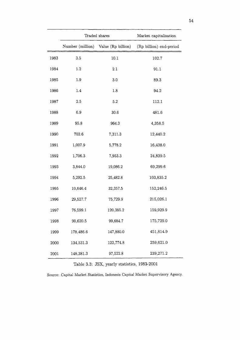
54
Traded shares Market capitalisation
Number (million) Value (Rp billion) (Rp billion) end-period
1983 3.5 1 0 .1 102.7
1984 1 .2 2 .1 91.1
1985 1.9 3.0 89.3
1986 1.4 1 .8 94.2
1987 2.5 5.2 1 1 2 .1
1988 6.9 30.6 481.6
1989 95.8 964.3 4,358.5
1990 702.6 7,311.3 12,440.2
1991 1,007.9 5,778.2 16,438.0
1992 1,706.3 7,953.3 24,839.5
1993 3,844.0 19,086.2 69,299.6
1994 5,292.5 25,482.8 103,835.2
1995 10,646.4 32,357.5 152,246.5
1996 29,527.7 75,729.9 215,026.1
1997 76,599.1 120,385.2 159,929.9
1998 90,620.5 99,684.7 175,729.0
1999 178,486.6 147,880.0 451,814.9
2 0 0 0 134,531.3 122,774.8 259,621.0
2 0 0 1 148,381.3 97,522.8 239,271.2
Table 3.3: JSX, yearly statistics, 1983-2001
Source: Capital Market Statistics, Indonesia Capital Market Supervisory Agency.

55
index fell back to 247 at the end of 1991 before taking off again in 1992 and reaching
a record 637 at the end of 1996.
3.3 Changes in monetary policy
M onetary policy focused until 1983 on credit controls (i.e. credit ceilings and
interest rate controls), which covered both private and State banks. These controls,
however, proved ineffective in constraining growth of the money supply or inflation.
This was epitomised by famous "incidents" (so-called "Pertam ina Crisis" in 1975,
reduction of the required reserve ratio from 30 percent to 15 percent in December
1977). Furthermore, the continuously positive balance of payments had an impact
on reserve, or base money and was a major factor in the expansion of money supply
(McLeod, 1993). W hen the oil boom ended in 1982, in parallel with the series of
market-oriented financial reforms, the approach of monetary policy began to shift
from direct to increasingly indirect instruments of intervention.
3.3.1 Policy objectives and intermediate targets
For the period 1983 to May 1999 (when the new central bank law was enacted),
the basic objectives of monetary policy in Indonesia, as stipulated in Act No. 13 of
1968 concerning the central bank, were to assist the government in (a) managing,
safeguarding and maintaining the stability of the Rupiah, and (b) facilitating the
production and development w ith the aim of promoting employment creation and
improving the living standards of the population. Accordingly, BI was responsible
for formulating and implementing monetary policy which was directed towards

56
1983 80.37
1984 63.53
1985 66.53
1986 69.69
1987 82.43
1988 305.12
1989 399.69
1990 417.79
1991 247.39
1992 274.33
1993 588.76
1994 469.64
1995 513.84
1996 637.43
1997 401.71
1998 398.03
1999 676.91
2 0 0 0 416.32
2 0 0 1 392.04
Table 3.4: JSX, yearly (end-period) composite share price index, 1983-2001
Source: Capital Market Statistics, Indonesia Capital Market Supervisory Agency.

57
achieving several objectives, namely controlling inflation, avoiding serious loss of
foreign exchange reserves, supporting investment in general, or in certain priority
areas of economic activity, and achieving relatively high economic growth so as
to increase per capita income (Iljas, 1998). BI sought to achieve these multiple
objectives primarily through control of monetary aggregates (M l, M2) at levels
th a t are adequate to support the targeted rate of economic growth. Under this
framework, monetary targets are the intermediate target to be influenced in turn
by controlling the amount of reserve money (MO—the operational target) through
open market operations. Monetary policy thus relied on the linkages between MO
and M 1/M 2 and between M1/M2 and the ultim ate objectives . 16
Although BI never published its monetary targets, McLeod (19996) reports
th a t targets were set for growth of M l and M2 of the order of 19-20 percent per
year in 1995, and it was assumed tha t there were reliable multipliers which would
enable these targets to be met through appropriate manipulation of base money.
The multipliers were 1.9 (m m i) and 7.8 (m m 2) a t March 1995 (Bank Indonesia,
1995).17 The required changes in base money were derived from
AM n = m m nA B, n = 1,2 (3.1)
where m m is the money multiplier which shows the changes in money (M l or
M2), AM n, for a given change in base money, A B.
16 Monetary aggregates in Indonesia are classified as follows: (1) Coins and currency in circulation; (2) MO: base money (cash plus the reserves of the commercial banks); (3) Ml (cash plus the non-interest bearing demand deposits at the commercial banks); and (4) M2 (Ml plus theinterest bearing time deposits at the commercial banks).
17 For comparison, the multipliers were about 1.4 (mmi) and 6.5 (7717712) at May 2004 (Bank Indonesia, 2004, p. 11, Graph. 22).
58
Hence the framework required stability of the money demand function, income
velocity and money multipliers.
3.3.2 Policy instruments
The PAKJUN policies allowed the State banks to raise their deposit and loan in
terest rates. The resulting imbalance between the deposit mobilising and lending
capabilities of the State and private banks stimulated the growth of the interbank
money market. In such context the monetary authorities undertook the devel
opment of an indirect instrument to influence the to tal supply of reserve money
in the banking system. In the absence of any government debt instruments, BI
introduced a new money market instrument in February 1984, called a Sertifikat
Bank Indonesia (SBI), which is a short-term liability of the Bank used to reduce
banking system liquidity (Binhadi and Meek, 1992). The SBIs have maturities
of 30 and 90 days and are sold each week through an auction. In early 1985, BI
introduced another money market instrument to increase banking system liquidity
called the surat berharga pasar uang (SBPU), which is a money market security
issued or endorsed by banks th a t BI is prepared to purchase at a discount from
the banks. The rate of discount is set by BI.
The two new instrum ents formed the new basis for m onetary policy to replace
direct bank lending controls, "a practical approximation to open market operations
in other countries where government debt is bought and sold by the central bank"
(McLeod, 1999a). In effect, BI takes part in the interbank m arket by buying up any
excess reserves from the banks through sales to them of SBIs and then supplying

59
reserves through discounting of their SBPUs. BI sets no limits on the amount of
SBIs it sells to the State banks, but it sets ceilings on the amount of SBPUs it buys
from each bank as a means of controlling the growth of reserve money. SBPUs are,
therefore, used primarily as quantitative instruments of monetary policy, to control
the supply of reserve money while the SBI is a fixed interest ra te instrum ent used
for liquidity adjustment, primarily by the State banks (Cole and Slade, 1996).
3.3.3 Reverting to direct controls: the Sumarlin shocks
The sharp decline in world oil prices in 1986-1987 and the combination of steady,
heavy losses on foreign exchange reserves and high interbank interest rates through
out this period eventually led the government to intervene in June 1987. The au
thorities implemented a dramatic contraction of domestic liquidity, which came to
be labeled "Sumarlin shock", after Sumarlin, the then Minister of Finance.
The liquidity contraction was accomplished by two specific measures. The first
was an instruction to four large State-owned enterprises to transfer part of their
tim e deposit balances at the State banks into holdings of new SBIs. The second
was a reduction in the ceilings on SBPUs discounted at the central bank to zero,
in effect forcing all the commercial banks to buy back their SBPUs from Bank
Indonesia. These measures wiped out, almost overnight, the equivalent of all the
available legal reserves of the banking system (Cole and Slade, 1996). As a result,
banks could only meet their reserve requirements by selling foreign exchange to BI,
or borrowing through the discount window. The use of the central bank facility,
however, was discouraged by an increase in the discount rate from 2 0 percent to

60
30 percent.
On 27 February 1991, a number of large State-owned enterprises were again
instructed to transfer their time deposits in banks into holdings of SBIs. The
amount transferred on 1 March 1991 was Rp8 trillion, equal to approximately one-
th ird of M l or three-quarters of reserve money. BI offered to purchase SBPUs from
the affected banks to offset 80 percent of their loss of funds. The net contractionary
effect on reserve money from this sale of SBIs and purchase of SBPUs was about
Rp2 trillion. This exceeded the total reserves of the banking system averaging
about R p l .6 trillion. As a result, both SBI and SBPU markets were reactivated,
allowing the central bank to have larger stocks of these instrum ents outstanding
with which to carry out money market operations. On the negative side, SBI rates
as well as bank deposit and loan rates were held at high levels throughout 1991.
Growth of total bank credit, which had averaged 51 percent per year in 1989-1990,
dropped to 16 percent in 1991 and 9 percent in 1992; private national bank credit
only increased by 1 percent in 1992, compared with average annual increases of
more than 80 percent in 1989-1990 (Cole and Slade, 1996, p. 61).
3.4 Crisis-driven reforms and policy changes
The Indonesian economic crisis started as a contagion of the Thai currency
crisis of July 1997. The complex chain of events th a t led to the crisis has been dis
cussed in a number of papers (see for instance Enoch et a l, 2003; Grenville, 2004).
The following discussion provides a brief overview of m onetary policy approach
during the crisis as well as crisis-driven changes to banking regulations.

61
80
70
60
50
40
30
20
10
0.a
Intertsank Bank D e p o s it S B I LIBOR
Figure 3.4: Key interest rates, 1983-2000
3.4.1 Floating of the Rupiah and third Sumarlin shock
Critical and far-reaching decisions were taken in the initial phase of the crisis,
before the involvement of the IMF towards the end of October 1997. The exchange
rate band was widened in July 1997 from 8 percent to 12 percent, to allow the rate
to move without requiring BI to use reserves in its defence. On 14 August 1997,
the Rupiah was floated. A few days later, a major contractionary open market
operation took place, which precedent was the earlier Sumarlin shocks. SOEs were
once again instructed to withdraw their bank deposits and use them to buy SBIs,
thereby raising concerns that banks would not have enough liquidity to meet either
their small reserve requirements or their daily cheque clearing obligations in the
payments system.
On 31 October 1997, a letter of intent from the Indonesian government to
the IMF set out a new IMF-endorsed monetary strategy. The main element of the

62
strategy was to set targets for the slow growth of base money (7 . 7 percent according
to Fane, 2000, p. 50) and its components—net domestic credit and net foreign
assets. The aim was to restore confidence in the Rupiah and cause a reversal of the
depreciation. Accordingly, BI followed a high interest rate policy and raised SBI
rates (the benchmark rates) several times (Figure 3.4). The rates increased from
the average 14 percent pre-crisis to 30 percent in December 1997, and 80 percent in
August 1998. As a result, the amount of interbank call money transactions surged
by 400 percent, from Rp0.5 trillion in 1996 to R p 2 trillion in 1997. The sale of SBI
also rose by four times in value, while SBPU rose by around 80 percent over the
same period (Halim, 2000). SBI rates were subsequently reduced to 40 percent in
March 1999 before returning gradually to their pre-crisis level.
Despite the base money targets and high interest rate policy, the exchange
rate of the Rupiah against the US dollar depreciated by almost 30 percent in
1998 from its 1997 value (by more than 80 percent in the first months of 1998),
and stabilised a t a much depreciated value in the first half of 1999. Between
September 1997 and September 1998, base money grew by 95 percent (Fane, 2000).
On the supply side the closure of 16 private banks in November 1997 caused runs
on individual banks and forced BI to provide bank liquidity support (Bantuan
Likuiditas Bank Indonesia or BLBI) amounting to around R pl50 trillion . 18 On
the demand side there was an im portant increase in the demand for currency from
the public, motivated by the loss of confidence in the banking system and rapidly
18 These liquidity injections were partly offset by net issue of SBIs and foreign currency intervention amounting to around RplO trillion (Halim, 2000).

63
rising prices. Currency in circulation doubled in the year to mid 1998, accounting
for 85 percent of the increase in base money (Grenville, 2 0 0 0 ).
3.4.2 Reforms to banking laws and regulations
The following discusses amendments to the 1992 banking law enacted in November
1997, the new central bank law enacted in May 1999, and various changes to
the banking prudential regulations introduced during 1998, drawing from McLeod
(19996).19
Amendments to the Banking Law introduced in November 1997 lifted the pre
vious requirement tha t the government retain majority ownership of State banks;
abolished regulations discriminating between domestic and foreign joint venture
bank (in particular, in relation to the expansion of their branch networks); and
allowed foreign banks as well as foreign non-bank financial institutions and cor
porations to acquire up to 1 0 0 percent of the shares in existing banks (including
the State banks). New clauses also provided the legal basis for the establishment
and operations of the Indonesian Bank Restructuring Agency (IBRA) and for the
establishment of a deposit insurance institution.
The central bank law enacted in May 1999 established the stability of the
Rupiah, in term s of both its purchasing power and its rate of exchange for other
currencies as the sole objective of BI. The law also imposed new constraints on
BI including the requirement th a t its monetary liabilities do not exceed its capital
by more than a factor of 1 0 ; the interdiction to acquire equity in other entities
19 Respectively, Law No. 10 1998 on Changes to Law No. 7 1992 on Banking, and Law No. 3 1999 on Bank Indonesia.

64
w ithout the approval of parliament; the interdiction to lend to the government, or
to purchase government bonds except in the secondary market; and the limitation
to a maximum of 90 days for the provision of credit to the banks as lender of last
resort. The new law also called for the transfer of the task of prudential supervision
of banks from BI to a new, independent institution, by the end of 2002.
BI decrees issued in November 1998 softened the existing prudential regula
tions. The decrees focused on capital adequacy (No. 31 /146/K E P/D IR );20 the
classification of assets by quality (No. 131/47/K E P/D IR ); the setting aside of
reserves against possible reductions in asset values (No. 31/148/K E P/D IR ) as
well as the procedures to be followed when restructuring borrowers’ debts (No.
31/150 /K E P /D IR ).
3.4.3 Impact of the crisis on the financial sector
The crisis had a significant impact on the banking system, which as mentioned
above held as much as 65 percent of the financial sector’s to tal assets in 1997.
The income of the banking system declined by 300 percent in 1997 (Halim, 2000).
Banks became incapable of performing their financial intermediary functions. The
sharp devaluation of the Rupiah against the US dollar caused investors, who had
borrowed in US dollars (about 30 percent of all bank loans) to default, as the
value of their collateral was now very much below the value of their loans .21 High
20 The minimum required capital adequacy ratio was reduced from 8 percent before the crisis to 4 percent. Moreover, banks were permitted to include part of their loan loss provisions in this figure.
21 In July 1998, the Asset Management Unit (AMU) was established as part of IBRA to handle non-performing loans from banks.

65
interest rates also encouraged defaults. November 1997 saw the liquidation of 16
banks. In February 1998, IBRA intervened in 54 weak banks, whose BI emergency
borrowings exceeded 2 0 0 percent of their capital and whose capital was less than 5
percent of their assets. In April 1998 IBRA suspended 7 banks whose borrowings
exceeded 500 percent of their capital, and more than 75 percent of their assets. In
M arch 1999 38 banks were closed, 9 banks recapitalised and 7 banks were taken
over by IBRA.
The crisis also had a significant impact on the capital market. There was a
m ajor decline in foreign and domestic portfolio investment (Table 3.2). The share
of transactions by foreign investors fell from 52 percent in 1997 to 42 percent the
next year and was just under 11 percent in 2001. The to tal value of stock market
transactions fell from Rpl20 trillion in 1997 to Rp99 trillion the next year. Market
capitalisation fell by about 35 percent in 1997 compared to 1996 (Table 3.3). Based
on the Price Earning Ratios, the average stock market price was halved, from 21.6
to 10.5, with many share prices below Rp500, about two cents at Rp8,500 per
US dollar (Halim, 2000) . 22 As share prices fell, the composite share price index
plunged from 637 points at the end of 1996 to only 402 points at the end of 1997
and just under 400 points at the end of 1998 (Table 3.4). Despite a recovery to
around 678 points at the end of 1999, it plunged again to 416 points at the end of
2000 and reached 392 points a t the end of 2001.
22 The Price Earning Ratio (PER) is the ratio of the regular closing price over the earnings per share (EPS). The latter is derived by dividing net profit (after taxation) by the number of shares issued.

CHAPTER 4
FINANCIAL LIBERALISATION AND STRUCTURAL BREAKS IN
MONETARY AGGREGATES AND THE DETERMINANTS OF MONEY
DEMAND IN INDONESIA
4.1 Introduction
Many experts claim tha t the process of financial liberalisation experienced by
Indonesia since 1983 has caused instability in the money dem and function some
where in the 1990s (see for instance Alamsyah et al., 2001). However, there has
been no systematic attem pt at corroborating such claim. In addition, the issue of
whether any potential instability in the money demand relationship is a temporary
or a permanent phenomenon has been largely ignored.
In this chapter we want to investigate this claim. We start from the obser
vation th a t there are not many results on the time series properties of monetary
aggregates and the determinants of money demand in Indonesia. Previous stud
ies including inter alia Tseng and Corker (1991); Price and Insukindro (1994);
Dekle and P radhan (1997; 1999); and Chaisrisawatsuk et al. (2004) model these
series as unit root processes. This practice, however, suffers from two im portant
caveats. First, neglecting the possible presence of structural breaks might bias the
results of unit root tests towards a failure to reject the unit root null hypothe
sis. Perron (1989); Rappoport and Reichlin (1989); and Hendry and Neale (1991)

67
have shown tha t (i) structural change/regime shifts can mimic unit roots in sta
tionary autoregressive time series; (ii) such shifts are very hard to detect using
conventional parameter constancy tests. Second, applying the conventional inte
gration/cointegration approach if the series are actually stationary around broken
deterministic trends can give misleading results (Leybourne and Newbold, 2003).
Since the detection of structural break in economic variables crucially depends
on the maintained hypothesis about the dynamics of the variables into question, we
apply the univariate method proposed by Vogelsang and Perron (1998) designed
to detect structural breaks on nine series in a standard specification for money de
m and using Indonesian data spanning from 1983:1-2001:4. This statistical method
can detect single breaks of unknown timing in both the intercept and slope of the
trend function of the series, assuming each of them follows a simple auto-regressive
(AR) process . 1
Finally, unlike previous studies of the demand for money in Indonesia, the
sample period covers the four critical quarters—the last two quarters of 1997 and
the first two quarters of 1998—often dubbed the "crisis period" in the Indonesian
economic crisis literature (Grenville, 2000; Fane, 2000).
Structural change would be quite perilous to ignore. Inferences about the
money demand relationship could go astray, forecasts could be inaccurate and
policy recommendations could be misleading. We find evidence in favour of a
1 While this approach is the most advanced method to endogenously detect structural breaks, it is unable to identify multiple structural breaks. As Ben-David and Papell (1998) note, tests that allow for multiple structural breaks, such as Bai and Perron (1998, 2003), are restricted to stationary and non-trending data, which is not the case for the variables under investigation in this study.

68
structural break in all the series except the three monetary aggregates (MO, M l,
and M2). Moreover, we find th a t the break for most series occurs around the end
of 1997 and coincides with the crisis and a major government intervention in the
money market for which the precedent is the Sumarlin shock of 1991 (discussed in
the previous chapter).
The rest of the chapter is organised as follows. Section 4.2 presents the
Vogelsang-Perron methodology. Section 4.3 discusses the empirical results. Section
4.4 offers some concluding remarks.
4.2 Methodology
To detect structural breaks in our series, we apply the procedure outlined in
Perron (1989), Zivot and Andrews (1992), and Vogelsang and Perron (1998) (VP
hereafter). These authors have shown that the presence of structural breaks, if
ignored, bias standard unit root tests towards the acceptance of the unit root
hypothesis. VP have developed unit root tests which allow for the possibility
of a structural break in the deterministic trend and in which the breakdates are
endogenously determined. The null hypothesis is tha t of a unit root against the
alternative of stationarity w ith a break in the intercept and slope of the trend
function.
Throughout, Tb denotes the time at which the change in the time function
occurs. The first model allows only a shift in the intercept under both the null
and alternative hypotheses (crash model). Under the second model, both a shift
in intercept and slope are allowed at time Tb (crash/changing growth model). The
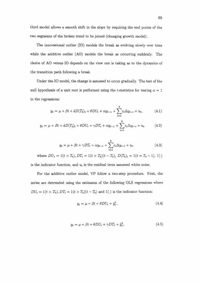
69
third model allows a smooth shift in the slope by requiring the end points of the
two segments of the broken trend to be joined (changing growth model).
The innovations] outlier (10) models the break as evolving slowly over time
while the additive outlier (AO) models the break as occurring suddenly. The
choice of AO versus 10 depends on the view one is taking as to the dynamics of
the transition path following a break.
Under the 10 model, the change is assumed to occur gradually. The test of the
null hypothesis of a unit root is performed using the ^-statistics for testing a = 1
in the regressions:
k
Vt = M + fit + dD(Tb)t + ODUt + ocyt- 1 + CiAyt~i + ut , (4-1) i= 1
k
yt = y + (3t + dD(Tb)t + ODUt 4- 7 DTt 4- ctyt-i + ^~^CjAyt-i + ut . (4-2)i = l
k
yt = y + pt + 7 DTt + ay t-i + ^>2ciA y t-i + ut . (4.3)i= 1
where DUt — 1 (t > Tb),D T t = 1 (t > Tb)(t - Tb), D (Tb)t = 1 (t = Tb + 1 ), 1 (.)
is the indicator function, and ut is the residual term assumed white noise.
For the additive outlier model, VP follow a two-step procedure. First, the
series are detrended using the estimates of the following OLS regressions where
DUt = 1 (t > Tb), D Tt = 1 (t > Tb)(t — Tb) and 1 (.) is the indicator function:
yt = fi + p t + 9DUt + y] , (4.4)
yt = m + fit + ODUt + 7 DTt + yt 1 (4.5)

70
yt = fi + fit + ^D T t + yt3, (4 .6 )
The test of the null hypothesis of a unit root is then performed using the
t-statistic for testing a = 1 in the regressions:
k k
yi = ^ 2 ^ iD { T b)t-i + a y l^ 4- + uu (j = 1,2) (4.7)2 = 0 1=1
k
Vt = ay? - 1 + Y l^ y t - i + Ut’ (4-8)1= 1
where D (Tb)t = l ( t = Tb + 1 ) and ut is the residual term assumed white noise.2
In all the regressions Tb (the breakdate used), and k (the lag length of the
autoregression) are treated as unknown.
For all the statistics, the appropriate values of the breakdate and the truncation
lag param eter are unknown. Various data-dependent methods to select these values
endogenously. VP propose two approaches for choosing Tb. The first approach
involves choosing Tb such tha t the statistics t& is minimised. This choice of Tb
corresponds to the breakdate th a t is more likely to reject the unit-root hypothesis.
The second approach involves choosing Tb to maximise some statistics tha t tests
the significance of one or more of the break parameters (0,7). For the AO and
10 Models 1, Tb is chosen using the maxima of t& and |£a|- The maximum of
\tg\ is used when the direction of the break is unknown while the maximum of t-e
is used when the direction of the break is known a priori to be positive. If the
direction of the break is known to be negative, then the minimum of t~e is used.
2 The one-time A:-h 1 dummy variables D (Tb) t - i (i = 0,..., k) in (4.7) are not needed in Model3 as the t-statistic on a is asymptotically invariant to the correlation structure of the data withthe appropriate choice of k (see Perron and Vogelsang (1993a) for details).
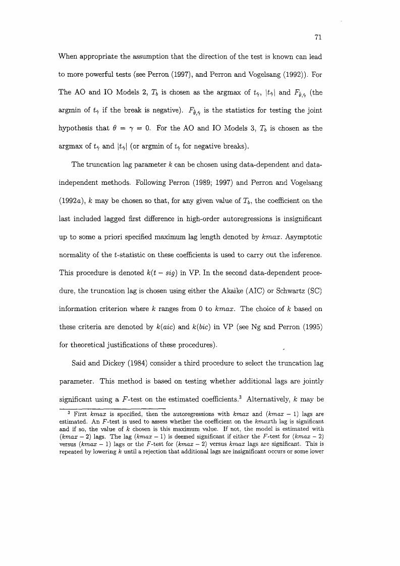
71
When appropriate the assumption that the direction of the test is known can lead
to more powerful tests (see Perron (1997), and Perron and Vogelsang (1992)). For
The AO and 10 Models 2 , T*> is chosen as the argmax of ty, \t^\ and (the
argmin of ty if the break is negative). is the statistics for testing the joint
hypothesis th a t 6 = 7 = 0. For the AO and 10 Models 3, Tb is chosen as the
argmax of ty and \t^\ (or argmin of ty for negative breaks).
The truncation lag parameter k can be chosen using data-dependent and data-
independent methods. Following Perron (1989; 1997) and Perron and Vogelsang
(1992a), k may be chosen so that, for any given value of Tj,, the coefficient on the
last included lagged first difference in high-order autoregressions is insignificant
up to some a priori specified maximum lag length denoted by km ax. Asymptotic
normality of the t-statistic on these coefficients is used to carry out the inference.
This procedure is denoted k(t — sig) in VP. In the second data-dependent proce
dure, the truncation lag is chosen using either the Akaike (AIC) or Schwartz (SC)
information criterion where k ranges from 0 to km ax. The choice of k based on
these criteria are denoted by k(aic) and k(bic) in VP (see Ng and Perron (1995)
for theoretical justifications of these procedures).
Said and Dickey (1984) consider a third procedure to select the truncation lag
parameter. This method is based on testing whether additional lags are jointly
significant using a F -test on the estimated coefficients.3 Alternatively, k may be
3 First km ax is specified, then the autoregressions with km ax and (km ax — 1) lags are estimated. An F-test is used to assess whether the coefficient on the km ax th lag is significant and if so, the value of k chosen is this maximum value. If not, the model is estimated with (kmax — 2) lags. The lag (kmax — 1) is deemed significant if either the F-test for (km ax — 2) versus (km ax — 1) lags or the F-test for (kmax — 2) versus kmax lags are significant. This is repeated by lowering k until a rejection that additional lags are insignificant occurs or some lower

72
determined a priori, by treating it as a fixed function of the sample size T, thus
specifying a choice of the parameter independent of the data. However, as argued
in Perron (1997), there is some evidence tha t using data-dependent methods to
select the truncation lag parameter leads to test statistics having better properties
(size and higher power) than if a fixed k is chosen a priori (unless of course the
value of k which is best happens to be selected).
4.3 Empirical results
It seems reasonable to allow a structural change to take a period of time to take
effect. In w hat follows we focus on the Vogelsang and Perron 10 Model 2 (Zivot and
Andrews Model C) in which the break occurs gradually. Model 2 (crash/changing
growth) is chosen because it encompasses Model 1 (crash) and Model 3 (changing
growth). The series considered are RMO (real MO), RM 1 (real M l), RM2 (real
M2), RGDP (real GDP), MMR (money market rate), TD R (3 months time deposit
rate), USTBR (3 months US T-bill rate), INF (inflation rate), NCDR (currency,
depreciation rate in nominal terms), RCDR (currency depreciation rate in real
terms). These series have been used in the conventional specification of the money
demand function for Indonesia. All variables are measured in levels and converted
to logs (see Appendix A for details). The series are shown in Figure 4.1. For
completeness, additional results for Model 2 when the break is modelled as an
additive outlier (i.e. occurs suddenly) are provided in Appendix B .4 It is worth
bound is attained.4 Results for the AO Models 1 and 3 are also available upon request.

264
25 B.
25 B.
272.
266.
260.
29 2
275.
26£.
31X3.
E 3
I MMRl
.11
.10.
JOB,
08.
07.
06.
£5.
JM.
03.
02.
020
016.
£06 .
USTBRl
3RCOR]
Figure 4.1: Plots of the time series

74
noting th a t the results obtained under the AO assumption are by and large similar
to those obtained under the 10 assumption.
We estim ated the 10 Model 2 equation described in the previous section over
all possible breakdates, TU
k
Vt = M + fit 4- dDt 4- 6DUt + 7 DTt 4- otyt - 1 + '^^4>iA y t_i 4- ut (4.9)i = 1
where DUt = 1 for t > Tb, 0 otherwise, D t = l , t = Tb, 0 otherwise, D Tt = (t -
Tb) for t > Tb, 0 otherwise, and u t is the residual term assumed white noise, k is the
optimal lag length, and following Perron (1989; 1997), and Perron and Vogelsang
(1992), k is selected using the significant t method. S tarting with maximum lag
length of 9, Equation (4.9) is estimated for each breakdate.5 Using the appropriate
lag length, Equation (4.9) is estimated sequentially over all possible breakdate T&,
Tb = k0, ...,T — k0, where k0 = 5T , T is the sample size and 5 is the trimming
param eter adopted. Here, T = 76 for each series, and we set £ = 0.20 so that Tb =
1986:3,..., 1998:2.6 The date of the break is chosen in three different ways, using
the argmin of £y, the argmax of \t^ \ , and the argmax of F-e .. After identifying the
appropriate breakdate, the unit root hypothesis is tested using the t-statistic for
a = 1. Perron (1997) reports finite sample critical t-values for testing a = 1 when
the breakdate is chosen using the argmin of t^ and argmax of |£^,|, and Vogelsang
5 The choice of the maximum lag length is somewhat arbitrary. As Perron (1997) argued, on the one hand, one would like a large value to have as unrestricted a procedure as possible. On the other hand, a large value yields problems of multicollinearity in the data and also a substantial loss of power.
6 Some trimming is required because in the presence of the endpoints of the sample, the asymptotic distribution of the statistics diverges to infinity. Consequently, the procedures cannot pick up any breaks in the series occurring before the third quarter of 1986, which could possibly be related to the June 1983 reform package discussed in the previous section.

75
and Perron (1998) report finite sample critical values when the breakdate is chosen
using the argmax of F-e -.
The results for each series are reported in Tables 4.1-4.3.7 Note first tha t the
null hypothesis of a unit root in RMO, RM1, RM2, and USTBR cannot be rejected,
even at the 10% level, irrespective of the method chosen to select the breakdate.
In contrast, we can reject the unit root null for NCDR and RCDR in all three
cases. When the breakdate is chosen using the argmin of ty, the unit root null is
only rejected for two series, NCDR and RCDR. Note th a t this is not surprising as
the selection procedure imposes the a priori restriction th a t the direction of the
break is negative, which is unlikely with MMR, TDR, and INF. The breakdates
for RCDR coincide and show a break located in the third quarter of 1997.
The estimated breakdates for NCDR are located in the second and third quar
te r of 1997.8 Consider now the case where the procedures to select the breakdate
do not impose the restriction of a one-sided change, th a t is, when the break is
chosen by maximising \t^\ (as shown in Table 4.2) or by maximising Fq^ (as shown
in Table 4.3).
The unit root null hypothesis is now rejected for three more series, MMR,
TDR, and INF. The breakdate for MMR is located in the second quarter of 1997,
7 All unit root tests are performed using GAUSS 6.0 for Windows, kernel review 6.0.8, GUI review 6.0.3 and the procedures included in Blini version 1.03 by Charemza and Makarova (2002).
8 While the second quarter of 1997 does not exactly correspond to the start of the Asian crisis (i.e. third quarter of 1997), the economic interpretation remains the same. The selection of 1997:2 is due to the presence of the dummy variable Dt in (4.9). Hence, 1997:2 may be chosen because the dummy variable takes value 1 in 1997:3 and offers some additional fit to the 1997:3 crash over what the change in the intercept can do alone.

76
H ttf ■̂ 0,7 t& Break date
RMO 0.94 3.22 4.89 -2.00 1989:1
RM1 1.48 0.37 1.85 -1.74 1988:1
RM2 1.65 1.55 1.29 -0.15 1986:3
RGDP -1.30 3.44 5.87 -3.89 1994:3
MMR -0.58 1.89 1.72 -3.45 1993:1
TD R -1.20 1.51 1.11 -3.19 1994:3
USTBR -0.30 0.98 0.46 -1.80 1992:2
INF -0.24 1.26 0.80 -3.82 1992:4
NCDR -7.11 6.67 24.02 -8.52+ 1997:3
RCDR -8.28 7.68 32.40 -9.57+ 1997:3
Table 4.1: 10 Model 2 results
Choosing the breakdate minimising t^
Notes: t denotes rejection of the unit root null hypothesis at the 0.01 nominal testsize. Critical values of the t& statistics are from Perron (1997), Table 1 (usingT=100).

77
H t*, t^ Break date
RM0 0.94 3.22 4.89 2.00 1989:1
RM1 1.94 4.08 8.27 4.23 1996:1
RM2 1.04 3.76 6.73 3.31 1996:1
RGDP 1.30 3.44 5.87 3.89 1994:3
MMR 11.20 6.40 58.87 9.31* 1997:2
TD R 5.89 4.72 16.48 5.12+tt 1998:1
USTBR 1.79 2.19 2.46 1.88 1998:1
INF 12.27 10.45 70.91 12.97* 1997:3
NCDR 7.11 6.67 24.02 8.52* 1997:3
RCDR 8.28 7.68 32.40 9.57* 1997:3
Table 4.2: 10 Model 2 results (continued)
Choosing the breakdate maximising
Notes: j and Iff denote rejection of the unit root null hypothesis at the 0.01 and0.10 nominal test size respectively. Critical values of the t& statistics are fromPerron (1997), Table 1 (using T=100).

78
while the breakdate for TDR is located in the first quarter of 1998.9. The null of a
unit root in RGDP is also rejected when the break is chosen by maximising Fq~,
w ith the estimated breakdate located in the fourth quarter of 1997.
Overall, the results show tha t the null hypothesis of a unit root can be rejected
for six out the nine Indonesian series under investigation. W hen the unit root
hypothesis is rejected, the date of the break suggests in most cases a shift located
in one of the four quarters of the crisis.
For comparison only, the test proposed by Leybourne (1995) is also used. The
results are shown in Table 4.4. The test is based on forward and reverse augmented
Dickey-Fuller (ADF) regressions. Critical values are obtained from Leybourne
(1995, p. 565). Leybourne showed that this test offers a 15 percent increase in
power relative to the standard ADF test. The unit root hypothesis is rejected for
MMR, TDR, INF, NCDR, and RCDR, but not for RGDP.
4.4 Conclusions
Previous studies of money demand in Indonesia have worked under the main
tained assumption th a t the trend in the series which enter the money demand
function could be characterised as a random walk. The hypothesis of a random
walk trend implies th a t the sum of the autoregressive coefficients equals one. In
other words there is a unit root in the autoregressive polynomial. The implication
of this hypothesis is th a t the trend is moved by random shocks and then stays at
the new level until disturbed by another random shock.
9 See previous footnote.

79
h t^ •^,7 ta Break date
RM0 0.60 3.01 4.94 -3.03 1992:1
RM1 -4.29 -0.66 17.71 -3.60 1998:1
RM2 -2.70 -1.48 7.50 -2.58 1998:1
RGDP 13.21 -1.71 81.96 -7.18+ 1997:4
MMR 11.20 -6.40 58.87 -9.31+ 1997:2
TD R 5.89 -4.72 16.48 -5.12+++ 1998:1
USTBR 3.18 -1.09 4.82 -2.35 1996:1
INF 12.27 -10.45 70.91 -12.97+ 1997:3
NCDR -7.32 6.24 25.26 -8.58+ 1997:2
RCDR -8.28 7.68 32.40 -9.57+ 1997:3
Table 4.3: 10 Model 2 results (continued)
Choosing the breakdate maximising F~e ^
Notes: f and fff denote rejection of the unit root null hypothesis at the 0.01 and0.10 nominal test size respectively. Critical values of the t& statistics are fromVogelsang and Perron (1998), Table 3 (using T=100).

80
ADFmax
RMO -1.68
RM1 -1.48
RM2 -0.29
RGDP -1.64
MMR -2.49tf
TDR -2.64+t
USTBR -0.69
INF -2.76tf
NCDR -2.45ft
RCDR -3.141
Table 4.4: Leybourne (1995) unit root tests
Notes: An intercept and trend are included in the Dickey-Fuller regressions for RMO, RM1, RM2, RGDP. An intercept only is included in the Dickey-Fuller regressions for MMR, TDR, USTBR, INF, NCDR, and RCDR. f and tt denote rejection of the unit root null hypothesis at the 0.01 and 0.05 nominal test size respectively (using T=100). Critical values of the ADFmQX statistics are obtained from Leybourne (1995).
Our results challenge this assumption by providing empirical evidence that for
most of the series, the movement of the trend can be explained by a single struc
tural break in an otherwise constant linear trend. This explanation is plausible
since a trend break produces serial correlation properties tha t are similar to those
of a random walk. In effect, the results reverse inference for six out of the nine
Indonesian series under investigation. For these series, the timing of the break
typically occurs at the end of 1997 and coincides with the crisis and a major gov
ernment intervention in the money market for which the precedent is the Sumarlin
shock of 1991. The results do not reverse inference for the real money stock vari
ables (MO, M l, and M2). One im portant implication is tha t the series, with the
exception of the monetary aggregates, should not be differenced to achieve station-
arity. Instead, they should be detrended using the estimated breakdates. Another
implication concerns the significance of the coefficients, which can be tested us
ing the standard Student t distribution. Finally, the finding th a t the series are
stationarity after accounting for structural change possibly simplifies the query re
garding the predictability of the variables entering the money demand function by
removing some of the problems associated with forecasting from nonstationary se
ries. The results also suggest tha t the cointegration analyses of previous studies of
Indonesian money demand, which treated all the variables as unit root processes,
could be based on regressions containing mixtures of (trend-break) stationary and
nonstationary variables. The findings of such studies should therefore be taken
with some caution.

82
Appendix A: D ata definitions and sources
For each series the sample period is 1983:1-2001:4. The series are all seasonally
adjusted (with the exception of the three interest rate series).10
(1) RMO, RM1, and RM2 are the natural logarithms of the MO, M l and M2
definitions of the money stock (in billion rupiahs), each deflated by the consumer
price index (1995=100). Source: Bank Indonesia (unpublished).
(2) RGDP is the natural logarithm of the Indonesian gross domestic product
at 1995 m arket prices (in billion rupiahs). Source: Bank Indonesia (unpublished).
(3) MMR is the nominal money market rate, TDR is the nominal time deposit
rate (3 months), USTBR is the nominal US T-bill rate (3 months). The quarterly
rate is computed as:
0.25 * l [ l + (Rt/100)],
where R t is either one of the interest rates above. Source: IMFs International
Financial Statistics. INF is the inflation rate, computed as:
l(C P It) - l ( C P I t^ ) ,
where C P It is the consumer price index (1995=100). Source: IMFs Interna
tional Financial Statistics. NCDR is the currency depreciation rate in nominal
10 The seasonal adjustment is performed using the Stamp package (see Koopman, Harvey, Doornik and Shephard, 1995). We adopted the Stamp manual’s recommended version (p. 88) of the basic structural model of a stochastic trend with a stochastic slope, a trigonometric seasonal and an irregular component. A cyclical component was not included in the adjustment procedure. It is worth noting the Stamp manual’s comment (p. 88) that in practice seasonal components seem to be insensitive to the specification of the trend and the inclusion of a cycle.

83
term s, com puted as:
where E t is the nominal Rupiah exchange rate defined as the foreign price of
domestic currency (indirect quotation, a rise represents an Indonesian currency
appreciation). Source: IMFs International Financial Statistics. RCDR is the cur
rency depreciation rate in real terms, computed as:
[/(W P It) - l(W P I\) + l(E t)] - \l(W P It^ ) - l{ W P I l , ) + /(£ ,_ ,)],
where W P It is the domestic wholesale price index (1995=100), and W P I* is
a weighted average of foreign wholesale price indices (1995=100) computed as:
m r
W P I; = Y lw 'jW P ijt ,3 = 1
where Wj are fixed weights and m T = 4.
The four chosen countries account for half of Indonesia’s trade over the period
1997-2001. Each of the weights is computed as the average of annual trade with the
country divided by annual trade with all four countries over the period 1997-2001.
The countries and weights in brackets are: Japan (0.4025), the United States
(0.2642), Singapore (0.2058) and Korea (0.1275). Sources: IMFs International
Financial Statistics and United Nations Yearbook 2001.

84
Appendix B: Additional results
Additional results for Model 2 when the break is modelled as an additive outlier
are reported in Tables 4.5-4.7 below.
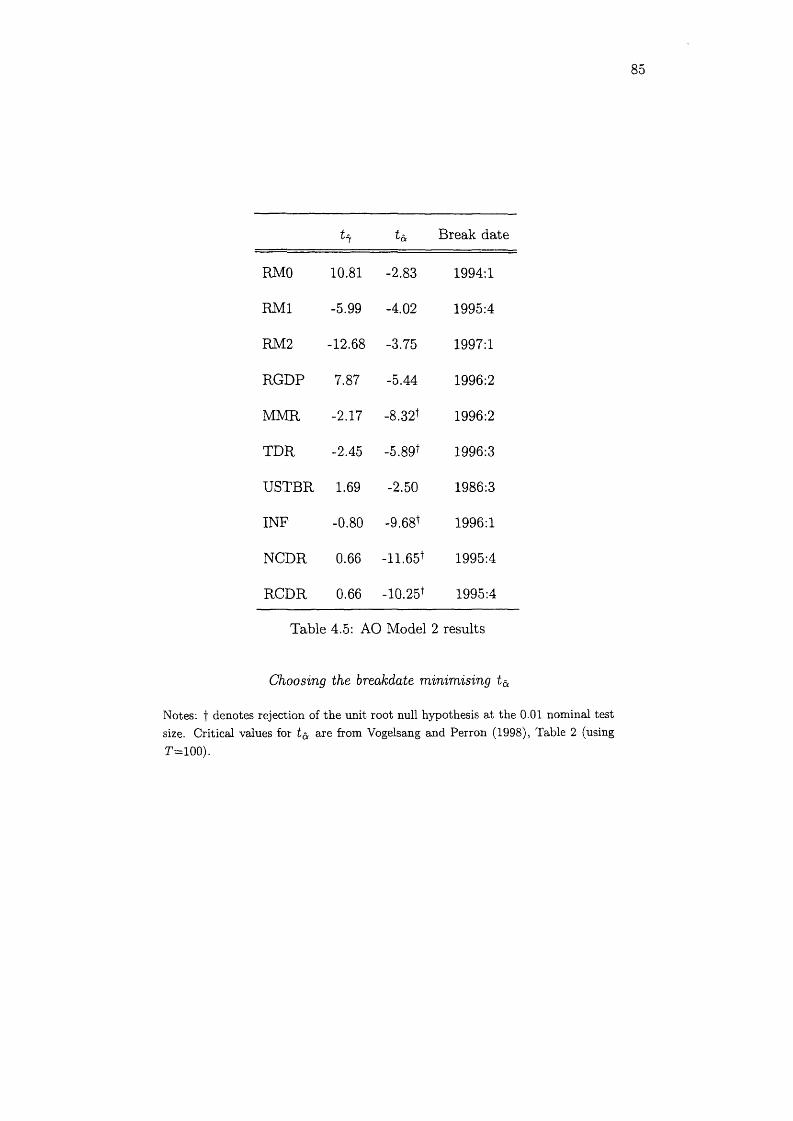
85
ttf ta Break date
RMO 10.81 -2.83 1994:1
RM1 -5.99 -4.02 1995:4
RM2 -12.68 -3.75 1997:1
RGDP 7.87 -5.44 1996:2
MMR -2.17 -8.32+ 1996:2
TDR -2.45 -5.89+ 1996:3
USTBR 1.69 -2.50 1986:3
INF -0.80 -9.68+ 1996:1
NCDR 0.66 -11.65+ 1995:4
RCDR 0.66 -10.25+ 1995:4
Table 4.5: AO Model 2 results
Choosing the breakdate minimising t&
Notes: f denotes rejection of the unit root null hypothesis at the 0.01 nominal testsize. Critical values for 15. are from Vogelsang and Perron (1998), Table 2 (usingT = 100).

86
ta Break date
RMO 13.16 -2.51 1992:2
RM1 1.65 -2.08 1989:1
RM2 -0.35 -1.87 1985:3
RGDP 11.35 -3.59 1994:1
MMR 1.76 -3.37 1992:4
TDR 0.46 -3.31 1993:4
USTBR 4.89 -1.73 1992:4
INF 1.02 -3.54 1986:2
NCDR 2.66 -7.23* 1997:2
RCDR 3.21 -7.27* 1997:2
Table 4.6: AO Model 2 results (continued)
Choosing the breakdate maximizing t^
Notes: t denotes rejection of the unit root hypothesis at the 0.01 nominal test size. Critical values for t& are from Vogelsang and Perron (1998), Table 2 (using T = 1 0 0 ) .

87
t^ t& Break date
RMO 13.16 2.51 1992:2
RM1 6.05 3.27 1996:2
RM2 13.38 3.30 1996:3
RGDP 11.35 3.59 1994:1
MMR 9.74 4.69 1997:3
TDR 8.41 2.68 1998:2
USTBR 4.89 1.73 1992:4
INF 5.53 6.90t 1997:4
NCDR 2.66 7.23* 1997:2
RCDR 3.21 7.27* 1997:2
Table 4.7: AO Model 2 results (continued)
Choosing the breakdate maximising \ty\
Notes: f denotes rejection of the unit root hypothesis at the 0.01 nominal test size. Critical values for t & are from Vogelsang and Perron (1998), Table 2 (using T=100).

CHAPTER 5
FINANCIAL LIBERALISATION AND REGIM E SHIFTS IN INDONESIAN
MONEY DEMAND
5.1 Introduction
Previous money demand studies for Indonesia (e.g. Dekle and Pradhan, 1999;
Agrawal, 2001; Chaisrisawatsuk et al., 2004) th a t used cointegration analysis are
somewhat inconclusive. These studies, however, have not considered the possibility
th a t financial liberalisation may be associated with structural change, in which
case standard cointegration tests could yield misleading results (Leybourne and
Newbold, 2003).
Several tests have been recently developed in the statistical literature for test
ing cointegration in the presence of breaks bu t there is no consensus yet about
which is more powerful and offers more robust results (Jimeno et al., 2006). To
detect common structural breaks we apply the residual-based cointegration test
with regime shifts of Gregory and Hansen (1996). This test has been used inter
alia by Siddiki and Morrissey (2006) to investigate the stability of the demand for
money in three South Asian countries (Bangladesh, India and Pakistan).
The test has two main advantages: (i) it is more powerful than standard
residual-based tests for cointegration, which presume tha t the coefficients are time-
invariant under the alternative hypothesis; and (ii) the timing of the break is en
dogenous, which prevents informal data analysis from contaminating the choice

89
of breakpoint. We follow a three-step strategy. First, we test for cointegration
using a cointegrated vector autoregression (VAR) framework, assuming that the
full system can be partitioned into a vector of endogenous variables and a vector
of weakly exogenous variables. Second, we test for weak exogeneity of the condi
tioning variables in the long-run real money demand function. We show tha t the
weak exogeneity hypothesis cannot be rejected and reduce the full system model
to a conditional model, which increases efficiency and can be given a structural
interpretation (Johansen, 1992a). Finally, we test for cointegration between the
variables in the real money demand function allowing for the possibility of a shift of
unknown timing in the cointegration vector using the test of Gregory and Hansen
(1996). Unlike previous studies of Indonesian money demand, the sample period
covers the critical quarters of the 1997-98 economic crisis.
The results show tha t the money demand function is cointegrated in the pres
ence of structural breaks occurring (i) in the second quarter of 1991 and coinciding
with the Sumarlin shock and (ii) in the last quarter of 1997 and coinciding with the
crisis and a government intervention in the money market for which the Sumarlin
shock of 1991 is the precedent (all discussed in chapter 3).
The rest of the chapter is organised as follows. Section 5.2 describes the model
and methodology. Section 5.3 provides empirical results. Section 5.4 offers some
conclusions.
90
5.2 Methodology
We start the following conventional theoretical money demand function (see
for instance Goldfeld, 1992)
where m t is the money supply, yt is the scaling variable, the vector of interest rates,
R*, measures the yields on financial assets, the overall inflation rate, A p t ,measures
the return to holding goods, and the real exchange rate, et , captures the attrac
tiveness of holding foreign assets.
Since money demand is not directly observable, it is assumed tha t the money
market is always in equilibrium and tha t the money supply is exogenous. Thus,
one can identify the money demand function and use the quantity of money to
measure the demand for money (see for instance Laidler (1993) for a discussion of
the identification problem of the money demand function).
The money demand function in (5.1) has the following semi-logarithmic spec
ification
tyh fmijPti Vti R t, Apt, et) (5.1)
(m - p)t = PyVt + /3 rR t + pApt + Peet + intercept (5.2)
Defining the vector zt containing the n potentially endogenous variables dis
cussed above as
zt = [(m - p )t , yt, R t, Apt, e j ' = [(m - p)t , x t]' (5.3)

91
Assuming th a t the time series properties of the variables included in zt can
be well approximated by a log-linear unrestricted vector autoregression (VAR)
involving up to k lags of z t and augmented with intercepts and trends gives:
z t = AiZt_i + . . . 4- A k z t- k 4- + u t (5.4)
where u t ~ IN (0 , J2), z t is (n x 1), and each of the A * is an (n x n) matrix of
parameters.
The system is in reduced-form with each variable in z t regressed on only lagged
values of both itself and all the other variables in the system. Thus, ordinary least-
squaxes (OLS) is an efficient way to estimate each equation comprising (5.4) since
the right-hand side of each equation in the system comprises a common set of
lagged regressors.
Equation (5.4) can be formulated into a vector equilibrium correction model
(VECM) form:
Az* = IfiA zt-i 4 ... 4 r fcA zt_fc+1 4- n z t_fc 4 - \I>Dt 4 - u t (5-5)
where R = —(I — A i — ... — Aj) (i = 1,..., k — 1), II = —(I — A x — ... — A^) and
u* -m(o,i;).This way of specifying the system contains information on both the short-run
and long-run adjustment to changes in z t , via the estimates of F and II, respectively,
where II = a/3 ', a represents the speed of adjustment to disequilibrium and (3 is
a m atrix of long-run coefficients such that the term f3'zt- k embedded in (5.5)
represents up to r < (n — 1) cointegration relationships, which ensures tha t the z t
converge w ith their long-run steady-state solutions.

92
Estim ates of a and (3 can be obtained using the Johansen method of reduced
rank regression. Furthermore, Johansen (19926) shows th a t if the variables in x*
are weakly exogenous with respect to the param eters of the model (i.e., the T*, II,
a , /3), there will be no loss of information in modelling the change in real money
balances A (m t — p t) in the context of a conditional single-equation model of the
type:
f c - i f c - i
A (m - p )t = ^ J * A ( r a - p)t_i + Y j y 'A x t-i + a ((m - p )t_i - /5'xt_i) + eu (5.6)i = l i =0
where et ~IID (0, cr2).
The param eter a captures a feedback effect on the change in money holdings,
A (m — p)t , from the lagged deviation from the long-run target money holdings,
{(m — p) — (m — p)*)t~i- The target (m — p)*t is defined as a linear function of the
forcing variables x t , tha t is, as (m — p)*t = /^Xj.
It is hypothesised th a t the long-run money demand relationship embedded in
(5.6) may have shifted at some unknown point in the sample.
The above proposition cannot be tested with standard residual-based tests for
cointegration since they presume tha t the cointegration relationship is time in
variant under the alternative hypothesis. Gregory and Hansen (1996)—hereafter
GH—propose a class of residual-based tests allowing for a break in the intercept
and/or the slope vector in the cointegration relationship. These tests are non-
informative with respect to the timing of the regime shift, thus preventing infor
mal data analysis (such as the visual examination of the time series plots) from
93
contam inating the choice of breakpoint.
Following GH, the long-run (static) money-demand function embedded in (5.6)
is rew ritten with the (5 vector separated into the intercept and slope parameters
(i9, /3) as:
(m - p)t = 0i + 02<ptk + M + p [ x t + (ftkP'2x t + nt (5.7)
where n t is a stationary error term.
Structural change is included through the dummy variable:
10 if t < k
(5.8)
1 if t > k
where k is the unknown date of the (potential) structural break. Equation (5.7)
allows for three alternatives if (m — p)t and xt cointegrate: (i) a change in the
intercept but no change in the slope vector (A = f3'2 = 0); (ii) a change in the
intercept allowing for a deterministic trend (/3'2 = 0); and (iii) a change in the
slope vector as well as a change in the intercept (with A = 0).
Since k is unknown, both the augmented Dickey-Fuller (ADF) and the Phillips-
Perron (PP) tests involving h t are computed for each date within the sample (i.e.,
k € T) w ith the largest negative values of the ADF t-statistic and the PP Z-
statistics across all possible breakpoints taken as the relevant statistics for testing
the null hypothesis. Critical values are provided by GH.

94
variable
(and lag length/bandwidtb)
ADF PP
C /T C — C /T C -
RM1 -2 .1 0 -1 .1 4 1.82 -2 .1 0 -1 .1 5 2.33**
(0) (0) (0) (0) (3) (4)
RM2 -0 .4 9 -1 .7 0 1.22 -0 .6 1 -1 .9 9 4.34**
(4) (4) (8) (7) (11) (6)
RGDP -2 .2 0 0.86 2.97** -2 .2 2 0.62 9.29**
(4) (4) (2) (2) (1) (1)
MMR -1 .9 1 -1 .9 1 -0 .9 4 -2 .5 5 -2 .4 9 -1 .4 5
(0) (0) (6) (4) (4) (4)
INF -3.64** -3.55** -1 .1 2 -3.75** -3.65** -2.71**
(0) (0) (8) (4) (4) (4)
USTBR -2 .6 0 -0 .8 9 -1 .2 8 -2 .0 3 -1 .5 9 -1 .2 5
(1) (8) (8) (4) (4) (4)
RER -1 .9 5 -0 .1 8 1.86* -1 .7 1 -0 .0 4 2.37**
(1) (1) (1) (3) (3) (3)
Table 5.1: Augmented Dickey-Fuller and Phillips-Perron tests: Indonesian money
demand d a ta (1986:1-2001:4), seasonaly adjusted
Notes: The lag length was selected using the Modified Akaike Information Criterion (MAIC). The maximum lag length was chosen using the formula reported in Schwert (1989, p. 151): kmax = int{V2{T/100)1//4. The bandwidth was selected using the Newey-West (1994) method based on the Bartlett kernel.* denotes rejection of the null hypothesis at least at the 10% level.** denotes rejection of the null hypothesis at least at the 5% level.

95
variable
(and lag length/bandwidth)
ADF PP
C /T C — C /T C -
ARM1
**r—H
001 -4.82** -1.74* -7.33** -7.36** -6.92**
(1) (1) (9) (5) (5) (2)
ARM2 —9.14** -1 .7 7 -1 .3 2 -9.33** -8.84** -7.07**
(0) (7) (7) (8) (4) (3)
AEG DP -3.54** -3.53** -0 .7 5 -7.64** -7.62** -3.93**
(1) (1) (7) (0) (1) (2)
AMMR -3.74** -3.77** -3.80** -6.46** -6.50** -6.55**
(1) (1) (1) (2) (2) (2)
AINF -5.16** -5.20** -5.24** -9.86** -9.98** -10.09**
(1) (1) (1) (9) (9) (9)
AUSTBR -1 .7 7 -2 .1 2 -2.01** -3.28* -3.31** -3.21**
(4) (2) (2) (3) (3) (3)
AR ER -5.45** -5.44** -1 .5 0 -5.45** -5.44** -4.95**
(0) (0) (10) (0) (1) (2)
Table 5.2: Augmented Dickey-Fuller and Phillips-Perron tests (continued)
See notes Table 5.1.

96
5.3 Empirical results
Consider the model set out above using Indonesian quarterly data from 1989:1
to 2001:4.1 (m - p)t is proxied throughout by the real M l money balances de
noted R M 1, comprising cash plus the non-interest bearing demand deposits at
the commercial banks, or alternatively, by real M2 money balances denoted R M 2,
comprising M l plus the interest bearing demand deposits at the commercial banks.
The real income variable yt is proxied by real GDP denoted RGDP. The interest
rate variable R t is proxied by the money market rate denoted M M R ; Apu is prox
ied by the change in the consumer price index, which measures inflation and is
denoted INF. In addition, the effects of capital account openness and currency
substitution on the demand for money are introduced via a foreign interest rate
variable proxied by the US treasury bill rate denoted U STBR , and a real exchange
rate variable denoted RER (see the appendix for the exact definitions).
Tables 5.1 and 5.2 report Augmented Dickey-Fuller (ADF) and Phillips and
Perron (PP) unit root tests. On the basis of the ADF and P P tests applied
to each series on levels, R M 1, AM2, RGDP , MMR, USTBR and RER appear
to be 1(1) since one fails to reject the null of nonstationarity. In contrast, INF
appears to be 1(0). W hen taking the first difference of the series, the results
tend to confirm the hypothesis th a t each series is 1(1), as differencing removes
1 EViews 4-0 (Quantitative Micro Software, LLC) is used to perform the unit root tests. PcGive 10.3 is used throughout to carry out the estimations (see Doornik and Hendry, 2001). The residual-based tests for cointegration in models with regime shifts are performed with the GAUSS programme SHIFTS written by Bruce E. Hansen using GAUSS 6.0 for Windows, kernel review 6.0.8, GUT review 6.0.3.

97
variable DF-•GLS NP
(and lag length) C /T C C /T C
RM1 -2 .1 4 0.59 -1 .9 9 0.78
(0) (0) (0) (0)
RM2 -1 .0 1 -0 .1 2 -1 .6 8 -1 .2 8
(4) (8) (4) (8)
RGDP -1 .4 3 0.22 -1 .7 3 -0 .9 9
(4) (8) (4) (8)
MMR -1 .9 6 -1.92* -4.57** --3.84**
(0) (6) (2) (2)
INF -3.70** -3.48** -3.03** --2.85**
(0) (0) (0) (0)
USTBR -2 .7 8 0.06 -3.46** •-2.52**
(1) (10) (1) (1)
RER -1 .9 7 0.73 -2 .0 2 0.78
(1) (1) (1) (1)
Table 5.3: Dickey-Fuller GLS de-trended and Ng-Perron tests: Indonesian money
demand da ta (1986:1-2001:4), seasonaly adjusted
Notes: DF-GLS refers to the ADF test with GLS de-trending. Critical values are from Table 1 in Elliott, Rothenberg, and Stock (1996). The lag length was selected using the Modified Akaike Information Criterion (MAIC). NP refers to the NG- Perron test based on the modified PP Z statistic with de-trending. Critical values are from Table 1 in Ng-Perron (2001). The lag length was chosen using the AR spectral GLS-detrended estimator based on the MAIC. The maximum lag length was chosen using the Schwert formula (see notes Table 5.1).* denotes rejection of the null hypothesis at least at the 10% level.** denotes rejection of the null hypothesis at least at the 5% level.

98
variable DF- GLS NP
(and lag length) C /T C C /T C
ARM1 —4.87** -4.84** -3.58** -3.38**
(1) (1) (1) (1)
ARM2 -1 .6 4 1.41 -0 .8 6 -0 .7 3
(7) (7) (7) (7)
ARGDP -2 .1 4 -1 .0 0 -9.84** -3.12**
(7) (7) (7) (7)
AMMR -3.76** -2.36** -3.02** -3.01**
(1) (8) (1) (1)
AINF -4.99** -0 .9 5 -3.63** -0 .5 3
(1) (10) (1) (10)
AUSTBR -1 .2 8 -1 .0 3 -2.75* -2.69**
(4) (4) (0) (0)
ARER -1 .5 7 -0 .6 7 -5.56** -9.69**
(10) (10) (10) (10)
Table 5.4: Dickey-Fuller GLS de-trended and Ng-Perron tests (continued)
See Notes Table 5.3.

99
the unit-root, although there is some evidence th a t R M 2 and USTBR may not be
stationary after differencing, suggesting these series may contain two unit roots.
ADF and PP tests are usually considered to have poor power. For improvements
in power, Elliott, Rothenberg and Stock (1996) have shown th a t the power of
the ADF test can be optimised using a form of de-trending known as generalised
least squares (GLS) de-trending. Ng and Perron (2001) have also suggested to
incorporate a new information criterion for setting the lag length along with GLS
de-trending. Thus, both Dickey-Fuller de-trended (DF-GLS) and Ng and Perron
(NP) tests are employed as additional tests. The results are presented in Tables
5.3 and 5.4. These results mainly confirm tha t each series is / ( l ) , except for R M 2,
IN F and USTBR. Consequently, these variables are excluded from the subsequent
analysis. Arguably, and recalling the findings of the previous chapter, some of the
series under investigation could well be broken trend stationary. Nonetheless, since
the emphasis of this chapter is on the detection of a possible shift in the money
demand, we proceed under the maintained assumption th a t the series which enter
the money demand function axe all /(1 ).
Leaving the cointegration rank unrestricted as r = 4, OLS are used to estimate
the system denoted by (5.5), restricting to include only an intercept. Setting
k = 2 produces the output in Table 5.5.2 The diagnostic tests involve F -tests for
2 The choice of k based on the Akaike information criterion (AIC) would in fact result in k = 4, whereas in contrast the Schwartz criterion (SC) and Hannan-Quinn (HQ) criterion suggest k = 1 and k = 3, respectively. When information criteria suggest different values of k, Johansen et al. (2000) note that it is common practice to prefer the HQ criterion. However, like others, we have set k = 2 in our subsequent analysis mainly because setting k at different values results in implausible estimates of the cointegration vectors.
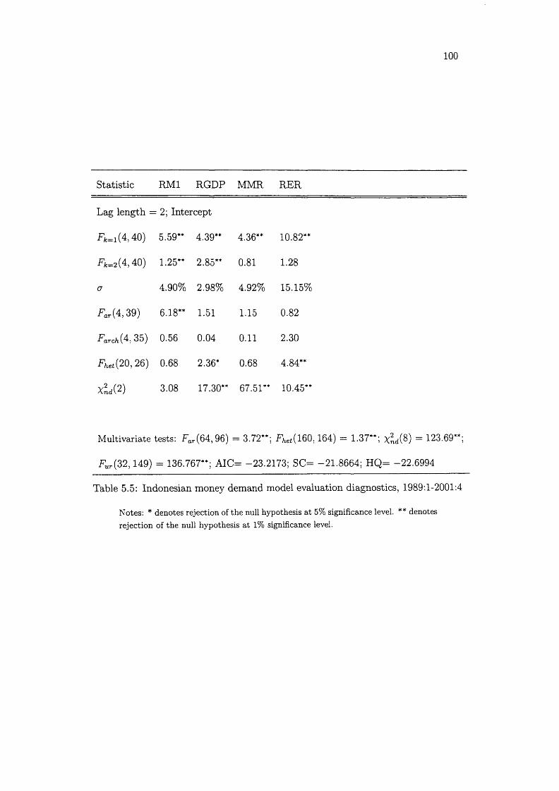
100
Statistic RM1 RGDP MMR RER
Lag length == 2; Intercept
iW 4 ,4 0 ) 5.59** 4.39** 4.36** 10.82**
i W M O ) 1.25** 2.85** 0.81 1.28
o 4.90% 2.98% 4.92% 15.15%
Far( 4,39) 6.18** 1.51 1.15 0.82
Farchi.^1 35) 0.56 0.04 0.11 2.30
Fhet(20,26) 0.68 2.36* 0.68 4.84**
Xnd( 2) 3.08 17.30** 67.51** 10.45**
Multivariate tests: Fai.(64,96) == 3.72**; Fhet( 160,164) = 1.37**; x l M = 123.69**;
Fur(32,149) = 136.767**; AID= -23.2173; SC= -21.8664; H Q = -22.6994
Table 5.5: Indonesian money demand model evaluation diagnostics, 1989:1-2001:4
Notes: * denotes rejection of the null hypothesis at 5% significance level. ** denotesrejection of the null hypothesis at 1% significance level.
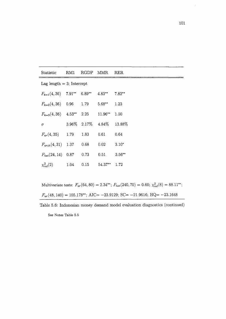
101
Statistic RM1 RGDP MMR RER
Lag length == 3; Intercept
F k= i(4,36) 7 .9 1 ** 6.89** 4.83** 7.82**
F k=2(4 , 36) 0.96 1.79 5.68** 1.23
^ = 3(4 , 36) 4.53** 2.25 11.96** 1.50
a 3.96% 2.17% 4.84% 13.88%
F ar(4 , 35) 1.79 1.83 0.61 0.64
Farchi^i 31) 1.37 0.68 0.02 3.10*
F het{ 24,14) 0.87 0.73 0.51 3.56**
xL (2) 1.04 0.15 54.37** 1.72
Multivariate tests: F a7 'o> 00 o = 2.34**; F h eti240,70) = 0.60; x l M = 88.11**;
Eur(48 ,140) = 105.178**; AIC = -23.9129; SC= -21.9616; HQ= -23.1648
Table 5.6: Indonesian money demand model evaluation diagnostics (continued)
See Notes Table 5.5
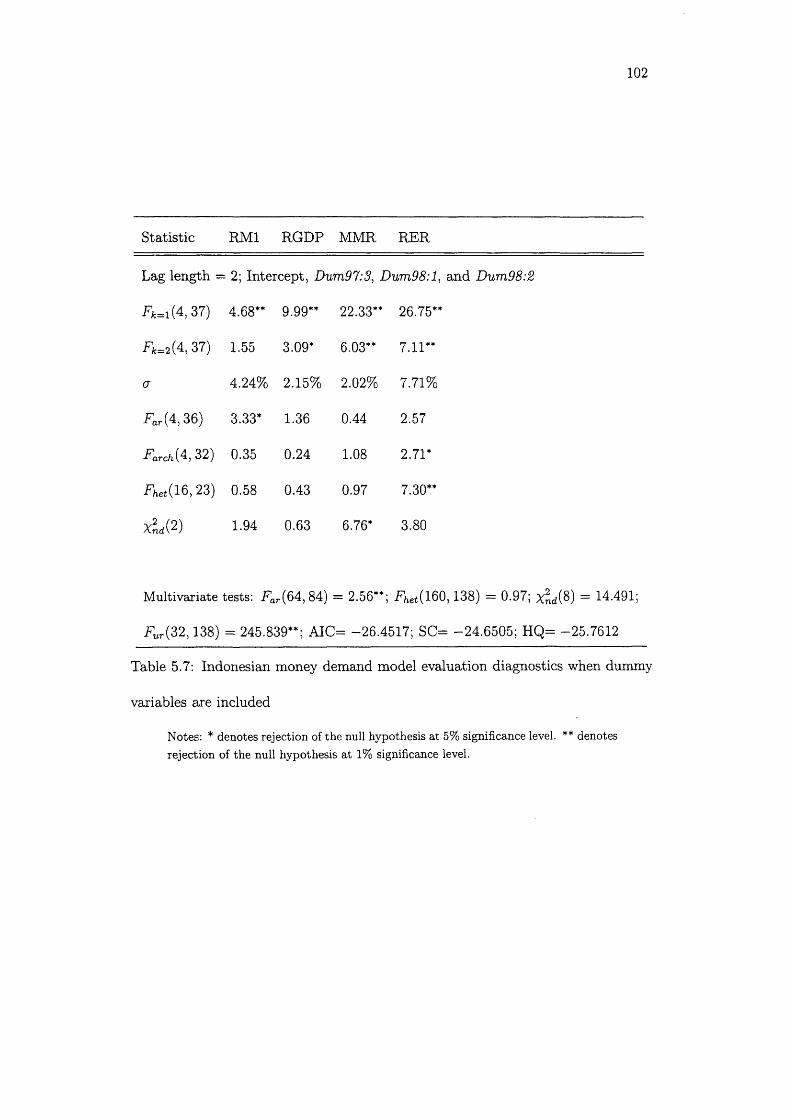
102
Statistic EM I RGDP MMR RER
Lag length == 2; Intercept, Dum97:3, D um 98:l, and Dum98:2
a = i ( 4,37) 4.68** 9.99** 22.33** 26.75**
4,37) 1.55 3.09* 6.03** 7.11**
<7 4.24% 2.15% 2.02% 7.71%
Far (4, 36) 3.33* 1.36 0.44 2.57
Farch(4, 32) 0.35 0.24 1.08 2.71*
^ ,( 1 6 ,2 3 ) 0.58 0.43 0.97 7.30**
Xnrf(2) 1.94 0.63 6.76* 3.80
Multivariate tests: Fai
00CO = 2.56**; Fhet( im , 138) = 0.97; X^ (8 ) = 14.491;
Fur (32 ,138) = 245.839**; AIC = -26.4517; SC= -24.6505; HQ= -25.7612
Table 5.7: Indonesian money demand model evaluation diagnostics when dummy
variables are included
Notes: * denotes rejection of the null hypothesis at 5% significance level. ** denotesrejection of the null hypothesis at 1% significance level.

103
the hypotheses: that the i-period lag (Fk=i) is zero; that there is no serial cor
relation (Far, against fourth-order autoregression); that there is no autoregressive
conditional heteroskedasticity (ARCH) (.Farch , against fourth order); that there
is no heteroskedasticity (Fhet)\ and lastly a x 2-test for normality (x2d)- Analogous
system (vector) tests are also reported, with the last test Fur representing the test
against the significance of the regressors in D t.
Density
Density
Figure 5.1: Residuals (scaled) and residual densities for RM1, RGDP, MMR, and
RER, lag length=2
The results indicate that the second period lag is significant in at least two of
the equations in the model. The null hypothesis of no serial correlation is rejected
in the univariate case for the real money supply (cf. the Far statistics against
fourth-order autoregression) and for the system as a whole. There is also some
evidence th a t the residuals from the real output, interest rate and exchange rate
equations are non-normally distributed. The impact of the out her observations is

104
seen more clearly in Figure 5.1. The residual plots indicate that the outlier problem
is largely associated with the third quarter of 1997 and the first and second quarters
of 1998.
Figure 5.2: Residuals (scaled) and residuals densities for RM1, RGDP, MMR, and
RER, lag length=2, including Dum97:3, Dum98:l, Dum98:2
Increasing the lag length to k = 3 produces the results in Table 5.6; the
additional lags are only significant in the real money and interest rate equations,
serial correlation is no longer a problem, although the test for ARCH is significant
for the exchange rate equation. Non-normal residuals are now only a problem
in the equation determining MMR. However, the null hypothesis of normality in
the system as a whole is rejected. In contrast, keeping k = 2 and including three
dummy variables (labelled Dum97:3, Dum98:l, and Dum98:2, taking the value of 1
for each of these quarters) improves the stochastic properties of the model without
the risk of overparametrising. The results axe shown in Table 5.7. Although

the residuals from the interest rate equation are still non-normally distributed,
normality is no longer rejected in the other equations and in the system as a
whole. This is seen more clearly in Figure 5.2 which gives the plots of the residuals
and residual densities when the three dummy variables are included. This points
to a potential trade-off in terms of setting the value of k and introducing 7(0)
variables into D t.
Figure 5.3: Plots of the vectors
Alternatively, if real output, interest rate, and exchange rate prove to be weakly
exogenous, then non-normality is less of a problem since one can condition on the
weakly exogenous variables and improve the stochastic properties of the model.3
It would therefore be appropriate to condition on these three variables instead of
adding extra dummy variables.
In what follows, the Johansen reduced rank approach is applied to the model
3 The test for weak exogeneity of the above variables is conducted at a later stage.

106
1995
1995
Figure 5.4: Plots of the vectors, corrected for short-run dynamics
H o'.r Ai Amax adj. c.v. adj. Atrace adj. c.v. adj.
0 0.466 32.67* 27.65* 27.42 32.35 71.76* 60.72** 48.88 57.67
1 0.412 27.67* 23.42* 21.12 24.92 39.08* 33.07* 31.54 37.21
2 0.149 8.41 7.12 14.88 17.55 11.41 9.66 17.86 21.07
3 0.059 3.00 2.54 8.07 9.52 3.00 2.54 8.07 9.52
Table 5.8: Test of the cointegration rank of the Indonesian money demand model,
unrestricted intercepts and no trends, 1989:1-2001:4
Notes:* and ** denote rejection of the null hypothesis at 1% and 5% significancelevel respectively. Critical values are from Table 6c in Pesaran et al. (2000).

107
H o - r rest. int.-no trends unrest, int.-no trends unrest, int.-rest, trends
0 114.26 71.76 105.11
1 65.20 39.08 54.63
2 34.42 11.41* 25.61
3 7.47 3.00 7.88
Table 5.9: Determining cointegration rank and the model for the deterministic
components using the trace test, Indonesian money demand data, 1989:1-2001:4
Notes: * Cannot reject the null hypothesis at the 5% significance level. Critical values are from Pesaran et al. (2000).
RM1 RGDP MMR RER
"Co 1 o o o 0.793 -0.504 0.290
- (11.36) (-3 .53) (6.38)
a' 0.312 -0.136 -0.040 0.228
(3.57) (-2.69) (-0.40) (0.83)
Table 5.10: Normalised cointegration coefficients of the Indonesian money demand
model, 1989:1-2001:4
Notes: Model with unrestricted intercepts and no trends. Based on 1 cointegration vector, t-values in parenthesis.

108
X2(3) = 7.40, p-value = 0.059
RM1 RGDP MMR R ER
& - 1.000 0.793 -0 .386 0.299
a! 0.524 0.000 0.000 0.000
(5.92) (0.00) (0.00) (0.00)
Table 5.11: Test for weak exogeneity of RGDP, MMR, and RER
Notes: Based on LR test of restrictions on a . t-values in parenthesis.
discussed above (with intercept, no dummy variables, and k = 2). Firstly, in
discussing the formulation of the dynamic model, the questions of whether an
intercept and trend should enter the short- and/or long-run model needs to be
considered. Following Johansen (1992c), the joint hypothesis of both the rank
order and the deterministic components is tested based on the so-called Pantula
principle.4 The results from estimating the various alternatives and then applying
the Pantula principle are presented in Table 5.9. The first time the null is not
rejected is indicated by the *. Thus, one can accept th a t there are at most two
cointegrating vectors and there are deterministic trends in the levels of the data.
The results of the trace and maximum eigenvalue tests are detailed in Table 5.8.
However, Reimers (1992) inter alia argues th a t in small samples the Johansen
procedure over-rejects when the null is true. Reimers suggests taking account of the
4 That is, all three models are estimated (restricted intercepts-no trends, unrestricted intercepts-no trends, and unrestricted intercepts-restricted trends). The results are presented from the most restrictive alternative (r = 0 and restricted intercepts-no trends) through to the least restrictive alternative (r = 3 and unrestricted intercepts-restricted trends). The test procedure is then to move through from the least restrictive model and at each stage to compare the trace statistic to its critical value and only stop the first time the null hypothesis is not rejected.

109
number of parameters to be estimated in the model and making an adjustment
for degrees of freedom to obtain satisfactory size properties in finite samples.5
In contrast, Cheung and Lai (1993) suggest making finite-sample corrections by
adjusting th e critical values and not the tests statistics.6 Table 5.8 shows that using
adjusted critical values/test statistics produces results similar to those obtained
when no adjustm ent is made.
These results can be seen more clearly in Figure 5.3 which plots the four
relations (associated with the four rows in p i ) . The first two vectors correspond
to the m ost stationary relations in the model, but there is evidence that both
relationships are upward trending. The other two vectors are clearly nonstationary.
The plots in Figure 5.4 confirm these findings while presenting a different version
of the sam e relations, with all the short-run dynamics removed.7
Doornik and Hendry (2001) point out that it is still unclear which correction
should be preferred.8 Juselius (1995) suggests instead looking at the eigenvalues
(i.e., the roots) of the companion matrix. There are 8 roots of the companion ma
trix. The moduli of the three largest roots are 0.989, 0.896 and 0.896, respectively,
5 This is accomplished by multiplying the tests statistics by a factor (T — n k ) /T where T is the number of observations, n is the number of variables in the VAR system and k is the lag length of the VAR.
6 In addition, Cheung and Lai (1993) find that the trace test is more robust to non-normality in the residuals than the maximum eigenvalue test. Skewness in the residuals is found to have a statistically significant effect on the test sizes of both the Johansen tests, but less so for the trace test. The latter also appears to be more robust to excess kurtosis (in the residuals) than the maximum eigenvalue test.
7 See Doornik and Hendry (2001) for further details.8 An alternative to making finite-sample corrections would be to simulate the exact distribu
tion based on the d.g.p. underlying the model being considered, using bootstrap methods, but this is not without problems. The results in Harris and Judge (1998) suggest that the bootstrap test statistic has poor size properties.
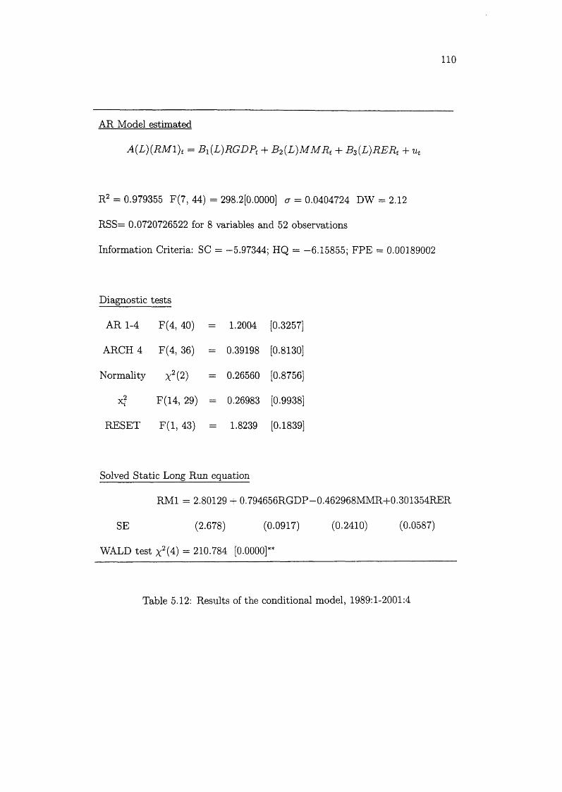
110
AR Model estimated
A {L ){R M l)t = B ^ R G D P t + B 2(L )M M R t + B 3(L )R E R t + ut
R2 = 0.979355 F(7, 44) = 298.2[0.0000] a = 0.0404724 DW = 2.12
RSS= 0.0720726522 for 8 variables and 52 observations
Information Criteria: SC = -5.97344; HQ = —6.15855; FPE = 0.00189002
Diagnostic tests
AR 1-4 F(4, 40) - 1.2004 [0.3257]
ARCH 4 F(4, 36) = 0.39198 [0.8130]
Normality X2(2) = 0.26560 [0.8756]
x? F(14, 29) - 0.26983 [0.9938]
RESET F (l, 43) = 1.8239 [0.1839]
Solved Static Long Run equation
RM1 = 2.80129 + 0.794656RGDP
SE (2.678) (0.0917)
WALD test x 2(4) = 210.784 [0.0000]"*
—0.462968MMR+0.301354RER
(0.2410) (0.0587)
Table 5.12: Results of the conditional model, 1989:1-2001:4

Test on the significance of each variable
variable F(num, denom) Value Probability
RM1 F(l,44)= 49.919 r --------V*
Constant F (l,44)= 0.94228 [0.3370]
RGDP F(2,44)= 7.8034 [0.0013]**
MMR F(2,44)= 4.3591 [0.0187]*
RER F(2,44)= 20.116 [0.0000]**
Test on the significance of each lag
Lag 1 F(4,44)= 49.902 [0.0000]**
COMFAC WALD test statistic table COMFAC F(3, 44)= 9.99203 [0.0000]*
Order Cumulative tests Incremental tests
1 *2(3) = 29.976 [0.0000]** x 2(3) = 29.976 [0.0000]**
Table 5.13: Tests of significance of each variable/lag and COMFAC tests
indicating tha t all roots are inside the unit circle with the three largest close to
unity. This suggests tha t ( n - r ) = 3. Thus it is possible to accept tha t there is one
cointegration vector (and deterministic trends in the levels of the data), which is
consistent with our theoretical prior on the existence of a long-run money demand
function. The estimates of a and (3 with their i-statistics (assuming r = 1 and
normalising on R M l t) are presented in Table 5.10.
Since one cointegration relation is identified, the weak exogeneity test are eval-
C9D

112
uated under the assumption of rank one. The null hypothesis tha t RG D Pt , M M R t
and R E R t are weakly exogenous is tested, thus imposing three row restrictions on
a . The results are presented in Table 5.11. Weak exogeneity of all three vari
ables is not rejected at the 5% significance level. This indicates th a t it is valid to
condition on these variables and use a single equation estimator of the cointegra
tion vector. Furthermore, comparison of the Johansen multivariate estimator of
P'fvii = [1-0, 0.793, —0.504, 0.29] with the single equation estimator of 0 part = [1.0,
0.794, —0.462, 0.301] reported in Table 5.12 shows th a t the two approaches are
equivalent.
The Wald test decisively rejects the null hypothesis th a t all the long-run coef
ficients (except the intercept term) are zero. The income elasticity is close to unity
and the interest and real exchange rates both have coefficients which are quite well
determined, correctly signed and highly significant. The income and interest rate
response lies in the range found in the inventory-theoretic model of Miller and Orr
(1966, 1968), and therefore could represent a structural response. Formal checks
on whether the model is data coherent are provided by testing for residual auto
correlation (fourth-order), ARCH (fourth order), normality and functional form
misspecification. The results reveal no problems.
Next, we tu rn to the analysis of the lag structure. The results are shown
in Table 5.13: every F -test is significant.9 The F -test on the significance of the
first-order lag shows tha t this lag m atters greatly. Finally, tests of common factors
9 The F-tests axe tests of the joint significance of the associated variables, with all their lags, and provide tests for deleting each variable completely from the model.

113
(COMFAC) in the lag polynomials also reported in Table 5.13 reject the hypothesis
of four common factors (see Doornik and Hendry (2001) for an interpretation).
Thus, we tentatively conclude that this model provides a cointegrated and data
congruent representation of Indonesian money demand.
The model is next used to test whether there has been a shift in the long-run
relationship amongst the variables in the money demand function. In order to
test this proposition, the methodology of Gregory and Hansen (1996) described in
the previous section is followed. The results are shown in Table 5.14. For all the
statistics the maximum lag length is chosen using the formula reported in Schwert
(1989, p. 151): kmax = int(12(T/100)ly/4. The selection of lag is based on the
significant t method but other procedures based on information criteria (e.g., AIC,
SC, HQ) have given identical results.
The conventional ADF test rejects the null hypothesis of no cointegration at
the 5% significance level both in the model with intercept and in the model with
intercept and trend. The ADF* tests which allow for a level shift (the C and C /T
tests) also reject the null hypothesis at the 10% significance level with structural
breaks occurring in the last quarter of 1997 and in the second quarter of 1991,
respectively. These results can be seen more clearly in Figure 5.5 which plots the
ADF* for level shift (C), level shift with trend (C /T ) and regime shift (C/S).
Turning now to the P P statistics, the Zt* test which allows for a level shift
is the only test which rejects the null hypothesis. Again, the structural break is
identified with the last quarter of 1997.

114
Test statistics Break point
ADF*
C -5.17** (0.71)
C /T -5.34** (0.19)
C/S -5 .71 (0.78)
Rc -5.20** (0.71)
C /T -5 .24 (0.23)
C/S -5 .68 (0.75)
c -34.47 (0.71)
C /T -35.20 (0.23)
C/S -38.93 (0.75)
ADF
C -4.33* -
C /T -4.26* -
Table 5.14: Tests of cointegration with regime shifts
Note: * and ** denotes rejection of the null hypothesis of no cointegration at the5% and 10% significance level respectively. Critical values for ADF*, Z*, and Z*are from Table 1 in Gregory and Hansen (1996).

115
1995 19971996 1999 2000
Figure 5.5: Regime shifts with ADF*, Indonesian money demand, 1989:1-2001:4
5.4 Conclusions
Using a residual-based cointegration test with regime shift we find supporting
evidence of a level shift (with trend) occurring in the second quarter of 1991 and
coinciding with the Sumarlin shock. We also find evidence of a level shift in the
money demand function occurring in the last quarter of 1997. This result corrob
orates the finding of the previous chapter: the timing of this break both in the
univariate and multivariate contexts can be linked to the crisis and a government
intervention in the money market for which the Sumarlin shock of 1991 is the
precedent. These results suggest that the decision by the Indonesian monetary
authorities in the aftermath of the crisis to move away from monetary gowth tar
geting towards inflation targeting may be well-placed. In effect, one of the main
advantages of inflation targeting over monetary targeting is that velocity shocks
are irrelevant because the monetary policy strategy no longer relies on a stable
money demand function (Mishkin, 1999).

116
Furthermore, the examination of the exogeneity property of the conditioning
variables in the long-run money demand function has revealed th a t both the in
terest and real exchange rates variables are weakly exogenous. The result for the
exchange rate is not surprising because for the sample period up to the third quar
ter of 1997 it has been more or less fixed (i.e. allowed to fluctuate within an
intervention band widened several times). Hence, the exchange rate was not deter
mined endogenously within the system. The fact th a t the interest rate is weakly
exogenous indicates tha t it might not be possible to recoup any type of interest
rate policy such as a Taylor rule.
The above findings lend support to the conventional Mundell-Fleming model
which postulates that the trinity of open capital markets, pegged exchange rate
regime and monetary policy autonomy is inconsistent. Since monetary policy is
primarily directed to maintaining the peg between the Rupiah and the US dollar,
monetary policy effects are potentially undermined and immobilised.

117
Appendix: D ata definitions and sources
For each series the sample period is 1983:1-2001:4. The series are all seasonally
adjusted (with the exception of the interest rate and real exchange rate series).10
The source is the IMFs International Financial Statistics (except where a different
source is mentioned).
(1) R M 1, and R M 2 are the natural logarithms of the M l and M2 definitions
of the money stock (in billion rupiahs), each deflated by the consumer price index
(1995=100). Source: Bank Indonesia (unpublished).
(2) RG D P is the natural logarithm of the Indonesian gross domestic product
at 1995 m arket prices (in billion rupiahs). Source: Bank Indonesia (unpublished).
(3) M M R is the nominal money market rate (in level).
(4) IN F is the inflation rate, computed as the change in the consumer price
index (1995=100).
(5) U STBR is the nominal 3-months US T-bill rate (in level).
(6) R E R is the Indonesian exchange rate in real terms, computed as:
\i(wpit)-i(wprt) + i(E t)}
where E t is the nominal Rupiah exchange rate defined as the foreign price of
domestic currency (indirect quotation, a rise represents an Indonesian currency
appreciation). Source: IMFs International Financial Statistics. W P It is the do
mestic wholesale price index (1995=100). W P I is a weighted average of foreign
10 See chapter 4, Appendix A.

wholesale price indices (1995=100) computed as:
mrW P l* = Y jw ^ W P Ijt ,
j - 1
where w'j are fixed weights and m r = 4.11
11 See chapter 4, Appendix A.

CHAPTER 6
ARDL APPROACH TO MODELLING INDONESIAN MONEY DEMAND
WITH FINANCIAL LIBERALISATION
6.1 Introduction
Traditional specifications of money demand applied to countries under financial
liberalisation often yield parameter estimates tha t are not economically plausible,
are subject to highly autocorrelated errors (Courakis, 1978), and frequently re
sult in persistent overprediction of money demand, the so-called missing money
episodes (Goldfeld, 1973; 1976). Inspection of the da ta reveals shifts, or continuing
movements in holdings of money balances tha t are unrelated to the behaviour of
the explanatory variables tha t appear most commonly in the literature. These
shifts can be attributed, at least in part, to financial market developments. These
developments cannot be considered as part of a stationary error term since their
effect on money demand is permanent (Arrau et al., 1995). It then follows that,
for countries under financial liberalisation , money demand functions tha t do not
explicitly control for this process are likely to be misspecified.
In principle, financial liberalisation can be captured in the money demand
function in various ways: by including dummy variables (Friedman and Schwartz,
1982), a deterministic trend (Moore et al., 1990; Arrau et al., 1995; Dekle and
Pradhan, 1999), institutionally-related variables (Bordo and Jonung, 1981; 1987;

120
1990; Siklos, 1993; Klovland, 1983; Akhtar, 1983)1, or by adjusting monetary
indices (Binner et al, 2004).
In this chapter, the empirical implications of financial liberalisation are ex
plored by introducing a deterministic trend as an additional explanatory variable
in the money demand function for Indonesia. As already argued in chapters 4 and
5, standard cointegration procedures, which have been widely used to estimate the
long-run demand for money, may not be appropriate when applied to countries
under financial liberalisation. This phenomenon is widely associated in the empir
ical literature with structural change. Instead, the procedure carried out in this
chapter—the ARDL modelling approach of Pesaran et al (2001)—is based on as
ymptotic critical value bounds for the Wald or F-statistics. It follows that one can
investigate the existence of the long-run money demand function for Indonesia, in
the presence of financial liberalisation, without the need to know if the variables
included in the money demand function are integrated, stationary, or mutually
cointegrated.
A similar strategy is used to estimate import demand functions for Cyprus
(Pattichis, 1999) and Korea (Mah, 2000). Ghatak and Siddiki (2001) also use this
approach to estimate virtual exchange rates in India. Tang (2001; 2002) use the
procedure to model inflation behaviour and the demand for M3 in Malaysia.2
1 Examples of such institutionally-related variables are bank offices per head of population, the proportion of the labor force employed outside of agriculture, the ratio of currency to total money stock, the ratio of non-bank to bank financial assets, etc...
2 These authors have used earlier unpublished versions of Pesaran et a l (2001) entitled: "Bounds Testing Approaches to the Analysis of Level Relationships", DAE Working Paper Series No. 9622 (1996) and No. 9907 (1999), Cambridge University, Department of Applied Economics.

121
The rest of the chapter is organised as follows. Section 6.2 discusses the ARDL
methodology. The description of the d a ta and the empirical results are presented
in Section 6.3. Section 6.4 offers some concluding remarks.
6.2 Methodology
The econometric specification used in this chapter is similar to the one used in
the previous chapter. Real money dem and is a function of a scale variable (e.g.,
the level of real income), and an opportunity cost variable (e.g., the rate of interest
on an alternative asset). The availability of foreign currency assets for investment
implies th a t the variety of assets available for portfolio diversification is wider
(Chowdury, 1997). The direct currency substitution literature, which suggests
portfolio shifts between domestic and foreign money, focuses on the exchange rate
variable, whereas the capital mobility literature focuses on the foreign interest rate
variable (Cuddington, 1983; Leventakis, 1993, Tan, 1997). We include a foreign
interest rate variable to obtain the open-economy version of the money demand
function.
As argued in Lieberman (1977, 1979), measuring the impact of technological
change on money demand is a difficult exercise. Ideally, one would like to model
explicitly each source of improvement in cash management. Unfortunately, innova
tions in cash management include many new activities, instruments, institutions,
and practices for which data are often sparse or non-existent. Even if it were
feasible, modelling each source of innovation would quickly exhaust the degree of
freedom available. Conversely, omitting any measure of technological change is

122
hardly costless. If technological change is ignored, the coefficients estimates will
be biased. As a result, even crude proxies for the om itted variable, technological
change, should be considered.
A crude proxy for technological change which is commonly used elsewhere in
the literature is a deterministic trend. The inclusion of a trend in the estimation
merely assumes th a t the implementation of new technologies or practices reduces
money dem and smoothly over time. Although the introduction of new technologies
or cash management methods may be discrete or lumpy rather than continuous,
the im plem entation of such methods throughout the economy will be distributed
with a lag, thereby smoothing out the impact on money balances. A deterministic
trend would measure the mean rate at which new cash management techniques
have an effect on money balances, assuming technological change is exogenous to
the financial sector (Lieberman, 1979).
Since money dem and is not directly observable, it is assumed tha t the money
market is always in equilibrium and th a t the money supply is exogenous. Thus,
one can identify the money demand function described above and use the quantity
of money to measure the demand for money.
Following the modelling approach developed in Pesaran, Shin and Smith (2001)
(PSS hereafter) the section starts from the maintained assumption th a t the time
series properties of the variables included in the money demand function can be
well approxim ated by a log-linear VAR(p) model. Let:

123
z t = [mu Vu Rt, - R ? ] ' = [ m t , x t ] ' ( 6 . 1 )
where m t is real money balances (in logarithms), yt is real income (in loga
rithm s), R t is the nominal domestic interest rate (in levels), and is the foreign
interest ra te (in levels).
The conditional (partial) model can be written as:
p - i
A m t = c0 + cit + 7rmrnm t_i 4- 7r + w ' A x * + ut (6.2)i = 1
where Co is an intercept, t is a deterministic trend, and ut ~ IID (0 ,a2).
Under the assumption th a t lagged real money demand, m t- 1 , does not enter the
sub-VAR model for Xt, for equation (6.2) the above real money demand function
is identified and estim ated consistently by the OLS. PSS developed bounds tests
to test th e existence of a long-run relationship between the levels of m t and Xt,
t = 1 ,2 ,.... More specifically, the approach consists in testing for the absence of
any long-run relationship between m t and x t , t = 1 ,2 ,...; tha t is, the exclusion of
the lagged level variables m t- 1 and xt- i h1 (6-2). Hence, the null hypotheses are
given by:
tT7Tmm . _ — f) T J ^ m x . x . — — fV-CZq . 71 m m — U , 1J.Q . 71 m x .m — u
and th e alternative hypotheses by:
H*mrn : 7Tmm 7̂ 0, H f mx x : 7 rm x .m ^ O'.

124
Since the asymptotic distributions of the F- and t- statistics are non-standard
under the null hypothesis, irrespective of whether the forcing variables {x^} are
1(0) or 1(1), PSS provide two sets of critical values for these statistics covering
various specifications of the deterministic terms; one set assuming tha t the forcing
variables {xt} are 7(0) and the other assuming th a t {xt} are 1(1). These two sets
provide lower and upper critical value bounds covering all possible classifications
of {xt} into 1(0), 1(1) and mutually cointegrated processes. If the computed Wald
or F- statistics fall outside the critical value bounds, a conclusive decision results
without needing to know the cointegration rank r of the {xt} process. If, however,
the Wald or F- statistics fall within these bounds, inference would be inconclusive,
and knowledge of the cointegration rank r of the forcing variables {xt} is necessary
to proceed further.
6.3 Empirical results
This study uses quarterly data from 1983:1 to 2000:4. The logarithm of the
monetary aggregate M2 (broad money) is used to proxy m. In the Indonesian
context, Dekle and P radhan (1999) have argued th a t the behaviour of broad money
velocity seems to be better captured by a deterministic trend (the chosen proxy for
financial liberalisation ) than the behaviour of narrow money velocity. Since the
model requires money demand in real terms, the consumer price index (with the
base 1993) is used as a deflator. The logarithm of the real gross domestic product
is used as a proxy for y. The domestic interest rate, R , is proxied by the money
m arket ra te (a typical value is 0.10). R*, the foreign interest rate, is proxied by
125
the 3-months US T-Bill rate (a typical value is 0.10).3
Two impulse dummy variables are entered in the short-run p a rt of the model
to dummy out two outliers in the data. These dummy variables are defined by
Dum90:4t = 1 for the fourth quarter of 1990 and zero elsewhere,
Dum98:2t = 1 for the second quarter of 1998 and zero elsewhere.
It is w orth mentioning tha t the asymptotic theory on which the bounds test is
developed is not affected by the inclusion of such one-off dummy variables. The
results of the estimation of (6.2) without including the two dummy variables are
reported in Table 6.4. The estimated coefficients axe very close to those obtained
when the dummy variables are included in the model. However, the Bera-Jarque
test suggests a problem of non-normality, giving further support to the inclusion
of the dummy variables to dummy out the outliers.
To determine the appropriate lag length, p, and whether it is im portant to add
the proxy for financial liberalisation, the deterministic trend, to the income and
interest ra te variables, model (6.2) was estimated by the OLS w ith and without
a deterministic trend, for p = 1,2. Unfortunately, the size of the sample does not
allow to estim ate (6.2) for higher lag lengths as the degree of freedom needs to
be saved. First-lagged changes of the income and domestic interest rate variables,
Apt_i and A R t- i , were found not significant (either singly or jointly) when a
determ inistic linear trend is included in the regression. First-lagged change of
3 Data on nominal M2 are from Bank Indonesia (unpublished). Data on real gross domestic product (at constant prices 1993) are from Biro Pusat Statistik (BPS, Central Bureau of Statistics, unpublished). Data on the consumer price index, the money market rate and the US 3-months treasury bill rate are from the IMF’s International Financial Statistics (IFS).

126
the income variable and the first-difference of the foreign interest rate variable.
A y t- i and AF£, were also found not significant (either singly or jointly) when the
regression did not contain a deterministic trend. Therefore, in both cases, for p =
2, parsimonious versions of (6.2) were re-estimated to avoid overparameterisation.
Table 6.1 gives the Akaike’s Information, Schwarz’s Bayesian Criteria and the
Lagrange multiplier (LM) statistics for testing the hypothesis of serial correlation
of order 1 and 4. These are denoted by (1) and (4), respectively. The AIC suggests
the lag order, p, to be 1 when the model contains a trend and 2 when it does not.
The SC criterion, on the contrary, suggests p to be only 1, irrespective of whether a
determ inistic trend is included in the model or not. The Xsc (4) statistic suggests
to select p to be either 1 or 2 if the model includes a deterministic trend, but only
2 if the model does not.
Table 6.2 gives the values of the F - and t-statistics for testing the existence
of a long-run money demand function under three different cases depending on
whether the model contains a linear trend and whether the trend coefficients are
restricted. The F- and t-statistics in Table 6.2 are compared with the critical value
bounds provided in Tables C l and C2 in PSS.
F irst, consider the bounds F-test. For the model with a deterministic trend,
Fv is the standard F -statistic for testing the restrictions 7zmm = 0 and 7rmx.x = 0,
while F /v is the standard F-statistic for testing 7rmm = 0, 7rmx.x = 0, and c\ = 0
in (6.2). As argued in Pesaran, Shin and Smith (2000), the statistic FIV, which
sets the trend coefficient to zero under the null of no long-run level relationship,
127
is more appropriate than Fy, which does not impose this restriction. The critical
value bounds for the statistics Fiy and Fy are given in Tables C l.iv and Cl.v,
respectively, in PSS. Since the model contains three regressors, the 95% critical
value bounds are (4.23, 5.29) and (4.01, 5.07) for F/y and Fy, respectively.
W hen a linear trend is included in the model, the test outcome critically de
pends on the choice of the lag order, p. For p = 1 (selected by the AIC), the
hypothesis th a t there exists no long-run money demand function is rejected at the
95% level, irrespective of whether the regressors are I (0) or 7(1). However, for p =
2, the statistics FIV and Fv are inconclusive. W hen the bounds F -test is applied
w ithout a linear trend, the 95% critical value bounds of the relevant test statistic,
the F /jj , are (3.23, 4.35). Irrespective of the lag order, the Fjjj statistic rejects
the null hypothesis of no long-run money demand function.
Table 6.2 also reports the results of the bounds F test to the money demand
functions. The two ^-statistics, ty and t j j j , are the Fratios of the OLS estimates
of TTmm in (6.2), w ith and without the deterministic trend, respectively. The
critical value bounds for these statistics are given in Tables C2.iii and C2.v in
PSS. These statistics show that the null hypothesis is not rejected for p = 2,
irrespective of whether the trend is included or not. However, for p = 1, the null
hypothesis is rejected w ith or without the trend. The test results therefore support
the existence of a long-run relationship when p = 1 and when the deterministic
trend is included in the model. This specification is in accord with the evidence
of the performance of the alternative models set out in Table 6.1.4 These results
4 It is likely that the results of the F m and t n i statistics reported in Table 6.3 for p = 1

128
W i th D e te rm in is tic T ren d s W ith o u t D e te rm in is tic T rends
V A IC SC Xsc (1) Xsc (4) A IC SC Xsc (1) Xsc (4)
1 116.04 105.86 4.59 6.41* 114.70 105.65 7.88 10.55
2 115.70 103.34 0.55* 1.30* 115.86 104.61 2.66** 4.24*
Table 6.1: Statistics for selecting the lag order of the Indonesian money demand
equation
Notes: p is the lag order of the conditional model (6.2), with zero restrictions on the coefficients of lagged changes in the y and R variables with deterministic trends and p = 2, and zero restrictions on the coefficients of lagged changes in the y and R* variables without deterministic trends and p = 2. A IC p = LLp — sp and SC p = LLp - ln(T), are the Akaike and Schwarz Information Criteria, where LLp is the maximised log-likelihood value of the model, p is the lag order, sp is the number of freely estimated coefficients, and T is the sample size. (1) and (4) are the LM statistics for testing the absence of residual serial correlations of order 1 and 4, respectively. The symbols f, and ff represent significance at 5% or less, and 10% or less, respectively.
129
show th a t the decision to include a deterministic trend in the model is not trivial.
Since the tren d captures financial liberalisation , it implies in turn that a long-
run money dem and relationship can only be obtained when the chosen proxy for
financial liberalisation is included.
The rem ainder of this chapter focuses on a money demand model which has a
lag order p = 1 and includes a deterministic trend. This specification yields the
following estim ated long-run money demand function:
m t = 1.526yt - 0.160#* - 1.021#* + 0.008* - 10.377 + vt (6.3)
where vt is th e equilibrium correction term.
As argued in Dekle and Pradhan (1997), financial liberalisation may change
the velocity of money, in principle, in either direction. Reforms that increase the
number of banks, and spur institutional and technological advances such as credit
cards, and electronic transfers of deposits or cash machines, can raise the velocity
of broad and narrow money, as these developments make it easier to convert money
into money substitu tes. However, recall tha t Bordo and Jonung (1990) hypothe
sised th a t in m any developing countries the velocity of broad money may decline
over tim e because of the increasing monetisation of the economy or financial deep
ening.5 Furtherm ore, there can be shifts between the various categories of money.
are affected by the existence of serial correlation in the residuals detected when the deterministic trend term is excluded from the model (see Table 6.1). In view of the importance of serially uncorrelated errors for the validity of the bounds tests, we conclude that the deterministic trend must be included in the model.
5 Bordo and Jonung suggest that the institutional and financial factors that systematically influence the demand for money in an economy over the entire course of its development are of two types. First, the process of monetisation, defined as the growth of the commercial banking
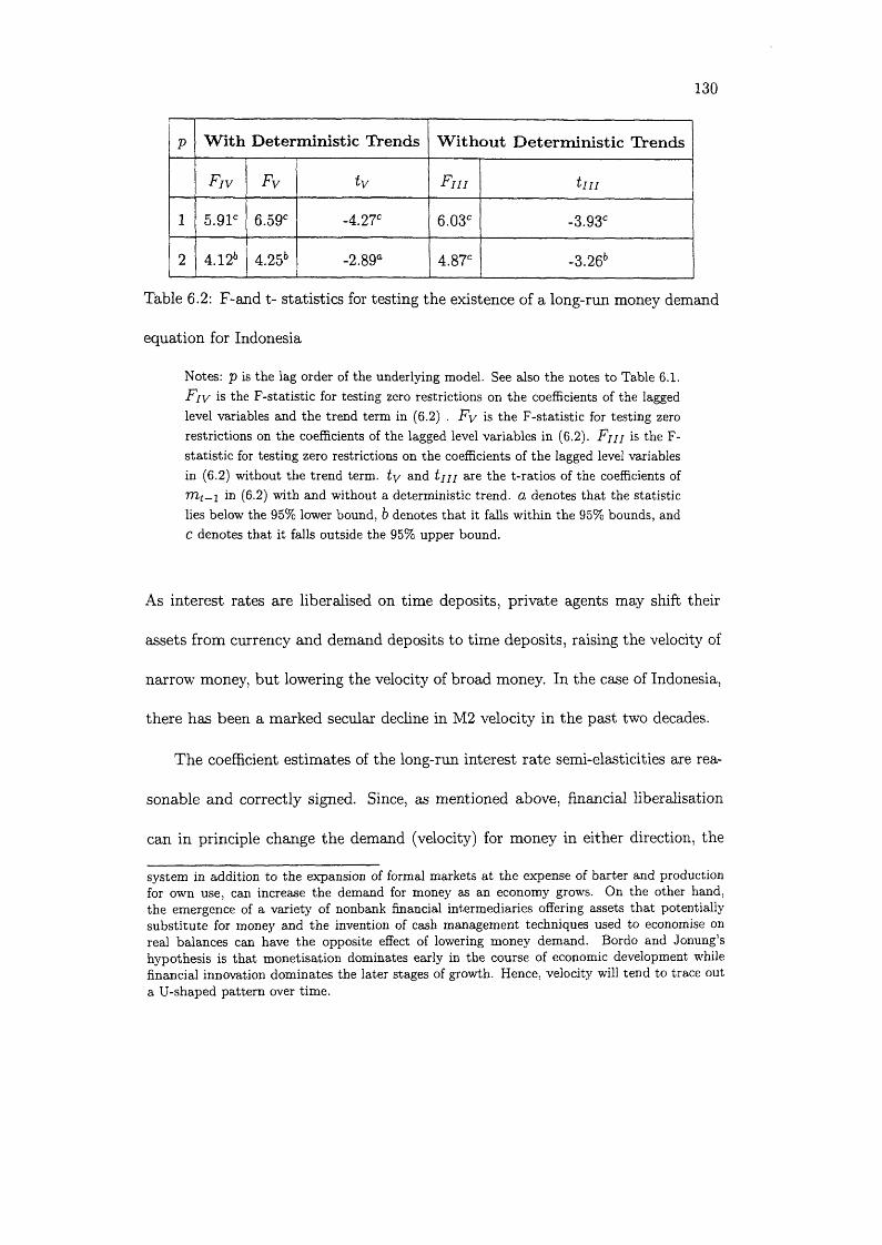
130
p W ith D e te rm in is tic T rends W ith o u t D e te rm in is tic T rends
F i v F y t y F i n t i n
1 5.9T 6.59° -4.27c 6.03c -3.93c
2 4.12b 4.25b -2.89a 4.87c -3.26b
Table 6.2: F-and t- statistics for testing the existence of a long-run money demand
equation for Indonesia
Notes: p is the lag order of the underlying model. See also the notes to Table 6.1.F i v is the F-statistic for testing zero restrictions on the coefficients of the lagged level variables and the trend term in (6.2) . F y is the F-statistic for testing zero restrictions on the coefficients of the lagged level variables in (6.2). F / / / is the F- statistic for testing zero restrictions on the coefficients of the lagged level variables in (6.2) without the trend term, t y and £ /// are the t-ratios of the coefficients of TTlt—i in (6.2) with and without a deterministic trend, a denotes that the statistic lies below the 95% lower bound, b denotes that it falls within the 95% bounds, and C denotes that it falls outside the 95% upper bound.
As interest rates are liberalised on time deposits, private agents may shift their
assets from currency and demand deposits to time deposits, raising the velocity of
narrow money, but lowering the velocity of broad money. In the case of Indonesia,
there has been a marked secular decline in M2 velocity in the past two decades.
The coefficient estimates of the long-run interest rate semi-elasticities are rea
sonable and correctly signed. Since, as mentioned above, financial liberalisation
can in principle change the demand (velocity) for money in either direction, the
system in addition to the expansion of formal markets at the expense of barter and production for own use, can increase the demand for money as an economy grows. On the other hand, the emergence of a variety of nonbank financial intermediaries offering assets that potentially substitute for money and the invention of cash management techniques used to economise on real balances can have the opposite effect of lowering money demand. Bordo and Jonung’s hypothesis is that monetisation dominates early in the course of economic development while financial innovation dominates the later stages of growth. Hence, velocity will tend to trace out a U-shaped pattern over time.

131
coefficient of the deterministic trend can have either a positive or negative sign.
In effect, the coefficient of the trend indicates a positive effect of financial liber
alisation on broad money demand of about 3.2 percent per year. In comparison,
Deckle and Pradhan (1999), using other measures of domestic and foreign interest
rates and annual data over 1974-1995, report a positive effect of 7.4 percent per
year.
The unrestricted error-correction regression associated with the above (level)
long-run relationship is reported in Table 6.3. All contemporaneous changes in the
income, and domestic and foreign interest rate variables are correctly signed and
statistically significant, further justifying the choice of p = 1. The equilibrium cor
rection coefficient is estimated to be -0.501, which is reasonably large and suggests
th a t the money demand process converges fairly rapidly towards its equilibrium
given by (6.3).
The regression fits reasonably well, and the plot of actual and fitted values
(see Figure 6.1) shows tha t the estimated model follows closely the path of the
actual variables and captures almost all the turning points. The model also passes
a number of diagnostic tests. The Bera-Jarque test for normality indicates tha t the
normality assumption appears to be consistent with the data. The Koenker-Bassett
test shows no evidence of heteroskedasticity. The Breusch-Godfrey Lagrange mul
tiplier (LM) test for serial correlation indicates no evidence of serial correlation up
to the fourth order. The model should not be given extra-credit for this result since
it was chosen specifically to meet this test.6 However, the regression fails Ramsey’s
6 The difference between the X sc (4) reported in Table 6.2 and the one reported in Table 6.1

132
Regressor Coefficient Standard Error p-value
rrit-i -.5013 N /A N /A
Vt-i .7651 N /A N /A
F t-1 -.0807 N /A N /A
F t-1 -.5121 N /A N /A
A yt .6835 .1474 .000
A R t -.1973 .0744 .010
A R i -3.1053 1.0183 .003
Intercept -5.2029 .9181 .000
t .0044 .0014 .003
D um 90A .1527 .0378 .000
Dum9S:2 .1923 .0418 .000
Adjusted-R2 = .5435, Standard Error of Regression = .0356, A IC — 130.91,
S C = 118.46, x 2SC (4) = 1.95[.743], x 2F F ( 1) = 9.04[.003], x 2iV(2) = 0.32[.851],
X 2 H { 1) = 0.18[.668]
Table 6.3: Unrestricted error correction model of the Indonesian money demand
equation
Notes: X2S 'C (4), X ^ F F i l ) . X2N ( 2), %2i / ( l ) are the Chi-squared statistics for tests of residual serial correlation, functional form misspecification, non-normal errors and heteroskedasticity, respectively.

133
RESET general test of misspecification at the 5% level. It may be the consequence
of the simple dynamic structure retained to save the degree of freedom. It could
also reflect some non-linear effects or asymmetries in the adjustment of real broad
money demand that the linear specification cannot take into account.
The CUSUM and CUSUMSQ tests, based on recursive estimation of the un
restricted error correction model, suggest that the regression coefficients are sta
tistically stable over the sample period.7 The plots of the cumulative sum and
cumulative sum of squares based on the recursive residuals are shown in Figures
6.2 and 6.3. They do not show evidence of statistically significant structural breaks.
Figure 6.1: Plot of actual and fitted values
is explained by the inclusion of the two impulse dummy variables in the regression.7 These tests do not require the possible break point in the data to be known a priori. The
CUSUM test detects systematic changes in the regression coefficients while the CUSUMSQ test is used to capture sudden departure from the constancy of regression coefficients. Note that the two impulse dummies are excluded from the model to allow the tests to be performed over the whole sample period.

134
Regressor Coefficient Standard Error p-value
m t - i -.4336 N/A N/A
Vt- i .6836 N/A N/A
Rt-1 -.0330 N/A N/A
D * 1 -.2782 N/A N/A
A yt .4374 .1764 .016
AR t -.1194 .0893 .186
a r ; -2.9904 1.2701 .022
Intercept -4.7373 1.1376 .000
t .0035 .0017 .044
Table 6.4: Unrestricted error correction model without impulse dummy variables
Adjusted-R2 = .2896, Standard Error of Regression = .0444, AIC = 116.04,
SC = 105.86, X2SC{4) = 6.41[.170], x 2F F ( l) = 6.91[.009], * 2iV(2) = 12.79[.002],
X 2 H { 1) = 0.02[.869]

135
Figure 6.2: Plot of cumulative sum of recursive residuals
Figure 6.3: Plot of cumulative sum of squares of recursive residuals
6.4 Conclusions
Previous research on financial liberalisation and money demand in Indone
sia is fairly limited. Using cointegration and estimating money demand (jointly
with a purchasing power parity equation) in the ASEAN-4 (Indonesia, Malaysia,
Singapore and Thailand), Dekle and Pradhan (1999) found tha t the money func
tion for Indonesia did not cointegrate when deterministic trend and step dummy
variables—controlling for financial liberalisation —were excluded. The determin
istic trend was found statistically significant but all three step dummy variables

136
were found insignificant.
Our findings support the inclusion in the money demand function for Indonesia
of the determ inistic trend as a crude proxy for financial liberalisation. In particular,
we show th a t the existence of the long-run money demand function can only be
firmly established when the trend is included in the model. Moreover, it is also
found to be statistically significant. This result is obtained, however, without the
need to include any exogenous step dummy variables. The model, however, does
not pass the misspecification test. This may be the consequence of the simple
dynamic structu re retained to save the degree of freedom. It could also reflect
some non-linear effects or asymmetries in the adjustment of real broad money
dem and th a t our linear specification cannot take into account.
From a policy perspective, the finding th a t Indonesian broad money was ex
trem ely sensitive to changes in the foreign (US) interest rate over the sample
period suggests th a t—while M2 appeared to be a reliable indicator of liquidity
conditions—controlling its growth was particularly difficult. Overall, the results
suggest th a t financial liberalisation does play an im portant role in determining
money dem and, and its fluctuations, in Indonesia. This study provides a robust
empirical basis for further research on the impact of financial liberalisation on
money dem and in countries which have experienced this phenomenon.

CHAPTER 7
CONCLUSION
In th is thesis, we have shown, through a battery of statistical tests, both in
univariate and multivariate contexts, th a t in effect, something structural seems to
have happened to money demand in Indonesia. There is supporting evidence of a
break in the money demand function occurring in the second quarter of 1991 and
coinciding with a major government intervention in the money market known as
the Sumarlin shock. We have also found evidence of a break, both in the univariate
series and the multivariate money demand relation occurring in the last quarter of
1997 coinciding with a deep recession and a government intervention in the money
market much similar to the earlier Sumarlin Shock of 1991.
The issue of distinguishing between stochastic processes with long memory and
those w ith short memory or stationarity tha t exhibit structural changes (chapter
4) is relevant because the current shocks will have temporary effects of greater
(integrated process) or lower duration (stationary process), and only occasional
events or shocks associated to structural breaks will have permanent effects on
the long-run level of the series. In effect, when stationary series with structural
breaks are observed, these few occasional shocks with long-duration effects would
produce certain persistence or symptoms of nonstationarity in the series. Since our
results were obtained under the maintained assumption tha t there was at most one
structu ral break, future research could give more attention to the issue of multiple

138
structura l breaks.
W hen estim ating breaks under common stochastic trends (chapter 5), it is
im portant to signal th a t conventional cointegration tests could yield misleading
results in the presence of structural breaks (Leybourne and Newbold, 2003). In
addition, the study of cointegration relations in the presence of structural breaks
is very complicated and even more, in case of more than two series, since the
instability or break could be in all or several cointegration coefficients, in the error
correction coefficient, in all long-run relations or in some of them, or in the short
run dynamics, and the breaks could happen contemporaneously in all the series or
not (Jimeno et al., 2006). Since our results were obtained under the maintained
hypothesis of cointegration they should be taken w ith some caution. Instability
in the number of cointegration relations or cointegration rank (probably due to
the presence of structural breaks in the cointegration relation) may have occurred.
Future research could apply the approaches of Hansen and Johansen (1999), Inoue
(1999), and Johansen et al. (2000) to test the cointegration rank allowing for
structural breaks.
Finally, we have shown how modelling financial liberalisation in the money
demand function as a deterministic drift process can result in an improvement
over the standard specifications in terms of yielding more constant and plausible
values for the param eters of the money demand function (chapter 6). In particular,
our findings support the existence of a stable long-run money demand function
for Indonesia which, unlike previous studies, does not rely on the inclusion of

139
statistically insignificant exogenous step dummy variables. This result is based on
a novel bu t robust econometric procedure which avoids pretesting of the order of
integration of the variables in the money demand function.
From a policy perspective, the findings tha t M l was sensitive to changes in
the exchange rate, and that the demand for narrow money may have undergone
a regime shift during the period under investigation suggest th a t a narrow money
growth target was not suitable. Similarly, the finding th a t the dem and for M2 was
stable bu t extremely sensitive to the foreign (US) interest rate suggests th a t—while
broad money appeared to be a reliable indicator of liquidity conditions throughout
the sample period—controlling its growth was particularly difficult.
More generally, our results support the notion th a t financial liberalisation
might have rendered the money supply endogenous, with respect to output. The
Indonesian central bank would have had difficulty in controlling the money supply
because even though it could manage to generate credit constraints in the In
donesian economy, Indonesian banks could easily borrow on international financial
markets, which undermined the effectiveness of monetary policy.
The above findings support the Mundell-Fleming type argument tha t the trin
ity of open capital markets, pegged exchange rate regime and m onetary policy is
inconsistent. Before the 1997 crisis, during periods of upswing in the economy,
rising aggregate demand was accompanied by both increased foreign borrowing
and the liquidation of SBI by sale to the central bank, both of which resulted
in increases in base money (given the quasi-fixed exchange rate regime). In such
140
context, controlling base money growth (and through it aggregate demand) was
difficult and required extremely high interest rates and/or dramatic contractions of
dom estic liquidity of the Sumarlin shock type. Most significantly, monetary policy
was im mobilised in the period before the decision to float the Rupiah in 1997.
Overall, our findings should foster more research at identifying the underlying
causes of m oney demand instability in Indonesia and other developing economies
w here sim ilar programmes of financial liberalisation have been implemented.

141
REFERENCES
Aghevli, B. B., M. S. Khan, P. R. Narvekar and K. Brock (1979). ‘Monetary Policy in Selected Asian Countries’, IMF Staff Paper No. 26, pp. 775-824.
Agrawal, P. (2001). ‘Interest Rates, Exchange Rates and Financial Deepening in Selected Asian Economies.’ A SE A N Economic Bulletin , vol. 18, pp. 83-93.
Akerlof, G. A. and R. D. Milbourne (1980). ‘The Short-Run Demand for Money.’ Economic Journal, vol. 90, pp. 885-900.
A khtar, M. A. (1983). ‘Financial Innovations and Their Implications for Monetary Policy: An International Perspective.’ B IS Economic Papers, vol. 9.
A lam syah, H., C. Joseph, J. Agung and D. Zulverdy (2001). ‘Towards Implementa tio n of Inflation Targeting in Indonesia.’ Bulletin of Indonesian Economic Studies , vol. 3, pp. 317-32.
Alogoskoufis, G. and R. Smith (1991). ‘On Error Correction Models: Specification, In terpretation, Estim ation.’ Journal of Economic Surveys, vol. 5, pp. 97-128.
A rrau , P., J. De Gregorio, C. M. Reinhart and P. Wickham (1995). ‘The Demand for Money in Developing Countries: Assessing the Role of Financial Innovation.’ Journal o f Development Economics, vol. 46, pp. 317-40.
A biad, A. and A. Mody (2005). ‘Financial Reform: W hat Shakes it? W hat Shapes i t? ’ American Economic Review, vol. 95, pp. 66-88.
B aba, Y., D. F. Hendry and R. M. Starr (1992). ‘The Demand for M l in the USA.’ Review of Economic Studies, vol. 59, pp. 25-61.
Bai, J. and P. Perron (1998). ‘Estimating and Testing Linear Models with Multiple S tructu ral Changes.’ Econometrica, vol. 66, pp. 47-78.
Bai, J. and P. Perron (2003). ‘Computation and Analysis of Multiple Structural C hange Models.’ Journal of Applied Econometrics, vol. 18, pp. 1-22.
B ank Indonesia (1995). Laporan Bulanan Ekonomi, Moneter dan Perbankan [Monthly Report on Economy, Monetary Affairs and Banking ], March.
B an k Indonesia (2004). Laporan Bulanan Ekonomi, Moneter dan Perbankan [M onthly Report on Economy, Monetary Affairs and Banking ], May.

142
Banerjee, A., J. J. Dolado, D. F. Hendry and G. W. Smith (1986). ‘Exploring Equilibrium Relationships in Econometrics Through Static Models: Some Monte Carlo Evidence.’ Oxford Bulletin of Economics and Statistics, vol. 48, pp. 253- 77.
Banerjee, A., J. Dolado, and R. Mestre (1998). ‘Error Correction Mechanism Tests For Cointegration in a Single Equation Framework.’ Journal of Time Series A nalysis , vol. 3, pp. 267-83.
Banerjee, A., R. L. Lumsdaine and J. H. Stock (1992). Recursive and Sequential Tests of the Unit-Root and Trend-Break Hypotheses: Theory and International Evidence.’ Journal of Business and Economics Statistics, vol. 10, pp. 271-87.
Barr, D. G. and K. Cuthbertson (1991). ‘Neoclassical Consumer Theory and the D em and for Money.’ Economic Journal, vol. 101, pp. 855-76.
Barro, R. J. and S. Fisher (1976). ‘Recent Developments in Monetary Theory.’ Journal of Monetary Economics, vol. 2, pp. 163-67.
Baumol, W. J. (1952). ‘The Transactions Demand for Cash: An Inventory Theoretic Approach.’ Quarterly Journal of Economics, vol. 66, pp. 545-56.
Ben-David, D. and D. H. Papell (1998). ‘Slowdowns and Meltdowns: Post-War G row th Evidence From 74 Countries.’ Review of Economics and Statistics, vol. 28, pp. 561-71.
Binner, J. M. , A. M. Gazely, S.-H. Chen and B.-T. Chie (2004). ‘Financial Innovation and Divisia Money in Taiwan: Comparative Evidence from Neural and Vector Error-Correction Forecasting Models.’ Contemporary Economic Policy, vol. 22, pp. 213-24.
Binhadi (1995). Financial Sector Deregulation, Banking Development and Monetary Policy: The Indonesian Experience 1983-1993. Jakarta: Institut Bankir Indonesia.
Binhadi and P. Meek (1992). ‘Implementing Monetary Policy.’ In The Oil Boom and A fter: Indonesian Economic Policy and Performance in the Soeharto Era (ed. A. Booth). Singapore: Oxford University Press.
Booth, A. (1998) The Indonesian Economy in the Nineteenth and Twentieth Centuries: A History of Missed Opportunities. London: Macmillan.
Bordo, M. and L. Jonung (1987). The Long-Run Behavior of the Velocity of Circulation: The International Evidence. Cambridge, MA: Cambridge University Press.
Bordo, M. and L. Jonung (1990). ‘The Long-Run Behavior of Velocity: The Institutionalist Approach Revisited.’ Journal of Policy Modeling, vol. 12, pp. 165-97.

143
Boughton, J. M. (1992). ‘International Comparisons of Money Demand.’ Open Economies Review , vol. 3, pp. 323-43.
Breuer, J. B. and A. F. Lippert (1996). ‘Breaks in Money Demand.’ Southern Econom ic Journal, vol. 63, pp. 496-506.
Brissimis, S.N., G. Hondroyannis, P. A. V. B. Swamy and G. S. Tavlas (2003). ‘Em pirical Modelling of Money Demand in Periods of Structural Change: The Case of Greece.’ Oxford Bulletin of Economics and Statistics, vol. 65, pp. 605- 26.
Carr, J . and M. Darby (1981). ‘The Role of Money Supply Shocks in the Short-Run D em and for Money.’ Journal of Monetary Economics, vol. 8, pp. 183-200.
Chaisrisawatsuk, S., S. C. Sharma and A. R. Chowdhury (2004). ‘Money Demand S tability Under Currency Substitution: Some Recent Evidence.’ Applied Financial Economics, vol. 14, pp. 19-27.
Chant, J. and M. Pangestu (1994). ‘An Assessment of Financial Reform in Indonesia, 1983-90.’ In Financial Reform: Theory and Experience (ed. G. Caprio Jr. I. Atiyas and J. A. Hanson). Cambridge: Cambridge University Press.
Charem za, W. W., and S. Makarova (2002). ‘Blini Version 1.03, Collection of GAUSS Procedures for Linear and Bilinear Unit Root Analysis.’ Department of Economics, University of Leicester.
Chowdhury, A. R. (1997). ‘The Financial Structure and the Demand for Money in T hailand .’ Applied Economics, vol. 29, pp. 401-9.
Cole, D. C. and B. F. Slade (1992). ‘Financial Development in Indonesia.’ In The Oil Boom and After: Indonesian Economic Policy and Performance in the Soeharto Era (ed. A. Booth). Singapore: Oxford University Press.
Cole, D. C. and B. F. Slade (1996). Building a M odem Financial System: The Indonesian Experience. Cambridge: Cambridge University Press.
Cuddington, J. (1983). ‘Currency Substitution, Capital Mobility and Money Dem and .’ Journal o f International Money and Finance, vol. 2,.pp. 11-13.
Cheung, Y.-W. and K. S. Lai (1993).‘ Finite-Sample Sizes of Johansen’s Likelihood R atio Tests for Cointegration.’ Oxford Bulletin of Economics and Statistics, vol. 55, pp. 313-28.
Christiano, L. J. (1992). ‘Searching for a Break in GNP.’ Journal of Business and Economic Statistics, vol. 10, pp. 271-87.
Chou, C. (1999). ‘Indonesian Banks: Survival of the F itte s t.’ In Rising to the Challenge in Asia: A Study o f Financial Markets: Volume 6-Indonesia, Asian Development Bank.

144
Cooley, T . F. and S. F. LeRoy (1981). ‘Identification and Estimation of Money D em an d .’ American Economic Review, vol. 71, pp. 825-44.
C ourakis, A. S. (1978). ‘Serial Correlation and a Bank of England Study of the D em and for Money: an Exercise in Measurement without Theory.’ Economic Journa l, vol. 88, pp. 537-48.
C u thbertson , K. (1985). The Supply and Demand for Money. Oxford: Basil Black- well.
C u thbertson , K. (1997). ‘Microfoundations and the Demand for Money.’ Economic Journa l, vol. 107, pp. 1186-1201.
C u thbertson , K. and D. Barlow (1991). ‘Money Demand Analysis: An Outline.’ In M oney and Financial Markets (ed. M. P. Taylor). Cambridge, MA: Basil Blackwell.
C uthberston , K. and M. P. Taylor (1987). ‘The Demand for Money: A Dynamic R atio n a l Expectations Model.’ Economic Journal, vol. 97, pp. 65-76.
C uthberston , K. and M. P. Taylor (1988). ‘Monetary Anticipations and the Dem and for Money in the US: Further Tests.’ Southern Economic Journal, vol. 55, pp. 326-55.
D avidson, J. E. H., D. F. Hendry, F. Srba and S. Yeo (1978). Econometric Modelling of the Aggregate Time-Series Relationship Between Consumers’ Expend itu re and Income in the United Kingdom.’ Economic Journal, vol. 88, pp. 661-92.
Dekle, R. and M. Pradhan (1999). ‘Financial liberalisation and Money Demand in th e ASEAN Countries.’ International Journal of Finance and Economics, vol. 3, pp. 205-15.
D em irguc-Kunt, A.and E. Detragiache (2001). ‘Financial Liberalization and Financial Fragility.’ In Financial Liberalization: How Far. How Fast? (ed. Caprio, G., P. Honohan and J. E. Stiglitz). New York: Cambridge University Press.
Dickey, D. A. and W. A. Fuller (1979). ‘Distribution of the Estimators for Autoregressive Time Series wuth a Unit Root.’ Journal of the American Statistical Association, vol. 74, pp. 427-31.
Dickey, D. A. and W. A. Fuller (1981). ‘Likelihood Ratio Statistics for Autoregressive Tim e Series w ith a Unit R oot.’ Econometrica, vol. 49, pp. 1057-72.
Dolado, J. J., J. Gonzalo and F. Marmol (2001). ‘Cointegration.’ In A Companion to Theoretical Econometrics (ed. B. H. Baltagi). Oxford: Blackwell Publishing.
D oornik, J. and D. F. Hendry (2001). Modelling Dynamic Systems Using PcGive 10, Volume II. London: Timberlake Consultants.
145
Elliot, G., T. J. Rothenberg, and J.H. Stock (1996). ‘Efficient Tests for an Autoregressive Unit R oot.’ Econometrica, vol. 64, pp. 813-36.
Engle, R. F. and C. W. J. Granger (1987). ‘Cointegration and Error-Correction: Representation, Estim ation and Testing.’ Econometrica, vol. 55, pp. 251-76.
Enoch, C., O. Frecault and A. Kovanen (2003). ‘Indonesia’s Banking Crisis: W hat H appened and W hat Did We Learn?’ Bulletin o f Indonesian Economic Studies, vol. 39. 75-92.
Ericsson, N. R. (1998). ‘Empirical Modeling of Money Demand.’ Empirical Economics, vol. 23, pp. 295-315.
Ericsson, N. R., D. F. Hendry and K. M. Prestwich (1998). ‘The Demand for Broad Money in the United Kingdom, 1878-1993.’ Scandinavian Journal of Economics, vol. 100, pp. 289-324.
Ericsson, N. R., D. F. Hendry and H.-A. Tran (1994). ‘Cointegration, Seasonality, Encompassing, and the Demand for Money in the United Kingdom.’ In Nonstationary Time-Series Analysis and Cointegration (ed. C. P. Hargreaves). Oxford: Oxford University Press.
Ericsson, N. R. and S. Sharma (1998). ‘Broad Money Demand and Financial liberalisation in Greece.’ Empirical Economics, vol. 23, pp. 417-36.
Fane, G. (2000). ‘Indonesian Monetary Policy During the 1997-1998 Crisis: A M onetarist Perspective.’ Bulletin of Indonesian Economic Studies, vol. 3, pp. 49-64.
Feenstra, R. C. (1992). ‘Money in the Utility Function.’ In The New Palgrave Dictionary of Finance: Volume 2 (ed. P. Newman, M. Milgate and J. Eatwell). London: Macmillan.
Fisher, I. (1911). The Purchasing Power of Money. New York: Macmillan.
Friedman, M. (1956). ‘The Quantity Theory of Money—A Restatem ent.’ In Studies in the Quantity Theory of Money (ed. M. Friedman). Chicago: Chicago University Press.
Friedman, M. and A. Schwartz (1982). Monetary Trends in the United States and the United Kingdom: Their Relation to Income, Prices and Interest rates, 1867- 1975. Chicago: University of Chicago Press.
Garcia, G. and S. Pak (1979). ‘Some Clues in the Case of the Missing Money.’ Am erican Economic Review, vol. 69, pp. 330-34.
G hatak, S. (1995). Monetary Economics in Developing Countries. London: Macmillan.
146
G hatak, S. and J. U. Siddiki (2001). ‘The Use of the ARDL Approach in Estimating V irtual Exchange Rates in India.’ Journal of Applied Statistics. vol. 28, pp. 573- 83.
Goldfeld, S. M. (1973). ‘The Demand for Money Revisited.’ Brookings Papers on Economic Activity , vol. 3, pp. 577-646.
Goldfeld, S. M. (1976). ‘The Case of the Missing Money.’ Brooking Papers on Economic Activity , vol. 3, pp. 683-730.
Goldfeld, S. M. (1992). ‘Demand for Money: Empirical Studies.’ In The New Pal- grave Dictionary o f Money and Finance, (ed. Newman P., M. Milgate and J. Eatwell). London: Macmillan.
Goldfeld, S. M. and D. E. Sichel (1990). ‘The Demand for Money.’ In Handbook of Monetary Economics, Volume 1 (ed. B. M. Friedman and F. H. Hahn). Amsterdam: Elsevier.
Government of Indonesia (1988). Himpunan Peraturan Perundang-Undangan Paket Kebijaksanaan Keuangan, Moneter dan Perbankan [Compilation of Regulations of the Policy Package for Finance, Monetary Affairs and Banking], 27 October.
Government of Indonesia (1989). Himpunan Ketentuan Lanjutan (Penyempur- naan) Pakto 27 1988 [Compilation of Further Stipulations (Refinements) to the Package of 27 October 1988], 25 March.
Government of Indonesia (1990). Himpunan K etentuan Lanjutan Pakto 27 1988 Tentang Penyem purnaan Sistem Perkreditan [Compilation of Further Stipulations to the Package of 27 October 1988 Concerning Refinements to the Lending System], 29 January.
Government of Indonesia (1991). Himpunan Ketentuan Lanjutan Pakto 27 1988 Tentang Penyem purnaan Pengawasan dan Pembinaan Bank [Compilation of Further Stipulations to the Package of 27 October 1988 Concerning Refinements to the Supervision and Guidance of Banks], 28 February.
Goodfriend, M. (1985). ‘Reinterpreting Money Demand Regressions.’ Camegie- Rochester Conference Series on Public Policy, vol. 22, pp. 207-42.
Gregory, A. W. and B. E. Hansen (1996). ‘Residual-Based Tests for Cointegration in Models w ith Regime Shifts.’ Journal of Econometrics, vol. 70, pp. 99-126.
Gregory, A. W ., J. M. Nason and D. W att (1996). ‘Testing for Structural Breaks in Cointegrated Relationships.’ Journal of Econometrics, vol. 71, pp. 321-41.
Grenville, S. (2000). ‘M onetary Policy and the Exchange Rate During the Crisis.’ Bulletin of Indonesian Economic Studies, vol. 36, pp. 43-60.
147
Grenville, S. (2004). ‘The INLF and the Indonesian Crisis.’ Bulletin of Indonesian Economic Studies, vol. 443, pp. 77-94.
Haache, G. (1974). ‘The D em and for Money in the U nited Kingdom: Experience Since 1971.’ Bank of England Quarterly Bulletin , vol. 14, pp. 284-305.
H abir, M. (1994). ‘Bank Soundness Requirements: A C entral Bank Perspective.’ In Indonesia Assessment 1994: Finance as a Key Sector in Indonesia’s Economic Development (ed. R. H. McLeod), Research School of Pacific and Asian Studies, Canberra, and Institute of Southeast Asian Studies, Singapore.
Hafer, R. W. and S. E. H ein (1979). ‘Evidence on the Temporal Instability of the Demand for Money Relationship in the United S ta tes .’ Federal Reserve Bank o f St. Louis Review, vol- 61, pp. 3-14.
Halim, L. (2000). ‘Reviving the Indonesian Banking Sector? Indonesia’s Economic Crisis: Im pact on F inancial and Corporate Sectors 1997-1999.’ ISEAS Working Papers, Visiting Researchers Series No.7, Institu te of Southeast Asian Studies.
Hamburger, M. J. (1977). ‘Behavior of the Money Stock: Is There a Puzzle?’ Journal o f Monetary Economics, vol. 3, pp. 265-88.
Hanna, D. P. (1994). ‘Indonesian Experience with Financial Sector Reform.’ World Bank Discussion Paper No. 237.
Hansen, B. E. (1992). ‘Testing for Param eter Instability in Linear Models.’ Journal o f Policy Modeling, vol. 14, pp. 517-33.
Hansen, H. and S. Johansen (1999). ‘Some Tests for Param eter Constancy in Cointegrated VAR Models.’ Econometrics Journal, vol. 2, pp. 306-33.
Harris, R. I. D. and G. Judge (1998). ‘Small Sample Testing for Cointegration Using the Bootstrap Approach.’ Economics Letters, vol. 58, pp. 31-7.
Heller, H. R. and M. S. K han (1979). ‘The Demand for Money and the Term S tructure of Interest R ates.’ Journal of Political Economy, vol. 87, pp. 109-29.
Hendry. D. F (1979). ‘Predictive Failure in and Econometric Modelling in Macroeconomics: T he Transactions Demand for Money.’ In Economic Modelling: Current Issues and Problems in Macroeconomic Modelling in the UK and the US (ed. P. Ormerod). London: Heinemann.
Hendry, D. F. and J. A. Doornik (1996). Empirical Econometric Modelling Using PcGive 9.0 fo r Windows. London: International Thompson Business Press.
Hendry, D. F. and N. R. Ericsson (1991a). ‘An Econometric Analysis of UK Money D em and.’ In M onetary Trends in the United States and the United Kingdom (ed. M. Friedm an and A. J. Schwartz). American Economic Review, vol. 81, p. 838.

148
Hendry, D . F. and N. R. Ericsson (19916). ‘Modelling the Demand for Narrow M oney in the United Kingdom and the United States.’ European Economic R eview , vol. 35, pp. 1131-51.
Hendry, D . F. and A. J. Neale (1991). ‘A Monte Carlo Study of the Effects of S tru c tu ra l Breaks on Tests for Unit Roots.’In Economic Structural Change (ed. P. Hackle and A. Westlung). New York: Springer Verlag.
Hendry, D . F., A. Pagan and J. D. Sargan (1984). ‘Dynamic Specification.’ In Handbook of Econometrics, Vol. I I (ed. Z. Gilliches and M. D. Intriligator). A m sterdam : N orth Holland.
Hess, G. D ., C. S. Jones and R. D. Porter (1994). ‘The Predictive Failure of the B aba, H endry and S tarr Model of the Demand for M l in the United States.’ Finance and Economics Discussion Series 93-34. Washington: Board of Governors of the Federal System.
H ondroyiannis, G., P. A. V. B. Swamy and G. S. Tavlas (2001). ‘The Time-Varying Perform ance of the Long-Run Demand for Money in the United States.’ Econom ic Inquiry, vol. 39, pp. 111-23.
Iljas, A. (1998). ‘The Transmission Mechanism of M onetary Policy in Indonesia.’ Policy Paper No. 3, Bank for International Settlements, pp. 105-26.
Inoue, A. (1999). ‘Tests of Cointegration Rank with a Trend Break.’ Journal of Econometrics, vol. 90, pp. 215-37.
Jam es, G. A. (2005). ‘Money Demand and Financial Liberalization in Indonesia.’ Journal o f Asian Economics, vol. 16, pp. 817-29.
Janssen, N. (1996). ‘C an We Explain the Shift in M0 Velocity? Some Time-Series and Cross-Section Evidence.’ Bank of England Quarterly Bulletin, (February), pp. 39-50.
Jimeno, J . F., E. Moral and L. Saiz (2006). ‘Structural Breaks in Labor Productiv ity Growth: The U nited States vs. The European Union.’ Working Paper No. 625, Banco de Espaha.
Johansen, S. (1988). ‘S tatistical Analysis of Cointegrating Vectors.’ Journal of Economics, Dynamics and Control, vol. 12, pp. 231-54.
Johansen, S. (1992a). ‘Cointegration in Partial Systems and the Efficiency of Single E quations Analysis.’ Journal of Econometrics, vol. 52, pp. 389-402.
Johansen, S. (19926). ‘Testing Weak Exogeneity and the Order of Cointegration in UK Money D em and.’ Journal of Policy Modelling, vol. 14, pp. 313-34.
Johansen, S. (1992c). ‘D eterm ination of Cointegration Rank in the Presence of a L inear Trend.’ Oxford Bulletin of Economics and Statistics, vol. 54, pp. 383-97.

149
Johansen, S. (1995). Likelihood-Based Inference in Cointegrated Vector Autoregressive Models. New York: Oxford University Press.
Johansen, S. and K. Juselius (1990). ‘Maximum Likelihood Estimation and Inference on Cointegration W ith Applications to the Demand for Money.’ Oxford Bulletin of Economics and Statistics, vol. 52, pp. 169-210.
Johansen, S., R. Mosconi and B. Nielsen (2000). ‘Cointegration Analysis in the Presence of Structural Breaks in the Deterministic Trend.’ Econometrics Journal, vol. 3, pp. 216-49.
Judd , J. P. and L. Scadding (1982). ‘The Search for a Stable Money Demand Function: A Survey of the Post-1973 Literature.’ Journal of Economic Literature, vol. 20, pp. 993-1023.
Juselius, K. (1995). ‘Do Purchasing Power Parity and Uncovered Interest Rate Parity Hold in the Long-Run? — An Example of Likelihood Inference in a M ultivariate Time-Series Model.’ Journal of Econometrics, vol. 69, pp. 211-40.
Keynes, J. M. (1936). The General Theory of Employment, Interest, and Money. London: Macmillan.
Khalid, A. M. (1999). ‘Modeling Money Demand in Open Economies: The Case of Selected Asian Countries.’ Applied Economics, vol. 31, pp. 1129-35.
Klovland, J. T. (1983). ‘The Demand for Money in Secular Perspective: the Case of Norway 1867-1980.’ European Economic Review, vol. 22.
Koopman, S. J., A. C. Harvey, J. A. Doornik and N. Shepard (1995). STAMP 5.0: Structural Time Series Analyser, Modeller and Predictor. London: Chapman and Hall.
Kremers, J. J. M., N. R. Ericsson and J. J. Dolado (1992). ‘The Power of Cointegration Tests.’ Oxford Bulletin of Economics and Statistics, vol. 54, pp. 325-48.
Laidler, D. E. W. (1984). ‘The Buffer Stock Notion in M onetary Economics.’ Economic Journal, vol. 94, pp. 17-34.
Laidler, D. E. W. (1993). The Demand for Money: Theories, Evidence and Problems. Fourth Edition, London: Harper Row.
Leventakis, J. A. (1993). ‘Modeling Money Demand in Open Economies Over the M odern Floating R ate Period.’ Applied Economics, vol. 25, pp. 1005-12.
Levine, R. (1997). ‘Financial Development and Economic Growth: Views and A genda.’ Journal of Economic Literature, vol. 35, pp. 688-726.
Leybourne, S. J. (1995). ‘Testing for Unit Roots Using Forward and Reverse Dickey-Fuller Regressions.’ Oxford Bulletin of Economics and Statistics, vol. 4, pp. 559-71.

150
Leybourne, S. J. and P. Newbold (2003). ‘Spurious Rejections by Cointegration Tests Induced by Structural Breaks.’ Applied Econometrics, vol. 35. pp. 1117- 21 .
Lieberm an, C. (1977). ‘The Transactions Demand for Money and Technological C hange.’ Review o f Economics and Statistics, vol. 59, pp. 301-17.
L ieberm an, C. (1979). ‘Structural and Technological Change in Money Demand.’ A m erican Economic Review, vol. 69, pp. 324-9.
Lucas, R. E., Jr. (1976). ‘Econometric Policy Evaluation: a Critique.’ Camegie- Rochester Conference Series on Public Policy, vol. 1, pp. 19-46.
Lucas, R. E., Jr. (1980). ‘Equilibrium in a Pure Currency Economy.’ In Models of M onetary Economies (ed. J. H. Kareken and N. Wallace). Minneapolis: Federal Reserve Bank of Minneapolis.
M acDonald, R. and M. P. Taylor (1992). ‘A Stable US Money Demand Function, 1874-1975.’ Economics Letters, vol. 39, pp. 191-98.
M addala, G. S. and I.-M. Kim (1998). Unit Roots, Cointegration and Structural Change. Cambridge: Cambridge University Press.
M cKinnon, R. (1973). Money and Capital in Economic Development. Brookings Institu tion , W ashington, DC.
M acKinnon, J. G. and R. D. Milbourne (1988). ‘Are Price Equations Really Money D em and Equations on Their Heads?’ Journal of Applied Econometrics, vol. 3, pp. 295-305.
Mah, J. S. (2000). ‘An Empirical Exam ination of the Disaggregated Import Dem and of Korea - The Case of Information Technology Products.’ Journal of Asian Economics, vol. 11, pp. 237-44.
McCallum, B. T. (1989). Monetary Economics: Theory and Policy. New York: Macmillan.
M cCallum, B. T. and M. S. Goodfriend (1992). ‘Demand for Money: Theoretical S tudies.’ In The New Palgrave: Money (ed. J. Eatwell, M. Milgate and P. Newman). London: W. W. Norton &; Company.
McLeod, R. H. (1992). ‘Indonesia’s New Banking Law.’ Bulletin of Indonesian Econom ic Studies, vol. 28, pp. 107-22.
McLeod, R. H. (1993). ‘Analysis and Management of Indonesian Money Supply G row th .’ Bulletin of Indonesian Economic Studies, vol. 29, pp. 97-128.
McLeod, R. H. (1999a). ‘Control and Competition: Banking Deregulation and Re-Regulation in Indonesia.’ Journal of the Asia Pacific Economy, vol. 4, pp. 258-97.

151
McLeod, R. H. (19996). ‘Explaining Chronic Inflation in Indonesia.’ Journal of Development Studies, vol. 33, pp. 392-410.
Mehra, Y. P. (1993). ‘The Stability of the M2 Money Demand Function: Evidence From an Error-Correction Model.’ Journal of Money, Credit and Bankinq, vol. 25, pp. 455-60.
M ilbourne, R. (1987). ‘Re-Examining the Buffer Stock Model of Money.’ Economic Journal, vol. 97, pp. 130-42.
M ilbourne, R. (1988). ‘Disequilibrium Buffer Stock Models: A Survey.’ Journal of Economic Surveys, vol. 2, pp. 187-208.
Miller, M. and D. Orr (1966). ‘A Model of the Demand for Money By Firms.’ Quarterly Journal o f Economics, vol. 109, pp. 187-208.
Miller, M. and D. Orr (1968). ‘The Demand for Money By Firms: Extensions of Analytic Results.’ Journal of Finance, vol. 23, pp. 735-59.
Mishkin, F. S. (1999). ‘International Experiences with Different Monetary Policy Regimes.’ Journal of Monetary Economics, vol. 43, pp. 579-605.
Mizen, P. (1994). Buffer Stock Models o f the Demand for Money. London: Macmillan.
Mizen, P. (1997). ‘Microfoundations for a Stable Demand for Money Function.’ Economic Journal, vol. 107, pp. 1202-12.
Moore, G. R., R. Porter and D. H. Small (1990). ‘Modeling the Disaggregated D em and for M2 and M l: The U.S. Experience in the 1980s.’ In Board of Governors of the Federal Reserve System, Financial Sectors in Open Economies: Empirical Analysis and Policy Issues, Board of Governors, Washington, DC.
Muir, R. (1991). ‘Survey of Recent Developments.’ Bulletin of Indonesian Economic Studies, vol. 27, pp. 3-27.
Nell, K. S. (2003). ‘The Stability of M3 Money Demand and Monetary Growth Targets: The Case of South Africa.’ Journal of Development Studies, vol. 39, pp. 151-80.
Newey, W. and K. West (1994). ‘Automatic Lag Selection in Covariance Matrix E stim ation .’ Review of Economic Studies, vol. 61, pp. 631-53.
Ng, S. and P. Perron (1995). ‘Unit Root Tests in ARMA Models with Data Dependent M ethods for the Truncation Lag.’ Journal of the American Statistical Association, vol. 90, pp. 268-81.
Ng, S. and P. Perron (2001). ‘Lag Length Selection and the Construction of Unit R oot Test w ith Good Size and Power.’ Econometrica, vol. 69, pp. 1519-54.

152
Nunes. L. C., P. Newbold and C. M. Kuan (1997). ‘Testing for Unit Roots with Breaks: Evidence on the Great Crash and the Unit Root Hypothesis Reconsidered.’ Oxford Bulletin of Economics and Statistics, vol. 59, pp. 435-48.
Osterwald-Lenum, M. (1992). ‘A Note W ith Quantiles of the Asymptotic Distribution of the Maximum Likelihood Cointegration Rank Test Statistics.’ Oxford Bulletin o f Economics and Statistics, vol. 54, pp. 461-72.
P atten , R. H. and J. K. Rosengard (1991). Progress with Profits: The Development o f Rural Banking in Indonesia, International Center for Economic Growth and the H arvard Institu te for International Development, San Francisco.
Pattichis, C. A. (1999). ‘Price and Income Elasticities of Disaggregated Import Demand: Results from UECMs and an Application.’ Applied Economics, vol. 31, pp. 1061-71.
Perron, P. (1989). ‘The Great Crash, the Oil Price Shock, and the Unit Root H ypothesis.’ Econometrica, vol. 6, pp. 1361-1401.
Perron, P. (1990). ‘Testing for a Unit Root in a Time Series with a Changing M ean.’ Journal o f Business and Economics Statistics, vol. 8, pp. 301-20.
Perron, P. (1994). ‘Trend, Unit Root and Structural Change in Macroeconomic Time Series.’ In Cointegration for Applied Economists (ed. B. B Rao). London: Macmillan.
Perron, P. (1997). ‘Further Evidence On Breaking Trend Functions in Macroeconomic Variables.’ Journal of Econometrics, vol. 80, pp. 355-85.
Perron, P. and T. J. Vogelsang (1992a). ‘N onstationarity and Level Shifts with an A pplication to Purchasing Power Parity.’ Journal of Business and Economics Statistics , vol. 10, pp. 301-20.
Perron, P. and T. J. Vogelsang (19926). ‘Testing for a Unit Root in a Time Series w ith a Changing Mean: Corrections and Extensions.’ Journal of Business and Economics Statistics, vol. 10, pp. 467-70.
Perron, P. and T. J. Vogelsang (1993a). ‘A note on the Asymptotic Distributions of Unit Root Tests in the Additive Outlier Model with Breaks.’ Revista De Econometria (The Brazilian Review of Econometrics), vol. 2, pp. 181-202.
Perron, P. and T. J. Vogelsang (19936). ‘The Great Crash, the Oil Price Shock, and the U nit Root Hypothesis: E rratum .’ Econometrica, vol. 61, pp. 248-49.
Pesaran, M. H., Y. Shin and R. J. Smith (2000). ‘Structural Analysis of Vector E rror Correction Models with Exogenous 1(1) Variables.’ Journal o f Econometrics, vol. 97, pp. 293-343.

153
Pesaran, M. H., Y. Shin and R. J. Smith (2001). ‘Bounds Testing Approaches to the Analysis of Level Relationships.’ Journal of Applied Econometrics, vol. 16. pp. 289-326.
Phillips, A. W. (1954). ‘Stabilization Policy in a Closed Economy.’ Economic Journal, vol. 64. pp. 290-323.
Phillips, A. W. (1957). ‘Stabilization Policy and the Time Form of Lagged Responses.’ Economic Journal, vol. 67, pp. 265-77.
Pigou, A. C. (1917). ‘The Value of Money.’ Quarterly Journal of Economics, vol. 32, pp. 38-65.
Poole, W. (1970). ‘Optimal Choice of Monetary Policy Instruments in a Simple Stochastic Macro-Model.’ Quarterly Journal of Economics, vol. 84, pp. 197-216.
Porter, R. D. and E. Mauskopf (1978). ‘Cash Management and the Recent Shift in the Demand for Money Deposits.’ Unpublished paper. Board of Governors. Federal Reserve System.
Pradhan, B. K. and A. Subramanian (2003). ‘On the Stability of Demand for Money in a Developing Economy - Some Empirical Issues.’ Journal of Development Economics, vol. 72, pp. 335-51.
Price, S. and Insukindro (1994). ‘The Demand for Indonesian Narrow Money: Long-Run Equilibrium, Error-Correction and Forward-Looking Behaviour.’ Journal o f International Trade and Economic Development, vol. 2, pp. 147- 63.
Rappoport, P. and L. Reichlin (1989). ‘Segmented Trends and Nonstationary Time Series.’ Economic Journal, vol. 99, 168-77.
Reimers, H. -E. (1992). ‘Comparisons of Tests for M ultivariate Cointegration.’ Statistical Papers, vol. 33, pp. 335-59.
Rose, A. K. (1985). ‘An Alternative Approach to the American Demand for Money.’ Journal o f Money, Credit and Banking, vol. 17, pp. 439-55.
Said, S. E. and D. A. Dickey (1984). ‘Testing for Unit Roots in Autoregressive Moving Average of Unknown O rder.’ Biometrika, vol. 71, pp. 599-608.
Saikkonnen, P. (1991). ‘Asymptotic Efficient Estimation of Cointegration Regressions.’ Econometric Theory, vol. 7, pp. 1-21.
Sargan, J. D. (1964). ‘Wages and Prices in the United Kingdom: A Study in Econom etric Methodology.’ In Econometric Analysis for National Economic Planning (ed. P. E. H art, G. Mills and J. K. W hitaker). London: Butterworths.

154
Schwert, G. W. (1989). ‘Tests for Unit Roots: A Monte Carlo Investigation.’ Journal o f Business and Economic Statistics, vol. 7, pp. 147-59.
Shaw, E. S. (1973). Financial Deepening in Economic Development. New York: Oxford University Press.
Siddiki, J. U. and O. Morrissey (2006). ‘Capital Inflows and the Demand for Money in South Asian Countries.’ Economics Discussion Paper 2006/4, Kingston University.
Siklos, P. L. (1993). ‘Income Velocity and Institutional Change: Some New Time Series Evidence, 1870-1986.’ Journal of Money, Credit and Banking, vol. 25, pp. 377-92.
Small, D. H. and R. D. Porter (1989). ‘Understanding the Behavior of M2 and V2.’ Federal Reserve Bulletin, vol. 75, pp. 244-54.
Soesastro, M. H. and P. Drysdale (1990). ‘Survey of Recent Developments.’ Bulletin of Indonesian Economic Studies, vol. 26, pp. 3-44.
Sriram, S. S. (1999). ‘Survey of Literature on Demand for Money: Theoretical and Em pirical Work with Special Reference to Error-Correction Models.’ IMF W orking Paper 99/64. Washington: International Monetary Fund.
Stock, J. H. and M. W. Watson (1993). ‘A Simple Estim ator of Cointegrating Vectors in High Order Integrated Systems.'Econometrica, vol. 61, pp. 783-820.
Tan, E. C. (1997). ‘Money Demand Amid Financial Sector Developments in M alaysia.’ Applied Economics, vol. 9, pp. 1201-15.
Tang, T. C. (2001). ‘Bank Lending and Inflation in Malaysia: Assessment from U nrestricted Error-Correction Models.’ Asian Economic Journal, vol. 15, pp. 275-89.
Tang, T. C. (2002). ‘Demand for M3 and Expenditure Components in Malaysia: Assessment from Bounds Testing Approach.’ Applied Economics Letters, vol. 11, pp. 721-25.
Thomas, R. (1996). ‘Understanding Broad Money.’ Bank of England Quarterly Bulletin (May), pp. 163-77.
Tinsley, P. A., B. G arrett and M. E. Friar (1978). ‘The Measurement of Money D em and.’ Special Studies Paper No. 133. Board of Governors. Federal Reserve System.
Tinsley, P. A., B. G arre tt and M. E. Friar (1981). ‘An Expose of Disguised Deposits.’ Journal o f Econometrics, vol. 15, pp. 117-37.
155
Tobin, J. (1956). ‘The Interest Elasticity of Transactions Demand for Cash.’ Review o f Economics and Statistics, vol. 38, pp. 241-7.
Tobin, J. (1958). ‘Liquidity Preference as Behaviour Towards Risk.’ Review of Economic Studies, vol. 25, pp. 65-86.
Tseng, W. and R. Corker (1991). ‘Financial Liberalisation, Money Demand, and M onetary Policy in Asian Countries.’ IMF Occasional Paper No. 84. Washington: International M onetary Fund.
Vogelsang, T. J. and P. Perron (1998). ‘Additional Tests for a Unit Root Allowing for a Break in the Trend Function at an Unknown Tim e.’ International Economic Review , vol. 4, pp. 1073-1100.
Wells, S. (1999) ‘Moving Toward Transparency: Capital Market in Indonesia.’ In Rising to the Challenge in Asia: A Study of Financial Markets: Volume 6-Indonesia , Asian Development Bank.
Wenninger, J. and C. M. Sivesind (1979a). ‘Changing the M l Definition: An Em pirical Investigation.’ Research Paper No. 7904, Federal Reserve Bank of New York.
Wenninger, J. and C. M. Sivesind (19796). ‘Defining Money for a Changing Financial System .’ Federal Reserve Bank of New York Review , vol. 4, pp. 1-8.
W hitaker, J. K., ed (1975). The Early Economic Writings of Alfred Marshall, 1867-1890, 2 volumes. New York: Free Press.
Yoshida, T . (1990). ‘On the Stability of the Japanese Money Demand Function: Estim ation Results Using the Error Correction Model. ’ Bank o f Japan Monetary and Economic Studies, vol. 8, pp. 1-48.
Zivot, E. and D. W. K. Andrews (1992). ‘Further Evidence on the Great Crash, the Oil-Price Shock, and the Unit-Root Hypothesis.’ Journal of Business and Economics Statistics , vol. 10, pp. 251-70.