essays on the empirical study of migration, intrahousehold trade

Essays on the Empirical Study of Migration,Intrahousehold Trade-o↵s, and Infrastructure

Investments

by

Slesh Anand Shrestha

A dissertation submitted in partial fulfillmentof the requirements for the degree of

Doctor of Philosophy(Economics)

in The University of Michigan2012

Doctoral Committee:

Associate Professor Dean Yang, ChairProfessor Charles C. BrownProfessor David A. LamAssociate Professor Susan M. DynarskiAssistant Professor Raj Arunachalam

c� Slesh A. Shrestha 2012

All Rights Reserved

To my mother and my grandmother for inspiring me all my life.

ii

TABLE OF CONTENTS

DEDICATION . . . . . . . . . . . . . . . . . . . . . . . . . . . . . . . . . . ii

LIST OF FIGURES . . . . . . . . . . . . . . . . . . . . . . . . . . . . . . . v

LIST OF TABLES . . . . . . . . . . . . . . . . . . . . . . . . . . . . . . . . vii

ABSTRACT . . . . . . . . . . . . . . . . . . . . . . . . . . . . . . . . . . . x

CHAPTER

I. Human Capital Investment Responses to Skilled MigrationProspects: Evidence from a Natural Experiment in Nepal . . 1

1.1 Introduction . . . . . . . . . . . . . . . . . . . . . . . . . . . 11.2 Background . . . . . . . . . . . . . . . . . . . . . . . . . . . . 6

1.2.1 British Brigade of Gurkha . . . . . . . . . . . . . . 61.2.2 Natural Experiment: A Change in Education Criteria 8

1.3 Theoretical Model . . . . . . . . . . . . . . . . . . . . . . . . 91.4 Identification Strategy . . . . . . . . . . . . . . . . . . . . . . 131.5 Results . . . . . . . . . . . . . . . . . . . . . . . . . . . . . . 161.6 Robustness . . . . . . . . . . . . . . . . . . . . . . . . . . . . 231.7 Conclusion . . . . . . . . . . . . . . . . . . . . . . . . . . . . 25

II. Sibling Rivalry in Education: Estimation of IntrahouseholdTrade-o↵s in Human Capital Investment . . . . . . . . . . . . 47

2.1 Introduction . . . . . . . . . . . . . . . . . . . . . . . . . . . 472.2 Previous Literature . . . . . . . . . . . . . . . . . . . . . . . 502.3 Empirical Strategy . . . . . . . . . . . . . . . . . . . . . . . . 53

2.3.1 British Brigade of Gurkha . . . . . . . . . . . . . . 542.3.2 Natural Experiment: A Change in Education Criteria 552.3.3 Identification Strategy . . . . . . . . . . . . . . . . 57

2.4 Data . . . . . . . . . . . . . . . . . . . . . . . . . . . . . . . . 592.5 Results . . . . . . . . . . . . . . . . . . . . . . . . . . . . . . 60

iii

2.6 Robustness . . . . . . . . . . . . . . . . . . . . . . . . . . . . 632.7 Mechanisms . . . . . . . . . . . . . . . . . . . . . . . . . . . . 652.8 Conclusion . . . . . . . . . . . . . . . . . . . . . . . . . . . . 67

III. Access to the North-South Roads and Farm Profits in RuralNepal . . . . . . . . . . . . . . . . . . . . . . . . . . . . . . . . . . 84

3.1 Introduction . . . . . . . . . . . . . . . . . . . . . . . . . . . 843.2 Background . . . . . . . . . . . . . . . . . . . . . . . . . . . . 88

3.2.1 North-South Road . . . . . . . . . . . . . . . . . . . 903.3 Theory . . . . . . . . . . . . . . . . . . . . . . . . . . . . . . 913.4 Empirical Strategy . . . . . . . . . . . . . . . . . . . . . . . . 92

3.4.1 Instrumental Variable . . . . . . . . . . . . . . . . . 933.5 Data . . . . . . . . . . . . . . . . . . . . . . . . . . . . . . . . 973.6 Results . . . . . . . . . . . . . . . . . . . . . . . . . . . . . . 983.7 Conclusion . . . . . . . . . . . . . . . . . . . . . . . . . . . . 101

BIBLIOGRAPHY . . . . . . . . . . . . . . . . . . . . . . . . . . . . . . . . 120

iv

LIST OF FIGURES

Figure

1.1 Map of Nepal with Concentration of Gurkha Ethnic Group and theBritish Gurkha Recruitment Centers . . . . . . . . . . . . . . . . . 28

1.2 E↵ect of the Rule Change on Human Capital Investment of GurkhaMen at Each Birth Cohort (Identification Test) . . . . . . . . . . . 29

1.3 Di↵erence in Di↵erences in CDF (Estimated from Linear ProbabilityModel) with 95-Percent Confidence Interval . . . . . . . . . . . . . . 30

1.4 Comparison between Gurkha and Synthetic Gurkha . . . . . . . . . 31

1.5 Comparison between Gurkha and Synthetic Gurkha (Gap) . . . . . 32

1.6 Significance Test: Gap for Gurkha and 10 Placebo Gaps for Non-Gurkha Ethnicities . . . . . . . . . . . . . . . . . . . . . . . . . . . 33

1.7 Significance Test: Ratio of Eligible and Ineligible Cohort EducationGap for Gurkha and Non-Gurkha Ethnicities . . . . . . . . . . . . 34

2.1 Map of Nepal with Concentration of Gurkha Ethnic Population andGurkha Recruitment Centers . . . . . . . . . . . . . . . . . . . . . 70

2.2 Male Heads of Household by Age in 2001 . . . . . . . . . . . . . . . 71

3.1 The Physical Map of Nepal . . . . . . . . . . . . . . . . . . . . . . . 104

3.2 Historical Trade Routes and Walking Trails . . . . . . . . . . . . . . 105

3.3 Lines Constructed by Connecting District Headquarters (Using 10Blocks Algorithm) . . . . . . . . . . . . . . . . . . . . . . . . . . . . 106

3.4 Five Development Regions of Nepal . . . . . . . . . . . . . . . . . . 107

v

3.5 Lines Constructed by Connecting District Headquarters (Using 12Blocks Algorithm) . . . . . . . . . . . . . . . . . . . . . . . . . . . . 108

3.6 Flow of Rivers and Streams . . . . . . . . . . . . . . . . . . . . . . 109

3.7 Elevation . . . . . . . . . . . . . . . . . . . . . . . . . . . . . . . . . 110

vi

LIST OF TABLES

Table

1.1 Descriptive Statistics . . . . . . . . . . . . . . . . . . . . . . . . . . 35

1.2 Mean Education by Cohort and Ethnicity . . . . . . . . . . . . . . . 36

1.3 E↵ect of the Rule Change on Human Capital Investment of EligibleGurkha Men . . . . . . . . . . . . . . . . . . . . . . . . . . . . . . . 37

1.4 E↵ect of the Rule Change on Human Capital Investment of IneligibleGurkha Men and Eligible Gurkha Women (Falsification Tests) . . . 38

1.5 E↵ect of the Rule Change on Human Capital Investment of EligibleGurkha Men at Each Birth Cohort . . . . . . . . . . . . . . . . . . 39

1.6 E↵ect of the Rule Change on School Enrollment of Young EligibleGurkha Men (Using Linear Probability Model) . . . . . . . . . . . . 40

1.7 E↵ect of the Rule Change on Human Capital Investment of YoungEligible Gurkha Men (Di↵erential E↵ect) . . . . . . . . . . . . . . . 41

1.8 E↵ect of the Rule Change on Migration of Eligible Gurkha Men (Us-ing Linear Probability Model) . . . . . . . . . . . . . . . . . . . . . 42

1.9 E↵ect of the Rule Change on Human Capital Investment of EligibleGurkha Men (Non-Migrants) . . . . . . . . . . . . . . . . . . . . . . 43

1.10 Lifetime Earnings of British Gurkha Soldier . . . . . . . . . . . . . 44

1.11 Ethnicity Weights in the Synthetic Gurkha . . . . . . . . . . . . . . 46


2.2 Means of Education by Ethnicity and Age-Eligible Brother . . . . . 73

vii

2.3 E↵ect of the Rule Change on Human Capital Investment of GurkhaGirls with Age-Eligible Brother (Di↵erence-in-Di↵erence) . . . . . . 74

2.4 E↵ect of the Rule Change on Human Capital Investment of GurkhaGirls with Age-Eligible Brother (Di↵erence-in-Di↵erence-in-Di↵erence) 75

2.5 E↵ect of the Rule Change on Human Capital Investment of GurkhaGirls with Age-Eligible Brother Controlling for Separated Brother(Di↵erence-in-Di↵erence) . . . . . . . . . . . . . . . . . . . . . . . . 76

2.6 E↵ect of the Rule Change on Human Capital Investment of GurkhaGirls with Age-Eligible Brother Controlling for Separated Brother(Di↵erence-in-Di↵erence-in-Di↵erence) . . . . . . . . . . . . . . . . 77

2.7 E↵ect of the Rule Change on the Probability of Having Age-EligibleBrother (Using Linear Probability Model) . . . . . . . . . . . . . . 78

2.8 E↵ect of the Rule Change on Human Capital Investment of GurkhaGirls with Age-Eligible Brother (Lee Bounds) . . . . . . . . . . . . 79

2.9 E↵ect of the Rule Change on Human Capital Investment of GurkhaGirls with Age-Eligible Sister (Falsification Test) . . . . . . . . . . . 80

2.10 Di↵erential E↵ect of the Rule Change on Human Capital Investmentof Gurkha Girls with Age-Eligible Brother (By Age Di↵erence) . . . 81

2.11 Di↵erential E↵ect of the Rule Change on Human Capital Invest-ment of Gurkha Girls with Age-Eligible Brother (By Number of Age-Eligible Brothers) . . . . . . . . . . . . . . . . . . . . . . . . . . . . 82

2.12 Di↵erential E↵ect of the Rule Change on Human Capital Investmentof Gurkha Girls with Age-Eligible Brother (By Density, Distance toSchool, and Operation of Household Enterprise) . . . . . . . . . . . 83


3.2 Relationship Between Plot Values and Rents . . . . . . . . . . . . . 112

3.3 E↵ect of Road on Land Value (OLS) . . . . . . . . . . . . . . . . . 113

3.4 Relation Between Travel Time to Road and Distance to the Line . . 114

3.5 E↵ect of Road on Land Value Using 10 Blocks (Reduced Form) . . 115

viii

3.6 E↵ect of Road on Land Value Using 12 Blocks (Reduced Form) . . 116

3.7 E↵ect of Road on Land Value Using 10 Blocks (IV) . . . . . . . . . 117

3.8 E↵ect of Road on Land Value Using 12 Blocks (IV) . . . . . . . . . 118

3.9 Travel Time to Road and Distance to the Line (First Stage) . . . . 119

ix

ABSTRACT

Essays on the Empirical Study of Migration, Intrahousehold Trade-o↵s, andInfrastructure Investments

by

Slesh Anand Shrestha

Chair: Dean Yang

Education and infrastructure are two important development strategies in low-income

countries. They foster economic growth by improving labor productivity and facili-

tating market integration. Evaluating them poses a considerable challenge because

schooling choices and infrastructure constructions are influenced by unobserved char-

acteristics that bias OLS estimates. This dissertation uses appropriate natural ex-

periment and instrumental variable strategies to study the e↵ect of skilled emigration

prospects on human capital investment, identify inter-sibling spillovers in education,

and evaluate the impact of proximity to road on farm profits.

Chapter 1 focuses on a natural experiment that involves the recruitment of Nepali

men of Gurkha ethnicity into the British Army to identify whether improved prospects

for skilled emigration may stimulate human capital investment at home. While the

recruitment originated during the British colonial rule in South Asia, a change in the

education requirement for Nepali recruits in 1993 resulted in an exogenous, di↵erential

increase in their skilled versus unskilled emigration prospects. I use individual-level

information on ethnicity, gender, and age to estimate positive e↵ects on school at-

x

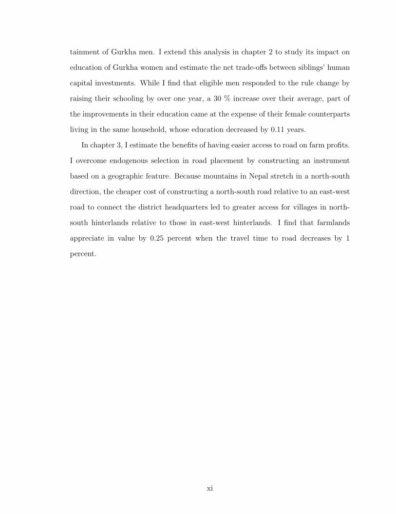
tainment of Gurkha men. I extend this analysis in chapter 2 to study its impact on

education of Gurkha women and estimate the net trade-o↵s between siblings’ human

capital investments. While I find that eligible men responded to the rule change by

raising their schooling by over one year, a 30 % increase over their average, part of

the improvements in their education came at the expense of their female counterparts

living in the same household, whose education decreased by 0.11 years.

In chapter 3, I estimate the benefits of having easier access to road on farm profits.

I overcome endogenous selection in road placement by constructing an instrument

based on a geographic feature. Because mountains in Nepal stretch in a north-south

direction, the cheaper cost of constructing a north-south road relative to an east-west

road to connect the district headquarters led to greater access for villages in north-

south hinterlands relative to those in east-west hinterlands. I find that farmlands

appreciate in value by 0.25 percent when the travel time to road decreases by 1

percent.

xi

CHAPTER I

Human Capital Investment Responses to Skilled

Migration Prospects: Evidence from a Natural

Experiment in Nepal

1.1 Introduction

“Brain drain” describes the emigration of skilled workers, mainly from developing

to developed countries. It hinders countries’ long-run economic growth by depleting

their scarce human capital. In 2000 more than 12 million individuals from developing

countries with tertiary education, 20 percent of their educated workforce, were living

in OECD countries.

A new literature in skilled emigration emphasizes the e↵ect of future emigration

opportunities on human capital accumulation. The reasoning behind these “brain

gain” models is that migration prospects raise the expected returns to education and

encourage individuals at home to increase their human capital investment. If enough

skilled individuals eventually decide not to emigrate, it can lead to a net increase

in human capital stock at home.1 While these new theoretical predictions challenge

1Individuals could change their emigration decision in the future for various reasons. The mostpopular explanation put forward by earlier brain gain papers is that quotas set by immigrationauthorities in destination countries are binding. Hence, even if lots of individuals actively seekto emigrate in the future, most of them are forced to live in their home country. Other reasons

1

the negative view of skilled emigration, empirical evidence is scarce because migration

prospects are endogenous. This paper overcomes the problem by identifying a natural

experiment that exogenously and di↵erentially raised emigration prospects for skilled

versus unskilled individuals at home.

The experiment involves a change in the British Gurkha Army recruitment reg-

ulations. The British Gurkha Army is the unit of the British Armed Forces that is

composed of Nepali men of Monglo-Tibeto origins. According to Banskota (1994),

since 1857 the Monglo-Tibeto tribes have created a tradition of enlisting in the British

Gurkha Army, and thereby they are collectively referred to as the Gurkha ethnic

group.2 Furthermore, the economic and anthropological data from Nepal indicate

that this British colonial tradition still plays an important financial and cultural role

in the Gurkha communities of Nepal.3 In 1993 the British government changed the

educational requirement for the British Gurkha applicants, from requiring no edu-

cation to requiring a minimum of 8th grade education. This change was instigated

by the modernization of the British Army following the developments in Eastern Eu-

rope in the early 1990s and the growing use of technology in warfare, as indicated

by discussions in the House of Commons.4 The reform focused on reducing service

manpower and increasing technological capabilities, which were complemented by

improving training and education of soldiers. Because this change was part of the

broader restructuring of the British Army, the timing and the rationale for this change

is exogenous to social, economic, or political characteristics of Nepal. Therefore, it

why individuals change their emigration decision, include unanticipated future changes in individ-uals’ socio-economic characteristics as well as changes in their preferences which a↵ect their futureemigration choices.

2All the remaining ethnicities in Nepal, excluding the Gurkha ethnic group, are referred to asthe “non-Gurkha” ethnic group for the remainder of this paper.

3For detailed documentation for the cultural significance and the financial contribution of theBritish Gurkha among Gurkha communities of Nepal, see Hitchcock (1966); Caplan (1995).

4For detailed documentation of the strategic defense reviews presented to the House of Com-mons regarding the restructuring of the British Army in early 1990s, together with the debate anddiscussions that followed, see the Eighth Defense Review. http://www.parliament.the-stationery-o�ce.co.uk/pa/cm199798/cmselect/cmdfence/138/13802.htm

2

provides a simple natural experiment where Gurkha men experienced an exogenous

increase in skilled emigration prospect relative to unskilled emigration to a foreign

labor market i.e. the British Army.

My empirical approach improves identification compared to the strategies used

in previous studies. The problem in estimating the impact of skilled emigration

prospects on education arises for two reasons: first, unobserved characteristics, such

as cultural norms and values, a↵ect both migration and schooling decisions; and

second, an increase in human capital raises migration incentives by reducing the

domestic wage for skilled workers. Beine et al. (2006) address this problem by in-

strumenting current migration prospects with the past emigrant stock. But the same

time-invariant characteristics that a↵ect migration prospects and necessitate the use

of an instrumental variable strategy are also likely to have a↵ected migration in the

past, thus undermining the validity of their historical instrument. While McKen-

zie and Rapoport (2006) argue that historical migration rates within Mexico are the

outcome of early 20th century railroad networks, it could still be problematic if past

migration led to a better assimilation of foreign ideas, such as value of education,

or if individuals with similar characteristics came to live together in regions with

better access to railroads. Therefore, the ideal experiment would require two groups

of individuals from developing countries that are identical except that skilled emi-

gration prospects exogenously increase for one of them.5 The change in education

requirement of the British Gurkha Army created such an experiment.

Using Nepal Census data from 2001, I identify individuals’ ethnicity to determine

whether they were a↵ected by this rule change. Since age-invariant ethnic characteris-

5To my knowledge, the only previous study to use a historical event for identification is Chand andClemens (2008). They use the unexpected coup in Fiji as a source of variation to study the e↵ect ofemigration prospects on education. However, in contrast to my experiment, emigration prospects forthe treatment group did not change exogenously but instead they argue that the decline in economicopportunity at home due to political instability created greater incentive for them to emigrate. Inresponse, they invested in education that increased their likelihood of successfully emigrating tocountries such as Australia.

3

tics could a↵ect education, I use their age at the time of the rule change as the second

criteria to determine their exposure. Given the recruits must be between the age of

171

2

and 21 years old, only men who were 21 or younger in 1993 could be a↵ected by

the rule change. I refer to these cohorts as the “eligible” cohort and older cohorts

as the “ineligible” cohort in this paper. The di↵erence-in-di↵erence strategy controls

for all age-varying characteristics and age-invariant ethnic characteristics that could

be correlated with education. As an alternative strategy, I use the synthetic control

method developed by Abadie and Gardeazabal (2003) by constructing a comparison

for the Gurkha ethnic group based on ineligible cohorts’ ethnic characteristics. The

results suggest that the change in the educational requirement induced Gurkha men

of cohorts aged 6 to 12 at the time of the rule change to raise their education by 1.11

years and cohorts aged 13 to 21 by 0.39 years. The estimates are consistent across

the two strategies, highlighting the robustness of my empirical findings. More impor-

tantly, the rule change did not increase migration rates of eligible Gurkha men and

increase in schooling also occurred for eligible Gurkha men who had not emigrated

by 2001, which means that the rule change increased the net human capital stock of

eligible Gurkha men.

My findings show that skilled emigration can lead to a net increase in human capi-

tal at home, by highlighting a positive impact of migration prospects on human capital

investment. The early literature in skilled emigration ignore this relationship and fo-

cus solely on the loss of human capital from emigration of skilled workers, thereby

concluding that skilled emigration is detrimental to home country’s human capital

accumulation.6 By assuming that productivity increases with greater concentration

of skilled workers, the endogenous growth models of Miyagiwa (1991) and Haque and

Kim (1995) also predict negative impacts on economic growth. However, Mountford

(1997) and Stark et al. (1997) show that endogenizing human capital accumulation

6Bhagwati and Hamada (1974) propose the brain drain tax to compensate for the loss incurredby developing countries due to skilled emigration.

4

on migration prospects, could raise net human capital stock of low income countries

and improve their economic growth if some skilled individuals eventually decide not

to emigrate. Since the recruitment was limited to 300 individuals annually, majority

of eligible Gurkha men did not join the British Gurkha Army. Therefore, my findings

are consistent with the theoretical predictions and overturn the pessimistic outcomes

of the earlier models.

While Foster and Rosenzweig (1996) and Kochar (2004) show that schooling

choices are a↵ected by educational returns at home, my paper extends their anal-

ysis beyond political boundaries into foreign labor markets. I develop a theoretical

model of human capital and emigration decisions, highlighting the three important

factors that drive my results. First, there is a significant increase in income through

emigration; second, there is an educational requirement to emigrate; and third, the

likelihood of successfully emigrating is low. These three factors, which propelled el-

igible Gurkha men to invest in education and led to a net increase in their human

capital following the rule change, are also the main drivers of brain gain in other

developing countries. Beine et al. (2006) argue that large income di↵erences between

developing and developed countries increase the perceived benefits of migration, and

induce emigration in developing countries. According to Docquier et al. (2007), popu-

lar destination countries such as Australia, Canada, the United Kingdom, and the EU

employ skill-biased immigration policy, thereby making skilled emigration the most

feasible way for individuals from developing countries to emigrate. They also find

that the skilled emigration rate in developing countries in 2000 was only 7%, despite

an increase of 70% over the previous decade. In line with my findings, Chand and

Clemens (2008) show that skill-selective points systems used by immigration author-

ities of Australia and New Zealand induced Fijians to invest in education, resulting

in a net increase in the human capital stock of Fiji. Therefore, the underlying mecha-

nisms of my unique natural experiment are consistent with economic forces a↵ecting

5

individuals’ education and migration choices in many developing countries.

The rest of the paper is structured as follows: Section 2 describes the natural

experiment. Section 3 presents a theoretical framework that forms the basis of brain

gain models. Section 4 explains the empirical strategy and the data used for causal

estimation. Section 5 presents the empirical results. Section 6 presents robustness

for the identification strategy and Section 7 concludes.

1.2 Background

Nepal is a landlocked country surrounded by India on three sides and China to

its north. Its geographical position historically made it a melting ground for people

and cultures from both north and south of its border (Shrestha, 2001b). The 1996

National Living Standard Survey categorizes the population of Nepal into 15 ethnic

groups. Out of them, the Gurkha ethnic group is comprised of 5 Monglo-Tibeto tribal

groups– the Rai, Limbu, Gurung, Magar, and Tamang, who settled in the eastern

and central hills of Nepal during the initial wave of migration from the north.

1.2.1 British Brigade of Gurkha

The British Brigade of Gurkha is the unit in the British Army that is composed

of Nepali soldiers. Following the Anglo-Gurkha war (1814-1816), the British East

India company and the Government of Nepal signed the treaty of Sugauli on March

4, 1816. The treaty transferred one-third of the territories previously held by Nepal

to the British and allowed them to set up three Gurkha regiments in the British

Indian Army.7 The early recruits of the British Gurkha Army included ethnic groups

such as the Rajput, Thakuri, Chetri, and Brahman, who migrated from the south

and were closely associated with the ethnicities of India. In 1857, Indian soldiers

serving in the British Indian Army led a mutiny against British rule in South Asia.

7For details of the Sugauli Treaty see Rathaur (2001).

6

Although the rebellion was eventually contained in 1858, the British became wary

of Indian nationals serving in their army. Rathaur (2001) and Caplan (1995) argue

that, as a result, the British stopped recruiting Nepali individuals belonging to the

ethnicities that originated from India into the British Gurkha Army. According to

Rathaur (2001) after 1857, the new Nepali recruits were mainly drawn from the Rai,

Limbu, Gurung, Magar, and Tamang ethnic groups who, unlike other ethnicities in

Nepal, had migrated from north and had no cultural or historical ties with India.8

This ethnicity bias in the recruitment of British Gurkha Army continues to exist to

the present day as the majority of the current British Gurkha soldiers are comprised

of these 5 Monglo-Tibeto tribes. Although the British government no longer uses

ethnicity as a criteria for selection, the de facto ethnicity bias could be due to the lack

of information on recruitment available for non-Gurkhas, or because non-Gurkhas are

marginalized in the recruitment process as the first stage of selection is conducted by

ex-Gurkha servicemen who are themselves from Gurkha ethnic group. Consequently,

this British colonial tradition has evolved into an important cultural identity and

lucrative economic opportunity for the individuals of the Gurkha ethnic group. The

present value of the lifetime income from serving in the British Gurkha Army for

25 years is estimated to be $ 1,334,091.81.9 This includes a starting salary of $

21,000 and a lifelong annual pension of about $ 15,000 after retirement. According to

Caplan (1995), remittances from Gurkha soldiers and pensions for ex-Gurkha soldiers

were the country’s largest earner of foreign currency until the recent development of

tourism and other sources of migration. Although every year there are only 300

successful applicants, the pay and pensions of the servicemen are the major source

8The preference for Gurkha ethnic men is evident from the letter by the British CommandingRecruitment O�cer to Colonel Berkely, the British Resident at Kathmandu, in the early 1900s inwhich he writes, “I first consider his caste. If he is of the right caste, though his physique is weak, Itake him” (Banskota, 1994).

9See Table 1.10 for estimation of the lifetime income for Gurkha soldiers. Other non-financialbenefits include the opportunity to permanently settle in the UK along with immediate familymembers.

7

of capital in most Monglo-Tibeto communities in the hills of Nepal, mainly because

their alternative employment is limited to farming.10 The financial benefits of the

British Gurkha Army in these communities is evident from quotes from the Gurkha

households documented by Caplan (1995) such as, “One of my boys has gone to the

Army, we have only that hope.”

Although the appeal of joining the British Gurkha Army is driven by economic

benefits, it also brings cultural prestige to Gurkha communities. Caplan (1995) points

out that Gurkha ex-servicemen as well as their wives are known in their villages by

their titles of the British Army and acquire considerable reputations to become the

new elite in their communities. Hitchcock (1966) reports that many Gurkha villages

are named after the title of their highest ranking British Gurkha o�cer, such as

“the Captain’s village.” These narratives highlight the social, political, and economic

stature wielded by the British Gurkha Army in Gurkha communities of Nepal.

1.2.2 Natural Experiment: A Change in Education Criteria

Education is an important aspect of the British Gurkha recruitment. Starting

from 1993, recruits must have completed at least 8 years of education.11 Prior to this,

however, no formal education was required to join the British Army and the selection

criteria was strictly limited to physical examinations. This change in the education

requirement was instigated by the larger restructuring of the British Army in the early

1990s. Following the end of the cold war, a series of defense reviews termed “Option

for Change” was conducted by the UK Ministry of Defense in order to evaluate the

role of its army in the post-cold war era. It focused on reducing defense expenditure

spurred by the economic benefits of the “peace dividend”12 and, consequently, led to

10The Defense Committee of the House of Commons in 1989 suggested that the annual salary ofBritish Gurkha soldier was 100 times the average income in the hills from where they come from.

11In 1997, the education requirement was further increased to a minimum of 10 years of education.12Peace dividend is a political slogan popularized by US president George H.W. Bush and UK

Prime Minister Margaret Thatcher after the end of the cold war. It describes the reduction indefense spending undertaken by many western nations, including as the US and the UK, and the

8

a reduction in service manpower of the British Army by 18 percent. Furthermore, this

reduction was accompanied by the emphasis on a flexible and modernized force. This

was achieved by incorporating new technologies in weapon systems, communications,

reconnaissance missions, and intelligence gathering, and by improving education and

training of soldiers. The Option for Change outlined the use of technology in future

warfare and the importance of education for soldiers who use it, and concluded that

“strong defense requires military capability of fighting in a high-technology warfare;

the aim is smaller forces, better equipped, and properly trained” (Eighth Defense

Report, 1997). In fact, the trend towards educated soldiers had already begun in the

US Army, as its recruits with a high school diploma increased by 30 percent in the

late 1980s.13 Hence, the increase in educational requirement for the British Gurkha

was induced by the modernization of the British Army in response to the increasing

role of technology and the political changes in Eastern Europe and, therefore, it was

exogenous to the socio-political events in Nepal.

1.3 Theoretical Model

Becker’s model of human capital views education as an investment, where indi-

viduals compare their costs to future benefits. The future benefits from investing

in education is an increase in lifetime income earned domestically when there is no

opportunity to emigrate. Given positive emigration prospects, however, the future

benefits should additionally include expected increase in income earned abroad. Fur-

thermore, the latter could be larger if either the wage rate per human capital is

higher abroad, or income abroad at all levels of education is greater and education

is required to emigrate, or both. The following theoretical model, based on Docquier

subsequent redirection of those resources into social programs and a decrease in tax rates.13According to the Tenth Quadrennial Review of US Military Compensation, the recruits who

scored better than the median in the Armed Forces Qualification Test (AFQT) increased by 10% inearly 1990s.

9

et al. (2007), highlights these positive e↵ects of higher skilled emigration prospects

on expected returns to schooling and, consequently, on educational investment and

net human capital stock.

Consider a small developing economy, where labor is an important factor of pro-

duction and is measured in e�ciency units. All individuals at birth are endowed

with a unit of e�ciency. They live for two periods, youth and adulthood. There is

an education program which if opted into during youth, increases the individual’s

e�ciency in adulthood to h > 1. Furthermore, the heterogeneity among individu-

als is highlighted by the di↵erences in their cost of the education program, denoted

by c, which has a cumulative distribution F (c) and density function f(c) defined on

R+. Suppose the domestic economy is perfectly competitive so that workers are paid

their marginal product, denoted by w. In youth, uneducated workers earn w and

educated workers earn w � c. In adulthood, individuals can choose to work abroad,

where the wage rate per e�ciency unit is w > w and the income premium is I >

0. In adulthood, uneducated workers can either earn w + I if they migrate or w if

they don’t. Likewise, educated workers can earn wh + I if they migrate and wh if

they don’t migrate. Individuals incur a fixed cost in adulthood if they attempt to

emigrate, denoted by M . Let the probability of migration, denoted by p, be the same

for both educated and uneducated workers. Suppose (w+ I�w) � M

p

, which implies

that all individuals would choose to emigrate.14

If individuals are risk neutral so that they choose their education to maximize

14The condition for all educated workers to choose to migrate is wh + I � wh � Mp and for

uneducated worker, it is w+ I �w � Mp . These conditions imply that an increase in income due to

migration should be greater or equal to the ratio of the cost and probability of migration. Accordingto the UK Defense Committee, the annual salary of a British Gurkha soldier in 1989 was 100 timesthe average income in Nepal. Furthermore, the financial cost of applying for the British Gurkha isminimal as there is no application fee and the recruiters visit most Gurkha villages every year duringthe first stage of selection process. Moreover, the empirical estimate is interpreted as the averagetreatment e↵ect on all age eligible Gurkha men, regardless of their future intention of applying tothe British Gurkha.

10

lifetime income, then the condition for investing in education becomes:

w � c + (1� p) wh + p (wh+ I) �M > w + (1� p) w + p (w + I) �M

and individuals will invest in education if and only if:

c < cp

⌘ w(h� 1) + p (w � w) (h� 1) (1.1)

The critical threshold cp

is increasing in the probability of migration p, which

implies that migration prospects raise the expected return to education and induce

more individuals in developing countries to invest in education. Furthermore, this

incentive e↵ect is larger, greater the international wage di↵erence (w � w). The

share of adult domestic workers who opted for education in their youth is given by

Hp

= F (Cp

).

Now, suppose the migration probability changes di↵erentially across educated

and uneducated workers.15 In line with the change in the British Gurkha education

requirement, the migration probability is assumed to be still p for educated workers

but p for unskilled workers, where p equals zero. The probability p is assumed to be

exogenously determined by the service requirement of the British Army independent

of schooling decisions of individuals at home.16 Uneducated workers remain at home

and therefore earn domestic wage w in both periods. In contrast, educated workers

earn w � c in their youth and once adult they can earn either wh + I � M if they

15Prior to the rule change in 1993, both educated and uneducated workers had equal probabilityof joining the British Gurkha Army. Furthermore, since the selection criteria were solely basedon physical attributes, education did not increase one’s chance of getting selected. Following therule change in 1993, however, only individuals with required education level could apply; whereas,individuals with less than 8 years of education could no longer apply to the British Gurkha.

16The probability p can be a decreasing function of cs(p) in (2), defining an implicit solution forp. The response to the rule change is partly determined by individual’s expectation of how otherswould response to the rule change, which in turn a↵ect their perceived p. The perceived and actualprobability after the rule change will either stay the same or increase.

11

migrate or wh�M if they don’t.17 The new condition for investing in education is:

w � c + (1� p) wh + p (wh+ I) �M > w + w

and individuals will opt for education if and only if:

c < cs

⌘ w(h� 1) + p (w � w) h + p I �M (1.2)

The new critical threshold cs

is increasing in skilled emigration probability p, the

di↵erence in wage (w � w), and the foreign income premium I. If I � M

p

, it implies

that cs

> cp

because individuals who could emigrate without education previously, are

now prompted to invest in education in order to earn income premium abroad. To sum

up, emigration prospects raise expected returns to education because of higher wage

rate abroad, and skilled emigration relative to unskilled emigration prospects further

increase expected returns to education because only skilled workers can emigrate and

earn the higher income premium.

After pF (Cs

) fraction of workers migrate abroad in their adulthood, the share of

educated workers who are unable to emigrate relative to all domestic adult workers

is:

Hs

=(1� p) F (C

s

)

1 � pF (Cs

)

and Hs

> Hp

if and only if:

p < ep ⌘ F (Cs

) � F (Cp

)

F (Cs

) (1� F (Cp

))(1.3)

ep < 1 denotes the critical threshold probability of emigration for which the incen-

tive e↵ect of brain gain exceeds the negative e↵ect of brain drain. Given an extremely

17Similar to the previous case, assume wh + I � wh � Mp , so that all educated workers would

choose to migrate.

12

low likelihood of getting selected into the British Gurkha Army, the probability of

skilled emigration through the Gurkha recruitment is likely to be below ep, suggesting

that the rule change would create a net gain in human capital.

1.4 Identification Strategy

The change in the educational requirement in 1993 compelled new recruits to com-

plete at least 8 years of education in order to be eligible for the British Gurkha and,

thereby, increased their skilled emigration prospect relative to unskilled emigration.

The theoretical analysis above suggests that this rule change would increase expected

returns to education and induce individuals to invest in human capital. Furthermore,

because the rule change was exogenous to the socio-economic characteristics of Nepal,

the empirical strategy of comparing the education outcome of individuals who were

a↵ected to those who were not a↵ected by the rule change gives an unbiased estimate

of its e↵ect on domestic schooling.

The individuals’ exposure is jointly determined by their sex, ethnicity, and age.

First, the British Gurkha, in contrast to the other regiments of the British Army,

is exclusively made up of men; therefore, women were not a↵ected. Second, because

recruits must be between 171

2

and 21 years old, men who were 22 or older in 1993 were

not a↵ected by the rule change.18 Third, considering most British Gurkha soldiers

since 1857 have been Gurkha ethnic men, non-Gurkha men were also not a↵ected.

Hence, the e↵ect of rule change on age eligible Gurkha ethnic men is identified via

di↵erence-in-di↵erence estimation, comparing male education between eligible and

ineligible cohorts, within Gurkha and non-Gurkha ethnic groups. The di↵erence in

education between the two cohorts in the Gurkha ethnic group could be correlated

with the age-varying unobserved variables. Therefore, subtracting from this the co-

18As mentioned earlier, cohorts 22 and older are referred to as the “ineligible” cohort and cohorts21 and younger are referred to as the “eligible” cohort.

13

hort di↵erence in education for non-Gurkha ethnic men would net out all age-varying

characteristics as well as age-invariant ethnic characteristics that could directly a↵ect

education. The identification assumption is that in absence of this rule change in

1993, the evolution of education outcomes of men between the two cohorts would not

have systematically di↵ered across Gurkha and non-Gurkha ethnic groups. Further-

more, the di↵erence-in-di↵erence estimate of female education between the two ethnic

groups and cohorts serves as a false experiment to test this identification assumption.

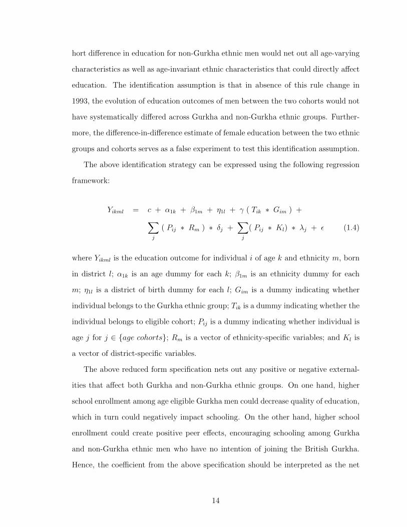
The above identification strategy can be expressed using the following regression

framework:

Yikml

= c + ↵1k

+ �1m

+ ⌘1l

+ � ( Tik

⇤ Gim

) +X

j

( Pij

⇤ Rm

) ⇤ �j

+X

j

( Pij

⇤ Kl

) ⇤ �j

+ ✏ (1.4)

where Yikml

is the education outcome for individual i of age k and ethnicity m, born

in district l; ↵1k

is an age dummy for each k; �1m

is an ethnicity dummy for each

m; ⌘1l

is a district of birth dummy for each l; Gim

is a dummy indicating whether

individual belongs to the Gurkha ethnic group; Tik

is a dummy indicating whether the

individual belongs to eligible cohort; Pij

is a dummy indicating whether individual is

age j for j 2 {age cohorts}; Rm

is a vector of ethnicity-specific variables; and Kl

is

a vector of district-specific variables.

The above reduced form specification nets out any positive or negative external-

ities that a↵ect both Gurkha and non-Gurkha ethnic groups. On one hand, higher

school enrollment among age eligible Gurkha men could decrease quality of education,

which in turn could negatively impact schooling. On the other hand, higher school

enrollment could create positive peer e↵ects, encouraging schooling among Gurkha

and non-Gurkha ethnic men who have no intention of joining the British Gurkha.

Hence, the coe�cient from the above specification should be interpreted as the net

14

e↵ect of the rule change on age eligible Gurkha ethnic men.19 Furthermore, since the

information regarding individual’s decision to apply for the British Gurkha are not

available, the coe�cient is also the average treatment e↵ect from the rule change on

all age eligible Gurkha men, regardless of their future intention of applying for the

British Gurkha.

The identification strategy can also be generalized to examine the impact of the

rule change for each birth-year cohort in the following regression framework:

Yiklm

= c + ↵1k

+ �1m

+ ⌘1l

+X

x

( Pix

⇤ Gim

) ⇤ �x

+

X

j

( Pij

⇤ Rm

) ⇤ �j

+X

j

( Pij

⇤ Kl

) ⇤ �j

+ ✏ (1.5)

Each �x

can be interpreted as the e↵ect of the rule change on Gurkha men of age

x. Since men who were 22 and older were not a↵ected, the coe�cients �x

should be 0

for x � 22. Additionally, the coe�cients �x

should increase as x decreases for x < 22.

Younger age eligible Gurkha men were more likely to be enrolled in school at the time

of the rule change and had more time to complete 8th grade education, putting them

in a better position to respond to the rule change compared to older age eligible men.

The data required for the above identification strategy are obtained from 2001

Nepal Census for individuals aged 6 to 44 in 1993. It also includes information for

individuals who were living abroad in 2001, abating the concern for potential bias

due to selective attrition.20 The census data are supplemented with Nepal Living

Standard Survey (NLSS) from 1996, which is a household sample survey with greater

19Given Figure 1.1 suggests that Gurkha ethnic group is concentrated in specific regions of Nepal,the externalities generated by the response to the rule change is also more likely to be experiencedby Gurkhas rather than non-Gurkhas. In this case, the estimated e↵ect of the rule change shouldbe interpreted as an overall e↵ect on eligible Gurkha men, with a combination of the net e↵ect ofthe rule change and net externality among Gurkhas generated by the rule change.

20If the entire household moved abroad between 1993 and 2001, then the information on thoseindividuals are not available. However, the propensity for the entire household to move abroad isextremely low in Nepal.

15

detail. Table 1.1 presents summary statistics for the 1,389,705 individuals from the

2001 Census and the 3,373 households from the 1996 NLSS. The averages for some

socio-economic characteristics are provided for the entire sample as well as separately

for the Gurkha and non-Gurkha ethnic groups. The Gurkha ethnic group comprises

of 16 percent of the samples in both surveys. Panel A shows that the average level

of education for the Gurkha ethnic group is 3.28, which is slightly lower than the

non-Gurkha average of 4.24. Similarly, 18.2% of Gurkha individuals were born in

urban districts compared to 34.1% of non-Gurkhas. Panel B suggests that around the

time of the rule change, non-Gurkha households had better access to school facilities

than Gurkha households and 46.9% of non-Gurkha households were living in poverty

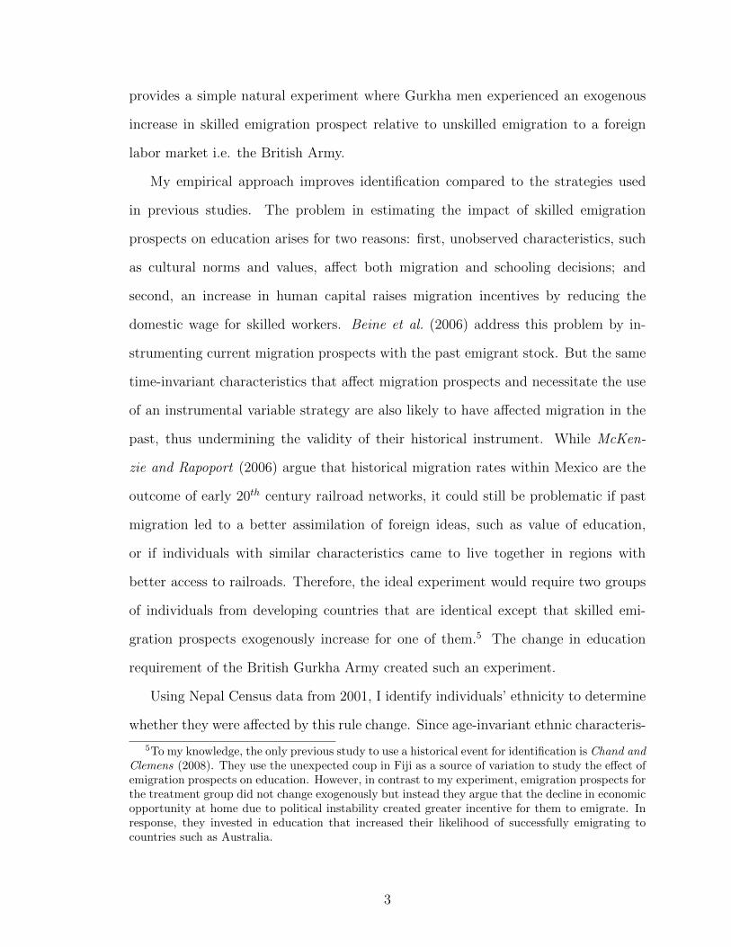
compared to 48.5% of Gurkha households. Figure 1.1 shows the map of Nepal with

the distribution of Gurkha ethnic group across 75 regional districts. It suggests that

most Gurkha households live in the northern central region and north east corner of

Nepal and predictably, the three British Gurkha recruitment centers are also located

within these regions.

1.5 Results

The identification strategy can be illustrated with a simple di↵erence-in-di↵erence

table between the eligible and ineligible cohorts in the Gurkha and non-Gurkha ethnic

groups. Table 1.2 compares educational attainment of Gurkha and non-Gurkha men

who were not a↵ected by the rule change (age 22 - 28) to those who were a↵ected,

either cohort aged 6 to 12 or cohort aged 13 to 21. I use eligible cohort aged 6 to 12

as the preferred cohort of analysis because this younger eligible cohort is most likely

to be enrolled in primary school in 1993 and also have enough time to change their

education in line with the new rule by the time they apply to the British Gurkha.

On the contrary, the ability of older eligible men aged 13 to 21 to respond to the rule

change is determined by the years of education that they have had completed in 1993.

16

For example, a Gurkha men of age 20 would only be able to successfully respond to

the rule change, if he had at least 7 years of education in 1993. Given the data on

their education in 1993 are not available, the older eligible cohort includes Gurkha

men some of whom were a↵ected by the rule change and others who were not.

In both ethnic groups, average education increased over time; but it increased

more in the Gurkha ethnic group. The simple di↵erence-in-di↵erence estimation

shows that Gurkha men of younger eligible cohort (aged 6-12) completed an average

of 1.2 more years of education. This is significantly di↵erence from zero at the 1%

level. Panel B shows that Gurkha men of older eligible cohort (aged 13-21) also

raised their education by 0.28 years, which is less compared to younger eligible cohort

but also expected due to the reasons discussed earlier. The two estimates are large

in magnitude especially for younger eligible cohort with an increase in education of

32% over the ineligible cohort. The positive impact of the rule change indicates that

the British Gurkha constitutes an attractive foreign labor market opportunity for

Gurkha men. Furthermore, it highlights the role of skilled emigration prospects on

increasing returns to education among individuals who might otherwise have limited

opportunity to benefit from education in the domestic labor market. This is especially

true for Gurkha recruitment as Caplan (1995) notes that most of the potential recruits

come from rural villages of Nepal and if not for the British Gurkha Army their best

alternative source of income is farming.

Tables 1.3 present the di↵erence-in-di↵erence analysis by estimating coe�cient

� in equation (1.4). The specification in column 1 controls for age dummies and

ethnicity dummies and the specification in column 2 additionally controls for district

of birth dummies. Figure 1.1 shows that Gurkha ethnic groups are concentrated in

the northern central region and north east corner of Nepal. If time-varying regional

characteristics are correlated with education, it could bias the above estimates. I

control for di↵erential evolution of geographic regions in columns 3, 4, and 5 by

17

including interactions of age dummies and district of birth dummies, for all ages

and districts. The specification in columns 4 and 5 also include interactions of age

dummies and district-level characteristics– total number of primary and secondary

teachers in 1994. Moreover, the specification in column 5 controls for additional

time-varying ethnic characteristic by including the interaction of age dummies and

ethnicity-level variable measuring the travel time to school, obtained from 1996 NLSS.

The errors in all specifications are clustered at the ethnicity level.

The estimates in Table 1.3, column 1 suggest that an increase in educational

requirement for the British Gurkha raised the education among younger eligible co-

hort by 1.19 years and older eligible cohort by 0.42 years, and both estimates are

statistically significant at the 1% level. More importantly, controlling for various

time-varying regional and ethnic characteristics do not change the magnitude and

the statistical significance of the estimates for both eligible cohorts, which makes it

unlikely that the results are driven by time-varying characteristics that are correlated

with education. The estimates in column 5, which includes all the controls mentioned

earlier, suggest that Gurkha men from younger eligible cohort raised their education

by 1.11 years and older eligible cohort by 0.39 years.

The above results rely on the assumption that in absence of the rule change,

the di↵erence of educational outcomes between the eligible and ineligible cohorts

would not have systematically di↵ered across Gurkha and non-Gurkha ethnic groups.

Table 1.4 presents a series of control experiments that compare educational attain-

ment between cohorts and ethnic groups that were not a↵ected by the rule change

and therefore, in contrast to the results in Table 1.3, should produce di↵erence-in-

di↵erence estimates of zero. Panel A compares education of ineligible cohort aged 22

to 28 with another ineligible cohort aged 29 to 35 across Gurkha and non-Gurkha

men. The estimate of coe�cient � in column 5 is 0.01 and not statistically di↵erent

from zero at the conventional levels. The control experiment in panel B considers

18

cohort aged 22 to 28 and cohort aged 38 to 44, so that the age di↵erence between the

two ineligible cohorts is consistent with the experiment in panel A of Table 1.2, in

which the age di↵erence between the younger eligible cohort and ineligible cohort is 9

years. The estimates are also not statistically di↵erent from zero in all specifications.

While Gurkha women might not be an appropriate control group due to potential

intrahousehold spillovers from an increase in education among Gurkha men, never-

theless, panel C compares education outcome for females aged 6 to 12 with 22 to 28,

in Gurkha and non-Gurkha ethnic groups. Based on table 1.4, column 5 the estimate

of the e↵ect of the rule change on Gurkha women of younger eligible cohort is -0.09

and not statistically di↵erent from zero. Given that all the estimates of coe�cient �

are not statistically di↵erent from zero, the results from table 1.4 support the validity

of the identification assumption and suggest that the increase in education for age

eligible Gurkha men in Table 1.3 is likely caused by the change in the educational

requirement for the British Gurkha recruitment.

Table 1.5 shows the e↵ect of the rule change for each eligible birth-year cohort by

estimating �x

s in equation (1.5) for 6 x 21. The comparison group consists of

ineligible cohort aged 22 to 28. In all specifications, the estimated e↵ect is statistically

significant at the 5% levels for Gurkha men 15 years or younger. The results in column

5 suggest that the rule change raised education for Gurkha men aged 15 by 0.69 years,

aged 12 by 0.95 years, and aged 6 by 1.38 years. Furthermore, in line with the natural

experiment, the e↵ect of the rule change increases with younger age due to the reasons

discussed in the earlier section. If the results are driven by the response to the rule

change, the estimated e↵ects would decrease with age for Gurkha men of eligible

cohort and be zero for all ineligible birth-year cohorts. I test this hypothesis by

estimating �x

s in equation (1.5) for 6 x 35. The control group comprises of men

aged 36 and 37. The estimates of �x

s are plotted in Figure 1.2. �x

s fluctuate around

zero and statistically insignificant for all x � 22 and increase as age decreases for

19

x 21, providing further support for the internal validity of the natural experiment.

The rule change induced eligible Gurkha men who had no formal education at the

time of the rule change, to enroll in school for the first time. Table 1.6 presents the

e↵ect at the extensive margin, by estimating the coe�cient � in equation (1.4) for

younger eligible cohort, where the dependent variable is a dummy indicating years

of education completed greater than zero. The results in column 5 suggest that the

proportion of young eligible Gurkha men with at least 1 year of education increased

by 10 percentage points. Given 51% of age ineligible Gurkha men have no formal

education, the rule change induced 19.5 percent of young eligible Gurkha men who

would not have received any formal education in the absence of the rule change, to

enroll in school. In comparison, Schultz (2004b) estimates that the Mexican Progresa

Program induced 10 percent of individuals who had no prior education to enroll in

school by reducing educational cost by as much as 75%.21

Individuals who were induced to enroll in school by the rule change and who

had already enrolled prior to the rule change, were further promoted to raise their

education because the new rule required 8 years of education. I estimate the impact at

di↵erent education levels by estimating the di↵erence in di↵erences in the cumulative

distribution function of education between young eligible and ineligible cohorts across

Gurkha and non-Gurkha men who have at least one year of education. Figure 1.3

depicts the estimates of �ss from equation (1.4), with a dummy dependent variable

indicating the level of education completed equal to or greater than s, for each s

= 2 to 15.22 Among Gurkha men of young eligible cohort with at least one year of

education, the share of those with 5 or more years (primary education) increased by 3

percentage points, 8 or more years (the requirement cuto↵) increased by 6 percentage

21These two results might not be directly comparable as PROGRESA started from higher enroll-ment base and targeted poorest students. Because of these reasons, increasing schooling might havebeen harder to achieve in the case of PROGRESA.

22The error terms in these 14 seemingly unrelated regression equations (SURE) are correlated.In Figure 1.3, the 95 percent confidence intervals for each �ss are adjusted for cross-equation errorcorrelation.

20

points, and 13 or more years (tertiary education) increased by 9 percentage points.

The large impact at upper end of the education distribution is particularly sig-

nificant, given Jensen (2010) points out that in developing countries a combination

of costs, low family income, and credit constraints provides a relatively greater hin-

drance to secondary schooling compared to primary education as it requires a longer

term and more costly investment. For example, while 67% of Nepali boys in 1996

were enrolled in primary school, the net enrollment rate in lower secondary level (6-8

years) was merely 23% (1996 NLSS). Additionally, the positive impact on education

above 8 years could be due to the further increase in the British Gurkha educational

requirement from 8 to 10 years in 1997, or because higher education increased the

likelihood of success with the introduction of English and mathematics exams in the

selection process, or because eligible Gurkha men who completed 8 years of education

to comply with the new rule continued into higher education. Angrist and Imbens

(1995) find similar positive spillover e↵ects in the United States, where the compul-

sory attendance laws induced a fraction of the sample to complete some college as a

consequence of constraining them to complete high school.

In developing countries, socio-economic factors such as access to schools, costs,

credit constraints, and family income, limit individuals from attending school even

when they want to. I examine the e↵ect of these factors on individuals’ response to

the rule change, by separately estimating equation (1.4) across di↵erent population

characteristics. The results in columns 2 and 3 of Table 1.7 indicate that the e↵ect of

the rule change did not vary across districts with and without easy access to schooling.

However, the di↵erence in average travel time to school between the bottom and top

quantile districts is only 0.3 hours, which reflects the emphasis put by the government

on improving access to school in remote areas of Nepal. The results in columns 4 and

5 indicate that the impact of the rule change was smaller for individuals living in

households that are involved in agricultural production. According to Nepal Living

21

Standard Survey from 2004, more than 10% of school-age children who were not

enrolled in school indicated labor constraint in household work as the main cause

of their absenteeism. Furthermore, more than 20% of the school absenteeism was

caused by high financial cost of education. In oder to examine the role of poverty and

credit constraints on schooling, columns 6 and 7 separately estimate the e↵ect of the

rule change across household income, using ownership of television set as a proxy for

family wealth. In households that own a television set, Gurkha men of young eligible

cohort raised their education by 1.28 years; whereas, their counterparts living in the

household without a television set only raised their education by 0.76 years. The

F-test suggests that estimates are statistically di↵erent at the 10% level. While these

results should be interpreted with caution due to omitted variable bias, the stratified

results, nevertheless, could be potentially informative given they document the role

of poverty and credit constraints in limiting schooling in developing countries.

The majority of eligible Gurkha men would not join the British Gurkha Army

because only 300 individuals are recruited every year. However, higher education

could increase emigration rates of eligible Gurkha men through other channels besides

the British Gurkha recruitment. I estimate coe�cient � in equation (1.4), with a

dummy dependent variable indicating whether the individual was living abroad in

2001. Given everyone in the older eligible cohort would have had the chance to apply

for the British Gurkha Army or pursue other emigration opportunities by 2001, I

focus on this cohort to examine whether the rule change led to greater emigration

among eligible Gurkha men. The estimates in Table 1.8, panel B suggest that there

was no increase in migration rates among older eligible Gurkha men. The coe�cients

in all the specifications are zero and not statistically significant even at the 10% level.

On the other hand, Table 1.9 estimates the e↵ect of the rule change on education

of eligible Gurkha men who had not emigrated by 2001. I estimate coe�cient � in

equation (1.4) by only including individuals who were living in Nepal in 2001. The

22

results in column 5 suggest that the rule change raised education of young eligible

Gurkha men who had not emigrated by 1.14 years and older eligible Gurkha men of

similar nature by 0.40 years. Both the estimates are statistically significant at the 1%

level. Therefore, the results in Tables 1.8 and 1.9 together imply that the increase

in educational requirement for the British Gurkha Army led to a net increase in the

human capital stock of eligible Gurkha men.

1.6 Robustness

In the above empirical estimation, the non-Gurkha ethnic group may not be a

valid comparison for the Gurkha ethnic group because ineligible Gurkha cohorts have

significantly lower level of education than their non-Gurkha counterparts. To re-

fute the possibility that the results could be driven by age-varying unobserved ethnic

characteristics, I use a data-driven procedure developed by Abadie and Gardeazabal

(2003) to construct a di↵erent comparison group. The new counterfactual– the syn-

thetic Gurkha ethnic group– is the convex combination of all non-Gurkha ethnicities

that most closely resemble the Gurkha ethnic group based on the education of age

ineligible men. For each non-Gurkha ethnicity, the average years of education is cal-

culated for each birth cohort and then ethnicity-weights are assigned to minimize the

di↵erence between education of Gurkha and synthetic Gurkha ethnic groups across

ineligible cohorts aged 22 to 44.23 Table 1.11 displays the weights of each non-Gurkha

ethnicity in the synthetic Gurkha ethnic group.

Figure 1.4 depicts the years of education completed for Gurkha and synthetic

Gurkha ethnic groups across birth cohorts aged 6 to 44. Education of the synthetic

Gurkha ethnic group closely matches that of the Gurkha ethnic group for ineligible

23The ethnicity-weights are calculated from the minimization problem: Choose W to minimize(XG �XNW )(XG �XNW ), where W = {(w1, .....wJ)0 subject to w1 + .....+wJ = 1, wJ � 0}. XG

is a (k X 1) vector of average years of education at each age ineligible birth cohorts for the Gurkhaethnic group, where 21 k 44. XN is a (k X J) matrix with average years of education for kineligible birth cohorts and J non-Gurkha ethnicities.

23

cohorts aged 22 to 44, suggesting that the eligible cohort of synthetic Gurkha ethnic

group provide a close approximation to the eligible cohort of Gurkha ethnic group

in the absence of the rule change. The di↵erence in education between Gurkha and

synthetic Gurkha ethnic groups for cohorts aged 6 to 21 could be interpreted as

the e↵ect of the increase in the British Gurkha education requirement. Figure 1.5

shows that education between Gurkha and synthetic Gurkha ethnic groups diverges

considerably for eligible cohorts and the gap, depicted in Figure 1.5, becomes larger for

younger cohorts, which is consistent with the results from the di↵erence-in-di↵erence

estimation.

The results could have also been obtained entirely by chance. Following Bertrand

et al. (2004), I iteratively apply the synthetic control method to all the non-Gurkha

ethnicities to examine whether assigning treatment at random produces results of

similar magnitude. In each case, the synthetic control is composed of the weighted

combination of the remaining non-Gurkha ethnicities. Figure 1.6 displays the results

of the placebo iterations for 10 non-Gurkha ethnicities. The faded lines show the

gap in education between each non-Gurkha ethnicity and its corresponding synthetic

version. The gap for Gurkha ethnic group, depicted by the dark line, is largest com-

pared to any non-Gurkha ethnicities. More importantly, the education gap between

Gurkha and synthetic Gurkha for eligible cohort is four times larger than the similar

gap for ineligible cohort. Figure 1.7 shows that this is largest among all ethnicities.

Given there are 11 di↵erent ethnicities, including Gurkha ethnic group, and thereby

11 di↵erent results, the probability of obtaining the largest e↵ect for Gurkha ethnic

group entirely by chance is 1/11 = 0.09. Therefore, it is unlikely that the estimated

e↵ect of the rule change on age eligible Gurkha men could have occurred entirely by

chance.

24

1.7 Conclusion

The change in the educational requirement for the British Gurkha Army in 1993

led to an exogenous and di↵erential increase in skilled versus unskilled emigration

prospects for Gurkha men of eligible cohort living in Nepal. Using a set of di↵erence-

in-di↵erence and synthetic control strategies, I find that they responded to the rule

change by raising their human capital investment. I also find that the rule change

increased education for eligible Gurkha men who had not joined the British Gurkha or

emigrated elsewhere by 2001. These two findings validate the theoretical predictions

of the brain gain models: first, individuals’ human capital investments are endogenous

to their migration prospects; and second, when enough skilled individuals eventually

decide not to emigrate, it leads to a net increase in human capital stock at home.

The underlying mechanism of my unique natural experiment is not di↵erent from

economic factors influencing individuals’ emigration and human capital decisions in

many developing countries. Despite an extremely low chance of getting selected into

the British Gurkha Army, Gurkha men were induced to invest in education following

the rule change because of significant increase in income if they succeeded in joining

the British Army. Docquier et al. (2007) point out that these two factors, widening

international wage gaps and introduction of skilled-biased immigration policies, are

the main reasons for a rapid growth of skilled emigration and for inducing human

capital investment among potential emigrants in developing countries. Nevertheless,

they find that in 2000 the skilled emigration rate in developing countries was only

7%.

While the knowledge of the British Gurkha rule change was widespread, similar

information about other foreign labor markets may not be as readily available. Jensen

(2010) show that the lack of information regarding returns to education could lead

to underinvestment in human capital. Therefore, it might require an e�cient flow

of information possibly through an active government intervention for individuals at

25

home to know their educational returns abroad, and consequently, to increase their

human capital investment.

An important implication of my findings is that low-income countries do not

have to wait for improvements in their local productivity to stimulate human capital

investment because high wages in developed countries can motivate individuals in

developing countries to invest in education. While there is little doubt that low levels

of schooling deter economic growth, Schultz (1975) show that returns to schooling are

low in a stagnant economy, hinting at the possibility of a poverty trap. Oyelere (2009)

argue that poor institutions and political instability, characteristics that are common

across many developing countries, lead to low returns to education. Developing coun-

tries spend large sums of money on increasing human capital investment in order to

overcome low returns and push themselves out of the poverty trap, if it exists. For

example, Mexico’s Progresa Program which provides cash incentive to increase school

attendance, costs almost 0.2 percent of its GDP. Since skilled emigration prospects

raise educational returns in developing countries, it could either replace expensive

policy interventions like Progresa or complement these programs, making them more

attractive to their potential recipients.

Interesting future research includes investigating the welfare impact on eligible

Gurkha men who who could not join the British Gurkha Army. Increase in their edu-

cation could raise their domestic earnings, improve their children’s health outcomes,

and promote long-term economic growth in their regions. Similarly, the rule change

also created numerous positive and negative externalities on other populations that

were not directly a↵ected by it. First, an increase in education by Gurkha men could

directly a↵ect their peers’ education decisions. On one hand, it decreases the quality

of education by crowding out classrooms; whereas, on the other hand, greater class

participation could lead to a positive learning experience for other classmates. This

provides a useful experiment to investigate peer e↵ects, which is an integral part of

26

education research. Second, raising Gurkha men’s education could also a↵ect the

education of their siblings, mainly female siblings who were not a↵ected by the rule

change. Given key socio-economic decisions including children’s education are taken

at household-level, investigation into the specific mechanisms governing this intra-

household tradeo↵s is important. It would allow for better evaluation of existing

household interventions and development of more e↵ective policies in the future.

27

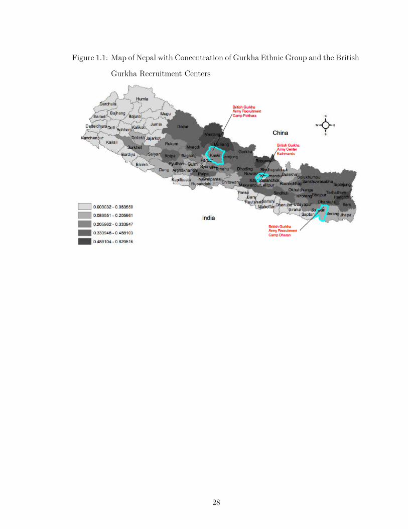
Figure 1.1: Map of Nepal with Concentration of Gurkha Ethnic Group and the British

Gurkha Recruitment Centers

28

Figure 1.2: E↵ect of the Rule Change on Human Capital Investment of Gurkha Men

at Each Birth Cohort (Identification Test)

-10

12

6810121416182022242628303234Age in 1993

Notes: The figure above plots �x

s for 6 x 35 from equation (1.5). Since each �x

estimates the e↵ect of the rule change on Gurkha men of age x in 1993, �x

should bezero for x � 21 and increase as x decreases for x < 21.

29

Figure 1.3: Di↵erence in Di↵erences in CDF (Estimated from Linear Probability

Model) with 95-Percent Confidence Interval

0.0

5.1

.15

.2.2

5

2 3 4 5 6 7 8 9 10 11 12 13 14Years of Education

Notes: The figure plots �s estimated from equation (1.4) with a dummy dependentvariable indicating the years of education completed greater than or equal to s, foreach s = 2 to 14. The error terms in these 14 seemingly unrelated regression equations(SURE) are correlated. The 95 percent confidence intervals for each �ss are adjustedfor cross-equation error correlation. The sample includes men from younger eligiblecohorts aged 6 to 12 or ineligible cohort aged 22 to 28, with at least 1 year of educationcompleted. Each �s indicate the impact of the rule change at the education level samong Gurkha men of younger eligible cohort with at least 1 year of schooling.

30

Figure 1.4: Comparison between Gurkha and Synthetic Gurkha

02

46

Year

s of

Edu

catio

n

68101214161820222426283032343638404244Age in 1993

Gurkha Synthetic Gurkha

Notes: The graph above plots the average years of education completed as of 2001at each birth cohort for Gurkha and synthetic Gurkha ethnic groups. The syn-thetic Gurkha is a weighted sum of all the non-Gurkha ethnicities. The weightsare calculated to minimize the squared di↵erence in average education of Gurkhaand synthetic Gurkha ethnic groups across birth cohorts aged 22 to 44. Basedon the mathematical algorithm provided by Abadie and Gardeazabal (2003), I chooseW to minimize (X

G

� XN

W )(XG

� XN

W ), where W = {(w1

, .....wJ

)0 subject tow

1

+ ..... + wJ

= 1, wJ

� 0}. XG

is a (k X 1) vector of average years of educationat each age ineligible birth cohorts for the Gurkha ethnic group, where 21 k 44.X

N

is a (k X J) matrix with average years of education for k ineligible birth cohortsand J non-Gurkha ethnicities.

31

Figure 1.5: Comparison between Gurkha and Synthetic Gurkha (Gap)

-.50

.51

Gap

in Y

ears

of E

duca

tion

68101214161820222426283032343638404244Age in 1993

Notes: The figure plots the di↵erence between average education of Gurkha andsynthetic Gurkha ethnic groups for each birth cohorts aged 6 to 44, i.e. the di↵erencebetween the education trends of the two groups from Figure 1.4.

32

Figure 1.6: Significance Test: Gap for Gurkha and 10 Placebo Gaps for Non-Gurkha

Ethnicities

-2-1

01

2Ga

p in

Yea

rs o

f Edu

catio

n

68101214161820222426283032343638404244Age in 1993

Notes:The figure plots the gaps same as Figure 1.5 for Gurkha ethnicity in the darkline and similar gaps for 10 non-Gurkha ethnicities in faded lines. For each non-Gurkha ethnicity, its synthetic counterpart is calculated by assigning weights to theremaining non-Gurkha ethnicities in order to minimize the squared di↵erence in av-erage education between the two groups across birth cohorts aged 22 to 44.

33

Figure 1.7: Significance Test: Ratio of Eligible and Ineligible Cohort Education Gap

for Gurkha and Non-Gurkha Ethnicities

0 .5 1 1.5 2 2.5 3 3.5 4

Yadav

Tharu

Sarki

Other

Newar

Muslim

Kami

Gurkha

Damai

Cheetry

Brahmin

Notes: The figure shows the ratio of average di↵erence in education betweenethnicity and its synthetic counterpart for eligible and ineligible cohorts i.e.(Avg Education Gap)

Eligible cohort

(Avg Education Gap)

Ineligible cohort

. This is largest for Gurkha ethnicity, which means that

the probability of getting this result by chance is 1/11 = 0.09.

34

Table 1.1: Descriptive StatisticsWhole Sample Gurkha Non-Gurkha

Panel A: Individual Level Means2001 Census of Nepal

Total Sample 1389705 245148 1144557% of sample - 17.6% 82.4%Literacy Rate 55.2% 53.2% 55.6%male 69.5% 66.9% 70.0%female 41.3% 41.0% 41.4%

Level of Education 4.07 3.28 4.24aged 6-12 in 1993 5.41 5.08 5.48

male 6.17 5.74 6.26female 4.64 4.46 4.68aged 13-21 in 1993 4.89 3.96 5.08male 6.38 5.20 6.61female 3.53 2.95 3.66

aged 22-28 in 1993 3.41 2.33 3.62male 5.08 3.64 5.34female 1.82 1.22 1.95



Percent of Population Born in Urban 31.3% 18.2% 34.1%aged 6-12 34.7% 21.1% 37.8%aged 13-21 32.7% 19.6% 35.4%aged 22-28 30.3% 17.3% 32.9%aged 29-37 27.8% 15.0% 30.5%aged 38-44 25.6% 13.2% 29.0%

Panel B: Household Level Means1996 NLSS

Total Sample 3373 544 2829% of Sample - 16.1% 83.9%Household Size 5.59 5.27 5.65Access to School 0.38 Hrs 0.54 Hrs 0.35 HrsAccess to Paved Road 9.30 Hrs 14.45 Hrs 8.30 HrsPercent of Household in Poverty 33.5% 48.5% 46.9%

35

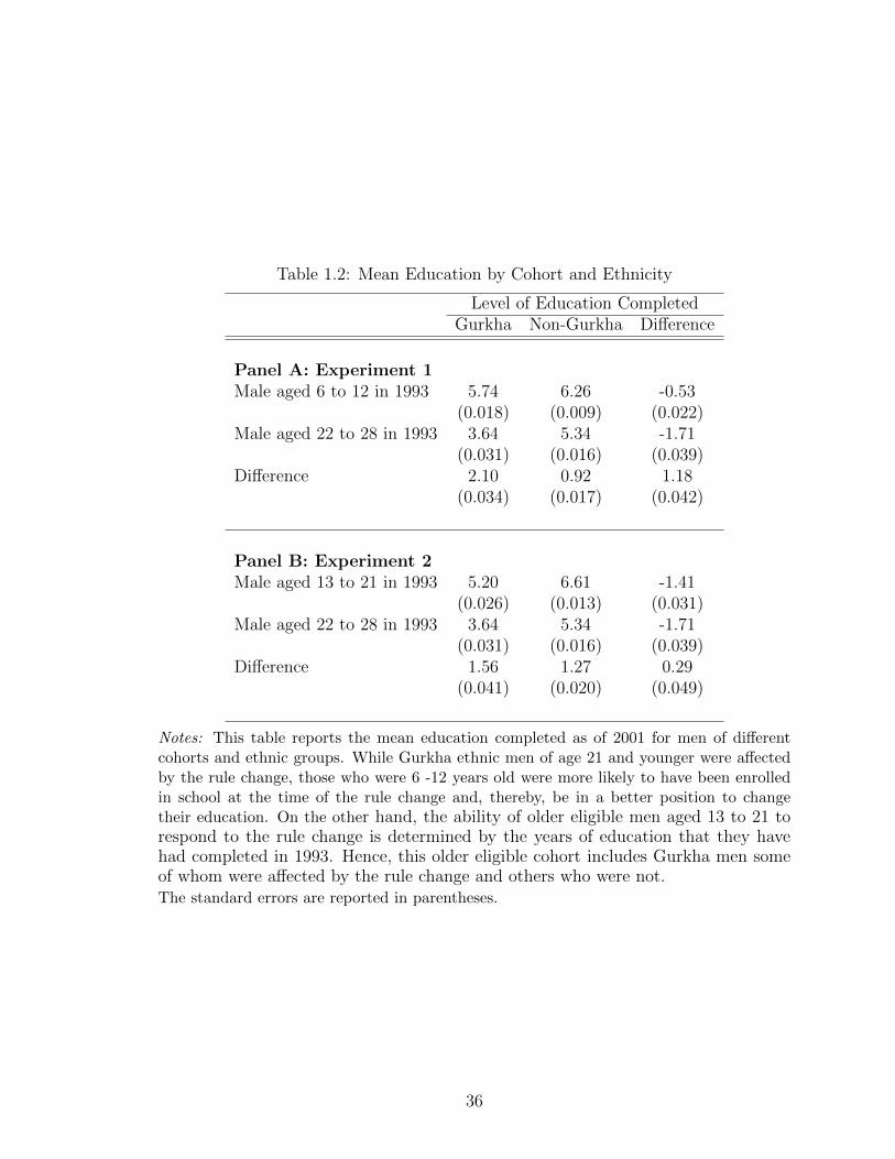
Table 1.2: Mean Education by Cohort and Ethnicity

Level of Education CompletedGurkha Non-Gurkha Di↵erence

Panel A: Experiment 1Male aged 6 to 12 in 1993 5.74 6.26 -0.53

(0.018) (0.009) (0.022)Male aged 22 to 28 in 1993 3.64 5.34 -1.71

(0.031) (0.016) (0.039)Di↵erence 2.10 0.92 1.18

(0.034) (0.017) (0.042)

Panel B: Experiment 2Male aged 13 to 21 in 1993 5.20 6.61 -1.41

(0.026) (0.013) (0.031)Male aged 22 to 28 in 1993 3.64 5.34 -1.71

(0.031) (0.016) (0.039)Di↵erence 1.56 1.27 0.29

(0.041) (0.020) (0.049)

Notes: This table reports the mean education completed as of 2001 for men of di↵erentcohorts and ethnic groups. While Gurkha ethnic men of age 21 and younger were a↵ectedby the rule change, those who were 6 -12 years old were more likely to have been enrolledin school at the time of the rule change and, thereby, be in a better position to changetheir education. On the other hand, the ability of older eligible men aged 13 to 21 torespond to the rule change is determined by the years of education that they havehad completed in 1993. Hence, this older eligible cohort includes Gurkha men someof whom were a↵ected by the rule change and others who were not.The standard errors are reported in parentheses.

36

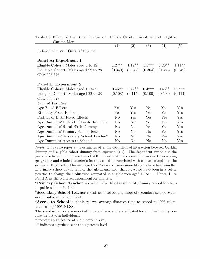
Table 1.3: E↵ect of the Rule Change on Human Capital Investment of EligibleGurkha Men

(1) (2) (3) (4) (5)

Independent Var: Gurkha*Eligible

Panel A: Experiment 1Eligible Cohort: Males aged 6 to 12 1.27** 1.19** 1.17** 1.20** 1.11**Ineligible Cohort: Males aged 22 to 28 (0.340) (0.342) (0.364) (0.386) (0.342)Obs: 325,876

Panel B: Experiment 2Eligible Cohort: Males aged 13 to 21 0.45** 0.42** 0.42** 0.46** 0.39**Ineligible Cohort: Males aged 22 to 28 (0.108) (0.115) (0.100) (0.104) (0.114)Obs: 300,327Control Variables:Age Fixed E↵ects Yes Yes Yes Yes YesEthnicity Fixed E↵ects Yes Yes Yes Yes YesDistrict of Birth Fixed E↵ects No Yes Yes Yes YesAge Dummies*District of Birth Dummies No No Yes Yes YesAge Dummies*Rural Birth Dummy No No Yes Yes YesAge Dummies*Primary School Teachera No No No Yes YesAge Dummies*Secondary School Teacherb No No No Yes YesAge Dummies*Access to Schoolc No No No No Yes

Notes: This table reports the estimates of �, the coe�cient of interaction between Gurkhadummy and eligible cohort dummy from equation (1.4). The dependent variable is theyears of education completed as of 2001. Specifications correct for various time-varyinggeographic and ethnic characteristics that could be correlated with education and bias theestimate. Eligible Gurkha men aged 6 -12 years old were more likely to have been enrolledin primary school at the time of the rule change and, thereby, would have been in a betterposition to change their education compared to eligible men aged 13 to 21. Hence, I usePanel A as the preferred experiment for analysis.aPrimary School Teacher is district-level total number of primary school teachersin pubic schools in 1994.bSecondary School Teacher is district-level total number of secondary school teach-ers in pubic schools in 1994.cAccess to School is ethnicity-level average distance-time to school in 1996 calcu-lated using 1996 NLSS.The standard errors are reported in parentheses and are adjusted for within-ethnicity cor-relation between individuals.* indicates significance at the 5 percent level** indicates significance at the 1 percent level

37

Table 1.4: E↵ect of the Rule Change on Human Capital Investment of IneligibleGurkha Men and Eligible Gurkha Women (Falsification Tests)

(1) (2) (3) (4) (5)


Panel A: Control Experiment 1Eligible Cohort: Males aged 22 to 28 0.23 0.23 -0.02 0.03 0.01Ineligible Cohort: Males aged 29 to 35 (0.213) (0.224) (0.186) (0.176) (0.166)Obs: 214,315

Panel B: Control Experiment 2Eligible Cohort: Males aged 22 to 28 -0.09 -0.06 -0.48 -0.43 -0.62Ineligible Cohort: Males aged 38 to 44 (0.241) (0.428) (0.261) (0.467) (0.466)Obs: 192,046

Panel C: Control Experiment 3Eligible Cohort: Females aged 6 to 12 0.57 0.54 0.12 0.17 -0.09Ineligible Cohort: Females aged 22 to 28 (0.408) (0.407) (0.345) (0.332) (0.351)Obs: 333,055Control Variables:Age Fixed E↵ects Yes Yes Yes Yes YesEthnicity Fixed E↵ects Yes Yes Yes Yes YesDistrict of Birth Fixed E↵ects No Yes Yes Yes YesAge Dummies*District of Birth Dummies No No Yes Yes YesAge Dummies*Rural Birth Dummy No No Yes Yes YesAge Dummies*Primary School Teacher No No No Yes YesAge Dummies*Secondary School Teacher No No No Yes YesAge Dummies*Access to School No No No No Yes

Notes: This table reports the estimates of �, the coe�cient of interaction between Gurkhadummy and eligible cohort dummy from equation (1.4). All three experiments estimate thee↵ect on individuals who were not a↵ected by the rule change. Panel A and B estimatesthe e↵ect on Gurkha men of cohorts, aged 22 to 28. In panel B, the age di↵erence betweenthe two cohorts aged 22 to 28 and aged 38 to 44 is the same as in panel A of Table 1.4.Panel C estimates the e↵ect on Gurkha women of eligible cohort aged 6 to 12. None of theGurkha women were a↵ected because the recruitment of British Gurkha is limited to men.The lack of significant results in these three control experiments provide support for thevalidity of the identification assumption used in Table 1.4 that the di↵erence in educationbetween the cohorts would have been same across Gurkha and non-Gurkha ethnic groupsin the absence of the rule change.* indicates significance at the 5 percent level** indicates significance at the 1 percent level

38

Table 1.5: E↵ect of the Rule Change on Human Capital Investment of EligibleGurkha Men at Each Birth Cohort

(1) (2) (3) (4) (5)

Gurkha*Age 21 -0.30 -0.32 -0.18 -0.14 -0.20(0.162) (0.167) (0.119) (0.120) (0.149)

Gurkha*Age 20 0.21 0.19 0.16 0.18 0.18(0.115) (0.132) (0.119) (0.122) (0.189)

Gurkha*Age 19 0.31* 0.30* 0.32** 0.36** 0.34**(0.104) (0.110) (0.070) (0.062) (0.079)

Gurkha*Age 18 0.20 0.17 0.25* 0.30* 0.27(0.118) (0.121) (0.094) (0.093) (0.142)

Gurkha*Age 17 0.86** 0.85** 0.54* 0.59* 0.40(0.192) (0.188) (0.184) (0.181) (0.188)

Gurkha*Age 16 0.23 0.22 0.31 0.34 0.36(0.186) (0.182) (0.155) (0.163) (0.190)

Gurkha*Age 15 0.50* 0.49* 0.64** 0.69** 0.60**(0.196) (0.203) (0.171) (0.166) (0.181)

Gurkha*Age 14 0.74** 0.71** 0.70** 0.72** 0.56**(0.138) (0.136) (0.161) (0.180) (0.182)

Gurkha*Age 13 0.65** 0.57* 0.65** 0.69** 0.68**(0.200) (0.209) (0.205) (0.218) (0.194)

Gurkha*Age 12 1.13** 1.09** 0.91** 0.95** 0.80**(0.223) (0.220) (0.214) (0.227) (0.213)

Gurkha*Age 11 0.94** 0.86* 0.94** 0.98** 0.81**(0.293) (0.298) (0.281) (0.303) (0.265)

Gurkha*Age 10 1.23** 1.12** 1.01* 1.06** 0.98**(0.224) (0.229) (0.276) (0.297) (0.256)

Gurkha*Age 9 1.08** 1.01* 1.06* 1.09* 1.04*(0.377) (0.373) (0.371) (0.394) (0.351)

Gurkha*Age 8 1.39** 1.27** 1.31** 1.33** 1.25**(0.409) (0.413) (0.405) (0.428) (0.418)

Gurkha*Age 7 1.51** 1.41** 1.38* 1.39* 1.34*(0.454) (0.466) (0.491) (0.513) (0.462)

Gurkha*Age 6 1.39* 1.30* 1.38* 1.38* 1.36*(0.601) (0.598) (0.557) (0.579) (0.541)

Control Variables:District of Birth Fixed E↵ects No Yes Yes Yes YesAge Dummies*District of Birth Dummies No No Yes Yes YesAge Dummies*Rural Birth Dummy No No Yes Yes YesAge Dummies*Primary School Teacher No No No Yes YesAge Dummies*Secondary School Teacher No No No Yes YesAge Dummies*Access to School No No No No Yes

Notes: All specifications include age and ethnicity fixed e↵ects. The standard errors are adjustedfor within-ethnicity correlation between individuals.

39

Table 1.6: E↵ect of the Rule Change on School Enrollment of Young Eligible GurkhaMen (Using Linear Probability Model)

Obs (1) (2) (3) (4) (5)

Extensive Margin

Dep Var: Dummy IndicatingYears of Education >0

325,876 0.12** 0.12** 0.10** 0.10* 0.10*(0.033) (0.034) (0.034) (0.035) (0.034)

Control Variables:Age Fixed E↵ects Yes Yes Yes Yes YesEthnicity Fixed E↵ects Yes Yes Yes Yes YesDistrict of Birth Fixed E↵ects No Yes Yes Yes YesAge Dummies*District of Birth Dummies No No Yes Yes YesAge Dummies*Rural Birth Dummy No No Yes Yes YesAge Dummies*Primary School Teacher No No No Yes YesAge Dummies*Secondary School Teacher No No No Yes YesAge Dummies*Access to School No No No No Yes

Notes: This table reports the estimates of �, the coe�cient of interaction between Gurkhadummy and eligible cohort dummy, from equation (1.4) with a dummy dependent variableindicating the years of education completed greater zero. The sample includes men fromyounger eligible cohorts aged 6 to 12 or ineligible cohort aged 22 to 28. Because prior tothe introduction of educational requirement in 1993 no formal education required to jointhe British Gurkha Army, the above coe�cients estimate the e↵ect of the rule change atthe extensive margin. The standard errors are reported in parentheses and are adjusted forwithin-ethnicity correlation between individuals.* indicates significance at the 5 percent level** indicates significance at the 1 percent level

40

Table 1.7: E↵ect of the Rule Change on Human Capital Investment of Young EligibleGurkha Men (Di↵erential E↵ect)

Whole Distance to Schoola Household Enterpriseb Household Incomec

Sample Median >Median Ag Land No Ag Land Owns TV No TV(1) (2) (3) (4) (5) (6) (7)

1.17** 1.16* 1.18** 0.86* 1.34** 1.29** 0.76**(0.364) (0.416) (0.347) (0.284) (0.391) (0.320) (0.269)

325,879 181,159 144,717 130,698 195,178 86,851 239,025

Notes: This table reports the estimates of �, the coe�cient of interaction between Gurkhadummy and eligible dummy from equation (4). The dependent variable is the years ofeducation completed as of 2001. The sample includes men of eligible cohort aged 6 to 12and ineligible cohort aged 22 to 28. All the columns use specification from column 3 inTable 1.4, which includes ethnicity dummies, age dummies, district of birth dummies, agedummies*district of birth dummies, and age dummies*rural birth dummies.aDistance to School: Sample divided into two categories based on average traveltime to school in 1996: individuals born in (1) districts with average travel time toschool median district-level travel time and (2) districts with average travel timeto school � median district-level travel time. The median district-level travel time toschool is 0.36 hours.bHousehold Enterprise: Sample divided into two categories based on ownership ofagricultural land and livestocks in 2001.cHousehold Income: Sample divided into two categories based on ownership of atelevision set in 2001.The standard errors are reported in parentheses and are adjusted for within-ethnicity cor-relation between individuals.* indicates significance at the 5 percent level** indicates significance at the 1 percent level

41

Table 1.8: E↵ect of the Rule Change on Migration of Eligible Gurkha Men (UsingLinear Probability Model)

(1) (2) (3) (4) (5)

Dependent Var: Dummy IndicatingForeign Residence in 2001

Panel A: Experiment 1Eligible Cohort: Males aged 6 to 12 -0.01 -0.01 -0.01** -0.01** -0.01**Ineligible Cohort: Males aged 22 to 28 (0.004) (0.004) (0.003) (0.003) (0.003)Obs: 325,876Panel B: Experiment 2Eligible Cohort: Males aged 13 to 21 -0.00 -0.00 -0.00 -0.00 -0.00Ineligible Cohort: Males aged 22 to 28 (0.002) (0.002) (0.001) (0.001) (0.001)Obs: 300,327Control Variables:Age Fixed E↵ects Yes Yes Yes Yes YesEthnicity Fixed E↵ects Yes Yes Yes Yes YesDistrict of Birth Fixed E↵ects No Yes Yes Yes YesAge Dummies*District of Birth Dummies No No Yes Yes YesAge Dummies*Rural Birth Dummy No No Yes Yes YesAge Dummies*Primary School Teachera No No No Yes YesAge Dummies*Secondary School Teacherb No No No Yes YesAge Dummies*Access to Schoolc No No No No Yes

Notes: This table reports the estimates of �, the coe�cient of interaction between Gurkhadummy and eligible cohort dummy from equation (4). The dependent variable is the dummyvariable indicating whether the individual is living abroad in 2001. Eligible Gurkha men,especially cohort aged 13 to 21, would have had the opportunity to apply for the BritishGurkha Army by 2001 and also to seek other emigration opportunities. The coe�cients arestatistically insignificant for cohort aged 13 to 21, suggesting that the increase in educationin response to the rule change did not increase their propensity to emigrate. If anything,the emigration is reduced for eligible Gurkha men aged 6 to 12, as suggested by the negativeand statistically significant coe�cients in Panel A.aPrimary School Teacher is district-level total number of primary school teachersin pubic schools in 1994.bSecondary School Teacher is district-level total number of secondary school teach-ers in pubic schools in 1994.cAccess to School is ethnicity-level average distance-time to school in 1996 calcu-lated using 1996 NLSS.The standard errors are reported in parentheses and are adjusted for within-ethnicity cor-relation between individuals.* indicates significance at the 5 percent level** indicates significance at the 1 percent level

42

Table 1.9: E↵ect of the Rule Change on Human Capital Investment of EligibleGurkha Men (Non-Migrants)

(1) (2) (3) (4) (5)


Panel A: Experiment 1Eligible Cohort: Males aged 6 to 12 1.30** 1.22** 1.19** 1.22** 1.14**Ineligible Cohort: Males aged 22 to 28 (0.341) (0.344) (0.366) (0.388) (0.344)Obs: 320,592

Panel B: Experiment 2Eligible Cohort: Males aged 13 to 21 0.45** 0.42** 0.42** 0.46** 0.40**Ineligible Cohort: Males aged 22 to 28 (0.108) (0.116) (0.101) (0.105) (0.114)Obs: 293,946Control Variables:Age Fixed E↵ects Yes Yes Yes Yes YesEthnicity Fixed E↵ects Yes Yes Yes Yes YesDistrict of Birth Fixed E↵ects No Yes Yes Yes YesAge Dummies*District of Birth Dummies No No Yes Yes YesAge Dummies*Rural Birth Dummy No No Yes Yes YesAge Dummies*Primary School Teachera No No No Yes YesAge Dummies*Secondary School Teacherb No No No Yes YesAge Dummies*Access to Schoolc No No No No Yes

Notes: This table reports the estimates of �, the coe�cient of interaction between Gurkhadummy and eligible cohort dummy from equation (4). The dependent variable is the yearsof education completed as of 2001. The sample includes only men who had not emigrated by2001. Specifications correct for various time-varying geographic and ethnic characteristicsthat could be correlated with education and bias the estimate. Eligible Gurkha men, espe-cially cohort aged 13 to 21, would have had the opportunity to apply for the British GurkhaArmy by 2001 and also to seek other emigration opportunities. The positive impact on theeducation of eligible Gurkha men who had not emigrated suggests that the rule change ledto a net increase in the human capital stock of eligible Gurkha men.aPrimary School Teacher is district-level total number of primary school teachersin pubic schools in 1994.bSecondary School Teacher is district-level total number of secondary school teach-ers in pubic schools in 1994.cAccess to School is ethnicity-level average distance-time to school in 1996 calcu-lated using 1996 NLSS.The standard errors are reported in parentheses and are adjusted for within-ethnicity cor-relation between individuals.* indicates significance at the 5 percent level** indicates significance at the 1 percent level

43

Table 1.10: Lifetime Earnings of British Gurkha Soldier

Timeline Income Present Valueof Incomea

1. Recruitment into the British Gurkha at age 20b

New Entrant $20,880.00 $20,880.00Rifleman (Level 1) $26,037.00 $25,776.63Rifleman (Level 2) $28,068.00 $27,509.45Rifleman (Level 3) $31,000.00 $30,079.27Rifleman (Level 4) $33,320.00 $32,007.06Rifleman (Level 5) $36,842.00 $35,036.38Lance Corporal (Level 1) $38,634.00 $36,373.14Lance Corporal (Level 2) $40,407.00 $37,661.96Lance Corporal (Level 3) $42,224.00 $38,961.97Lance Corporal (Level 4) $44,256.00 $40,428.62Lance Corporal (Level 5) $44,256.00 $40,024.33Corporal (Level 1) $44,256.00 $39,624.09Corporal (Level 2) $44,286.00 $39,254.44Corporal (Level 3) $46,454.00 $40,764.36Corporal (Level 4) $47,539.00 $41,299.31Corporal (Level 5) $48,686.00 $41,872.80Corporal (Level 6) $49,694.00 $42,312.34Corporal (Level 7) $50,779.00 $42,803.81Sergeant (Level 1) $50,779.00 $42,375.77Sergeant (Level 2) $51,424.00 $42,484.90Sergeant (Level 3) $52,727.00 $43,125.78Sergeant (Level 4) $53,392.00 $43,232.99Sergeant (Level 5) $54,432.00 $43,634.36Sergeant (Level 6) $55,471.00 $44,022.58Sergeant (Level 7) $56,512.00 $44,400.24

Subtotal $1,092,355.00 $955,946.58

44

Lifetime Earnings of British Gurkha Soldier (Continued)

2. Retirement from British Gurkha at age 45c

(Between age 45 to 65, the pension is calculatedunder Early Departure Payments Structure)

(i) Between 45 to 55:Highest Pensionable Salary*Years of Service*1/70*(50%+8.3335%)=

56512*25*1/70*58.3335%=$11,773.37

x 10= $117,733.67 $87,562.871st Lump Sum = 3 * Pension $35,320.11 $27,472.74

Subtotal $153,053.78 $115,035.61

(ii) Between 55 to 65:Highest Pensionable Salary*Years of Service*1/70*(75%)=

56512*25*1/70*75%=$15,137.14

x10= $151,371.43 $101,815.75

Subtotal $151,371.43 $101,815.75

(After age 65, the pension is calculated under AFPS 05)

(iii) Between age 65 to 75d:Highest Pensionable Salary*Years of Service*1/70=

56512*25*1/70=$20,182.85

x10= $201,828.57 $122,773.762nd Lump Sum = 3 * Pension $60,548.57 $38,520.11

Subtotal $262,377.14 $161,293.87Total $1,659,157.35 $1,334,091.81

Notes: This table reports the lifetime income of a typical Gurkha soldier, including annualsalary, benefits, and pensions.a Present value of income is calculated using a discount factor of 0.99. If income in the thirdyear of service is $28,068, then the present value of third year’s income is 0.992*28,068 =$27,509.45b Salary structure for British Gurkha soldier is based on “Rates of Pay as of April 2009”published by the UK Ministry of Defensec Pension scheme is based on “Armed Forces Pension Scheme 05: Your Pension SchemeExplained” published by Service Personnel Policy (Pensions), The UK Ministry of Defenseon January 2007.

45

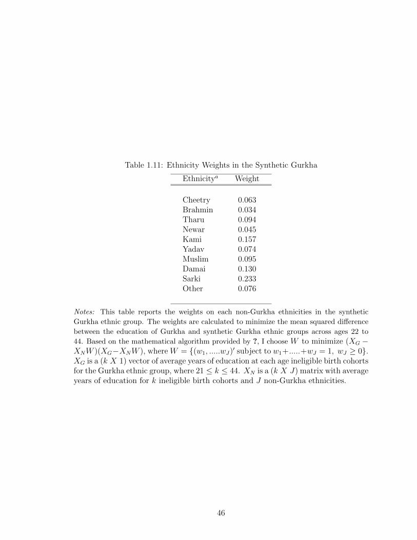
Table 1.11: Ethnicity Weights in the Synthetic Gurkha

Ethnicitya Weight

Cheetry 0.063Brahmin 0.034Tharu 0.094Newar 0.045Kami 0.157Yadav 0.074Muslim 0.095Damai 0.130Sarki 0.233Other 0.076

Notes: This table reports the weights on each non-Gurkha ethnicities in the syntheticGurkha ethnic group. The weights are calculated to minimize the mean squared di↵erencebetween the education of Gurkha and synthetic Gurkha ethnic groups across ages 22 to44. Based on the mathematical algorithm provided by ?, I choose W to minimize (X

G

�X

N

W )(XG

�XN

W ), whereW = {(w1

, .....wJ

)0 subject to w1

+.....+wJ

= 1, wJ

� 0}.X

G

is a (k X 1) vector of average years of education at each age ineligible birth cohortsfor the Gurkha ethnic group, where 21 k 44. X

N

is a (k X J) matrix with averageyears of education for k ineligible birth cohorts and J non-Gurkha ethnicities.

46

CHAPTER II

Sibling Rivalry in Education: Estimation of

Intrahousehold Trade-o↵s in Human Capital

Investment

2.1 Introduction

Households are key decision-makers of their children’s human capital investment,

which is a crucial determinant of their welfare and their country’s economic growth.

Sub-Saharan African countries spent on average 5% of its gross domestic product on

education in 2008.1 Despite this, half of all children still do not complete primary

education in more than one-third of these countries. Improving educational outcomes

for children requires a better understanding of the mechanisms that govern their

households’ investment decisions.

Standard household models developed by Becker (1981) and Newman and Gertler

(1994), identify various factors that a↵ect schooling, one of which is the trade-o↵

among household members. The theoretical model suggests that a child’s educational

outcome could a↵ect the education of other children living in the same household.

An increase in the child’s education shifts resources away from other children in

1The emphasis on education is illustrated by the UN’s Millennium Development Goals (MDGs),where two of the eight goals focus on education–achieve universal primary education and achievegender equality at all levels of education by 2015.

47

the household. It decreases the household’s current income by limiting the child’s

ability to participate in the labor market. While these two mechanisms suggest a

negative trade-o↵ between siblings’ education, it could also have a positive impact

by decreasing the per-child fixed cost of education, increasing the permanent income

of the household, and decreasing the marginal benefit from leisure for other children.

Therefore, an increase in the child’s education can either raise or lower the education

of other children in the household and estimating whether this e↵ect is positive or

negative becomes an empirical question.

The causal estimation of the “inter-sibling” e↵ect in education is, however, con-

strained by endogeneity concerns. Strauss and Thomas (1995) point out that there

are significant unobserved heterogeneity across households that a↵ect their members’

educational outcomes. Hence using the child’s education to estimate its impact on

the education of other children in the household leads to a biased estimate because

unobserved household characteristics are likely to be correlated with the education of

all the children in the household. Moreover, the child’s education a↵ects other chil-

dren’s education and vice versa. Manski (1993) argues that this reflection problem

could lead to a biased estimate of the e↵ect of child’s education on other children

living in the household.

The ideal experiment requires two groups of households from developing countries–

treatment and control households, that are similar in all socio-economic character-

istics. Furthermore, the children in each households are randomly divided into two

groups– targeted and non-targeted children. The targeted children from the treat-

ment household experience an exogenous increase in educational attainment. The

di↵erence in education between the non-targeted children in the treatment household

and the non-targeted children in the control household could be interpreted as the

inter-sibling e↵ect in education.

A unique event occurred in Nepal in 1993 that resembled key aspects of the ideal

48

experiment. The British Gurkha tradition involves an annual recruitment of Nepali

men by the British government into the British Armed Forces. Due to historical

reasons, the majority of British Gurkha soldiers are comprised of 5 out of 15 ethnic

groups of Nepal. These five ethnic groups are of Mongolian-Tibeto origin and are

referred to as the “Gurkha” ethnic group for the remainder of this paper. All the

other ethnic groups are referred to as “non-Gurkha”s.

The natural experiment involves a change in British Gurkha Army recruitment

regulations. In 1993, the British government changed the educational requirement

for the British Gurkha Army applicants, from requiring no education to requiring a

minimum of 8th grade education. The change was prompted by a broader ideological

shift within the British Army regarding the importance of educated and well-trained

soldiers2. As a result, the timing of the change is exogenous to social, economic, or

political characteristics of Nepal and mainly a↵ected the men from the Gurkha ethnic

group who were age eligible to apply to the British Gurkha Army in 1993.

This creates a unique natural experiment in which age eligible men from the

Gurkha ethnic group exclusively experienced an exogenous change in their educa-

tional returns and as a consequence, change in their educational outcomes. More

importantly, since women are ineligible to join the British Gurkha Army, women

of Gurkha ethnic groups were only a↵ected by the rule change through an increase

in the education of age-eligible Gurkha men living in their household. As a conse-

quence, Gurkha females with age eligible male sibling comprise the treatment group;

whereas, the control group includes the Gurkha females who do not have age eligible

male siblings and all non-Gurkha females.

The results suggest that the existence of at least one age eligible male sibling in

the household decreased the education of Gurkha girls by 0.11 years, which implies

a decrease of 7% from their mean education of 1.56 years. Moreover, the results

2“King’s Statement to the Commons on Future Defense Structure.” The Times. July 26, 1990

49

indicate that the estimated negative inter-sibling e↵ect decreases with greater child

spacing, increases with greater number of age eligible male siblings, increases with

household’s involvement in agricultural production, and decreases with more remote

access to school.

The rest of the paper is structured as follows: Section 2 discusses the household

models that highlight the interaction among its members. Section 3 describes the

natural experiment used for causal identification. Section 4 describes the data used

for empirical estimation. Section 5 presents the empirical results. Section 6 presents

robustness for the identification strategy. Section 7 identifies potential mechanisms

that jointly determine the results and Section 8 concludes.

2.2 Previous Literature

The important role of education in fostering long-term economic growth in devel-

oping countries have motivated economists and policymakers to examine how house-

holds could be encouraged to increase their demand for their children’s education.

Angrist and Lavy (1999) use Maimonides rule to determine the class size in Israel

and find that reducing class size had positive impact on test scores of fourth and

fifth graders. Kremer et al. (2009) find that introducing merit based scholarships

for girls in Kenya significantly increased their school attendance and academic exam

scores. They also find positive spillover e↵ects among girls who were unlikely to win

the scholarship and boys who were ineligible for the scholarship. Duflo and Hanna

(2005) find that increasing teacher attendance in India increased student grades and

improved their graduation rate by 62%. Schultz (2004a) suggest that the Progresa

program, a conditional educational grant, in rural Mexico increased education by

10%.

These studies examine the impact of educational policies but ignore the spillover

e↵ect of these policies on non-targeted household members. Angelucci et al. (2009)

50

find that the Progresa program only a↵ected the schooling of secondary school-age

children whose extended household included the primary school-age children receiving

cash transfers. They identify the redistribution of resources within the family net-

work as the main mechanism driving this result. This suggests that the interactions

among household members and the division of resources among them are crucial in

determining how household members respond to various education policies. It also

suggests that education interventions could create spillover e↵ects on non-targeted

household members, which might lead to a over- or under-estimation of the overall

impact of these policies.

The models of household behavior have been critical in identifying numerous mech-

anisms that govern the household decision making process. Household production

models (Becker , 1965; Gronau, 1977; Becker , 1981; Newman and Gertler , 1994) sug-

gest that households maximize their welfare given their resource constraints. One

of the key aspects of these theoretical models is the allocation of time of household

members across various market and non-market activities, including leisure, labor,

home production, and human capital investment.

The division of labor and resources among household members is determined by

the members’ characteristics and market factors. According to Becker (1965, 1981),

household members who are relatively more e�cient at certain activities would also

spend more of their time on those activities compared to other members. This sug-

gests that the household members’ socio-economic choices, which the household has

control over, including human capital investment, are related to observed and unob-

served household characteristics and therefore, should be treated as endogenous.

Bommier and Lambert (2000) find that the di↵erences in male and female marriage

markets in Tanzania could explain the gender based di↵erences in school enrollment

age. They find that households send their daughter to school at a younger age and also

leave school at a younger age than their sons in order to maximize the present value

51

of the bride price. Behrman et al. (1982) find that parents spend more household re-

sources on the children with relatively smaller genetic endowment because they value

their o↵-springs’ earnings equality. These findings underscore the interdependency of

a household member’s socio-economic outcomes with the household preferences and

household members’ characteristics.

The household production model also highlights the trade-o↵s among household

members in socio-economic activities, such as consumption, leisure, and human cap-

ital investment. Becker (1965) points out that an increase in the relative e�ciency

of any member on performing certain activities would result in a reallocation of the

time spent by all other members away from those activities. Newman and Gertler

(1994) find that the time worked on farm by any family member a↵ects the marginal

benefit to farm work for all the family members. They also find that an increase in

the leisure of a member a↵ects the marginal rate of substitution between leisure and

consumption for other household members. These results suggest that the household

members’ choices are interrelated and the interactions among household members are

crucial in determining household outcomes, including its members’ human capital

investment.

Pitt et al. (1990) investigate the e↵ect of child morbidity on the activities of other

household members. They find that an increase in child morbidity in a household

does not a↵ect male siblings but a↵ects mother and female siblings, where the mother

shifts out of labor force into home care and female siblings drop out of school into

the home production. Rosenzweig and Wolpin (1980), Lee (2008), and Qian (2009)

study the e↵ect of an increase in the number of children on the household on child

quality, including human capital investment. Rosenzweig and Wolpin (1980) use twin

births as an exogenous increase in the number of children to find that it has a negative

impact on schooling in rural India. Lee (2008) uses the son preferences and the first

child’s gender to determine that a greater number of siblings have adverse e↵ects on

52

per-child investment in education. Using the relaxation of one child policy in rural

China as an exogenous increase in family size, Qian (2009), on the other hand, finds

that an additional sibling increases school enrollment of the first child by 8-17%.

2.3 Empirical Strategy

The e↵ect of increasing a child’s education on the education choices of other

children in the household is ambiguous. The educational outcome of the other children

is partly governed by the intra-household interactions, triggered by the increase in

education of the child, as suggested by the earlier studies (Becker , 1965; Behrman

et al., 1982; Pitt et al., 1990; Newman and Gertler , 1994; Lee, 2008; Angelucci et al.,

2009; Qian, 2009). Some of the mechanisms, such as the redistribution of household

resources and decrease in household income, suggest a negative impact of increasing a

child’s education on the education of other children; whereas other mechanisms, such

as the lowering of per child fixed costs of schooling, increase in permanent household

income, and the economies of scale in leisure, indicate a positive inter-sibling e↵ect

in education. Hence, an increase in the chid’s education can either raise or lower

the education of other children in the household and estimating whether this e↵ect

is positive or negative becomes an empirical question.

The causal estimation of the inter-sibling e↵ect in education is, however, con-

strained by endogeneity concerns because of the unobserved heterogeneity across

households that are correlated with the education of all their members as indicated by

Strauss and Thomas (1995) and due to the reflection problem highlighted by Manski

(1993). The ideal experiment requires dividing the households with multiple chil-

dren into two random groups– treatment and control households. Furthermore, the

children in only the treatment households are randomly divided into two groups–

treatment and control children. The treatment children in these households are sub-

ject to an exogenous increase in education. Under these circumstances, the di↵erence

53

in the educational attainment between the control children in the treatment house-

holds and the children in the control households could be interpreted as the causal

estimate of the inter-sibling e↵ect in education.

A unique event occurred in Nepal in 1993 that resembled key aspects of the ideal

experiment. It involves a change in the education requirement a↵ecting the recruit-

ment of Nepalese men by the British government into the British Armed Forces.

2.3.1 British Brigade of Gurkha

Nepal is a landlocked country surrounded by India on three sides and China to

its north. Its geographical position historically made it a melting ground for people

and cultures from both north and south of its border (Shrestha, 2001b). The 1996

National Living Standard Survey categorizes the population of Nepal into 15 ethnic

groups. Out of them, the Gurkha ethnic group is comprised of 5 Mongoloid tribal

groups—the Rai, Limbu, Gurung, Magar, and Tamang, who settled in the eastern

and central hills of Nepal during the initial wave of migration from north.

The recruitment of Nepalese men into the British Army started after the Anglo-

Gurkha war (1814-1817). The treaty of Sugauli following the end of the war in 1817

allowed the British to set up three Gurkha regiments in the British Indian Army.

The early recruits included ethnic groups such as the Rajput, Thakuri, Chetri, and

Brahman, who migrated from south and were closely associated with the ethnicities

found in India. In 1857, Indian soldiers serving in the British Indian Army led a

mutiny against the British rule. Although the rebellion was eventually contained in

1858, the British became wary of Indian nationals serving in their army. Rathaur

(2001) and Caplan (1995) argue that as a result, the British also stopped recruiting

Nepalese men belonging to the ethnicities that originated from India into the British

Gurkha Army. According to Rathaur (2001) after 1857, the new Nepali recruits in

the British Gurkha Army were mainly drawn from the Rai, Limbu, Gurung, Magar,

54

and Tamang ethnic groups who, unlike other ethnicities in Nepal, had migrated from

north. This ethnicity bias in the recruitment of the British Gurkha Army continues to

exist till present day as majority of the current British Gurkha soldiers are comprised

of these 5 Mongolian-Tibeto ethnic groups.

The benefits from joining the British Gurkha Army is substantial. The present

value of the lifetime income of serving in the British Gurkha Army for 25 years is

estimated to be about $1,522,750 (Shrestha, 2011). This includes a starting salary

of $21,000 and a lifelong annual pension of about $15,000 after serving for 25 years.

According to Caplan (1995), remittances from Gurkha soldiers and pensions for ex-

Gurkha soldiers were the country’s largest earner of foreign currency until recent

development of tourism and other sources of migration. More importantly, the pay

and pensions of the servicemen are the major source of capital in most Mongolian-

Tibeto communities in the hills of Nepal whose main alternative employment is limited

to farming.3 The financial benefits of British Gurkha Army in these communities is

evident from quotes documented by Caplan (1995) such as, “One of my boys has gone

to the Army, we have only that hope.”

2.3.2 Natural Experiment: A Change in Education Criteria

Education is an important aspect of the selection process. Since 1997, the recruits

must have completed at least 10 years of education. However prior to 1993, no formal

education was required to join the British Gurkha Army. Moreover, the selection

process was strictly limited to physical examinations. In 1993, the British Army

changed its educational requirement and the new Gurkha recruits were required to

have completed at least 8 years of education. Following the change in educational

requirement, mathematics and English grammar tests were added to the selection

3The Defense Committee of the British House of Commons in 1989 suggested that the annualsalary of a British Gurkha soldier was about 100 times the average income in the hills from wherethey come from.

55

process.

The change in educational requirement was a result of a series of defense reviews,

termed “Option for Change,” conducted by the UKMinistry of Defense in early 1990s.

The Option for Change led to an extensive restructuring of the British Armed Forces

in order to cut defense spending after the end of the Cold War. It led to a reduction

in service manpower by 18% to an Army of around 120,0004. More importantly, it

focused on maintaining a leaner, trained, and educated army with better technological

capabilities5.

Since the change in the British Gurkha education requirement was instigated by a

broader restructuring of the British Army, the timing of the change is unlikely to be

correlated to any social, economic, or political characteristics of Nepal at that time.

As a result, this change created an exogenous increase in educational returns abroad

for a subset of individuals in Nepal.

Shrestha (2011) finds that the change in the education requirement to join the

British Gurkha Army led Gurkha men to increase their education by an average of

1.24 years. It induced 19.5 percent of Gurkha men who would not have received

any formal education in the absence of the rule change, to enroll in school. Shrestha

(2011) shows that the impact of the rule change was significant among Gurkha men

of age 12 or younger in 1993, because they were likely to be enrolled in school at

the time of the rule change and also had su�cient number of years to meet the new

educational requirement. Individuals who were 12 or younger in 1993 are referred to

as “age-eligible” for the remainder of this paper.

4The Eighth Defense Report published by the Defense Committee, House of Commons in 1997.5The shift towards better-educated soldiers in 1990s was not unique to the British Army but

was also prevalent in the US Army. According to the Tenth Quadrennial Review of US MilitaryCompensation, the number of recruits with high school diploma increased by 30% in mid-1980s andthose who scored better than the median in the Armed Forces Qualification Test (AFQT) increasedby 10% in early 1990s

56

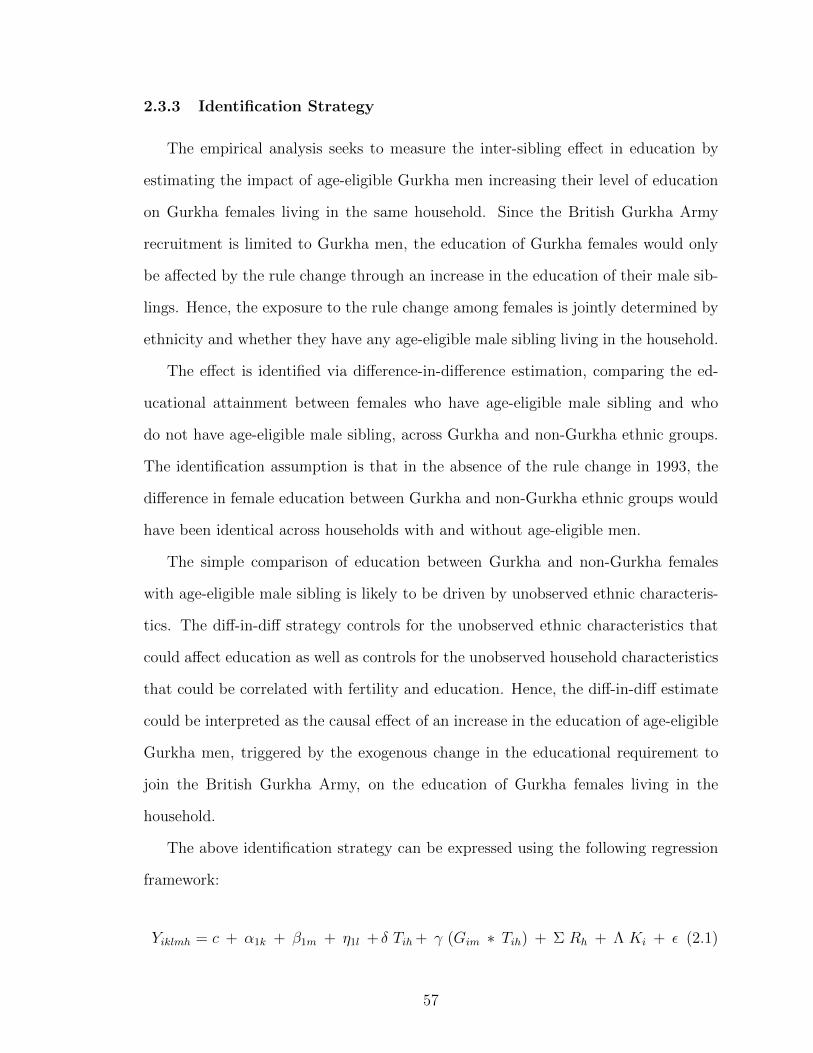
2.3.3 Identification Strategy

The empirical analysis seeks to measure the inter-sibling e↵ect in education by

estimating the impact of age-eligible Gurkha men increasing their level of education

on Gurkha females living in the same household. Since the British Gurkha Army

recruitment is limited to Gurkha men, the education of Gurkha females would only

be a↵ected by the rule change through an increase in the education of their male sib-

lings. Hence, the exposure to the rule change among females is jointly determined by

ethnicity and whether they have any age-eligible male sibling living in the household.

The e↵ect is identified via di↵erence-in-di↵erence estimation, comparing the ed-

ucational attainment between females who have age-eligible male sibling and who

do not have age-eligible male sibling, across Gurkha and non-Gurkha ethnic groups.

The identification assumption is that in the absence of the rule change in 1993, the

di↵erence in female education between Gurkha and non-Gurkha ethnic groups would

have been identical across households with and without age-eligible men.

The simple comparison of education between Gurkha and non-Gurkha females

with age-eligible male sibling is likely to be driven by unobserved ethnic characteris-

tics. The di↵-in-di↵ strategy controls for the unobserved ethnic characteristics that

could a↵ect education as well as controls for the unobserved household characteristics

that could be correlated with fertility and education. Hence, the di↵-in-di↵ estimate

could be interpreted as the causal e↵ect of an increase in the education of age-eligible

Gurkha men, triggered by the exogenous change in the educational requirement to

join the British Gurkha Army, on the education of Gurkha females living in the

household.

The above identification strategy can be expressed using the following regression

framework:

Yiklmh

= c + ↵1k

+ �1m

+ ⌘1l

+ � Tih

+ � (Gim

⇤ Tih

) + ⌃ Rh

+ ⇤ Ki

+ ✏ (2.1)

57

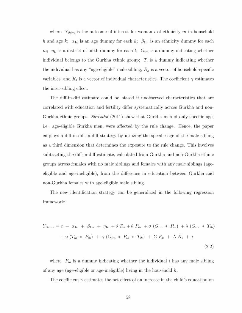
where Yiklm

is the outcome of interest for woman i of ethnicity m in household

h and age k; ↵1k

is an age dummy for each k; �1m

is an ethnicity dummy for each

m; ⌘1l

is a district of birth dummy for each l; Gim


individual belongs to the Gurkha ethnic group; Ti


the individual has any “age-eligible” male sibling; Rh

is a vector of household-specific

variables; and Kl

is a vector of individual characteristics. The coe�cient � estimates

the inter-sibling e↵ect.

The di↵-in-di↵ estimate could be biased if unobserved characteristics that are

correlated with education and fertility di↵er systematically across Gurkha and non-

Gurkha ethnic groups. Shrestha (2011) show that Gurkha men of only specific age,

i.e. age-eligible Gurkha men, were a↵ected by the rule change. Hence, the paper

employs a di↵-in-di↵-in-di↵ strategy by utilizing the specific age of the male sibling

as a third dimension that determines the exposure to the rule change. This involves

subtracting the di↵-in-di↵ estimate, calculated from Gurkha and non-Gurkha ethnic

groups across females with no male siblings and females with any male siblings (age-

eligible and age-ineligible), from the di↵erence in education between Gurkha and

non-Gurkha females with age-eligible male sibling.

The new identification strategy can be generalized in the following regression

framework:

Yiklmh

= c + ↵1k

+ �1m

+ ⌘1l

+ � Tih

+ ✓ Pih

+ � (Gim

⇤ Pih

) + � (Gim

⇤ Tih

)

+ ! (Tih

⇤ Pih

) + � (Gim

⇤ Pih

⇤ Tih

) + ⌃ Rh

+ ⇤ Ki

+ ✏

(2.2)

where Pih

is a dummy indicating whether the individual i has any male sibling

of any age (age-eligible or age-ineligible) living in the household h.

The coe�cient � estimates the net e↵ect of an increase in the child’s education on

58

the education of other children living in the household, which is jointly determined by

numerous o↵-setting mechanisms. On one hand, an increase in the child’s education

shifts resources away from the education of other children in the household. It also

limits the child’s ability to participate in the labor market which decreases the current

income of the household. On the other hand, it has a positive impact by decreasing

the per child fixed cost of education, by increasing the permanent income of the

household, and by decreasing the marginal benefit of leisure for other children.

2.4 Data

The paper uses the data from 2001 Census of Nepal. The empirical analysis

focuses on females who were 6 years old to 12 years old in 2001. The census data

are supplemented with 1996 Nepal Living Standards Surveys (NLSS), which is a

household sample survey with greater detail. Table 2.1 presents summary statistics

for the 235,297 girls from the 2001 Census as well as the 3,373 households from the

1996 NLSS.

Individual and household level averages for some socio-economic characteristics

are provided for the entire sample as well as separately for the Gurkha and non-

Gurkha ethnic groups. The Gurkha ethnic group comprises of just under 20 percent

of the samples in both surveys. Panel A shows that the average level of education

for the Gurkha ethnic group is 1.53, which is slightly lower than the average for the

non-Gurkha ethnic group of 1.59. Similarly, 79.3% of Gurkha girls were born in rural

area compared to 64% of non-Gurkha girls. 65% of Gurkha girls have age-eligible

male sibling compared to 65.7% of non-Gurkha girls. The average household size

for Gurkha and no-Gurkha ethnic groups are 6.16 and 6.30 respectively. Panel B

suggests that near the time of the rule change, non-Gurkha households had better

access to school facilities, health clinics, and transportation than Gurkha households.

48.5% of Gurkha households were living in poverty compared to 46.9% of non-Gurkha

59

households.

2.5 Results

The di↵-in-di↵ strategy compares the educational attainment of females who have

at least one age-eligible male sibling in the household to those who do not have

any age-eligible male sibling, in both Gurkha and non-Gurkha ethnic groups. Table

2.2 shows average years of education completed as of 2001 for females of age 6 to

12 in 2001.The empirical analysis focuses on girls 6 to 12 years old for three main

reasons. First, they are of similar age compared to men who were a↵ected by the rule

change, and as a result are most likely to complete with age-eligible men for household

resources including human capital investment. Second, they are old enough to have

the opportunity to enroll in school by 2001 and have data on education. Third, they

are young enough to be not married in 2001 and hence, have information on male

siblings who grew up with them6.

The results in table 2.2 show that an average education for Gurkha girls with

age-eligible male sibling is 1.62 years, which is less compared to non-Gurkha girls

with age-eligible male sibling whose average education is 1.72 years. This di↵erence

of 0.09 years is statistically significant at the 5 percent level. On the other hand,

among girls with no age-eligible male sibling7, there is no statistical di↵erence in the

average education across Gurkha and non-Gurkha ethnic groups. This suggests that

in the absence of the rule change, the female educational attainment would not have

di↵ered across Gurkha and non-Gurkha ethnic groups, even among girls with age-

eligible male siblings. The simple di↵erence-in-di↵erences estimation shows that girls

6The information on male siblings is obtained from the household roster. As a result, if a womengets married and moves into a new household with her spouse before 2001, then the household rosteronly provides information of the members living with her in 2001 but not the members who she grewup with before she got married. Among girls of age 6 to 12 in 2001, 0.7% are married and as aresult, are dropped from the empirical analysis.

7The sample of girls with no age-eligible male sibling includes females who have no male siblingor who have only age-ineligible male siblings.

60

of Gurkha ethnic group with at least one age-eligible male sibling completed 0.11 less

years of education. This is significantly di↵erent from zero at the 1% level.

Table 2.3 presents the di↵erence-in-di↵erence strategy by estimating coe�cient �

in equation (2.1) for dependent variable– years of education completed as of 2001.

The specification in column 1 does not control for any individual and household char-

acteristics and hence, the di↵-in-di↵ estimate is identical to the estimate of table 2.2.

The specification in column 2, on the other hand, controls for cohort of birth dummies

and ethnicity dummies because the di↵erence in age distribution and ethnicity com-

position of girls with and without age-eligible male siblings, might not be consistent

across Gurkha and non-Gurkha ethnic groups. The estimates in column 2 suggest

that education of Gurkha girls with age-eligible male siblings decreased by 0.09 years,

which implies a decrease of 6% from a mean education of 1.56 years. The estimate is

statistically significant at the 1% level.

Figure 2.1 shows that Gurkha ethnic group is concentrated in the mid-north and

north-east districts of Nepal. Table 2.1, panel A suggests that girls from Gurkha

ethnic groups are less likely to be born in an urban region than non-Gurkha girls.

Since the regional characteristics could be correlated with fertility and education,

the specification in columns 3, 4, 5, and 6 includes district of birth dummies and a

dummy indicating whether a girl was born in a rural region. The estimate in column

3 do not change and remains statistically significant at the 1% level.

Table 2.1 also suggests that among girls who have at least one age-eligible male

sibling, Gurkha girls are likely to have slightly more number of age-eligible male

siblings than non-Gurkha girls. The unobserved characteristics that are correlated

with fertility and education could be di↵erent across Gurkha and non-Gurkha ethnic

groups. The specification in columns 4, 5, and 6 controls for the household size, the

number of age-eligible male siblings, and the number of male siblings of any age;

whereas the specification in columns 5 and 6 additionally controls for age spacing

61

between the girl and her age-eligible male sibling as well as age gap between her and

her male sibling of any age. The results in columns 4 and 5 suggest that having any

age-eligible men in the household decreased Gurkha girls education by 0.09 years.

This implies that an increase in educational returns for age-eligible Gurkha men

reduced Gurkha girls education by 6%, from an average education of 1.56 years of

completed schooling in 2001.

The specification in column 6 corrects for other ethnic characteristics, such as

access to school, access to healthcare, and poverty. These ethnic-level characteristics

are obtained from 1996 NLSS. The estimates in column 6 are also statistically signif-

icant at the 1% level and suggest that an exogenous increase in the the educational

returns of age-eligible Gurkha men decreased education of Gurkha girls living in the

same household by 0.08 years.

The above interpretation is based on the assumption in the absence of the rule

change, the di↵erence in education between Gurkha and non-Gurkha girls would

have been identical across households with and without age-eligible men. The results

in table 2.1, however, suggest that unobserved ethnic characteristics could be jointly

correlated with fertility and education. Table 2.4 corrects for these unobserved ethnic

characteristics by employing a di↵-in-di↵-in-di↵ strategy and estimating coe�cient �

in equation (2.2).

Table 2.4 presents the estimates for two dependent variables and 6 di↵erent spec-

ifications similar to table 2.3. The estimates in all the columns of table 2.4 do not

change considerably compared to the estimates in table 2.3 and are statistically sig-

nificant at the conventional levels. The results in column 5 suggest that an increase in

educational returns for age-eligible Gurkha men decreased the education of Gurkha

girls with age-eligible male sibling by 0.11 years. The results indicate that an inter-

sibling e↵ect of human capital investment is likely to be negative.

62

2.6 Robustness

The validity of the empirical strategy relies on the assumption that fertility is

una↵ected by the change in educational requirement. Since fertility is measured

through household roster, the interpretation of the above results as an inter-sibling

e↵ect of education requires that the change in the educational requirement of the

British Gurkha Army in 1993 did not a↵ect the number of individuals, especially

male siblings, living together in the household among Gurkha ethnic group.

The change in the British Gurkha Army education requirement in 1993 could

induce age-eligible or age-ineligible Gurkha men to leave the household. The data on

number of male siblings living separately from the household is available for a subset

of girls used in the empirical analysis. The subsample for whom the information

regarding the number of male siblings living separately is available, includes 97.5%

of Gurkha girls and 96.2% of non-Gurkha girls from the original sample.

Table 2.5 and table 2.6 estimates coe�cient � in equation (2.1) and (2.2) respec-

tively for this subsample. In both tables, specification in columns 2, 5, and 6 includes

a dummy indicating whether the girl has a male sibling living separately from the

household. The results in table 2.5 and 2.6 indicate that controlling for male siblings

who are not part of the household in 2001 does not change the estimates in any of the

specifications. More importantly, the estimates in columns 2, 4, and 6 in table 2.5

and 2.6 are all statistically significant at the conventional level. This suggests that

the results in table 2.3 and 2.4 can not be explained thought the changes in house-

hold structure of Gurkha ethnic group, mainly the departure of male siblings from

the household triggered by the rule change in 1993, but are more likely to be driven

by the intra-household sibling interactions induced by the increase in educational

attainment among age-eligible male siblings living in the household.

The departure of male siblings from the household also implies that they are not

counted as the girl’s male siblings in the empirical analysis. If unobserved ethnic

63

characteristics are correlated with education and the likelihood of having all age-

eligible male siblings living separately, then the above results are likely to be biased.

Table 2.7 compares the household composition between Gurkha and non-Gurkha

ethnic groups. The results in table 2.7 show that both Gurkha and non-Gurkha

girls are equally likely to have at least one age-eligible male sibling living in the

household, suggesting the absence of di↵erential household formation across the two

ethnic groups. Moreover, figure 2.2 suggests that age-eligible male siblings, who are

20 years old or younger in 2001, are too young to live separately from their parents.

According to figure 2.2, only 1.94% of Gurkha households are headed by men of age

20 or younger and 2.24% of non-Gurkha households are headed by age-eligible men.

Table 2.8 employs an alternate strategy to assess household formation bias. Columns

1 and 2 presents the triple di↵erence estimates from table 2.6, columns 1 and 3 re-

spectively. The specification in columns 3 and 4 assumes that all the male siblings

living separately in 2001 belong to the age-ineligible cohort and more importantly,

they would have lived in the same household as the girl in the absence of the rule

change. The results in columns 3 and 4 suggest that including male siblings living

separately as age-ineligible male siblings living in the household for all girls in the

subsample, does not change the estimates compared to columns 1 and 2. Similarly,

the specification in columns 5 and 6 assumes that all the male siblings living sep-

arately in 2001 belong to the age-eligible cohort and would have lived in the same

household as the girl if not for the rule change. Under this assumption, the estimates

in columns 5 and 6 of inter-sibling e↵ect does not di↵er from the estimates in columns

1 and 2 and are also statistically significant at the 1% level. This suggests that the

negative results in table 2.3 and 2.4 are not likely to be driven by di↵erential attrition

of male siblings from the household.

Finally, the paper employs a placebo study to examine whether the results could

be explained by unobserved ethnic characteristics that are correlated with education

64

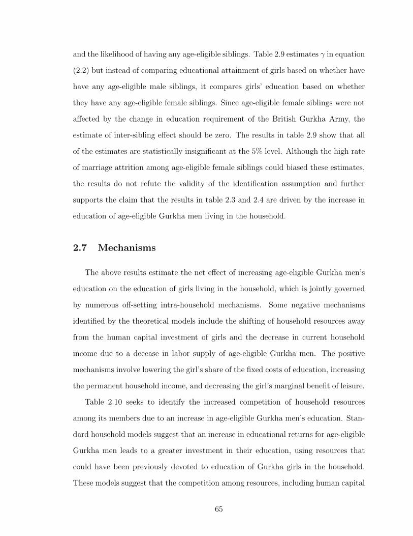
and the likelihood of having any age-eligible siblings. Table 2.9 estimates � in equation

(2.2) but instead of comparing educational attainment of girls based on whether have

have any age-eligible male siblings, it compares girls’ education based on whether

they have any age-eligible female siblings. Since age-eligible female siblings were not

a↵ected by the change in education requirement of the British Gurkha Army, the

estimate of inter-sibling e↵ect should be zero. The results in table 2.9 show that all

of the estimates are statistically insignificant at the 5% level. Although the high rate

of marriage attrition among age-eligible female siblings could biased these estimates,

the results do not refute the validity of the identification assumption and further

supports the claim that the results in table 2.3 and 2.4 are driven by the increase in

education of age-eligible Gurkha men living in the household.

2.7 Mechanisms

The above results estimate the net e↵ect of increasing age-eligible Gurkha men’s

education on the education of girls living in the household, which is jointly governed

by numerous o↵-setting intra-household mechanisms. Some negative mechanisms

identified by the theoretical models include the shifting of household resources away

from the human capital investment of girls and the decrease in current household

income due to a decease in labor supply of age-eligible Gurkha men. The positive

mechanisms involve lowering the girl’s share of the fixed costs of education, increasing

the permanent household income, and decreasing the girl’s marginal benefit of leisure.

Table 2.10 seeks to identify the increased competition of household resources

among its members due to an increase in age-eligible Gurkha men’s education. Stan-

dard household models suggest that an increase in educational returns for age-eligible

Gurkha men leads to a greater investment in their education, using resources that

could have been previously devoted to education of Gurkha girls in the household.

These models suggest that the competition among resources, including human capital

65

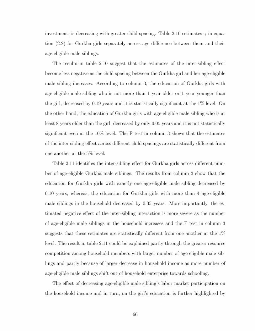
investment, is decreasing with greater child spacing. Table 2.10 estimates � in equa-

tion (2.2) for Gurkha girls separately across age di↵erence between them and their

age-eligible male siblings.

The results in table 2.10 suggest that the estimates of the inter-sibling e↵ect

become less negative as the child spacing between the Gurkha girl and her age-eligible

male sibling increases. According to column 3, the education of Gurkha girls with

age-eligible male sibling who is not more than 1 year older or 1 year younger than

the girl, decreased by 0.19 years and it is statistically significant at the 1% level. On

the other hand, the education of Gurkha girls with age-eligible male sibling who is at

least 8 years older than the girl, decreased by only 0.05 years and it is not statistically

significant even at the 10% level. The F test in column 3 shows that the estimates

of the inter-sibling e↵ect across di↵erent child spacings are statistically di↵erent from

one another at the 5% level.

Table 2.11 identifies the inter-sibling e↵ect for Gurkha girls across di↵erent num-

ber of age-eligible Gurkha male siblings. The results from column 3 show that the

education for Gurkha girls with exactly one age-eligible male sibling decreased by

0.10 years, whereas, the education for Gurkha girls with more than 4 age-eligible

male siblings in the household decreased by 0.35 years. More importantly, the es-

timated negative e↵ect of the inter-sibling interaction is more severe as the number

of age-eligible male siblings in the household increases and the F test in column 3

suggests that these estimates are statistically di↵erent from one another at the 1%

level. The result in table 2.11 could be explained partly through the greater resource

competition among household members with larger number of age-eligible male sib-

lings and partly because of larger decrease in household income as more number of

age-eligible male siblings shift out of household enterprise towards schooling.

The e↵ect of decreasing age-eligible male sibling’s labor market participation on

the household income and in turn, on the girl’s education is further highlighted by

66

the results in table 2.12. Table 2.12 examines the di↵erential inter-sibling interaction

in the education of Gurkha girls based on various socio-economic characteristics, in-

cluding access to schooling and operation of household agricultural enterprise. Since

most of the child labor are limited to household agricultural production, this implies

that households that operate agricultural production experience a greater reduction

in household income as age-eligible Gurkha men devote more of their time on school-

ing and away from household activities. The results in columns 6 and 7 indicate that

education of Gurkha girls with at least one age-eligible male siblings living in the

household that operates agricultural enterprise decreased by 0.12 years and statisti-

cally significant at the 10% level; whereas, for those living in the household that are

not involved in agricultural production decreased by only 0.07 years, which is not

statistically significant at the 10% level. The F stat, however, suggests that these two

estimates are not statistically di↵erent from one another at the conventional level.

The results in table 2.12 also show that the estimated inter-sibling e↵ect is less

negative for households that are in the districts with remote access to school, measured

in terms of average distance-time between the household and the school. Although

the estimates in column 4 and 5 are not statistically di↵erent from one another at

the 10% level, it does suggests that the ability to spread fixed cost of transport

across multiple siblings (including girls) moderates the negative e↵ect of having an

age-eligible brother, but does not overturn it8.

2.8 Conclusion

Education has been the focal point of development policies for the past few

decades. Economist and policymakers alike have devoted significant resources on

8Although the fixed cost of schooling has multi-facets, the empirical analysis is focused on onlyone aspect of the fixed cost, i.e. time it takes to drop and pick up children to and from school. Thedistricts with more remote access to school indicates a large fixed cost of sending children to schoolas parents have to devote more time transporting their children to school.

67

understanding and evaluating household’s response to various educational policy in-

terventions. Since households are the key decision makers of their children’s educa-

tional outcomes, it is important to investigate these educational policies in the context

of household decision-making process.

Although theoretical household behavior models highlight the interactions among

household members regarding various socio-economic decisions, including human cap-

ital investment, the empirical estimation of how the education of one child a↵ects the

education of other children living in the household is absent due to endogeneity con-

cerns. The paper utilized a unique natural experiment involving an increase in the

educational requirement to join the British Gurkha Army for age eligible Gurkha

men, to estimate the e↵ect on the education of Gurkha girls living in the same house-

hold as them. Although the triple di↵erence estimation suggests a robust negative

inter-sibling e↵ect, the result should be considered carefully given the unique nature

of the British Gurkha recruitment, which is unlike any other labor markets or policy

interventions.

The paper sought to identify some of the o↵-setting mechanisms that govern the

inter-sibling interaction in education, including resource competition among its mem-

bers, changes in household income, and sharing of the fixed cost of schooling. How-

ever, a more suitable natural experiment or a well-designed randomized control trial

is required to precisely estimate the magnitudes of each of these mechanisms that

jointly determine the inter-sibling e↵ect in education.

The paper highlights the importance of inter-sibling interactions in determining

the socio-economic outcomes of its household members. It suggests a need to under-

stand these interactions not only in educational outcomes but also other important

variables such as health, nutrition, marriage, fertility, migration, and occupational

choice. Analyzing these socio-economic decisions as a culmination of interactions be-

tween household members’ preferences, choices, and resources, would not only help

68

properly evaluate existing policy interventions but also help formulate more e↵ective

future policies.

69

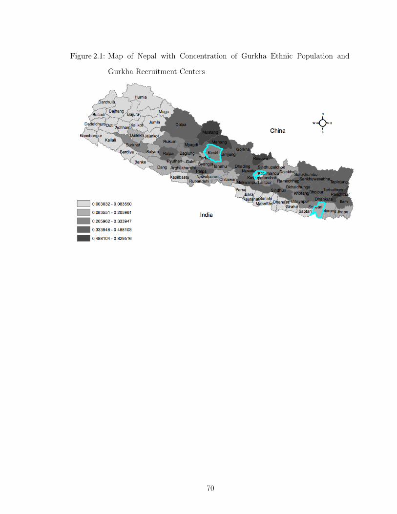
Figure 2.1: Map of Nepal with Concentration of Gurkha Ethnic Population and

Gurkha Recruitment Centers

70

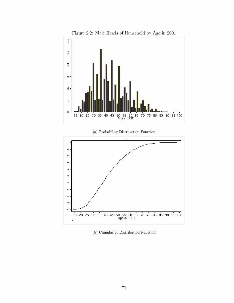
Figure 2.2: Male Heads of Household by Age in 2001

0.0

1.0

2.0

3.0

4.0

5.0

6

15 20 25 30 35 40 45 50 55 60 65 70 75 80 85 90 95 100Age in 2001

(a) Probability Distribution Function

0.1

.2.3

.4.5

.6.7

.8.9

1

15 20 25 30 35 40 45 50 55 60 65 70 75 80 85 90 95 100Age in 2001

kernel = epanechnikov, degree = 0, bandwidth = .28

Local polynomial smooth

(b) Cumulative Distribution Function

71

Table 2.1: Descriptive StatisticsWhole Sample Gurkha Non-Gurkha

Panel A: Individual Level Means2001 Census of Nepal

Total Sample 235,297 44,250 191,047% of sample – 18.8% 81.2%Level of Education 1.58 1.53 1.59Percent Born in Rural 66.9% 79.3% 64.0%Percent Married 0.7% 0.2% 0.8%Age in 2001 8.97 8.99 8.97Household Size 6.27 6.16 6.30Number of Brothers 1.11 1.11 1.10Number of Treated Brothers 1.00 1.01 1.00Percent having Brother(s) 68.4% 67.6% 68.6%Percent having Treated Brother(s) 65.6% 65.0% 65.7%Percent Owning Land 75.5% 82.4% 73.8%Percent Owning Livestock 72.0% 80.6% 70.0%

Panel B: Household Level Means1996 NLSS

Total Sample 3373 544 2829% of Sample – 16.1% 83.9%Access to School 0.38 Hrs 0.54 Hrs 0.35 HrsAccess to Health Post 1.20 Hrs 1.85 Hrs 1.07 HrsAccess to Paved Road 9.30 Hrs 14.45 Hrs 8.30 HrsAnnual Consumption $151.21 $149.93 $151.45Percent of Household in Poverty 33.5% 48.5% 46.9%

72

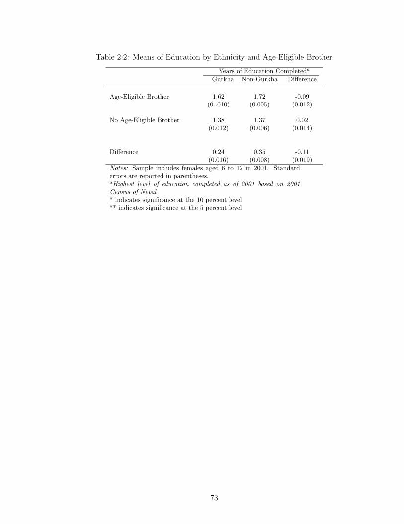
Table 2.2: Means of Education by Ethnicity and Age-Eligible Brother

Years of Education Completeda

Gurkha Non-Gurkha Di↵erence

Age-Eligible Brother 1.62 1.72 -0.09(0 .010) (0.005) (0.012)

No Age-Eligible Brother 1.38 1.37 0.02(0.012) (0.006) (0.014)

Di↵erence 0.24 0.35 -0.11(0.016) (0.008) (0.019)

Notes: Sample includes females aged 6 to 12 in 2001. Standarderrors are reported in parentheses.aHighest level of education completed as of 2001 based on 2001Census of Nepal* indicates significance at the 10 percent level** indicates significance at the 5 percent level

73

Table 2.3: E↵ect of the Rule Change on Human Capital Investment of Gurkha Girlswith Age-Eligible Brother (Di↵erence-in-Di↵erence)

Dependent Variable (1) (2) (3) (4) (5) (6)

Years of Education -0.11** -0.09** -0.09** -0.09** -0.09** -0.08**(0.053) (0.035) (0.040) (0.039) (0.040) (0.037)

No. of Obs 231,777 231,777 229,915 229,915 229,915 225,388

Control Variables:Age Fixed E↵ects No Yes Yes Yes Yes YesEthnicity Fixed E↵ects No Yes Yes Yes Yes YesDistrict of Birth Fixed E↵ects No No Yes Yes Yes YesRural No No Yes Yes Yes YesHousehold Size No No No Yes Yes YesNo. of Brothersa No No No Yes Yes YesNo. of Age-Eligible Brothersb No No No Yes Yes YesBrother Age Di↵ Dummiesc No No No No Yes YesAge-Eligible Brother Age Di↵ Dummiesd No No No No Yes YesAccess to Schoole No No No No No YesAccess to Healthf No No No No No YesPovertyg No No No No No YesNotes: Sample includes females of age 6 to 12 in 2001. Standard errors are reported in parentheses.Standard errors are adjusted for within-caste correlation.a No. of Brothers is a variable indicating the number of brothers living in the household.b No. of Age-Eligible Brothers is a variable indicating the number of treated males living in thehousehold.c Brother Age Di↵ Dummies are dummies indicating the age di↵erence between the individualand her closest brother.d Age Eligible Brother Age Di↵ Dummies are dummies indicating the age di↵erence betweenthe individual and her closest treated brother.eAccess to School is district-level average distance-time to school in 1996 calculated using 1996NLSSfAccess to Health is district-level average distance-time to health post in 1996 calculated using1996 NLSSgPoverty is district-level average household consumption in 1996 calculated using 1996 NLSS* indicates significance at the 10 percent level** indicates significance at the 5 percent level

74

Table 2.4: E↵ect of the Rule Change on Human Capital Investment of Gurkha Girlswith Age-Eligible Brother (Di↵erence-in-Di↵erence-in-Di↵erence)


Years of Education -0.23** -0.14** -0.11* -0.11* -0.11* -0.12**(0.080) (0.063) (0.060) (0.061) (0.060) (0.062)

No. of Obs 231,777 231,777 229,915 229,915 229,915 225,388

Control Variables:Age Fixed E↵ects No Yes Yes Yes Yes YesEthnicity Fixed E↵ects No Yes Yes Yes Yes YesDistrict of Birth Fixed E↵ects No No Yes Yes Yes YesRural No No Yes Yes Yes YesHousehold Size No No No Yes Yes YesNo. of Brothersa No No No Yes Yes YesNo. of Age-Eligible Brothersb No No No Yes Yes YesBrother Age Di↵ Dummiesc No No No No Yes YesAge-Eligible Brother Age Di↵ Dummiesd No No No No Yes YesAccess to Schoole No No No No No YesAccess to Healthf No No No No No YesPovertyg No No No No No YesNotes: Sample includes females of age 6 to 12 in 2001. Standard errors are reported in parentheses.Standard errors are adjusted for within-caste correlation.a No. of Brothers is a variable indicating the number of brothers living in the household.b No. of Age-Eligible Brothers is a variable indicating the number of treated males living in thehousehold.c Brother Age Di↵ Dummies are dummies indicating the age di↵erence between the individualand her closest brother.d Age Eligible Brother Age Di↵ Dummies are dummies indicating the age di↵erence betweenthe individual and her closest treated brother.eAccess to School is district-level average distance-time to school in 1996 calculated using 1996NLSSfAccess to Health is district-level average distance-time to health post in 1996 calculated using1996 NLSSgPoverty is district-level average household consumption in 1996 calculated using 1996 NLSS* indicates significance at the 10 percent level** indicates significance at the 5 percent level

75

Table 2.5: E↵ect of the Rule Change on Human Capital Investment of Gurkha Girlswith Age-Eligible Brother Controlling for Separated Brother (Di↵erence-in-Di↵erence)


Years of Education -0.09** -0.09** -0.09** -0.09** -0.09** -0.09**Obs: 226,075 (0.040) (0.040) (0.039) (0.039) (0.038) (0.038)

Control Variablesa:Separate Brother b No Yes No Yes No YesHousehold Size No No Yes Yes Yes YesNo. of Brothersc No No Yes Yes Yes YesNo. of Age-Eligible Brothersd No No Yes Yes Yes YesBrother Age Di↵ Dummiesc No No No No Yes YesAge-Eligible Brother Age Di↵ Dummiesd No No No No Yes YesNotes: Sample includes females of age 6 to 12 in 2001 for whom data on number of brothers livingseparately from the household are available. The data is available for females whose parents orgrandparents are heads of the household. It comprises of 96% of the sample. Standard errors arereported in parentheses. Standard errors are adjusted for within-correlation.aAll specifications include age fixed e↵ects, ethnicity fixed e↵ects, district of birth fixed e↵ects, andrural dummy.b Separate Brother is a dummy indicating whether the individual has brother(s) living separately.c No. of Brothers is a variable indicating the number of brothers living in the household.d No. of Age-Eligible Brothers is a variable indicating the number of treated males living in thehousehold.* indicates significance at the 10 percent level** indicates significance at the 5 percent level

76

Table 2.6: E↵ect of the Rule Change on Human Capital Investment of Gurkha Girlswith Age-Eligible Brother Controlling for Separated Brother (Di↵erence-in-Di↵erence-in-Di↵erence)


Years of Education -0.21** -0.21** -0.21** -0.21** -0.20** -0.20**Obs: 226,075 (0.066) (0.066) (0.066) (0.066) (0.067) (0.067)

Control Variablesa:Separate Brother b No Yes No Yes No YesHousehold Size No No Yes Yes Yes YesNo. of Brothersc No No Yes Yes Yes YesNo. of Age-Eligible Brothersd No No Yes Yes Yes YesBrother Age Di↵ Dummiesc No No No No Yes YesAge-Eligible Brother Age Di↵ Dummiesd No No No No Yes YesNotes: Sample includes females of age 6 to 12 in 2001 for whom data on number of brothers livingseparately from the household are available. The data is available for females whose parents orgrandparents are heads of the household. It comprises of 96% of the sample. Standard errors arereported in parentheses. Standard errors are adjusted for within caste-correlation.aAll specifications include age fixed e↵ects, ethnicity fixed e↵ects, district of birth fixed e↵ects, andrural dummy.b Separate Brother is a dummy indicating whether the individual has brother(s) living separately.c No. of Brothers is a variable indicating the number of brothers living in the household.d No. of Age-Eligible Brothers is a variable indicating the number of treated males living in thehousehold.* indicates significance at the 10 percent level** indicates significance at the 5 percent level

77

Table 2.7: E↵ect of the Rule Change on the Probability of Having Age-EligibleBrother (Using Linear Probability Model)Dependent Variable (1) (2) (3) (4) (5)

Dummy Indicating -0.00 -0.01 0.00 -0.00 -0.00Age-Eligible Brother(s) (0.011) (0.012) (0.009) (0.008) (0.009)

No. of Obs 231,777 231,777 231,777 231,777 227,213

Control Variables:Age Fixed E↵ects No Yes Yes Yes YesDistrict of Birth Fixed E↵ects No No Yes Yes YesRural No No No Yes YesAccess to School No No No No YesAccess to Health No No No No YesPoverty No No No No YesNotes: Sample includes females of age 6 to 12 in 2001. Standard errorsare reported in parentheses. Standard errors are adjusted for within-castecorrelation.* indicates significance at the 10 percent level** indicates significance at the 5 percent level

78

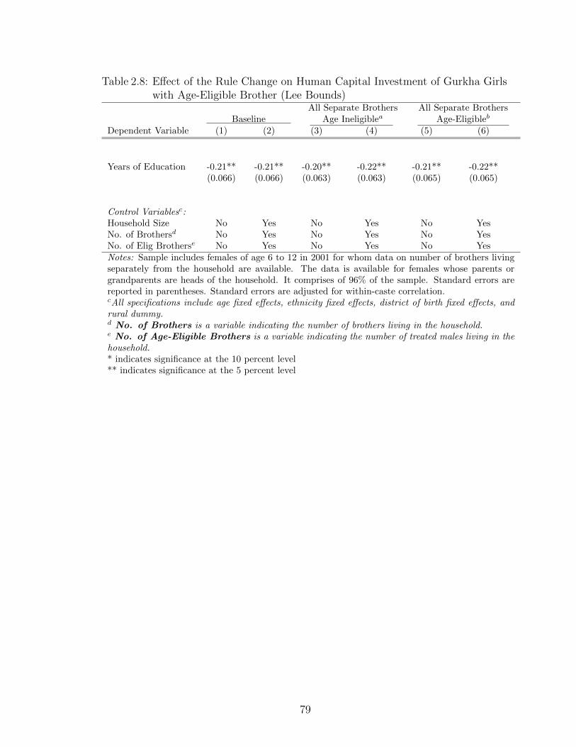
Table 2.8: E↵ect of the Rule Change on Human Capital Investment of Gurkha Girlswith Age-Eligible Brother (Lee Bounds)

All Separate Brothers All Separate BrothersBaseline Age Ineligiblea Age-Eligibleb


Years of Education -0.21** -0.21** -0.20** -0.22** -0.21** -0.22**(0.066) (0.066) (0.063) (0.063) (0.065) (0.065)

Control Variablesc:Household Size No Yes No Yes No YesNo. of Brothersd No Yes No Yes No YesNo. of Elig Brotherse No Yes No Yes No YesNotes: Sample includes females of age 6 to 12 in 2001 for whom data on number of brothers livingseparately from the household are available. The data is available for females whose parents orgrandparents are heads of the household. It comprises of 96% of the sample. Standard errors arereported in parentheses. Standard errors are adjusted for within-caste correlation.cAll specifications include age fixed e↵ects, ethnicity fixed e↵ects, district of birth fixed e↵ects, andrural dummy.d No. of Brothers is a variable indicating the number of brothers living in the household.e No. of Age-Eligible Brothers is a variable indicating the number of treated males living in thehousehold.* indicates significance at the 10 percent level** indicates significance at the 5 percent level

79

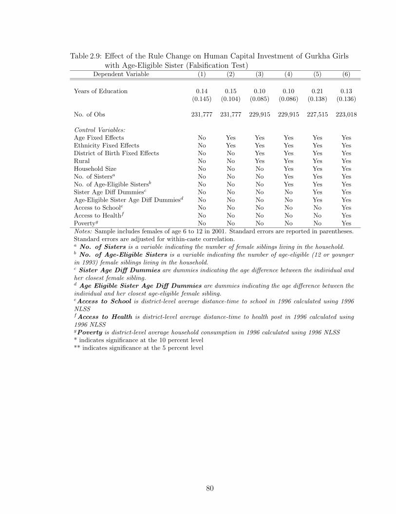
Table 2.9: E↵ect of the Rule Change on Human Capital Investment of Gurkha Girlswith Age-Eligible Sister (Falsification Test)


Years of Education 0.14 0.15 0.10 0.10 0.21 0.13(0.145) (0.104) (0.085) (0.086) (0.138) (0.136)

No. of Obs 231,777 231,777 229,915 229,915 227,515 223,018

Control Variables:Age Fixed E↵ects No Yes Yes Yes Yes YesEthnicity Fixed E↵ects No Yes Yes Yes Yes YesDistrict of Birth Fixed E↵ects No No Yes Yes Yes YesRural No No Yes Yes Yes YesHousehold Size No No No Yes Yes YesNo. of Sistersa No No No Yes Yes YesNo. of Age-Eligible Sistersb No No No Yes Yes YesSister Age Di↵ Dummiesc No No No No Yes YesAge-Eligible Sister Age Di↵ Dummiesd No No No No Yes YesAccess to Schoole No No No No No YesAccess to Healthf No No No No No YesPovertyg No No No No No YesNotes: Sample includes females of age 6 to 12 in 2001. Standard errors are reported in parentheses.Standard errors are adjusted for within-caste correlation.a No. of Sisters is a variable indicating the number of female siblings living in the household.b No. of Age-Eligible Sisters is a variable indicating the number of age-eligible (12 or youngerin 1993) female siblings living in the household.c Sister Age Di↵ Dummies are dummies indicating the age di↵erence between the individual andher closest female sibling.d Age Eligible Sister Age Di↵ Dummies are dummies indicating the age di↵erence between theindividual and her closest age-eligible female sibling.eAccess to School is district-level average distance-time to school in 1996 calculated using 1996NLSSfAccess to Health is district-level average distance-time to health post in 1996 calculated using1996 NLSSgPoverty is district-level average household consumption in 1996 calculated using 1996 NLSS* indicates significance at the 10 percent level** indicates significance at the 5 percent level

80

Table 2.10: Di↵erential E↵ect of the Rule Change on Human Capital Investment ofGurkha Girls with Age-Eligible Brother (By Age Di↵erence)

(1) (2) (3) (4) (5) (6)

0 AgeDiff 1 -0.27** -0.22** -0.19** -0.18** -0.17** -0.20**(0.083) (0.075) (0.075) (0.071) (0.073) (0.076)

2 AgeDiff 3 -0.24** -0.15** -0.12** -0.11* -0.11* -0.12**(0.082) (0.058) (0.059) (0.057) (0.057) (0.057)

4 AgeDiff 5 -0.23** -0.13* -0.11 -0.10 -0.10 -0.11(0.090) (0.068) (0.065) (0.063) (0.063) (0.065)

6 AgeDiff 7 -0.25** -0.15* -0.13* -0.12* -0.12* -0.14**(0.080) (0.074) (0.073) (0.070) (0.070) (0.071)

8 AgeDiff 14 -0.11 -0.07 -0.05 -0.05 -0.05 -0.07(0.113) (0.098) (0.093) (0.091) (0.091) (0.094)

Prob � F(All Coe�cients Equal) 0.412 0.004 0.004 0.003 0.003 0.003

Control Variables:Treated Brother Age Di↵ Dummies Yes Yes Yes Yes Yes YesAge Fixed E↵ects No Yes Yes Yes Yes YesEthnicity Fixed E↵ects No Yes Yes Yes Yes YesDistrict of Birth Fixed E↵ects No No Yes Yes Yes YesRural No No No Yes Yes YesHousehold Size No No No No Yes YesNo. of Brothers No No No No Yes YesNo. of Treated Brothers No No No No Yes YesAccess to School No No No No No YesAccess to Health No No No No No YesPoverty No No No No No YesNotes: Sample includes females of age 6 to 12 in 2001. The dependent variableis the years of education completed as of 2001. Standard errors are reported inparentheses. Standard errors are adjusted for within-caste correlation.* indicates significance at the 10 percent level** indicates significance at the 5 percent level

81

Table 2.11: Di↵erential E↵ect of the Rule Change on Human Capital Investmentof Gurkha Girls with Age-Eligible Brother (By Number of Age-EligibleBrothers)

(1) (2) (3) (4) (5) (6)

No. of Treated Brother = 1 -0.22** -0.13* -0.10 -0.09 -0.09 -0.10*(0.085) (0.064) (0.065) (0.061) (0.061) (0.062)

No. of Treated Brother = 2 -0.25** -0.15** -0.13** -0.12** -0.12** -0.14**(0.076) (0.065) (0.063) (0.061) (0.061) (0.061)

No. of Treated Brother = 3 -0.16 -0.17* -0.16** -0.15* -0.15** -0.17**(0.105) (0.091) (0.080) (0.076) (0.076) (0.079)

No. of Treated Brother � 4 -0.28** -0.36** -0.35** -0.32** -0.32** -0.34**(0.122) (0.101) (0.101) (0.095) (0.095) (0.096)

Prob � F(All Coe�cients Equal) 0.105 0.006 0.010 0.009 0.008 0.007

Control Variables:No. of Treated Brother Dummies Yes Yes Yes Yes Yes YesAge Fixed E↵ects No Yes Yes Yes Yes YesEthnicity Fixed E↵ects No Yes Yes Yes Yes YesDistrict of Birth Fixed E↵ects No No Yes Yes Yes YesRural No No No Yes Yes YesHousehold Size No No No No Yes YesNo. of Brothers No No No No Yes YesAccess to School No No No No No YesAccess to Health No No No No No YesPoverty No No No No No YesNotes: Sample includes females of age 6 to 12 in 2001. The dependent variableis the years of education completed as of 2001. Standard errors are reported inparentheses. Standard errors are adjusted for within-caste correlation.* indicates significance at the 10 percent level** indicates significance at the 5 percent level

82

Table 2.12: Di↵erential E↵ect of the Rule Change on Human Capital Investment ofGurkha Girls with Age-Eligible Brother (By Density, Distance to School,and Operation of Household Enterprise)

Whole Densitya Distance to Schoolb Household Enterprisec

Sample Rural Urban Median � Median Ag Land No Ag Land(1) (2) (3) (4) (5) (6) (7)

-0.12** -0.10 -0.21* -0.15* -0.07 -0.12* -0.07(0.055) (0.064) (0.109) (0.083) (0.075) (0.062) (0.122)

231,777 155,362 76,415 129,734 102,043 152,472 74,741Notes: Sample includes females of age 6 to 12 in 2001. The dependent variable is the years ofschooling completed as of 2001. Standard errors are reported in parentheses. Standard errors areadjusted for within-caste correlation. All specifications include age fixed e↵ects, ethnicity fixede↵ects, district of birth fixed e↵ects, rural dummy, and household size.a Density: Sample divided into two categories based on population density in the area of birth:individuals born in rural area and urban area.b Distance to School: Sample divided into two categories based on average distance-time to schoolin 1996: individuals born in districts with average distance-time to school median district-leveltime and districts with average distance-time to school � median district-level time. The mediandistrict-level distance-time to school is 0.36 hours.c Household Enterprise: Sample divided into two categories based on ownership of agriculturalland and livestocks: individuals in household with agricultural land and livestocks and household withno agricultural land and no livestocks.* indicates significance at the 10 percent level** indicates significance at the 5 percent level

83

CHAPTER III

Access to the North-South Roads and Farm

Profits in Rural Nepal

3.1 Introduction

Rural transportation is an important development strategy in low-income coun-

tries. It enhances economic gains for agrarian households by providing easier access

to both input and output markets. Moreover, such gains are likely to have a sub-

stantial impact on poverty reduction because the poor are concentrated in the rural

agricultural sector, where transportation infrastructure is most scarce.1

The World Bank in 2005 invested more than $8 billion US dollars on infrastruc-

ture in developing countries, which accounts for 35 percent of their total lending

(World Bank, 2006). But measuring economic benefits of these large investments

is di�cult because of reverse causality. Although past economic growths are often

always accompanied by rapid expansion of infrastructure, such strong correlations

do not imply that investments on infrastructure will promote growth. On one hand,

comparing regions with various degrees of infrastructure could overestimate its e↵ect

on economic development because development in and of itself also increases demand

150 percent of the poor in Nepal live in rural areas and are involved in agricultural production.Rural areas are often characterized by rugged terrain, sparse population, and isolation, therebymaking e↵ective transportation infrastructure for market integration even more crucial.

84

for infrastructure. On the other hand, given Burgess and Jedwab (2010) find that

political appointees considerably influence road allocation across region, if political

power and economic wealth are negatively correlated, this will bias the estimate of

the e↵ect of infrastructure towards zero. I overcome the endogeneity bias by utilizing

a unique geographic feature that exogenously determines the placement of road in

rural Nepal and estimate the impact on its agricultural economy.

Nepal is one of the poorest countries in the world with a dominant agriculture

sector and a sparse road network due to an extremely rugged terrain. Based on 2001

Nepal census data, 44 percent of its population including 3.3 million poor live in the

hills, out of which 75 percent of them rely on agriculture for their livelihoods. The

rough terrain poses a serious challenge for road construction, which is reflected by

one of the lowest road densities in the world.2 Nevertheless, in the last four decades

the government constructed 15,308 kilometers of roads by relying significantly on

international donors, expanding from a meager length of 376 km in 1951.3

The main purpose of these roads is to connect district headquarters, which are

historical fort towns that currently serve as administrative centers. The govern-

ment’s 20-Year Road Plan in 2001 adopted five main objectives, the top of which

was “strengthening political and administrative linkages.” Shrestha (2001a) points

out that the economic consideration is always secondary to the administrative con-

sideration in constructing rural roads. More importantly, because all mountains in

the region span north-south, it is cheaper to construct a north-south road, which

follows one of such mountain ranges, relative to constructing an east-west road that

2In 2007, the road density in Nepal was 121 km/100 km2 or 0.8 km per 1,000 people. Only 43percent of the rural population have access to all-season road and the average distance to the nearesttransportation stop in rural area is 30 kilometers. 60 percent have access to roads within two-hourswalking distance, while 23 percent are beyond a four-hour walk.

3According to the World Bank, Nepal’s road network annually increased by 6.7% between 1995and 2004 with the largest expansion occurring in roads classified as district or rural roads, whichgrew annually by 11% during this period. Based on the “Twenty Year Road Plan” published bythe Ministry of Physical Planning and Work, Department of Roads, the public road expenditureaccounted for 12 percent of the total national budget in 2001.

85

has to cross multiple mountains via bridges.4 This unique geographic feature has

resulted in a road network that includes a single east-west highway that stretches

the entire country and multiple north-south roads, which connect to this highway at

various locations. Each north-south road connects several district headquarters that

are situated directly north of its junction with the east-west highway.

I use this geographic north-south corridors to construct an instrumental variable

to deal with the endogeneity issue of where the road is constructed. In particular, I

divide the country into 10 equal north-south blocks and connect all the district head-

quarters within each block with its nearest district headquarter by using a straight

line.5 Dividing the country into such north-south blocks ensures that the district

headquarters are connected along the north-south direction rather than east-west

direction, as suggested by the geographic feature of mountains. I also connect the

district headquarter that is closest to the east-west highway within each block to that

highway via a shortest distance, which results in 10 north-south lines connecting all

the district headquarters in the hills to the east-west highway. Although 10 north-

south blocks are based on the actual political and administrative division of Nepal,6 I

repeat the algorithm using 12 north-south blocks and show that the results are robust

to my choice of the algorithm parameter. Lastly, I show that the distance to these

straight lines is a strong predictor of household’s proximity to road. Moreover, the

construction of the straight lines are based on two factors, administrative integration

and geographic feature that favors north-south linkages, both of which are likely to

4In 2001, the cost of constructing two-lane bridge in the hill region was estimated to be half amillion rupees per meter. In the same year, the construction of bridges comprised of more than 30percent of the total government funding on road development, and 15 percent of the total road in-vestments based on the estimates from the Ministry of Finance. This illustrates that the constructionof bridges constitutes a significant cost burden on any road project’s total budget.

5As seen in figures 3.3 and 3.5, the following algorithm leads to some district headquarters beingconnected to multiple other district headquarters because the nearest district headquarter pairs arenot symmetric i. e. the district headquarter that is nearest to another district headquarter doesnot always imply that the later district headquarter is also the nearest district headquarter of theformer.

6Nepal is divided into 5 political and administrative regions, as shown in figure 3.4. The fivepairs of these adjoining north-south blocks coincide well with these 5 administrative regions.

86

be independent of the socio-economic characteristics of households in the hinterlands.

My empirical method improves the identification strategies used by previous stud-

ies. While Banerjee et al. (2009) and Atack et al. (2009) construct a straight line

connecting important historical cities to predict modern railway network, their in-

struments coincide with historical trade corridors and therefore could be correlated

with unobserved characteristics that are associated with living close to a historical

route. In contrast, I confine the linkage to a north-south direction making it less

likely to be correlated with historical trade routes, which stretch in both an east-west

and a north-south directions according to Stiller (1976).7 Jacoby and Minten (2008)

include transportation costs directly into a nonparametric model, while arguing that

the di↵erences in transportation costs are due to geographic terrain. The costs are

significantly higher at the top of the mountain relative to the bottom. However, ele-

vation could be correlated with land productivity as well as household’s unobserved

characteristics, especially if poor households are more likely to settle at higher ele-

vations due to cheaper access to those lands. Apart from the physical feature of the

terrain, my empirical strategy also relies on an administrative integration policy to

explain the variation in access to road, and therefore, allows for appropriate controls

of terrain quality such as elevation and land gradient.

Using cross-sectional household data from 2011 Nepal Living Standard Survey

and geo-spatial data from MENRIS, I estimate a 2SLS model to calculate the ef-

fect of roads on household profit from agriculture as measured by the farm value.

If farms behave like assets,8 the improvement in farm’s future profits due to lower

transportation cost should be reflected in its value. This approach is used by Arnott

and Stiglitz (1981) and Jacoby (2000) to circumvent the daunting task of calculating

7Based on Stiller (1976) and Shrestha (2001a), communications between district headquarterswere historically carried out through foot trails that stretched east-west as well as north-south byconnecting the district headquarters via a shortest distance, and they constituted the central nerveof the hill economy prior to the construction of roads.

8The standard asset-pricing model states that the present value of a plot is equal to the discountedsum of its future profits. This hypothesis is tested on rented farm plots later in the paper.

87

actual farm profits. Household surveys in low-income countries lack accurate infor-

mation on farm profits, partly because many input purchases and sales of output are

conducted informally through non-monetary transfers.

My results suggest that decreasing a household’s travel time to the nearest road

by one percent increases its farm value by 0.25 percent. The 2SLS estimates are sta-

tistically significant at the 5 percent level and are robust to the algorithm parameters

used to construct the line. While earlier infrastructure studies like Michaels (2008)

and Donaldson (2010) focus on price convergence from the view point of trade frame-

work, I estimate household-specific economic gains from infrastructure investments.

Because most of the world’s poor inhabit rural areas and agriculture accounts for a

significant fraction of a rural economy, the results directly contribute towards the gov-

ernment’s goal to reduce poverty. Mansuri et al. (2012b) and Mansuri et al. (2012a)

find that farm productivity and commercialization are two important determinants of

escaping poverty in rural Pakistan and Uganda, both of which are likely to be directly

a↵ected by access to transportation (Fafchamps and Hill , 2005; Gollin and Rogerson,

2010). These results are consistent with my findings and together they highlight the

benefits of rural transportation investments on agriculture, poverty alleviation, and

food security.

The rest of the paper is structured as follows: Section 2 describes the geographic

feature that influences road network in Nepal. Section 3 presents a theoretical model

that illustrates the benefits of road projects on farm profits. Section 4 explains the

identification used for causal estimation and Section 5 describes the data used for this

strategy. Section 5 presents the empirical results and Section 7 concludes.

3.2 Background

Nepal is a landlocked country with isolated, localized economies referred to by

Shrestha and Jain (1977) as “pocket economies”. This fragmentation is a direct

88

manifestation of its extremely rugged terrain, which has seriously undermined the

development of adequate communication and transportation infrastructure (Shrestha,

2004). 77 percent of its land surface is covered by mountains and hills, with an

exception of the Terrai plain in the south. The elevation in the hill region changes

sharply from only 80 meters above sea level to more than 8800 meters within a

stretch of just 100 kilometers, making road construction very di�cult. As a result,

road density is only 14 km/100 km2 or 0.8 km per 1,000 people, which is one of the

lowest in the world (Meyer , 2008). Figure 3.1 illustrates the rough landscape that

covers almost the entire country.

Despite such rugged terrain, almost half of the population live in the hills where

poverty incidence of 35 percent is the highest among all the regions (NLSS, 2004).

According to Upadhyaya (2010), majority of these poor own small, fragmented land-

holdings and rely on subsistence farming for their livelihoods.9 Moreover, most of the

hill lands are steeply sloped, highly vulnerable to soil erosion, and impervious to irri-

gation, leading to an extremely low farm productivity (UNDP, 2002). These factors,

together with a poor access to input and output markets due to sparse road network,

severely restrict the economic gains from farming and worsen the food security prob-

lem in the region.10 Therefore, the government has emphasized the construction of

roads in the hill region as an important means to fight poverty.11

One of such infrastructure projects is the construction of the East West Highway

(EWH), which began in the late 1950s but was only completed in the early 2000s.

EWH spans the entire country along its southern border with India in the Terrai

plain, with the total length of 1024 kilometers. It is the longest and the most impor-

946 percent of the land owning households in the hills own less than 0.5 hectare of agriculturalland.

10Based on the estimates by the International Fund for Agricultural Development (IFAD), morethan 48 percent of children under 5 years of age are malnourished in the rural areas of Nepal.

11The Government of Nepal’s Interim Three Year Plan (2007-2010) strongly emphasizes the role ofroads in reducing poverty in rural areas, by improving rural access and prompting higher agriculturaloutput as well as non-farm income in remote hill areas of the country.

89

tant highway in Nepal. According to Shrestha (2004), it is the backbone of Nepal’s

road network and plays a significant role in fostering social, economic, and political

integration, by connecting all the major regional economies.

Although expanding the road network is an important government strategy for

poverty reduction, its chief purpose is geared towards administrative integration by

stressing the linkage between district headquarters. These are historical fort towns,

which are scattered throughout the hill tops, and were converted into administra-

tive centers under the current political system. According to Shrestha (2001a), the

economic consideration have and still remains secondary to the administrative consid-

eration in determining the construction of rural highways. The national transporta-

tion policy of the government states that “high priority shall be given to completing

north-south roads connecting all 75 district headquarters to the main highway.”

3.2.1 North-South Road

North-South (NS) roads are the most cost e↵ective way of connecting district

headquarters due to a geographic feature of the region, especially after the comple-

tion of EWH. All mountain ranges in the hill region span north-south followed by

deep and narrow valleys or rivers on either sides. Consequently, a rural road is con-

structed by following one of such mountains from north to south until the road joins

EWH in the Terrai plain. In contrast to constructing roads that stretch east-west,

NS roads cross fewer mountain ranges and therefore require fewer number of bridges,

which significantly reduces costs. Based on figures from the Finance Ministry, bridge

construction accounts for more than 30 percent of the government’s funding on road

projects and 15 percent of its total road expenditure, which suggests that building

a bridge constitutes a significant cost burden on a project’s budget. Therefore, dis-

trict headquarters are connected to the national road network via NS roads that all

feed into EWH. The Twenty Year Road Plan published by the Ministry of Physical

90

Planning, emphasizes the construction of NS roads and highlights the government’s

reliance on NS roads to achieve its goal of administrative integration.

Transportation and communications between district headquarters were histor-

ically carried out through numerous foot trails that stretch east-west as well as

north-south, connecting the district headquarters via a shortest distance (Stiller ,

1976). Figure 3.2 shows all the foot trails that span across the country. According

to Shrestha (2001a), the network of walking paths across the hills consisted of rope

bridges, ferries, and other means of crossing between mountain ranges and prior to

EWH, they constituted the central nerve of the hill economy. This implies that the

recently constructed NS roads are likely to be uncorrelated with these foot trails that

formed the trade link between district headquarters in the past. More importantly,

the construction of NS roads in order to connect the district headquarters to EWH

led to an exogenous increase in access to road for villages in north-south hinterlands

relative to those in east-west hinterlands.

3.3 Theory

Farmers cultivate a single crop using two factors of production, x kg per hectare

of chemical fertilizer and l hours per hectare of labor. Using a fixed technology,

their crop yield y (kg per hectare) is given by the neoclassical production function

y = f ( x, l ). All farmers trade agricultural output and fertilizer in a competitive

market centers located at the juncture of a rural road and the main highway.12 The

transportation of goods between farms and their nearest market center involves two

components– head-loading goods between the farm and the road using human porters

and trucking goods along the road, the former constituting the majority share of the

12As explained in the earlier section, the road network in Nepal comprises of EWH, which runsthrough the entire country, with various NS roads feeding into this main highway from the north atvarious locations along its length.

91

total transportation cost.13

From a given farm, it takes h hours to reach the nearest road junction and the

portage cost of goods is t Rupees/ (kg hours). If k and p be the prices of fertilizers

and outputs in the market center, respectively, then the e↵ective purchase price of

fertilizer is ek = k + th Rupees/kg and the e↵ective selling price of output is

ep = p � th Rupees/kg.14 Let w be the wage rate of agricultural work. The per

hectare land rent, r, can be defined as the maximal profit that can be earned from a

hectare of land,

r (w, ek, ep ) ⌘ maxl,x

( epy � wl � ekx ) (3.1)

Moreover, using the envelope theorem, the relationship between land rent and

travel time to the nearest road is given by:

d r(w,ek, ep)d h

= �t(y + x) < 0 (3.2)

The above equation implies that an improved access to roads for farmers increases

their agricultural profit and therefore, raises the per hectare rent (r) of their plots.

The negative rent gradient is equal to the total portage cost per hour per hectare.

3.4 Empirical Strategy

While the theoretical analysis above is framed in terms of land rents that capture

the economic profits from cultivation, I use plot values in the empirical analysis

13This feature is likely to closely match the reality on the ground for most rural farmers in thehills, where almost six million people or 23% of the population still live more than four hours’ walkaway from the closest road. The markets at intermediate points between the farms and the road arean inessential complication because goods still need to be head-loaded from the road junction, thecost of which will be reflected on their prices at these intermediate market centers.

14The price of goods, k and p, are assumed not to vary across the market centers along the mainhighway (EWH). However, this assumption is relaxed in the empirical analysis with the inclusion ofdistrict (regional) fixed e↵ects.

92

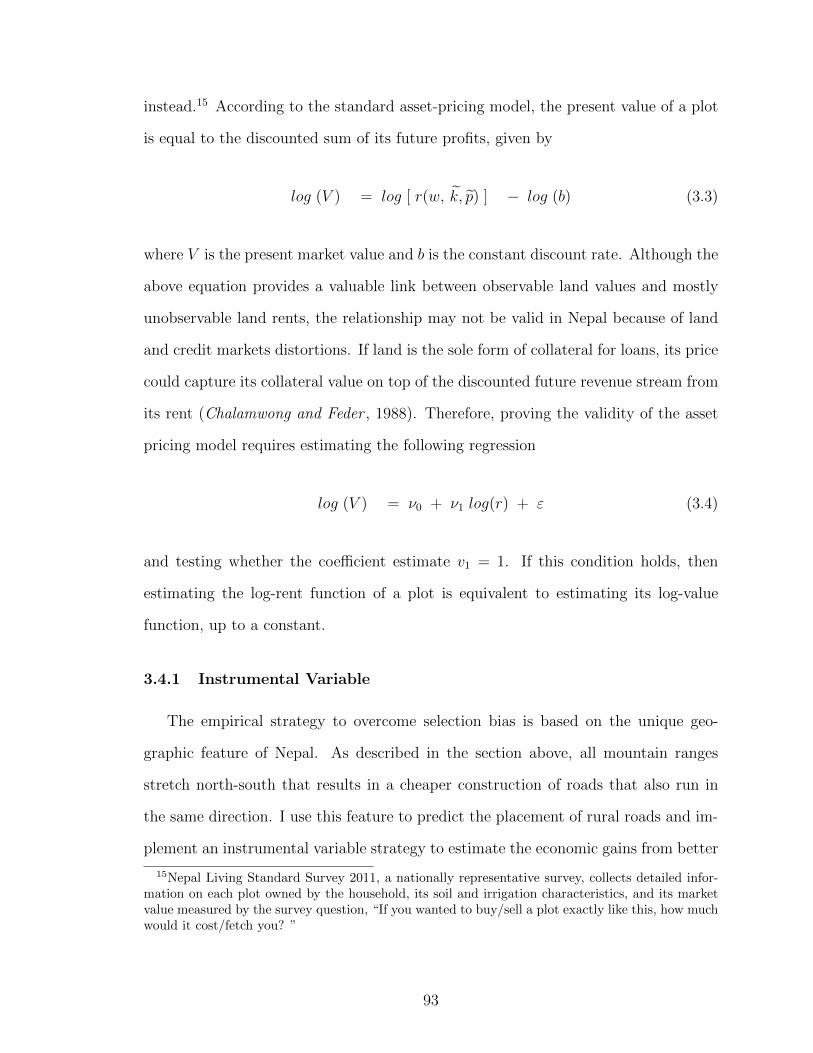
instead.15 According to the standard asset-pricing model, the present value of a plot

is equal to the discounted sum of its future profits, given by

log (V ) = log [ r(w, ek, ep) ] � log (b) (3.3)

where V is the present market value and b is the constant discount rate. Although the

above equation provides a valuable link between observable land values and mostly

unobservable land rents, the relationship may not be valid in Nepal because of land

and credit markets distortions. If land is the sole form of collateral for loans, its price

could capture its collateral value on top of the discounted future revenue stream from

its rent (Chalamwong and Feder , 1988). Therefore, proving the validity of the asset

pricing model requires estimating the following regression

log (V ) = ⌫0

+ ⌫1

log(r) + " (3.4)

and testing whether the coe�cient estimate v1

= 1. If this condition holds, then

estimating the log-rent function of a plot is equivalent to estimating its log-value

function, up to a constant.

3.4.1 Instrumental Variable

The empirical strategy to overcome selection bias is based on the unique geo-

graphic feature of Nepal. As described in the section above, all mountain ranges

stretch north-south that results in a cheaper construction of roads that also run in

the same direction. I use this feature to predict the placement of rural roads and im-

plement an instrumental variable strategy to estimate the economic gains from better

15Nepal Living Standard Survey 2011, a nationally representative survey, collects detailed infor-mation on each plot owned by the household, its soil and irrigation characteristics, and its marketvalue measured by the survey question, “If you wanted to buy/sell a plot exactly like this, how muchwould it cost/fetch you? ”

93

road accessibility for agrarian households living in the hills.

I take district headquarters that lie north of EWH and connect them using a

simple algorithm. First, I divide the country into 10 north-south blocks based on equal

longitudinal spacing. The five pairs of these adjoining blocks coincide well with the 5

development regions of Nepal,16 with each block embodying 6 district headquarters on

average. Within each block, I draw a straight line from each district headquarter to

the nearest other district headquarter. Some district headquarters could be connected

to multiple district headquarters because the nearest-headquarter pairs are not always

symmetric.17 Furthermore, restricting the connections to a north-south block ensures

that the district headquarters are connected in a north-south direction rather than

an east-west direction, which is an important feature of the instrumental variable

strategy. Lastly, I connect the district headquarter within each block that is closest

to EWH with EWH via a shortest straight line. The following algorithm results in 10

separate north-south linkages connecting the district headquarters to EWH. Figure

3.3 illustrates the 10 geographic blocks, the straight lines connecting the district

headquarters, and EWH; whereas, figure 3.4 shows the five development regions.

While 10 north-south blocks are based on the actual administrative division of Nepal,

figure 3.5 shows the outcome of a similar exercise, but using 12 geographic blocks

instead of 10 for alternate north-south linkages.

The straight line serves a proxy for NS road in the hill region. Whether the line

drawn this way coincides well with actual road network can be tested, by estimat-

ing the correlation between the distance to the line and distance to road using the

16Nepal is divided into 5 development regions: Eastern, Central, Western, Mid-Western, andFar-Western regions, starting from east to west. Figure 3.4 maps these 5 development regions.

17Suppose there are three district headquarters A, B, and C. If A is the nearest district headquarterto B and vice versa, whereas the nearest district headquarter to C is also A, then district headquarterA will be connected to both district headquarters B and C by using the above algorithm.

94

following regression framework:

log (Tid

) = ↵ + ⌘d

+ � log (Did

) + " (3.5)

where Tid

is the distance to the nearest road for rural household i living in district d,

Did

is the distance to the nearest line, and ⌘d

is district fixed e↵ects. More importantly,

Did

is influenced by two factors– administrative need to connect district headquarters

and the geographic feature that favors north-south linkages. Both of them are likely

to be independent of the socio-economic conditions of communities in the hinterlands,

providing a plausibly exogenous variation in access to infrastructure for households

in these regions.

The use of log(Did

) variable as an instrument to estimate the e↵ect of road on

farm profits requires satisfying the exclusion restriction. One potential concern in

this strategy is that Did

could be picking household’s proximity to the district head-

quarter itself, which in turn, directly a↵ects farm profits and market land values.

To address this, I control for the distance to the nearest district headquarter as well

as the distance to EWH. Banerjee et al. (2009) point out that the distance to the

straight line joining two cities in China violates the exclusion restriction because it

also coincides with the historical trade routes between those cities. In contrast, the

historical routes connecting any two cities in Nepal are equally likely to stretch east-

west as well as north-south,18 while the line is restricted to a north-south direction.

Nevertheless I control for the distance to the nearest foot trails, which constitute the

main channel through which all trades were carried out between two cities before the

construction of highways as pointed out by Stiller (1976). Finally, Did

could also be

correlated with the physical attributes of the agricultural land that directly a↵ect its

productivity and profits, I control for geographical characteristics such as distance to

river, elevation, and land gradient as well as productivity variables such as suitability

18See figure 3.2 for the mapping of historical trade routes across the country.

95

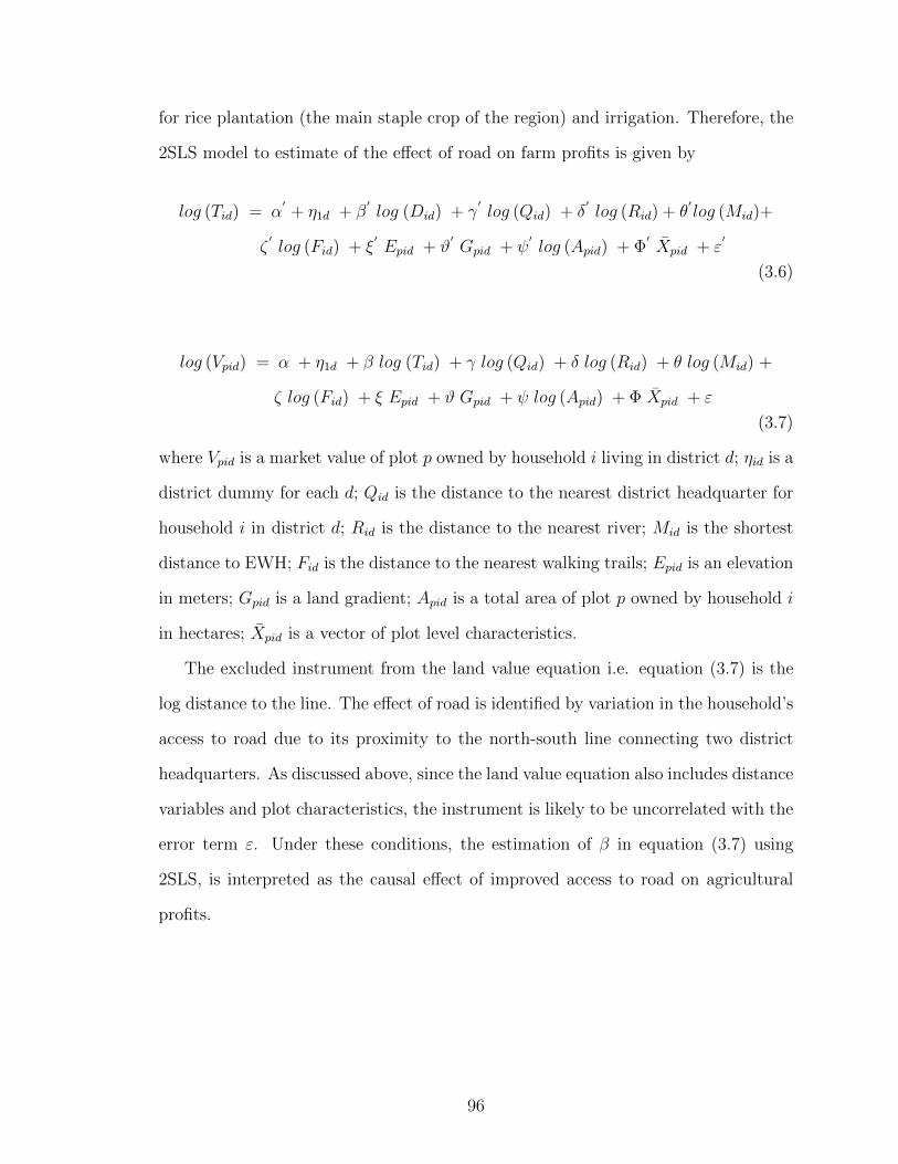
for rice plantation (the main staple crop of the region) and irrigation. Therefore, the

2SLS model to estimate of the e↵ect of road on farm profits is given by

log (Tid

) = ↵0+ ⌘

1d

+ �0log (D

id

) + �0log (Q

id

) + �0log (R

id

) + ✓0log (M

id

)+

⇣0log (F

id

) + ⇠0E

pid

+ #0G

pid

+ 0log (A

pid

) + �0X

pid

+ "0

(3.6)

log (Vpid

) = ↵ + ⌘1d

+ � log (Tid

) + � log (Qid

) + � log (Rid

) + ✓ log (Mid

) +

⇣ log (Fid

) + ⇠ Epid

+ # Gpid

+ log (Apid

) + � Xpid

+ "

(3.7)

where Vpid

is a market value of plot p owned by household i living in district d; ⌘id

is a

district dummy for each d; Qid

is the distance to the nearest district headquarter for

household i in district d; Rid

is the distance to the nearest river; Mid

is the shortest

distance to EWH; Fid

is the distance to the nearest walking trails; Epid

is an elevation

in meters; Gpid

is a land gradient; Apid

is a total area of plot p owned by household i

in hectares; Xpid

is a vector of plot level characteristics.

The excluded instrument from the land value equation i.e. equation (3.7) is the

log distance to the line. The e↵ect of road is identified by variation in the household’s

access to road due to its proximity to the north-south line connecting two district

headquarters. As discussed above, since the land value equation also includes distance

variables and plot characteristics, the instrument is likely to be uncorrelated with the

error term ". Under these conditions, the estimation of � in equation (3.7) using

2SLS, is interpreted as the causal e↵ect of improved access to road on agricultural

profits.

96

3.5 Data

The data for this study come from two major sources. The household information

on agriculture and access to infrastructure is obtained from the 2011 Nepal Living

Standards Survey (NLSS). It is a nationwide survey collected by the Central Bureau

of Statistics with a stratified random sample of 5988 households, out of which 2058

households reside in the rural hill region with farmland. The Survey includes detailed

agriculture module with information on all individual plots owned or leased by the

household, along with its area, quality, market value, irrigation, and the net rent

received by the household if the plot was leased out. Additionally, it collects infor-

mation on household’s access to various facilities, including the nearest paved road,

in terms of travel time. Travel time measures are more useful than actual distance

calculated using satellite telemetry because of mountainous terrain.

A unique feature of the 2011 NLSS is that it provides GIS information on the

location of its households. I use this GIS data to merge the Mountain Environment

and Natural Resources’ Information System (MENRIS) data for the NLSS sample

households. The MENRIS geospatial data is collected by the International Centre for

Integrated Mountain Development, ICIMOD, and has information on elevation, foot

trails, and river paths for the Hindu Kush Himalaya region including Nepal. I use

this to construct all the distance variables including the instrumental variable, and

terrain characteristics such as land gradient.

Table 3.1 provides summary statistics for rural households residing in the hills

that own a farmland along with their plot characteristics. An average landholdings

of a household is only 0.62 ha, with an average plot size of 0.19 ha. 30 percent of the

plots are categorized as being suitable for rice cultivation; whereas, almost 70 percent

of all plots do not have access to irrigation in any agriculture season.

97

3.6 Results

The relationship between rent and market value of a plot, as described by the asset-

pricing model, can be established by estimating equation (3.4). Table 3.2 presents the

estimate of coe�cient ⌘1

in equation (3.4), by using 321 plots that were either rented

out in both agricultural seasons or in the wet season. These plots were rented mainly

through sharecropping and account for about 5 % of the total plots owned. Their net

rents are calculated by summing the rents across both seasons and including the value

of in-kind payments, while the costs of inputs provided by the tenants are deducted.

The mean rent to value ratio ( r

V

) is 0.055, which can be interpreted as an estimate

of the discount rate b.19

The OLS estimate of ⌘1

in column 1 assumes that the log rent is uncorrelated with

the error term. Although the estimate is less that one, attenuation bias because of

random measurement error in rents could bias the estimate towards zero, as pointed

out by Jacoby (2000). Therefore, the specifications in columns 2 and 3 instrument

rents with plot area and column 3 additionally includes district fixed e↵ects. The

estimates, 1.12 and 1.08 respectively, are accurate and not statistically di↵erent from

unity even at the 10 % level, and therefore the validity of the asset pricing model

cannot be rejected.

Table 3.3 estimates of the impact of transportation infrastructure on the economic

gains from agriculture using a log-linear specification described by equation (3.7).

Because farmland behaves like an asset as proven by the results from table 3.2, higher

farm profits because of lower transportation costs should be capitalized in farmland

values. Therefore, the total economic benefits of having better road accessibility

for agrarian households can be calculated by estimating �, the coe�cient of the log

travel time to road in equation (3.7), where the dependent variable is the log value

19Jacoby (2000) also finds the rent to value ratio among rented lands in Nepal using 1996 NLSSto be 0.055.

98

of farmlands. Only controlling for the size of farmland, the OLS estimate of � in

column 1 is statistically significant at the 1 percent level and its value of -0.19 implies

that that an increase in the travel time to the nearest road by 10 percent decreases

the value of the farmland by 1.9 percent. However, profitable plots may encourage

larger road investments or rural roads may be more abundant in relatively more

productive regions. The inclusion of plot characteristics in columns 2 and 3, and

district fixed e↵ects in column 3, ameliorates the endogeneity problem as long as the

location of roads are determined by observed plot characteristics or by unobserved

characteristics of the district and not by unobserved characteristics of the specific

plots within the district. While the estimate in column 3 implies a strong positive

e↵ect of road on farm value, nevertheless, unobserved socio-economic and political

factors may influence road allocation within the district, which could bias the above

OLS estimates in either direction and necessitate the use of an instrumental variable

strategy to overcome the potential endogeneity bias.

Table 3.4 estimates the correlation between the travel time to the nearest road

and the distance to the nearest line by using equation (3.5). The sample is restricted

to 2058 households living in the rural hills, for which this strategy is most relevant.

Panel A presents estimates that use the line constructed based on the algorithm which

divides the region into 10 blocks; whereas, the estimates using the line constructed

with 12 blocks are shown in Panel B. All the estimates are positive and significant

at the 1 percent level, even after controlling for district fixed e↵ects in column 2 and

additionally for the distance to the nearest district HQ and the distance to EWH in

column 3.

This strong correlation suggests the possibility of using this variable as an instru-

ment in a 2SLS model described by equations (3.6) and (3.7), to estimate the e↵ect

of better access to road on land value. The threat to the validity of such a model

arises from the potential correlation of the instrumental variable with (1) proximity

99

to district headquarter, (2) closeness to the historical trade corridors, and (3) physical

characteristics of the plot. However, NLSS and MENRIS datasets have a wide set of

household and plot level information that can be used to construct these variables,

which are then included in equations (3.6) and (3.7). The measures of plot charac-

teristics include the distance to river, land gradient, elevation, a dummy indicating

whether the plot is suitable for rice cultivation, dummies indicating year round or

seasonal irrigation, and dummies indicating types of irrigation. The distance to foot

trails picks up unobserved characteristics that are correlated with the proximity to

historical trading routes; whereas the distance to the nearest district headquarter and

the distance to EWH variables control for the proximity to district headquarter and

EWH respectively.

Tables 3.5 and 3.6 estimate the reduced form e↵ect of the distance to the line

constructed by using 10 and 12 blocks algorithms, respectively. The specification in

column 1 in both tables only includes controls for district fixed e↵ects, farm size, and

the proximity to the nearest district headquarter and EWH. According to table 3.5

column 1, an increase in the distance to the line by 10 percent decreases the value of

land by 0.34 percent. As discussed above, the distance to the line could be correlated

with proximity to the historical trade corridors and physical characteristics of the

land, both of which directly a↵ect farmland value. To address this, I control for the

shortest distance to the walking trails in columns 2 and 3 and observed plot charac-

teristics in column 3. While many of these control variables have strong explanatory

power and sensible signs, the coe�cient estimates of the distance to the line do not

change considerably in magnitude from previous estimates in column 1 and are statis-

tically significant at the 1 percent level. The results show that plots suitable for rice

and plots with year round as well as seasonal irrigation are more valuable. Likewise,

an increase in land gradient negatively a↵ects the value of the land; whereas, plots

that are closer to the district headquarter or to the foot trails have greater value.

100

The coe�cient estimates on the distance to the line in table 3.5 column 2 and 3

equal -0.039 and -0.042 respectively, both of which are within a standard error of the

estimate of -0.034 from column 1. Therefore, it seems unlikely that the instrumental

variable– distance to the line– is correlated with unobserved characteristics associated

with historical proximity to trade routes and with additional land quality variables

that are not captured in the present data set, thereby bolstering the validity of the

given instrument.

Tables 3.7 and 3.8 column 3 present IV estimates of road accessibility by using

distance to the line as an instrument for the household’s travel time to the nearest

road. The estimates of the coe�cient � from the 2SLS model are -0.234 and -0.263

for the two algorithms and they are statistically significant at the 5 percent level.

The results suggest that an increase in the travel time to the nearest road by one

percent decreases the farmland value by about 0.25 percent. Table 3.9 shows the

results for the first stage of the 2SLS model by estimating coe�cient �0in equation

(3.6), which suggest that an increase in the distance to the line by one percent raises

the household’s travel time to the nearest road by 0.17 percent. The F-statistics on

the excluded variable from both algorithms in the first stage are large, 24.58 and

20.53, which indicate that the IV estimates are unlikely to be biased due to weak

instrument. Moreover, the IV estimates are robust to di↵erent parameters of the

algorithm used to construct the instrument, suggesting that an improvement in rural

road infrastructure has a positive impact on households’ economic gains from their

agricultural activities.

3.7 Conclusion

Transportation infrastructure plays a crucial role in rural development. It im-

proves agricultural productivity by reducing transaction costs (Jacoby , 2000) and

promotes e�cient labor allocation by stimulating commercialization of agriculture

101

(Gollin and Rogerson, 2010). Since many poor reside in remote locations, it provides

a direct means of reaching them, thereby facilitating e↵ective delivery of poverty

programs and basic services in health, nutrition, and education. However, evaluating

transportation projects poses a considerable challenge because roads are not randomly

placed nor it is feasible to randomize by design.

I identify a unique geographic feature of mountains in rural Nepal that allows

for a plausibly exogenous variation in the placement of rural roads. The empirical

strategy is based on the fact that two important determinants of road construction,

administrative need to connect district headquarters and the geographic feature that

favors north-south linkages, are likely to be independent of the socio-economic charac-

teristics of households living in the hinterlands. Using the distance to the north-south

line that connect two district headquarters as an instrument for road accessibility, I

find that reduction in travel time to the nearest road increases farm profits, implying

a significant economic gains to rural agricultural households.

Although it establishes a causal link between economic benefits and infrastruc-

ture investments, the distributional consequences of such projects are unclear. While

remote households have most to gain from improved access, the agricultural profits

from farmland are confined to landowners who are usually not among the very poor.

Moreover, the mechanisms through which farm profits rise are also not identified.

The most likely candidates include a greater use of modern inputs such as chemical

fertilizers and improved seeds, an easier dissemination of new farm technologies, and

an improved access to urban centers with large demand for agricultural output. These

important channels could be identified by employing a similar empirical strategy in

the future. Moreover, the benefits from road construction are not only limited to

farm profits. Gollin and Rogerson (2010) find increase in non-agricultural employ-

ment and greater urbanization due to better road network. By promoting factor

mobility and improving access to schools, road construction could also raise expected

102

returns to education, prompting households to invest more in human capital. The

empirical strategy could easily be extended to evaluate the e↵ect of road on a wider

set of economic outcomes of interest including household’s education, health, nutri-

tion, and migration decisions, which are important determinants of its welfare and

its community’s long term economic development.

103

Figure 3.1: The Physical Map of Nepal

"/Users/sleshshrestha/Dropbox/University of Michigan/Research/Chapter 3-Roads/Figures/elevation nepal"-eps-converted-to.pdf

Notes: The figure illustrates the ruggedness of the terrain. While the thin southernstretch of the country is flat and uniform, the land surface north of the Terrai plainis characterized by sharp changes in elevation as illustrated by the compactness ofcontour lines.

104

Figure 3.2: Historical Trade Routes and Walking Trails

"/Users/sleshshrestha/Dropbox/University of Michigan/Research/Chapter 3-Roads/Figures/Nepal roads, district border, district HQ"-eps-converted-to.pdf

Notes: The figure plots the walking trails that span the country. The district head-quarters are illustrated by dotted points on the map. The foot trails stretch in anorth-south as well as an east-west directions.

105

Figure 3.3: Lines Constructed by Connecting District Headquarters (Using 10 Blocks

Algorithm)

"/Users/sleshshrestha/Dropbox/University of Michigan/Research/Chapter 3-Roads/Figures/GRID10"-eps-converted-to.pdf

106

Figure 3.4: Five Development Regions of Nepal

"/Users/sleshshrestha/Dropbox/University of Michigan/Research/Chapter 3-Roads/Figures/development region nepal"-eps-converted-to.pdf

107

Figure 3.5: Lines Constructed by Connecting District Headquarters (Using 12 Blocks

Algorithm)

"/Users/sleshshrestha/Dropbox/University of Michigan/Research/Chapter 3-Roads/Figures/GRID12"-eps-converted-to.pdf

108

Figure 3.6: Flow of Rivers and Streams

"/Users/sleshshrestha/Dropbox/University of Michigan/Research/Chapter 3-Roads/Figures/Nepal rivers, district borders, district HQ"-eps-converted-to.pdf

109

Figure 3.7: Elevation

"/Users/sleshshrestha/Dropbox/University of Michigan/Research/Chapter 3-Roads/Figures/Nepal elevation, district borders, district HQ"-eps-converted-to.pdf

Notes: Blue indicate low elevation land and red indicates high elevation. The eleva-tions changes drastically going from north to south, while the elevation remains fairlyconstant going from east to west.

110

Table 3.1: Descriptive Statistics

Mean Std. Dev

Panel A: HH Characteristics

Number of Households 2058 -Land Area (Ha) 0.62 0.62Number of Plots 3.30 2.19Household Size 4.76 2.10Travel Time to Paved Road (Hrs) 7.42 13.48

Panel B: Plot Characteristics

Number of Plots 6785 -Plot Size (Ha.) 0.19 0.25Plot Value (Million Rs. per Ha.) 3.04 17.47% Suitable for Rice 30.79 46.17% with Year Round Irrigation 14.62 35.33% with Seasonal Irrigation 16.34 36.98% with Tubewell 0.87 9.29% with Canal 25.78 43.74% with Pond 0.25 4.99% with Mixed 0.29 5.42Elevation (Meters) 1215.45 457.63Land Gradient (Degrees) 24.29 11.35

Panel C: Distance Variables (in Km)

Distance to the Line (10 Blocks) 11.51 9.41Distance to the Line (12 Blocks) 11.88 9.06Distance to District Headquarters 15.95 8.82Distance to EWH 51.75 21.18Distance to River 0.84 0.59Distance to Foot Trails 1.25 1.26

Notes: The household and plot samples are restricted to rural hill region. The householdand plot level data in Panels A and B (except elevation and land gradient) is obtained from2011 Nepal Living Standard Survey. The rest of the data including distance variables arecalculated using MENRIS data.

111

Table 3.2: Relationship Between Plot Values and Rents

(1) (2) (3)OLS IV⌧ IV⌧

Log Rent (v1

) 0.69** 1.12** 1.08**(0.0560) (0.1122) (0.1152)

Ho: v1

= 1 (p-value) 0.000 0.255 0.439

District Fixed E↵ect No No YesNumber of Plots 327 327 327

Notes: This table reports the coe�cient of the log of rent from equation (3.4), where thedependent variable is the log of plot market value. If the asset-pricing model is valid andmarket value of the plot is equal to the discounted future rent stream, then this coe�cientv1

= 1. The table also presents the p-value of this test.⌧ Log of plot area is the excluded instrument.* indicates significance at the 5 percent level** indicates significance at the 1 percent level

112

Table 3.3: E↵ect of Road on Land Value (OLS)

(1) (2) (3)

Log Travel Time to Road -0.190*** -0.173*** -0.146***(0.0058) (0.0056) (0.0060)

Log Plot Area 0.708*** 0.677*** 0.670***(0.0156) (0.0150) (0.0137)

Irrigation:Year-Round 0.582*** 0.663***

(0.0978) (0.0859)Seasonal 0.088 0.293***

(0.0876) (0.0767)Mode of Irrigation:

Tubewell 0.824* 0.240(0.1788) (0.1568)

Canal -0.037 -0.006(0.0837) (0.0730)

Pond 0.452 0.145(0.3054) (0.2640)

Mixed 0.540* 0.401(0.2827) (0.2448)

Plot Quality:Suitable for Rice 0.458*** 0.211***

(0.0520) (0.0462)

District Fixed E↵ect No No YesR Squared 0.301 0.361 0.530Number of Plots 6750 6750 6750

*significance at the 10 percent level ** significance at the 5 percent level *** significance at the 1 percent level

113

Table 3.4: Relation Between Travel Time to Road and Distance to the Line

(1) (2) (3)

Panel A: 10 BlocksLog Distance to the Line 0.623*** 0.603*** 0.205***

(0.0576) (0.0554) (0.0682)Log Distance to District Headquarter 1.174***

(0.117)Log Distance to EWH 0.724***

(0.184)

R Squared 0.055 0.431 0.463

Panel B: 12 BlocksLog Distance to the Line 0.592*** 0.640*** 0.237***

(0.0601) (0.0574) (0.0719)Log Distance to District Headquarter 1.145***

(0.1190)Log Distance to EWH 0.754***

(0.1840)

R Squared 0.046 0.433 0.463

District Fixed E↵ect No Yes YesNumber of HHs 2025 2025 2025

Notes:* indicates significance at the 5 percent level** indicates significance at the 1 percent level

114

Table 3.5: E↵ect of Road on Land Value Using 10 Blocks (Reduced Form)

(1) (2) (3)

Log Distance to the Line -0.034* -0.039** -0.042**(0.0196) (0.0196) (0.0187)

Log Plot Area 0.696*** 0.696*** 0.676***(0.0147) (0.0147) (0.0141)

Irrigation:Year-Round 0.622***

(0.0874)Seasonal 0.258***

(0.0783)Mode of Irrigation:

Tubewell 0.287*(0.159)

Canal 0.066(0.0744)

Pond 0.239(0.270)

Mixed 0.552**(0.269)

Plot Quality:Suitable for Rice 0.200***

(0.0474)Land Gradient -0.169***

(0.0168)Log Distance to River 0.007

(0.0138)Log Distance to District Headquarter -0.338*** -0.335*** -0.255***

(0.0335) (0.0335) (0.0327)Log Distance to Foot Trails -0.044*** -0.041***

(0.0116) (0.0111)Log Distance to EWH 0.203*** 0.191*** 0.298***

(0.0559) (0.0559) (0.0601)Elevation -0.000***

(0.0000)

District Fixed E↵ect Yes Yes YesR Squared 0.457 0.458 0.511Number of Plots 6745 6745 6745


115

Table 3.6: E↵ect of Road on Land Value Using 12 Blocks (Reduced Form)

(1) (2) (3)

Log Distance to the Line -0.0502** -0.0489** -0.0449**(0.0204) (0.0204) (0.0195)

Log Plot Area 0.698*** 0.697*** 0.677***(0.0147) (0.0147) (0.0141)

Irrigation:Year-Round 0.624***

(0.0873)Seasonal 0.263***

(0.0783)Mode of Irrigation:

Tubewell 0.281*(0.1590)

Canal 0.065(0.0744)

Pond 0.244(0.2700)

Mixed 0.558**(0.2690)

Plot Quality:Suitable for Rice 0.197***

(0.0474)Land Gradient -0.167***

(0.0168)Log Distance to River 0.008

(0.0138)Log Distance to District Headquarter -0.322*** -0.325*** -0.251***

(0.0340) (0.0340) (0.0333)Log Distance to Foot Trails -0.042*** -0.039***

(0.0116) (0.0111)Log Distance to EWH 0.194*** 0.183*** 0.295***

(0.0561) (0.0561) (0.0601)Elevation -0.000***

(0.0000)

District Fixed E↵ect Yes Yes YesR Squared 0.457 0.458 0.511Number of Plots 6745 6745 6745


116

Table 3.7: E↵ect of Road on Land Value Using 10 Blocks (IV)

(1) (2) (3)OLS Reduced Form IV⌧

Log Travel Time to Road -0.130*** - -0.234**(0.00627) (0.1050)

Log Distance to the Line - -0.042** -(0.0187)

Log Plot Area 0.686*** 0.676*** 0.692***(0.0137) (0.0141) (0.0152)

Irrigation:Year-Round 0.684*** 0.622*** 0.724***

(0.0852) (0.0874) (0.0959)Seasonal 0.305*** 0.258*** 0.334***

(0.0761) (0.0783) (0.0827)Mode of Irrigation:

Tubewell 0.212 0.287* 0.169(0.1560) (0.1590) (0.1640)

Canal -0.012 0.066 -0.064(0.0725) (0.0744) (0.0903)

Pond 0.086 0.239 -0.028(0.2620) (0.2700) (0.2900)

Mixed 0.459* 0.552** 0.380(0.2610) (0.2690) (0.2770)

Plot Quality:Suitable for Rice 0.176*** 0.200*** 0.159***

(0.0461) (0.0474) (0.0498)Land Gradient -0.126*** -0.169*** -0.093**

(0.0164) (0.0168) (0.0374)Log Distance to River 0.019 0.007 0.028*

(0.0134) (0.0138) (0.0165)Log Distance to District Headquarter -0.178*** -0.255*** -0.084

(0.0264) (0.0327) (0.0991)Log Distance to Foot Trails -0.032*** -0.041*** -0.024*

(0.0108) (0.0111) (0.0135)Log Distance to EWH 0.361*** 0.298*** 0.395***

(0.0590) (0.0601) (0.0689)Elevation -0.000 -0.000*** -0.005

(0.0001) (0.0000) (0.0001)

F-Statistics on Instrument 24.58Probability>F 0.000

⌧ Log Distance to the Line is the excluded instrument. All specifications include district fixed e↵ect.


117

Table 3.8: E↵ect of Road on Land Value Using 12 Blocks (IV)

(1) (2) (3)OLS Reduced Form IV⌧

Log Travel Time to Road -0.130*** - -0.263**(0.00627) (0.1160)

Log Distance to the Line - -0.045** -(0.0195)

Log Plot Area 0.686*** 0.677*** 0.694***(0.0137) (0.0141) (0.0156)

Irrigation:Year-Round 0.684*** 0.624*** 0.736***

(0.0852) (0.0873) (0.0989)Seasonal 0.305*** 0.263*** 0.342***

(0.0761) (0.0783) (0.0848)Mode of Irrigation:

Tubewell 0.212 0.281* 0.157(0.1560) (0.1590) (0.1670)

Canal -0.012 0.0649 -0.0779(0.0725) (0.0744) (0.0944)

Pond 0.086 0.244 -0.0591(0.2620) (0.2700) (0.2980)

Mixed 0.459* 0.558** 0.358(0.2610) (0.2690) (0.2830)

Plot Quality:Suitable for Rice 0.176*** 0.197*** 0.154***

(0.0461) (0.0474) (0.0510)Land Gradient -0.126*** -0.167*** -0.084**

(0.0164) (0.0168) (0.0408)Log Distance to River 0.019 0.00842 0.031*

(0.0134) (0.0138) (0.0173)Log Distance to District Headquarter -0.178*** -0.251*** -0.058

(0.0264) (0.0333) (0.1090)Log Distance to Foot Trails -0.032*** -0.039*** -0.022

(0.0108) (0.0111) (0.0141)Log Distance to EWH 0.361*** 0.295*** 0.404***

(0.0590) (0.0601) (0.0713)Elevation -0.000 -0.000*** 0.000

(0.0001) (0.0000) (0.0000)F-Statistics on Instrument 20.53Probability>F 0.000

⌧ Log Distance to the Line is the excluded instrument. All specifications include district fixed e↵ects.


118

Table 3.9: Travel Time to Road and Distance to the Line (First Stage)

(1) (2)10 Blocks 12 Blocks

Log Distance to the Line 0.176*** 0.167***(0.0355) (0.0370)

Log Plot Area 0.061** 0.055**(0.0267) (0.0267)

Irrigation:Year-Round 0.432*** 0.418**

(0.1660) (0.1660)Seasonal 0.311** 0.291**

(0.1490) (0.1480)Mode of Irrigation:

Tubewell -0.483 -0.451(0.3040) (0.3030)

Canal -0.532*** -0.523***(0.1410) (0.1410)

Pond -1.129** -1.142**(0.5100) (0.5100)

Mixed -0.730 -0.752(0.5100) (0.5100)

Plot Quality:Suitable for Rice -0.162* -0.153*

(0.0898) (0.0899)Land Gradient 0.323*** 0.314***

(0.0318) (0.0318)Log Distance to River 0.090*** 0.086***

(0.0261) (0.0261)Log Distance to District HQ 0.730*** 0.736***

(0.0618) (0.0631)Log Distance to Foot Trails 0.081*** 0.072***

(0.0211) (0.0211)Log Distance to EWH 0.338*** 0.347***

(0.1150) (0.1150)Elevation 0.001*** 0.001***

(0.0000) (0.0000)

District Fixed E↵ect Yes YesR Squared 0.445 0.445Number of Plots 6710 6710

* indicates significance at the 10 percent level ** indicates significance at the 5 percent level*** indicates significance at the 1 percent level

119

BIBLIOGRAPHY

120

BIBLIOGRAPHY

Abadie, A., and J. Gardeazabal (2003), The economic costs of conflict: A case studyfor the basque country, The American Economic Review, 93 (1), 113–132.

Angelucci, M., G. DeGiorgi, M. A. Rangel, and I. Rasul (2009), Family networks andschool enrollment: Evidence from a randomized social experiment, NBER WorkingPaper.

Angrist, J., and V. Lavy (1999), Using maimonides’ rule to estimate the e↵ect of classsize on scholastic achievement, Quarterly Journal of Economics, 114 (2), 533–575.

Angrist, J. D., and G. W. Imbens (1995), Two-stage least squares estimation ofaverage causal e↵ects in models with variable treatment intensity, Journal of theAmerican Statistical Association, 90 (430), 431–442.

Arnott, R. J., and J. E. Stiglitz (1981), Aggregate land rents and aggregate transportcosts, The Economic Journal, 91 (362), 331–347.

Atack, J., F. Bateman, M. Haines, and R. Margo (2009), Did railroads induce or followeconomic growth? urbanization and population growth in the american midwest,1850-60, NBER Working Paper No. 14640.

Banerjee, A., E. Duflo, and N. Qian (2009), On the road: Access to transportationinfrastructure and economic growth in china.

Banskota, P. (1994), The Gurkha Connection: A History of the Gurkha Recruitmentin the British Indian Army, Nirala Publications.

Becker, G. (1965), A theory of the allocation of time, Economic Journal, 75, 493–517.

Becker, G. (1981), A Treaties on the Family, Harvard University Press.

Behrman, J. R., R. Pollak, and P. Taubman (1982), Parental preferences and provisionfor progeny, The Journal of Political Economy, 90 (1), 52–73.

Beine, M., F. Docquier, and H. Rapoport (2006), Brain drain and human capitalformation in developing countries : Winners and losers, university catholique deLouvain, Departement des Sciences Economiques.

Bertrand, M., E. Duflo, and S. Mullainathan (2004), How much should we trustdi↵erences-in-di↵erences estimates?, Quarterly Journal of Economics, 119 (1), 249–275.

121

Bhagwati, J., and K. Hamada (1974), The brain drain, international integration ofmakets for professionals and unemployment, Journal of Development Economics,1, 19–42.

Bommier, A., and S. Lambert (2000), Education demand and age at school enrollmentin tanzania, The Journal of Human Resources, 35 (1), 177–203.

Burgess, R., and R. Jedwab (2010), Our turn to eat: The political economy of roadsin kenya.

Caplan, L. (1995), Warrior Gentlemen: Gurkhas in the Western Imagination,Berghahn Books.

Chalamwong, Y., and G. Feder (1988), The impact of landownership security: Theoryand evidence from thailand, World Bank Economic Review, 2, 187–204.

Chand, S., and M. A. Clemens (2008), Skilled emigration and skill creation: A quasi-experiment.

Docquier, F., O. Lohest, and A. Marfouk (2007), Brain drain in developing countries,World Bank Economic Review, 21 (2), 193–218.

Donaldson, D. (2010), Railroads and the raj: The economic impact of transportationinfrastructure.

Duflo, E., and R. Hanna (2005), Monitoring works: Getting teachers to come toschool, NBER Working Paper, 11880.

Fafchamps, M., and R. V. Hill (2005), Selling at the farm-gate or travelling to market,American Journal of Agricultural Economics, 87 (3), 717–734.

Foster, A. D., and M. R. Rosenzweig (1996), Technical change and human-capitalreturns and investments: Evidence from the green revolution, The American Eco-nomic Review, 86 (4), 931–953.

Gollin, D., and R. Rogerson (2010), Agriculture, roads, and economic developmentin uganda, NBER Working Paper No. 15863.

Gronau, R. (1977), Leisure, home production and work: The theory of the allocationof time revisted, Journal of Political Economy, 85 (6), 1099–1123.

Haque, N. U., and S.-J. Kim (1995), Human capital flight: Impact of migration onincome and growth, IMF Sta↵ Papers, 42 (3), 577–607.

Hitchcock, J. T. (1966), The Magars of Banyan Hill, Holt, Rinehart, and Winston.

Jacoby, H. G. (2000), Access to markets and the benefits of rural roads, The EconomicJournal, 110 (465), 713–737.

122

Jacoby, H. G., and B. Minten (2008), On measuring the benefits of lower transportcosts, World Bank Policy Research Working Paper 4484.

Jensen, R. (2010), The (perceived) returns to education and the demand for schooling,The Quarterly Journal of Economics, 125 (2), 515–548.

Kochar, A. (2004), Urban influences on rural schooling in india, Journal of Develop-ment Economics, 74, 113–136.

Kremer, M., E. Miguel, and R. Thornton (2009), Incentives to learn, Review of Eco-nomics and Statistics, 91 (3), 437–456.

Lee, J. (2008), Sibling size and investment in children’s education: An asian instru-ment, Journal of Population Economics, 21 (4), 855–875.

Manski, C. F. (1993), Identification of endogenous social e↵ects: The reflection prob-lem, The Review of Economic Studies, 60 (3), 531–542.

Mansuri, G., S. A. Shrestha, H. Winkler, and M. Yanez-Pagans (2012a), A plot ofmy own: Property rights and economic mobility in rural uganda.

Mansuri, G., S. A. Shrestha, H. Winkler, and M. Yanez-Pagans (2012b), Health ordeath? health shock of an income earner and economic mobility in rural pakistan.

McKenzie, D., and H. Rapoport (2006), Can migration reduce educational attain-ment? evidence from mexico, World Bank Policy Research Working Paper 3952.

Meyer, W. (2008), Nepal-roads to prosperity partnership results, Tech. rep., SDCSwiss Agency for Development and Cooperation.

Michaels, G. (2008), The e↵ect of trade on the demand for skill-evidence from theinterstate highway system, Review of Economics and Statistics, 90 (4).

Miyagiwa, K. (1991), Scale economies in education and the brain drain problem,International Economic Review, 32 (3), 743–759.

Mountford, A. (1997), Can a brain drain be good for growth in the source country?,Journal of Development Economics, 53(2), 287–303.

Newman, J. L., and P. J. Gertler (1994), Family productivity, labor supply, andwelfare in a low income country, The Journal of Human Resources, 29 (4), 989–1026.

Oyelere, R. U. (2009), Understanding low average returns to education in africa: Therole of heterogeneity across education levels and the importance of political andeconomic reforms.

Pitt, M. M., M. R. Rosenzweig, and M. N. Hassan (1990), Productivity, health, andinequality in the intrahosuehold distribution of food in low-income countries, TheAmerican Economic Review, 80 (5), 1139–1156.

123

Qian, N. (2009), Quantity-quality and the one child policy: The only-child disadvan-tage in school enrollment in rural china, NBER Working Paper.

Rathaur, K. R. S. (2001), British gurkha recruitment: A historical perspective, Voiceof History, 16(2), 19–24.

Rosenzweig, M. R., and K. I. Wolpin (1980), Testing the quanity-quality fertilitymodel: The use of twins as a natural experiment, Econometrica, 48 (1), 227–240.

Schultz, P. T. (2004a), School subsidies for the poor: Evaluating the mexican progresapoverty program, Journal of Development Economics, 74 (1), 199–250.

Schultz, T. P. (2004b), School subsidies for the poor: Evaluating the mexican progresapoverty program, Journal of Development Economics, 74 (1), 199–250.

Schultz, T. W. (1975), The value of the ability to deal with disequilibria, Journal ofEconomic Literature, 13 (3), 827–846.

Shrestha, B., and S. Jain (1977), Regional Development in Nepal, Development, NewDelhi.

Shrestha, N. R. (2001a), The Political Economy of Land, Landlessness and Migrationin Nepal, Nirala Series.

Shrestha, N. R. (2001b), The Political Economy of Land, Landlessness and Migrationin Nepal, Nirala Series.

Shrestha, S. A. (2011), E↵ects of educational returns abroad on domestic schooling:A british gurkha amry experiment.

Shrestha, S. H. (2004), Economic Goegraphic of Nepal, Educational Publishing House.

Stark, O., C. Helmenstein, and A. Prskawetz (1997), A brain gain with a brain drain,Economic Letters, 55 (2), 227–234.

Stiller, L. (1976), The Silent Cry, Sahayogi Prakashan, Kathmandu.

Strauss, J., and D. Thomas (1995), Human resources: Empirical modeling of house-hold and family decision, Handbook of Development Economics, 3, 1885–2005.

Upadhyaya, S. K. (2010), Upland poverty in nepal: The role of environment, Tech.rep., Institute for Integrated Development Studies.

124

essays on the empirical study of migration, intrahousehold trade

Documents