essd-2019-84 preprint. discussion started: 1 august 2019 ... · for example, in low resolution mode...
TRANSCRIPT

1
5
Global River Radar Altimetry Time Series (GRRATS): New River Elevation Earth Science Data Records for the Hydrologic Community Stephen Coss1,2, Michael Durand1,2, Yuchan Yi1, Yuanyuan Jia1, Qi Guo1, Stephen Tuozzolo1, C. K. Shum1,6, George H. Allen3,4, Stéphane Calmant5, Tamlin Pavelsky3
1 School of Earth Sciences, The Ohio State University, Columbus, Ohio, USA 2Byrd Polar and Climate Research Center, The Ohio State University, Columbus, Ohio, USA
3Department of Geological Sciences, The University of North Carolina at Chapel Hill, USA 4Department of Geography, Texas A&M University, College Station, TX, USA 10
5IRD/LEGOS, 16 Avenue Edouard Belin, 31400 Toulouse, France 6Institute of Geodesy and Geophysics, Chinese Academy of Sciences, Wuhan 430077, China
Correspondence to: Stephen Coss ([email protected])
Abstract. The capabilities of radar altimetry to measure inland water bodies are well established and several river altimetry 15
datasets are available. Here we produced a globally-distributed dataset, the Global River Radar Altimeter Time Series
(GRRATS), using Envisat and Ocean Surface Topography Mission (OSTM)/Jason-2 radar altimeter data spanning the time
period 2002–2016. We developed a method that runs unsupervised, without requiring parameterization at the measurement
location, dubbed virtual station (VS) level and applied it to all altimeter crossings of ocean draining rivers with widths
>900 m (>34% of global drainage area). We evaluated every VS, either quantitatively for VS where in-situ gages are 20
available, or qualitatively using a grade system. We processed nearly 1.5 million altimeter measurements from 1,478 VS.
After quality control, the final product contained 810,403 measurements distributed over 932 VS located on 39 rivers.
Available in-situ data allowed quantitative evaluation of 389 VS on 12 rivers. Median standard deviation of river elevation
error is 0.93 m, Nash-Sutcliffe efficiency is 0.75, and correlation coefficient is 0.9. GRRATS is a consistent, well-
documented dataset with a user-friendly data visualization portal, freely available for use by the global scientific community. 25
Data are available at DOI 10.5067/PSGRA-SA2V1(Durand et al., 2016).
https://doi.org/10.5194/essd-2019-84
Ope
n A
cces
s Earth System
Science
DataD
iscussio
ns
Preprint. Discussion started: 1 August 2019c© Author(s) 2019. CC BY 4.0 License.
2
1 Introduction
Despite growing demand from emerging large-scale hydrologic science and applications, global and freely available
observations of river water levels are still scarce (Hannah et al., 2011; Pavelsky et al., 2014; Shiklomanov et al., 2002).
Advances in remote sensing and computing capabilities have enabled new areas of global fluvial research that are dependent
upon river elevations, including global hydrologic quantification of carbon and nitrogen fluxes (e.g. Allen & Pavelsky, 2018; 5
Oki & Yasuoka, 2008) and characterizing flood risk for future climate scenarios (Schumann et al., 2018; Smith et al., 2015).
Evaluation of these global river elevation models requires global datasets of river elevation time series, but in situ river water
levels are scarce, as they are often not shared outside specific government agencies. Thus model evaluation and calibration
increasingly relies on remotely sensed data (Overton, 2015; Pavelsky et al., 2014; Sampson et al., 2015). Newer radar
altimeter missions like Sentinel-3 are improving the contemporary record with features like automated processing. In 10
addition, the Surface Water and Ocean Topography (SWOT; swot.jpl.nasa.gov) satellite mission, scheduled for launch in
2021, will observe global river elevations with an unprecedented global spatial resolution despite variation within its
measurement swath. Establishing robust global river elevation datasets for the pre-SWOT period is critical to prepare for the
SWOT mission and for the study of hydrology more broadly.
Satellite radar altimetry data have enabled important scientific advances in hydrology (Birkett et al., 2002; Bjerklie et al., 15
2005; Calmant et al., 2008; Jung et al., 2010, Guetirana et al., 2009, Birkinshaw et al., 2014, Frappart et al., 2015, Becker et
al., 2018, Emery et al., 2018, among many others), but spatial coverage is limited. This is for two primary reasons:
inclination or latitude coverage limits of radar altimeter orbits (orbits with better temporal resolution have worse spatial
coverage), and technical measurement challenges associated with retrieving elevation over seasonally varying rivers. Indeed,
radar altimeter orbits and elevation retrieval technology were originally designed for characterizing ocean surface 20
topography. The orbital characteristics of historic and contemporary radar altimetry missions used for hydrology tend to
follow either the 10-day TOPEX/POSIEDON/Jason-1/-2/-3 orbit with relative high temporal resolution but low spatial
coverage, or the 35-day ERS-1/-2/Envisat/SARAL-AltiKa orbits with low temporal resolution but higher spatial coverage.
Neither of these orbit paradigms capture all global rivers (Alsdorf et al., 2007).
The second fundamental cause of poor global coverage of river radar altimeter observation availability is rooted in the 25
measurement itself. There are a set of criteria, such as river width, nearby topography, and groundcover, associated with
successful water surface level retrieval, but none have been shown to be fully predictive of water level accuracy (Maillard et
al., 2015). Most of Earth’s rivers are too narrow to be accurately be measured by satellite radar altimeters: Lettenmaier et al.
(2015) suggest that rivers should be wider than 1,000 m for optimal retrieval, primarily due to the 1–2 km footprint size of
pulse-limited satellite altimeters. Radar altimeter effective footprint size is a function of the surface characteristics and pulse 30
emission mode. For example, in Low Resolution mode (LRM), which was commonly used for satellite altimeters until
~2016, footprints typically range from 1.5 to 6.0 km in diameter, depending on the land topography near rivers. Thus, all but
the widest rivers are (technically) sub-footprint features in LRM. Radar altimetry retrieval of river surface elevations thus
https://doi.org/10.5194/essd-2019-84
Ope
n A
cces
s Earth System
Science
DataD
iscussio
ns
Preprint. Discussion started: 1 August 2019c© Author(s) 2019. CC BY 4.0 License.
3
relies on the fact that rivers reflect more radar signal than does land, due to the high dielectric constant of water. Some
studies have developed methods to process radar altimetry data for far narrower rivers with LRM altimeters (e.g. ~100 m) for
a particular location (e.g. Santo da Silva, 2010., Maillard et al., 2015, Boergens et al., 2016, Biancamaria et al.,2017). Since
~2016, retrieving water levels over narrow rivers is increasingly common with the Synthetic Aperture Radar (SAR) altimetry
missions (e.g. Cryosat-2 and Sentinel-3) for which the equivalent footprint (300 m wide along flight track band) enables 5
much easier detection and processing of radar returns from rivers.
Regardless of the specifics of a particular measurement location, altimeter range data (direct sensor measurement) requires a
great deal of processing to be converted into usable surface heights. Measurements of ocean height rely on an onboard
processor known as a “tracker” to dynamically estimate the approximate range of the target (i.e. the sea surface) in order to
map received radar pulses to precise surface elevations. The onboard tracker works well for measuring ocean surface 10
elevations, but it is unsuitable for estimating continental surface elevations. It thus requires further processing steps, known
as “retracking”. Using retracked river observations, inland radar altimetry can accurately measure changing river surface
elevation (Koblinsky et al., 1993, Berry et al., 2005; Frappart et al., 2006; Alsdorf et al., 2007; Santos da Silva et al., 2010;
Papa et al., 2010; Dubey et al., 2015, Tourian et al., 2016, Verron et al., 2018). While custom retrackers have been derived
and tested in particular locations (Huang et al., 2018; Maillard et al., 2015; Sulistioadi et al., 2015) the ICE-1 retracker 15
(Wingham et al., 1986) is arguably the best compromise between being consistently reliable and available for many altimeter
missions (Biancamaria et al., 2017; Frappart et al., 2006; Santos da Silva et al., 2010). While available globally, the ICE-1
retracked data must be extracted over river targets, and carefully filtered, to make them useful to global hydrological
modeling applications.
The four currently available radar altimeter datasets for rivers represent tremendous technical achievements: 1) Hydroweb 20
(hydroweb.theia-land.fr); 2)DAHITI(dahiti.dgfi.tum.de); 3) River&LakeNRT(https://web.archive.org/web/20180721182437/
http://tethys.eaprs.cse.dmu.ac.uk/RiverLake/shared/main); and 4) HydroSat (hydrosat.gis.uni-stuttgart.de/php/index.php).
However, they are not optimized for the specific needs of global hydrologic modelers, who require global coverage, and
enhanced ease of use (accessibility and metadata). Note that River&LakeNRT is no longer online but we compare against it
for historical reasons (an archive link has been provided). Existing datasets have several characteristics that make them 25
challenging to use for global hydrologic modeling. First, they tend to include dense coverage where altimeters perform well
(e.g. over large, tropical rivers), or based on programmatic priorities of funding agencies. VS are the fundamental
organizational element for GRRATS (as well as other altimetry datasets for rivers). VS are locations where ground tracks of
exact repeat altimetry mission orbits cross rivers, enabling a time series of water elevation observations. Hydroweb has 991
river virtual stations (VS) in South America alone, for example, primarily in the Amazon basin, while most include few 30
Arctic rivers. One challenge of including Arctic rivers involves the complicating effect of river ice, which is widespread for
much of the year. Three of the four datasets (Hydroweb being the exception), cannot be downloaded in bulk, but require
repetitive clicking via web interface.
https://doi.org/10.5194/essd-2019-84
Ope
n A
cces
s Earth System
Science
DataD
iscussio
ns
Preprint. Discussion started: 1 August 2019c© Author(s) 2019. CC BY 4.0 License.

4
In this study, we determined what fraction of available altimeter data would be useful for global rivers using retracked data
available from the official distribution of the instrument data (the geophysical data records (GDR)), unsupervised methods,
and automatic data filtering processes. The result is the Global River Radar Altimetry Time Series (GRRATS), a global river
altimetry dataset comprised of an opportunistic exploitation of VS on the world’s largest rivers specifically suited for the
needs of global hydrological applications. GRRATS is an “Earth Science Data Record” (ESDR) hosted at Physical 5
Oceanography Distributed Active Archive Center (PO.DAAC) with a focus on conforming to data management and
stewardship best practices (Wilkinson et al., 2016). GRRATS currently spans 2002 – 2016, and includes global ocean-
draining rivers greater than 900 m in width: these collectively drain a total of >34% of global land area. GRRATS follows
data management best practices as outlined by Wilkinson et al. (2016), and it includes extensive metadata. In developing
GRRATS, our purpose is to create an accurate dataset, and also to create a better data product focused on ease of use. 10
2 Methods
There are four major steps in building GRRATS (Durand et al., 2016): 1) identification of potential VS on global rivers; 2)
extraction of altimeter observations from the Geophysical Data Records (GDRs); 3) filtering out noisy returns from the
altimetry; and 4) performing either quantitative of qualitative evaluation. The philosophy and overview of GRRATS
methods are reviewed here, whereas details of GRRATS production are more thoroughly described in the User Handbook 15
(ftp://podaac-ftp.jpl.nasa.gov/allData/preswot_hydrology/L2/rivers/docs/).
2.1 Identification of potential VS
We began by identifying potential VS for GDR extraction by identifying locations on global ocean-draining rivers where
altimeter orbital ground tracks cross river locations greater than 900 m in width. We chose 900m as our lower width limit as 20
previous work has shown that VS with widths >1 km present a higher probability of good performance (Birkett et al., 2002;
Frappart et al., 2006; Kuo & Kao, 2011; Papa et al., 2012). This selection of rivers is spatially varied and large enough to
provide a sensible constraint on global models. We used the intersection of the nominal altimeter ground tracks with the
Global River Widths from Landsat (GRWL) dataset to identify such locations (Allen & Pavelsky, 2018).
2.2 GDR extraction 25
We extracted altimeter observations at the VS from the GDRs; this consisted of three steps. First we spatially joined Landsat
imagery (selected from times of mean river discharge) compiled for the GRWL river centerlines dataset (Allen & Pavelsky,
2015; Allen & Pavelsky, 2018) with satellite ground tracks to define the extent of the mask used for the extraction of water
elevations. We extracted all altimeter returns with centroids falling within each polygon for each pass from Jason-2
Geophysical Data Record (GDR) version D (Dumont et al., 2009), and the Envisat GDR, Version 2.1 or later (Soussi & 30
https://doi.org/10.5194/essd-2019-84
Ope
n A
cces
s Earth System
Science
DataD
iscussio
ns
Preprint. Discussion started: 1 August 2019c© Author(s) 2019. CC BY 4.0 License.
5
Féménias, 2009), using corrections outlined in product documentation. We extracted ICE-1 retracked ranges from the GDR
(Gommenginger et al., 2011; Wingham et al., 1986). To get ellipsoidal heights, we applied the standard combination of
parameters and corrections. We then converted these ellipsoidal heights to an orthometric height above the geoid, using the
EGM08 model (Pavlis et al., 2012).
2.3 Data filtering 5
We filtered altimetry data in a six-step process. First, we filtered using an a priori DEM data baseline elevation (median of
all best available DEM values falling within the extraction polygon) at each VS. We used SRTM, GMTED, and ASTER, in
that order of preference(Abrams, 2000; Danielson & Gesch, 2011; Van Zyl, 2001). We filtered out elevations 15 m above or
10 m below the constrained baseline elevation. We arrived at these limits by examining over 150 USGS (United States
Geological Survey) gages with upstream drainage areas larger than 20,000 km2 and changing the upper filter limit 10
(responsible for 90.5% of data points filtered due to height), to 14m or 16m resulting in a 4.2% increase and 3.8% decrease
in filtered points respectively. We determined these limits should reasonably encompasses any measurements of the river
surface as the Amazon flood wave is capped around 15m from trough to peak (Trigg et al., 2009). Second, we applied an
additional elevation filter removing any elevations that fell 2 m or more below the 5th percentile of surface elevations in the
time series (0.03% of total returns). We obtained low-end filter criteria for removing observations impacted by near-river 15
topography at low flow by trial-and-error. Third, we flagged and remove elevations from times of likely ice cover. Ice cover
dates were determined from USGS and ECCC (Environment and Climate Change Canada) data when available. If they were
not, we applied broad date limits regionally, using observations from the Pavelsky and Smith (2004) study of Arctic river ice
breakup timing. Fourth, remaining elevations were averaged for each cycle at each VS. Fifth, we removed any potential VS
with < 25% or 50% of available cycles for rivers with and without ice cover respectively. Finally, we determined a flow 20
distance limit for tidal VS (those where the tidal signal was dominant) using visual inspection of the time series on each river
and removed VS below that point.
2.4 Data Evaluation
We acquired evaluation stage data from 65 stream gages (on 12 rivers) (Environment Canada, 2016; Jacobs, 2002; Martinez, 25
2003; USGS, 2016). All stage data is publicly available with the exception of data from the Congo, Ganges, Brahmaputra,
and Zambezi which was provided by the authors. Note that VS rarely fall in the same location as a stream gage; thus, most
studies recommend some VS-in-situ stream gage distance (e.g. 200 km) beyond which comparisons are not performed
(Michailovsky et al., 2012). Analyses showed that VS-stream gage distance was often not an accurate predictor of height
anomaly differences. Thus, in this study, we compared each virtual station with all in-situ gages available on the main 30
channel of that river. At each VS, we reported error metrics for the best, median, and the spatially closest comparison. For
completeness, we included VS with poor error metrics; users can then select which of the VS to use, based on their reported
https://doi.org/10.5194/essd-2019-84
Ope
n A
cces
s Earth System
Science
DataD
iscussio
ns
Preprint. Discussion started: 1 August 2019c© Author(s) 2019. CC BY 4.0 License.
6
error statistics and the user applications. Following the normal practice in the field (e.g. Berry, 2010; Schwatke et al., 2015),
we compare relative heights between VS and gages, as opposed to absolute heights, in order to avoid the influence of
difference in datum and the lack of correspondence between satellite ground tracks and gage locations. We calculated
relative heights by removing the long-term mean between the sample pairs of VS heights and the stage measured by the
stream gages. Error metrics in GRRATS include the correlation coefficient (R), Nash-Sutcliffe Efficiency (NSE), and 5
Standard deviation of the errors (STDE). NSE is typically employed to describe the goodness of fit for a modeled result with
measured values, so our use here is non-traditional. Nonetheless, we use NSE because, as opposed to R and STDE, NSE
normalizes error with variation from the mean in the observed, or in our case, in-situ data, by comparing error to actual
variability. For example, 1 m of error can be an issue of varying severity when rivers can have height variation ranging from
>10 m (Amazon) to <5 m (St Lawrence). It is also an established metric for goodness of fit within the altimeter literature 10
(Biancamaria et al., 2018; Tourian et al., 2016).
While qualitative grades are not as reproducible as best fit statistics, they have been used in the past to guide users to
preferable time series when no other error metrics are available (Birkett et al., 2002). For the remainder of our VS (without
stage gages), we performed a qualitative evaluation of the station represented by a letter grade ranging from A (highest level
of confidence on the data quality) to D (lowest level of confidence). The criteria used in the assignment of letter grades was 15
based on the presence of obvious outliers, number of data points in the time series, and time series continuity with nearby
VS. We determined outliers by visual inspection. We explicitly recorded and document which VS in GRRATS are evaluated
using this qualitative approach.
3. Results and Discussion 20
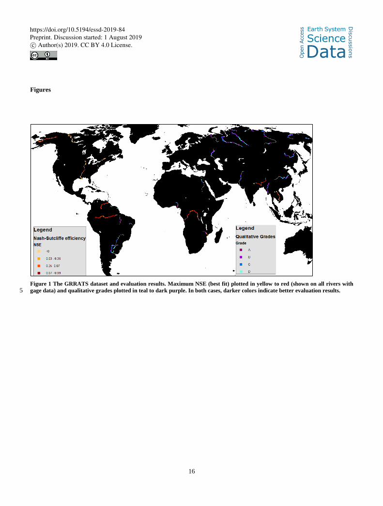
GRRATS processing produced a total of 932 globally distributed virtual stations (Figure 1). The 39 GRRATS rivers account
for 50.M km2 (>34%) of global drainage area, and include 13 Arctic rivers. To attain these results, we extracted and
processed a total of 1.5M individual radar returns at 1478 potential VS locations.
3.1 Filtering returns
We removed 309.7K altimetry returns with our height filters (steps 1 and 2 of our filtering process), leaving 1.1M (78.2%) 25
viable measurements. Our ice filter removed an additional 296.9K of the remaining returns (step 3) resulting in 810.4K
viable returns (57.2%). Averaging all height returns within the river polygons for each pass at each VS (step 4) led to a total
of 102.3K (21.9K on Arctic rivers) pass-averaged measurements. VS were required to retain 50% (without ice) or 25% (with
ice) of their passes post-filtering to be included in the final data product, resulting in the removal of 465 potential VS
locations (step 5). VS were also removed by visual inspection if they were tidal, resulting in the removal of an additional 45 30
stations (step 6). While many VS were filtered heavily, 72.8% of the total returns for all VS in the final product passed all
https://doi.org/10.5194/essd-2019-84
Ope
n A
cces
s Earth System
Science
DataD
iscussio
ns
Preprint. Discussion started: 1 August 2019c© Author(s) 2019. CC BY 4.0 License.
7
filters (the median VS value being 97.7%) and 227 VS lost no returns. The filtering process resulted in a total 932 VS for
evaluation derived from standard retracked data (ICE 1). These VS had a data set wide average of ~16 measurements per
year (9.5 for Envisat VS and 35.8 for Jason2 VS).
3.2 Example Time Series evaluation
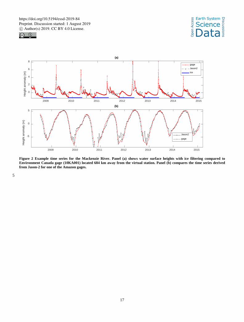
Figure 2 shows example GRRATS time series for the Mackenzie and Amazon Rivers and corresponding in-situ gages. 5
Comparison between the Jason-2 time series and the gage on the Mackenzie River produced STDE = 0.5 m, NSE = 0.41, and
an R = 0.64. In this case, the gage used for evaluation was located ~700 km upriver (Figure 2(a)). The STDE is
approximately consistent with what is expected from the literature (Asadzadeh Jarihani et al., 2013; Frappart et al., 2006).
However, the STDE is relatively large in comparison with the overall annual range in the time series (typically ~2 m)
observed from the gage (see Figure 2 (a)), leading to a relatively low NSE. Additionally, several cycles have far larger 10
errors, reaching up to two meters, in some cases. There are a total of 3 in-situ gages used for evaluation on the Mackenzie
River. Across the 3 gage comparisons, this VS had median statistics of 0.58 m, 0.35 and 0.64 for STDE, NSE, and R,
respectively. Comparing the VS data to the gage on the Amazon River yields STDE= 0.98 m, NSE= 0.94 and R= 0.97, with
the evaluation gage 263 km upriver from the VS (Figure 2(b)). Despite the STDE being nearly twice as large, the magnitude
of change on the Amazon allowed for a much better fit due to the large interannual variability of the Amazon floodwave 15
(>10 m). Most of the error was from times of low flow near the ends of the calendar year in 2009, 2011 and 2012. There are
6 in-situ gages on the Amazon River. Across these comparisons, this VS had median statistics of 0.94 m, 0.95, and 0.98 for
STDE, NSE, and R, respectively.
3.3 GRRATS evaluation across all rivers
We compared GRRATS against in-situ evaluation data on a total of 12 rivers. This provided evaluation of 380 of the 920 20
virtual stations (42%). On each river, the total number of time series evaluations was the product of the number of VS and
the number of gages (Figure 1). Thus, the total number of time series evaluations (summed across all 12 rivers) was 1,915.
A total of 72.5% of the quantitatively evaluated virtual stations had an NSE greater than 0.4 when compared with at least one
gage. The highest maximum NSE (Figure 3(a)) was 0.98, from an Envisat VS in the upper reaches of the Amazon. The
median value for maximum NSEs for all VS was 0.75 (0.67 from closet gage comparison Figure 3(i)). A total of 341 of the 25
389 (87.7 %) virtual stations had a maximum NSE >0 (Figure 3(e)) .The highest median NSE (Figure 3(b) and Figure 3(f))
values were 0.96 at two Envisat VS on the Orinoco river (lower and mid). A total of 277 of 389 (71.2%) had a mean NSE
>0.
The smallest minimum STDE (to two significant digits) was 0.11 m and occurred at an Envisat VS on the upper Congo. The
median value for minimum STDE (Figure 3C) for all VS was 0.93 m (1.08m from closest gage comparison Figure 3(j)). The 30
minimum and median value for median STDE (Figure 3(d)) were 0.31 m, and 1.3 m respectively. Our STDE error statistics
are greater than previous work reporting accuracies ranging from 0.14 m to 0.43 m for Envisat data and 0.19 m to 0.31 m for
https://doi.org/10.5194/essd-2019-84
Ope
n A
cces
s Earth System
Science
DataD
iscussio
ns
Preprint. Discussion started: 1 August 2019c© Author(s) 2019. CC BY 4.0 License.

8
Jason-2 data (Frappart et al., 2006; Kuo & Kao, 2011; Papa et al., 2012; Santos da Silva et al., 2010). This discrepancy is
likely because GRRATS includes VS on rivers where evaluations have not previously been reported in the literature, and the
fact that we do not fine-tune processing or filtering to each VS due to the global nature of the dataset.
Some locations with relatively low STDE values showed poor performance in terms of NSE, particularly for rivers with
relatively low water elevation variability. VS on the St Lawrence River had minimum STDE ranging from 0.58 - 3.27 m. 5
The VS with 0.58 m STDE corresponded with a maximum NSE value of -0.27, indicating quite poor performance in
resolving river variations (standard deviation of 0.35 m). The St Lawrence River is anomalous in other ways as well. For 2
potential VS (one each from Jason 2 and Envisat), the unprocessed data (ICE-1 retracked GDR data) showed a bias of
several tens of meters above the baseline height, and thus no data for these VS are included in GRRATS. Closer examination
of these VS seems to indicate that the on-board tracking window was often tens of meters outside of the river surface range, 10
making retrievals from the surface impossible. This case is particularly odd as such errors are not expected for wider rivers;
the St Lawrence is between 2 and 7 km wide where we sampled it. Such errors are more commonly associated with altimeter
returns from near-river topography on narrow rivers (Biancamaria et al., 2017; Frappart et al., 2006; Maillard et al., 2015;
Santos da Silva et al., 2010). Moderately poor performance from the remainder of VS in terms of NSE and STDE on the
river is likely due to the river lacking enough variation in height to allow for retrieval of a good signal outside the error range 15
of radar altimeters. However, this low variation data can still be quite useful to modelers for determining if their results show
excessive change in the annual cycle of water elevations.
The median of the maximum R values (Figure 3(g)) for each station is 0.9 (0.87 from closest gage comparison Figure 3(k)).
The maximum R value plot shows left skewness, similar to the NSE results. The lowest maximum R value of -0.15 occurred
at an Envisat VS on the mid St Lawrence River, which was the only virtual station to display a negative correlation. The best 20
maximum R value was 0.99 for an Envisat station near the mouth of the Ganges River that also displayed high NSE and low
STDE. The median value of the median R (Figure 3(h)) is 0.69. The values range from -0.18 (an Envisat VS on the lower St
Lawrence) to 0.99 (an Envisat VS on the lower Brahmaputra).
For 27 of the 39 rivers in the GRRATS dataset, no in-situ data is available for evaluation. We gave the remaining 27 rivers
qualitative letter grades based on number of missing data points, obvious outliers, and agreement with nearby stations. These 25
grades are included with the data for end users.
3.4 Towards quantitative performance prediction
As is evident above, radar altimeter performance varies dramatically across rivers and across VS. Generally, measurements
from wide rivers without large topographic features in the altimeter footprints that have large seasonal water elevation
variations tend to result in better altimeter performance. In order to identify conditions that may contribute to poor return 30
quality, we compared both VS width and percentage of original returns post-filtering, near-river topography, and river height
variation with all three fit statistics. We found no statistically significant relationships in this evaluation, a finding that
supports existing literature on quantitative prediction of altimeter performance (Maillard et al., 2015). Indeed, we found
https://doi.org/10.5194/essd-2019-84
Ope
n A
cces
s Earth System
Science
DataD
iscussio
ns
Preprint. Discussion started: 1 August 2019c© Author(s) 2019. CC BY 4.0 License.

9
many examples of counterintuitive performance in our examination. The St. Lawrence (described above) is an example of
unexpectedly poor performance; typical predictors such as width (smallest VS ~1.5 km wide) and the lack of extreme
proximal topography led to an expectation of accurate performance that was not met. Meanwhile, other rivers defied the
normal pattern by showing good fit metrics while being far narrower. The Mississippi River was consistently at our lower
limit for river width. The VS widths ranged from 509.1 m to 2,608.0 m, and had an average width of just 955.3 m. The 5
average near-river relief ranged from 10-60 m. The Mississippi maximum NSE values ranged from -0.22 to 0.96, with an
average of 0.43. Minimum STDE values ranged from 0.34 m-2.22 m, with an average of 1.18 m. additionally, we computed
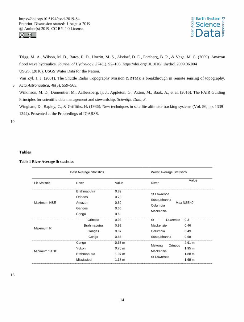
average error statistics across all VS along each river. Some rivers stood out as particularly good or poor performers (Table
1), but no broad geographical patterns emerged. For this reason, we recommend using the median (dataset wide) value for
evaluated STDE (0.93 m) as an error estimate for VS without evaluation data, as this is representative of 42% of all of the 10
VS in the dataset. We suggest that individual VS data point error be estimated as the STDE of the time series they are a
component of.
3.5 Comparison to other altimetry datasets
While it is outside the scope of this study to compare GRRATS exhaustively with existing datasets, we find it appropriate to
demonstrate that our dataset is comparable. Therefore, we compared two VS locations that are in each of the four datasets 15
discussed (one on the Amazon, one on the Congo). Figure 4 (a-c) show time series anomaly at each VS and the closest gage.
Note that time series lengths are limited to the shortest time series in the comparison and do not match the coverage of any
particular mission. GRRATS, DAHITI, and Hydroweb are similar and fit with the in-situ gage well (Table 2). DAHITI is
missing data on the Amazon time series. HydroSat and River&LakeNRT are frequently out of phase, particularly on the
Amazon River (Figure 4(a)). Performance is similar on ungaged rivers when compared (Figure 5). GRRATS and DAHITI 20
showed good agreement on the Parana River (Figure 5(a)). HydroSat and Hydroweb (Figure 5(b-c)), are differentiated from
GRRATS on the Ob’ and Lena Rivers, as they show heights from a frozen river that GRRATS flags and removes. During
overlap, HydroSat and GRRATS were similar at the Ob’ VS. Hydroweb data on the Lena is similar to GRRATS, with the
exception of the 2006 peak flow, which is missing. Note that much of the rising limb is missing in these time series as it
occurs during times of ice cover. Unfiltered data and ice flags are available to data users if needed. This process 25
demonstrated that our quasi-automated methods produce a dataset with global coverage and performance that approximates
the accuracy of regional altimetry datasets.
4. Data availability
GRRATS (DOI 10.5067/PSGRA-SA2V1) is available at ftp://podaac-ftp.jpl.nasa.gov/allData/preswot_hydrology/L2/rivers
for non-commercial use only (Durand et al., 2016). An interactive map of the data is located at 30
http://research.bpcrc.osu.edu/grrats/
https://doi.org/10.5194/essd-2019-84
Ope
n A
cces
s Earth System
Science
DataD
iscussio
ns
Preprint. Discussion started: 1 August 2019c© Author(s) 2019. CC BY 4.0 License.

10
5. Conclusion
We find that uniform altimeter data processing produces usable data with accessible documentation for end users.
Encouraging end user understanding of how this kind of data is produced is critical in fostering its use across the scientific
and stakeholder communities. GRRATS considers only ocean-draining (highest order) rivers, while other datasets include
some VS on large tributaries. However, our use of the GRWL dataset allowed for a comprehensive selection of altimeter 5
crossings on a global scale. These features should enable broad use by the scientific community. This resulted in GRRATS
having the best coverage available for North American rivers as well. We produced GRRATS with ease of use in mind. VS
metadata are included and the product can be downloaded in bulk.
On the whole, the median value of the error standard deviation is 0.93 m, which is similar to or slightly larger than values
reported for the rivers that are most commonly studied using radar altimetry (e.g., the Amazon and Congo). Our philosophy 10
in constructing the dataset was to maximize the spatial coverage of altimeter crossings, construct the product in a uniform
way, and to provide an evaluation of quality for each VS. Thus, users can decide whether each VS is useful given their data
needs. Note that a total of 77.2% of virtual stations evaluated against in-situ data had an NSE>0.4. Our uniform production
method allowed us to evaluate whether river width or the height of bluffs proximal to rivers at altimeter crossings correlate
with altimeter performance, as was expected in the literature. However, we were unable to identify a predictive model for 15
altimeter performance, and leave this exercise for future work.
The GRRATS dataset maximizes traceability: all of the information needed to re-process these VS is included in the final
data product. It is our expectation that other researchers could implement other methods of filtering and processing to
achieve derived data products tailored to their applications.
Author Contributions 20
SC1 developed and finalized processing algorithms, performed methods exploration, was primary data manager, analyzed
final product, and finalized manuscript. MD developed algorithms, performed quality analysis, and provided editorial and
graphical assistance. YY performed GDR extraction and geodetic corrections and was primary unprocessed data manager.
YJ performed methods exploration. QG performed methods exploration. ST developed algorithms and performed methods
exploration. CKS provided technical expertise and editorial assistance. GHA and TP provided access to GRWL width data 25
used to find virtual station targets. SC2 provided technical expertise, in situ data, and editorial assistance.
Acknowledgments
This work was produced on behalf of the NASA MEaSUREs group (grants NNX13AK45A, and NNX15AH05A). We
would like to acknowledge the use of stream gage data and imagery obtained from the USGS stream gage network and other
organizations, and USGS Landsat archive, respectively; as well as altimeter VS data products from other research institutes. 30
https://doi.org/10.5194/essd-2019-84
Ope
n A
cces
s Earth System
Science
DataD
iscussio
ns
Preprint. Discussion started: 1 August 2019c© Author(s) 2019. CC BY 4.0 License.
11
References
Abrams, M. (2000). The Advanced Spaceborne Thermal Emission and Reflection Radiometer (ASTER): data products for
the high spatial resolution imager on NASA’s Terra platform. International Journal of Remote Sensing, 21(5), 847–859.
Allen, G. H., & Pavelsky, T. M. (2015). Characterizing worldwide patterns of fluvial geomorphology and hydrology with the
Global River Widths from Landsat (GRWL) database. Presented at the AGU Fall Meeting Abstracts. 5
Allen, G. H., & Pavelsky, T. M. (2018). Global extent of rivers and streams. Science, 361(6402), 585.
https://doi.org/10.1126/science.aat0636
Alsdorf, D., Rodríguez, E., & Lettenmaier, D. P. (2007). Measuring surface water from space. Reviews of Geophysics, 45(2),
n/a-n/a. https://doi.org/10.1029/2006RG000197
Asadzadeh Jarihani, A., Callow, J. N., Johansen, K., & Gouweleeuw, B. (2013). Evaluation of multiple satellite altimetry 10
data for studying inland water bodies and river floods. Journal of Hydrology, 505, 78–90.
https://doi.org/10.1016/j.jhydrol.2013.09.010
Berry, P. (2010). Monitoring of inland surface water using multi-mission satellite radar altimetry.
Biancamaria, S., Frappart, F., Leleu, A.-S., Marieu, V., Blumstein, D., Desjonquères, J.-D., et al. (2017). Satellite radar
altimetry water elevations performance over a 200 m wide river: Evaluation over the Garonne River. Advances in Space 15
Research, 59(1), 128–146. https://doi.org/10.1016/j.asr.2016.10.008
Biancamaria, S., Schaedele, T., Blumstein, D., Frappart, F., Boy, F., Desjonquères, J.-D., et al. (2018). Validation of Jason-3
tracking modes over French rivers. Remote Sensing of Environment, 209, 77–89. https://doi.org/10.1016/j.rse.2018.02.037
Birkett, C. M., Mertes, L., Dunne, T., Costa, M., & Jasinski, M. (2002). Surface water dynamics in the Amazon Basin:
Application of satellite radar altimetry (DOI 10.1029/2001JD000609). JOURNAL OF GEOPHYSICAL RESEARCH-ALL 20
SERIES-, 107(20; SECT 4), LBA-26.
Bjerklie, D. M., Moller, D., Smith, L. C., & Dingman, S. L. (2005). Estimating discharge in rivers using remotely sensed
hydraulic information. Journal of Hydrology, 309(1), 191–209.
Calmant, S., & Seyler, F. (2006). Continental surface waters from satellite altimetry. Comptes Rendus Geoscience, 338(14),
1113–1122. 25
Calmant, S., Seyler, F., & Cretaux, J. F. (2008). Monitoring continental surface waters by satellite altimetry. Surveys in
Geophysics, 29(4–5), 247–269.
Danielson, J. J., & Gesch, D. B. (2011). Global multi-resolution terrain elevation data 2010 (GMTED2010) (Report No.
2011–1073). Retrieved from http://pubs.er.usgs.gov/publication/ofr20111073
Dumont, J., Rosmorduc, V., Picot, N., Desai, S., Bonekamp, H., Figa, J., et al. (2009). OSTM/Jason-2 products handbook. 30
CNES: SALP-MU-M-OP-15815-CN, EUMETSAT: EUM/OPS-JAS/MAN/08/0041, JPL: OSTM-29-1237, NOAA/NESDIS:
Polar Series/OSTM J, 400, 1.
https://doi.org/10.5194/essd-2019-84
Ope
n A
cces
s Earth System
Science
DataD
iscussio
ns
Preprint. Discussion started: 1 August 2019c© Author(s) 2019. CC BY 4.0 License.
12
Durand, M., Coss, Stephen, & Lettenmaier, Denis. (2016). Pre SWOT Hydrology GRRATS Jason-2 Virtual Station Heights
Version 1. Ver. 1. PO.DAAC (ftp://podaac-ftp.jpl.nasa.gov/allData/preswot_hydrology/L2/rivers).
https://doi.org/10.5067/PSGRA-SA2V1
Environment Canada. (2016). Surface water data. Inland Waters Directorate, Water Resources Branch, Water Survey of
Canada, Ottawa. 5
Frappart, F., Calmant, S., Cauhopé, M., Seyler, F., & Cazenave, A. (2006). Preliminary results of ENVISAT RA-2-derived
water levels validation over the Amazon basin. Remote Sensing of Environment, 100(2), 252–264.
https://doi.org/10.1016/j.rse.2005.10.027
Gommenginger, C., Thibaut, P., Fenoglio-Marc, L., Quartly, G., Deng, X., Gómez-Enri, J., et al. (2011). Retracking
Altimeter Waveforms Near the Coasts. In S. Vignudelli, A. G. Kostianoy, P. Cipollini, & J. Benveniste (Eds.), Coastal 10
Altimetry (pp. 61–101). Berlin, Heidelberg: Springer Berlin Heidelberg. https://doi.org/10.1007/978-3-642-12796-0_4
Hannah, D. M., Demuth, S., van Lanen, H. A., Looser, U., Prudhomme, C., Rees, G., et al. (2011). Large‐scale river flow
archives: importance, current status and future needs. Hydrological Processes, 25(7), 1191–1200.
Huang, Q., Long, D., Du, M., Zeng, C., Li, X., Hou, A., & Hong, Y. (2018). An improved approach to monitoring
Brahmaputra River water levels using retracked altimetry data. Remote Sensing of Environment, 211, 112–128. 15
https://doi.org/10.1016/j.rse.2018.04.018
Jacobs, J. W. (2002). The Mekong River Commission: transboundary water resources planning and regional security.
Geographical Journal, 168(4), 354–364.
Jung, H. C., Hamski, J., Durand, M., Alsdorf, D., Hossain, F., Lee, H., et al. (2010). Characterization of complex fluvial
systems using remote sensing of spatial and temporal water level variations in the Amazon, Congo, and Brahmaputra Rivers. 20
Earth Surface Processes and Landforms, 35(3), 294–304.
Kuo, C.-Y., & Kao, H.-C. (2011). Retracked Jason-2 Altimetry over Small Water Bodies: Case Study of Bajhang River,
Taiwan. Marine Geodesy, 34(3–4), 382–392. https://doi.org/10.1080/01490419.2011.584830
Maillard, P., Bercher, N., & Calmant, S. (2015). New processing approaches on the retrieval of water levels in Envisat and
SARAL radar altimetry over rivers: A case study of the São Francisco River, Brazil. Remote Sensing of Environment, 156, 25
226–241. https://doi.org/10.1016/j.rse.2014.09.027
Martinez, J.-M. (2003, January 1). SO HYBAM. Retrieved December 6, 2016, from www.ore-hybam.org
Michailovsky, C., McEnnis, S., Berry, P., Smith, R., & Bauer-Gottwein, P. (2012). River monitoring from satellite radar
altimetry in the Zambezi River basin. Hydrology and Earth System Sciences, 16(7), 2181–2192.
Oki, K., & Yasuoka, Y. (2008). Mapping the potential annual total nitrogen load in the river basins of Japan with remotely 30
sensed imagery. Remote Sensing of Environment, 112(6), 3091–3098.
Overton, I. C. (2015). Modelling floodplain inundation on a regulated river: integrating GIS, remote sensing and
hydrological models. River Research and Applications, 21(9), 991–1001. https://doi.org/10.1002/rra.867
https://doi.org/10.5194/essd-2019-84
Ope
n A
cces
s Earth System
Science
DataD
iscussio
ns
Preprint. Discussion started: 1 August 2019c© Author(s) 2019. CC BY 4.0 License.

13
Papa, F., Prigent, C., Aires, F., Jimenez, C., Rossow, W., & Matthews, E. (2010). Interannual variability of surface water
extent at the global scale, 1993–2004. Journal of Geophysical Research: Atmospheres, 115(D12).
Papa, F., Bala, S. K., Pandey, R. K., Durand, F., Gopalakrishna, V. V., Rahman, A., & Rossow, W. B. (2012). Ganga-
Brahmaputra river discharge from Jason-2 radar altimetry: An update to the long-term satellite-derived estimates of
continental freshwater forcing flux into the Bay of Bengal. Journal of Geophysical Research: Oceans, 117(C11), n/a–n/a. 5
https://doi.org/10.1029/2012JC008158
Pavelsky, T. M., & Smith, L. C. (2004). Spatial and Temporal Patterns in Arctic River Ice Breakup Observed with Modis
and Avhrr Time Series. Remote Sensing of Environment, 93(3), 328–338.
Pavelsky, T. M., Durand, M. T., Andreadis, K. M., Beighley, R. E., Paiva, R. C. D., Allen, G. H., & Miller, Z. F. (2014).
Assessing the potential global extent of SWOT river discharge observations. Journal of Hydrology, 519, Part B, 1516–1525. 10
https://doi.org/10.1016/j.jhydrol.2014.08.044
Pavlis, N. K., Holmes, S. A., Kenyon, S. C., & Factor, J. K. (2012). The development and evaluation of the Earth
Gravitational Model 2008 (EGM2008). Journal of Geophysical Research: Solid Earth, 117(B4), n/a–n/a.
https://doi.org/10.1029/2011JB008916
Sampson, C. C., Smith, A. M., Bates, P. D., Neal, J. C., Alfieri, L., & Freer, J. E. (2015). A high‐resolution global flood 15
hazard model. Water Resources Research, 51(9), 7358–7381.
Santos da Silva, J., Calmant, S., Seyler, F., Rotunno Filho, O. C., Cochonneau, G., & Mansur, W. J. (2010). Water levels in
the Amazon basin derived from the ERS 2 and ENVISAT radar altimetry missions. Remote Sensing of Environment,
114(10), 2160–2181. https://doi.org/10.1016/j.rse.2010.04.020
Schumann, G., Bates, P. D., Apel, H., & Aronica, G. T. (2018). Global Flood Hazard Mapping, Modeling, and Forecasting: 20
Challenges and Perspectives. Global Flood Hazard: Applications in Modeling, Mapping, and Forecasting, 239–244.
Schwatke, C., Dettmering, D., Bosch, W., & Seitz, F. (2015). DAHITI–an innovative approach for estimating water level
time series over inland waters using multi-mission satellite altimetry. Hydrology and Earth System Sciences, 19(10), 4345–
4364.
Shiklomanov, A. I., Lammers, R., & Vörösmarty, C. J. (2002). Widespread decline in hydrological monitoring threatens 25
pan‐Arctic research. Eos, Transactions American Geophysical Union, 83(2), 13–17.
Smith, A., Sampson, C., & Bates, P. (2015). Regional flood frequency analysis at the global scale. Water Resources
Research, 51(1), 539–553.
Soussi, B., & Féménias, P. (2009). ENVISAT ALTIMETRY Level 2 User Manual, (1.3). Retrieved from
https://earth.esa.int/c/document_library/get_file?folderId=38553&name=DLFE-688.pdf 30
Sulistioadi, Y. B., Tseng, K. H., Shum, C. K., Hidayat, H., Sumaryono, M., Suhardiman, A., et al. (2015). Satellite radar
altimetry for monitoring small rivers and lakes in Indonesia. Hydrology and Earth System Sciences, 19(1), 341–359.
Tourian, M., Tarpanelli, A., Elmi, O., Qin, T., Brocca, L., Moramarco, T., & Sneeuw, N. (2016). Spatiotemporal
densification of river water level time series by multimission satellite altimetry. Water Resources Research.
https://doi.org/10.5194/essd-2019-84
Ope
n A
cces
s Earth System
Science
DataD
iscussio
ns
Preprint. Discussion started: 1 August 2019c© Author(s) 2019. CC BY 4.0 License.
14
Trigg, M. A., Wilson, M. D., Bates, P. D., Horritt, M. S., Alsdorf, D. E., Forsberg, B. R., & Vega, M. C. (2009). Amazon
flood wave hydraulics. Journal of Hydrology, 374(1), 92–105. https://doi.org/10.1016/j.jhydrol.2009.06.004
USGS. (2016). USGS Water Data for the Nation.
Van Zyl, J. J. (2001). The Shuttle Radar Topography Mission (SRTM): a breakthrough in remote sensing of topography.
Acta Astronautica, 48(5), 559–565. 5
Wilkinson, M. D., Dumontier, M., Aalbersberg, Ij. J., Appleton, G., Axton, M., Baak, A., et al. (2016). The FAIR Guiding
Principles for scientific data management and stewardship. Scientific Data, 3.
Wingham, D., Rapley, C., & Griffiths, H. (1986). New techniques in satellite altimeter tracking systems (Vol. 86, pp. 1339–
1344). Presented at the Proceedings of IGARSS.
10
Tables
Table 1 River Average fit statistics
Best Average Statistics Worst Average Statistics
Fit Statistic River Value River Value
Maximum NSE
Brahmaputra
Orinoco
Amazon
Ganges
Congo
0.82
0.78
0.69
0.65
0.6
St Lawrence
Susquehanna
Columbia
Mackenzie
Max NSE<0
Maximum R
Orinoco
Brahmaputra
Ganges
Congo
0.93
0.92
0.87
0.85
St Lawrence
Mackenzie
Columbia
Susquehanna
0.3
0.46
0.49
0.68
Minimum STDE
Congo
Yukon
Brahmaputra
Mississippi
0.53 m
0.76 m
1.07 m
1.18 m
Mekong Orinoco
Mackenzie
St Lawrence
2.61 m
1.95 m
1.88 m
1.69 m
15
https://doi.org/10.5194/essd-2019-84
Ope
n A
cces
s Earth System
Science
DataD
iscussio
ns
Preprint. Discussion started: 1 August 2019c© Author(s) 2019. CC BY 4.0 License.

15
Table 2 Multi-product fist statistics from figure 5
Product STDE R NSE
Amazon River
HydroSat 2.12 m 0.61 0.33
Hydroweb 1.42 m 0.96 0.72
NRTRL 2.9 m 0.3 -0.74
DAHITI 0.85 m 0.99 0.81
GRRATS 1.57 m 0.95 0.65
Congo River
HydroSat 0.48 m 0.87 0.76
Hydroweb 0.42 m 0.92 0.84
NRTRL 3.2 m 0.11 -7.88
DAHITI 0.39 m 0.93 0.86
GRRATS 0.5 m 0.91 0.81
Brahmaputra River
HydroSat 0.56 m 0.96 0.92
Hydroweb 0.58 m 0.91 0.96
DAHITI 0.6 m 0.96 0.86
GRRATS 0.69 m 0.95 0.87
https://doi.org/10.5194/essd-2019-84
Ope
n A
cces
s Earth System
Science
DataD
iscussio
ns
Preprint. Discussion started: 1 August 2019c© Author(s) 2019. CC BY 4.0 License.
16
Figures
Figure 1 The GRRATS dataset and evaluation results. Maximum NSE (best fit) plotted in yellow to red (shown on all rivers with gage data) and qualitative grades plotted in teal to dark purple. In both cases, darker colors indicate better evaluation results. 5
https://doi.org/10.5194/essd-2019-84
Ope
n A
cces
s Earth System
Science
DataD
iscussio
ns
Preprint. Discussion started: 1 August 2019c© Author(s) 2019. CC BY 4.0 License.
17
Figure 2 Example time series for the Mackenzie River. Panel (a) shows water surface heights with ice filtering compared to Environment Canada gage (10KA001) located 684 km away from the virtual station. Panel (b) compares the time series derived from Jason-2 for one of the Amazon gages.
5
2009 2010 2011 2012 2013 2014 2015
0
2
4
6
8
Hei
ght a
nom
aly
(m)
(a)
gageJason2ice
2009 2010 2011 2012 2013 2014 2015
-5
0
5
Hei
ght a
nom
aly
(m)
(b)
Jason2
gage
https://doi.org/10.5194/essd-2019-84
Ope
n A
cces
s Earth System
Science
DataD
iscussio
ns
Preprint. Discussion started: 1 August 2019c© Author(s) 2019. CC BY 4.0 License.

18
Figure 3 Virtual Stations Nash-Sutcliffe efficiencies computed with all available evaluation gages located in the same river. Panel (a) histogram of the max NSE at each VS in the dataset, Panel (b) histogram of the median NSE at each VS in the dataset, Panel (c) histogram of the minimum STDE at each VS in the dataset, Panel (d) A histogram of the median STDE in the dataset, Panel (e) A 5 histogram of the Max NSE at all theVS in the dataset with NSE>0,Panel (f) histogram of the median NSE at at all theVS in the dataset with NSE>0, Panel (g) histogram of the max R at each VS in the dataset, Panel (h) histogram of the median R at each VS in the dataset, Panel (i) histogram of closest STDE, Panel (j) histogram of closest NSE>0, Panel (k) histogram of closest R.
(a)
-40 -20 0
Max NSE
0
100
200
300
400
coun
t
(b)
-200 -150 -100 -50 0
Median NSE
0
50
100
150
200
250
300
(e)
0 0.5 1
Max NSE>0
0
50
100
150
coun
t
(f)
0 0.5 1
Median NSE>0
0
10
20
30
40
50
(c)
0 2 4 6
Min STDE (m)
0
20
40
60
80
100
120(d)
0 2 4 6
Median STDE (m)
0
50
100
150
(g)
0 0.5 1
Max R
0
50
100
150
200 (h)
0 0.5 1
Medain R
0
20
40
60
80
100
(i)
0 2 4 6
Closest STDE (m)
0
20
40
60
80
100
coun
t
(k)
0 0.5 1
Closest R
0
50
100
150
200(j)
0 0.5 1
Closest NSE >0
0
20
40
60
80
100
https://doi.org/10.5194/essd-2019-84
Ope
n A
cces
s Earth System
Science
DataD
iscussio
ns
Preprint. Discussion started: 1 August 2019c© Author(s) 2019. CC BY 4.0 License.

19
Figure 4: Multi product evaluation at same location. Panel (a): multiproduct comparison on the Amazon River Panel (b): multi product comparison on the Congo River. Panel (c): multi product comparison on Brahmaputra River. DAHITI plotted in purple with square markers, HydroSat in dark blue with circle markers, River&LakeNRT in yellow with diamond markers, Hydroweb in red with cross markers, and GRRATS in green with x markers and in-situ in dashed light blue. 5
10
2010 2011 2012 2013
-5
0
5
heig
ht a
nom
alie
s (m
)
(a)
Q3-08 Q4-08 Q1-09 Q2-09 Q3-09 Q4-09 Q1-10
-6
-4
-2
0
2
heig
ht a
nom
alie
s (m
)
(b)
2011 2012 2013 2014
-4
-2
0
2
4
heig
ht a
nom
alie
s (m
)
(c)
https://doi.org/10.5194/essd-2019-84
Ope
n A
cces
s Earth System
Science
DataD
iscussio
ns
Preprint. Discussion started: 1 August 2019c© Author(s) 2019. CC BY 4.0 License.

20
Figure 5 multi product evaluation at ungagged river locations GRRATS plotted in green, DAHITI in purple with square markers, HydroSat in blue with circle markers, HydroWeb in red with cross markers, and times of ice cover plotted with a dotted black line. Panel (a) is a comparison with DAHITI on the Parana River. Panel (b) is a comparison with HydroSat on the Ob River, and 5 Panel (c) is a comparison with HydroWeb on the Lena River.
10
2008 2009 2010 2011 2012 2013 2014 2015 2016 2017-2
-1
0
1
2
heig
ht
anom
alie
s (m
)
(a)
2008 2009 2010 2011 2012 2013 2014 2015 2016-4
-2
0
2
4
heig
ht
anom
alie
s (m
)
(b)
2003 2004 2005 2006 2007 2008 2009 2010
-2
0
2
4
heig
ht
anom
alie
s (m
)
(c)
https://doi.org/10.5194/essd-2019-84
Ope
n A
cces
s Earth System
Science
DataD
iscussio
ns
Preprint. Discussion started: 1 August 2019c© Author(s) 2019. CC BY 4.0 License.