essential mathematics for games - cap 8 lighting.pdf

Chapter8Lighting

8.1 Introduction

Much of the way we perceive the world visually is based on the way objectsin the world react to the light around them. This is especially true when thelighting around us is changing or the lights or objects are moving. Given thesefacts, it is not surprising that one of the most common uses of programmableshading is to simulate the appearance of real-world lighting.The coloring methods we have discussed so far have used colors that are

statically assigned at content creation time (by the artist) or at the start of theapplication. These colors do not change on a frame-to-frame basis. At best,these colors represent a “snapshot” of the scene lighting at a given momentfor a given configuration of objects. Even if we only intend to model sceneswhere the lights and objects remain static, these static colors cannot repre-sent the view-dependent nature of lighting with respect to shiny or glossysurfaces.Clearly, we need a dynamic method of rendering lighting in real time.

At the highest level, this requires two basic items: a mathematical model forcomputing the colors generated by lighting and ahigh-performancemethod ofimplementing this model. We have already introduced the latter requirement;programmable shading pipelines were designed specifically with geometricand color computations (such as lighting) in mind. In this chapter we willgreatly expand upon the basic shaders, data sources, and shader syntax thatwere introduced in Chapter 7. However, we must first address the otherrequirement— the mathematical model we will use to represent lighting.The following sections will discuss the details of a popular set of meth-

ods for approximating lighting for real-time rendering, as well as examplesof how these methods can be implemented as shaders. While we will use

315

316 Chapter 8 Lighting

shaders to implement them, the lighting model we will discuss is basedupon the long-standing OpenGL fixed-function lighting pipeline (introducedin OpenGL 1.x). At the end of the chapter we will introduce several moreadvanced lighting techniques that take advantage of the unique abilities ofprogrammable shaders.

We will refer to fixed-function lighting pipelines in many places in thischapter. Fixed-function lighting pipelines were the methods used in ren-dering application programming interfaces (APIs) to represent lighting cal-culations prior to the availability of programmable shaders. They are calledfixed-function pipelines because the only options available to users of thesepipelines were to change the values of predefined colors and settings. Thepipelines implemented a basically fixed-structure lighting equation and pre-sented a limited, fixed set of options to the application programmer. No othermodifications to the lighting pipeline (and thus the lighting equation or rep-resentation) were available. Shaders make it possible to implement the exactlighting methods desired by the particular application.

8.2 Basics of Light Approximation

The physical properties of light are incredibly complex. Even relatively simplescenes never could be rendered realistically without “cheating.” In a sense, allof computer graphics is little more than cheating—finding the cheapest-to-compute approximation for a given situation that will still result in a realisticimage. Even non-real-time, photorealistic renderings are only approximationsof reality, trading off accuracy for ease and speed of computation.

Real-time renderings are even more superficial approximations. Light inthe real world reflects, scatters, refracts, and otherwise bounces around theenvironment. Historically, real-time three-dimensional (3D) lighting oftenmodeled only direct lighting, the light that comes along an unobstructedpath from light source to surface. Worse yet, many legacy real-time lightingsystems (such as OpenGL and Direct3D’s fixed-function lighting pipelines)do not support automatic shadowing. Shadowing involves computing light-blocking effects from objects located between the object being lit and the lightsource. These are ignored in the name of efficiency. However, despite theselimitations, even basic lighting can have a tremendous impact on the overallimpression of a rendered 3D scene.

Lighting in real-time 3D generally involves data from at least threedifferent sources: the surface configuration (vertex position, normal vector),surface material (how the surface reacts to light), and light emitter properties(the way the light sources emit light). We will discuss each of these sources interms of how they affect the lighting of an object and will then discuss howthese values are passed to the shaderswewill be constructing. All of the shaderconcepts from Chapter 7 (vertex and fragment shading, attributes, uniformsand varying, etc.) will be pivotal in our creation of a lighting system.

8.2 Basics of Light Approximation 317

8.2.1 Measuring Light

In order to understand the mathematics of lighting, even the simplified,nonphysical approximation used by most real-time 3D systems, it is help-ful to know more about how light is actually measured. The simplest way toappreciate how we measure light is in terms of an idealized lightbulb andan idealized surface being lit by that bulb. To explain both the brightnessand luminance (these are actually two different concepts; we will define themin the following section) of a lit surface, we need to measure and track thefollowing path from end to end:

� The amount of light generated by the bulb.

� The amount of light reaching the surface from the bulb.

� The amount of light reaching the viewer from the surface.

Each of these is measured and quantified differently. First, we need a way ofmeasuring the amount of light being generated by the lightbulb. Lightbulbsare generally rated according to several different criteria. The number mostpeople think of with respect to lightbulbs is wattage. For example, we think ofa 100-watt lightbulb as beingmuch brighter than a 25-watt lightbulb, and thisis generally true when comparing bulbs of the same kind. Wattage in this caseis a measure of the electrical power consumed by the bulb in order to createlight. It is not a direct measure of the amount of light actually generated bythe bulb. In other words, two lightbulbs may consume the same wattage (say,100 watts) but produce different amounts of light—one type of bulb simplymay bemore efficient at converting electricity to light. So what is the measureof light output from the bulb?

Overall light output from a light source is ameasure of power: light energyper unit time. This quantity is called luminous flux. The unit of luminous fluxis the lumen. The luminous flux from a lightbulb is measured in lumens, aquantity that is generally listed on boxes of commercially available lightbulbs,near thewattage rating.However, lumens are not howwemeasure the amountof light that is incident upon a surface.

There are several different ways of measuring the light incident upon asurface. The one that will be of greatest interest to us is illuminance. Illumi-nance is a measure of the amount of luminous flux falling on a given area ofsurface. Illuminance is also called luminous flux density, as it is the amount ofluminous flux per unit area. It is measured in units of lux, which are definedas lumens per meter squared. Illuminance is an important quantity becauseit measures not only the light power (in lumens), but also the area over whichthis power is distributed (in squaremeters). Given a fixed amount of luminousflux, increasing the surface area over which it is distributed will decrease theilluminance proportionally. We will see this property again later, when we


discuss the illuminance from a point light source. Illuminance in this caseis only the light incident upon a surface, not the amount reflected from thesurface.

Light reflection froma surface depends on a lot of properties of the surfaceand the geometric configuration. We will cover approximations of reflectionlater in this chapter. However, the final step in our list of lighting measure-ments is to define howwemeasure the reflected light reaching the viewer fromthe surface. The quantity used to measure this is luminance, which is definedas illuminance per unit solid angle. Luminance thus takes into account howthe reflected light is spread directionally. The unit of luminance is the nit, andthis value is the closest of those we have discussed to representing “bright-ness.”However, brightness is a perceived value and is not linearwith respect toluminance, due to the response curve of the human visual system. For detailsof the relationship between brightness and luminance, see Cornsweet [20].

The preceding quantities are photometric; that is, they areweighted by thehuman eye’s response to different wavelengths of light. The field of radiome-try studies the measurement of analogous quantities that do not include thisphysiological weighting. The radiometric equivalent of illuminance is irradi-ance (measured in watts per meter squared), and the equivalent of luminanceis radiance. These radiometric units and quantities are relevant to anyoneworking with computer graphics, as they are commonly seen in the field ofnon-real-time rendering, especially in techniques known collectively as globalillumination (see Cohen and Wallace [19]).

8.2.2 Light as a Ray

Ourdiscussionof light sourceswill treat light froma light source as a collectionof rays, or in some cases simply as vectors. These rays represent infinitely nar-row “shafts” of light. This representation of light will make it much simpler toapproximate light–surface interaction.Our light rayswill oftenhaveRGB (red,green, blue) colors or scalars associated with them that represent the intensity(and in the case of RGB values, the color) of the light incident upon a surface.While this value is often described in rendering literature as “brightness” oreven “luminance,” these terms are descriptive rather than physically based. Infact, these intensity values aremore closely related to and roughly approximatethe illuminance incident upon the given surface from the light source.

8.3 A Simple Approximation of Lighting

For the purposes of introducing a real-time lighting equation, we willstart by discussing an approximation that is based on OpenGL’s originalfixed-function lighting model (or pipeline); Direct3D’s original fixed-function

8.4 Types of Light Sources 319

lighting pipeline was similar. Initially, we will speak in terms of lighting a“sample”: a generic point in space that may represent a vertex in a tessellationor a fragment in a triangle. We will attempt to avoid the concepts of verticesand fragments during this initial discussion, preferring to refer to a generalpoint on a surface, along with a local surface normal and a surface material.(As will be detailed later, a surface material contains all of the informationneeded to determine how an object’s surface reacts to lighting.) Once we haveintroduced the concepts, however, we will discuss how vertex and fragmentshaders can be used to implement this model, along with the trade-offs ofimplementing it in one shading unit or another. As already mentioned, thissimple lighting model does not accurately represent the real world— thereare many simplifications required for real-time lighting performance.

While OpenGL and Direct3D (prior to DX10) support fixed-function light-ing pipelines, and can even pass light and material information down to theshaders from these existing fixed-function interfaces, we will avoid using anyparts of the OpenGL fixed-function interfaces. We will instead use customuniforms for passing down this information to the shader. This allows ourdiscussion to bemore easily applied to Direct3D’s HLSL shaders (whose fixed-function interfaces differ from OpenGL) and OpenGL ES’s GLSL-E (whichdoes not include any fixed-function pipeline).

8.4 Types of Light Sources

The next few sections will discuss the common types of light sources thatappear in real-time 3D systems. Each section will open with a general dis-cussion of a given light source, followed by coverage in mathematical terms,and close with the specifics of implementation in shader code (along witha description of the accompanying C code to feed the required data to theshader). The discussion will progress (roughly) from the simplest (and leastcomputationally expensive) light sources to the most complex. Initially, wewill look at one light source at a time, but will later discuss how to implementmultiple simultaneous light sources.

For each type of light source, we will be computing two important values:the unit vector L (here, we break with our notational convention of lowercasevectors in order to make the equations more readable) and the scalar iL. Thevector L is the light direction vector—it points from the current surface samplepoint PV toward the source of the light.

The scalar iL is the light intensity value, which is a rough approximationof the illuminance from the light source at the given surface location PV . Withsome types of lights, there will be per-light tuning values that adjust the func-tion that defines iL. In addition, in each of the final lighting term equations,we will also multiply iL by RGB colors that adjust this overall light intensity


value. These color terms are of the formLA,LD, and so on. Theywill be definedper light and per lighting component and will (in a sense) approximate a scalefactor upon the overall luminous flux from the light source.

The values L and iL do not take any information about the surface orien-tation or material itself into account, only the relative positions of the lightsource and the sample point with respect to each other. Discussion of thecontribution of surface orientation (i.e., the surface normal) will be taken uplater, as each type of light and component of the lighting equation will behandled differently and independent of the particular light source type.

8.4.1 Directional Lights

Source Code

Demo

DirectionalLight

A directional light source (also known as an infinite light source) is similar tothe light of the Sun as seen from Earth. Relative to the size of the Earth, theSun seems almost infinitely far away, meaning that the rays of light reach-ing Earth from the Sun are basically parallel to one another, independent ofposition on Earth. Consider the source and the light it produces as a singlevector. A directional light is defined by a point at infinity, PL. The light sourcedirection is produced by turning the point into a unit vector (by subtractingthe position of the origin and normalizing the result):

L =PL − 0

|PL − 0|

Figure 8.1 shows the basic geometry of a directional light. Note that the lightrays are the negative (reverse) of the light direction vector L, since L pointsfrom the surface to the light source.

Light rays

(infinitely distant)

PL

Figure 8.1 The basic geometry of a directional light.


The value iL for a directional light is constant for all sample positions:

iL = 1

Since both iL and light vector L are constant for a given light (and indepen-dent of the sample point PV ), directional lights are the least computationallyexpensive type of light source. Neither L nor iL needs to be recomputed foreach sample. As a result, we will pass both of these values to the shader (ver-tex or fragment) as uniforms and use them directly. We define a standardstructure in GLSL code to hold the iL and L values.

struct lightSampleValues {vec3 L;float iL;

};

And we define a function for each type of light that will return thisstructure.

// GLSL Code

// normalized vector with z == 0uniform vec4 dirLightPosition;uniform float dirLightIntensity;

// Later, in the code, we can use these values directly...lightSampleValues computeDirLightValues(){

lightSampleValues values;values.L = dirLightPosition.xyz;values.iL = dirLightIntensity;return values;

}

8.4.2 Point Lights

Source Code

Demo

PointLight

A point or positional light source (also known as a local light source to dif-ferentiate it from an infinite source) is similar to a bare lightbulb, hanging inspace. It illuminates equally in all directions. A point light source is definedby its location, the point PL. The light source direction produced is

L =PL − PV

|PL − PV |


Light rays

PL

Figure 8.2 The basic geometry of a point light.

This is the normalized vector that is the difference from the sample positionto the light source position. It is not constant per-sample, but rather forms avector field that points toward PL from all points in space. This normalizationoperation is one factor that often makes point lights more computationallyexpensive than directional lights. While this is not a prohibitively expensiveoperation to compute once per light, we must compute the subtraction of twopoints and normalize the result to compute this light vector for each lightingsample (generally per vertex for each light) for every frame. Figure 8.2 showsthe basic geometry of a point light.

We specify the location of a point light in the same space as the vertices(normally view space, for reasons that will be discussed later in this section)using a 4-vector with a nonzero w coordinate. The position of the light canbe passed down as a uniform to the shader, but note that we cannot use thatposition directly as L. We must compute the value of L per sample usingthe position of the current sample, which we will define to be the 4-vectorsurfacePosition. In a vertex shader, this would be the vertex position attributetransformed into view space, while in the fragment shader, it would be aninterpolated varying value representing the surface position in view space atthe sample.

// GLSL Codeuniform vec4 pointLightPosition; // position with w == 1

// Later, in the code, we must compute L per sample...// as described above, surfacePosition is passed in from a


// per-vertex attribute or a per-sample varying valuelightSampleValues computePointLightValues(in vec4 surfacePosition){

lightSampleValues values;values.L = normalize(pointLightPosition - surfacePosition).xyz;// we will add the computation of values.iL later

return values;}

Unlike a directional light, a point light has a nonconstant function defin-ing iL. This nonconstant intensity function approximates a basic physicalproperty of light known as the inverse-square law: Our idealized point lightsource radiates a constant amount of luminous flux, which we call I, at alltimes. In addition, this light power is evenly distributed in all directions fromthe point source’s location. Thus, any cone-shaped subset (a solid angle) ofthe light coming from the point source represents a constant fraction of thisluminous flux (we will call this Icone). An example of this conical subset of thesphere is shown in Figure 8.3.

Illuminance (the photometric value most closely related to our iL) is mea-sured as luminous flux per unit area. If we intersect the cone of light with aplane perpendicular to the cone, the intersection forms a disc (see Figure 8.3).This disc is the surface area illuminated by the cone of light. If we assumethat this plane is at a distance dist from the light center and the radius ofthe resulting disc is r, then the area of the disc is πr2. The illuminance Edist

(in the literature, illuminance is generally represented with the letter E) isproportional to

Edist =power

area∝

Icone

πr2

However, at a distance of 2dist, then the radius of the disc is 2r (see Figure 8.3).The resulting radius is π(2r)2, giving an illuminance E2dist proportional to

E2dist ≈Icone

π(2r)2=

Icone

4πr2=

Edist

4

Doubling the distance divides (or attenuates) the illuminance by a factor offour, because the same amount of light energy is spread over four times thesurface area. This is known as the inverse-square law (or more generally asdistance attenuation), and it states that for a point source, the illuminancedecreases with the square of the distance from the source. As an exampleof a practical application, the inverse-square law is the reason why a candlecan illuminate a small room that is otherwise completely unlit but will not


dist

2dist

4�r2

�r2

r2r

Figure 8.3 The inverse-square law.

illuminate an entire stadium. In both cases, the candle provides the sameamount of luminous flux. However, the actual surface areas that must beilluminated in the two cases are vastly different due to distance.

The inverse-square law results in a basic iL for a point light equal to

iL =1

dist2

where

dist = |PL − PV |

which is the distance between the light position and the sample position.While exact inverse-square law attenuation is physically correct, it does

not always work well artistically or perceptually. As a result, OpenGL andmost other fixed-function and shader-based lighting pipelines support a moregeneral distance attenuation function for point lights: a general quadratic.


Under such a system, the function iL for a point light is

iL =1

kc + kldist + kqdist2

The distance attenuation constants kc, kl, and kq are defined per light anddetermine the shape of that light’s attenuation curve. Figure 8.4 is a visual

Constant

Linear

Quadratic

Figure 8.4 Distance attenuation.


example of constant, linear, and quadratic attenuation curves. The spheres ineach row increase in distance linearly from left to right.

Generally, dist should be computed in “eye” or camera coordinates (post–model view transform); this specification of the space used is important, asthere may be scaling differences betweenmodel space, world space, and cam-era space, whichwould change the scale of the attenuation.Most importantly,model-space scaling differs per object, meaning the different objects whosemodel transforms have different scale would be affected differently by dis-tance attenuation. This would not look correct. Distance attenuation mustoccur in a space that uses the same scale factor for all objects in a scene. Thethree distance attenuation values can be passed down as a single 3-vector uni-form, with the x, y, and z components containing kc, kl, and kq, respectively.Since the attenuation must be computed per sample and involves the lengthof the PL−PV vector, we merge the iL shader code into the previous L shadercode as follows:

// GLSL Codeuniform vec4 pointLightPosition; // position with w == 1uniform float pointLightIntensity;uniform vec3 pointLightAttenuation; // (k_c, k_l, k_q)

lightSampleValues computePointLightValues(in vec4 surfacePosition){

lightSampleValues values;values.L = pointLightPosition.xyz - surfacePosition.xyz;float dist = length(values.L);values.L = values.L / dist; // normalize

// Dot computes the 3-term attenuation in one operation// k_c * 1.0 + k_l * dist + k_q * dist * distfloat distAtten = dot(pointLightAttenuation,

vec3(1.0, dist, dist*dist));values.iL = pointLightIntensity / distAtten;

return values;}

The attenuation of a point light’s intensity by this quadratic can be com-putationally expensive, as it must be recomputed per sample. In order toincrease performance on some systems, shaders sometimes leave out one ormore terms of the distance attenuation equation entirely.


8.4.3 Spotlights

Source Code

Demo

SpotLight

A spotlight is like a point light source with the ability to limit its light toa cone-shaped region of the world. The behavior is similar to a theatricalspotlight with the ability to focus its light on a specific part of the scene.

In addition to the position PL that defined a point light source, a spotlightis defined by a direction vector d, a scalar cone angle θ, and a scalar exponent s.These additional values define the direction of the cone and the behavior ofthe light source as the sample point moves away from the central axis of thecone. The infinite cone of light generated by the spotlight has its apex at thelight center PL, an axis d (pointing toward the base of the cone), and a halfangle of θ. Figure 8.5 illustrates this configuration. The exponent s is not apart of the geometric cone; as will be seen shortly, it is used to attenuate thelight within the cone itself.

PL

�

d

Light rays

Figure 8.5 The basic geometry of a spotlight.


The light vector is equivalent to that of a point light source:

L =PL − PV

|PL − PV |

For a spotlight, iL is based on the point light function but adds an addi-tional term to represent the focused, conical nature of the light emitted by aspotlight:

iL =spot

kc + kldist + kqdist2

where

spot =

{

(−L · d)s, if (−L · d) ≥ cos θ

0, otherwise

As can be seen, the spot term is 0 when the sample point is outside of thecone. The spot term makes use of the fact that the light vector and the conevector are normalized, causing (−L · d) to be equal to the cosine of the anglebetween the vectors. We must negate L because it points toward the light,while the cone direction vector d points away from the light. Computing thecone term first can allow for performance improvements by skipping the restof the light calculations if the sample point is outside of the cone. In fact,some graphics systems even check the bounding volume of an object againstthe light cone, avoiding any spotlight computation on a per-sample basis ifthe object is entirely outside of the light cone.

Inside of the cone, the light is attenuated via a function that does notrepresent any physical property but is designed to allow artistic adjustment.The light’s iL function reaches its maximum inside the cone when the vertexis along the ray formed by the light location PL and the direction d, anddecreases as the vertex moves toward the edge of the cone. The dot productis used again, meaning that iL falls off proportionally to

coss ω

where ω is the angle between the cone direction vector and the vector betweenthe sample position and the light location (PV −PL). As a result, the light neednot attenuate smoothly to the cone edge—theremay be a sharp drop to iL = 0

right at the cone edge. Adjusting the s value will change the rate at which iLfalls to 0 inside the cone as the sample position moves off axis.

The multiplication of the spot term with the distance attenuation termmeans that the spotlight will attenuate over distance within the cone. In thisway, it acts exactly like a point light with an added conic focus. The fact that


both of these expensive attenuation terms must be recomputed per samplemakes the spotlight themost computationally expensive type of standard lightinmost systems.Whenpossible, applications attempt tominimize the numberof simultaneous spotlights (or even avoid their use altogether).

Spotlights with circular attenuation patterns are not universal. Anotherpopular type of spotlight (see Warn [116]) models the so-called barn doorspotlights that are used in theater, film, and television. However, becauseof these additional computational expenses, conical spotlights are by far themore common form in real-time graphics systems.

As described previously, L for a spotlight is computed as for a point light.In addition, the computation of iL is similar, adding an additional term forthe spotlight angle attenuation. The spotlight-specific attenuation requiresseveral new uniform values per light, specifically:

� spotLightDir:Aunit-length3-vector representing thespotlightdirection.

� spotLightAngleCos: The cosine of the half-angle of the spotlight’s cone.

� spotLightExponent: The exponent used to adjust the cone attenuation.

These values and the previous formulae are then folded into the earliershader code for a point light, giving the following computations:

// GLSL Codeuniform vec4 spotLightPosition; // position with w == 1uniform float spotLightIntensity;uniform vec3 spotLightAttenuation; // (k_c, k_l, k_q)uniform vec3 spotLightDir; // unit-lengthuniform float spotLightAngleCos;uniform float spotLightExponent;

lightSampleValues computeSpotLightValues(in vec4 surfacePosition){

lightSampleValues values;values.L = spotLightPosition.xyz - surfacePosition.xyz;float dist = length(values.L);values.L = values.L / dist; // normalize

// Dot computes the 3-term attenuation in one operation// k_c * 1.0 + k_l * dist + k_q * dist * distfloat distAtten = dot(spotLightAttenuation,

vec3(1.0, dist, dist*dist));

float spotAtten = dot(-spotLightDir, values.L);


spotAtten = (spotAtten > spotLightAngleCos)? pow(spotAtten, spotLightExponent): 0.0;

values.iL = spotLightIntensity * spotAtten / distAtten;

return values;}

8.4.4 Other Types of Light Sources

The light sources above are only a few of the most basic that are seen inmodern lighting pipelines, although they serve the purpose of introducingshader-based lighting quite well. There are many other forms of lights thatare used in shader-based pipelines. We will discuss several of these at a highlevel and provide more detailed references in the advanced lighting sectionsat the end of the chapter.

One thing all of the light sources in the previous sections have in commonis that a single vector can represent the direct lighting from each source at aparticular sampleonasurface.The lightsdescribed thus farareeither infinitelydistant or emit from a single point. Lights in the real world very often emitlight not from a single point, but from a larger area. For example, the diffusedfluorescent light fixtures that are ubiquitous in office buildings appear to emitlight from a large, rectangular surface. There are two basic effects producedby these area light sources that are not represented by any of our lights above:a solid angle of incoming light upon the surface, and soft shadows.

One aspect of area light sources is that the direct lighting from them thatis incident upon a single point on a surface comes from multiple directions.In fact, the light from an area light source on a surface point forms a com-plex, roughly cone-shaped volume whose apex is at the surface point beinglit. Unless the area of the light source is large relative to its distance to thesurface, the effect of this light coming from a range of directions can be verysubtle. As the ratio of the area of the light source to the distance to the object(the projected size of the light source from the point of view of the surfacepoint) goes down, the effect can rapidly converge to look like the single-vectorcases we describe above.

The main interest in area light sources has to do with occlusion of thelight from them, namely the soft-edged shadows that this partial occlusionproduces. This effect can be very significant, even if the area of the light sourceis quite small. Soft-edged shadows occur at shadow boundaries, where thepoint in partial shadow is illuminated by part of the area light source but notall of it. The shadow becomes progressively darker as the given surface pointcan “see” less and less of the area light source. This soft shadow region (called

8.5 Surface Materials and Light Interaction 331

the penumbra, as opposed to the fully shadowed region, called the umbra)is highly prized in non-real-time, photorealistic renderings for the realisticquality it lends to the results.

Soft shadows and other area light effects are not generally supported inlow-level, real-time 3D graphics software development kits (SDKs) (includingOpenGL). However, high-level rendering engines based upon programmableshaders are implementing these effects in a number of ways in modern appli-cations. The advanced lighting sections at the end of this chapter describeand reference a few of these methods. However, our introduction will con-tinue to discuss the light incident upon a surface from a given light sourcewith a single vector.

8.5 Surface Materials and Light

Interaction

Source Code

Demo

LightingComponents

Having discussed the variousways inwhich the light sources in ourmodel gen-erate light incident upon a surface, wemust complete themodel by discussinghow this incoming light (our approximation of illuminance) is converted (orreflected) into outgoing light (our approximation of luminance) as seen bythe viewer or camera. This section will discuss a common real-time model oflight–surface reflection.

In the presence of lighting, there is more to surface appearance than asingle color. Surfaces respond differently to light, depending upon their com-position, for example, unfinishedwood, plastic, ormetal. Gold-colored plastic,gold-stained wood, and actual gold all respond differently to light, even if theyare all the same basic color. Most real-time 3D lighting models take thesedifferences into account with the concept of a material.

A material describes the behavior of an object with respect to light. In ourreal-time renderingmodel, amaterial describes the way a surface generates orresponds to four different categories of light: emitted light, ambient light, dif-fuse light, and specular light. Each of these forms of light is an approximationof real-world light, and, put together, they can serve well at differentiating notonly the colors of surfaces but also the apparent compositions (shiny versusmatte, plastic versus metal, etc.). Each of the four categories of approximatedlight will be individually discussed.

As with the rest of the chapter, the focus will be on a lighting modelsimilar to the one that is used by OpenGL and Direct3D’s fixed-functionpipelines. Most of these concepts carry over to other common low-level, real-time 3D SDKs as well, even if the methods of declaring these values and theexact interaction semantics might differ slightly from API to API. We willrepresent the surface material properties of an object using shader uniformvalues.


For our lighting model, we will define four colors for each material andone color for each lighting component. These will be defined in each of thefollowing sections.

We will define only one color and one vector for each light: the color of thelight, a 3-vector uniform lightColor, and a vector whose components repre-sent scalar scaling values of that color per lighting component. This 3-vectorwill store the scaling factor for each applicable lighting category in a differentvector component. We will call this uniform 3-vector lightAmbDiffSpec.

8.6 Categories of Light

8.6.1 Emission

Emission, or emissive light, is the light produced by the surface itself, in theabsence of any light sources. Put simply, it is the color and intensity withwhich the object “glows.” Because this is purely a surface-based property,only surface materials (not lights) contain emissive colors. The emissive colorof a material is written as ME. One approximation that is made in real-timesystems is the (sometimes confusing) fact that this “emitted” light does notilluminate the surfaces of any other objects. In fact, another common (andperhapsmore descriptive) term used for emission is self-illumination. The factthat emissive objects do not illuminate one another avoids the need for thegraphics systems to take other objects into account when computing the lightat a given point.

Wewill store the emissive color of an object’smaterial (ME) in the 3-vectorshader uniform value materialEmissive.

8.6.2 Ambient

Ambient light is the term used in real-time lighting as an umbrella underwhich all forms of indirect lighting are grouped and approximated. Indirectlighting is light that is incident upon a surface not via a direct ray from light tosurface, but rather via some other, more complex path. In the real world, lightcan be scattered by particles in the air, and light can “bounce” multiple timesaround a scene prior to reaching a given surface. Accounting for thesemultiplebounces and random scattering effects is very difficult if not impossible to doin a real-time rendering system, so most systems use a per-light, per-materialconstant for all ambient light.

A light’s ambient color represents the color and intensity of the light froma given source that is to be scattered through the scene. The ambient materialcolor represents how much of the overall ambient light the particular surfacereflects.

8.6 Categories of Light 333

Ambient light has no direction associated with it. However, most lightingmodels do attenuate the ambient light from each source based on the light’sintensity function at the given point, iL. As a result, point and spotlights do notproduce equal amounts of ambient light throughout the scene. This tends tolocalize the ambient contribution of point and spotlights spatially and keepsambient light from overwhelming a scene. The overall ambient term for agiven light and material is thus

CA = iLLAMA

where LA is the light’s ambient color, and MA is the material’s ambient color.Figure 8.6 provides a visual example of a sphere lit by purely ambient light.Without any ambient lighting, most scenes will require the addition of manylights to avoid dark areas, leading to decreased performance. Adding someambient light allows specific light sources to be used more artistically, tohighlight parts of the scene that can benefit from the added dimension of

Figure 8.6 Sphere lit by ambient light.


dynamic lighting. However, adding too much ambient light can lead to thescene looking “flat,” as the ambient lighting dominates the coloring.

We will store the ambient color of an object’s material in the 3-vectorshader uniform value materialAmbientColor. We will compute the ambientcomponent of a light by multiplying a scalar ambient light factor, lightAmb-DiffSpec.x (we store the ambient scaling factor in the x component of thevector), times the light color, giving (lightColor * lightAmbDiffSpec.x). Theshader code to compute the ambient component is as follows:

// GLSL Codeuniform vec3 materialAmbientColor;uniform vec3 lightAmbDiffSpec;uniform vec3 lightColor;

vec3 computeAmbientComponent(in lightSampleValues light){

return light.iL * (lightColor * lightAmbDiffSpec.x)* materialAmbientColor;

}

8.6.3 Diffuse

Diffuse lighting, unlike the previously discussed emissive and ambient terms,represents direct lighting. The diffuse term is dependent on the lighting inci-dent upon a point on a surface from each single light via the direct path. Assuch, diffuse lighting is dependent on material colors, light colors, iL, and thevectors L and n.

The diffuse lighting term treats the surface as a pure diffuse (or matte)surface, sometimes called aLambertian reflector. These surfaces have the prop-erty that their luminance is independent of view direction. In other words,like our earlier approximation terms, emissive and ambient, the diffuse termis not view-dependent. The luminance is dependent on only the incidentilluminance.

The illuminance incident upon a surface is proportional to the luminousflux incident upon the surface, divided by the surface area over which it isdistributed. In our earlier discussion of illuminance, we assumed (implicitly)that the surface in question was perpendicular to the light direction. If wedefine an infinitesimally narrow ray of light with direction L to have luminousflux I and cross-sectional area δa (Figure 8.7), then the illuminance E incidentupon a surface whose normal n = L is

E ∝I

δa

However, if n #= L (i.e., the surface is not perpendicular to the ray oflight), then the configuration is as shown in Figure 8.8. The surface area


�a

�a

n

L^

Figure 8.7 A shaft of light striking a perpendicular surface.

intersected by the (now oblique) ray of light is represented by δa′. From basictrigonometry and Figure 8.8, we can see that

δa′=

δa

sin(

π2

− θ)

=δa

cos θ

=δa

L · n

And, we can compute the illuminance E′ as follows:

E′∝

I

δa′

∝ I

(

L · n

δa

)

∝

(

I

δa

)

( L · n)

∝ E( L · n)


�a

�a

n

90 "

L^

Figure 8.8 The same shaft of light at a glancing angle.

Note that if we evaluate for the original special case n = L, the result isE′ = E,as expected. Thus, the reflected diffuse luminance is proportional to ( L · n).Figure 8.9 provides a visual example of a sphere lit by a single light sourcethat involves only diffuse lighting.

Generally, both thematerial and the light include diffuse color values (MD

and LD, respectively). The resulting diffuse color for a point on a surface anda light is then equal to

CD = iLmax(0, L · n)LDMD

Note themax() function that clamps the result to 0. If the light source is behindthe surface (i.e., L · n < 0), then we assume that the back side of the surfaceobscures the light (self-shadowing), and no diffuse lighting occurs.

We will store the diffuse color of an object’s material in the 4-vectorshader uniform value materialDiffuseColor. The diffuse material color is a4-vector because it includes the alpha component of the surface as a whole.We will compute the diffuse component of a light by multiplying a scalarambient light factor, lightAmbDiffSpec.y (we store the diffuse scaling factorin the y component of the vector), times the light color, giving (lightColor *

lightAmbDiffSpec.y).The shader code to compute the diffuse component is as follows. Note

that adding the suffix .rgb to the end of a 4-vector creates a 3-vector out


Figure 8.9 Sphere lit by diffuse light.

of the red, green, and blue components of the 4-vector. We assume that thesurface normal vector at the sample point, n, is passed into the function. Thisvalue may either be a per-vertex attribute in the vertex shader, an interpolatedvarying value in the fragment shader, or perhaps even computed in eithershader. The source of the normal is unimportant to this calculation.

// GLSL Codeuniform vec3 materialDiffuseColor;uniform vec3 lightAmbDiffSpec;uniform vec3 lightColor;

// surfaceNormal is assumed to be unit-lengthvec3 computeDiffuseComponent(in vec3 surfaceNormal,

in lightSampleValues light){

return light.iL * (lightColor * lightAmbDiffSpec.y)* materialDiffuseColor.rgb* max(0.0, dot(surfaceNormal, light.L));

}


8.6.4 Specular

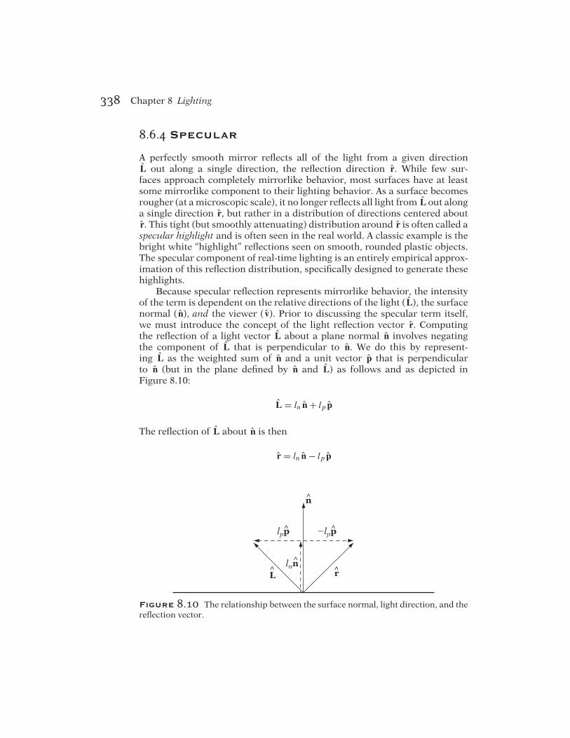
A perfectly smooth mirror reflects all of the light from a given directionL out along a single direction, the reflection direction r. While few sur-faces approach completely mirrorlike behavior, most surfaces have at leastsome mirrorlike component to their lighting behavior. As a surface becomesrougher (at amicroscopic scale), it no longer reflects all light from L out alonga single direction r, but rather in a distribution of directions centered aboutr. This tight (but smoothly attenuating) distribution around r is often called aspecular highlight and is often seen in the real world. A classic example is thebright white “highlight” reflections seen on smooth, rounded plastic objects.The specular component of real-time lighting is an entirely empirical approx-imation of this reflection distribution, specifically designed to generate thesehighlights.

Because specular reflection represents mirrorlike behavior, the intensityof the term is dependent on the relative directions of the light (L), the surfacenormal ( n), and the viewer ( v). Prior to discussing the specular term itself,we must introduce the concept of the light reflection vector r. Computingthe reflection of a light vector L about a plane normal n involves negatingthe component of L that is perpendicular to n. We do this by represent-ing L as the weighted sum of n and a unit vector p that is perpendicularto n (but in the plane defined by n and L) as follows and as depicted inFigure 8.10:

L = ln n+ lp p

The reflection of L about n is then

r = ln n− lp p

lnnr

n

^ ^lpp lpp

L^

Figure 8.10 The relationship between the surface normal, light direction, and thereflection vector.


We know that the component of L in the direction of n (ln) is the projectionof L onto n, or

ln = L · n

Now we can compute lp p by substitution of our value for ln:

L = ln n+ lp p

L = ( L · n) n+ lp p

lp p = L− ( L · n) n

So, the reflection vector r equals

r = ln n− lp p

= ( L · n) n− lp p

= ( L · n) n− ( L− ( L · n) n)

= ( L · n) n− L+ ( L · n) n

= 2( L · n) n− L

Computing the view vector involves having access to the camera location,so we can compute the normalized vector from the current sample locationto the camera center. In an earlier section, camera (or “eye”) space was men-tioned as a common space in which we could compute our lighting. If weassume that the surface sample location is in camera space, this simplifiesthe process, because the center of the camera is the origin of view space.Thus, the view vector is then the origin minus the surface sample location;that is, the zero vector minus the sample location. Thus, in camera space, theview vector is simply the negative of the sample position treated as a vectorand normalized.

The specular term itself is designed specifically to create an intensity dis-tribution that reaches its maximum when the view vector v is equal to r;that is, when the viewer is looking directly at the reflection of the light vector.The intensity distribution falls off toward zero rapidly as the angle between thetwo vectors increases, with a “shininess” control that adjusts how rapidly theintensity attenuates. The term is based on the following formula:

( r · v)mshine = (cos θ)mshine

where θ is the angle between r and v. The shininess factor mshine controls thesize of the highlight; a smaller value of mshine leads to a larger, more diffuse


highlight, which makes the surface appear more dull and matte, whereas alarger value of mshine leads to a smaller, more intense highlight, which makesthe surface appear shiny. This shininess factor is considered a property of thesurface material and represents how smooth the surface appears. Generally,the complete specular term includes a specular color defined on the material(MS), which allows the highlights to be tinted a given color. The specularlight color is often set to the diffuse color of the light, since a colored lightgenerally creates a colored highlight. In practice, however, the specular colorof the material is more flexible. Plastic and clear-coated surfaces (such asthose covered with clear varnish), whatever their diffuse color, tend to havewhite highlights, while metallic surfaces tend to have tinted highlights. For amore detailed discussion of this and several other (more advanced) specularreflection methods, see Chapter 16 of Foley et al. [38].

A visual example of a sphere lit from a single light source providing onlyspecular light is shown in Figure 8.11. The complete specular lighting term is

CS =

{

iLmax(0, ( r · v))mshineLSMS, if L · n > 0

0, otherwise

Note that, as with the diffuse term, a self-shadowing conditional is applied,(L · n > 0). However, unlike the diffuse case, we must make this term explicit,as the specular term is not directly dependent upon L · n. Simply clamping thespecular term to be greater than 0 could allow objects whose normals pointaway from the light to generate highlights, which is not correct. In otherwords, it is possible for r · v > 0, even if L · n < 0.

In our pipeline, both materials and lights have specular components butonly materials have specular exponents, as the specular exponent representsthe shininess of a particular surface. We will store the specular color of anobject’s material in the 3-vector shader uniform value materialSpecularColor.The specular exponent material property is the scalar shader uniform materi-alSpecularExp. As previously noted for ambient and diffuse lighting, we willcompute the specular component of a light by multiplying a scalar ambientlight factor, lightAmbDiffSpec.z, times the light color, giving (lightColor *lightAmbDiffSpec.z).

The shader code to compute the specular component is as follows:

// GLSL Codeuniform vec3 materialSpecularColor;uniform float materialSpecularExp;uniform vec3 lightAmbDiffSpec;uniform vec3 lightColor;

vec3 computeSpecularComponent(in vec3 surfaceNormal,


in vec4 surfacePosition,

in lightSampleValues light)

{

vec3 viewVector = normalize(-surfacePosition.xyz);

vec3 reflectionVector

= 2.0 * dot(light.L, surfaceNormal) * surfaceNormal

- light.L;

return (dot(surfaceNormal, light.L) <= 0.0)

? vec3(0.0,0.0,0.0)

: (light.iL * (lightColor * lightAmbDiffSpec.z)

* materialSpecularColor

* pow(max(0.0, dot(reflectionVector, viewVector)),

materialSpecularExp));

}

Figure 8.11 Sphere lit by specular light.


Infinite Viewer Approximation

One of the primary reasons that the specular term is the most expensivecomponent of lighting is the fact that a normalized view and reflection vectormust be computed for each sample, requiring at least one normalization persample, per light. However, there is another method of approximating spec-ular reflection that can avoid this expense in common cases. This method isbased on a slightly different approximation to the specular highlight geome-try, along with an assumption that the viewer is “at infinity” (at least for thepurposes of specular lighting).

Rather than computing rdirectly, theOpenGLmethoduseswhat is knownas a halfway vector. The halfway vector is the vector that is the normalizedsum of L and v:

h =L + v

|L + v|

The resulting vector bisects the angle between L and v. This halfway vectoris equivalent to the surface normal n that would generate r such that r = v.In other words, given fixed light and view directions, h is the surface nor-mal that would produce the maximum specular intensity. So, the highlight isbrightest when n = h. Figure 8.12 is a visual representation of the configura-tion, including the surface orientation of maximum specular reflection. Theresulting (modified) specular term is

CS =

{

iLmax(0, ( h · n))mshineLSMS, if L · n > 0

0, otherwise

v

h^

^

Surface orientation resultingin maximum specularreflection (defined by h)

L^

Figure 8.12 The specular halfway vector.

8.7 Combined Lighting Equation 343

By itself, this new method of computing the specular highlight wouldnot appear to be any better than the reflection vector system. However, if weassume that the viewer is at infinity, then we can use a constant view vectorfor all vertices, generally the camera’s view direction. This is analogous to thedifference between a point light and a directional (infinite) light. Thanks tothe fact that the halfway vector is based only on the view vector and the lightvector, the infinite viewer assumption can reap great benefits when used withdirectional lights. Note that in this case, both L and v are constant across allsamples, meaning that the halfway vector h is also constant. Used together,these facts mean that specular lighting can be computed very quickly if direc-tional lights are used exclusively and the infinite viewer assumption is enabled.The halfway vector then can be computed once per object and passed downas a shader uniform, as follows:

// GLSL Codeuniform vec3 materialSpecularColor;uniform float materialSpecularExp;uniform vec3 lightAmbDiffSpec;uniform vec3 lightColor;uniform vec3 lightHalfway;

vec3 computeSpecularComponent(in vec3 surfaceNormal,in lightSampleValues light)

{return (dot(surfaceNormal, light.L) <= 0.0)

? vec3(0.0,0.0,0.0): (light.iL * (lightColor * lightAmbDiffSpec.z)

* materialSpecularColor* pow(max(0.0, dot(surfaceNormal, lightHalfway)),

materialSpecularExp));}

8.7 Combined Lighting Equation

Having covered materials, lighting components, and light sources, we nowhave enough information to evaluate our full lighting model for a given lightat a given point.

CV = Emissive

+(

Ambient+Diffuse+ Specular)

= ME + (CA + CD + CS)

AV = MAlpha

(8.1)


where the results are

1. CV , the computed, lit RGB color of the sample.

2. AV , the alpha component of the RGBA color of the sample.

The intermediate, per-light values used to compute the results are

3. CA, the ambient light term, which is equal to

CA = iLMALA

4. CD, the diffuse light term, which is equal to

CD = iLMDLD(max(0, L · n))

5. CS , the specular light term, which is equal to

CS = iLMSLS

{

max(0, ( h · n))mshine , if L · n > 0

0, otherwise

The shader code to compute this, based upon the shader functions alreadydefined previously, is as follows:

// GLSL Code

vec3 computeLitColor(in lightSampleValues light,in vec4 surfacePosition,in vec3 surfaceNormal)

{return computeAmbientComponent(light)

+ computeDiffuseComponent(surfaceNormal, light)+ computeSpecularComponent(surfaceNormal,

surfacePositon,light);

}

// ...

uniform vec3 materialEmissiveColor;uniform vec4 materialDiffuseColor;

vec4 finalColor;finalColor.rgb = materialEmissiveColor

+ computeLitColor(light, pos, normal);finalColor.a = materialDiffuseColor.a;


For a visual example of all of these components combined, see the litsphere in Figure 8.13.

Source Code

Demo

MultipleLights

Most interesting scenes will containmore than a single light source. Thus,the lighting model and the code must take this into account. When lightinga given point, the contributions from each component of each active light Lare summed to form the final lighting equation, which is detailed as follows:

CV = Emissive+ Ambient

+

lights∑

L

(

Per-light Ambient+ Per-light Diffuse+ Per-light Specular)

= ME +

lights∑

L

(CA + CD + CS) (8.2)

AV = MAlpha

The combined lighting equation 8.2 brings together all of the propertiesdiscussed in the previous sections. In order to implement this equation in

Figure 8.13 Sphere lit by a combination of ambient, diffuse, and specular lighting.


shader code, we need to compute iL and L per active light. The shader codefor computing these values required source data for each light. In addition, thetype of data required differed by light type. The former issue can be solvedby passing arrays of uniforms for each value required by a light type. Theelements of the arrays represent the values for each light, indexed by a loopvariable. For example, if we assume that all of our lights are directional, thecode to compute the lighting for up to eight lights might be as follows:

// GLSL Codeuniform vec3 materialEmissiveColor;uniform vec3 materialAmbientColor;uniform vec4 materialDiffuseColor;uniform vec3 materialSpecularColor;uniform float materialSpecularExp;uniform int dirLightCount;uniform vec4 dirLightPosition[8];uniform float dirLightIntensity[8];uniform vec3 lightAmbDiffSpec[8];uniform vec3 lightColor[8];

lightSampleValues computeDirLightValues(in int i){

lightSampleValues values;values.L = dirLightPosition[i];values.iL = dirLightIntensity[i];return values;

}

vec3 computeAmbientComponent(in lightSampleValues light,in int i)

{return light.iL * (lightColor[i] * lightAmbDiffSpec[i].x)

* materialAmbientColor;}

vec3 computeDiffuseComponent(in vec3 surfaceNormal,in lightSampleValues light,in int i)

{return light.iL * (lightColor[i] * lightAmbDiffSpec[i].y)

* materialDiffuseColor.rgb* max(0.0, dot(surfaceNormal, light.L));

}

vec3 computeSpecularComponent(in vec3 surfaceNormal,


in vec4 surfacePositon,in lightSampleValues light,in int i)

{vec3 viewVector = normalize(-surfacePosition.xyz);vec3 reflectionVector

= 2.0 * dot(light.L, surfaceNormal) * surfaceNormal- light.L;

return (dot(surfaceNormal, light.L) <= 0.0)? vec3(0.0,0.0,0.0): (light.iL * (lightColor[i] * lightAmbDiffSpec[i].z)

* materialSpecularColor* pow(max(0.0, dot(reflectionVector, viewVector)),

materialSpecularExp));}

vec3 computeLitColor(in lightSampleValues light,in vec4 surfacePosition,in vec3 surfaceNormal, in int i)

{return computeAmbientComponent(light, i)

+ computeDiffuseComponent(surfaceNormal, light, i)+ computeSpecularComponent(surfaceNormal,

surfacePositon,light, i);

}

{int i;vec4 finalColor;finalColor.rgb = materialEmissiveColor;finalColor.a = materialDiffuseColor.a;for (i = 0; i < dirLightCount; i++){

lightSampleValues light = computeDirLightValues(i);finalColor.rgb + =

computeLitColor(light, i, pos, normal);}

}

The code becomes even more complex when we must consider differenttypes of light sources. One approach to this is to use independent arrays foreach type of light and iterate over each array independently. The complexity of


these approaches and the number of uniforms that must be sent to the shadercan be prohibitive for some systems. As a result, it is common for renderingengines to either generate specific shaders for the lighting cases they knowthey need, or else generate custom shader source code in the engine itself,compiling these shaders at runtime as they are required.

Clearly, many different values and components must come together tolight even a single sample. This fact can make lighting complicated and dif-ficult to use at first. A completely black rendered image or a flat-coloredresulting object can be the result of many possible errors. However, an under-standing of the lighting pipeline can make it much easier to determine whichfeatures to disable or change in order to debug lighting issues.

8.8 Lighting and Shading

Thus far, our lighting discussion has focused on computing color at a genericpoint on a surface, given a location, surface normal, view vector, and surfacematerial. We have specifically avoided specifying whether these code snippetsin our shader code examples are to be vertex or fragment shaders. Anotheraspect of lighting that is just as important as the basic lighting equation isthe question of when and how to evaluate that equation to completely light asurface. Furthermore, if we do not choose to evaluate the full lighting equa-tion at every sample point on the surface, how do we interpolate or reusethe explicitly lit sample points to compute reasonable colors for these othersamples.

Ultimately, a triangle in view is drawn to the screen by coloring the screenpixels covered by that triangle (as will be discussed in more detail in Chap-ter 9). Any lighting system must be teamed with a shading method that canquickly compute colors for each and every pixel covered by the triangle. Theseshading methods determine when to invoke the shader to compute the light-ing and when to simply reuse or interpolate already computed lighting resultsfrom other samples. In most cases, this is a performance versus visual accu-racy trade-off, since it is normallymore expensive computationally to evaluatethe shader than it is to reuse or interpolate already computed lighting results.

The sheer number of pixels that must be drawn per frame requires thatlow- to mid-end graphics systems forego computing more expensive lightingequations for each pixel in favor of another method. For example, a spherethat covers 50 percent of a mid-sized 1,280 × 1,024 pixel screen will requirethe shading system to compute colors for over a half million pixels, regardlessof the tessellation. Next, we will discuss some of the more popular methods.Some of these methods will be familiar, as they are simply the shading meth-ods discussed in Chapter 7, using results of the lighting equation as sourcecolors.

8.8 Lighting and Shading 349

8.8.1 Flat-Shaded Lighting

Historically, the simplest shadingmethod applied to lighting was per-triangle,flat shading. This method involved evaluating the lighting equation once pertriangle and using the resulting color as the constant triangle color. This coloris assigned to every pixel covered by the triangle. In older, fixed-function sys-tems, this was the highest-performance lighting/shading combination, owingto two facts: themore expensive lighting equation needed only to be evaluatedonce per triangle, and a single color could be used for all pixels in the triangle.Figure 8.14 shows an example of a sphere lit and shaded using per-trianglelighting and flat shading.

To evaluate the lighting equation for a triangle, we need a sample locationand surface normal. The surface normal used is generally the triangle facenormal (discussed in Chapter 2), as it accurately represents the plane of thetriangle. However, the issue of sample position ismore problematic. No singlepoint can accurately represent the lighting across an entire triangle (except inspecial cases); for example, in the presence of a point light, different pointson the triangle should be attenuated differently, according to their distance

Figure 8.14 Sphere lit and shaded by per-triangle lighting and flat shading.


from the light. While the centroid of the triangle is a reasonable choice, thefact that it must be computed specifically for lighting makes it less desirable.For reasons of efficiency (and often to match with the graphics system), themost common sample point for flat shading is one of the triangle vertices, asthe vertices already exist in the desired space. This can lead to artifacts, sincea triangle’s vertices are (by definition) at the edge of the area of the triangle.Flat-shaded lighting does notmatch quite as well withmodern programmableshading pipelines, and the simplicity of the resulting lighting has meant thatit is of somewhat limited interest in modern rendering systems.

8.8.2 Per-Vertex Lighting

Flat-shaded lighting suffers from the basic flaws and limitations of flat shadingitself; the faceted appearance of the resulting geometry tends to highlightrather than hide the piecewise triangular approximation. In the presence ofspecular lighting, the tessellation is even more pronounced, causing entiretriangles to be lit with bright highlights. With moving lights or geometry, thiscan cause gemstonelike “flashing” of the facets. For smooth surfaces such asthe sphere in Figure 8.14 this faceting is often unacceptable.

The next logical step is to use per-vertex lighting with Gouraud interpo-lation of the resulting color values. The lighting equation is evaluated in thevertex shader, and the resulting color is passed as an interpolated varyingcolor to the simple fragment shader. The fragment shader can be extremelysimple, doing nothing more than assigning the interpolated varying color asthe final fragment color.

Generating a single lit color that is shared by all colocated vertices leads tosmooth lighting across surface boundaries. Even if colocated vertices are notshared (i.e., each triangle has its own copy of its three vertices), simply settingthe normals to be the same in all copies of a vertex will cause all copies tobe lit the same way. Figure 8.15 shows an example of a sphere lit and shadedusing per-vertex lighting and Gouraud shading.

Per-vertex lighting only requires evaluating the lighting equation once pervertex. In the presence of well-optimized vertex sharing (where there aremoretriangles than vertices), per-vertex lighting can actually require fewer lightingequation evaluations than does true per-triangle flat shading. The interpola-tion method used to compute the per-fragment varying values (Gouraud) ismore expensive computationally than the trivial one used for flat shading,since it must interpolate between the three vertex colors on a per-pixel basis.However, modern shading hardware is heavily tuned for this form of vary-ing value interpolation, so the resulting performance of per-vertex lighting isgenerally close to peak.

Gouraud-shaded lighting is a vertex-centric method—the surface posi-tions and normals are used only at the vertices, with the triangles serving


Figure 8.15 Sphere lit and shaded by per-vertex lighting and Gouraud shading.

only as areas for interpolation. This shift to vertices as localized surfacerepresentations lends focus to the fact that we will need smooth surfacenormals at each vertex. The next section will discuss several methods forgenerating these vertex normals.

Generating Vertex Normals

In order to generate smooth lighting that represents a surface at each vertex,we need to generate a single normal that represents the surface at each vertex,not at each triangle. There are several commonmethods used to generate theseper-vertex surface normals at content creation time or at load time, dependingupon the source of the geometry data.

When possible, the best way to generate smooth normals during the cre-ation of a tessellation is to use analytically computed normals based on thesurface being approximated by triangles. For example, if the set of trianglesrepresent a sphere centered at the origin, then for any vertex at location PV ,the surface normal is simply

n =PV − 0

|PV − 0|


This is the vertex position, treated as a vector (thus the subtraction ofthe zero point) and normalized. Analytical normals can create very realisticimpressions of the original surface, as the surface normals are pivotal tothe overall lighting impression. Examples of surfaces for which analyti-cal normals are available include implicit surfaces and parametric surfacerepresentations, which generally include analytically defined normal vectorsat every point in their domain.

In the more common case, the mesh of triangles exists by itself, with noavailable method of computing exact surface normals for the surface beingapproximated. In this case, the normals must be generated from the trian-gles themselves. While this is unlikely to produce optimal results in all cases,simple methods can generate normals that tend to create the impression of asmooth surface and remove the appearance of faceting.

One of themost popular algorithms for generating normals from trianglestakes the mean of all of the face normals for the triangles that use the givenvertex. Figure 8.16 demonstrates a two-dimensional (2D) example of averag-ing triangle normal vectors. The algorithm may be pseudo-coded as follows:

for each vertex V{

vector V.N = (0,0,0);for each triangle T that uses V{

vector F = TriangleNormal(T);V.N += F;

} V.N.Normalize();}

Triangles (side view)

True triangle normals Averaged vertex normals

Figure 8.16 Averaging triangle normal vectors.


Basically, the algorithm sums the normals of all of the faces that areincident upon the current vertex and then renormalizes the resulting summedvector. Since this algorithm is (in a sense) a mean-based algorithm, it can beaffected by tessellation. Triangles are not weighted by area or other such fac-tors, meaning that the face normal of each triangle incident upon the vertexhas an equal “vote” in themakeup of the final vertex normal.While themethodis far from perfect, any vertex normal generated from triangles will by itsnature be an approximation. Inmost cases, the averaging algorithm generatesconvincing normals. Note that in cases where there is no fast (i.e., constant-time) method of retrieving the set of triangles that use a given vertex (e.g., ifonly the OpenGL/Direct3D-style index lists are available), the algorithm maybe turned “inside out” as follows:

for each vertex V{

V.N = (0,0,0);}for each triangle T{

// V1, V2, V3 are the vertices used by the trianglevector F = TriangleNormal(T);V1.N += F;V2.N += F;V3.N += F;

}for each vertex V{

V.N.Normalize();}

Basically, this version of the algorithm uses the vertex normals as “accumu-lators,” looping over the triangles, adding each triangle’s face normal to thevertex normals of the three vertices in that triangle. Finally, having accumu-lated the input fromall triangles, the algorithmgoes back and normalizes eachfinal vertex normal. Both algorithmswill result in the same vertex normals, buteach works well with different vertex/triangle data structure organizations.

Sharp Edges

AswithGouraud shading based on fixed colors, Gouraud-shaded lightingwithvertices shared between triangles generates smooth triangle boundaries bydefault. In order to represent a sharp edge, vertices along a physical crease inthe geometry must be duplicated so that the vertices can represent the surface


normals on either side of the crease. By having different surface normals incopies of colocated vertices, the triangles on either side of an edge can be litaccording to the correct local surface orientation. For example, at each vertexof a cube, there will be three vertices, each one with a normal of a differentface orientation, as we see in Figure 8.17.

8.8.3 Per-Fragment Lighting

Source Code

Demo

PerFragmentLighting

There are significant limitations to per-vertex lighting. Specifically, the factthat the lighting equation is evaluated only at the vertices can lead to artifacts.Even a cursory evaluation of the lighting equation shows that it is highly non-linear. However, Gouraud shading interpolates linearly across polygons. Anynonlinearities in the lighting across the interior of the trianglewill be lost com-pletely. These artifacts are not as noticeable with diffuse and ambient lightingas they are with specular lighting, because diffuse and ambient lighting arecloser to linear functions than is specular lighting (owing at least partially to

V1

V2

V3

Figure 8.17 One corner of a faceted cube.


the nonlinearity of the specular exponent term and to the rapid changes inthe specular halfway vector h with changes in viewer location).

For example, let us examine the specular lighting term for the sur-face shown in Figure 8.18. We draw the 2D case, in which the triangle isrepresented by a line segment. In this situation, the vertex normals all pointoutward from the center of the triangle, meaning that the triangle is repre-senting a somewhat curved (domed) surface. The point light source and theviewer are located at the same position in space, meaning that the view vec-tor v, the light vector L, and the resulting halfway vector hwill all be equal forall points in space. The light and viewer are directly above the center of the tri-angle. Because of this, the specular components computed at the two verticeswill be quite dark (note the specular halfway vectors shown in Figure 8.18 arealmost perpendicular to the normals at the vertices). Linearly interpolatingbetween these two dark specular vertex colors will result in a polygon that isrelatively dark.

However, if we look at the geometry that is being approximated by thesenormals (a domed surface as in Figure 8.18), we can see that in this configura-tion the interpolated normal at the center of the triangle would point straightup at the viewer and light. If we were to evaluate the lighting equation at a

Gouraud shadingof single triangle

Correct lighting ofsmooth surface

Approximated(smooth) surface

Viewer Point light

n • h ≈ 0^ ^n • h ≈ 0^ ^

nn

L v h^ ^ ^

L v h^ ^ ^

Figure 8.18 Gouraud shading can miss specular highlights.


Phong shading ofsingle triangle

Correct lighting ofsmooth surface

n • h ≈ 0^ ^n • h ≈ 0^ ^

nn

Interpolatedvertex normal

n • h ≈ 1^ ^

v h L n^ ^^ ^

Viewer Point light

Figure 8.19 Phong shading of the same configuration.

point near the center of the triangle in this case, we would find an extremelybright specular highlight there. The specular lighting across the surface ofthis triangle is highly nonlinear, and the maximum is internal to the trian-gle. Even more problematic is the case in which the surface is moving overtime. In rendered images where the highlight happens to line up with a vertex,there will be a bright, linearly interpolated highlight at the vertex. However,as the surface moves so that the highlight falls between vertices, the high-light will disappear completely. This is a very fundamental problem withapproximating a complex functionwith a piecewise linear representation. Theaccuracy of the result is dependent upon the number of linear segments usedto approximate the function. In our case, this is equivalent to the density of thetessellation.

If we want to increase the accuracy of lighting on a general vertex-litsurface, we must subdivide the surface to increase the density of vertices(and thus lighting samples). However, this is an expensive process, and wemay not know a priori which sections of the surface will require significanttessellation. Dependent upon the particular view at runtime, almost any tes-sellation may be either overly dense or too coarse. In order to create a moregeneral, high-quality lighting method, we must find another way around thisproblem.

So far, the methods we have discussed for lighting have all evaluated thelighting equation once per basic geometric object, such as per vertex or pertriangle. Phong shading (named after its inventor, Bui Phong Tuong [93])


works by evaluating the lighting equation once for each fragment covered bythe triangle. The difference betweenGouraud and Phong shadingmay be seenin Figures 8.18 and 8.19. For each sample across the surface of a triangle, thevertex normals, positions, reflection, and view vectors are interpolated, andthe interpolated values are used to evaluate the lighting equation. However,since triangles tend to cover more than 1–3 pixels, such a lighting method willresult in far more lighting computations per triangle than do per-triangle orper-vertex methods.

Per-fragment lighting changes the balance of the work to be done in thevertex and fragment shaders. Instead of computing the lighting in the vertexshader, per-pixel lighting uses the vertex shader only to set up the source val-ues (surface position, surface normal, view vector) and pass them down asvarying values to the fragment shader. As always, the varying values are inter-polated using Gouraud interpolation and passed to each invocation of thefragment shaders. These interpolated values now represent smoothly inter-polated position and normal vectors for the surface being represented. It isthese values that are used as sources to the lighting computations, evaluatedin the fragment shader.

There are several issues that make Phong shading more computationallyexpensive than per-vertex lighting. The first of these is the actual normal vectorinterpolation, since basic barycentric interpolation of the three vertex normalswill almost never result in a normalized vector. As a result, the interpolatednormal vector will have to be renormalized per fragment, which is much morefrequently than per vertex.

Furthermore, the full lighting equation must be evaluated per sampleonce the interpolated normal is computed and renormalized. Not onlyis this operation expensive, it is not a fixed amount of computation. Aswe saw above, in a general engine, the complexity of the lighting equa-tion is dependent on the number of lights and numerous graphics enginesettings. This resulted in Phong shading being rather unpopular in game-centric consumer 3D hardware prior to the advent of pixel and vertexshaders.

An example of a vertex shader passing down the required camera-spacepositions and normals is as follows:

// GLSLvarying vec4 lightingPosition;varying vec3 lightingNormal;

void main(){

// The position and normal for lighting// must be in camera space, not homogeneous spacelightingPosition = gl_ModelViewMatrix * gl_Vertex;


lightingNormal = gl_NormalMatrix * gl_Normal;

gl_Position = gl_ModelViewProjectionMatrix * gl_Vertex;}

An example of a fragment shader implementing lighting by a singledirectional light is as follows:

// GLSL Codeuniform vec3 materialEmissiveColor;uniform vec3 materialAmbientColor;uniform vec4 materialDiffuseColor;uniform vec3 materialSpecularColor;uniform vec4 dirLightPosition;uniform float dirLightIntensity;uniform vec3 lightAmbDiffSpec;uniform vec3 lightColor;

varying vec4 lightingPosition;varying vec3 lightingNormal;

{vec4 finalColor;finalColor.rgb = materialEmissiveColor;finalColor.a = materialDiffuseColor.a;

vec3 interpolatedNormal = normalize(lightingNormal);

lightSampleValues light = computeDirLightValues();finalColor.rgb += computeLitColor(light,

lightingPosition, interpolatedNormal);}

}

8.9 Textures and Lighting

Source Code

Demo

TexturesAndLighting

Of the methods we have discussed for coloring geometry, the two most pow-erful are texturing and dynamic lighting. However, they each have drawbackswhen used by themselves. Texturing is normally a static method and looksflat and painted when used by itself in a dynamic scene. Lighting can gener-ate very dynamic effects, but when limited to per-face-level or per-vertex-levelfeatures, can lead to limited detail. It is only natural that graphics systemswould want to use the results of both techniques together on a single surface.

8.9 Textures and Lighting 359

8.9.1 Basic Modulation

The simplest methods of merging these two techniques involves simplyviewing each of the twomethods as generating a color per sample andmergingthem. With texturing, this is done directly via texture sampling; with lighting,it is done by evaluating the lighting equation. These two colors must be com-bined in a way that makes visual sense. The most common way of combiningtextures and lighting results is via multiplication, or “modulation.” In modu-late lighting/texture combination, the texture color at the given sampleCT andthe final lit and/or interpolated vertex color are combined by per-componentmultiplication.

The visual effect here is that the per-vertex lit colors darken the texture(or vice versa). As a result, texture images designed to be used with modu-late mode texture combination are normally painted as if they were fully lit.The vertex colors, representing the lighting in the scene, darken these fullylit textures to make them look more realistic in the given environment. AsFigure 8.20 demonstrates, the result of modulation can be very convincing,even though the lighting is rather simple and the textures are static paintings.In the presence of moving or otherwise animated lights, the result can be evenmore immersive, as the human perceptual system is very reliant upon lightingcues in the real world. This is, in a sense, using the texture as a factor in allof the surface material colors.

(a)

(b)

(c)

Figure 8.20 Textures and lighting combined via modulation: (a) scene with purevertex lighting, (b) scene with pure texturing, and (c) same scene with lighting andtexturing combined.


Assuming for the moment that the lit color is computed and stored inlitColor, either by computation in the fragment shader or passed down asa varying component, a simple textured, lit fragment shader would be asfollows:

// GLSL - fragment shaderuniform sampler2D texture;varying vec2 texCoords;

void main(){

// lit color is in vec4 litColorvec4 litColor;

// ...

// Sample the texture represented by "texture"// at the location "texCoords"gl_FragColor = litColor * texture2D (texture, texCoords);

}

Until the advent of programmable shaders, modulation was the mostpopular and often the only method of combining lighting and textures.

8.9.2 Specular Lighting and Textures

If the full lighting equation 8.1 is combined with the texture via multipli-cation, then lighting can only darken the texture, since lit vertex colors areclamped to the range [0, 1]. While this looks correct for diffuse or matteobjects, for shiny objects with bright specular highlights, it can look very dull.It is often useful to have the specular highlights “wash out” the texture. Wecannot simply add the full set of lighting because the texturewill almost alwayswash out and can never get darker. To be able to see the full range of effectsrequires that the diffuse colors darken the texture while the specular com-ponents of color add highlights. This is only possible if we split the lightingcomponents.

Because the specular term is added after the texture is multiplied, thismode (sometimes called modulate with late add) causes the diffuse terms toattenuate the texture color, while the specular terms wash out the result. Thedifferences between the separate and combined specular modes can be verystriking, as Figure 8.21 makes clear.

The shader code to compute this involves computing the emissive,ambient, and diffuse lighting components into one color (which we’ll call

8.9 Textures and Lighting 361

(a) (b)

Figure 8.21 Combining textures and lighting: (a) specular vertex color added todiffuse vertex color, then modulated with the texture, and (b) diffuse vertex colormodulated with the texture, then specular vertex color added.

diffuseLighting) and the specular component into another (which we’ll callspecularLighting). Having computed these independently, we merge them asfollows:


void main(){

vec4 diffuseLighting;vec4 specularLighting;

// ...

// Sample the texture represented by "texture"// at the location "texCoords"gl_FragColor = diffuseLighting * texture2D (texture, texCoords)

+ specularLighting;}

In this case, the texture is providing a scaling factor for only the emissive,ambient, and diffuse material color. The effect is simple to add to an exist-ing lighting and texture shader and can make for a much more dynamicresult.


8.9.3 Textures as Materials

The next step in using textures and lighting together involves using multipletextures on a single surface. As shown in the previous section, a texture canbe used to modulate one or more material colors on a surface. In fact, tex-tures also can be used to replace one or more surface material components.Common surface material colors to be replaced with textures are:

� Material diffuse color. Often called a diffuse map, this is extremelysimilar to basic modulation as shown above. Frequently, the diffusemap is also applied as the ambient material color.

� Material specular color. This is frequently replaced with either anRGB texture (a specular map) or a single-channel grayscale texture,which is called a gloss map. The gloss map is a powerful technique:Wherever it is close to full brightness, the object appears glossy,because specular highlights can be seen at those points on the surface.Wherever it is close to black, the specular highlights do not appear. Asa result, it can be used to mark shiny or worn sections of an object,independent of the color. Frequently, gloss maps are created in such away that they are brightest on the edges and exposed areas, parts of asurface likely to be worn down by the elements and naturally polished.

� Material emissive color. Often called a glow map, this texture canbe used to localize self-illumination of an object. These maps arefrequently used to mark windows in nighttime views of vehicles orbuildings, or taillights and running lights of vehicles.

Since multiple textures can be used in a single shader, any or all of thesecomponents can be easily replaced by individual textures. The uniformmate-rial color vectors simply become texture sampler uniforms. Many of thesetextures can reuse the same texture coordinates, as the mappings of each tex-ture can be the same. Finally, optimizations are common. For example, it iscommon to use an RGBA texture in which the RGB components are used asthe diffuse map, and the alpha component is used as a single-channel glossmap. The ease of painting these components into a single texture can assistthe artists, and the reuse of an otherwise unused texture component can savegraphics processing unit (GPU) resources. An example of a fragment shaderusing RGBA diffuse and gloss maps is shown below:


8.10 Advanced Lighting 363

void main(){

vec4 diffuseLighting;vec4 specularLighting;

// ...vec4 diffuseAndGlossMap = texture2D (texture, texCoords);

// Sample the texture represented by "texture"// at the location "texCoords"gl_FragColor.rgb = diffuseLighting.rgb * diffuseAndGlossMap.rgb

+ specularLighting.rgb * diffuseAndGlossMap.a;}

8.10 Advanced Lighting

Programmable shaders make an almost endless array of lighting effects possi-ble. We will discuss a few of these methods and mention several others, citingreferences for additional information. Like themethodsmentioned in the pre-vious sections, many of these methods involve using textures as sources to thelighting equation.

8.10.1 Normal Mapping

Source Code

Demo

NormalMapping

So far, we have shown how one or more textures can be used to replace mate-rial colors and/or intensities in the lighting equation. However, even moreadvanced techniques are based on the fact that textures can be used to storemore general values than mere colors. The most popular of these techniquesare bumpmapping and normal mapping. As the names suggest, these methodssimulate bumpy surfaces by storing the detailed “height offsets” (bump map-ping) or normal vectors (normal mapping) for the surface in a texture. Oneof the basic limitations of dynamic lighting as discussed so far is that whilewe can evaluate lighting on a per-fragment basis, the source values describ-ing the geometry of the surface are interpolated from per-vertex values— theposition and normal. As a result, a rough or bumpy surface requires a veryhigh density of vertices. We can simulate this effect at a finer level by addingbumpy, pre-lit colors to the diffuse map texture, but in the presence of mov-ing or changing lighting conditions, the static nature of this trick is obviousand jarring. Bump mapping, the first of these techniques to be available, wasactually present in some fixed-function rendering hardware in the late 1990s.However, bump mapping, since it represented a local height offset and gen-erated surface normals implicitly by looking at the difference in height values


between neighboring texels, was limited to surfaces that looked embossed.Very sharp changes in surface orientation were difficult with bump mapping.For a discussion of these limitations, see Theodore [110].

In order to add more detail to the lighting at this fine level, we must beable to generate a surface normal per fragment that contains real information(not just interpolated information) for each fragment. By storing the normalin a texture, we can generate normals that change very rapidly per fragmentand respond correctly to changing lighting configurations. The normal vectorsacross the surface are stored in the RGB components of the texture (eitheras signed fixed-point values or as floating-point values). The exact space inwhich the normals are stored in the texture differs from method to method.Conceptually, the simplest space is object space, in which normals are com-puted in the model or object space of the geometry being mapped and thenstored as (x,y,z) in the R, G, and B components of the texture, respectively.Object-space normal maps can be sampled as a regular texture into a vec3 andthen used in the same way as one would use normals passed into a fragmentshader as a varying value. An example of the effect that normal mapping canhave on a simple object is shown in Figure 8.22

An example of an object-space normal map in use in a fragment shader isshown below. Note that since the sampled normal comes from the texture inobject space, we must either do the transformation of the normal into cameraspace in the fragment shader, or else transform the light information intomodel space and light inmodel space.We pick the former (which is simpler to

(a) (b)

Figure 8.22 Normal mapping applied to simple objects: (a) low triangle—countobject with diffuse map and per-vertex lighting, and (b) same object with diffuse mapand per-fragment normal mapping.

8.10 Advanced Lighting 365

understand, but more expensive computationally) and transform the normalinto camera space.

// GLSL Codeuniform sampler2D normalMap; varying vec2 texCoords;uniform vec3 materialEmissiveColor;uniform vec3 materialAmbientColor;uniform vec4 materialDiffuseColor;uniform vec3 materialSpecularColor;uniform vec4 dirLightPosition;uniform float dirLightIntensity;uniform vec3 lightAmbDiffSpec;uniform vec3 lightColor;

varying vec4 lightingPosition;

{vec4 finalColor;finalColor.rgb = materialEmissiveColor;finalColor.a = materialDiffuseColor.a;

// lookup the normal in the map, transform, and renormalizevec3 normal = texture2D (normalMap, texCoords);normal = normalize(gl_NormalMatrix * normal);

lightSampleValues light = computeDirLightValues();finalColor.rgb += computeLitColor(light,

lightingPosition, normal);}

}

There are advantages anddisadvantages to both object-space normalmap-ping and the other common normal mappingmethod, known as tangent space

normal maps (the latter is now the more popular of the two, but is concep-tually a bit harder to understand). These differences are discussed in variousarticles on normal mapping [36, 92].

Generating Normal Maps

Normal maps are rarely painted by an artist. The complexity of these mapsand the esoteric spaces in which they reside mean that most normal mapsare generated automatically from the geometry itself via commercial or open-source tools. Some real-time 3D engines and middleware provide tools that


automatically convert a very high polygon–count object (millions of triangles)into a low polygon–count geometry object and a high-resolution normal map.Put together, the low-resolution geometry object and the high-resolution nor-malmap can be used to efficiently renderwhat appears to be a very convincingfacsimile of the original object.

8.11 Reflective Objects

While specular lighting can provide the basic impression of a shiny object,large expanses of a reflective surface are more convincing if they actuallyappear to reflect the other geometry in the scene. The best-known method forthis is the (generally) non-real-time method of recursive ray tracing, which isnot currently suitable for general interactive systems. However, we can onceagain use a mixture of lightinglike computations and textures to create veryconvincing reflections.

Environment mapping is a technique that uses a texture or set of texturesthat represents an “inside looking out” representation of the entire scene inall directions. It can be thought of as a spherical or cube-shaped set of imagesthat represent a panorama of the scene. These images can be statically drawnoffline, or on modern systems can even be rendered every frame to better rep-resent the current scene. The environment map can be thought of as infinitely

(a) (b)

Figure 8.23 Environment mapping applied to simple objects.

8.12 Shadows 367

large or infinitely distant. Thus, any normalized direction vector maps to asingle, fixed location in the environment map.

Environment maps are applied to a surface dynamically— they are notsampled via a priori texture coordinates; the mapping of the environmentmapwill change as the scene and the view changes. Themost commonmethodused is to compute the reflection of the view vector in amanner similar to thatused for specular lighting earlier in this chapter. The reflected view vector rep-resents the direction that the viewer sees in the reflective surface. By samplingthe environment map in this view direction, we can apply what appears to bea convincing reflection to a surface with little more than a vector computation(per vertex or per fragment) and a texture lookup (per fragment). Figure 8.23shows how this effect can be applied to a simple object. Note that in the twoviews of the object, the environment map moves like a reflection as the objectrotates with respect to the viewer.

8.12 Shadows

Shadows are an extremely important component of real-world lighting.However, while we think of them as a form of lighting, the challenge inrendering accurate shadows has little in common with the per-vertex andper-fragment direct lighting formulae we discussed earlier in this chapter.In a sense, shadowing is much less about lighting than it is about occlusionor intersection. Diffuse and specular lighting formulae are concerned mainlywith determining how the light incident upon a surface is reflected towardthe viewer. Shadowing, on the other hand, is far more concerned with deter-mining whether light from a given light source reaches the surface in the firstplace. Unlike surface lighting calculations, shadowing is dependent upon allof the objects that might interpose between the light source and the surfacebeing lit.

A single surface shader is rarely if ever enough to implement shadowing.Shadowing is generally a multipass technique over the entire scene. The firstpass involves determining which surfaces receive light from a given source,and the second pass involves applying this shadowing information to theshading of the objects in the scene. The many algorithms used to approxi-mate real-time shadows differ in their approaches to both passes. With theadvent of high-powered, programmable shading hardware, the push in shad-owing methods over the past decade has focused on leveraging the renderinghardware as much as possible for both passes, avoiding expensive CPU-basedcomputation. These algorithms have centered on the concept of using a firstpass that involves rendering the scene from the point of viewof the light source,as geometry visible from the point of view of the light is exactly the geometrythat will be lit by that light source. Geometry that cannot be “seen” from a


light’s location is exactly the geometry that will be in shadow. Geometry thatfalls on the boundaries of these two cases is likely to be in the penumbra, orpartially shadowed region, when rendering soft shadows.

Since the real core of shadowing methods lie in the structure of the two-pass algorithms rather than in the mathematics of lighting, the details ofshadowing algorithms are beyond the scope of this book. A technique knownas ray tracing (see Glassner [40]) uses ray–object intersection to track theway light bounces around a scene. Very convincing shadows (and reflections)could be computed using ray tracing, and the technique is very popular fornon-real-time rendering. Owing to its computational complexity, this methodis not generally used in real-time lighting (although modern shading lan-guages and shading hardware are now capable of doing real-time ray tracingin some limited cases). Shadows are sometimes approximated using othertricks (see [1, 83, 84], or Chapter 13 of Eberly [25]). Excellent references forreal-time shadows, both sharp and soft-edged, can be found in Fernando andPharr [36, 92].

8.13 Chapter Summary

In this chapter we have discussed the basics of dynamic lighting, both in termsof geometric concepts and implementation using programmable shaders. Per-vertex andper-pixel lighting are very powerful additions to any 3Dapplication,especiallywhenmatedwith the use ofmultiple textures. Correct use of lightingcan create compelling 3D environments at limited computational expense. Aswe have discussed, judicious use of lighting is important in order to maximizevisual impact while minimizing additional computation.

For further information, there are numerous paths available to the inter-ested reader. The growingwealth of shader resources includes websites [1, 84]and even book series [31]. Many of these new shaders are based on far moredetailed and complex lighting models, such as those presented in computergraphics conference papers and journal articles like those of ACMSIGGRAPHor in books such as Watt and Policarpo [117].

essential mathematics for games - cap 8 lighting.pdf

Documents