essentials of - dl.offdownload.ir of robust control.pdf · preface robustness of control systems to...
TRANSCRIPT


ESSENTIALS OFROBUST CONTROL
Kemin Zhou
May 25, 1999

Preface
Robustness of control systems to disturbances and uncertainties has always been thecentral issue in feedback control. Feedback would not be needed for most control systemsif there were no disturbances and uncertainties. Developing multivariable robust controlmethods has been the focal point in the last two decades in the control community. Thestate-of-the-art H∞ robust control theory is the result of this effort.
This book introduces some essentials of robust and H∞ control theory. It grew fromanother book by this author, John C. Doyle, and Keith Glover, entitled Robust andOptimal Control, which has been extensively class-tested in many universities aroundthe world. Unlike that book, which is intended primarily as a comprehensive reference ofrobust and H∞ control theory, this book is intended to be a text for a graduate coursein multivariable control. It is also intended to be a reference for practicing controlengineers who are interested in applying the state-of-the-art robust control techniquesin their applications. With this objective in mind, I have streamlined the presentation,added more than 50 illustrative examples, included many related Matlab
R commands1
and more than 150 exercise problems, and added some recent developments in the areaof robust control such as gap metric, ν-gap metric, model validation, and mixed µproblem. In addition, many proofs are completely rewritten and some advanced topicsare either deleted completely or do not get an in-depth treatment.
The prerequisite for reading this book is some basic knowledge of classical controltheory and state-space theory. The text contains more material than could be covered indetail in a one-semester or a one-quarter course. Chapter 1 gives a chapter-by-chaptersummary of the main results presented in the book, which could be used as a guide forthe selection of topics for a specific course. Chapters 2 and 3 can be used as a refresherfor some linear algebra facts and some standard linear system theory. A course focusingonH∞ control should cover at least most parts of Chapters 4–6, 8, 9, 11–13, and Sections14.1 and 14.2. An advanced H∞ control course should also include the rest of Chapter14, Chapter 16, and possibly Chapters 10, 7, and 15. A course focusing on robustnessand model uncertainty should cover at least Chapters 4, 5, and 8–10. Chapters 17 and18 can be added to any advanced robust and H∞ control course if time permits.
I have tried hard to eliminate obvious mistakes. It is, however, impossible for meto make the book perfect. Readers are encouraged to send corrections, comments, and
1Matlab is a registered trademark of The MathWorks, Inc.
vii

viii PREFACE
suggestions to me, preferably by electronic mail, [email protected]
I am also planning to put any corrections, modifications, and extensions on the Internetso that they can be obtained either from the following anonymous ftp:
ftp gate.ee.lsu.edu cd pub/kemin/books/essentials/or from the author’s home page:
http://kilo.ee.lsu.edu/kemin/books/essentials/This book would not be possible without the work done jointly for the previous
book with Professor John C. Doyle and Professor Keith Glover. I thank them for theirinfluence on my research and on this book. Their serious attitudes toward scientificresearch have been reference models for me. I am especially grateful to John for havingme as a research fellow in Caltech, where I had two very enjoyable years and hadopportunities to catch a glimpse of his “BIG PICTURE” of control.
I want to thank my editor from Prentice Hall, Tom Robbins, who originally proposedthe idea for this book and has been a constant source of support for me while writing it.Without his support and encouragement, this project would have been a difficult one.It has been my great pleasure to work with him.
I would like to express my sincere gratitude to Professor Bruce A. Francis for givingme many helpful comments and suggestions on this book. Professor Francis has alsokindly provided many exercises in the book. I am also grateful to Professor Kang-Zhi Liuand Professor Zheng-Hua Luo, who have made many useful comments and suggestions.I want to thank Professor Glen Vinnicombe for his generous help in the preparation ofChapters 16 and 17. Special thanks go to Professor Jianqing Mao for providing me theopportunity to present much of this material in a series of lectures at Beijing Universityof Aeronautics and Astronautics in the summer of 1996.
In addition, I would like to thank all those who have helped in many ways in makingthis book possible, especially Professor Pramod P. Khargonekar, Professor Andre Tits,Professor Andrew Packard, Professor Jie Chen, Professor Jakob Stoustrup, ProfessorHans Henrik Niemann, Professor Malcolm Smith, Professor Tryphon Georgiou, Profes-sor Tongwen Chen, Professor Hitay Ozbay, Professor Gary Balas, Professor CarolynBeck, Professor Dennis S. Bernstein, Professor Mohamed Darouach, Dr. Bobby Boden-heimer, Professor Guoxiang Gu, Dr. Weimin Lu, Dr. John Morris, Dr. Matt Newlin,Professor Li Qiu, Professor Hector P. Rotstein, Professor Andrew Teel, Professor Ja-gannathan Ramanujam, Dr. Linda G. Bushnell, Xiang Chen, Greg Salomon, Pablo A.Parrilo, and many other people.
I would also like to thank the following agencies for supporting my research: NationalScience Foundation, Army Research Office (ARO), Air Force of Scientific Research, andthe Board of Regents in the State of Louisiana.
Finally, I would like to thank my wife, Jing, and my son, Eric, for their generoussupport, understanding, and patience during the writing of this book.
Kemin Zhou

PREFACE ix
Here is how H∞ is pronounced in Chinese:
It means “The joy of love is endless.”


Contents
Preface vii
Notation and Symbols xv
List of Acronyms xvii
1 Introduction 11.1 What Is This Book About? . . . . . . . . . . . . . . . . . . . . . . . . . 11.2 Highlights of This Book . . . . . . . . . . . . . . . . . . . . . . . . . . . 31.3 Notes and References . . . . . . . . . . . . . . . . . . . . . . . . . . . . . 91.4 Problems . . . . . . . . . . . . . . . . . . . . . . . . . . . . . . . . . . . 10
2 Linear Algebra 112.1 Linear Subspaces . . . . . . . . . . . . . . . . . . . . . . . . . . . . . . . 112.2 Eigenvalues and Eigenvectors . . . . . . . . . . . . . . . . . . . . . . . . 122.3 Matrix Inversion Formulas . . . . . . . . . . . . . . . . . . . . . . . . . . 132.4 Invariant Subspaces . . . . . . . . . . . . . . . . . . . . . . . . . . . . . 152.5 Vector Norms and Matrix Norms . . . . . . . . . . . . . . . . . . . . . . 162.6 Singular Value Decomposition . . . . . . . . . . . . . . . . . . . . . . . . 192.7 Semidefinite Matrices . . . . . . . . . . . . . . . . . . . . . . . . . . . . 232.8 Notes and References . . . . . . . . . . . . . . . . . . . . . . . . . . . . . 242.9 Problems . . . . . . . . . . . . . . . . . . . . . . . . . . . . . . . . . . . 24
3 Linear Systems 273.1 Descriptions of Linear Dynamical Systems . . . . . . . . . . . . . . . . . 273.2 Controllability and Observability . . . . . . . . . . . . . . . . . . . . . . 283.3 Observers and Observer-Based Controllers . . . . . . . . . . . . . . . . . 313.4 Operations on Systems . . . . . . . . . . . . . . . . . . . . . . . . . . . . 343.5 State-Space Realizations for Transfer Matrices . . . . . . . . . . . . . . 353.6 Multivariable System Poles and Zeros . . . . . . . . . . . . . . . . . . . 383.7 Notes and References . . . . . . . . . . . . . . . . . . . . . . . . . . . . . 413.8 Problems . . . . . . . . . . . . . . . . . . . . . . . . . . . . . . . . . . . 42
xi

xii CONTENTS
4 H2 and H∞ Spaces 454.1 Hilbert Spaces . . . . . . . . . . . . . . . . . . . . . . . . . . . . . . . . 454.2 H2 and H∞ Spaces . . . . . . . . . . . . . . . . . . . . . . . . . . . . . . 474.3 Computing L2 and H2 Norms . . . . . . . . . . . . . . . . . . . . . . . . 534.4 Computing L∞ and H∞ Norms . . . . . . . . . . . . . . . . . . . . . . . 554.5 Notes and References . . . . . . . . . . . . . . . . . . . . . . . . . . . . . 614.6 Problems . . . . . . . . . . . . . . . . . . . . . . . . . . . . . . . . . . . 62
5 Internal Stability 655.1 Feedback Structure . . . . . . . . . . . . . . . . . . . . . . . . . . . . . . 655.2 Well-Posedness of Feedback Loop . . . . . . . . . . . . . . . . . . . . . . 665.3 Internal Stability . . . . . . . . . . . . . . . . . . . . . . . . . . . . . . . 685.4 Coprime Factorization over RH∞ . . . . . . . . . . . . . . . . . . . . . . 715.5 Notes and References . . . . . . . . . . . . . . . . . . . . . . . . . . . . . 775.6 Problems . . . . . . . . . . . . . . . . . . . . . . . . . . . . . . . . . . . 77
6 Performance Specifications and Limitations 816.1 Feedback Properties . . . . . . . . . . . . . . . . . . . . . . . . . . . . . 816.2 Weighted H2 and H∞ Performance . . . . . . . . . . . . . . . . . . . . . 856.3 Selection of Weighting Functions . . . . . . . . . . . . . . . . . . . . . . 896.4 Bode’s Gain and Phase Relation . . . . . . . . . . . . . . . . . . . . . . 946.5 Bode’s Sensitivity Integral . . . . . . . . . . . . . . . . . . . . . . . . . . 986.6 Analyticity Constraints . . . . . . . . . . . . . . . . . . . . . . . . . . . 1006.7 Notes and References . . . . . . . . . . . . . . . . . . . . . . . . . . . . . 1026.8 Problems . . . . . . . . . . . . . . . . . . . . . . . . . . . . . . . . . . . 102
7 Balanced Model Reduction 1057.1 Lyapunov Equations . . . . . . . . . . . . . . . . . . . . . . . . . . . . . 1067.2 Balanced Realizations . . . . . . . . . . . . . . . . . . . . . . . . . . . . 1077.3 Model Reduction by Balanced Truncation . . . . . . . . . . . . . . . . . 1177.4 Frequency-Weighted Balanced Model Reduction . . . . . . . . . . . . . . 1247.5 Notes and References . . . . . . . . . . . . . . . . . . . . . . . . . . . . . 1267.6 Problems . . . . . . . . . . . . . . . . . . . . . . . . . . . . . . . . . . . 127
8 Uncertainty and Robustness 1298.1 Model Uncertainty . . . . . . . . . . . . . . . . . . . . . . . . . . . . . . 1298.2 Small Gain Theorem . . . . . . . . . . . . . . . . . . . . . . . . . . . . . 1378.3 Stability under Unstructured Uncertainties . . . . . . . . . . . . . . . . 1418.4 Robust Performance . . . . . . . . . . . . . . . . . . . . . . . . . . . . . 1478.5 Skewed Specifications . . . . . . . . . . . . . . . . . . . . . . . . . . . . 1508.6 Classical Control for MIMO Systems . . . . . . . . . . . . . . . . . . . . 1548.7 Notes and References . . . . . . . . . . . . . . . . . . . . . . . . . . . . . 1578.8 Problems . . . . . . . . . . . . . . . . . . . . . . . . . . . . . . . . . . . 158

CONTENTS xiii
9 Linear Fractional Transformation 1659.1 Linear Fractional Transformations . . . . . . . . . . . . . . . . . . . . . 1659.2 Basic Principle . . . . . . . . . . . . . . . . . . . . . . . . . . . . . . . . 1739.3 Redheffer Star Products . . . . . . . . . . . . . . . . . . . . . . . . . . . 1789.4 Notes and References . . . . . . . . . . . . . . . . . . . . . . . . . . . . . 1809.5 Problems . . . . . . . . . . . . . . . . . . . . . . . . . . . . . . . . . . . 181
10 µ and µ Synthesis 18310.1 General Framework for System Robustness . . . . . . . . . . . . . . . . 18410.2 Structured Singular Value . . . . . . . . . . . . . . . . . . . . . . . . . . 18710.3 Structured Robust Stability and Performance . . . . . . . . . . . . . . . 20010.4 Overview of µ Synthesis . . . . . . . . . . . . . . . . . . . . . . . . . . . 21310.5 Notes and References . . . . . . . . . . . . . . . . . . . . . . . . . . . . . 21610.6 Problems . . . . . . . . . . . . . . . . . . . . . . . . . . . . . . . . . . . 217
11 Controller Parameterization 22111.1 Existence of Stabilizing Controllers . . . . . . . . . . . . . . . . . . . . . 22211.2 Parameterization of All Stabilizing Controllers . . . . . . . . . . . . . . 22411.3 Coprime Factorization Approach . . . . . . . . . . . . . . . . . . . . . . 22811.4 Notes and References . . . . . . . . . . . . . . . . . . . . . . . . . . . . . 23111.5 Problems . . . . . . . . . . . . . . . . . . . . . . . . . . . . . . . . . . . 231
12 Algebraic Riccati Equations 23312.1 Stabilizing Solution and Riccati Operator . . . . . . . . . . . . . . . . . 23412.2 Inner Functions . . . . . . . . . . . . . . . . . . . . . . . . . . . . . . . . 24512.3 Notes and References . . . . . . . . . . . . . . . . . . . . . . . . . . . . . 24612.4 Problems . . . . . . . . . . . . . . . . . . . . . . . . . . . . . . . . . . . 246
13 H2 Optimal Control 25313.1 Introduction to Regulator Problem . . . . . . . . . . . . . . . . . . . . . 25313.2 Standard LQR Problem . . . . . . . . . . . . . . . . . . . . . . . . . . . 25513.3 Extended LQR Problem . . . . . . . . . . . . . . . . . . . . . . . . . . . 25813.4 Guaranteed Stability Margins of LQR . . . . . . . . . . . . . . . . . . . 25913.5 Standard H2 Problem . . . . . . . . . . . . . . . . . . . . . . . . . . . . 26113.6 Stability Margins of H2 Controllers . . . . . . . . . . . . . . . . . . . . . 26513.7 Notes and References . . . . . . . . . . . . . . . . . . . . . . . . . . . . . 26713.8 Problems . . . . . . . . . . . . . . . . . . . . . . . . . . . . . . . . . . . 267
14 H∞ Control 26914.1 Problem Formulation . . . . . . . . . . . . . . . . . . . . . . . . . . . . . 26914.2 A Simplified H∞ Control Problem . . . . . . . . . . . . . . . . . . . . . 27014.3 Optimality and Limiting Behavior . . . . . . . . . . . . . . . . . . . . . 28214.4 Minimum Entropy Controller . . . . . . . . . . . . . . . . . . . . . . . . 28614.5 An Optimal Controller . . . . . . . . . . . . . . . . . . . . . . . . . . . . 286

xiv CONTENTS
14.6 General H∞ Solutions . . . . . . . . . . . . . . . . . . . . . . . . . . . . 28814.7 Relaxing Assumptions . . . . . . . . . . . . . . . . . . . . . . . . . . . . 29114.8 H2 and H∞ Integral Control . . . . . . . . . . . . . . . . . . . . . . . . 29414.9 H∞ Filtering . . . . . . . . . . . . . . . . . . . . . . . . . . . . . . . . . 29714.10Notes and References . . . . . . . . . . . . . . . . . . . . . . . . . . . . . 29914.11Problems . . . . . . . . . . . . . . . . . . . . . . . . . . . . . . . . . . . 300
15 Controller Reduction 30515.1 H∞ Controller Reductions . . . . . . . . . . . . . . . . . . . . . . . . . . 30615.2 Notes and References . . . . . . . . . . . . . . . . . . . . . . . . . . . . . 31215.3 Problems . . . . . . . . . . . . . . . . . . . . . . . . . . . . . . . . . . . 313
16 H∞ Loop Shaping 31516.1 Robust Stabilization of Coprime Factors . . . . . . . . . . . . . . . . . . 31516.2 Loop-Shaping Design . . . . . . . . . . . . . . . . . . . . . . . . . . . . . 32516.3 Justification for H∞ Loop Shaping . . . . . . . . . . . . . . . . . . . . . 32816.4 Further Guidelines for Loop Shaping . . . . . . . . . . . . . . . . . . . . 33416.5 Notes and References . . . . . . . . . . . . . . . . . . . . . . . . . . . . . 34116.6 Problems . . . . . . . . . . . . . . . . . . . . . . . . . . . . . . . . . . . 342
17 Gap Metric and ν-Gap Metric 34917.1 Gap Metric . . . . . . . . . . . . . . . . . . . . . . . . . . . . . . . . . . 35017.2 ν-Gap Metric . . . . . . . . . . . . . . . . . . . . . . . . . . . . . . . . . 35717.3 Geometric Interpretation of ν-Gap Metric . . . . . . . . . . . . . . . . . 37017.4 Extended Loop-Shaping Design . . . . . . . . . . . . . . . . . . . . . . . 37317.5 Controller Order Reduction . . . . . . . . . . . . . . . . . . . . . . . . . 37517.6 Notes and References . . . . . . . . . . . . . . . . . . . . . . . . . . . . . 37517.7 Problems . . . . . . . . . . . . . . . . . . . . . . . . . . . . . . . . . . . 375
18 Miscellaneous Topics 37718.1 Model Validation . . . . . . . . . . . . . . . . . . . . . . . . . . . . . . . 37718.2 Mixed µ Analysis and Synthesis . . . . . . . . . . . . . . . . . . . . . . . 38118.3 Notes and References . . . . . . . . . . . . . . . . . . . . . . . . . . . . . 38918.4 Problems . . . . . . . . . . . . . . . . . . . . . . . . . . . . . . . . . . . 390
Bibliography 391
Index 407

Notation and Symbols
R and C fields of real and complex numbersF field, either R or CC− and C− open and closed left-half planeC+ and C+ open and closed right-half planejR imaginary axis
∈ belong to⊂ subset∪ union∩ intersection
2 end of proof3 end of remark
:= defined as
' and / asymptotically greater and less than
and much greater and less than
α complex conjugate of α ∈ C|α| absolute value of α ∈ CRe(α) real part of α ∈ C
In n× n identity matrix[aij ] a matrix with aij as its ith row and jth column elementdiag(a1, . . . , an) an n× n diagonal matrix with ai as its ith diagonal elementAT and A∗ transpose and complex conjugate transpose of AA−1 and A+ inverse and pseudoinverse of AA−∗ shorthand for (A−1)∗
det(A) determinant of Atrace(A) trace of A
xv

xvi NOTATION AND SYMBOLS
λ(A) eigenvalue of Aρ(A) spectral radius of AρR(A) real spectrum radius of Aσ(A) and σ(A) the largest and the smallest singular values of Aσi(A) ith singular value of Aκ(A) condition number of A‖A‖ spectral norm of A: ‖A‖ = σ(A)Im(A), R(A) image (or range) space of AKer(A), N(A) kernel (or null) space of AX−(A) stable invariant subspace of A
Ric(H) the stabilizing solution of an AREg ∗ f convolution of g and f∠ angle〈, 〉 inner productx ⊥ y orthogonal, 〈x, y〉 = 0D⊥ orthogonal complement of DS⊥ orthogonal complement of subspace S, e.g., H⊥2
L2(−∞,∞) time domain square integrable functionsL2+ := L2[0,∞) subspace of L2(−∞,∞) with functions zero for t < 0L2− := L2(−∞, 0] subspace of L2(−∞,∞) with functions zero for t > 0L2(jR) square integrable functions on C0 including at ∞H2 subspace of L2(jR) with functions analytic in Re(s) > 0H⊥2 subspace of L2(jR) with functions analytic in Re(s) < 0L∞(jR) functions bounded on Re(s) = 0 including at ∞H∞ the set of L∞(jR) functions analytic in Re(s) > 0H−∞ the set of L∞(jR) functions analytic in Re(s) < 0
prefix B and Bo closed and open unit ball, e.g. B∆ and Bo∆prefix R real rational, e.g., RH∞ and RH2, etc.
Rp(s) rational proper transfer matrices
G∼(s) shorthand for GT (−s)[A BC D
]shorthand for state space realization C(sI −A)−1B +D
η(G(s)) number of right-half plane polesη0(G(s)) number of imaginary axis poleswno(G) winding number
F`(M,Q) lower LFTFu(M,Q) upper LFTM ?N star product

List of Acronyms
ARE algebraic Riccati equationFDLTI finite dimensional linear time invariantiff if and only iflcf left coprime factorizationLFT linear fractional transformationlhp or LHP left-half plane Re(s) < 0LQG linear quadratic GaussianLTI linear time invariantMIMO multi-input multioutputnlcf normalized left coprime factorizationNP nominal performancenrcf normalized right coprime factorizationNS nominal stabilityrcf right coprime factorizationrhp or RHP right-half plane Re(s) > 0RP robust performanceRS robust stabilitySISO single-input single-outputSSV structured singular value (µ)SVD singular value decomposition
xvii

xviii LIST OF ACRONYMS

Chapter 1
Introduction
This chapter gives a brief description of the problems considered in this book and thekey results presented in each chapter.
1.1 What Is This Book About?
This book is about basic robust and H∞ control theory. We consider a control systemwith possibly multiple sources of uncertainties, noises, and disturbances as shown inFigure 1.1.
controllerreference signals
tracking errors noise
uncertaintyuncertainty
other controlled signals
uncertaintydisturbance
System Interconnection
Figure 1.1: General system interconnection
1

2 INTRODUCTION
We consider mainly two types of problems:
• Analysis problems: Given a controller, determine if the controlled signals (in-cluding tracking errors, control signals, etc.) satisfy the desired properties for alladmissible noises, disturbances, and model uncertainties.
• Synthesis problems: Design a controller so that the controlled signals satisfy thedesired properties for all admissible noises, disturbances, and model uncertainties.
Most of our analysis and synthesis will be done on a unified linear fractional transforma-tion (LFT) framework. To that end, we shall show that the system shown in Figure 1.1can be put in the general diagram in Figure 1.2, where P is the interconnection matrix,K is the controller, ∆ is the set of all possible uncertainty, w is a vector signal includingnoises, disturbances, and reference signals, z is a vector signal including all controlledsignals and tracking errors, u is the control signal, and y is the measurement.
wz
ηv
uy
-
-
K
∆
P
Figure 1.2: General LFT framework
The block diagram in Figure 1.2 represents the following equations: vzy
= P
ηwu
η = ∆vu = Ky.
Let the transfer matrix from w to z be denoted by Tzw and assume that the ad-missible uncertainty ∆ satisfies ‖∆‖∞ < 1/γu for some γu > 0. Then our analy-sis problem is to answer if the closed-loop system is stable for all admissible ∆ and‖Tzw‖∞ ≤ γp for some prespecified γp > 0, where ‖Tzw‖∞ is the H∞ norm defined as‖Tzw‖∞ = supω σ (Tzw(jω)). The synthesis problem is to design a controller K so thatthe aforementioned robust stability and performance conditions are satisfied.
In the simplest form, we have either ∆ = 0 or w = 0. The former becomes the well-knownH∞ control problem and the later becomes the robust stability problem. The two

1.2. Highlights of This Book 3
problems are equivalent when ∆ is a single-block unstructured uncertainty through theapplication of the small gain theorem (see Chapter 8). This robust stability consequencewas probably the main motivation for the development of H∞ methods.
The analysis and synthesis for systems with multiple-block ∆ can be reduced in mostcases to an equivalent H∞ problem with suitable scalings. Thus a solution to the H∞control problem is the key to all robustness problems considered in this book. In thenext section, we shall give a chapter-by-chapter summary of the main results presentedin this book.
We refer readers to the book Robust and Optimal Control by K. Zhou, J. C. Doyle,and K. Glover [1996] for a brief historical review of H∞ and robust control and forsome detailed treatment of some advanced topics.
1.2 Highlights of This Book
The key results in each chapter are highlighted in this section. Readers should consultthe corresponding chapters for the exact statements and conditions.
Chapter 2 reviews some basic linear algebra facts.
Chapter 3 reviews system theoretical concepts: controllability, observability, sta-bilizability, detectability, pole placement, observer theory, system poles and zeros, andstate-space realizations.
Chapter 4 introduces the H2 spaces and the H∞ spaces. State-space methods ofcomputing real rational H2 and H∞ transfer matrix norms are presented. For example,let
G(s) =[A BC 0
]∈ RH∞.
Then‖G‖22 = trace(B∗QB) = trace(CPC∗)
and‖G‖∞ = maxγ : H has an eigenvalue on the imaginary axis,
where P and Q are the controllability and observability Gramians and
H =[
A BB∗/γ2
−C∗C −A∗].

4 INTRODUCTION
Chapter 5 introduces the feedback structure and discusses its stability.
ee
++
++e2
e1
w2
w1
-6
?
-
K
P
We define that the above closed-loop system is internally stable if and only if[I −K−P I
]−1
=[
(I − KP )−1 K(I − PK)−1
P (I − KP )−1 (I − PK)−1
]∈ RH∞.
Alternative characterizations of internal stability using coprime factorizations are alsopresented.
Chapter 6 considers the feedback system properties and design limitations. Theformulations of optimal H2 and H∞ control problems and the selection of weightingfunctions are also considered in this chapter.
Chapter 7 considers the problem of reducing the order of a linear multivariabledynamical system using the balanced truncation method. Suppose
G(s) =
A11 A12
A21 A22
B1
B2
C1 C2 D
∈ RH∞is a balanced realization with controllability and observability Gramians P = Q = Σ =diag(Σ1,Σ2)
Σ1 = diag(σ1Is1 , σ2Is2 , . . . , σrIsr )Σ2 = diag(σr+1Isr+1 , σr+2Isr+2 , . . . , σNIsN ).
Then the truncated system Gr(s) =[A11 B1
C1 D
]is stable and satisfies an additive
error bound:
‖G(s)−Gr(s)‖∞ ≤ 2N∑
i=r+1
σi.
Frequency-weighted balanced truncation method is also discussed.
Chapter 8 derives robust stability tests for systems under various modeling assump-tions through the use of the small gain theorem. In particular, we show that a system,shown at the top of the following page, with an unstructured uncertainty ∆ ∈ RH∞

1.2. Highlights of This Book 5
with ‖∆‖∞ < 1 is robustly stable if and only if ‖Tzw‖∞ ≤ 1, where Tzw is the matrixtransfer function from w to z.
∆wz
nominal system
Chapter 9 introduces the LFT in detail. We show that many control problemscan be formulated and treated in the LFT framework. In particular, we show thatevery analysis problem can be put in an LFT form with some structured ∆(s) and someinterconnection matrix M(s) and every synthesis problem can be put in an LFT formwith a generalized plant G(s) and a controller K(s) to be designed.
wz
-
M
∆
y u
wz
-
G
K
Chapter 10 considers robust stability and performance for systems with multiplesources of uncertainties. We show that an uncertain system is robustly stable andsatisfies some H∞ performance criterion for all ∆i ∈ RH∞ with ‖∆i‖∞ < 1 if and onlyif the structured singular value (µ) of the corresponding interconnection model is nogreater than 1.
nominal system
∆
∆
∆∆
1
2
3
4

6 INTRODUCTION
Chapter 11 characterizes in state-space all controllers that stabilize a given dy-namical system G(s). For a given generalized plant
G(s) =[G11(s) G12(s)G21(s) G22(s)
]=
A B1 B2
C1 D11 D12
C2 D21 D22
we show that all stabilizing controllers can be parameterized as the transfer matrix fromy to u below where F and L are such that A+LC2 and A+B2F are stable and whereQ is any stable proper transfer matrix.
cc c cc66
−
y1u1
z w
uy
-
Q
?
G
?
-
6
-
-
D22
−LF
A
B2
∫C2
Chapter 12 studies the stabilizing solution to an algebraic Riccati equation (ARE).A solution to the following ARE
A∗X +XA+XRX +Q = 0
is said to be a stabilizing solution if A+RX is stable. Now let
H :=[
A R−Q −A∗
]and let X−(H) be the stable H invariant subspace and
X−(H) = Im[X1
X2
],
where X1, X2 ∈ Cn×n. If X1 is nonsingular, then X := X2X−11 is uniquely determined
by H, denoted by X = Ric(H). A key result of this chapter is the so-called bounded

1.2. Highlights of This Book 7
real lemma, which states that a stable transfer matrix G(s) satisfies ‖G(s)‖∞ < γ ifand only if there exists an X such that A+ BB∗X/γ2 is stable and
XA+A∗X +XBB∗X/γ2 + C∗C = 0.
The H∞ control theory in Chapter 14 will be derived based on this lemma.
Chapter 13 treats the optimal control of linear time-invariant systems with quadraticperformance criteria (i.e., H2 problems). We consider a dynamical system described byan LFT with
G(s) =
A B1 B2
C1 0 D12
C2 D21 0
.
G
K
z
y
w
u
-
DefineR1 = D∗12D12 > 0, R2 = D21D
∗21 > 0
H2 :=[
A−B2R−11 D∗12C1 −B2R
−11 B∗2
−C∗1 (I −D12R−11 D∗12)C1 −(A−B2R
−11 D∗12C1)∗
]J2 :=
[(A−B1D
∗21R
−12 C2)∗ −C∗2R−1
2 C2
−B1(I −D∗21R−12 D21)B∗1 −(A−B1D
∗21R
−12 C2)
]X2 := Ric(H2) ≥ 0, Y2 := Ric(J2) ≥ 0
F2 := −R−11 (B∗2X2 +D∗12C1), L2 := −(Y2C
∗2 +B1D
∗21)R−1
2 .
Then the H2 optimal controller (i.e., the controller that minimizes ‖Tzw‖2) is given by
Kopt(s) :=[A+B2F2 + L2C2 −L2
F2 0
].
Chapter 14 first considers an H∞ control problem with the generalized plant G(s)as given in Chapter 13 but with some additional simplifications: R1 = I, R2 = I,D∗12C1 = 0, and B1D
∗21 = 0. We show that there exists an admissible controller such
that ‖Tzw‖∞ < γ if and only if the following three conditions hold:
(i) H∞ ∈ dom(Ric) and X∞ := Ric(H∞) > 0, where
H∞ :=[
A γ−2B1B∗1 −B2B
∗2
−C∗1C1 −A∗]
;
8 INTRODUCTION
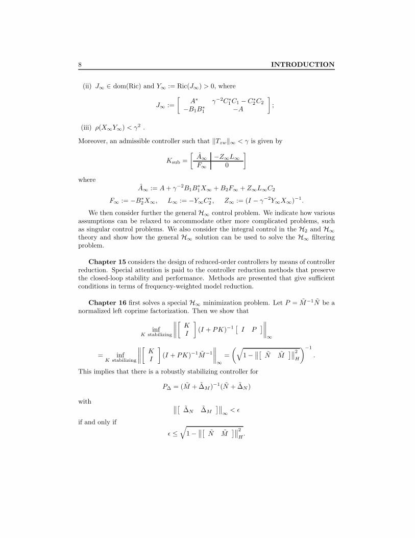
(ii) J∞ ∈ dom(Ric) and Y∞ := Ric(J∞) > 0, where
J∞ :=[
A∗ γ−2C∗1C1 − C∗2C2
−B1B∗1 −A
];
(iii) ρ(X∞Y∞) < γ2 .
Moreover, an admissible controller such that ‖Tzw‖∞ < γ is given by
Ksub =[A∞ −Z∞L∞F∞ 0
]where
A∞ := A+ γ−2B1B∗1X∞ +B2F∞ + Z∞L∞C2
F∞ := −B∗2X∞, L∞ := −Y∞C∗2 , Z∞ := (I − γ−2Y∞X∞)−1.
We then consider further the general H∞ control problem. We indicate how variousassumptions can be relaxed to accommodate other more complicated problems, suchas singular control problems. We also consider the integral control in the H2 and H∞theory and show how the general H∞ solution can be used to solve the H∞ filteringproblem.
Chapter 15 considers the design of reduced-order controllers by means of controllerreduction. Special attention is paid to the controller reduction methods that preservethe closed-loop stability and performance. Methods are presented that give sufficientconditions in terms of frequency-weighted model reduction.
Chapter 16 first solves a special H∞ minimization problem. Let P = M−1N be anormalized left coprime factorization. Then we show that
infK stabilizing
∥∥∥∥[ KI
](I + PK)−1
[I P
]∥∥∥∥∞
= infK stabilizing
∥∥∥∥[ KI
](I + PK)−1M−1
∥∥∥∥∞
=(√
1−∥∥[ N M
]∥∥2
H
)−1
.
This implies that there is a robustly stabilizing controller for
P∆ = (M + ∆M )−1(N + ∆N )
with ∥∥[ ∆N ∆M
]∥∥∞ < ε
if and only if
ε ≤√
1−∥∥[ N M
]∥∥2
H.

1.3. Notes and References 9
Using this stabilization result, a loop-shaping design technique is proposed. The pro-posed technique uses only the basic concept of loop-shaping methods, and then a robuststabilization controller for the normalized coprime factor perturbed system is used toconstruct the final controller.
Chapter 17 introduces the gap metric and the ν-gap metric. The frequency domaininterpretation and applications of the ν-gap metric are discussed. The controller orderreduction in the gap or ν-gap metric framework is also considered.
Chapter 18 considers briefly the problems of model validation and the mixed realand complex µ analysis and synthesis.
Most computations and examples in this book are done using Matlab. Since weshall use Matlab as a major computational tool, it is assumed that readers have somebasic working knowledge of the Matlab operations (for example, how to input vec-tors and matrices). We have also included in this book some brief explanations ofMatlab, Simulink
R , Control System Toolbox, and µ Analysis and Synthesis Toolbox1
commands. In particular, this book is written consistently with the µ Analysis andSynthesis Toolbox. (Robust Control Toolbox, LMI Control Toolbox, and other soft-ware packages may equally be used with this book.) Thus it is helpful for readers tohave access to this toolbox. It is suggested at this point to try the following demoprograms from this toolbox.
msdemo1
msdemo2
We shall introduce many more Matlab commands in the subsequent chapters.
1.3 Notes and References
The original formulation of the H∞ control problem can be found in Zames [1981].Relations between H∞ have now been established with many other topics in control:for example, risk-sensitive control of Whittle [1990]; differential games (see Basar andBernhard [1991], Limebeer, Anderson, Khargonekar, and Green [1992]; Green and Lime-beer [1995]); chain-scattering representation, and J-lossless factorization (Green [1992]and Kimura [1997]). See also Zhou, Doyle, and Glover [1996] for additional discussionsand references. The state-space theory of H∞ has also been carried much further, bygeneralizing time invariant to time varying, infinite horizon to finite horizon, and finitedimensional to infinite dimensional, and even to some nonlinear settings.
1Simulink is a registered trademark of The MathWorks, Inc.; µ-Analysis and Synthesis is a trade-mark of The MathWorks, Inc. and MUSYN Inc.; Control System Toolbox, Robust Control Toolbox,and LMI Control Toolbox are trademarks of The MathWorks, Inc.

10 INTRODUCTION
1.4 Problems
Problem 1.1 We shall solve an easy problem first. When you read a paper or a book,you often come across a statement like this “It is easy ...”. What the author reallymeant was one of the following: (a) it is really easy; (b) it seems to be easy; (c) it iseasy for an expert; (d) the author does not know how to show it but he or she thinks itis correct. Now prove that when I say “It is easy” in this book, I mean it is really easy.(Hint: If you can prove it after you read the whole book, ask your boss for a promotion.If you cannot prove it after you read the whole book, trash the book and write a bookyourself. Remember use something like “it is easy ...” if you are not sure what you aretalking about.)

Chapter 2
Linear Algebra
Some basic linear algebra facts will be reviewed in this chapter. The detailed treatmentof this topic can be found in the references listed at the end of the chapter. Hence we shallomit most proofs and provide proofs only for those results that either cannot be easilyfound in the standard linear algebra textbooks or are insightful to the understanding ofsome related problems.
2.1 Linear Subspaces
Let R denote the real scalar field and C the complex scalar field. For the interest of thischapter, let F be either R or C and let Fn be the vector space over F (i.e., Fn is either Rnor Cn). Now let x1, x2, . . . , xk ∈ Fn. Then an element of the form α1x1 +. . .+αkxk withαi ∈ F is a linear combination over F of x1, . . . , xk. The set of all linear combinationsof x1, x2, . . . , xk ∈ Fn is a subspace called the span of x1, x2, . . . , xk, denoted by
spanx1, x2, . . . , xk := x = α1x1 + . . .+ αkxk : αi ∈ F.
A set of vectors x1, x2, . . . , xk ∈ Fn is said to be linearly dependent over F if thereexists α1, . . . , αk ∈ F not all zero such that α1x2 + . . .+αkxk = 0; otherwise the vectorsare said to be linearly independent.
Let S be a subspace of Fn, then a set of vectors x1, x2, . . . , xk ∈ S is called a basisfor S if x1, x2, . . . , xk are linearly independent and S = spanx1, x2, . . . , xk. However,such a basis for a subspace S is not unique but all bases for S have the same numberof elements. This number is called the dimension of S, denoted by dim(S).
A set of vectors x1, x2, . . . , xk in Fn is mutually orthogonal if x∗i xj = 0 for alli 6= j and orthonormal if x∗i xj = δij , where the superscript ∗ denotes complex conjugatetranspose and δij is the Kronecker delta function with δij = 1 for i = j and δij = 0for i 6= j. More generally, a collection of subspaces S1, S2, . . . , Sk of Fn is mutuallyorthogonal if x∗y = 0 whenever x ∈ Si and y ∈ Sj for i 6= j.
11

12 LINEAR ALGEBRA
The orthogonal complement of a subspace S ⊂ Fn is defined by
S⊥ := y ∈ Fn : y∗x = 0 for all x ∈ S.
We call a set of vectors u1, u2, . . . , uk an orthonormal basis for a subspace S ∈ Fn ifthe vectors form a basis of S and are orthonormal. It is always possible to extend sucha basis to a full orthonormal basis u1, u2, . . . , un for Fn. Note that in this case
S⊥ = spanuk+1, . . . , un,
and uk+1, . . . , un is called an orthonormal completion of u1, u2, . . . , uk.Let A ∈ Fm×n be a linear transformation from Fn to Fm; that is,
A : Fn 7−→ Fm.
Then the kernel or null space of the linear transformation A is defined by
KerA = N(A) := x ∈ Fn : Ax = 0,
and the image or range of A is
ImA = R(A) := y ∈ Fm : y = Ax, x ∈ Fn.
Let ai, i = 1, 2, . . . , n denote the columns of a matrix A ∈ Fm×n; then
ImA = spana1, a2, . . . , an.
A square matrix U ∈ Fn×n whose columns form an orthonormal basis for Fn is calleda unitary matrix (or orthogonal matrix if F = R), and it satisfies U∗U = I = UU∗.
Now let A = [aij ] ∈ Cn×n; then the trace of A is defined as
trace(A) :=n∑i=1
aii.
Illustrative MATLAB Commands:
basis of KerA = null(A); basis of ImA = orth(A); rank of A = rank(A);
2.2 Eigenvalues and Eigenvectors
Let A ∈ Cn×n; then the eigenvalues of A are the n roots of its characteristic polynomialp(λ) = det(λI − A). The maximal modulus of the eigenvalues is called the spectralradius, denoted by
ρ(A) := max1≤i≤n
|λi|
if λi is a root of p(λ), where, as usual, | · | denotes the magnitude. The real spectralradius of a matrix A, denoted by ρR(A), is the maximum modulus of the real eigenvalues

2.3. Matrix Inversion Formulas 13
of A; that is, ρR(A) := maxλi∈R
|λi| and ρR(A) := 0 if A has no real eigenvalues. A nonzero
vector x ∈ Cn that satisfiesAx = λx
is referred to as a right eigenvector of A. Dually, a nonzero vector y is called a lefteigenvector of A if
y∗A = λy∗.
In general, eigenvalues need not be real, and neither do their corresponding eigenvectors.However, if A is real and λ is a real eigenvalue of A, then there is a real eigenvectorcorresponding to λ. In the case that all eigenvalues of a matrix A are real, we willdenote λmax(A) for the largest eigenvalue of A and λmin(A) for the smallest eigenvalue.In particular, if A is a Hermitian matrix (i.e., A = A∗), then there exist a unitary matrixU and a real diagonal matrix Λ such that A = UΛU∗, where the diagonal elements ofΛ are the eigenvalues of A and the columns of U are the eigenvectors of A.
Lemma 2.1 Consider the Sylvester equation
AX +XB = C, (2.1)
where A ∈ Fn×n, B ∈ Fm×m, and C ∈ Fn×m are given matrices. There exists aunique solution X ∈ Fn×m if and only if λi(A) + λj(B) 6= 0, ∀i = 1, 2, . . . , n, andj = 1, 2, . . . ,m.
In particular, if B = A∗, equation (2.1) is called the Lyapunov equation; and thenecessary and sufficient condition for the existence of a unique solution is thatλi(A) + λj(A) 6= 0, ∀i, j = 1, 2, . . . , n.
Illustrative MATLAB Commands:
[V, D] = eig(A) % AV = V D
X=lyap(A,B,-C) % solving Sylvester equation.
2.3 Matrix Inversion Formulas
Let A be a square matrix partitioned as follows:
A :=[A11 A12
A21 A22
],
where A11 and A22 are also square matrices. Now suppose A11 is nonsingular; then Ahas the following decomposition:[
A11 A12
A21 A22
]=[
I 0A21A
−111 I
] [A11 00 ∆
][I A−1
11 A12
0 I
]

14 LINEAR ALGEBRA
with ∆ := A22 − A21A−111 A12, and A is nonsingular iff ∆ is nonsingular. Dually, if A22
is nonsingular, then[A11 A12
A21 A22
]=[I A12A
−122
0 I
] [∆ 00 A22
][I 0
A−122 A21 I
]with ∆ := A11 −A12A
−122 A21, and A is nonsingular iff ∆ is nonsingular. The matrix ∆
(∆) is called the Schur complement of A11 (A22) in A.
Moreover, if A is nonsingular, then[A11 A12
A21 A22
]−1
=[A−1
11 +A−111 A12∆−1A21A
−111 −A−1
11 A12∆−1
−∆−1A21A−111 ∆−1
]and [
A11 A12
A21 A22
]−1
=[
∆−1 −∆−1A12A−122
−A−122 A21∆−1 A−1
22 +A−122 A21∆−1A12A
−122
].
The preceding matrix inversion formulas are particularly simple if A is block trian-gular: [
A11 0A21 A22
]−1
=[
A−111 0
−A−122 A21A
−111 A−1
22
][A11 A12
0 A22
]−1
=[A−1
11 −A−111 A12A
−122
0 A−122
].
The following identity is also very useful. Suppose A11 and A22 are both nonsingularmatrices; then
(A11 −A12A−122 A21)−1 = A−1
11 +A−111 A12(A22 −A21A
−111 A12)−1A21A
−111 .
As a consequence of the matrix decomposition formulas mentioned previously, wecan calculate the determinant of a matrix by using its submatrices. Suppose A11 isnonsingular; then
detA = detA11 det(A22 −A21A−111 A12).
On the other hand, if A22 is nonsingular, then
detA = detA22 det(A11 −A12A−122 A21).
In particular, for any B ∈ Cm×n and C ∈ Cn×m, we have
det[Im B−C In
]= det(In + CB) = det(Im +BC)
and for x, y ∈ Cndet(In + xy∗) = 1 + y∗x.
Related MATLAB Commands: inv, det
2.4. Invariant Subspaces 15
2.4 Invariant Subspaces
Let A : Cn 7−→ Cn be a linear transformation, λ be an eigenvalue of A, and x be acorresponding eigenvector, respectively. Then Ax = λx and A(αx) = λ(αx) for anyα ∈ C. Clearly, the eigenvector x defines a one-dimensional subspace that is invariantwith respect to premultiplication by A since Akx = λkx,∀k. In general, a subspaceS ⊂ Cn is called invariant for the transformation A, or A-invariant, if Ax ∈ S for everyx ∈ S. In other words, that S is invariant for A means that the image of S under Ais contained in S: AS ⊂ S. For example, 0, Cn, KerA, and ImA are all A-invariantsubspaces.
As a generalization of the one-dimensional invariant subspace induced by an eigen-vector, let λ1, . . . , λk be eigenvalues of A (not necessarily distinct), and let xi be the cor-responding eigenvectors and the generalized eigenvectors. Then S = spanx1, . . . , xkis an A-invariant subspace provided that all the lower-rank generalized eigenvectorsare included. More specifically, let λ1 = λ2 = · · · = λl be eigenvalues of A, andlet x1, x2, . . . , xl be the corresponding eigenvector and the generalized eigenvectors ob-tained through the following equations:
(A− λ1I)x1 = 0(A− λ1I)x2 = x1
...(A− λ1I)xl = xl−1.
Then a subspace S with xt ∈ S for some t ≤ l is an A-invariant subspace only if all lower-rank eigenvectors and generalized eigenvectors of xt are in S (i.e., xi ∈ S, ∀1 ≤ i ≤ t).This will be further illustrated in Example 2.1.
On the other hand, if S is a nontrivial subspace1 and is A-invariant, then there isx ∈ S and λ such that Ax = λx.
An A-invariant subspace S ⊂ Cn is called a stable invariant subspace if all theeigenvalues of A constrained to S have negative real parts. Stable invariant subspaceswill play an important role in computing the stabilizing solutions to the algebraic Riccatiequations in Chapter 12.
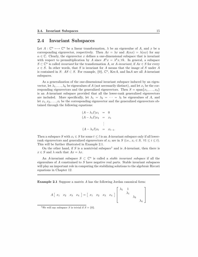
Example 2.1 Suppose a matrix A has the following Jordan canonical form:
A[x1 x2 x3 x4
]=[x1 x2 x3 x4
] λ1 1
λ1
λ3
λ4
1We will say subspace S is trivial if S = 0.

16 LINEAR ALGEBRA
with Reλ1 < 0, λ3 < 0, and λ4 > 0. Then it is easy to verify that
S1 = spanx1 S12 = spanx1, x2 S123 = spanx1, x2, x3S3 = spanx3 S13 = spanx1, x3 S124 = spanx1, x2, x4S4 = spanx4 S14 = spanx1, x4 S34 = spanx3, x4
are all A-invariant subspaces. Moreover, S1, S3, S12, S13, and S123 are stable A-invariantsubspaces. The subspaces S2 = spanx2, S23 = spanx2, x3, S24 = spanx2, x4, andS234 = spanx2, x3, x4 are, however, not A-invariant subspaces since the lower-rankeigenvector x1 is not in these subspaces. To illustrate, consider the subspace S23. Thenby definition, Ax2 ∈ S23 if it is an A-invariant subspace. Since
Ax2 = λx2 + x1,
Ax2 ∈ S23 would require that x1 be a linear combination of x2 and x3, but this isimpossible since x1 is independent of x2 and x3.
2.5 Vector Norms and Matrix Norms
In this section, we shall define vector and matrix norms. Let X be a vector space.A real-valued function ‖·‖ defined on X is said to be a norm on X if it satisfies thefollowing properties:
(i) ‖x‖ ≥ 0 (positivity);
(ii) ‖x‖ = 0 if and only if x = 0 (positive definiteness);
(iii) ‖αx‖ = |α| ‖x‖, for any scalar α (homogeneity);
(iv) ‖x+ y‖ ≤ ‖x‖+ ‖y‖ (triangle inequality)
for any x ∈ X and y ∈ X .
Let x ∈ Cn. Then we define the vector p-norm of x as
‖x‖p :=
(n∑i=1
|xi|p)1/p
, for 1 ≤ p <∞.
In particular, when p = 1, 2,∞ we have
‖x‖1 :=n∑i=1
|xi|;
‖x‖2 :=
√√√√ n∑i=1
|xi|2;

2.5. Vector Norms and Matrix Norms 17
‖x‖∞ := max1≤i≤n
|xi|.
Clearly, norm is an abstraction and extension of our usual concept of length in three-dimensional Euclidean space. So a norm of a vector is a measure of the vector “length”(for example, ‖x‖2 is the Euclidean distance of the vector x from the origin). Similarly,we can introduce some kind of measure for a matrix.
Let A = [aij ] ∈ Cm×n; then the matrix norm induced by a vector p-norm is definedas
‖A‖p := supx 6=0
‖Ax‖p‖x‖p
.
The matrix norms induced by vector p-norms are sometimes called induced p-norms.This is because ‖A‖p is defined by or induced from a vector p-norm. In fact, A canbe viewed as a mapping from a vector space Cn equipped with a vector norm ‖·‖p toanother vector space Cm equipped with a vector norm ‖·‖p. So from a system theoreticalpoint of view, the induced norms have the interpretation of input/output amplificationgains.
In particular, the induced matrix 2-norm can be computed as
‖A‖2 =√λmax(A∗A).
We shall adopt the following convention throughout this book for the vector andmatrix norms unless specified otherwise: Let x ∈ Cn and A ∈ Cm×n; then we shalldenote the Euclidean 2-norm of x simply by
‖x‖ := ‖x‖2
and the induced 2-norm of A by
‖A‖ := ‖A‖2 .
The Euclidean 2-norm has some very nice properties:
Lemma 2.2 Let x ∈ Fn and y ∈ Fm.
1. Suppose n ≥ m. Then ‖x‖ = ‖y‖ iff there is a matrix U ∈ Fn×m such that x = Uyand U∗U = I.
2. Suppose n = m. Then |x∗y| ≤ ‖x‖ ‖y‖. Moreover, the equality holds iff x = αyfor some α ∈ F or y = 0.
3. ‖x‖ ≤ ‖y‖ iff there is a matrix ∆ ∈ Fn×m with ‖∆‖ ≤ 1 such that x = ∆y.Furthermore, ‖x‖ < ‖y‖ iff ‖∆‖ < 1.
4. ‖Ux‖ = ‖x‖ for any appropriately dimensioned unitary matrices U .

18 LINEAR ALGEBRA
Another often used matrix norm is the so called Frobenius norm. It is defined as
‖A‖F :=√
trace(A∗A) =
√√√√ m∑i=1
n∑j=1
|aij |2 .
However, the Frobenius norm is not an induced norm.
The following properties of matrix norms are easy to show:
Lemma 2.3 Let A and B be any matrices with appropriate dimensions. Then
1. ρ(A) ≤ ‖A‖ (this is also true for the F -norm and any induced matrix norm).
2. ‖AB‖ ≤ ‖A‖ ‖B‖. In particular, this gives∥∥A−1
∥∥ ≥ ‖A‖−1 if A is invertible.(This is also true for any induced matrix norm.)
3. ‖UAV ‖ = ‖A‖, and ‖UAV ‖F = ‖A‖F , for any appropriately dimensioned unitarymatrices U and V .
4. ‖AB‖F ≤ ‖A‖ ‖B‖F and ‖AB‖F ≤ ‖B‖ ‖A‖F .
Note that although premultiplication or postmultiplication of a unitary matrix on amatrix does not change its induced 2-norm and F -norm, it does change its eigenvalues.For example, let
A =[
1 01 0
].
Then λ1(A) = 1, λ2(A) = 0. Now let
U =
[1√2
1√2
− 1√2
1√2
];
then U is a unitary matrix and
UA =[ √
2 00 0
]with λ1(UA) =
√2, λ2(UA) = 0. This property is useful in some matrix perturbation
problems, particularly in the computation of bounds for structured singular values,which will be studied in Chapter 9.
Related MATLAB Commands: norm, normest

2.6. Singular Value Decomposition 19
2.6 Singular Value Decomposition
A very useful tool in matrix analysis is singular value decomposition (SVD). It will beseen that singular values of a matrix are good measures of the “size” of the matrix andthat the corresponding singular vectors are good indications of strong/weak input oroutput directions.
Theorem 2.4 Let A ∈ Fm×n. There exist unitary matrices
U = [u1, u2, . . . , um] ∈ Fm×m
V = [v1, v2, . . . , vn] ∈ Fn×n
such that
A = UΣV ∗, Σ =[
Σ1 00 0
],
where
Σ1 =
σ1 0 · · · 00 σ2 · · · 0...
.... . .
...0 0 · · · σp
and
σ1 ≥ σ2 ≥ · · · ≥ σp ≥ 0, p = minm,n.
Proof. Let σ = ‖A‖ and without loss of generality assume m ≥ n. Then, from thedefinition of ‖A‖, there exists a z ∈ Fn such that
‖Az‖ = σ ‖z‖ .
By Lemma 2.2, there is a matrix U ∈ Fm×n such that U∗U = I and
Az = σUz.
Now let
x =z
‖z‖ ∈ Fn, y =
Uz∥∥∥Uz∥∥∥ ∈ Fm.We have Ax = σy. Let
V =[x V1
]∈ Fn×n
andU =
[y U1
]∈ Fm×m
be unitary.2 Consequently, U∗AV has the following structure:
A1 := U∗AV =[y∗Ax y∗AV1
U∗1Ax U∗1AV1
]=[σy∗y y∗AV1
σU∗1 y U∗1AV1
]=[σ w∗
0 B
],
2Recall that it is always possible to extend an orthonormal set of vectors to an orthonormal basisfor the whole space.

20 LINEAR ALGEBRA
where w := V ∗1 A∗y ∈ Fn−1 and B := U∗1AV1 ∈ F(m−1)×(n−1).
Since ∥∥∥∥∥∥∥∥∥A∗1
10...0
∥∥∥∥∥∥∥∥∥
2
2
= (σ2 + w∗w),
it follows that ‖A1‖2 ≥ σ2 + w∗w. But since σ = ‖A‖ = ‖A1‖, we must have w = 0.An obvious induction argument gives
U∗AV = Σ.
This completes the proof. 2
The σi is the ith singular value of A, and the vectors ui and vj are, respectively,the ith left singular vector and the jth right singular vector. It is easy to verify that
Avi = σiui
A∗ui = σivi.
The preceding equations can also be written as
A∗Avi = σ2i vi
AA∗ui = σ2i ui.
Hence σ2i is an eigenvalue of AA∗ or A∗A, ui is an eigenvector of AA∗, and vi is an
eigenvector of A∗A.The following notations for singular values are often adopted:
σ(A) = σmax(A) = σ1 = the largest singular value of A;
andσ(A) = σmin(A) = σp = the smallest singular value of A.
Geometrically, the singular values of a matrix A are precisely the lengths of the semi-axes of the hyperellipsoid E defined by
E = y : y = Ax, x ∈ Cn, ‖x‖ = 1.
Thus v1 is the direction in which ‖y‖ is largest for all ‖x‖ = 1; while vn is the directionin which ‖y‖ is smallest for all ‖x‖ = 1. From the input/output point of view, v1 (vn)is the highest (lowest) gain input (or control) direction, while u1 (um) is the highest(lowest) gain output (or observing) direction. This can be illustrated by the following2× 2 matrix:
A =[
cos θ1 − sin θ1
sin θ1 cos θ1
] [σ1
σ2
][cos θ2 − sin θ2
sin θ2 cos θ2
].

2.6. Singular Value Decomposition 21
It is easy to see that A maps a unit circle to an ellipsoid with semiaxes of σ1 and σ2.
Hence it is often convenient to introduce the following alternative definitions for thelargest singular value σ:
σ(A) := max‖x‖=1
‖Ax‖
and for the smallest singular value σ of a tall matrix:
σ(A) := min‖x‖=1
‖Ax‖ .
Lemma 2.5 Suppose A and ∆ are square matrices. Then
(i) |σ(A+ ∆)− σ(A)| ≤ σ(∆);
(ii) σ(A∆) ≥ σ(A)σ(∆);
(iii) σ(A−1) =1
σ(A)if A is invertible.
Proof.
(i) By definition
σ(A+ ∆) := min‖x‖=1
‖(A+ ∆)x‖ ≥ min‖x‖=1
‖Ax‖ − ‖∆x‖
≥ min‖x‖=1
‖Ax‖ − max‖x‖=1
‖∆x‖
= σ(A)− σ(∆).
Hence −σ(∆) ≤ σ(A+ ∆)−σ(A). The other inequality σ(A+ ∆)−σ(A) ≤ σ(∆)follows by replacing A by A+ ∆ and ∆ by −∆ in the preceding proof.
(ii) This follows by noting that
σ(A∆) := min‖x‖=1
‖A∆x‖
=√
min‖x‖=1
x∗∆∗A∗A∆x
≥ σ(A) min‖x‖=1
‖∆x‖ = σ(A)σ(∆).
(iii) Let the singular value decomposition of A be A = UΣV ∗; then A−1 = V Σ−1U∗.Hence σ(A−1) = σ(Σ−1) = 1/σ(Σ) = 1/σ(A).
2
Note that (ii) may not be true if A and ∆ are not square matrices. For example,
consider A =[
12
]and ∆ =
[3 4
]; then σ(A∆) = 0 but σ(A) =
√5 and σ(∆) = 5.

22 LINEAR ALGEBRA
Some useful properties of SVD are collected in the following lemma.
Lemma 2.6 Let A ∈ Fm×n and
σ1 ≥ σ2 ≥ · · · ≥ σr > σr+1 = · · · = 0, r ≤ minm,n.
Then
1. rank(A) = r;
2. KerA = spanvr+1, . . . , vn and (KerA)⊥ = spanv1, . . . , vr;
3. ImA = spanu1, . . . , ur and (ImA)⊥ = spanur+1, . . . , um;
4. A ∈ Fm×n has a dyadic expansion:
A =r∑i=1
σiuiv∗i = UrΣrV ∗r ,
where Ur = [u1, . . . , ur], Vr = [v1, . . . , vr], and Σr = diag (σ1, . . . , σr);
5. ‖A‖2F = σ21 + σ2
2 + · · ·+ σ2r ;
6. ‖A‖ = σ1;
7. σi(U0AV0) = σi(A), i = 1, . . . , p for any appropriately dimensioned unitary ma-trices U0 and V0;
8. Let k < r = rank(A) and Ak :=∑ki=1 σiuiv
∗i ; then
minrank(B)≤k
‖A−B‖ = ‖A−Ak‖ = σk+1.
Proof. We shall only give a proof for part 8. It is easy to see that rank(Ak) ≤ k and‖A−Ak‖ = σk+1. Hence, we only need show that min
rank(B)≤k‖A−B‖ ≥ σk+1. Let B
be any matrix such that rank(B) ≤ k. Then
‖A−B‖ = ‖UΣV ∗ −B‖ = ‖Σ− U∗BV ‖
≥∥∥∥∥[ Ik+1 0
](Σ− U∗BV )
[Ik+1
0
]∥∥∥∥ =∥∥∥Σk+1 − B
∥∥∥ ,where B =
[Ik+1 0
]U∗BV
[Ik+1
0
]∈ F(k+1)×(k+1) and rank(B) ≤ k. Let x ∈ Fk+1
be such that Bx = 0 and ‖x‖ = 1. Then
‖A−B‖ ≥∥∥∥Σk+1 − B
∥∥∥ ≥ ∥∥∥(Σk+1 − B)x∥∥∥ = ‖Σk+1x‖ ≥ σk+1.
Since B is arbitrary, the conclusion follows. 2

2.7. Semidefinite Matrices 23
Illustrative MATLAB Commands:
[U,Σ,V] = svd(A) % A = UΣV ∗
Related MATLAB Commands: cond, condest
2.7 Semidefinite Matrices
A square Hermitian matrix A = A∗ is said to be positive definite (semidefinite), denotedby A > 0 (≥ 0), if x∗Ax > 0 (≥ 0) for all x 6= 0. Suppose A ∈ Fn×n and A = A∗ ≥ 0;then there exists a B ∈ Fn×r with r ≥ rank(A) such that A = BB∗.
Lemma 2.7 Let B ∈ Fm×n and C ∈ Fk×n. Suppose m ≥ k and B∗B = C∗C. Thenthere exists a matrix U ∈ Fm×k such that U∗U = I and B = UC.
Proof. Let V1 and V2 be unitary matrices such that
B = V1
[B1
0
], C = V2
[C1
0
],
where B1 and C1 are full-row rank. Then B1 and C1 have the same number of rowsand V3 := B1C
∗1 (C1C
∗1 )−1 satisfies V ∗3 V3 = I since B∗B = C∗C. Hence V3 is a unitary
matrix and V ∗3 B1 = C1. Finally, let
U = V1
[V3 00 V4
]V ∗2
for any suitably dimensioned V4 such that V ∗4 V4 = I. 2
We can define square root for a positive semidefinite matrix A, A1/2 = (A1/2)∗ ≥ 0,by
A = A1/2A1/2.
Clearly, A1/2 can be computed by using spectral decomposition or SVD: Let A = UΛU∗;then
A1/2 = UΛ1/2U∗,
whereΛ = diagλ1, . . . , λn, Λ1/2 = diag
√λ1, . . . ,
√λn.

24 LINEAR ALGEBRA
Lemma 2.8 Suppose A = A∗ > 0 and B = B∗ ≥ 0. Then A > B iff ρ(BA−1) < 1.
Proof. Since A > 0, we have A > B iff
0 < I −A−1/2BA−1/2
i.e., iff ρ(A−1/2BA−1/2) < 1. However, A−1/2BA−1/2 and BA−1 are similar, henceρ(BA−1) = ρ(A−1/2BA−1/2) and the claim follows. 2
2.8 Notes and References
A very extensive treatment of most topics in this chapter can be found in Brogan [1991],Horn and Johnson [1990, 1991] and Lancaster and Tismenetsky [1985]. Golub and VanLoan’s book [1983] contains many numerical algorithms for solving most of the problemsin this chapter.
2.9 Problems
Problem 2.1 Let
A =
1 1 01 0 12 1 11 0 12 0 2
.
Determine the row and column rank of A and find bases for Im(A), Im(A∗), and Ker(A).
Problem 2.2 Let D0 =
1 42 53 6
. Find a D such that D∗D = I and ImD = ImD0.
Furthermore, find a D⊥ such that[D D⊥
]is a unitary matrix.
Problem 2.3 Let A be a nonsingular matrix and x, y ∈ Cn. Show
(A−1 + xy∗)−1 = A− Axy∗A
1 + y∗Ax
anddet(A−1 + xy∗)−1 =
detA1 + y∗Ax
.
Problem 2.4 Let A and B be compatible matrices. Show
B(I +AB)−1 = (I +BA)−1B, (I +A)−1 = I −A(I +A)−1.

2.9. Problems 25
Problem 2.5 Find a basis for the maximum dimensional stable invariant subspace of
H =[
A R−Q −A∗
]with
1. A =[−1 23 0
], R =
[−1 −1−1 −1
], and Q = 0
2. A =[
0 10 2
], R =
[0 00 −1
], and Q =
[1 22 4
]
3. A = 0, R =[
1 22 5
], and Q = I2.
Problem 2.6 Let A = [aij ]. Show that α(A) := maxi,j |aij | defines a matrix norm.Give examples so that α(A) < ρ(A) and α(AB) > α(A)α(B).
Problem 2.7 Let A =(
1 2 34 1 −1
)and B =
(01
). (a) Find all x such that Ax = B.
(b) Find the minimal norm solution x: min ‖x‖ : Ax = B.
Problem 2.8 Let A =
1 2−2 −50 1
and B =
345
. Find an x such that ‖Ax−B‖
is minimized.
Problem 2.9 Let ‖A‖ < 1. Show
1. (I −A)−1 = I +A+A2 + · · · .
2.∥∥(I −A)−1
∥∥ ≤ 1 + ‖A‖+ ‖A‖2 + · · · = 11−‖A‖ .
3.∥∥(I −A)−1
∥∥ ≥ 11+‖A‖ .
Problem 2.10 Let A ∈ Cm×n. Show that
1√m‖A‖2 ≤ ‖A‖∞ ≤
√n ‖A‖2 ;
1√n‖A‖2 ≤ ‖A‖1 ≤
√m ‖A‖2 ;
1n‖A‖∞ ≤ ‖A‖1 ≤ m ‖A‖∞ .
Problem 2.11 Let A = xy∗ and x, y ∈ Cn. Show that ‖A‖2 = ‖A‖F = ‖x‖ ‖y‖.
Problem 2.12 Let A =[
1 1 + j1− j 2
]. Find A
12 and a B ∈ C2 such that A = BB∗.
26 LINEAR ALGEBRA
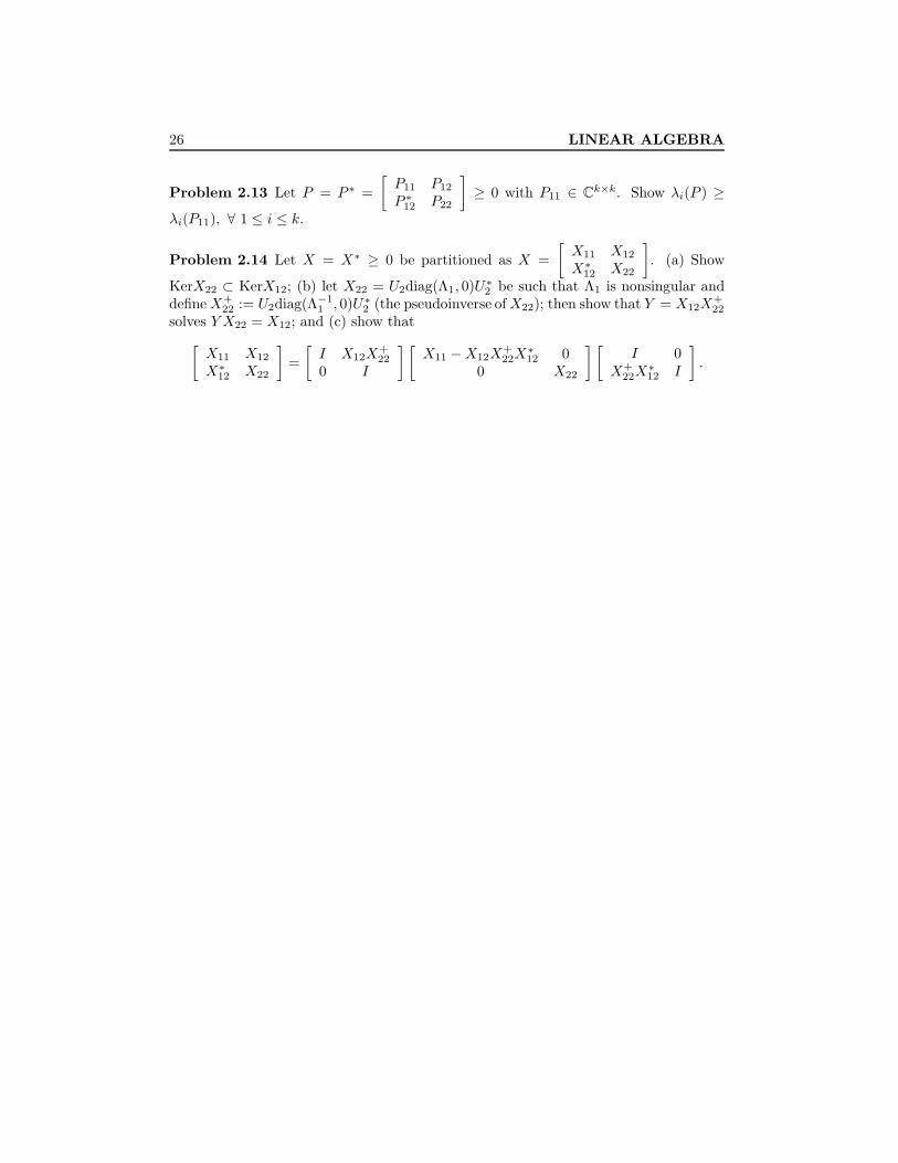
Problem 2.13 Let P = P ∗ =[P11 P12
P ∗12 P22
]≥ 0 with P11 ∈ Ck×k. Show λi(P ) ≥
λi(P11), ∀ 1 ≤ i ≤ k.
Problem 2.14 Let X = X∗ ≥ 0 be partitioned as X =[X11 X12
X∗12 X22
]. (a) Show
KerX22 ⊂ KerX12; (b) let X22 = U2diag(Λ1, 0)U∗2 be such that Λ1 is nonsingular anddefineX+
22 := U2diag(Λ−11 , 0)U∗2 (the pseudoinverse ofX22); then show that Y = X12X
+22
solves Y X22 = X12; and (c) show that[X11 X12
X∗12 X22
]=[I X12X
+22
0 I
][X11 −X12X
+22X
∗12 0
0 X22
] [I 0
X+22X
∗12 I
].

Chapter 3
Linear Systems
This chapter reviews some basic system theoretical concepts. The notions of controlla-bility, observability, stabilizability, and detectability are defined and various algebraicand geometric characterizations of these notions are summarized. Observer theory isthen introduced. System interconnections and realizations are studied. Finally, theconcepts of system poles and zeros are introduced.
3.1 Descriptions of Linear Dynamical Systems
Let a finite dimensional linear time invariant (FDLTI) dynamical system be describedby the following linear constant coefficient differential equations:
x = Ax+Bu, x(t0) = x0 (3.1)y = Cx+Du, (3.2)
where x(t) ∈ Rn is called the system state, x(t0) is called the initial condition of thesystem, u(t) ∈ Rm is called the system input, and y(t) ∈ Rp is the system output. TheA,B,C, and D are appropriately dimensioned real constant matrices. A dynamicalsystem with single-input (m = 1) and single-output (p = 1) is called a SISO (single-input and single-output) system; otherwise it is called a MIMO (multiple-input andmultiple-output) system. The corresponding transfer matrix from u to y is defined as
Y (s) = G(s)U(s),
where U(s) and Y (s) are the Laplace transforms of u(t) and y(t) with zero initialcondition (x(0) = 0). Hence, we have
G(s) = C(sI −A)−1B +D.
Note that the system equations (3.1) and (3.2) can be written in a more compact matrixform: [
xy
]=[A BC D
] [xu
].
27
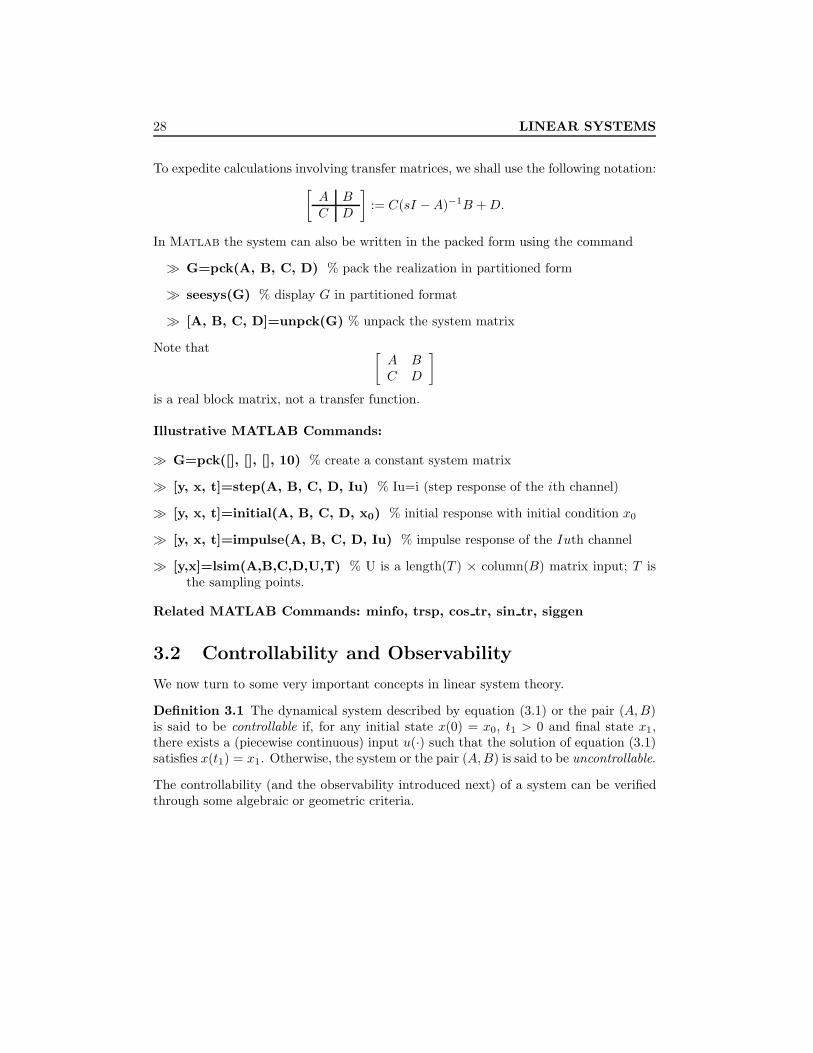
28 LINEAR SYSTEMS
To expedite calculations involving transfer matrices, we shall use the following notation:[A BC D
]:= C(sI −A)−1B +D.
In Matlab the system can also be written in the packed form using the command
G=pck(A, B, C, D) % pack the realization in partitioned form
seesys(G) % display G in partitioned format
[A, B, C, D]=unpck(G) % unpack the system matrix
Note that [A BC D
]is a real block matrix, not a transfer function.
Illustrative MATLAB Commands:
G=pck([], [], [], 10) % create a constant system matrix
[y, x, t]=step(A, B, C, D, Iu) % Iu=i (step response of the ith channel)
[y, x, t]=initial(A, B, C, D, x0) % initial response with initial condition x0
[y, x, t]=impulse(A, B, C, D, Iu) % impulse response of the Iuth channel
[y,x]=lsim(A,B,C,D,U,T) % U is a length(T ) × column(B) matrix input; T isthe sampling points.
Related MATLAB Commands: minfo, trsp, cos tr, sin tr, siggen
3.2 Controllability and Observability
We now turn to some very important concepts in linear system theory.
Definition 3.1 The dynamical system described by equation (3.1) or the pair (A,B)is said to be controllable if, for any initial state x(0) = x0, t1 > 0 and final state x1,there exists a (piecewise continuous) input u(·) such that the solution of equation (3.1)satisfies x(t1) = x1. Otherwise, the system or the pair (A,B) is said to be uncontrollable.
The controllability (and the observability introduced next) of a system can be verifiedthrough some algebraic or geometric criteria.

3.2. Controllability and Observability 29
Theorem 3.1 The following are equivalent:
(i) (A,B) is controllable.
(ii) The matrix
Wc(t) :=∫ t
0
eAτBB∗eA∗τdτ
is positive definite for any t > 0.
(iii) The controllability matrix
C =[B AB A2B . . . An−1B
]has full-row rank or, in other words, 〈A |ImB〉 :=
∑ni=1 Im(Ai−1B) = Rn.
(iv) The matrix [A− λI, B] has full-row rank for all λ in C.
(v) Let λ and x be any eigenvalue and any corresponding left eigenvector of A (i.e.,x∗A = x∗λ); then x∗B 6= 0.
(vi) The eigenvalues of A+BF can be freely assigned (with the restriction that complexeigenvalues are in conjugate pairs) by a suitable choice of F .
Example 3.1 Let A =[
2 00 2
]and B =
[11
]. Then x1 =
[10
]and x2 =
[01
]are independent eigenvectors of A and x∗iB 6= 0, i = 1, 2. However, this should not leadone to conclude that (A,B) is controllable. In fact, x = x1 − x2 is also an eigenvectorof A and x∗B = 0, which implies that (A,B) is not controllable. Hence one must checkfor all possible eigenvectors in using criterion (v).
Definition 3.2 An unforced dynamical system x = Ax is said to be stable if all theeigenvalues of A are in the open left half plane; that is, Reλ(A) < 0. A matrix A withsuch a property is said to be stable or Hurwitz.
Definition 3.3 The dynamical system of equation (3.1), or the pair (A, B), is said tobe stabilizable if there exists a state feedback u = Fx such that the system is stable(i.e., A+BF is stable).
It is more appropriate to call this stabilizability the state feedback stabilizability todifferentiate it from the output feedback stabilizability defined later.
The following theorem is a consequence of Theorem 3.1.

30 LINEAR SYSTEMS
Theorem 3.2 The following are equivalent:
(i) (A, B) is stabilizable.
(ii) The matrix [A− λI, B] has full-row rank for all Reλ ≥ 0.
(iii) For all λ and x such that x∗A = x∗λ and Reλ ≥ 0, x∗B 6= 0.
(iv) There exists a matrix F such that A+BF is Hurwitz.
We now consider the dual notions: observability and detectability of the systemdescribed by equations (3.1) and (3.2).
Definition 3.4 The dynamical system described by equations (3.1) and (3.2) or by thepair (C,A) is said to be observable if, for any t1 > 0, the initial state x(0) = x0 can bedetermined from the time history of the input u(t) and the output y(t) in the intervalof [0, t1]. Otherwise, the system, or (C,A), is said to be unobservable.
Theorem 3.3 The following are equivalent:
(i) (C,A) is observable.
(ii) The matrix
Wo(t) :=∫ t
0
eA∗τC∗CeAτdτ
is positive definite for any t > 0.
(iii) The observability matrix
O =
CCACA2
...CAn−1
has full-column rank or
⋂ni=1 Ker(CAi−1) = 0.
(iv) The matrix[A− λIC
]has full-column rank for all λ in C.
(v) Let λ and y be any eigenvalue and any corresponding right eigenvector of A (i.e.,Ay = λy); then Cy 6= 0.
(vi) The eigenvalues of A+LC can be freely assigned (with the restriction that complexeigenvalues are in conjugate pairs) by a suitable choice of L.
(vii) (A∗, C∗) is controllable.

3.3. Observers and Observer-Based Controllers 31
Definition 3.5 The system, or the pair (C,A), is detectable if A + LC is stable forsome L.
Theorem 3.4 The following are equivalent:
(i) (C,A) is detectable.
(ii) The matrix[A− λIC
]has full-column rank for all Reλ ≥ 0.
(iii) For all λ and x such that Ax = λx and Reλ ≥ 0, Cx 6= 0.
(iv) There exists a matrix L such that A+ LC is Hurwitz.
(v) (A∗, C∗) is stabilizable.
The conditions (iv) and (v) of Theorems 3.1 and 3.3 and the conditions (ii) and(iii) of Theorems 3.2 and 3.4 are often called Popov-Belevitch-Hautus (PBH) tests. Inparticular, the following definitions of modal controllability and observability are oftenuseful.
Definition 3.6 Let λ be an eigenvalue of A or, equivalently, a mode of the system.Then the mode λ is said to be controllable (observable) if x∗B 6= 0 (Cx 6= 0) for allleft (right) eigenvectors of A associated with λ; that is, x∗A = λx∗ (Ax = λx) and0 6= x ∈ Cn. Otherwise, the mode is said to be uncontrollable (unobservable).
It follows that a system is controllable (observable) if and only if every mode is control-lable (observable). Similarly, a system is stabilizable (detectable) if and only if everyunstable mode is controllable (observable).
Illustrative MATLAB Commands:
C= ctrb(A, B); O= obsv(A, C);
Wc(∞)=gram(A, B); % if A is stable.
F=-place(A, B, P) % P is a vector of desired eigenvalues.
Related MATLAB Commands: ctrbf, obsvf, canon, strans, acker
3.3 Observers and Observer-Based Controllers
It is clear that if a system is controllable and the system states are available for feed-back, then the system closed-loop poles can be assigned arbitrarily through a constantfeedback. However, in most practical applications, the system states are not completelyaccessible and all the designer knows are the output y and input u. Hence, the esti-mation of the system states from the given output information y and input u is often

32 LINEAR SYSTEMS
necessary to realize some specific design objectives. In this section, we consider such anestimation problem and the application of this state estimation in feedback control.
Consider a plant modeled by equations (3.1) and (3.2). An observer is a dynamicalsystem with input (u, y) and output (say, x), that asymptotically estimates the state x,that is, x(t)− x(t)→ 0 as t→∞ for all initial states and for every input.
Theorem 3.5 An observer exists iff (C,A) is detectable. Further, if (C,A) is de-tectable, then a full-order Luenberger observer is given by
q = Aq +Bu+ L(Cq +Du− y) (3.3)x = q, (3.4)
where L is any matrix such that A+ LC is stable.
Recall that, for a dynamical system described by the equations (3.1) and (3.2), if (A,B)is controllable and state x is available for feedback, then there is a state feedback u = Fxsuch that the closed-loop poles of the system can be arbitrarily assigned. Similarly, if(C,A) is observable, then the system observer poles can be arbitrarily placed so that thestate estimator x can be made to approach x arbitrarily fast. Now let us consider whatwill happen if the system states are not available for feedback so that the estimatedstate has to be used. Hence, the controller has the following dynamics:
˙x = (A+ LC)x+Bu+ LDu− Lyu = Fx.
Then the total system state equations are given by[x˙x
]=[
A BF−LC A+BF + LC
][xx
].
Let e := x− x; then the system equation becomes[e˙x
]=[A+ LC 0−LC A+BF
] [ex
]and the closed-loop poles consist of two parts: the poles resulting from state feedbackλi(A + BF ) and the poles resulting from the state estimation λj(A + LC). Now if(A,B) is controllable and (C,A) is observable, then there exist F and L such that theeigenvalues of A+BF and A+LC can be arbitrarily assigned. In particular, they canbe made to be stable. Note that a slightly weaker result can also result even if (A,B)and (C,A) are only stabilizable and detectable.
The controller given above is called an observer-based controller and is denoted as
u = K(s)y
and
K(s) =[A+BF + LC + LDF −L
F 0
].
3.3. Observers and Observer-Based Controllers 33
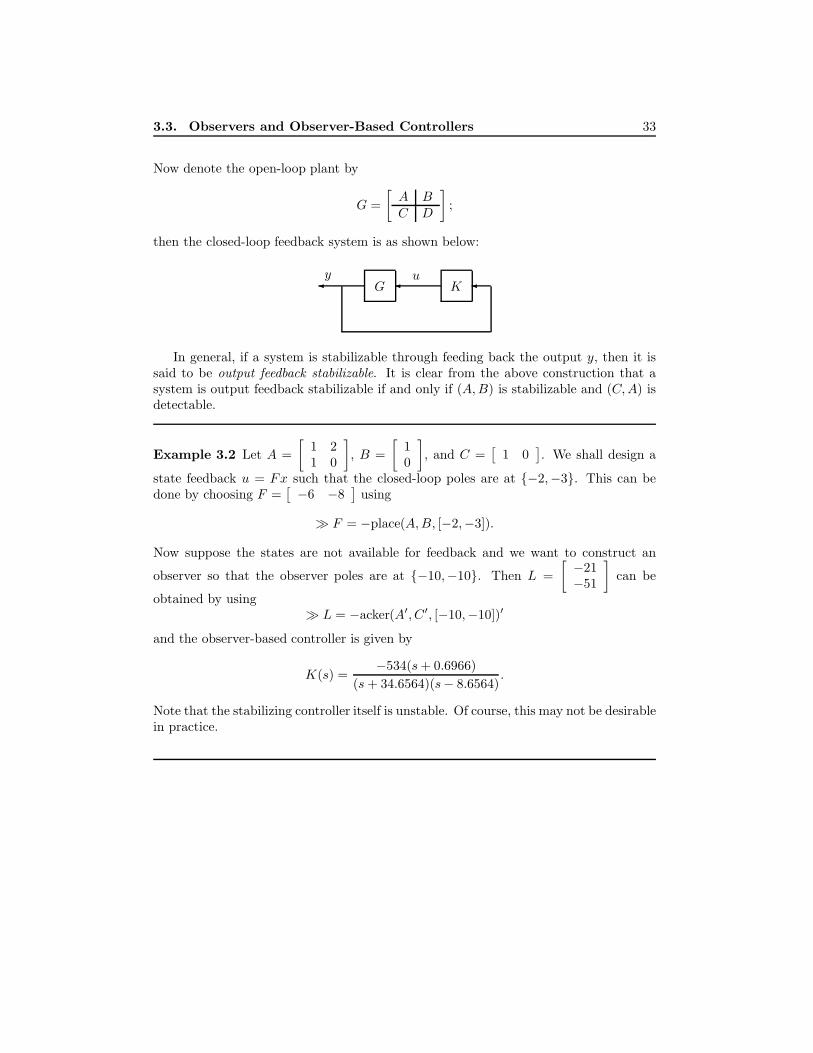
Now denote the open-loop plant by
G =[A BC D
];
then the closed-loop feedback system is as shown below:
G K y u
In general, if a system is stabilizable through feeding back the output y, then it issaid to be output feedback stabilizable. It is clear from the above construction that asystem is output feedback stabilizable if and only if (A,B) is stabilizable and (C,A) isdetectable.
Example 3.2 Let A =[
1 21 0
], B =
[10
], and C =
[1 0
]. We shall design a
state feedback u = Fx such that the closed-loop poles are at −2,−3. This can bedone by choosing F =
[−6 −8
]using
F = −place(A,B, [−2,−3]).
Now suppose the states are not available for feedback and we want to construct an
observer so that the observer poles are at −10,−10. Then L =[−21−51
]can be
obtained by using L = −acker(A′, C′, [−10,−10])′
and the observer-based controller is given by
K(s) =−534(s+ 0.6966)
(s+ 34.6564)(s− 8.6564).
Note that the stabilizing controller itself is unstable. Of course, this may not be desirablein practice.

34 LINEAR SYSTEMS
3.4 Operations on Systems
In this section, we present some facts about system interconnection. Since these proofsare straightforward, we will leave the details to the reader.
Suppose that G1 and G2 are two subsystems with state-space representations:
G1 =[A1 B1
C1 D1
], G2 =
[A2 B2
C2 D2
].
Then the series or cascade connection of these two subsystems is a system with theoutput of the second subsystem as the input of the first subsystem, as shown in thefollowing diagram:
G2G1
This operation in terms of the transfer matrices of the two subsystems is essentially theproduct of two transfer matrices. Hence, a representation for the cascaded system canbe obtained as
G1G2 =[A1 B1
C1 D1
] [A2 B2
C2 D2
]
=
A1 B1C2
0 A2
B1D2
B2
C1 D1C2 D1D2
=
A2 0B1C2 A1
B2
B1D2
D1C2 C1 D1D2
.Similarly, the parallel connection or the addition of G1 and G2 can be obtained as
G1 +G2 =[A1 B1
C1 D1
]+[A2 B2
C2 D2
]=
A1 00 A2
B1
B2
C1 C2 D1 +D2
.For future reference, we shall also introduce the following definitions.
Definition 3.7 The transpose of a transfer matrix G(s) or the dual system is definedas
G 7−→ GT (s) = B∗(sI −A∗)−1C∗ +D∗
or, equivalently, [A BC D
]7−→
[A∗ C∗
B∗ D∗
].
Definition 3.8 The conjugate system of G(s) is defined as
G 7−→ G∼(s) := GT (−s) = B∗(−sI −A∗)−1C∗ +D∗
or, equivalently, [A BC D
]7−→
[−A∗ −C∗B∗ D∗
].

3.5. State-Space Realizations for Transfer Matrices 35
In particular, we have G∗(jω) := [G(jω)]∗ = G∼(jω).
A real rational matrix G(s) is called an inverse of a transfer matrixG(s) ifG(s)G(s) =G(s)G(s) = I. Suppose G(s) is square and D is invertible. Then
G−1 =[A−BD−1C −BD−1
D−1C D−1
].
The corresponding Matlab commands are
G1G2 ⇐⇒ mmult(G1,G2),[G1 G2
]⇐⇒ sbs(G1,G2)
G1 +G2 ⇐⇒ madd(G1,G2), G1 −G2 ⇐⇒ msub(G1,G2)[G1
G2
]⇐⇒ abv(G1,G2),
[G1
G2
]⇐⇒ daug(G1,G2),
GT (s) ⇐⇒ transp(G), G∼(s) ⇐⇒ cjt(G), G−1(s) ⇐⇒ minv(G)
α G(s) ⇐⇒ mscl(G, α), α is a scalar.
Related MATLAB Commands: append, parallel, feedback, series, cloop,sclin, sclout, sel
3.5 State-Space Realizations for Transfer Matrices
In some cases, the natural or convenient description for a dynamical system is in termsof matrix transfer function. This occurs, for example, in some highly complex sys-tems for which the analytic differential equations are too hard or too complex to writedown. Hence certain engineering approximation or identification has to be carried out;for example, input and output frequency responses are obtained from experiments sothat some transfer matrix approximating the system dynamics can be obtained. Sincethe state-space computation is most convenient to implement on the computer, someappropriate state-space representation for the resulting transfer matrix is necessary.
In general, assume that G(s) is a real rational transfer matrix that is proper. Thenwe call a state-space model (A,B,C,D) such that
G(s) =[A BC D
]a realization of G(s).
Definition 3.9 A state-space realization (A,B,C,D) of G(s) is said to be a minimalrealization of G(s) if A has the smallest possible dimension.
Theorem 3.6 A state-space realization (A,B,C,D) of G(s) is minimal if and only if(A,B) is controllable and (C,A) is observable.
36 LINEAR SYSTEMS
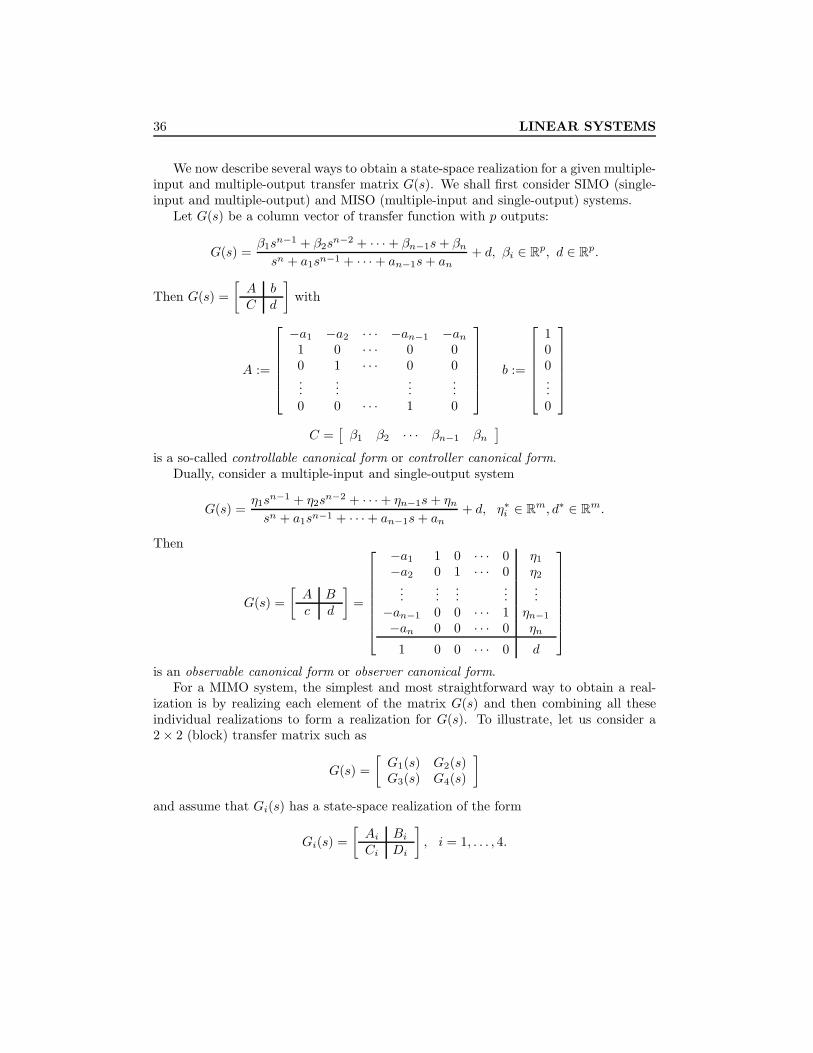
We now describe several ways to obtain a state-space realization for a given multiple-input and multiple-output transfer matrix G(s). We shall first consider SIMO (single-input and multiple-output) and MISO (multiple-input and single-output) systems.
Let G(s) be a column vector of transfer function with p outputs:
G(s) =β1s
n−1 + β2sn−2 + · · ·+ βn−1s+ βn
sn + a1sn−1 + · · ·+ an−1s+ an+ d, βi ∈ Rp, d ∈ Rp.
Then G(s) =[A bC d
]with
A :=
−a1 −a2 · · · −an−1 −an
1 0 · · · 0 00 1 · · · 0 0...
......
...0 0 · · · 1 0
b :=
100...0
C =
[β1 β2 · · · βn−1 βn
]is a so-called controllable canonical form or controller canonical form.
Dually, consider a multiple-input and single-output system
G(s) =η1s
n−1 + η2sn−2 + · · ·+ ηn−1s+ ηn
sn + a1sn−1 + · · ·+ an−1s+ an+ d, η∗i ∈ Rm, d∗ ∈ Rm.
Then
G(s) =[A Bc d
]=
−a1 1 0 · · · 0 η1
−a2 0 1 · · · 0 η2
......
......
...−an−1 0 0 · · · 1 ηn−1
−an 0 0 · · · 0 ηn
1 0 0 · · · 0 d
is an observable canonical form or observer canonical form.
For a MIMO system, the simplest and most straightforward way to obtain a real-ization is by realizing each element of the matrix G(s) and then combining all theseindividual realizations to form a realization for G(s). To illustrate, let us consider a2× 2 (block) transfer matrix such as
G(s) =[G1(s) G2(s)G3(s) G4(s)
]and assume that Gi(s) has a state-space realization of the form
Gi(s) =[Ai BiCi Di
], i = 1, . . . , 4.

3.5. State-Space Realizations for Transfer Matrices 37
Then a realization for G(s) can be obtained as (G = abv(sbs(G1,G2), sbs(G3,G4))):
G(s) =
A1 0 0 0 B1 00 A2 0 0 0 B2
0 0 A3 0 B3 00 0 0 A4 0 B4
C1 C2 0 0 D1 D2
0 0 C3 C4 D3 D4
.
Alternatively, if the transfer matrix G(s) can be factored into the product and/orthe sum of several simply realized transfer matrices, then a realization for G can beobtained by using the cascade or addition formulas given in the preceding section.
A problem inherited with these kinds of realization procedures is that a realizationthus obtained will generally not be minimal. To obtain a minimal realization, a Kalmancontrollability and observability decomposition has to be performed to eliminate the un-controllable and/or unobservable states. (An alternative numerically reliable method toeliminate uncontrollable and/or unobservable states is the balanced realization method,which will be discussed later.)
We shall now describe a procedure that does result in a minimal realization byusing partial fractional expansion (the resulting realization is sometimes called Gilbert’srealization due to E. G. Gilbert).
Let G(s) be a p×m transfer matrix and write it in the following form:
G(s) =N(s)d(s)
with d(s) a scalar polynomial. For simplicity, we shall assume that d(s) has only realand distinct roots λi 6= λj if i 6= j and
d(s) = (s− λ1)(s− λ2) · · · (s− λr).
Then G(s) has the following partial fractional expansion:
G(s) = D +r∑i=1
Wi
s− λi.
Supposerank Wi = ki
and let Bi ∈ Rki×m and Ci ∈ Rp×ki be two constant matrices such that
Wi = CiBi.

38 LINEAR SYSTEMS
Then a realization for G(s) is given by
G(s) =
λ1Ik1 B1
. . ....
λrIkr BrC1 · · · Cr D
.It follows immediately from PBH tests that this realization is controllable and observ-able, and thus it is minimal.
An immediate consequence of this minimal realization is that a transfer matrix withan rth order polynomial denominator does not necessarily have an rth order state-spacerealization unless Wi for each i is a rank one matrix.
This approach can, in fact, be generalized to more complicated cases where d(s) mayhave complex and/or repeated roots. Readers may convince themselves by trying somesimple examples.
Illustrative MATLAB Commands:
G=nd2sys(num, den, gain); G=zp2sys(zeros, poles, gain);
Related MATLAB Commands: ss2tf, ss2zp, zp2ss, tf2ss, residue, minreal
3.6 Multivariable System Poles and Zeros
A matrix is called a polynomial matrix of a variable if every element of the matrix is apolynomial of the variable.
Definition 3.10 Let Q(s) be a (p×m) polynomial matrix (or a transfer matrix) of s.Then the normal rank of Q(s), denoted normalrank (Q(s)), is the maximally possiblerank of Q(s) for at least one s ∈ C.
To show the difference between the normal rank of a polynomial matrix and the rankof the polynomial matrix evaluated at a certain point, consider
Q(s) =
s 1s2 1s 1
.Then Q(s) has normal rank 2 since rank Q(3) = 2. However, Q(0) has rank 1.
The poles and zeros of a transfer matrix can be characterized in terms of its state-space realizations. Let [
A BC D
]be a state-space realization of G(s).
3.6. Multivariable System Poles and Zeros 39
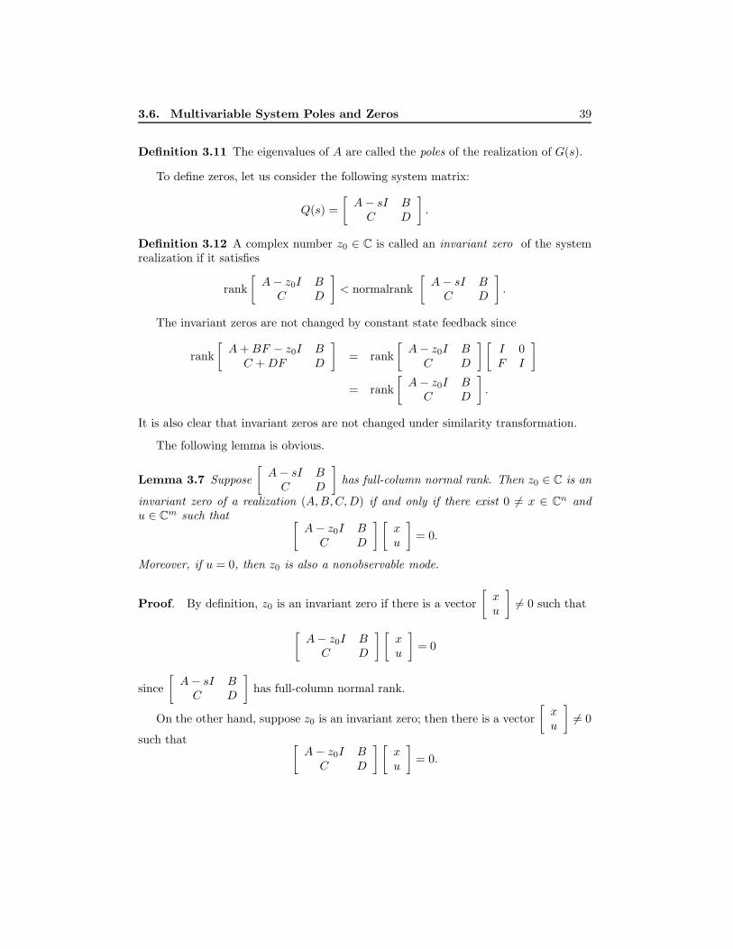
Definition 3.11 The eigenvalues of A are called the poles of the realization of G(s).
To define zeros, let us consider the following system matrix:
Q(s) =[A− sI BC D
].
Definition 3.12 A complex number z0 ∈ C is called an invariant zero of the systemrealization if it satisfies
rank[A− z0I B
C D
]< normalrank
[A− sI BC D
].
The invariant zeros are not changed by constant state feedback since
rank[A+BF − z0I BC +DF D
]= rank
[A− z0I BC D
][I 0F I
]= rank
[A− z0I BC D
].
It is also clear that invariant zeros are not changed under similarity transformation.
The following lemma is obvious.
Lemma 3.7 Suppose[A− sI BC D
]has full-column normal rank. Then z0 ∈ C is an
invariant zero of a realization (A,B,C,D) if and only if there exist 0 6= x ∈ Cn andu ∈ Cm such that [
A− z0I BC D
] [xu
]= 0.
Moreover, if u = 0, then z0 is also a nonobservable mode.
Proof. By definition, z0 is an invariant zero if there is a vector[xu
]6= 0 such that
[A− z0I BC D
][xu
]= 0
since[A− sI BC D
]has full-column normal rank.
On the other hand, suppose z0 is an invariant zero; then there is a vector[xu
]6= 0
such that [A− z0I B
C D
] [xu
]= 0.

40 LINEAR SYSTEMS
We claim that x 6= 0. Otherwise,[BD
]u = 0 or u = 0 since
[A− sI BC D
]has
full-column normal rank (i.e.,[xu
]= 0), which is a contradiction.
Finally, note that if u = 0, then[A− z0I
C
]x = 0
and z0 is a nonobservable mode by PBH test. 2
When the system is square, the invariant zeros can be computed by solving a gen-eralized eigenvalue problem:[
A BC D
]︸ ︷︷ ︸
M
[xu
]= z0
[I 00 0
]︸ ︷︷ ︸
N
[xu
]
using a Matlab command: eig(M, N).
Lemma 3.8 Suppose[A− sI BC D
]has full-row normal rank. Then z0 ∈ C is an
invariant zero of a realization (A,B,C,D) if and only if there exist 0 6= y ∈ Cn andv ∈ Cp such that [
y∗ v∗] [ A− z0I B
C D
]= 0.
Moreover, if v = 0, then z0 is also a noncontrollable mode.
Lemma 3.9 G(s) has full-column (row) normal rank if and only if[A− sI BC D
]has
full-column (row) normal rank.
Proof. This follows by noting that[A− sI BC D
]=[
I 0C(A − sI)−1 I
] [A− sI B
0 G(s)
]and
normalrank[A− sI BC D
]= n+ normalrank(G(s)).
2
Lemma 3.10 Let G(s) ∈ Rp(s) be a p ×m transfer matrix and let (A,B,C,D) be aminimal realization. If the system input is of the form u(t) = u0e
λt, where λ ∈ C is nota pole of G(s) and u0 ∈ Cm is an arbitrary constant vector, then the output due to theinput u(t) and the initial state x(0) = (λI − A)−1Bu0 is y(t) = G(λ)u0e
λt, ∀t ≥ 0. Inparticular, if λ is a zero of G(s), then y(t) = 0.

3.7. Notes and References 41
Proof. The system response with respect to the input u(t) = u0eλt and the initial
condition x(0) = (λI −A)−1Bu0 is (in terms of the Laplace transform)
Y (s) = C(sI −A)−1x(0) + C(sI −A)−1BU(s) +DU(s)= C(sI −A)−1x(0) + C(sI −A)−1Bu0(s− λ)−1 +Du0(s− λ)−1
= C(sI −A)−1x(0) + C[(sI −A)−1 − (λI −A)−1
]Bu0(s− λ)−1
+C(λI −A)−1Bu0(s− λ)−1 +Du0(s− λ)−1
= C(sI −A)−1(x(0)− (λI −A)−1Bu0) +G(λ)u0(s− λ)−1
= G(λ)u0(s− λ)−1.
Hence y(t) = G(λ)u0eλt. 2
Example 3.3 Let
G(s) =[A BC D
]=
−1 −2 1 1 2 30 2 −1 3 2 1−4 −3 −2 1 1 11 1 1 0 0 02 3 4 0 0 0
.Then the invariant zeros of the system can be found using the Matlab command
G=pck(A, B, C, D), z0 = szeros(G), % or
z0 = tzero(A,B,C,D)
which gives z0 = 0.2. Since G(s) is full-row rank, we can find y and v such that[y∗ v∗
] [ A− z0I BC D
]= 0,
which can again be computed using a Matlab command:
null([A− z0 ∗ eye(3),B; C,D]′) =⇒[yv
]=
0.04660.0466−0.1866−0.97020.1399
.
Related MATLAB Commands: spoles, rifd
3.7 Notes and References
Readers are referred to Brogan [1991], Chen [1984], Kailath [1980], and Wonham [1985]for extensive treatment of standard linear system theory.

42 LINEAR SYSTEMS
3.8 Problems
Problem 3.1 Let A ∈ Cn×n and B ∈ Cm×m. Show that X(t) = eAtX(0)eBt is thesolution to
X = AX +XB.
Problem 3.2 Given the impulse response, h1(t), of a linear time-invariant system withmodel
y + a1y + a2y = u
find the impulse response, h(t), of the system
y + a1y + a2y = b0u+ b1u+ b2u.
Justify your answer and generalize your result to nth order systems.
Problem 3.3 Suppose a second order system is given by x = Ax. Suppose it is known
that x(1) =[
4−2
]for x(0) =
[11
]and x(1) =
[5−2
]for x(0) =
[12
]. Find x(n)
for x(0) =[
10
]. Can you determine A?
Problem 3.4 Assume (A,B) is controllable. Show that (F,G) with
F =[A 0C 0
], G =
[B0
]is controllable if and only if [
A BC 0
]is a full-row rank matrix.
Problem 3.5 Let λi, i = 1, 2, . . . , n be n distinct eigenvalues of a matrix A ∈ Cn×n andlet xi and yi be the corresponding right- and left-unit eigenvectors such that y∗i xi = 1.Show that
y∗i xj = δij , A =n∑i=1
λixiy∗i
and
C(sI −A)−1B =n∑i=1
(Cxi)(y∗iB)s− λi
.
Furthermore, show that the mode λi is controllable iff y∗iB 6= 0 and the mode λi isobservable iff Cxi 6= 0.

3.8. Problems 43
Problem 3.6 Let (A, b, c) be a realization with A ∈ Rn×n, b ∈ Rn, and c∗ ∈ Rn.Assume that λi(A) + λj(A) 6= 0 for all i, j. This assumption ensures the existence ofX ∈ Rn×n such that
AX +XA+ bc = 0
Show that X is nonsingular if and only if (A, b) is controllable and (c, A) is observable.
Problem 3.7 Compute the system zeros and the corresponding zero directions of thefollowing transfer functions
G1(s) =
1 2 2 21 0 3 40 1 1 21 0 2 0
, G2(s) =
−1 −2 1 20 1 2 11 1 0 01 1 0 0
,
G3(s) =[
2(s+ 1)(s+ 2)s(s+ 3)(s+ 4)
s+ 2(s+ 1)(s+ 3)
], G4(s) =
1
s+ 1s+ 3
(s+ 1)(s− 2)
10s− 2
5s+ 3
Also find the vectors x and u whenever appropriate so that either[
A− zI BC D
] [xu
]= 0 or
[x∗ u∗
] [ A− zI BC D
]= 0.

44 LINEAR SYSTEMS

Chapter 4
H2 and H∞ Spaces
The most important objective of a control system is to achieve certain performancespecifications in addition to providing internal stability. One way to describe the per-formance specifications of a control system is in terms of the size of certain signals ofinterest. For example, the performance of a tracking system could be measured by thesize of the tracking error signal. In this chapter, we look at several ways of defining asignal’s size (i.e., at several norms for signals). Of course, which norm is most appro-priate depends on the situation at hand. For that purpose, we shall first introduce theHardy spaces H2 and H∞. Some state-space methods of computing real rational H2
and H∞ transfer matrix norms are also presented.
4.1 Hilbert Spaces
Recall the inner product of vectors defined on a Euclidean space Cn:
〈x, y〉 := x∗y =n∑i=1
xiyi ∀x =
x1
...xn
, y =
y1
...yn
∈ Cn.Note that many important metric notions and geometrical properties, such as length,distance, angle, and the energy of physical systems, can be deduced from this innerproduct. For instance, the length of a vector x ∈ Cn is defined as
‖x‖ :=√〈x, x〉
and the angle between two vectors x, y ∈ Cn can be computed from
cos∠(x, y) =〈x, y〉‖x‖ ‖y‖ , ∠(x, y) ∈ [0, π].
The two vectors are said to be orthogonal if ∠(x, y) = π2 .
45

46 H2 AND H∞ SPACES
We now consider a natural generalization of the inner product on Cn to more general(possibly infinite dimensional) vector spaces.
Definition 4.1 Let V be a vector space over C. An inner product1 on V is a complex-valued function,
〈·, ·〉 : V × V 7−→ Csuch that for any x, y, z ∈ V and α, β ∈ C
(i) 〈x, αy + βz〉 = α〈x, y〉 + β〈x, z〉
(ii) 〈x, y〉 = 〈y, x〉
(iii) 〈x, x〉 > 0 if x 6= 0.
A vector space V with an inner product is called an inner product space.
It is clear that the inner product defined above induces a norm ‖x‖ :=√〈x, x〉, so
that the norm conditions in Chapter 2 are satisfied. In particular, the distance betweenvectors x and y is d(x, y) = ‖x− y‖.
Two vectors x and y in an inner product space V are said to be orthogonal if〈x, y〉 = 0, denoted x ⊥ y. More generally, a vector x is said to be orthogonal to a setS ⊂ V , denoted by x ⊥ S, if x ⊥ y for all y ∈ S.
The inner product and the inner product induced norm have the following familiarproperties.
Theorem 4.1 Let V be an inner product space and let x, y ∈ V . Then
(i) |〈x, y〉| ≤ ‖x‖ ‖y‖ (Cauchy-Schwarz inequality). Moreover, the equality holds ifand only if x = αy for some constant α or y = 0.
(ii) ‖x+ y‖2 + ‖x− y‖2 = 2 ‖x‖2 + 2 ‖y‖2 (Parallelogram law).
(iii) ‖x+ y‖2 = ‖x‖2 + ‖y‖2 if x ⊥ y.
A Hilbert space is a complete inner product space with the norm induced by its innerproduct. For example, Cn with the usual inner product is a (finite dimensional) Hilbertspace. More generally, it is straightforward to verify that Cn×m with the inner productdefined as
〈A,B〉 := traceA∗B =n∑i=1
m∑j=1
aijbij ∀A,B ∈ Cn×m
is also a (finite dimensional) Hilbert space.A well-know infinite dimensional Hilbert space is L2[a, b], which consists of all square
integrable and Lebesgue measurable functions defined on an interval [a, b] with the innerproduct defined as
〈f, g〉 :=∫ b
a
f(t)∗g(t)dt
1The property (i) in the following list is the other way around to the usual mathematical conventionsince we want to have 〈x, y〉 = x∗y rather than y∗x for x, y ∈ Cn.

4.2. H2 and H∞ Spaces 47
for f, g ∈ L2[a, b]. Similarly, if the functions are vector or matrix-valued, the innerproduct is defined correspondingly as
〈f, g〉 :=∫ b
a
trace [f(t)∗g(t)] dt.
Some spaces used often in this book are L2[0,∞),L2(−∞, 0],L2(−∞,∞). More pre-cisely, they are defined asL2 = L2(−∞,∞): Hilbert space of matrix-valued functions on R, with inner product
〈f, g〉 :=∫ ∞−∞
trace [f(t)∗g(t)] dt.
L2+ = L2[0,∞): subspace of L2(−∞,∞) with functions zero for t < 0.
L2− = L2(−∞, 0]: subspace of L2(−∞,∞) with functions zero for t > 0.
4.2 H2 and H∞ Spaces
Let S ⊂ C be an open set, and let f(s) be a complex-valued function defined on S:
f(s) : S 7−→ C.
Then f(s) is said to be analytic at a point z0 in S if it is differentiable at z0 and alsoat each point in some neighborhood of z0. It is a fact that if f(s) is analytic at z0 thenf has continuous derivatives of all orders at z0. Hence, a function analytic at z0 hasa power series representation at z0. The converse is also true (i.e., if a function hasa power series at z0, then it is analytic at z0). A function f(s) is said to be analyticin S if it has a derivative or is analytic at each point of S. A matrix-valued functionis analytic in S if every element of the matrix is analytic in S. For example, all realrational stable transfer matrices are analytic in the right-half plane and e−s is analyticeverywhere.
A well-know property of the analytic functions is the so-called maximum modulustheorem.
Theorem 4.2 If f(s) is defined and continuous on a closed-bounded set S and analyticon the interior of S, then |f(s)| cannot attain the maximum in the interior of S unlessf(s) is a constant.
The theorem implies that |f(s)| can only achieve its maximum on the boundary of S;that is,
maxs∈S|f(s)| = max
s∈∂S|f(s)|
where ∂S denotes the boundary of S. Next we consider some frequently used complex(matrix) function spaces.

48 H2 AND H∞ SPACES
L2(jR) Space
L2(jR) or simply L2 is a Hilbert space of matrix-valued (or scalar-valued) func-tions on jR and consists of all complex matrix functions F such that the followingintegral is bounded: ∫ ∞
−∞trace [F ∗(jω)F (jω)] dω <∞.
The inner product for this Hilbert space is defined as
〈F,G〉 :=1
2π
∫ ∞−∞
trace [F ∗(jω)G(jω)] dω
for F,G ∈ L2, and the inner product induced norm is given by
‖F‖2 :=√〈F, F 〉.
For example, all real rational strictly proper transfer matrices with no poles on theimaginary axis form a subspace (not closed) of L2(jR) that is denoted by RL2(jR) orsimply RL2.
H2 Space2
H2 is a (closed) subspace of L2(jR) with matrix functions F (s) analytic inRe(s) > 0 (open right-half plane). The corresponding norm is defined as
‖F‖22 := supσ>0
1
2π
∫ ∞−∞
trace [F ∗(σ + jω)F (σ + jω)]dω.
It can be shown3 that
‖F‖22 =1
2π
∫ ∞−∞
trace [F ∗(jω)F (jω)] dω.
Hence, we can compute the norm for H2 just as we do for L2. The real rationalsubspace ofH2, which consists of all strictly proper and real rational stable transfermatrices, is denoted by RH2.
H⊥2 Space
H⊥2 is the orthogonal complement of H2 in L2; that is, the (closed) subspace offunctions in L2 that are analytic in the open left-half plane. The real rationalsubspace of H⊥2 , which consists of all strictly proper rational transfer matriceswith all poles in the open right-half plane, will be denoted by RH⊥2 . It is easy tosee that if G is a strictly proper, stable, and real rational transfer matrix, thenG ∈ H2 and G∼ ∈ H⊥2 . Most of our study in this book will be focused on the realrational case.
2The H2 space and H∞ space defined in this subsection together with the Hp spaces, p ≥ 1,which will not be introduced in this book, are usually called Hardy spaces and are named after themathematician G. H. Hardy (hence the notation of H).
3See Francis [1987].
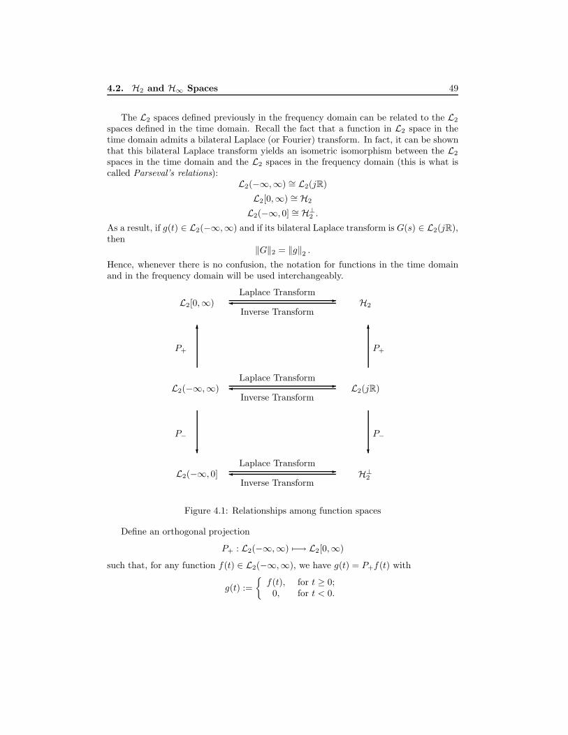
4.2. H2 and H∞ Spaces 49
The L2 spaces defined previously in the frequency domain can be related to the L2
spaces defined in the time domain. Recall the fact that a function in L2 space in thetime domain admits a bilateral Laplace (or Fourier) transform. In fact, it can be shownthat this bilateral Laplace transform yields an isometric isomorphism between the L2
spaces in the time domain and the L2 spaces in the frequency domain (this is what iscalled Parseval’s relations):
L2(−∞,∞) ∼= L2(jR)
L2[0,∞) ∼= H2
L2(−∞, 0] ∼= H⊥2 .As a result, if g(t) ∈ L2(−∞,∞) and if its bilateral Laplace transform is G(s) ∈ L2(jR),then
‖G‖2 = ‖g‖2 .Hence, whenever there is no confusion, the notation for functions in the time domainand in the frequency domain will be used interchangeably.
H2
L2(jR)
H⊥2L2(−∞, 0]
L2(−∞,∞)
L2[0,∞)
P−
P+
Laplace Transform
Inverse Transform
Inverse Transform
Laplace Transform
Inverse Transform
Laplace Transform
P−
P+
? ?
66
-
-
-
Figure 4.1: Relationships among function spaces
Define an orthogonal projection
P+ : L2(−∞,∞) 7−→ L2[0,∞)
such that, for any function f(t) ∈ L2(−∞,∞), we have g(t) = P+f(t) with
g(t) :=f(t), for t ≥ 0;
0, for t < 0.

50 H2 AND H∞ SPACES
In this book, P+ will also be used to denote the projection from L2(jR) onto H2.Similarly, define P− as another orthogonal projection from L2(−∞,∞) onto L2(−∞, 0](or L2(jR) onto H⊥2 ). Then the relationships between L2 spaces and H2 spaces can beshown as in Figure 4.1.
Other classes of important complex matrix functions used in this book are thosebounded on the imaginary axis.
L∞(jR) Space
L∞(jR) or simply L∞ is a Banach space of matrix-valued (or scalar-valued) func-tions that are (essentially) bounded on jR, with norm
‖F‖∞ := ess supω∈R
σ [F (jω)] .
The rational subspace of L∞, denoted by RL∞(jR) or simply RL∞, consists ofall proper and real rational transfer matrices with no poles on the imaginary axis.
H∞ Space
H∞ is a (closed) subspace of L∞ with functions that are analytic and bounded inthe open right-half plane. The H∞ norm is defined as
‖F‖∞ := supRe(s)>0
σ [F (s)] = supω∈R
σ [F (jω)] .
The second equality can be regarded as a generalization of the maximum modulustheorem for matrix functions. (See Boyd and Desoer [1985] for a proof.) The realrational subspace of H∞ is denoted by RH∞, which consists of all proper and realrational stable transfer matrices.
H−∞ Space
H−∞ is a (closed) subspace of L∞ with functions that are analytic and bounded inthe open left-half plane. The H−∞ norm is defined as
‖F‖∞ := supRe(s)<0
σ [F (s)] = supω∈R
σ [F (jω)] .
The real rational subspace ofH−∞ is denoted byRH−∞, which consists of all proper,real rational, antistable transfer matrices (i.e., functions with all poles in the openright-half plane).
Let G(s) ∈ L∞ be a p× q transfer matrix. Then a multiplication operator is defined as
MG : L2 7−→ L2
MGf := Gf.

4.2. H2 and H∞ Spaces 51
In writing the preceding mapping, we have assumed that f has a compatible dimension.A more accurate description of the foregoing operator should be
MG : Lq2 7−→ Lp2.
That is, f is a q-dimensional vector function with each component in L2. However, weshall suppress all dimensions in this book and assume that all objects have compatibledimensions.
A useful fact about the multiplication operator is that the norm of a matrix G inL∞ equals the norm of the corresponding multiplication operator.
Theorem 4.3 Let G ∈ L∞ be a p× q transfer matrix. Then ‖MG‖ = ‖G‖∞.
Remark 4.1 It is also true that this operator norm equals the norm of the operatorrestricted to H2 (or H⊥2 ); that is,
‖MG‖ = ‖MG|H2‖ := sup ‖Gf‖2 : f ∈ H2, ‖f‖2 ≤ 1 .
This will be clear in the proof where an f ∈ H2 is constructed. 3
Proof. By definition, we have
‖MG‖ = sup ‖Gf‖2 : f ∈ L2, ‖f‖2 ≤ 1 .
First we see that ‖G‖∞ is an upper bound for the operator norm:
‖Gf‖22 =1
2π
∫ ∞−∞
f∗(jω)G∗(jω)G(jω)f(jω) dω
≤ ‖G‖2∞1
2π
∫ ∞−∞‖f(jω)‖2 dω
= ‖G‖2∞‖f‖22.
To show that ‖G‖∞ is the least upper bound, first choose a frequency ω0 where σ [G(jω)]is maximum; that is,
σ [G(jω0)] = ‖G‖∞,and denote the singular value decomposition of G(jω0) by
G(jω0) = σu1(jω0)v∗1(jω0) +r∑i=2
σiui(jω0)v∗i (jω0)
where r is the rank of G(jω0) and ui, vi have unit length.Next we assume that G(s) has real coefficients and we shall construct a function
f(s) ∈ H2 with real coefficients so that the norm is approximately achieved. [It willbe clear in the following that the proof is much simpler if f is allowed to have complexcoefficients, which is necessary when G(s) has complex coefficients.]

52 H2 AND H∞ SPACES
If ω0 <∞, write v1(jω0) as
v1(jω0) =
α1e
jθ1
α2ejθ2
...αqe
jθq
where αi ∈ R is such that θi ∈ (−π, 0] and q is the column dimension of G. Now let0 ≤ βi ≤ ∞ be such that
θi = ∠(βi − jω0
βi + jω0
)(with βi →∞ if θi = 0) and let f be given by
f(s) =
α1
β1−sβ1+s
α2β2−sβ2+s...
αqβq−sβq+s
f(s)
(with 1 replacing βi−sβi+s
if θi = 0), where a scalar function f is chosen so that
|f(jω)| =c if |ω − ω0| < ε or |ω + ω0| < ε0 otherwise
where ε is a small positive number and c is chosen so that f has unit 2-norm (i.e.,c =
√π/2ε). This, in turn, implies that f has unit 2-norm. Then
‖Gf‖22 ≈ 12π
[σ [G(−jω0)]2 π + σ [G(jω0)]2 π
]= σ [G(jω0)]2 = ‖G‖2∞.
Similarly, if ω0 =∞, the conclusion follows by letting ω0 →∞ in the foregoing. 2
Illustrative MATLAB Commands:
[sv, w]=sigma(A, B, C, D); % frequency response of the singular values; or
w=logspace(l, h, n); sv=sigma(A, B, C, D, w); % n points between 10l and10h.
Related MATLAB Commands: semilogx, semilogy, bode, freqs, nichols, frsp,vsvd, vplot, pkvnorm

4.3. Computing L2 and H2 Norms 53
4.3 Computing L2 and H2 Norms
Let G(s) ∈ L2 and recall that the L2 norm of G is defined as
‖G‖2 :=
√1
2π
∫ ∞−∞
traceG∗(jω)G(jω) dω
= ‖g‖2
=
√∫ ∞−∞
traceg∗(t)g(t) dt
where g(t) denotes the convolution kernel of G.It is easy to see that the L2 norm defined previously is finite iff the transfer matrix G
is strictly proper; that is, G(∞) = 0. Hence, we will generally assume that the transfermatrix is strictly proper whenever we refer to the L2 norm of G (of course, this alsoapplies to H2 norms). One straightforward way of computing the L2 norm is to usecontour integral. Suppose G is strictly proper; then we have
‖G‖22 =1
2π
∫ ∞−∞
traceG∗(jω)G(jω) dω
=1
2πj
∮traceG∼(s)G(s) ds.
The last integral is a contour integral along the imaginary axis and around an infinitesemicircle in the left-half plane; the contribution to the integral from this semicircleequals zero because G is strictly proper. By the residue theorem, ‖G‖22 equals the sumof the residues of traceG∼(s)G(s) at its poles in the left-half plane.
Although ‖G‖2 can, in principle, be computed from its definition or from the methodjust suggested, it is useful in many applications to have alternative characterizations andto take advantage of the state-space representations of G. The computation of a RH2
transfer matrix norm is particularly simple.
Lemma 4.4 Consider a transfer matrix
G(s) =[A BC 0
]with A stable. Then we have
‖G‖22 = trace(B∗QB) = trace(CPC∗) (4.1)
where Q and P are observability and controllability Gramians that can be obtained fromthe following Lyapunov equations:
AP + PA∗ +BB∗ = 0 A∗Q+QA+ C∗C = 0.

54 H2 AND H∞ SPACES
Proof. Since G is stable, we have
g(t) = L−1(G) =CeAtB, t ≥ 00, t < 0
and
‖G‖22 =∫ ∞
0
traceg∗(t)g(t) dt =∫ ∞
0
traceg(t)g(t)∗ dt
=∫ ∞
0
traceB∗eA∗tC∗CeAtB dt =∫ ∞
0
traceCeAtBB∗eA∗tC∗ dt.
The lemma follows from the fact that the controllability Gramian of (A,B) and theobservability Gramian of (C,A) can be represented as
Q =∫ ∞
0
eA∗tC∗CeAt dt, P =
∫ ∞0
eAtBB∗eA∗t dt,
which can also be obtained from
AP + PA∗ +BB∗ = 0 A∗Q+QA+ C∗C = 0.
2
To compute the L2 norm of a rational transfer function, G(s) ∈ RL2, using thestate-space approach, let G(s) = [G(s)]+ + [G(s)]− with G+ ∈ RH2 and G− ∈ RH⊥2 ;then
‖G‖22 = ‖[G(s)]+‖22 + ‖[G(s)]−‖22where ‖[G(s)]+‖2 and ‖[G(s)]−‖2 = ‖[G(−s)]+‖2 = ‖([G(s)]−)∼‖2 can be computedusing the preceding lemma.
Still another useful characterization of the H2 norm of G is in terms of hypotheticalinput-output experiments. Let ei denote the ith standard basis vector of Rm, where mis the input dimension of the system. Apply the impulsive input δ(t)ei [δ(t) is the unitimpulse] and denote the output by zi(t)(= g(t)ei). Assume D = 0; then zi ∈ L2+ and
‖G‖22 =m∑i=1
‖zi‖22.
Note that this characterization of the H2 norm can be appropriately generalized fornonlinear time-varying systems; see Chen and Francis [1992] for an application of thisnorm in sampled-data control.
Example 4.1 Consider a transfer matrix
G =
3(s+ 3)
(s− 1)(s+ 2)2
s− 1s+ 1
(s+ 2)(s+ 3)1
s− 4
= Gs +Gu

4.4. Computing L∞ and H∞ Norms 55
with
Gs =
−2 0 −1 00 −3 2 01 0 0 01 1 0 0
, Gu =
1 0 4 20 4 0 11 0 0 00 1 0 0
.Then the command h2norm(Gs) gives ‖Gs‖2 = 0.6055 and h2norm(cjt(Gu)) gives
‖Gu‖2 = 3.182. Hence ‖G‖2 =√‖Gs‖22 + ‖Gu‖22 = 3.2393.
Illustrative MATLAB Commands:
P = gram(A,B); Q = gram(A′,C′); or P = lyap(A,B ∗B′);
[Gs,Gu] = sdecomp(G); % decompose into stable and antistable parts.
4.4 Computing L∞ and H∞ Norms
We shall first consider, as in the L2 case, how to compute the ∞ norm of an RL∞transfer matrix. Let G(s) ∈ RL∞ and recall that the L∞ norm of a matrix rationaltransfer function G is defined as
‖G‖∞ := supωσG(jω).
The computation of the L∞ norm of G is complicated and requires a search. A controlengineering interpretation of the infinity norm of a scalar transfer function G is thedistance in the complex plane from the origin to the farthest point on the Nyquist plotof G, and it also appears as the peak value on the Bode magnitude plot of |G(jω)|.Hence the ∞ norm of a transfer function can, in principle, be obtained graphically.
To get an estimate, set up a fine grid of frequency points:
ω1, · · · , ωN.
Then an estimate for ‖G‖∞ is
max1≤k≤N
σG(jωk).
This value is usually read directly from a Bode singular value plot. The RL∞ norm canalso be computed in state-space.
Lemma 4.5 Let γ > 0 and
G(s) =[A BC D
]∈ RL∞. (4.2)

56 H2 AND H∞ SPACES
Then ‖G‖∞ < γ if and only if σ(D) < γ and the Hamiltonian matrix H has no eigen-values on the imaginary axis where
H :=[
A+BR−1D∗C BR−1B∗
−C∗(I +DR−1D∗)C −(A+BR−1D∗C)∗
](4.3)
and R = γ2I −D∗D.
Proof. Let Φ(s) = γ2I − G∼(s)G(s). Then it is clear that ‖G‖∞ < γ if and only ifΦ(jω) > 0 for all ω ∈ R. Since Φ(∞) = R > 0 and since Φ(jω) is a continuous functionof ω, Φ(jω) > 0 for all ω ∈ R if and only if Φ(jω) is nonsingular for all ω ∈ R ∪ ∞;that is, Φ(s) has no imaginary axis zero. Equivalently, Φ−1(s) has no imaginary axispole. It is easy to compute by some simple algebra that
Φ−1(s) =
H
[BR−1
−C∗DR−1
][R−1D∗C R−1B∗
]R−1
.Thus the conclusion follows if the above realization has neither uncontrollable modesnor unobservable modes on the imaginary axis. Assume that jω0 is an eigenvalueof H but not a pole of Φ−1(s). Then jω0 must be either an unobservable mode of
([R−1D∗C R−1B∗
],H) or an uncontrollable mode of (H,
[BR−1
−C∗DR−1
]). Now
suppose jω0 is an unobservable mode of ([R−1D∗C R−1B∗
],H). Then there exists
an x0 =[x1
x2
]6= 0 such that
Hx0 = jω0x0,[R−1D∗C R−1B∗
]x0 = 0.
These equations can be simplified to
(jω0I −A)x1 = 0(jω0I +A∗)x2 = −C∗Cx1
D∗Cx1 +B∗x2 = 0.
Since A has no imaginary axis eigenvalues, we have x1 = 0 and x2 = 0. This contradictsour assumption, and hence the realization has no unobservable modes on the imaginaryaxis.
Similarly, a contradiction will also be arrived at if jω0 is assumed to be an uncon-
trollable mode of (H,[
BR−1
−C∗DR−1
]). 2

4.4. Computing L∞ and H∞ Norms 57
Bisection Algorithm
Lemma 4.5 suggests the following bisection algorithm to compute RL∞ norm:
(a) Select an upper bound γu and a lower bound γl such that γl ≤ ‖G‖∞ ≤ γu;
(b) If (γu− γl)/γl ≤specified level, stop; ‖G‖ ≈ (γu + γl)/2. Otherwise go to the nextstep;
(c) Set γ = (γl + γu)/2;
(d) Test if ‖G‖∞ < γ by calculating the eigenvalues of H for the given γ;
(e) If H has an eigenvalue on jR, set γl = γ; otherwise set γu = γ; go back to step(b).
Of course, the above algorithm applies to H∞ norm computation as well. Thus L∞norm computation requires a search, over either γ or ω, in contrast to L2 (H2) normcomputation, which does not. A somewhat analogous situation occurs for constantmatrices with the norms ‖M‖22 = trace(M∗M) and ‖M‖∞ = σ[M ]. In principle, ‖M‖22can be computed exactly with a finite number of operations, as can the test for whetherσ(M) < γ (e.g., γ2I −M∗M > 0), but the value of σ(M) cannot. To compute σ(M),we must use some type of iterative algorithm.
Remark 4.2 It is clear that ‖G‖∞ < γ iff∥∥γ−1G
∥∥∞ < 1. Hence, there is no loss of
generality in assuming γ = 1. This assumption will often be made in the remainder ofthis book. It is also noted that there are other fast algorithms to carry out the precedingnorm computation; nevertheless, this bisection algorithm is the simplest. 3
Additional interpretations can be given for the H∞ norm of a stable matrix transferfunction. When G(s) is a single-input and single-output system, the H∞ norm of theG(s) can be regarded as the largest possible amplification factor of the system’s steady-state response to sinusoidal excitations. For example, the steady-state response of thesystem with respect to a sinusoidal input u(t) = U sin(ω0t+ φ) is
y(t) = U |G(jω0)| sin (ω0t+ φ+ ∠G(jω0))
and thus the maximum possible amplification factor is supω0
|G(jω0)|, which is precisely
the H∞ norm of the transfer function.In the multiple-input and multiple-output case, the H∞ norm of a transfer matrix
G ∈ RH∞ can also be regarded as the largest possible amplification factor of thesystem’s steady-state response to sinusoidal excitations in the following sense: Let thesinusoidal inputs be
u(t) =
u1 sin(ω0t+ φ1)u2 sin(ω0t+ φ2)
...uq sin(ω0t+ φq)
, u =
u1
u2
...uq
.

58 H2 AND H∞ SPACES
Then the steady-state response of the system can be written as
y(t) =
y1 sin(ω0t+ θ1)y2 sin(ω0t+ θ2)
...yp sin(ω0t+ θp)
, y =
y1
y2
...yp
for some yi, θi, i = 1, 2, . . . , p, and furthermore,
‖G‖∞ = supφi,ωo,u
‖y‖‖u‖
where ‖·‖ is the Euclidean norm. The details are left as an exercise.
Example 4.2 Consider a mass/spring/damper system as shown in Figure 4.2.
F
F
m
m
k b
bk
x
x
2 2
2
11
1
1
2
1
2
Figure 4.2: A two-mass/spring/damper system
The dynamical system can be described by the following differential equations:x1
x2
x3
x4
= A
x1
x2
x3
x4
+B
[F1
F2
]

4.4. Computing L∞ and H∞ Norms 59
10−1
100
101
10−2
10−1
100
101
102
The largest singular value
The smallest singular value
frequency (rad/sec)
Figure 4.3: ‖G‖∞ is the peak of the largest singular value of G(jω)
with
A =
0 0 1 00 0 0 1
− k1
m1
k1
m1− b1m1
b1m1
k1
m2−k1 + k2
m2
b1m2
−b1 + b2m2
, B =
0 00 01m1
0
01m2
.
Suppose that G(s) is the transfer matrix from (F1, F2) to (x1, x2); that is,
C =[
1 0 0 00 1 0 0
], D = 0,
and suppose k1 = 1, k2 = 4, b1 = 0.2, b2 = 0.1, m1 = 1, and m2 = 2 with appropriateunits. The following Matlab commands generate the singular value Bode plot of theabove system as shown in Figure 4.3.
G=pck(A,B,C,D);
hinfnorm(G,0.0001) or linfnorm(G,0.0001) % relative error ≤ 0.0001
w=logspace(-1,1,200); % 200 points between 1 = 10−1 and 10 = 101;
Gf=frsp(G,w); % computing frequency response;
[u,s,v]=vsvd(Gf); % SVD at each frequency;

60 H2 AND H∞ SPACES
vplot(′liv, lm′, s), grid % plot both singular values and grid.
Then the H∞ norm of this transfer matrix is ‖G(s)‖∞ = 11.47, which is shown asthe peak of the largest singular value Bode plot in Figure 4.3. Since the peak is achievedat ωmax = 0.8483, exciting the system using the following sinusoidal input[
F1
F2
]=[
0.9614 sin(0.8483t)0.2753 sin(0.8483t− 0.12)
]gives the steady-state response of the system as[
x1
x2
]=[
11.47× 0.9614 sin(0.8483t− 1.5483)11.47× 0.2753 sin(0.8483t− 1.4283)
].
This shows that the system response will be amplified 11.47 times for an input signalat the frequency ωmax, which could be undesirable if F1 and F2 are disturbance forceand x1 and x2 are the positions to be kept steady.
Example 4.3 Consider a two-by-two transfer matrix
G(s) =
10(s+ 1)
s2 + 0.2s+ 1001
s+ 1s+ 2
s2 + 0.1s+ 105(s+ 1)
(s+ 2)(s+ 3)
.A state-space realization of G can be obtained using the following Matlab commands:
G11=nd2sys([10,10],[1,0.2,100]);
G12=nd2sys(1,[1,1]);
G21=nd2sys([1,2],[1,0.1,10]);
G22=nd2sys([5,5],[1,5,6]);
G=sbs(abv(G11,G21),abv(G12,G22));
Next, we set up a frequency grid to compute the frequency response of G and thesingular values of G(jω) over a suitable range of frequency.
w=logspace(0,2,200); % 200 points between 1 = 100 and 100 = 102;
Gf=frsp(G,w); % computing frequency response;
[u,s,v]=vsvd(Gf); % SVD at each frequency;

4.5. Notes and References 61
vplot(′liv, lm′, s), grid % plot both singular values and grid;
pkvnorm(s) % find the norm from the frequency response of the singular values.
The singular values of G(jω) are plotted in Figure 4.4, which gives an estimate of‖G‖∞ ≈ 32.861. The state-space bisection algorithm described previously leads to‖G‖∞ = 50.25± 0.01 and the corresponding Matlab command is
hinfnorm(G,0.0001) or linfnorm(G,0.0001) % relative error ≤ 0.0001.
100
101
102
10−2
10−1
100
101
102
Figure 4.4: The largest and the smallest singular values of G(jω)
The preceding computational results show clearly that the graphical method can leadto a wrong answer for a lightly damped system if the frequency grid is not sufficientlydense. Indeed, we would get ‖G‖∞ ≈ 43.525, 48.286 and 49.737 from the graphicalmethod if 400, 800, and 1600 frequency points are used, respectively.
Related MATLAB Commands: linfnorm, vnorm, getiv, scliv, var2con, xtract,xtracti
4.5 Notes and References
The basic concept of function spaces presented in this chapter can be found in anystandard functional analysis textbook, for instance, Naylor and Sell [1982] and Gohbergand Goldberg [1981]. The system theoretical interpretations of the norms and function

62 H2 AND H∞ SPACES
spaces can be found in Desoer and Vidyasagar [1975]. The bisection L∞ norm compu-tational algorithm was first developed in Boyd, Balakrishnan, and Kabamba [1989]. Amore efficient L∞ norm computational algorithm is presented in Bruinsma and Stein-buch [1990].
4.6 Problems
Problem 4.1 Let G(s) be a matrix in RH∞. Prove that∥∥∥∥[ GI
]∥∥∥∥2
∞= ‖G‖2∞ + 1.
Problem 4.2 (Parseval relation) Let f(t), g(t) ∈ L2, F (jω) = Ff(t), and G(jω) =Fg(t). Show that ∫ ∞
−∞f(t)g(t)dt =
12π
∫ ∞−∞
F (jω)G∗(jω)dω
and ∫ ∞−∞|f(t)|2dt =
12π
∫ ∞−∞|F (jω)|2dω.
Note that
F (jω) =∫ ∞−∞
f(t)e−jωtdt, f(t) = F−1(F (jω)) =1
2π
∫ ∞−∞
F (jω)ejωtdω.
where F−1 denotes the inverse Fourier transform.
Problem 4.3 Suppose A is stable. Show∫ ∞−∞
(jωI −A)−1dω = πI.
Suppose G(s) =[A BC 0
]∈ RH∞ and let Q = Q∗ be the observability Gramian. Use
the above formula to show that
12π
∫ ∞−∞
G∼(jω)G(jω)dω = B∗QB.
[Hint: Use the fact that G∼(s)G(s) = F∼(s) + F (s) and F (s) = B∗Q(sI −A)−1B.]
Problem 4.4 Compute the 2-norm and ∞-norm of the following systems:
G1(s) =
1
s+ 1s+ 3
(s+ 1)(s− 2)
10s− 2
5s+ 3
, G2(s) =
1 0 12 3 11 2 0

4.6. Problems 63
G3(s) =
−1 −2 11 0 02 3 0
, G4(s) =
−1 −2 −3 1 21 0 0 0 10 1 0 2 01 0 0 1 00 1 1 0 2
.Problem 4.5 Let r(t) = sinωt be the input signal to a plant
G(s) =ω2n
s2 + 2ξωns+ ω2n
with 0 < ξ < 1/√
2. Find the steady-state response of the system y(t). Also find thefrequency ω that gives the largest magnitude steady-state response of y(t).
Problem 4.6 Let G(s) ∈ RH∞ be a p× q transfer matrix and y = G(s)u. Suppose
u(t) =
u1 sin(ω0t+ φ1)u2 sin(ω0t+ φ2)
...uq sin(ω0t+ φq)
, u =
u1
u2
...uq
.Show that the steady-state response of the system is given by
y(t) =
y1 sin(ω0t+ θ1)y2 sin(ω0t+ θ2)
...yp sin(ω0t+ θp)
, y =
y1
y2
...yp
for some yi and θi, i = 1, 2, . . . , p. Show that sup
φi,ωo,‖u‖2≤1
‖y‖2 = ‖G‖∞.
Problem 4.7 Write a Matlab program to plot, versus γ, the distance from the imag-inary axis to the nearest eigenvalue of the Hamiltonian matrix for a given state-spacemodel with stable A. Try it on
s+ 1(s+ 2)(s+ 3)
s
s+ 1
s2 − 2(s+ 3)(s+ 4)
s+ 4(s+ 1)(s+ 2)
.Read off the value of the H∞-norm. Compare with the Matlab function hinfnorm.
Problem 4.8 Let G(s) =1
(s2 + 2ξs+ 1)(s+ 1). Compute ‖G(s)‖∞ using the Bode
plot and state-space algorithm, respectively for ξ = 1, 0.1, 0.01, 0.001 and compare theresults.

64 H2 AND H∞ SPACES

Chapter 5
Internal Stability
This chapter introduces the feedback structure and discusses its stability and variousstability tests. The arrangement of this chapter is as follows: Section 5.1 discusses thenecessity for introducing feedback structure and describes the general feedback con-figuration. Section 5.2 defines the well-posedness of the feedback loop. Section 5.3introduces the notion of internal stability and various stability tests. Section 5.4 intro-duces the stable coprime factorizations of rational matrices. The stability conditions interms of various coprime factorizations are also considered in this section.
5.1 Feedback Structure
In designing control systems, there are several fundamental issues that transcend theboundaries of specific applications. Although they may differ for each application andmay have different levels of importance, these issues are generic in their relationship tocontrol design objectives and procedures. Central to these issues is the requirement toprovide satisfactory performance in the face of modeling errors, system variations, anduncertainty. Indeed, this requirement was the original motivation for the developmentof feedback systems. Feedback is only required when system performance cannot beachieved because of uncertainty in system characteristics. A more detailed treatmentof model uncertainties and their representations will be discussed in Chapter 8.
For the moment, assuming we are given a model including a representation of un-certainty that we believe adequately captures the essential features of the plant, thenext step in the controller design process is to determine what structure is necessaryto achieve the desired performance. Prefiltering input signals (or open-loop control)can change the dynamic response of the model set but cannot reduce the effect of un-certainty. If the uncertainty is too great to achieve the desired accuracy of response,then a feedback structure is required. The mere assumption of a feedback structure,however, does not guarantee a reduction of uncertainty, and there are many obstaclesto achieving the uncertainty-reducing benefits of feedback. In particular, since for any
65

66 INTERNAL STABILITY
reasonable model set representing a physical system uncertainty becomes large and thephase is completely unknown at sufficiently high frequencies, the loop gain must besmall at those frequencies to avoid destabilizing the high-frequency system dynamics.Even worse is that the feedback system actually increases uncertainty and sensitivity inthe frequency ranges where uncertainty is significantly large. In other words, becauseof the type of sets required to model physical systems reasonably and because of therestriction that our controllers be causal, we cannot use feedback (or any other controlstructure) to cause our closed-loop model set to be a proper subset of the open-loopmodel set. Often, what can be achieved with intelligent use of feedback is a signifi-cant reduction of uncertainty for certain signals of importance with a small increasespread over other signals. Thus, the feedback design problem centers around the trade-off involved in reducing the overall impact of uncertainty. This tradeoff also occurs, forexample, when using feedback to reduce command/disturbance error while minimizingresponse degradation due to measurement noise. To be of practical value, a designtechnique must provide means for performing these tradeoffs. We shall discuss thesetradeoffs in more detail in the next chapter.
To focus our discussion, we shall consider the standard feedback configuration shownin Figure 5.1. It consists of the interconnected plant P and controller K forced bycommand r, sensor noise n, plant input disturbance di, and plant output disturbanced. In general, all signals are assumed to be multivariable, and all transfer matrices areassumed to have appropriate dimensions.
eeee
n
6
?
yu
ddi
−
r ? --upP
? -K ---
Figure 5.1: Standard feedback configuration
5.2 Well-Posedness of Feedback Loop
Assume that the plant P and the controller K in Figure 5.1 are fixed real rationalproper transfer matrices. Then the first question one would ask is whether the feedbackinterconnection makes sense or is physically realizable. To be more specific, consider asimple example where
P = −s− 1s+ 2
, K = 1

5.2. Well-Posedness of Feedback Loop 67
are both proper transfer functions. However,
u =(s+ 2)
3(r − n− d) +
s− 13
di.
That is, the transfer functions from the external signals r − n − d and di to u are notproper. Hence, the feedback system is not physically realizable.
Definition 5.1 A feedback system is said to be well-posed if all closed-loop transfermatrices are well-defined and proper.
Now suppose that all the external signals r, n, d, and di are specified and that theclosed-loop transfer matrices from them to u are, respectively, well-defined and proper.Then y and all other signals are also well-defined and the related transfer matrices areproper. Furthermore, since the transfer matrices from d and n to u are the same anddiffer from the transfer matrix from r to u by only a sign, the system is well-posed if
and only if the transfer matrix from[did
]to u exists and is proper.
To be consistent with the notation used in the rest of this book, we shall denote
K := −K (5.1)
and regroup the external input signals into the feedback loop as w1 and w2 and regroupthe input signals of the plant and the controller as e1 and e2. Then the feedback loopwith the plant and the controller can be simply represented as in Figure 5.2 and the
system is well-posed if and only if the transfer matrix from[w1
w2
]to e1 exists and is
proper.
ee
++
++e2
e1
w2
w1
-6
?
-
K
P
Figure 5.2: Internal stability analysis diagram
Lemma 5.1 The feedback system in Figure 5.2 is well-posed if and only if
I − K(∞)P (∞) (5.2)
is invertible.
68 INTERNAL STABILITY
Proof. The system in Figure 5.2 can be represented in equation form as
e1 = w1 + Ke2
e2 = w2 + Pe1.
Then an expression for e1 can be obtained as
(I − KP )e1 = w1 + Kw2.
Thus well-posedness is equivalent to the condition that (I−KP )−1 exists and is proper.But this is equivalent to the condition that the constant term of the transfer functionI − KP is invertible. 2
It is straightforward to show that equation (5.2) is equivalent to either one of thefollowing two conditions: [
I −K(∞)−P (∞) I
]is invertible; (5.3)
I − P (∞)K(∞) is invertible.
The well-posedness condition is simple to state in terms of state-space realizations.Introduce realizations of P and K:
P =[A BC D
], K =
[A B
C D
].
Then P (∞) = D, K(∞) = D and the well-posedness condition in equation (5.3) is
equivalent to the invertibility of[
I −D−D I
]. Fortunately, in most practical cases
we shall have D = 0, and hence well-posedness for most practical control systems isguaranteed.
5.3 Internal Stability
Consider a system described by the standard block diagram in Figure 5.2 and assumethat the system is well-posed.
Definition 5.2 The system of Figure 5.2 is said to be internally stable if the transfermatrix [
I −K−P I
]−1
=[
(I − KP )−1 K(I − PK)−1
P (I − KP )−1 (I − PK)−1
](5.4)
=[I + K(I − PK)−1P K(I − PK)−1
(I − PK)−1P (I − PK)−1
]from (w1, w2) to (e1, e2) belongs to RH∞.

5.3. Internal Stability 69
Note that to check internal stability, it is necessary (and sufficient) to test whether eachof the four transfer matrices in equation (5.4) is in H∞. Stability cannot be concludedeven if three of the four transfer matrices in equation (5.4) are in H∞. For example, letan interconnected system transfer function be given by
P =s− 1s+ 1
, K = − 1s− 1
.
Then it is easy to compute
[e1
e2
]=
s+ 1s+ 2
− s+ 1(s− 1)(s+ 2)
s− 1s+ 2
s+ 1s+ 2
[ w1
w2
],
which shows that the system is not internally stable although three of the four transferfunctions are stable.
Remark 5.1 Internal stability is a basic requirement for a practical feedback system.This is because all interconnected systems may be unavoidably subject to some nonzeroinitial conditions and some (possibly small) errors, and it cannot be tolerated in practicethat such errors at some locations will lead to unbounded signals at some other locationsin the closed-loop system. Internal stability guarantees that all signals in a system arebounded provided that the injected signals (at any locations) are bounded. 3
However, there are some special cases under which determining system stability issimple.
Corollary 5.2 Suppose K ∈ RH∞. Then the system in Figure 5.2 is internally stableif and only if it is well-posed and P (I − KP )−1 ∈ RH∞.
Proof. The necessity is obvious. To prove the sufficiency, it is sufficient to show that(I − PK)−1 ∈ RH∞. But this follows from
(I − PK)−1 = I + (I − PK)−1PK
and (I − PK)−1P, K ∈ RH∞. 2
Also, we have the following:
Corollary 5.3 Suppose P ∈ RH∞. Then the system in Figure 5.2 is internally stableif and only if it is well-posed and K(I − PK)−1 ∈ RH∞.
Corollary 5.4 Suppose P ∈ RH∞ and K ∈ RH∞. Then the system in Figure 5.2 isinternally stable if and only if (I−PK)−1 ∈ RH∞, or, equivalently, det(I−P (s)K(s))has no zeros in the closed right-half plane.

70 INTERNAL STABILITY
Note that all the previous discussions and conclusions apply equally to infinite di-mensional plants and controllers. To study the more general case, we shall limit ourdiscussions to finite dimensional systems and define
nk := number of open right-half plane (rhp) poles of K(s)np := number of open right-half plane (rhp) poles of P (s).
Theorem 5.5 The system is internally stable if and only if it is well-posed and
(i) the number of open rhp poles of P (s)K(s) = nk + np;
(ii) (I − P (s)K(s))−1 is stable.
Proof. It is easy to show that PK and (I − PK)−1 have the following realizations:
PK =
A BC BD
0 A B
C DC DD
, (I − PK)−1 =
[A B
C D
]
where
A =[A BC
0 A
]+[BD
B
](I −DD)−1
[C DC
]B =
[BD
B
](I −DD)−1
C = (I −DD)−1[C DC
]D = (I −DD)−1.
Hence, the system is internally stable iff A is stable. (see Problem 5.2.)Now suppose that the system is internally stable; then (I − PK)−1 ∈ RH∞. So we
only need to show that given condition (ii), condition (i) is necessary and sufficient forthe internal stability. This follows by noting that (A, B) is stabilizable iff([
A BC
0 A
],
[BD
B
])(5.5)
is stabilizable; and (C, A) is detectable iff([C DC
],
[A BC
0 A
])(5.6)
is detectable. But conditions (5.5) and (5.6) are equivalent to condition (i). 2
Condition (i) in the preceding theorem implies that there is no unstable pole/zerocancellation in forming the product PK.

5.4. Coprime Factorization over RH∞ 71
The preceding theorem is, in fact, the basis for the classical control theory, wherethe stability is checked only for one closed-loop transfer function with the implicitassumption that the controller itself is stable (and most probably also minimum phase;or at least marginally stable and minimum phase with the condition that any imaginaryaxis pole of the controller is not in the same location as any zero of the plant).
Example 5.1 Let P and K be two-by-two transfer matrices
P =
1
s− 10
01
s+ 1
, K =
1− ss+ 1
−1
0 −1
.Then
PK =
−1s+ 1
−1s− 1
0−1s+ 1
, (I − PK)−1 =
s+ 1s+ 2
− (s+ 1)2
(s+ 2)2(s− 1)
0s+ 1s+ 2
.So the closed-loop system is not stable even though
det(I − PK) =(s+ 2)2
(s+ 1)2
has no zero in the closed right-half plane and the number of unstable poles of PK =nk + np = 1. Hence, in general, det(I − PK) having no zeros in the closed right-halfplane does not necessarily imply (I − PK)−1 ∈ RH∞.
5.4 Coprime Factorization over RH∞Recall that two polynomials m(s) and n(s), with, for example, real coefficients, are saidto be coprime if their greatest common divisor is 1 (equivalent, they have no commonzeros). It follows from Euclid’s algorithm1 that two polynomials m and n are coprimeiff there exist polynomials x(s) and y(s) such that xm + yn = 1; such an equation iscalled a Bezout identity. Similarly, two transfer functions m(s) and n(s) in RH∞ aresaid to be coprime over RH∞ if there exists x, y ∈ RH∞ such that
xm+ yn = 1.1See, for example, Kailath [1980], pages 140–141.

72 INTERNAL STABILITY
The more primitive, but equivalent, definition is that m and n are coprime if everycommon divisor of m and n is invertible in RH∞; that is,
h,mh−1, nh−1 ∈ RH∞ =⇒ h−1 ∈ RH∞.
More generally, we have the following:
Definition 5.3 Two matrices M and N in RH∞ are right coprime over RH∞ if theyhave the same number of columns and if there exist matrices Xr and Yr in RH∞ suchthat [
Xr Yr] [ M
N
]= XrM + YrN = I.
Similarly, two matrices M and N in RH∞ are left coprime over RH∞ if they have thesame number of rows and if there exist matrices Xl and Yl in RH∞ such that[
M N] [ Xl
Yl
]= MXl + NYl = I.
Note that these definitions are equivalent to saying that the matrix[MN
]is left in-
vertible in RH∞ and the matrix[M N
]is right invertible in RH∞. These two
equations are often called Bezout identities.Now let P be a proper real rational matrix. A right coprime factorization (rcf)
of P is a factorization P = NM−1, where N and M are right coprime over RH∞.Similarly, a left coprime factorization (lcf) has the form P = M−1N , where N and Mare left-coprime over RH∞. A matrix P (s) ∈ Rp(s) is said to have double coprimefactorization if there exist a right coprime factorization P = NM−1, a left coprimefactorization P = M−1N , and Xr, Yr, Xl, Yl ∈ RH∞ such that[
Xr Yr−N M
] [M −YlN Xl
]= I. (5.7)
Of course, implicit in these definitions is the requirement that both M and M be squareand nonsingular.
Theorem 5.6 Suppose P (s) is a proper real rational matrix and
P =[A BC D
]is a stabilizable and detectable realization. Let F and L be such that A+BF and A+LCare both stable, and define[
M −YlN Xl
]=
A+BF B −LF I 0
C +DF D I
(5.8)

5.4. Coprime Factorization over RH∞ 73
[Xr Yr−N M
]=
A+ LC −(B + LD) LF I 0C −D I
. (5.9)
Then P = NM−1 = M−1N are rcf and lcf, respectively, and, furthermore, equation(5.7) is satisfied.
Proof. The theorem follows by verifying equation (5.7). 2
Remark 5.2 Note that if P is stable, then we can take Xr = Xl = I, Yr = Yl = 0,N = N = P , M = M = I. 3
Remark 5.3 The coprime factorization of a transfer matrix can be given a feedback-control interpretation. For example, right coprime factorization comes out naturallyfrom changing the control variable by a state feedback. Consider the state-space equa-tions for a plant P :
x = Ax+Bu
y = Cx+Du.
Next, introduce a state feedback and change the variable
v := u− Fx
where F is such that A+BF is stable. Then we get
x = (A+BF )x+Bv
u = Fx+ v
y = (C +DF )x+Dv.
Evidently, from these equations, the transfer matrix from v to u is
M(s) =[A+BF B
F I
]and that from v to y is
N(s) =[A+BF BC +DF D
]Therefore,
u = Mv, y = Nv
so that y = NM−1u; that is, P = NM−1. 3

74 INTERNAL STABILITY
We shall now see how coprime factorizations can be used to obtain alternative charac-terizations of internal stability conditions. Consider again the standard stability analysisdiagram in Figure 5.2. We begin with any rcf’s and lcf’s of P and K:
P = NM−1 = M−1N (5.10)
K = UV −1 = V −1U . (5.11)
Lemma 5.7 Consider the system in Figure 5.2. The following conditions are equiva-lent:
1. The feedback system is internally stable.
2.[M UN V
]is invertible in RH∞.
3.[
V −U−N M
]is invertible in RH∞.
4. MV − NU is invertible in RH∞.
5. V M − UN is invertible in RH∞.
Proof. Note that the system is internally stable if[I −K−P I
]−1
∈ RH∞
or, equivalently, [I KP I
]−1
∈ RH∞ (5.12)
Now [I KP I
]=[
I UV −1
NM−1 I
]=[M UN V
] [M−1 0
0 V −1
]so that [
I KP I
]−1
=[M 00 V
] [M UN V
]−1
Since the matrices [M 00 V
],
[M UN V
]are right coprime (this fact is left as an exercise for the reader), equation (5.12) holdsiff [
M UN V
]−1
∈ RH∞

5.4. Coprime Factorization over RH∞ 75
This proves the equivalence of conditions 1 and 2. The equivalence of conditions 1 and3 is proved similarly.
Conditions 4 and 5 are implied by conditions 2 and 3 from the following equation:[V −U−N M
][M UN V
]=[V M − UN 0
0 MV − NU
]Since the left-hand side of the above equation is invertible in RH∞, so is the right-handside. Hence, conditions 4 and 5 are satisfied. We only need to show that either condition4 or condition 5 implies condition 1. Let us show that condition 5 implies condition 1;this is obvious since[
I KP I
]−1
=[
I V −1UNM−1 I
]−1
=[M 00 I
] [V M UN I
]−1 [V 00 I
]∈ RH∞
if[V M UN I
]−1
∈ RH∞ or if condition 5 is satisfied. 2
Combining Lemma 5.7 and Theorem 5.6, we have the following corollary.
Corollary 5.8 Let P be a proper real rational matrix and P = NM−1 = M−1N be thecorresponding rcf and lcf over RH∞. Then there exists a controller
K0 = U0V−1
0 = V −10 U0
with U0, V0, U0, and V0 in RH∞ such that[V0 −U0
−N M
][M U0
N V0
]=[I 00 I
](5.13)
Furthermore, let F and L be such that A+BF and A+LC are stable. Then a particularset of state-space realizations for these matrices can be given by
[M U0
N V0
]=
A+BF B −LF I 0
C +DF D I
(5.14)
[V0 −U0
−N M
]=
A+ LC −(B + LD) LF I 0C −D I
(5.15)

76 INTERNAL STABILITY
Proof. The idea behind the choice of these matrices is as follows. Using the observertheory, find a controller K0 achieving internal stability; for example
K0 :=[A+BF + LC + LDF −L
F 0
](5.16)
Perform factorizationsK0 = U0V
−10 = V −1
0 U0,
which are analogous to the ones performed on P . Then Lemma 5.7 implies that eachof the two left-hand side block matrices of equation (5.13) must be invertible in RH∞.In fact, equation (5.13) is satisfied by comparing it with equation (5.7). 2
Finding a coprime factorization for a scalar transfer function is fairly easy. LetP (s) = num(s)/den(s) where num(s) and den(s) are the numerator and the denomi-nator polynomials of P (s), and let α(s) be a stable polynomial of the same order asden(s). Then P (s) = n(s)/m(s) with n(s) = num(s)/α(s) and m(s) = den(s)/α(s) isa coprime factorization. However, finding an x(s) ∈ H∞ and a y(s) ∈ H∞ such thatx(s)n(s) + y(s)m(s) = 1 needs much more work.
Example 5.2 Let P (s) =s− 2s(s+ 3)
and α = (s + 1)(s + 3). Then P (s) = n(s)/m(s)
with n(s) =s− 2
(s+ 1)(s+ 3)and m(s) =
s
s+ 1forms a coprime factorization. To find an
x(s) ∈ H∞ and a y(s) ∈ H∞ such that x(s)n(s) + y(s)m(s) = 1, consider a stabilizing
controller for P : K = − s− 1s+ 10
. Then K = u/v with u = K and v = 1 is a coprime
factorization and
m(s)v(s) − n(s)u(s) =(s+ 11.7085)(s+ 2.214)(s+ 0.077)
(s+ 1)(s+ 3)(s+ 10)=: β(s)
Then we can take
x(s) = −u(s)/β(s) =(s− 1)(s+ 1)(s+ 3)
(s+ 11.7085)(s+ 2.214)(s+ 0.077)
y(s) = v(s)/β(s) =(s+ 1)(s+ 3)(s+ 10)
(s+ 11.7085)(s+ 2.214)(s+ 0.077)
Matlab programs can be used to find the appropriate F and L matrices in state-space so that the desired coprime factorization can be obtained. Let A ∈ Rn×n, B ∈Rn×m and C ∈ Rp×n. Then an F and an L can be obtained from
F=-lqr(A, B, eye(n), eye(m)); % or

5.5. Notes and References 77
F=-place(A, B, Pf); % Pf= poles of A+BF
L = −lqr(A′,C′, eye(n), eye(p))′; % or
L = −place(A′,C′,Pl)′; % Pl=poles of A+LC.
5.5 Notes and References
The presentation of this chapter is based primarily on Doyle [1984]. The discussion of in-ternal stability and coprime factorization can also be found in Francis [1987], Vidyasagar[1985], and Nett, Jacobson, and Balas [1984].
5.6 Problems
Problem 5.1 Recall that a feedback system is said to be internally stable if all closed-loop transfer functions are stable. Describe the conditions for internal stability of thefollowing feedback system:
d dd
G1 G2- - - -
?H
6
?
−
d
n
r
How can the stability conditions be simplified if H(s) and G1(s) are both stable?
Problem 5.2 Show that[
I −K−P I
]−1
∈ RH∞ if and only if
A :=[A BC
0 A
]+[BD
B
](I −DD)−1
[C DC
]is stable.
Problem 5.3 Suppose N,M,U, V ∈ RH∞ and NM−1 and UV −1 are right coprimefactorizations, respectively. Show that[
M 00 V
][M UN V
]−1
is also a right coprime factorization.
Problem 5.4 Let G(s) =s− 1
(s+ 2)(s− 3). Find a stable coprime factorization G =
n(s)/m(s) and x, y ∈ RH∞ such that xn+ ym = 1.

78 INTERNAL STABILITY
Problem 5.5 LetN(s) =(s− 1)(s+ α)
(s+ 2)(s+ 3)(s+ β)andM(s) =
(s− 3)(s+ α)(s+ 3)(s+ β)
. Show that
(N,M) is also a coprime factorization of the G in Problem 5.4 for any α > 0 and β > 0.
Problem 5.6 Let G = NM−1 be a right coprime factorization over RH∞. It is calleda normalized coprime factorization if N∼N +M∼M = I. Now consider scalar transferfunction G. Then the following procedure can be used to find a normalized coprimefactorization: (a) Let G = n/m be any coprime factorization over RH∞. (b) Finda stable and minimum phase spectral factor w such that w∼w = n∼n + m∼m. LetN = n/w and M = m/w; then G = N/M is a normalized coprime factorization. Finda normalized coprime factorization for Problem 5.4.
Problem 5.7 The following procedure constructs a normalized right coprime factor-ization when G is strictly proper:
1. Get a stabilizable, detectable realization A,B,C.
2. Do the Matlab command F = −lqr(A,B,C′C, I).
3. Set [NM
](s) =
A+BF BC 0F I
Verify that the procedure produces factors that satisfy G = NM−1. Now try theprocedure on
G(s) =
1
s− 11
s− 22s
1s+ 2
Verify numerically that
N(jω)∗N(jω) +M(jω)∗M(jω) = I, ∀ω. (5.17)
Problem 5.8 Use the procedure in Problem 5.7 to find the normalized right coprimefactorization for
G1(s) =
1
s+ 1s+ 3
(s+ 1)(s− 2)
10s− 2
5s+ 3
G2(s) =
[2(s+ 1)(s+ 2)s(s+ 3)(s+ 4)
s+ 2(s+ 1)(s+ 3)
]

5.6. Problems 79
G3(s) =
−1 −2 1 1 2 30 2 −1 3 2 1−4 −3 −2 1 1 11 1 1 0 0 02 3 4 0 0 0
G4(s) =
−1 −2 1 20 1 2 11 1 0 01 1 0 0
Problem 5.9 Define the normalized left coprime factorization and describe a procedureto find such factorizations for strictly proper transfer matrices.

80 INTERNAL STABILITY

Chapter 6
Performance Specificationsand Limitations
In this chapter, we consider further the feedback system properties and discuss how toachieve desired performance using feedback control. We also consider the mathematicalformulations of optimal H2 and H∞ control problems. A key step in the optimalcontrol design is the selection of weighting functions. We shall give some guidelines tosuch selection process using some SISO examples. We shall also discuss in some detailthe design limitations imposed by bandwidth constraints, the open-loop right-half planezeros, and the open-loop right-half plane poles using Bode’s gain and phase relation,Bode’s sensitivity integral relation, and the Poisson integral formula.
6.1 Feedback Properties
In this section, we discuss the properties of a feedback system. In particular, we considerthe benefit of the feedback structure and the concept of design tradeoffs for conflictingobjectives — namely, how to achieve the benefits of feedback in the face of uncertainties.
eeee
n
6
?
yu
ddi
−
r ? --upP
? -K ---
Figure 6.1: Standard feedback configuration
81
82 PERFORMANCE SPECIFICATIONS AND LIMITATIONS
Consider again the feedback system shown in Figure 5.1. For convenience, the systemdiagram is shown again in Figure 6.1. For further discussion, it is convenient to definethe input loop transfer matrix, Li, and output loop transfer matrix, Lo, as
Li = KP, Lo = PK,
respectively, where Li is obtained from breaking the loop at the input (u) of the plantwhile Lo is obtained from breaking the loop at the output (y) of the plant. The inputsensitivity matrix is defined as the transfer matrix from di to up:
Si = (I + Li)−1, up = Sidi.
The output sensitivity matrix is defined as the transfer matrix from d to y:
So = (I + Lo)−1, y = Sod.
The input and output complementary sensitivity matrices are defined as
Ti = I − Si = Li(I + Li)−1
To = I − So = Lo(I + Lo)−1,
respectively. (The word complementary is used to signify the fact that T is the comple-ment of S, T = I − S.) The matrix I + Li is called the input return difference matrixand I + Lo is called the output return difference matrix.
It is easy to see that the closed-loop system, if it is internally stable, satisfies thefollowing equations:
y = To(r − n) + SoPdi + Sod (6.1)r − y = So(r − d) + Ton− SoPdi (6.2)
u = KSo(r − n)−KSod− Tidi (6.3)up = KSo(r − n)−KSod+ Sidi. (6.4)
These four equations show the fundamental benefits and design objectives inherent infeedback loops. For example, equation (6.1) shows that the effects of disturbance d onthe plant output can be made “small” by making the output sensitivity function Sosmall. Similarly, equation (6.4) shows that the effects of disturbance di on the plantinput can be made small by making the input sensitivity function Si small. The notionof smallness for a transfer matrix in a certain range of frequencies can be made explicitusing frequency-dependent singular values, for example, σ(So) < 1 over a frequencyrange would mean that the effects of disturbance d at the plant output are effectivelydesensitized over that frequency range.
Hence, good disturbance rejection at the plant output (y) would require that
σ(So) = σ((I + PK)−1
)=
1σ(I + PK)
(for disturbance at plant output, d),
σ(SoP ) = σ((I + PK)−1P
)= σ(PSi) (for disturbance at plant input, di)

6.1. Feedback Properties 83
be made small and good disturbance rejection at the plant input (up) would requirethat
σ(Si) = σ((I +KP )−1
)=
1σ(I +KP )
(for disturbance at plant input, di),
σ(SiK) = σ(K(I + PK)−1
)= σ(KSo) (for disturbance at plant output, d)
be made small, particularly in the low-frequency range where d and di are usuallysignificant.
Note that
σ(PK)− 1 ≤ σ(I + PK) ≤ σ(PK) + 1σ(KP )− 1 ≤ σ(I +KP ) ≤ σ(KP ) + 1
then
1σ(PK) + 1
≤ σ(So) ≤1
σ(PK)− 1, if σ(PK) > 1
1σ(KP ) + 1
≤ σ(Si) ≤1
σ(KP )− 1, if σ(KP ) > 1
These equations imply that
σ(So) 1 ⇐⇒ σ(PK) 1σ(Si) 1 ⇐⇒ σ(KP ) 1.
Now suppose P and K are invertible; then
σ(PK) 1 or σ(KP ) 1 ⇐⇒ σ(SoP ) = σ((I + PK)−1P
)≈ σ(K−1) =
1σ(K)
σ(PK) 1 or σ(KP ) 1 ⇐⇒ σ(KSo) = σ(K(I + PK)−1
)≈ σ(P−1) =
1σ(P )
Hence good performance at plant output (y) requires, in general, large output loop gainσ(Lo) = σ(PK) 1 in the frequency range where d is significant for desensitizing d andlarge enough controller gain σ(K) 1 in the frequency range where di is significant fordesensitizing di. Similarly, good performance at plant input (up) requires, in general,large input loop gain σ(Li) = σ(KP ) 1 in the frequency range where di is significantfor desensitizing di and large enough plant gain σ(P ) 1 in the frequency range whered is significant, which cannot be changed by controller design, for desensitizing d. [Ingeneral, So 6= Si unless K and P are square and diagonal, which is true if P is a scalarsystem. Hence, small σ(So) does not necessarily imply small σ(Si); in other words,good disturbance rejection at the output does not necessarily mean good disturbancerejection at the plant input.]
Hence, good multivariable feedback loop design boils down to achieving high loop (andpossibly controller) gains in the necessary frequency range.

84 PERFORMANCE SPECIFICATIONS AND LIMITATIONS
Despite the simplicity of this statement, feedback design is by no means trivial.This is true because loop gains cannot be made arbitrarily high over arbitrarily largefrequency ranges. Rather, they must satisfy certain performance tradeoff and designlimitations. A major performance tradeoff, for example, concerns commands and dis-turbance error reduction versus stability under the model uncertainty. Assume that theplant model is perturbed to (I + ∆)P with ∆ stable, and assume that the system isnominally stable (i.e., the closed-loop system with ∆ = 0 is stable). Now the perturbedclosed-loop system is stable if
det (I + (I + ∆)PK) = det(I + PK) det(I + ∆To)
has no right-half plane zero. This would, in general, amount to requiring that ‖∆To‖be small or that σ(To) be small at those frequencies where ∆ is significant, typically athigh-frequency range, which, in turn, implies that the loop gain, σ(Lo), should be smallat those frequencies.
Still another tradeoff is with the sensor noise error reduction. The conflict betweenthe disturbance rejection and the sensor noise reduction is evident in equation (6.1).Large σ(Lo(jω)) values over a large frequency range make errors due to d small. How-ever, they also make errors due to n large because this noise is “passed through” overthe same frequency range, that is,
y = To(r − n) + SoPdi + Sod ≈ (r − n)
Note that n is typically significant in the high-frequency range. Worst still, large loopgains outside of the bandwidth of P — that is, σ(Lo(jω)) 1 or σ(Li(jω)) 1 whileσ(P (jω)) 1 — can make the control activity (u) quite unacceptable, which may causethe saturation of actuators. This follows from
u = KSo(r − n− d)− Tidi = SiK(r − n− d)− Tidi ≈ P−1(r − n− d)− diHere, we have assumed P to be square and invertible for convenience. The resultingequation shows that disturbances and sensor noise are actually amplified at u wheneverthe frequency range significantly exceeds the bandwidth of P , since for ω such thatσ(P (jω)) 1 we have
σ[P−1(jω)] =1
σ[P (jω)] 1
Similarly, the controller gain, σ(K), should also be kept not too large in the frequencyrange where the loop gain is small in order not to saturate the actuators. This is becausefor small loop gain σ(Lo(jω)) 1 or σ(Li(jω)) 1
u = KSo(r − n− d)− Tidi ≈ K(r − n− d)
Therefore, it is desirable to keep σ(K) not too large when the loop gain is small.To summarize the above discussion, we note that good performance requires in some
frequency range, typically some low-frequency range (0, ωl),
σ(PK) 1, σ(KP ) 1, σ(K) 1

6.2. Weighted H2 and H∞ Performance 85
and good robustness and good sensor noise rejection require in some frequency range,typically some high-frequency range (ωh,∞),
σ(PK) 1, σ(KP ) 1, σ(K) ≤M
whereM is not too large. These design requirements are shown graphically in Figure 6.2.The specific frequencies ωl and ωh depend on the specific applications and the knowledgeone has of the disturbance characteristics, the modeling uncertainties, and the sensornoise levels.
σ(L)
σ(L)
@@@@@@@SSSSHHHHHH
SSSSSSS
@@@@@@@
HHHH
HH
ZZZZZZ@@@@@@
HHHHHHHHH
ZZZZZZZ
XXXXX
logωωl
ωh -
6
Figure 6.2: Desired loop gain
6.2 Weighted H2 and H∞ Performance
In this section, we consider how to formulate some performance objectives into math-ematically tractable problems. As shown in Section 6.1, the performance objectives ofa feedback system can usually be specified in terms of requirements on the sensitivityfunctions and/or complementary sensitivity functions or in terms of some other closed-loop transfer functions. For instance, the performance criteria for a scalar system maybe specified as requiring
|S(jω)| ≤ ε, ∀ω ≤ ω0,|S(jω)| ≤M, ∀ω > ω0
where S(jω) = 1/(1 + P (jω)K(jω)). However, it is much more convenient to reflectthe system performance objectives by choosing appropriate weighting functions. For
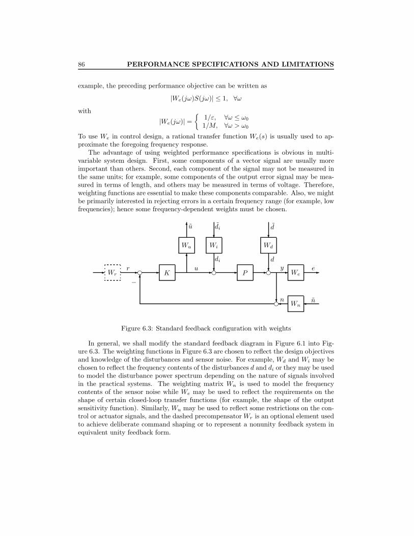
86 PERFORMANCE SPECIFICATIONS AND LIMITATIONS
example, the preceding performance objective can be written as
|We(jω)S(jω)| ≤ 1, ∀ω
with
|We(jω)| =
1/ε, ∀ω ≤ ω0
1/M, ∀ω > ω0
To use We in control design, a rational transfer function We(s) is usually used to ap-proximate the foregoing frequency response.
The advantage of using weighted performance specifications is obvious in multi-variable system design. First, some components of a vector signal are usually moreimportant than others. Second, each component of the signal may not be measured inthe same units; for example, some components of the output error signal may be mea-sured in terms of length, and others may be measured in terms of voltage. Therefore,weighting functions are essential to make these components comparable. Also, we mightbe primarily interested in rejecting errors in a certain frequency range (for example, lowfrequencies); hence some frequency-dependent weights must be chosen.
eeee
n
6
? n
eyu
d
ddiu
di
−
r
Wn
?
?Wd
-We--P
6
6
Wi
?
?
Wu
-K ---Wr-
Figure 6.3: Standard feedback configuration with weights
In general, we shall modify the standard feedback diagram in Figure 6.1 into Fig-ure 6.3. The weighting functions in Figure 6.3 are chosen to reflect the design objectivesand knowledge of the disturbances and sensor noise. For example, Wd and Wi may bechosen to reflect the frequency contents of the disturbances d and di or they may be usedto model the disturbance power spectrum depending on the nature of signals involvedin the practical systems. The weighting matrix Wn is used to model the frequencycontents of the sensor noise while We may be used to reflect the requirements on theshape of certain closed-loop transfer functions (for example, the shape of the outputsensitivity function). Similarly, Wu may be used to reflect some restrictions on the con-trol or actuator signals, and the dashed precompensator Wr is an optional element usedto achieve deliberate command shaping or to represent a nonunity feedback system inequivalent unity feedback form.

6.2. Weighted H2 and H∞ Performance 87
It is, in fact, essential that some appropriate weighting matrices be used in orderto utilize the optimal control theory discussed in this book (i.e., H2 and H∞ theory).So a very important step in the controller design process is to choose the appropriateweights, We,Wd,Wu, and possibly Wn,Wi, Wr . The appropriate choice of weights for aparticular practical problem is not trivial. In many occasions, as in the scalar case, theweights are chosen purely as a design parameter without any physical bases, so theseweights may be treated as tuning parameters that are chosen by the designer to achievethe best compromise between the conflicting objectives. The selection of the weightingmatrices should be guided by the expected system inputs and the relative importanceof the outputs.
Hence, control design may be regarded as a process of choosing a controller K suchthat certain weighted signals are made small in some sense. There are many differentways to define the smallness of a signal or transfer matrix, as we have discussed inthe last chapter. Different definitions lead to different control synthesis methods, andsome are much harder than others. A control engineer should make a judgment of themathematical complexity versus engineering requirements.
Next, we introduce two classes of performance formulations: H2 and H∞ criteria.For the simplicity of presentation, we shall assume that di = 0 and n = 0.
H2 Performance
Assume, for example, that the disturbance d can be approximately modeled as animpulse with random input direction; that is,
d(t) = ηδ(t)
andE(ηη∗) = I
where E denotes the expectation. We may choose to minimize the expected energy ofthe error e due to the disturbance d:
E‖e‖22
= E
∫ ∞0
‖e‖2 dt
= ‖WeSoWd‖22
In general, a controller minimizing only the above criterion can lead to a very largecontrol signal u that could cause saturation of the actuators as well as many otherundesirable problems. Hence, for a realistic controller design, it is necessary to includethe control signal u in the cost function. Thus, our design criterion would usually besomething like this:
E‖e‖22 + ρ2 ‖u‖22
=∥∥∥∥[ WeSoWd
ρWuKSoWd
]∥∥∥∥2
2
with some appropriate choice of weighting matrix Wu and scalar ρ. The parameter ρclearly defines the tradeoff we discussed earlier between good disturbance rejection at

88 PERFORMANCE SPECIFICATIONS AND LIMITATIONS
the output and control effort (or disturbance and sensor noise rejection at the actuators).Note that ρ can be set to ρ = 1 by an appropriate choice of Wu. This problem canbe viewed as minimizing the energy consumed by the system in order to reject thedisturbance d.
This type of problem was the dominant paradigm in the 1960s and 1970s and isusually referred to as linear quadratic Gaussian control, or simply as LQG. (Such prob-lems will also be referred to as H2 mixed-sensitivity problems for consistency with theH∞ problems discussed next.) The development of this paradigm stimulated extensiveresearch efforts and is responsible for important technological innovation, particularlyin the area of estimation. The theoretical contributions include a deeper understandingof linear systems and improved computational methods for complex systems throughstate-space techniques. The major limitation of this theory is the lack of formal treat-ment of uncertainty in the plant itself. By allowing only additive noise for uncertainty,the stochastic theory ignored this important practical issue. Plant uncertainty is par-ticularly critical in feedback systems. (See Paganini [1995,1996] for some recent resultson robust H2 control theory.)
H∞ Performance
Although the H2 norm (or L2 norm) may be a meaningful performance measure andalthough LQG theory can give efficient design compromises under certain disturbanceand plant assumptions, the H2 norm suffers a major deficiency. This deficiency is dueto the fact that the tradeoff between disturbance error reduction and sensor noise errorreduction is not the only constraint on feedback design. The problem is that theseperformance tradeoffs are often overshadowed by a second limitation on high loop gains— namely, the requirement for tolerance to uncertainties. Though a controller maybe designed using FDLTI models, the design must be implemented and operated witha real physical plant. The properties of physical systems (in particular, the ways inwhich they deviate from finite-dimensional linear models) put strict limitations on thefrequency range over which the loop gains may be large.
A solution to this problem would be to put explicit constraints on the loop gain inthe cost function. For instance, one may chose to minimize
sup‖d‖2≤1
‖e‖2 = ‖WeSoWd‖∞
subject to some restrictions on the control energy or control bandwidth:
sup‖d‖2
≤1
‖u‖2 = ‖WuKSoWd‖∞
Or, more frequently, one may introduce a parameter ρ and a mixed criterion
sup‖d‖
2≤1
‖e‖22 + ρ2 ‖u‖22
=∥∥∥∥[ WeSoWd
ρWuKSoWd
]∥∥∥∥2
∞

6.3. Selection of Weighting Functions 89
Alternatively, if the system robust stability margin is the major concern, the weightedcomplementary sensitivity has to be limited. Thus the whole cost function may be∥∥∥∥[ WeSoWd
ρW1ToW2
]∥∥∥∥∞
where W1 and W2 are the frequency-dependent uncertainty scaling matrices. Thesedesign problems are usually called H∞ mixed-sensitivity problems. For a scalar system,an H∞ norm minimization problem can also be viewed as minimizing the maximummagnitude of the system’s steady-state response with respect to the worst-case sinusoidalinputs.
6.3 Selection of Weighting Functions
The selection of weighting functions for a specific design problem often involves ad hocfixing, many iterations, and fine tuning. It is very hard to give a general formula forthe weighting functions that will work in every case. Nevertheless, we shall try to givesome guidelines in this section by looking at a typical SISO problem.
Consider an SISO feedback system shown in Figure 6.1. Then the tracking error ise = r − y = S(r − d) + Tn− SPdi. So, as we have discussed earlier, we must keep |S|small over a range of frequencies, typically low frequencies where r and d are significant.To motivate the choice of our performance weighting function We, let L = PK be astandard second-order system
L =ω2n
s(s+ 2ξωn)
It is well-known from the classical control theory that the quality of the (step) timeresponse can be quantified by rise time tr, settling time ts, and percent overshoot100Mp%. Furthermore, these performance indices can be approximately calculated as
tr ≈0.6 + 2.16ξ
ωn, 0.3 ≤ ξ ≤ 0.8; ts ≈
4ξωn
; Mp = e− πξ√
1−ξ2 , 0 < ξ < 1
The key points to note are that (1) the speed of the system response is proportional toωn and (2) the overshoot of the system response is determined only by the damping ratioξ. It is well known that the frequency ωn and the damping ratio ξ can be essentiallycaptured in the frequency domain by the open-loop crossover frequency and the phasemargin or the bandwidth and the resonant peak of the closed-loop complementarysensitivity function T .
Since our performance objectives are closely related to the sensitivity function, weshall consider in some detail how these time domain indices or, equivalently, ωn and ξare related to the frequency response of the sensitivity function
S =1
1 + L=
s(s+ 2ξωn)s2 + 2ξωns+ ω2
n
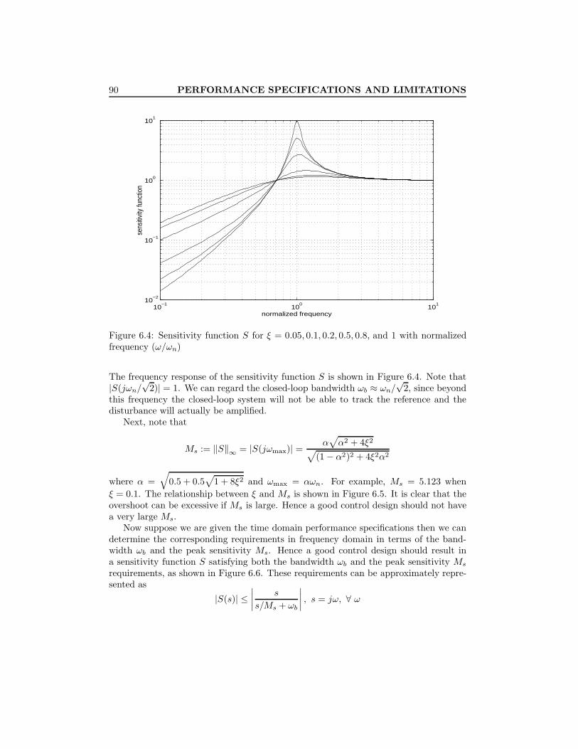
90 PERFORMANCE SPECIFICATIONS AND LIMITATIONS
10−1
100
101
10−2
10−1
100
101
normalized frequency
sens
itivi
ty fu
nctio
n
Figure 6.4: Sensitivity function S for ξ = 0.05, 0.1, 0.2, 0.5, 0.8, and 1 with normalizedfrequency (ω/ωn)
The frequency response of the sensitivity function S is shown in Figure 6.4. Note that|S(jωn/
√2)| = 1. We can regard the closed-loop bandwidth ωb ≈ ωn/
√2, since beyond
this frequency the closed-loop system will not be able to track the reference and thedisturbance will actually be amplified.
Next, note that
Ms := ‖S‖∞ = |S(jωmax)| = α√α2 + 4ξ2√
(1− α2)2 + 4ξ2α2
where α =√
0.5 + 0.5√
1 + 8ξ2 and ωmax = αωn. For example, Ms = 5.123 whenξ = 0.1. The relationship between ξ and Ms is shown in Figure 6.5. It is clear that theovershoot can be excessive if Ms is large. Hence a good control design should not havea very large Ms.
Now suppose we are given the time domain performance specifications then we candetermine the corresponding requirements in frequency domain in terms of the band-width ωb and the peak sensitivity Ms. Hence a good control design should result ina sensitivity function S satisfying both the bandwidth ωb and the peak sensitivity Ms
requirements, as shown in Figure 6.6. These requirements can be approximately repre-sented as
|S(s)| ≤∣∣∣∣ s
s/Ms + ωb
∣∣∣∣ , s = jω, ∀ ω

6.3. Selection of Weighting Functions 91
0 0.1 0.2 0.3 0.4 0.5 0.6 0.7 0.8 0.9 11
1.5
2
2.5
3
3.5
4
4.5
5
damping ratio
peak
sens
itivity
Figure 6.5: Peak sensitivity Ms versus damping ratio ξ
1
M
|S(jbω
s
ω)|
1/|We|
Figure 6.6: Performance weight We and desired S
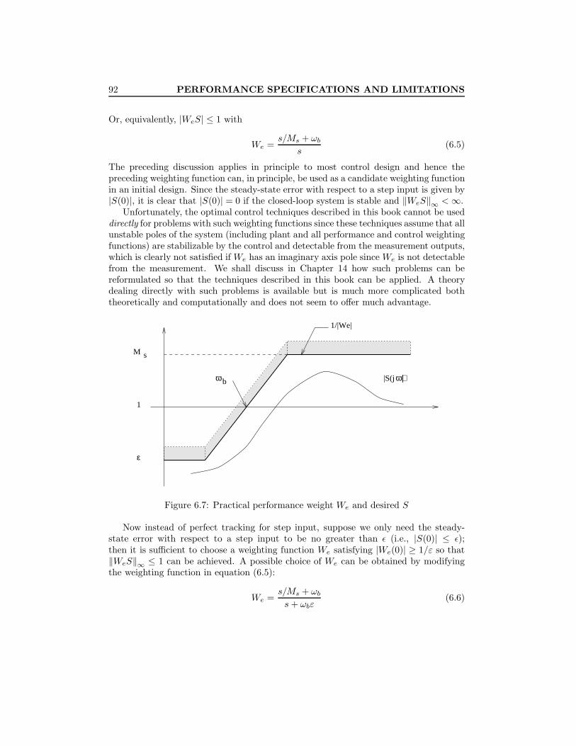
92 PERFORMANCE SPECIFICATIONS AND LIMITATIONS
Or, equivalently, |WeS| ≤ 1 with
We =s/Ms + ωb
s(6.5)
The preceding discussion applies in principle to most control design and hence thepreceding weighting function can, in principle, be used as a candidate weighting functionin an initial design. Since the steady-state error with respect to a step input is given by|S(0)|, it is clear that |S(0)| = 0 if the closed-loop system is stable and ‖WeS‖∞ <∞.
Unfortunately, the optimal control techniques described in this book cannot be useddirectly for problems with such weighting functions since these techniques assume that allunstable poles of the system (including plant and all performance and control weightingfunctions) are stabilizable by the control and detectable from the measurement outputs,which is clearly not satisfied if We has an imaginary axis pole since We is not detectablefrom the measurement. We shall discuss in Chapter 14 how such problems can bereformulated so that the techniques described in this book can be applied. A theorydealing directly with such problems is available but is much more complicated boththeoretically and computationally and does not seem to offer much advantage.
sM
1
|S(jb
ε
ω
1/|We|
ω)|
Figure 6.7: Practical performance weight We and desired S
Now instead of perfect tracking for step input, suppose we only need the steady-state error with respect to a step input to be no greater than ε (i.e., |S(0)| ≤ ε);then it is sufficient to choose a weighting function We satisfying |We(0)| ≥ 1/ε so that‖WeS‖∞ ≤ 1 can be achieved. A possible choice of We can be obtained by modifyingthe weighting function in equation (6.5):
We =s/Ms + ωbs+ ωbε
(6.6)

6.3. Selection of Weighting Functions 93
Hence, for practical purpose, one can usually choose a suitable ε, as shown in Figure 6.7,to satisfy the performance specifications. If a steeper transition between low-frequencyand high-frequency is desired, the weight We can be modified as follows:
We =(s/ k√Ms + ωb
s+ ωb k√ε
)k(6.7)
for some integer k ≥ 1.The selection of control weighting function Wu follows similarly from the preceding
discussion by considering the control signal equation
u = KS(r− n− d)− Tdi
The magnitude of |KS| in the low-frequency range is essentially limited by the allowablecost of control effort and saturation limit of the actuators; hence, in general, the max-imum gain Mu of KS can be fairly large, while the high-frequency gain is essentiallylimited by the controller bandwidth (ωbc) and the (sensor) noise frequencies. Ideally,one would like to roll off as fast as possible beyond the desired control bandwidth sothat the high-frequency noises are attenuated as much as possible. Hence a candidateweight Wu would be
Wu =s+ ωbc/Mu
ωbc(6.8)
ε
bc
M
1
1
u
u
ω
1/|W |
|KS(j ω)|
Figure 6.8: Control weight Wu and desired KS
However, again the optimal control design techniques developed in this book cannotbe applied directly to a problem with an improper control weighting function. Hence

94 PERFORMANCE SPECIFICATIONS AND LIMITATIONS
we shall introduce a far away pole to make Wu proper:
Wu =s+ ωbc/Mu
ε1s+ ωbc(6.9)
for a small ε1 > 0, as shown in Figure 6.8. Similarly, if a faster rolloff is desired, onemay choose
Wu =(s+ ωbc/
k√Mu
k√ε1s+ ωbc
)k(6.10)
for some integer k ≥ 1.The weights for MIMO problems can be initially chosen as diagonal matrices with
each diagonal term chosen in the foregoing form.
6.4 Bode’s Gain and Phase Relation
One important problem that arises frequently is concerned with the level of perfor-mance that can be achieved in feedback design. It has been shown in Section 6.1 thatthe feedback design goals are inherently conflicting, and a tradeoff must be performedamong different design objectives. It is also known that the fundamental requirements,such as stability and robustness, impose inherent limitations on the feedback propertiesirrespective of design methods, and the design limitations become more severe in thepresence of right-half plane zeros and poles in the open-loop transfer function.
In the classical feedback theory, Bode’s gain-phase integral relation (see Bode [1945])has been used as an important tool to express design constraints in scalar systems. Thisintegral relation says that the phase of a stable and minimum phase transfer functionis determined uniquely by the magnitude of the transfer function. More precisely, letL(s) be a stable and minimum phase transfer function: then
∠L(jω0) =1π
∫ ∞−∞
d ln |L|dν
ln coth|ν|2dν (6.11)
where ν := ln(ω/ω0). The function ln coth|ν|2
= lne|ν|/2 + e−|ν|/2
e|ν|/2 − e−|ν|/2 is plotted in Fig-
ure 6.9.
Note that ln coth|ν|2
decreases rapidly as ω deviates from ω0 and hence the integral
depends mostly on the behavior ofd ln |L(jω)|
dνnear the frequency ω0. This is clear
from the following integration:
1π
∫ α
−αln coth
|ν|2dν =
1.1406 (rad), α = ln 31.3146 (rad), α = ln 51.443 (rad), α = ln 10
=
65.3o, α = ln 375.3o, α = ln 582.7o, α = ln 10.
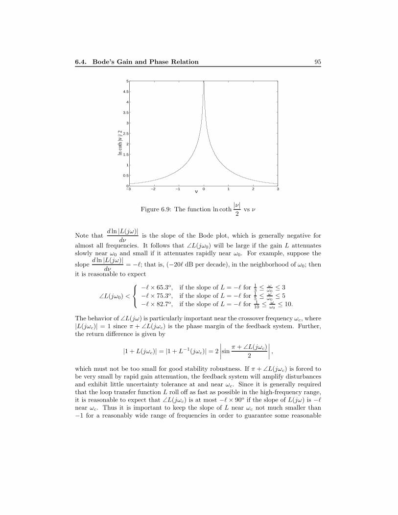
6.4. Bode’s Gain and Phase Relation 95
−3 −2 −1 0 1 2 30
0.5
1
1.5
2
2.5
3
3.5
4
4.5
5
ν
ln c
oth
|ν |/
2
Figure 6.9: The function ln coth|ν|2
vs ν
Note thatd ln |L(jω)|
dνis the slope of the Bode plot, which is generally negative for
almost all frequencies. It follows that ∠L(jω0) will be large if the gain L attenuatesslowly near ω0 and small if it attenuates rapidly near ω0. For example, suppose the
sloped ln |L(jω)|
dν= −`; that is, (−20` dB per decade), in the neighborhood of ω0; then
it is reasonable to expect
∠L(jω0) <
−`× 65.3o, if the slope of L = −` for 1
3 ≤ωω0≤ 3
−`× 75.3o, if the slope of L = −` for 15 ≤
ωω0≤ 5
−`× 82.7o, if the slope of L = −` for 110 ≤
ωω0≤ 10.
The behavior of ∠L(jω) is particularly important near the crossover frequency ωc, where|L(jωc)| = 1 since π + ∠L(jωc) is the phase margin of the feedback system. Further,the return difference is given by
|1 + L(jωc)| = |1 + L−1(jωc)| = 2∣∣∣∣sin π + ∠L(jωc)
2
∣∣∣∣ ,which must not be too small for good stability robustness. If π + ∠L(jωc) is forced tobe very small by rapid gain attenuation, the feedback system will amplify disturbancesand exhibit little uncertainty tolerance at and near ωc. Since it is generally requiredthat the loop transfer function L roll off as fast as possible in the high-frequency range,it is reasonable to expect that ∠L(jωc) is at most −`× 90o if the slope of L(jω) is −`near ωc. Thus it is important to keep the slope of L near ωc not much smaller than−1 for a reasonably wide range of frequencies in order to guarantee some reasonable

96 PERFORMANCE SPECIFICATIONS AND LIMITATIONS
performance. The conflict between attenuation rate and loop quality near crossover isthus clearly evident.
Bode’s gain and phase relation can be extended to stable and nonminimum phasetransfer functions easily. Let z1, z2, . . . , zk be the right-half plane zeros of L(s), then Lcan be factorized as
L(s) =−s+ z1
s+ z1
−s+ z2
s+ z2· · · −s+ zk
s+ zkLmp(s)
where Lmp is stable and minimum phase and |L(jω)| = |Lmp(jω)|. Hence
∠L(jω0) = ∠Lmp(jω0) + ∠k∏i=1
−jω0 + zijω0 + zi
=1π
∫ ∞−∞
d ln |Lmp|dν
ln coth|ν|2dν +
k∑i=1
∠−jω0 + zijω0 + zi
,
which gives
∠L(jω0) =1π
∫ ∞−∞
d ln |L|dν
ln coth|ν|2dν +
k∑i=1
∠−jω0 + zijω0 + zi
. (6.12)
Since ∠−jω0 + zijω0 + zi
≤ 0 for each i, a nonminimum phase zero contributes an additional
phase lag and imposes limitations on the rolloff rate of the open-loop gain. For example,suppose L has a zero at z > 0; then
φ1(ω0/z) := ∠−jω0 + z
jω0 + z
∣∣∣∣ω0=z,z/2,z/4
= −90o,−53.13o,−28o,
as shown in Figure 6.10. Since the slope of |L| near the crossover frequency is, ingeneral, no greater than −1, which means that the phase due to the minimum phasepart, Lmp, of L will, in general, be no greater than −90o, the crossover frequency (orthe closed-loop bandwidth) must satisfy
ωc < z/2 (6.13)
in order to guarantee the closed-loop stability and some reasonable closed-loop perfor-mance.
Next suppose L has a pair of complex right-half zeros at z = x± jy with x > 0; then
φ2(ω0/|z|) := ∠−jω0 + z
jω0 + z
−jω0 + z
jω0 + z
∣∣∣∣ω0=|z|,|z|/2,|z|/3,|z|/4
≈
−180o, −106.26o, −73.7o, −56o, Re(z) =(z)−180o, −86.7o, −55.9o, −41.3o, Re(z) ≈ =(z)−360o, 0o, 0o, 0o, Re(z) =(z)

6.4. Bode’s Gain and Phase Relation 97
0 0.1 0.2 0.3 0.4 0.5 0.6 0.7 0.8 0.9 1−90
−80
−70
−60
−50
−40
−30
−20
−10
0
ω0 / |z|
ph
ase
φ 1(ω
0 /z)
(in
deg
ree
)
Figure 6.10: Phase φ1(ω0/z) due to a real zero z > 0
0 0.1 0.2 0.3 0.4 0.5 0.6 0.7 0.8 0.9 1−200
−180
−160
−140
−120
−100
−80
−60
−40
−20
0
ω0 / |z|
phase φ 2
( ω
0 /
|z| )
(in
deg
ree
)
y/x=0.01 y/x=0.01
y/x=1
y/x=0.01
y/x=1 y/x=3
y/x=0.01
y/x=1 y/x=3
y/x=10
y/x=0.01
y/x=1 y/x=3
y/x=10 y/x=100
Figure 6.11: Phase φ2(ω0/|z|) due to a pair of complex zeros: z = x± jy and x > 0

98 PERFORMANCE SPECIFICATIONS AND LIMITATIONS
as shown in Figure 6.11. In this case we conclude that the crossover frequency mustsatisfy
ωc <
|z|/4, Re(z) =(z)|z|/3, Re(z) ≈ =(z)|z|, Re(z) =(z)
(6.14)
in order to guarantee the closed-loop stability and some reasonable closed-loop perfor-mance.
6.5 Bode’s Sensitivity Integral
In this section, we consider the design limitations imposed by the bandwidth constraintsand the right-half plane poles and zeros using Bode’s sensitivity integral and Poissonintegral. Let L be the open-loop transfer function with at least two more poles thanzeros and let p1, p2, . . . , pm be the open right-half plane poles of L. Then the followingBode’s sensitivity integral holds:∫ ∞
0
ln |S(jω)|dω = πm∑i=1
Re(pi) (6.15)
In the case where L is stable, the integral simplifies to∫ ∞0
ln |S(jω)|dω = 0 (6.16)
These integrals show that there will exist a frequency range over which the magnitudeof the sensitivity function exceeds one if it is to be kept below one at other frequencies,as illustrated in Figure 6.12. This is the so-called water bed effect.
1
|S(j
ω
ω)|
−
+
Figure 6.12: Water bed effect of sensitivity function

6.5. Bode’s Sensitivity Integral 99
Suppose that the feedback system is designed such that the level of sensitivity re-duction is given by
|S(jω)| ≤ ε < 1, ∀ω ∈ [0, ωl]
where ε > 0 is a given constant.Bandwidth constraints in feedback design typically require that the open-loop trans-
fer function be small above a specified frequency, and that it roll off at a rate of morethan one pole-zero excess above that frequency. These constraints are commonly neededto ensure stability robustness despite the presence of modeling uncertainty in the plantmodel, particularly at high frequencies. One way of quantifying such bandwidth con-straints is by requiring the open-loop transfer function to satisfy
|L(jω)| ≤ Mh
ω1+β≤ ε < 1, ∀ω ∈ [ωh, ∞)
where ωh > ωl, and Mh > 0, β > 0 are some given constants.Note that for ω ≥ ωh,
|S(jω)| ≤ 11− |L(jω)| ≤
11− Mh
ω1+β
and
−∫ ∞ωh
ln(
1− Mh
ω1+β
)dω =
∞∑i=1
∫ ∞ωh
1i
(Mh
ω1+β
)idω
=∞∑i=1
1i
ωhi(1 + β)− 1
(Mh
ω1+βh
)i
≤ ωhβ
∞∑i=1
1i
(Mh
ω1+βh
)i= −ωh
βln
(1− Mh
ω1+βh
)≤ −ωh
βln(1− ε).
Then
πm∑i=1
Re(pi) =∫ ∞
0
ln |S(jω)|dω
=∫ ωl
0
ln |S(jω)|dω +∫ ωh
ωl
ln |S(jω)|dω +∫ ∞ωh
ln |S(jω)|dω
≤ ωl ln ε+ (ωh − ωl) maxω∈[ωl,ωh]
ln |S(jω)| −∫ ∞ωh
ln(
1− Mh
ω1+β
)dω
≤ ωl ln ε+ (ωh − ωl) maxω∈[ωl,ωh]
ln |S(jω)| − ωhβ
ln(1− ε),

100 PERFORMANCE SPECIFICATIONS AND LIMITATIONS
which gives
maxω∈[ωl,ωh]
|S(jω)| ≥ eα(
1ε
) ωlωh−ωl
(1− ε)ωh
β(ωh−ωl)
where
α =π∑mi=1 Re(pi)ωh − ωl
.
The above lower bound shows that the sensitivity can be very significant in the transitionband.
Next, using the Poisson integral relation, we investigate the design constraints onsensitivity properties imposed by open-loop nonminimum phase zeros. Suppose L hasat least one more poles than zeros and suppose z = x0 + jy0 with x0 > 0 is a right-halfplane zero of L. Then∫ ∞
−∞ln |S(jω)| x0
x20 + (ω − y0)2
dω = π lnm∏i=1
∣∣∣∣z + piz − pi
∣∣∣∣ (6.17)
This integral implies that the sensitivity reduction ability of the system may be severelylimited by the open-loop unstable poles and nonminimum phase zeros, especially whenthese poles and zeros are close to each other.
Define
θ(z) :=∫ ωl
−ωl
x0
x20 + (ω − y0)2
dω
Then
π lnm∏i=1
∣∣∣∣z + piz − pi
∣∣∣∣ =∫ ∞−∞
ln |S(jω)| x0
x20 + (ω − y0)2
dω
≤ (π − θ(z)) ln ‖S(jω)‖∞ + θ(z) ln(ε),
which gives
‖S(s)‖∞ ≥(
1ε
) θ(z)π−θ(z)
(m∏i=1
∣∣∣∣z + piz − pi
∣∣∣∣) ππ−θ(z)
This lower bound on the maximum sensitivity shows that for a nonminimum phasesystem, its sensitivity must increase significantly beyond one at certain frequencies ifthe sensitivity reduction is to be achieved at other frequencies.
6.6 Analyticity Constraints
Let p1, p2, . . . , pm and z1, z2, . . . , zk be the open right-half plane poles and zeros of L,respectively. Suppose that the closed-loop system is stable. Then
S(pi) = 0, T (pi) = 1, i = 1, 2, . . . ,m

6.6. Analyticity Constraints 101
andS(zj) = 1, T (zj) = 0, j = 1, 2, . . . , k
The internal stability of the feedback system is guaranteed by satisfying these analyticity(or interpolation) conditions. On the other hand, these conditions also impose severelimitations on the achievable performance of the feedback system.
Suppose S = (I +L)−1 and T = L(I +L)−1 are stable. Then p1, p2, . . . , pm are theright-half plane zeros of S and z1, z2, . . . , zk are the right-half plane zeros of T . Let
Bp(s) =m∏i=1
s− pis+ pi
, Bz(s) =k∏j=1
s− zjs+ zj
Then |Bp(jω)| = 1 and |Bz(jω)| = 1 for all frequencies and, moreover,
B−1p (s)S(s) ∈ H∞, B−1
z (s)T (s) ∈ H∞.Hence, by the maximum modulus theorem, we have
‖S(s)‖∞ =∥∥B−1
p (s)S(s)∥∥∞ ≥ |B
−1p (z)S(z)|
for any z with Re(z) > 0. Let z be a right-half plane zero of L; then
‖S(s)‖∞ ≥ |B−1p (z)| =
m∏i=1
∣∣∣∣z + piz − pi
∣∣∣∣Similarly, one can obtain
‖T (s)‖∞ ≥ |B−1z (p)| =
k∏j=1
∣∣∣∣p+ zjp− zj
∣∣∣∣where p is a right-half plane pole of L.
The weighted problem can be considered in the same fashion. Let We be a weightsuch that WeS is stable. Then
‖We(s)S(s)‖∞ ≥ |We(z)|m∏i=1
∣∣∣∣z + piz − pi
∣∣∣∣Now suppose We(s) =
s/Ms + ωbs+ ωbε
, ‖WeS‖∞ ≤ 1, and z is a real right-half plane zero.
Thenz/Ms + ωbz + ωbε
≤m∏i=1
∣∣∣∣z − piz + pi
∣∣∣∣ =: α,
which gives
ωb ≤z
1− αε (α− 1Ms
) ≈ z(α− 1Ms
)
where α = 1 if L has no right-half plane poles. This shows that the bandwidth of theclosed-loop must be much smaller than the right-half plane zero. Similar conclusionscan be arrived at for complex right-half plane zeros.

102 PERFORMANCE SPECIFICATIONS AND LIMITATIONS
6.7 Notes and References
The loop-shaping design is well-known for SISO systems in the classical control theory.The idea was extended to MIMO systems by Doyle and Stein [1981] using the LQGdesign technique. The limitations of the loop-shaping design are discussed in detail inStein and Doyle [1991]. Chapter 16 presents another loop-shaping method using H∞control theory, which has the potential to overcome the limitations of the LQG/LTRmethod. Some additional discussions on the choice of weighting functions can be foundin Skogestad and Postlethwaite [1996]. The design tradeoffs and limitations for SISOsystems are discussed in detail in Bode [1945], Horowitz [1963], and Doyle, Francis,and Tannenbaum [1992]. The monograph by Freudenberg and Looze [1988] containsmany multivariable generalizations. The multivariable generalization of Bode’s integralrelation can be found in Chen [1995], on which Section 6.5 is based. Some related resultscan be found in Boyd and Desoer [1985]. Additional related results can be found in arecent book by Seron, Braslavsky, and Goodwin [1997].
6.8 Problems
Problem 6.1 Let P be an open-loop plant. It is desired to design a controller so thatthe overshoot ≤ 10% and settling time ≤ 10 sec. Estimate the allowable peak sensitivityMs and the closed-loop bandwidth.
Problem 6.2 Let L1 =1
s(s+ 1)2be an open-loop transfer function of a unity feedback
system. Find the phase margin, overshoot, settling time, and the corresponding Ms.
Problem 6.3 Repeat Problem 6.2 with
L2 =100(s+ 10)
(s+ 1)(s+ 2)(s+ 20).
Problem 6.4 Let P =10(1− s)s(s+ 10)
. Use classical loop-shaping method to design a first-
order lead or lag controller so that the system has at least 30o phase margin and aslarge a crossover frequency as possible.
Problem 6.5 Use the root locus method to show that a nonminimum phase systemcannot be stabilized by a very high-gain controller.
Problem 6.6 Let P =5
(1− s)(s+ 2). Design a lead or lag controller so that the system
has at least 30o phase margin with loop gain ≥ 2 for any frequency ω ≤ 0.1 and thesmallest possible bandwidth (or crossover frequency).
Problem 6.7 Use the root locus method to show that an unstable system cannot bestabilized by a very low gain controller.

6.8. Problems 103
Problem 6.8 Consider the unity-feedback loop with proper controllerK(s) and strictlyproper plant P (s), both assumed square. Assume internal stability.
1. Let w(s) be a scalar weighting function, assumed in RH∞. Define
ε = ‖w(I + PK)−1‖∞, δ = ‖K(I + PK)−1‖∞
so ε measures, say, disturbance attenuation and δ measures, say, control effort.Derive the following inequality, which shows that ε and δ cannot both be smallsimultaneously in general. For every Re s0 ≥ 0
|w(s0)| ≤ ε+ |w(s0)|σmin[P (s0)]δ.
2. If we want very good disturbance attenuation at a particular frequency, you mightguess that we need high controller gain at that frequency. Fix ω with jω not apole of P (s), and suppose
ε := σmax[(I + PK)−1(jω)] < 1.
Derive a lower bound for σmin[K(jω)]. This lower bound should blow up as ε→ 0.
Problem 6.9 Suppose that P is proper and has one right half plane zero at s = z > 0.Suppose that y = w
1+PK , where w is a unit step at time t = 0, and that our performancespecification is
|y(t)| ≤
α, if 0 ≤ t ≤ T ;β, if T < t
for some α > 1 > β > 0. Show that for a proper, internally stabilizing, LTI controllerK to exist that meets the specification, we must have that
ln(α− βα− 1
)≤ zT.
What tradeoffs does this imply?
Problem 6.10 Let K be a stabilizing controller for the plant
P =s− α
(s− β)(s+ γ)
α > 0, β > 0, γ ≥ 0. Suppose |S(jω)| ≤ δ < 1, ∀ω ∈ [−ω0, ω0] where
S(s) =1
1 + PK.
Find a lower bound for ‖S‖∞ and calculate the lower bound for α = 1, β = 2, γ = 10,δ = 0.2, and ω0 = 1.

104 PERFORMANCE SPECIFICATIONS AND LIMITATIONS

Chapter 7
Balanced Model Reduction
Simple linear models/controllers are normally preferred over complex ones in controlsystem design for some obvious reasons: They are much easier to do analysis andsynthesis with. Furthermore, simple controllers are easier to implement and are morereliable because there are fewer things to go wrong in the hardware or bugs to fix inthe software. In the case when the system is infinite dimensional, the model/controllerapproximation becomes essential. In this chapter we consider the problem of reducingthe order of a linear multivariable dynamical system. There are many ways to reduce theorder of a dynamical system. However, we shall study only one of them: the balancedtruncation method. The main advantage of this method is that it is simple and performsfairly well.
A model order-reduction problem can, in general, be stated as follows: Given a full-order model G(s), find a lower-order model (say, an rth order model Gr), such that Gand Gr are close in some sense. Of course, there are many ways to define the closenessof an approximation. For example, one may desire that the reduced model be such that
G = Gr + ∆a
and ∆a is small in some norm. This model reduction is usually called an additive modelreduction problem. We shall be only interested in L∞ norm approximation in this book.Once the norm is chosen, the additive model reduction problem can be formulated as
infdeg(Gr)≤r
‖G−Gr‖∞ .
In general, a practical model reduction problem is inherently frequency-weighted (i.e.,the requirement on the approximation accuracy at one frequency range can be drasticallydifferent from the requirement at another frequency range). These problems can, ingeneral, be formulated as frequency-weighted model reduction problems:
infdeg(Gr)≤r
‖Wo(G−Gr)Wi‖∞
105

106 BALANCED MODEL REDUCTION
with an appropriate choice of Wi and Wo. We shall see in this chapter how the bal-anced realization can give an effective approach to the aforementioned model reductionproblems.
7.1 Lyapunov Equations
Testing stability, controllability, and observability of a system is very important in linearsystem analysis and synthesis. However, these tests often have to be done indirectly. Inthat respect, the Lyapunov theory is sometimes useful. Consider the following Lyapunovequation:
A∗Q+QA+H = 0 (7.1)
with given real matrices A and H. It is well known that this equation has a uniquesolution iff λi(A) + λj(A) 6= 0,∀i, j. In this section, we shall study the relationshipsbetween the solution Q and the stability of A. The following results are standard.
Lemma 7.1 Assume that A is stable, then the following statements hold:
(i) Q =∫∞
0eA∗tHeAtdt.
(ii) Q > 0 if H > 0 and Q ≥ 0 if H ≥ 0.
(iii) If H ≥ 0, then (H,A) is observable iff Q > 0.
An immediate consequence of part (iii) is that, given a stable matrix A, a pair (C,A)is observable if and only if the solution to the following Lyapunov equation
A∗Q+QA+ C∗C = 0
is positive definite, where Q is the observability Gramian. Similarly, a pair (A,B) iscontrollable if and only if the solution to
AP + PA∗ +BB∗ = 0
is positive definite, where P is the controllability Gramian.In many applications, we are given the solution of the Lyapunov equation and need
to conclude the stability of the matrix A.
Lemma 7.2 Suppose Q is the solution of the Lyapunov equation (7.1), then
(i) Reλi(A) ≤ 0 if Q > 0 and H ≥ 0.
(ii) A is stable if Q > 0 and H > 0.
(iii) A is stable if Q ≥ 0, H ≥ 0, and (H,A) is detectable.

7.2. Balanced Realizations 107
Proof. Let λ be an eigenvalue of A and v 6= 0 be a corresponding eigenvector, thenAv = λv. Premultiply equation (7.1) by v∗ and postmultiply equation (7.1) by v to get
2Re λ(v∗Qv) + v∗Hv = 0.
Now if Q > 0, then v∗Qv > 0, and it is clear that Reλ ≤ 0 if H ≥ 0 and Reλ < 0 ifH > 0. Hence (i) and (ii) hold. To see (iii), we assume Reλ ≥ 0. Then we must havev∗Hv = 0 (i.e., Hv = 0). This implies that λ is an unstable and unobservable mode,which contradicts the assumption that (H,A) is detectable. 2
7.2 Balanced Realizations
Although there are infinitely many different state-space realizations for a given transfermatrix, some particular realizations have proven to be very useful in control engineeringand signal processing. Here we will only introduce one class of realizations for stabletransfer matrices that are most useful in control applications. To motivate the class ofrealizations, we first consider some simple facts.
Lemma 7.3 Let[A BC D
]be a state-space realization of a (not necessarily stable)
transfer matrix G(s). Suppose that there exists a symmetric matrix
P = P ∗ =[P1 00 0
]with P1 nonsingular such that
AP + PA∗ +BB∗ = 0.
Now partition the realization (A,B,C,D) compatibly with P as A11 A12 B1
A21 A22 B2
C1 C2 D
.Then
[A11 B1
C1 D
]is also a realization of G. Moreover, (A11, B1) is controllable if A11
is stable.
Proof. Use the partitioned P and (A,B,C) to get
0 = AP + PA∗ +BB∗ =[A11P1 + P1A
∗11 +B1B
∗1 P1A
∗21 +B1B
∗2
A21P1 +B2B∗1 B2B
∗2
],

108 BALANCED MODEL REDUCTION
which gives B2 = 0 and A21 = 0 since P1 is nonsingular. Hence, part of the realizationis not controllable: A11 A12 B1
A21 A22 B2
C1 C2 D
=
A11 A12 B1
0 A22 0C1 C2 D
=[A11 B1
C1 D
].
Finally, it follows from Lemma 7.1 that (A11, B1) is controllable if A11 is stable. 2
We also have the following:
Lemma 7.4 Let[A BC D
]be a state-space realization of a (not necessarily stable)
transfer matrix G(s). Suppose that there exists a symmetric matrix
Q = Q∗ =[Q1 00 0
]with Q1 nonsingular such that
QA+A∗Q+ C∗C = 0.
Now partition the realization (A,B,C,D) compatibly with Q as A11 A12 B1
A21 A22 B2
C1 C2 D
.Then
[A11 B1
C1 D
]is also a realization of G. Moreover, (C1, A11) is observable if A11
is stable.
The preceding two lemmas suggest that to obtain a minimal realization from a stablenonminimal realization, one only needs to eliminate all states corresponding to the zeroblock diagonal term of the controllability Gramian P and the observability GramianQ. In the case where P is not block diagonal, the following procedure can be used toeliminate noncontrollable subsystems:
1. Let G(s) =[A BC D
]be a stable realization.
2. Compute the controllability Gramian P ≥ 0 from
AP + PA∗ +BB∗ = 0.
3. Diagonalize P to get P =[U1 U2
] [ Λ1 00 0
] [U1 U2
]∗ with Λ1 > 0 and[U1 U2
]unitary.

7.2. Balanced Realizations 109
4. Then G(s) =[U∗1AU1 U∗1BCU1 D
]is a controllable realization.
A dual procedure can also be applied to eliminate nonobservable subsystems.
Now assume that Λ1 > 0 is diagonal and is partitioned as Λ1 = diag(Λ11,Λ12) suchthat λmax(Λ12) λmin(Λ11); then it is tempting to conclude that one can also discardthose states corresponding to Λ12 without causing much error. However, this is notnecessarily true, as shown in the following example.
Example 7.1 Consider a stable transfer function
G(s) =3s+ 18
s2 + 3s+ 18.
Then G(s) has a state-space realization given by
G(s) =
−1 −4/α 14α −2 2α−1 2/α 0
where α is any nonzero number. It is easy to check that the controllability Gramian ofthe realization is given by
P =[
0.5α2
].
Since the last diagonal term of P can be made arbitrarily small by making α small,the controllability of the corresponding state can be made arbitrarily weak. If the statecorresponding to the last diagonal term of P is removed, we get a transfer function
G =[−1 1−1 0
]=−1s+ 1
,
which is not close to the original transfer function in any sense. The problem may beeasily detected if one checks the observability Gramian Q, which is
Q =[
0.51/α2
].
Since 1/α2 is very large if α is small, this shows that the state corresponding to the lastdiagonal term is strongly observable.
This example shows that the controllability (or observability) Gramian alone cannotgive an accurate indication of the dominance of the system states in the input/output

110 BALANCED MODEL REDUCTION
behavior. This motivates the introduction of a balanced realization that gives balancedGramians for controllability and observability.
Suppose G =[A BC D
]is stable (i.e., A is stable). Let P and Q denote the
controllability Gramian and observability Gramian, respectively. Then by Lemma 7.1,P and Q satisfy the following Lyapunov equations:
AP + PA∗ +BB∗ = 0 (7.2)
A∗Q+QA+ C∗C = 0, (7.3)
and P ≥ 0, Q ≥ 0. Furthermore, the pair (A,B) is controllable iff P > 0, and (C,A) isobservable iff Q > 0.
Suppose the state is transformed by a nonsingular T to x = Tx to yield the realiza-tion
G =
[A B
C D
]=[TAT−1 TBCT−1 D
].
Then the Gramians are transformed to P = TPT ∗ and Q = (T−1)∗QT−1. Note thatP Q = TPQT−1, and therefore the eigenvalues of the product of the Gramians areinvariant under state transformation.
Consider the similarity transformation T , which gives the eigenvector decomposition
PQ = T−1ΛT, Λ = diag(λ1Is1 , . . . , λNIsN ).
Then the columns of T−1 are eigenvectors of PQ corresponding to the eigenvalues λi.Later, it will be shown that PQ has a real diagonal Jordan form and that Λ ≥ 0, whichare consequences of P ≥ 0 and Q ≥ 0.
Although the eigenvectors are not unique, in the case of a minimal realization theycan always be chosen such that
P = TPT ∗ = Σ,
Q = (T−1)∗QT−1 = Σ,
where Σ = diag(σ1Is1 , σ2Is2 , . . . , σNIsN ) and Σ2 = Λ. This new realization with con-trollability and observability Gramians P = Q = Σ will be referred to as a balancedrealization (also called internally balanced realization). The decreasingly ordered num-bers, σ1 > σ2 > . . . > σN ≥ 0, are called the Hankel singular values of the system.
More generally, if a realization of a stable system is not minimal, then there is a trans-formation such that the controllability and observability Gramians for the transformedrealization are diagonal and the controllable and observable subsystem is balanced. Thisis a consequence of the following matrix fact.

7.2. Balanced Realizations 111
Theorem 7.5 Let P and Q be two positive semidefinite matrices. Then there exists anonsingular matrix T such that
TPT ∗ =
Σ1
Σ2
00
, (T−1)∗QT−1 =
Σ1
0Σ3
0
respectively, with Σ1, Σ2, Σ3 diagonal and positive definite.
Proof. Since P is a positive semidefinite matrix, there exists a transformation T1 suchthat
T1PT∗1 =
[I 00 0
]Now let
(T ∗1 )−1QT−11 =
[Q11 Q12
Q∗12 Q22
]and there exists a unitary matrix U1 such that
U1Q11U∗1 =
[Σ2
1 00 0
], Σ1 > 0
Let
(T ∗2 )−1 =[U1 00 I
]and then
(T ∗2 )−1(T ∗1 )−1QT−11 (T2)−1 =
Σ21 0 Q121
0 0 Q122
Q∗121 Q∗122 Q22
But Q ≥ 0 implies Q122 = 0. So now let
(T ∗3 )−1 =
I 0 00 I 0
−Q∗121Σ−21 0 I
giving
(T ∗3 )−1(T ∗2 )−1(T ∗1 )−1QT−11 (T2)−1(T3)−1 =
Σ21 0 0
0 0 00 0 Q22 − Q∗121Σ−2
1 Q121
Next find a unitary matrix U2 such that
U2(Q22 − Q∗121Σ−21 Q121)U∗2 =
[Σ3 00 0
], Σ3 > 0

112 BALANCED MODEL REDUCTION
Define
(T ∗4 )−1 =
Σ−1/21 0 00 I 00 0 U2
and let
T = T4T3T2T1
Then
TPT ∗ =
Σ1
Σ2
00
, (T ∗)−1QT−1 =
Σ1
0Σ3
0
with Σ2 = I. 2
Corollary 7.6 The product of two positive semidefinite matrices is similar to a positivesemidefinite matrix.
Proof. Let P and Q be any positive semidefinite matrices. Then it is easy to see thatwith the transformation given previously
TPQT−1 =[
Σ21 0
0 0
]2
Corollary 7.7 For any stable system G =[A BC D
], there exists a nonsingular trans-
formation T such that G =
[TAT−1 TB
CT−1 D
]has controllability Gramian P and ob-
servability Gramian Q given by
P =
Σ1
Σ2
00
, Q =
Σ1
0Σ3
0
respectively, with Σ1, Σ2, Σ3 diagonal and positive definite.

7.2. Balanced Realizations 113
In the special case where[A BC D
]is a minimal realization, a balanced realization
can be obtained through the following simplified procedure:
1. Compute the controllability and observability Gramians P > 0, Q > 0.
2. Find a matrix R such that P = R∗R.
3. Diagonalize RQR∗ to get RQR∗ = UΣ2U∗.
4. Let T−1 = R∗UΣ−1/2. Then TPT ∗ = (T ∗)−1QT−1 = Σ and
[TAT−1 TB
CT−1 D
]is balanced.
Assume that the Hankel singular values of the system are decreasingly ordered sothat Σ = diag(σ1Is1 , σ2Is2 , . . . , σNIsN ) with σ1 > σ2 > . . . > σN and suppose σr σr+1 for some r. Then the balanced realization implies that those states correspondingto the singular values of σr+1, . . . , σN are less controllable and less observable than thosestates corresponding to σ1, . . . , σr. Therefore, truncating those less controllable and lessobservable states will not lose much information about the system.
Two other closely related realizations are called input normal realization with P = Iand Q = Σ2, and output normal realization with P = Σ2 and Q = I. Both realizationscan be obtained easily from the balanced realization by a suitable scaling on the states.
Next we shall derive some simple and useful bounds for the H∞ norm and the L1
norm of a stable system.
Theorem 7.8 Suppose
G(s) =[A BC 0
]∈ RH∞
is a balanced realization; that is, there exists
Σ = diag(σ1Is1 , σ2Is2 , . . . , σN IsN ) ≥ 0
with σ1 > σ2 > . . . > σN ≥ 0, such that
AΣ + ΣA∗ +BB∗ = 0 A∗Σ + ΣA+ C∗C = 0
Then
σ1 ≤ ‖G‖∞ ≤∫ ∞
0
‖g(t)‖ dt ≤ 2N∑i=1
σi
where g(t) = CeAtB.
Remark 7.1 It should be clear that the inequalities stated in the theorem do notdepend on a particular state-space realization of G(s). However, use of the balancedrealization does make the proof simple. 3

114 BALANCED MODEL REDUCTION
Proof. Let G(s) have the following state-space realization:
x = Ax+Bw
z = Cx. (7.4)
Assume without loss of generality that (A,B) is controllable and (C,A) is observable.Then Σ is nonsingular. Next, differentiate x(t)∗Σ−1x(t) along the solution of equation(7.4) for any given input w as follows:
d
dt(x∗Σ−1x) = x∗Σ−1x+ x∗Σ−1x = x∗(A∗Σ−1 + Σ−1A)x+ 2〈w,B∗Σ−1x〉
Using the equation involving controllability Gramian to substitute for A∗Σ−1 + Σ−1Aand completion of the squares gives
d
dt(x∗Σ−1x) = ‖w‖2 − ‖w −B∗Σ−1x‖2
Integration from t = −∞ to t = 0 with x(−∞) = 0 and x(0) = x0 gives
x∗0Σ−1x0 = ‖w‖22 − ‖w−B∗Σ−1x‖22 ≤ ‖w‖22
Let w = B∗Σ−1x; then x = (A + BB∗Σ−1)x = −ΣA∗Σ−1x =⇒ x ∈ L2(−∞, 0]=⇒ w ∈ L2(−∞, 0] and
infw∈L2(−∞,0]
‖w‖22
∣∣ x(0) = x0
= x∗0Σ−1x0.
Given x(0) = x0 and w = 0 for t ≥ 0, the norm of z(t) = CeAtx0 can be found from∫ ∞0
‖z(t)‖2 dt =∫ ∞
0
x∗0eA∗tC∗CeAtx0dt = x∗0Σx0
To show σ1 ≤ ‖G‖∞, note that
‖G‖∞ = supw∈L2(−∞,∞)
‖g ∗w‖2‖w‖2
= supw∈L2(−∞,∞)
√∫∞−∞ ‖z(t)‖2 dt√∫∞−∞ ‖w(t)‖2 dt
≥ supw∈L2(−∞,0]
√∫∞0‖z(t)‖2 dt√∫ 0
−∞ ‖w(t)‖2 dt= supx0 6=0
√x∗0Σx0
x∗0Σ−1x0= σ1
We shall now show the other inequalities. Since
G(s) :=∫ ∞
0
g(t)e−stdt, Re(s) > 0,

7.2. Balanced Realizations 115
by the definition of H∞ norm, we have
‖G‖∞ = supRe(s)>0
∥∥∥∥∫ ∞0
g(t)e−stdt∥∥∥∥
≤ supRe(s)>0
∫ ∞0
∥∥g(t)e−st∥∥ dt
≤∫ ∞
0
‖g(t)‖ dt.
To prove the last inequality, let ei be the ith unit vector and define
E1 =[e1 · · · es1
], E2 =
[es1+1 · · · es1+s2
], . . . ,
EN =[es1+···+sN−1+1 · · · es1+···+sN
].
ThenN∑i=1
EiE∗i = I and
∫ ∞0
‖g(t)‖ dt =∫ ∞
0
∥∥∥∥∥CeAt/2N∑i=1
EiE∗i eAt/2B
∥∥∥∥∥ dt≤
N∑i=1
∫ ∞0
∥∥∥CeAt/2EiE∗i eAt/2B∥∥∥ dt≤
N∑i=1
∫ ∞0
∥∥∥CeAt/2Ei∥∥∥∥∥∥E∗i eAt/2B∥∥∥ dt≤
N∑i=1
√∫ ∞0
∥∥CeAt/2Ei∥∥2dt
√∫ ∞0
∥∥E∗i eAt/2B∥∥2dt ≤ 2
N∑i=1
σi
where we have used Cauchy-Schwarz inequality and the following relations:∫ ∞0
∥∥∥CeAt/2Ei∥∥∥2
dt =∫ ∞
0
λmax
(E∗i e
A∗t/2C∗CeAt/2Ei)dt = 2λmax (E∗i ΣEi) = 2σi∫ ∞
0
∥∥∥E∗i eAt/2B∥∥∥2
dt =∫ ∞
0
λmax
(E∗i e
At/2BB∗eA∗t/2Ei
)dt = 2λmax (E∗i ΣEi) = 2σi
2
Example 7.2 Consider a system
G(s) =
−1 −2 11 0 02 3 0

116 BALANCED MODEL REDUCTION
It is easy to show that the Hankel singular values of G are σ1 = 1.6061 and σ2 = 0.8561.The H∞ norm of G is ‖G‖∞ = 2.972 and the L1 norm of g(t) can be computed as∫ ∞
0
|g(t)|dt = h1 + h2 + h3 + h4 + . . .
where hi, i = 1, 2, . . . are the variations of the step response of G shown in Figure 7.1,which gives
∫∞0|g(t)|dt ≈ 3.5. (See Problem 7.2.)
0 1 2 3 4 5 6 7 8 9 100
0.5
1
1.5
2
2.5
time
step r
espo
nse
h1
h2
h3
h4
Figure 7.1: Estimating the L1 norm of g(t)
So we have
1.6061 = σ1 ≤ ‖G‖∞ = 2.972 ≤∫ ∞
0
|g(t)|dt = 3.5 ≤ 2(σ1 + σ2) = 4.9244.
Illustrative MATLAB Commands:
[Ab, Bb, Cb, sig, Tinv]=balreal(A, B, C); % sig is a vector of Hankelsingular values and Tinv = T−1;
[Gb, sig] = sysbal(G);
Related MATLAB Commands: ssdelete, ssselect, modred, strunc
7.3. Model Reduction by Balanced Truncation 117
7.3 Model Reduction by Balanced Truncation
Consider a stable system G ∈ RH∞ and suppose G =[A BC D
]is a balanced realiza-
tion (i.e., its controllability and observability Gramians are equal and diagonal). Denotethe balanced Gramians by Σ; then
AΣ + ΣA∗ +BB∗ = 0 (7.5)
A∗Σ + ΣA+ C∗C = 0. (7.6)
Now partition the balanced Gramian as Σ =[
Σ1 00 Σ2
]and partition the system
accordingly as
G =
A11 A12
A21 A22
B1
B2
C1 C2 D
.The following theorem characterizes the properties of these subsystems.
Theorem 7.9 Assume that Σ1 and Σ2 have no diagonal entries in common. Then bothsubsystems (Aii, Bi, Ci), i = 1, 2 are asymptotically stable.
Proof. It is clearly sufficient to show that A11 is asymptotically stable. The proof forthe stability of A22 is similar. Note that equations (7.5) and (7.6) can be written interms of their partitioned matrices as
A11Σ1 + Σ1A∗11 +B1B
∗1 = 0 (7.7)
Σ1A11 +A∗11Σ1 + C∗1C1 = 0 (7.8)A21Σ1 + Σ2A
∗12 +B2B
∗1 = 0 (7.9)
Σ2A21 +A∗12Σ1 + C∗2C1 = 0 (7.10)A22Σ2 + Σ2A
∗22 +B2B
∗2 = 0 (7.11)
Σ2A22 +A∗22Σ2 + C∗2C2 = 0. (7.12)
By Lemma 7.3 or Lemma 7.4, Σ1 can be assumed to be positive definite without loss ofgenerality. Then it is obvious that Reλi(A11) ≤ 0 by Lemma 7.2. Assume that A11 isnot asymptotically stable; then there exists an eigenvalue at jω for some ω. Let V bea basis matrix for Ker(A11 − jωI). Then we have
(A11 − jωI)V = 0, (7.13)
which givesV ∗(A∗11 + jωI) = 0.
118 BALANCED MODEL REDUCTION
Equations (7.7) and (7.8) can be rewritten as
(A11 − jωI)Σ1 + Σ1(A∗11 + jωI) +B1B∗1 = 0 (7.14)
Σ1(A11 − jωI) + (A∗11 + jωI)Σ1 + C∗1C1 = 0. (7.15)
Multiplication of equation (7.15) from the right by V and from the left by V ∗ givesV ∗C∗1C1V = 0, which is equivalent to
C1V = 0.
Multiplication of equation (7.15) from the right by V now gives
(A∗11 + jωI)Σ1V = 0.
Analogously, first multiply equation (7.14) from the right by Σ1V and from the left byV ∗Σ1 to obtain
B∗1Σ1V = 0.
Then multiply equation (7.14) from the right by Σ1V to get
(A11 − jωI)Σ21V = 0.
It follows that the columns of Σ21V are in Ker(A11 − jωI). Therefore, there exists a
matrix Σ1 such thatΣ2
1V = V Σ21.
Since Σ21 is the restriction of Σ2
1 to the space spanned by V , it follows that it is possibleto choose V such that Σ2
1 is diagonal. It is then also possible to choose Σ1 diagonal andsuch that the diagonal entries of Σ1 are a subset of the diagonal entries of Σ1.
Multiply equation (7.9) from the right by Σ1V and equation (7.10) by V to get
A21Σ21V + Σ2A
∗12Σ1V = 0
Σ2A21V +A∗12Σ1V = 0,
which gives(A21V )Σ2
1 = Σ22(A21V ).
This is a Sylvester equation in (A21V ). Because Σ21 and Σ2
2 have no diagonal entries incommon, it follows that
A21V = 0 (7.16)
is the unique solution. Now equations (7.16) and (7.13) imply that[A11 A12
A21 A22
][V0
]= jω
[V0
],
which means that the A-matrix of the original system has an eigenvalue at jω. Thiscontradicts the fact that the original system is asymptotically stable. Therefore, A11
must be asymptotically stable. 2

7.3. Model Reduction by Balanced Truncation 119
Corollary 7.10 If Σ has distinct singular values, then every subsystem is asymptoti-cally stable.
The stability condition in Theorem 7.9 is only sufficient as shown in the followingexample.
Example 7.3 Note that
(s− 1)(s− 2)(s+ 1)(s+ 2)
=
−2 −2.8284 −20 −1 −1.41422 1.4142 1
is a balanced realization with Σ = I, and every subsystem of the realization is stable.On the other hand,
s2 − s+ 2s2 + s+ 2
=
−1 1.4142 1.4142−1.4142 0 0−1.4142 0 1
is also a balanced realization with Σ = I, but one of the subsystems is not stable.
Theorem 7.11 Suppose G(s) ∈ RH∞ and
G(s) =
A11 A12
A21 A22
B1
B2
C1 C2 D
is a balanced realization with Gramian Σ = diag(Σ1,Σ2)
Σ1 = diag(σ1Is1 , σ2Is2 , . . . , σrIsr )Σ2 = diag(σr+1Isr+1 , σr+2Isr+2 , . . . , σNIsN )
andσ1 > σ2 > · · · > σr > σr+1 > σr+2 > · · · > σN
where σi has multiplicity si, i = 1, 2, . . . , N and s1 + s2 + · · · + sN = n. Then thetruncated system
Gr(s) =[A11 B1
C1 D
]is balanced and asymptotically stable. Furthermore,
‖G(s)−Gr(s)‖∞ ≤ 2(σr+1 + σr+2 + · · ·+ σN )

120 BALANCED MODEL REDUCTION
Proof. The stability of Gr follows from Theorem 7.9. We shall first show the one stepmodel reduction. Hence we shall assume Σ2 = σN IsN . Define the approximation error
E11 :=
A11 A12
A21 A22
B1
B2
C1 C2 D
− [ A11 B1
C1 D
]
=
A11 0 0 B1
0 A11 A12 B1
0 A21 A22 B2
−C1 C1 C2 0
Apply a similarity transformation T to the preceding state-space realization with
T =
I/2 I/2 0I/2 −I/2 00 0 I
, T−1 =
I I 0I −I 00 0 I
to get
E11 =
A11 0 A12/2 B1
0 A11 −A12/2 0A21 −A21 A22 B2
0 −2C1 C2 0
Consider a dilation of E11(s):
E(s) =[E11(s) E12(s)E21(s) E22(s)
]
=
A11 0 A12/2 B1 00 A11 −A12/2 0 σNΣ−1
1 C∗1A21 −A21 A22 B2 −C∗20 −2C1 C2 0 2σNI
−2σNB∗1Σ−11 0 −B∗2 2σNI 0
=:
[A B
C D
]Then it is easy to verify that
P =
Σ1 00 σ2
NΣ−11 0
0 0 2σNIsN
satisfies
AP + P A∗ + BB∗ = 0P C∗ + BD∗ = 0

7.3. Model Reduction by Balanced Truncation 121
Using these two equations, we have
E(s)E∼(s) =
A −BB∗ BD∗
0 −A∗ C∗
C −DB∗ DD∗
=
A −AP − P A∗ − BB∗ P C∗ + BD∗
0 −A∗ C∗
C −CP − DB∗ DD∗
=
A 0 00 −A∗ C∗
C 0 DD∗
= DD∗ = 4σ2
NI
where the second equality is obtained by applying a similarity transformation
T =[I P0 I
]Hence ‖E11‖∞ ≤ ‖E‖∞ = 2σN , which is the desired result.
The remainder of the proof is achieved by using the order reduction by one-step re-
sults and by noting that Gk(s) =[A11 B1
C1 D
]obtained by the “kth” order partitioning
is internally balanced with balanced Gramian given by
Σ1 = diag(σ1Is1 , σ2Is2 , . . . , σkIsk)
Let Ek(s) = Gk+1(s)−Gk(s) for k = 1, 2, . . . , N − 1 and let GN (s) = G(s). Then
σ [Ek(jω)] ≤ 2σk+1
since Gk(s) is a reduced-order model obtained from the internally balanced realizationof Gk+1(s) and the bound for one-step order reduction holds.
Noting that
G(s)−Gr(s) =N−1∑k=r
Ek(s)
by the definition of Ek(s), we have
σ [G(jω)−Gr(jω)] ≤N−1∑k=r
σ [Ek(jω)] ≤ 2N−1∑k=r
σk+1
This is the desired upper bound. 2
A useful consequence of the preceding theorem is the following corollary.

122 BALANCED MODEL REDUCTION
Corollary 7.12 Let σi, i = 1, . . . , N be the Hankel singular values of G(s) ∈ RH∞.Then
‖G(s) −G(∞)‖∞ ≤ 2(σ1 + . . .+ σN )
The above bound can be tight for some systems.
Example 7.4 Consider an nth-order transfer function
G(s) =n∑i=1
bis+ ai
,
with ai > 0 and bi > 0. Then ‖G(s)‖∞ = G(0) =∑ni=1 bi/ai and G(s) has the following
state-space realization:
G =
−a1
√b1
−a2
√b2
. . ....
−an√bn√
b1√b2 · · ·
√bn 0
and the controllability and observability Gramians of the realization are given by
P = Q =
[ √bibj
ai + aj
]
It is easy to see that σi = λi(P ) = λi(Q) and
n∑i=1
σi =n∑i=1
λi(P ) = trace(P ) =n∑i=1
bi2ai
=12G(0) =
12‖G‖∞
In particular, let ai = bi = α2i; then P = Q → 12In (i.e., σj → 1
2 as α → ∞). Thisexample also shows that even when the Hankel singular values are extremely close, theymay not be regarded as repeated singular values.
The model reduction bound can also be loose for systems with Hankel singular valuesclose to each other.

7.3. Model Reduction by Balanced Truncation 123
Example 7.5 Consider the balanced realization of a fourth-order system:
G(s) =(s− 0.99)(s− 2)(s− 3)(s− 4)
(s+ 1)(s+ 2)(s+ 3)(s+ 4)
=
−9.2e+ 00 −5.7e+ 00 −2.7e+ 00 1.3e+ 00 −4.3e+ 005.7e+ 00 −8.1e− 07 −6.4e− 01 1.5e− 06 1.3e− 03−2.7e+ 00 6.4e− 01 −7.9e− 01 7.1e− 01 −1.3e+ 00−1.3e+ 00 1.5e− 06 −7.1e− 01 −2.7e− 06 −2.3e− 034.3e+ 00 1.3e− 03 1.3e+ 00 −2.3e− 03 1.0e+ 00
with Hankel singular values given by
σ1 = 0.9998, σ2 = 0.9988, σ3 = 0.9963, σ4 = 0.9923.
The approximation errors and the estimated bounds are listed in the following table.The table shows that the actual error for an rth-order approximation is almost the sameas 2σr+1, which would be the estimated bound if we regard σr+1 = σr+2 = · · · = σ4. Ingeneral, it is not hard to construct an nth-order system so that the rth-order balancedmodel reduction error is approximately 2σr+1 but the error bound is arbitrarily closeto 2(n − r)σr+1. One method to construct such a system is as follows: Let G(s) be astable all-pass function, that is, G∼(s)G(s) = I. Then there is a balanced realizationfor G so that the controllability and observability Gramians are P = Q = I. Next,make a very small perturbation to the balanced realization, then the perturbed systemhas a balanced realization with distinct singular values and P = Q ≈ I. This perturbedsystem will have the desired properties.
r 0 1 2 3‖G−Gr‖∞ 1.9997 1.9983 1.9933 1.9845
Bounds: 2∑4i=r+1 σi 7.9744 5.9748 3.9772 1.9845
2σr+1 1.9996 1.9976 1.9926 1.9845
The balanced realization and truncation can be done using the following Matlab
commands:
[Gb, sig] = sysbal(G); % find a balanced realization Gb and the Hankel singularvalues sig.
Gr = strunc(Gb,2); % truncate to the second-order.
Related MATLAB Commands: reordsys, resid, Hankmr

124 BALANCED MODEL REDUCTION
7.4 Frequency-Weighted Balanced Model Reduction
This section considers the extension of the balanced truncation method to the frequency-weighted case. Given the original full-order model G ∈ RH∞, the input weightingmatrix Wi ∈ RH∞, and the output weighting matrix Wo ∈ RH∞, our objective is tofind a lower-order model Gr such that
‖Wo(G−Gr)Wi‖∞is made as small as possible. Assume that G,Wi, and Wo have the following state-spacerealizations:
G =[A BC 0
], Wi =
[Ai BiCi Di
], Wo =
[Ao BoCo Do
]with A ∈ Rn×n. Note that there is no loss of generality in assuming D = G(∞) = 0since otherwise it can be eliminated by replacing Gr with D +Gr.
Now the state-space realization for the weighted transfer matrix is given by
WoGWi =
A 0 BCi BDi
BoC Ao 0 00 0 Ai Bi
DoC Co 0 0
=:
[A B
C 0
]
Let P and Q be the solutions to the following Lyapunov equations:
AP + P A∗ + BB∗ = 0 (7.17)QA+ A∗Q+ C∗C = 0 (7.18)
Then the input weighted Gramian P and the output weighted Gramian Q are definedby
P :=[In 0
]P
[In0
], Q :=
[In 0
]Q
[In0
]It can be shown easily that P and Q satisfy the following lower-order equations:[
A BCi0 Ai
][P P12
P ∗12 P22
]+
[P P12
P ∗12 P22
][A BCi0 Ai
]∗+
[BDiBi
][BDiBi
]∗= 0
(7.19)
[Q Q12
Q∗12 Q22
][A 0BoC Ao
]+
[A 0BoC Ao
]∗ [Q Q12
Q∗12 Q22
]+
[C∗D∗oC∗o
][C∗D∗oC∗o
]∗= 0
(7.20)
The computation can be further reduced if Wi = I or Wo = I. In the case of Wi = I,P can be obtained from
PA∗ +AP +BB∗ = 0 (7.21)

7.4. Frequency-Weighted Balanced Model Reduction 125
while in the case of Wo = I, Q can be obtained from
QA+A∗Q+ C∗C = 0 (7.22)
Now let T be a nonsingular matrix such that
TPT ∗ = (T−1)∗QT−1 =[
Σ1
Σ2
](i.e., balanced) with Σ1 = diag(σ1Is1 , . . . , σrIsr ) and Σ2 = diag(σr+1Isr+1 , . . . , σNIsN )and partition the system accordingly as[
TAT−1 TB
CT−1 0
]=
A11 A12 B1
A21 A22 B2
C1 C2 0
Then a reduced-order model Gr is obtained as
Gr =[A11 B1
C1 0
]Unfortunately, there is generally no known a priori error bound for the approximationerror and the reduced-order model Gr is not guaranteed to be stable either.
A very special frequency-weighted model reduction problem is the relative errormodel reduction problem where the objective is to find a reduced-order model Gr sothat
Gr = G(I + ∆rel)
and ‖∆rel‖∞ is made as small as possible. ∆rel is usually called the relative error. Inthe case where G is square and invertible, this problem can be simply formulated as
mindegGr≤r
∥∥G−1(G−Gr)∥∥∞ .
Of course, the dual approximation problem
Gr = (I + ∆rel)G
can be obtained by taking the transpose of G. It turns out that the approximation Grobtained below also serves as a multiplicative approximation:
G = Gr(I + ∆mul)
where ∆mul is usually called the multiplicative error.Error bounds can be derived if the frequency-weighted balanced truncation method
is applied to the relative and multiplicative approximations.

126 BALANCED MODEL REDUCTION
Theorem 7.13 Let G,G−1 ∈ RH∞ be an nth-order square transfer matrix with astate-space realization
G(s) =[A BC D
]Let P and Q be the solutions to
PA∗ +AP +BB∗ = 0 (7.23)
Q(A−BD−1C) + (A−BD−1C)∗Q+ C∗(D−1)∗D−1C = 0 (7.24)
Suppose
P = Q = diag(σ1Is1 , . . . , σrIsr , σr+1Isr+1 , . . . , σN IsN ) = diag(Σ1,Σ2)
with σ1 > σ2 > . . . > σN ≥ 0, and let the realization of G be partitioned compatibly withΣ1 and Σ2 as
G(s) =
A11 A12 B1
A21 A22 B2
C1 C2 D
Then
Gr(s) =[A11 B1
C1 D
]is stable and minimum phase. Furthermore,
‖∆rel‖∞ ≤N∏
i=r+1
(1 + 2σi(
√1 + σ2
i + σi))− 1
‖∆mul‖∞ ≤N∏
i=r+1
(1 + 2σi(
√1 + σ2
i + σi))− 1
Related MATLAB Commands: srelbal, sfrwtbal
7.5 Notes and References
Balanced realization was first introduced by Mullis and Roberts [1976] to study roundoffnoise in digital filters. Moore [1981] proposed the balanced truncation method for model-reduction. The stability properties of the reduced-order model were shown by Perneboand Silverman [1982]. The error bound for the balanced model reduction was shownby Enns [1984a, 1984b], and Glover [1984] subsequently gave an independent proof.The frequency-weighted balanced model-reduction method was also introduced by Enns[1984a, 1984b]. The error bounds for the relative error are derived in Zhou [1995]. Otherrelated results are shown in Green [1988]. Other weighted model-reduction methodscan be found in Al-Saggaf and Franklin [1988], Glover [1986b], Glover, Limebeer andHung [1992], Green [1988], Hung and Glover [1986], Zhou [1995], and references therein.Discrete-time balance model-reduction results can be found in Al-Saggaf and Franklin[1987], Hinrichsen and Pritchard [1990], and references therein.
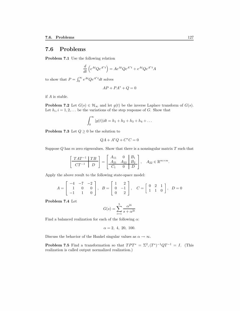
7.6. Problems 127
7.6 Problems
Problem 7.1 Use the following relation
d
dt
(eAtQeA
∗t)
= AeAtQeA∗t + eAtQeA
∗tA
to show that P =∫∞
0 eAtQeA∗tdt solves
AP + PA∗ +Q = 0
if A is stable.
Problem 7.2 Let G(s) ∈ H∞ and let g(t) be the inverse Laplace transform of G(s).Let hi, i = 1, 2, . . . be the variations of the step response of G. Show that∫ ∞
0
|g(t)|dt = h1 + h2 + h3 + h4 + . . .
Problem 7.3 Let Q ≥ 0 be the solution to
QA+A∗Q+ C∗C = 0
Suppose Q has m zero eigenvalues. Show that there is a nonsingular matrix T such that[TAT−1 TB
CT−1 D
]=
A11 0 B1
A21 A22 B2
C1 0 D
, A22 ∈ Rm×m.
Apply the above result to the following state-space model:
A =
−4 −7 −21 0 0−1 1 0
, B =
1 20 −10 2
, C =[
0 2 11 1 0
], D = 0
Problem 7.4 Let
G(s) =5∑i=1
α2i
s+ α2i
Find a balanced realization for each of the following α:
α = 2, 4, 20, 100.
Discuss the behavior of the Hankel singular values as α→∞.
Problem 7.5 Find a transformation so that TPT ∗ = Σ2, (T ∗)−1QT−1 = I. (Thisrealization is called output normalized realization.)

128 BALANCED MODEL REDUCTION
Problem 7.6 Consider the model reduction error:
E11 =
A11 0 A12/2 B1
0 A11 −A12/2 0A21 −A21 A22 B2
0 −2C1 C2 0
=:[Ae BeCe 0
].
Show that
P =
Σ1 00 σ2
NΣ−11 0
0 0 2σNIsN
satisfies
AeP + PA∗e +BeB∗e +
14σ2
N
PC∗eCeP = 0.
Problem 7.7 Suppose P and Q are the controllability and observability Gramians ofG(s) = C(sI − A)−1B ∈ RH∞. Let Gd(z) = G(s)|s= z+1
z−1= Cd(zI − Ad)−1Bd + Dd.
Compute the controllability and observability Gramians Pd and Qd and compare PQand PdQd.
Problem 7.8 Note that a delay can be approximated as
e−τs ≈(
1− τ2ns
1 + τ2ns
)n
for a sufficiently large n. Let a process modele−s
1 + Tsbe approximated by
G(s) =(
1− 0.05s1 + 0.05s
)10 11 + sT
For each T = 0, 0.01, 0.1, 1, 10, find a reduced-order model, if possible, using balancedtruncation such that the approximation error is no greater than 0.1.

Chapter 8
Uncertainty and Robustness
In this chapter we briefly describe various types of uncertainties that can arise in phys-ical systems, and we single out “unstructured uncertainties” as generic errors that areassociated with all design models. We obtain robust stability tests for systems undervarious model uncertainty assumptions through the use of the small gain theorem. Wealso obtain some sufficient conditions for robust performance under unstructured un-certainties. The difficulty associated with MIMO robust performance design and therole of plant condition numbers for systems with skewed performance and uncertaintyspecifications are revealed. A simple example is also used to indicate the fundamentaldifference between the robustness of an SISO system and that of a MIMO system. Inparticular, we show that applying the SISO analysis/design method to a MIMO systemmay lead to erroneous results.
8.1 Model Uncertainty
Most control designs are based on the use of a design model. The relationship betweenmodels and the reality they represent is subtle and complex. A mathematical modelprovides a map from inputs to responses. The quality of a model depends on how closelyits responses match those of the true plant. Since no single fixed model can respondexactly like the true plant, we need, at the very least, a set of maps. However, themodeling problem is much deeper — the universe of mathematical models from which amodel set is chosen is distinct from the universe of physical systems. Therefore, a modelset that includes the true physical plant can never be constructed. It is necessary forthe engineer to make a leap of faith regarding the applicability of a particular designbased on a mathematical model. To be practical, a design technique must help makethis leap small by accounting for the inevitable inadequacy of models. A good modelshould be simple enough to facilitate design, yet complex enough to give the engineerconfidence that designs based on the model will work on the true plant.
The term uncertainty refers to the differences or errors between models and reality,
129

130 UNCERTAINTY AND ROBUSTNESS
and whatever mechanism is used to express these errors will be called a representationof uncertainty. Representations of uncertainty vary primarily in terms of the amountof structure they contain. This reflects both our knowledge of the physical mechanismsthat cause differences between the model and the plant and our ability to represent thesemechanisms in a way that facilitates convenient manipulation. For example, considerthe problem of bounding the magnitude of the effect of some uncertainty on the outputof a nominally fixed linear system. A useful measure of uncertainty in this context isto provide a bound on the power spectrum of the output’s deviation from its nominalresponse. In the simplest case, this power spectrum is assumed to be independentof the input. This is equivalent to assuming that the uncertainty is generated by anadditive noise signal with a bounded power spectrum; the uncertainty is represented asadditive noise. Of course, no physical system is linear with additive noise, but someaspects of physical behavior are approximated quite well using this model. This typeof uncertainty received a great deal of attention in the literature during the 1960s and1970s, and elegant solutions are obtained for many interesting problems (e.g., whitenoise propagation in linear systems, Wiener and Kalman filtering, and LQG optimalcontrol). Unfortunately, LQG optimal control did not address uncertainty adequatelyand hence had less practical impact than might have been hoped.
Generally, the deviation’s power spectrum of the true output from the nominal willdepend significantly on the input. For example, an additive noise model is entirely in-appropriate for capturing uncertainty arising from variations in the material propertiesof physical plants. The actual construction of model sets for more general uncertaintycan be quite difficult. For example, a set membership statement for the parameters ofan otherwise known FDLTI model is a highly structured representation of uncertainty.It typically arises from the use of linear incremental models at various operating points(e.g., aerodynamic coefficients in flight control vary with flight environment and air-craft configurations, and equation coefficients in power plant control vary with aging,slag buildup, coal composition, etc.). In each case, the amounts of variation and anyknown relationships between parameters can be expressed by confining the parametersto appropriately defined subsets of parameter space. However, for certain classes of sig-nals (e.g., high-frequency), the parameterized FDLTI model fails to describe the plantbecause the plant will always have dynamics that are not represented in the fixed ordermodel.
In general, we are forced to use not just a single parameterized model but model setsthat allow for plant dynamics that are not explicitly represented in the model struc-ture. A simple example of this involves using frequency domain bounds on transferfunctions to describe a model set. To use such sets to describe physical systems, thebounds must roughly grow with frequency. In particular, at sufficiently high frequencies,phase is completely unknown (i.e., ±180o uncertainties). This is a consequence of dy-namic properties that inevitably occur in physical systems. This gives a less structuredrepresentation of uncertainty.

8.1. Model Uncertainty 131
Examples of less structured representations of uncertainty are direct set membershipstatements for the transfer function matrix of the model. For instance, the statement
P∆(s) = P (s) +W1(s)∆(s)W2(s), σ[∆(jω)] < 1, ∀ω ≥ 0, (8.1)
whereW1 andW2 are stable transfer matrices that characterize the spatial and frequencystructure of the uncertainty, confines the matrix P∆ to a neighborhood of the nominalmodel P . In particular, if W1 = I and W2 = w(s)I, where w(s) is a scalar function,then P∆ describes a disk centered at P with radius w(jω) at each frequency, as shown inFigure 8.1. The statement does not imply a mechanism or structure that gives rise to ∆.The uncertainty may be caused by parameter changes, as mentioned previously or byneglected dynamics, or by a host of other unspecified effects. An alternative statementto equation (8.1) is the so-called multiplicative form:
P∆(s) = (I +W1(s)∆(s)W2(s))P (s). (8.2)
This statement confines P∆ to a normalized neighborhood of the nominal model P . Anadvantage of equation (8.2) over (8.1) is that in equation (8.2) compensated transferfunctions have the same uncertainty representation as the raw model (i.e., the weightingfunctions apply to PK as well as P ). Some other alternative set membership statementswill be discussed later.
P(j
w(jω
ω )
)
Figure 8.1: Nyquist diagram of an uncertain model
The best choice of uncertainty representation for a specific FDLTI model depends,of course, on the errors the model makes. In practice, it is generally possible to repre-sent some of these errors in a highly structured parameterized form. These are usuallythe low-frequency error components. There are always remaining higher-frequency er-rors, however, which cannot be covered this way. These are caused by such effects asinfinite-dimensional electromechanical resonance, time delays, diffusion processes, etc.Fortunately, the less structured representations, such as equations (8.1) and (8.2), arewell suited to represent this latter class of errors. Consequently, equations (8.1) and

132 UNCERTAINTY AND ROBUSTNESS
(8.2) have become widely used “generic” uncertainty representations for FDLTI models.An important point is that the construction of the weighting matrices W1 and W2 formultivariable systems is not trivial.
Motivated from these observations, we will focus for the moment on the multiplica-tive description of uncertainty. We will assume that P∆ in equation (8.2) remains astrictly proper FDLTI system for all ∆. More general perturbations (e.g., time varying,infinite dimensional, nonlinear) can also be covered by this set provided they are givenappropriate “conic sector” interpretations via Parseval’s theorem. This connection isdeveloped in [Safonov, 1980] and [Zames, 1966] and will not be pursued here.
When used to represent the various high-frequency mechanisms mentioned previ-ously, the weighting functions in equation (8.2) commonly have the properties illustratedin Figure 8.2. They are small ( 1) at low frequencies and increase to unity and aboveat higher frequencies. The growth with frequency inevitably occurs because phase un-certainties eventually exceed ±180 degrees and magnitude deviations eventually exceedthe nominal transfer function magnitudes. Readers who are skeptical about this realityare encouraged to try a few experiments with physical devices.
actual model
log
nominal model
ω
Figure 8.2: Typical behavior of multiplicative uncertainty: pδ(s) = [1 + w(s)δ(s)]p(s)
Also note that the representation of uncertainty in equation (8.2) can be used toinclude perturbation effects that are in fact certain. A nonlinear element may be quiteaccurately modeled, but because our design techniques cannot effectively deal with thenonlinearity, it is treated as a conic sector nonlinearity.1 As another example, we maydeliberately choose to ignore various known dynamic characteristics in order to achievea simple nominal design model. One such instance is the model reduction processdiscussed in the last chapter.
1See, for example, Safonov [1980] and Zames [1966].

8.1. Model Uncertainty 133
Example 8.1 Let a dynamical system be described by
P (s, α, β) =10((2 + 0.2α)s2 + (2 + 0.3α+ 0.4β)s+ (1 + 0.2β)
)(s2 + 0.5s+ 1)(s2 + 2s+ 3)(s2 + 3s+ 6)
, α, β ∈ [−1, 1]
Then for each frequency, all possible frequency responses with varying parameters α andβ are in a box, as shown in Figure 8.3. We can also obtain an unstructured uncertaintybound for this system. In fact, we have
P (s, α, β) ∈ P0 +W∆ | ‖∆‖ ≤ 1
with P0 := P (s, 0, 0) and
W (s) = P (s, 1, 1)− P (s, 0, 0) =10(0.2s2 + 0.7s+ 0.2
)(s2 + 0.5s+ 1)(s2 + 2s+ 3)(s2 + 3s+ 6)
The frequency response P0 +W∆ is shown in Figure 8.3 as circles.
−2 −1.5 −1 −0.5 0 0.5 1 1.5 2 2.5−3.5
−3
−2.5
−2
−1.5
−1
−0.5
0
0.5
Figure 8.3: Nyquist diagram of uncertain system and disk covering
Another way to bound the frequency response is to treat α and β as norm boundeduncertainties; that is,
P (s, α, β) ∈ P0 +W1∆1 +W2∆2 | ‖∆i‖∞ ≤ 1
with P0 = P (s, 0, 0) and
W1 =10(0.2s2 + 0.3s)
(s2 + 0.5s+ 1)(s2 + 2s+ 3)(s2 + 3s+ 6),

134 UNCERTAINTY AND ROBUSTNESS
W2 =10(0.4s+ 0.2)
(s2 + 0.5s+ 1)(s2 + 2s+ 3)(s2 + 3s+ 6)It is in fact easy to show that
P0 +W1∆1 +W2∆2 | ‖∆i‖∞ ≤ 1 = P0 +W∆ | ‖∆‖∞ ≤ 1
with |W | = |W1|+ |W2|. The frequency response P0 +W∆ is shown in Figure 8.4. Thisbounding is clearly more conservative.
−2 −1.5 −1 −0.5 0 0.5 1 1.5 2 2.5−3.5
−3
−2.5
−2
−1.5
−1
−0.5
0
0.5
1
Figure 8.4: A conservative covering
Example 8.2 Consider a process control model
G(s) =ke−τs
Ts+ 1, 4 ≤ k ≤ 9, 2 ≤ T ≤ 3, 1 ≤ τ ≤ 2.
Take the nominal model as
G0(s) =6.5
(2.5s+ 1)(1.5s+ 1)
Then for each frequency, all possible frequency responses are in a box, as shown inFigure 8.5. To obtain an unstructured uncertainty bound for this system, plot the error
∆a(jω) = G(jω)−G0(jω)
for a set of parameters, as shown in Figure 8.6, and then use the Matlab commandginput to pick a set of upper-bound frequency responses and use fitmag to fit a stableand minimum phase transfer function to the upper-bound frequency responses.

8.1. Model Uncertainty 135
−5 0 5 10−8
−6
−4
−2
0
2
4
ω = 0.01ω = 0.01
ω = 0.05
ω = 0.01
ω = 0.05
ω = 0.1
ω = 0.01
ω = 0.05
ω = 0.1
ω = 0.2
ω = 0.01
ω = 0.05
ω = 0.1
ω = 0.2
ω = 0.3
ω = 0.01
ω = 0.05
ω = 0.1
ω = 0.2
ω = 0.3ω = 0.5
ω = 0.01
ω = 0.05
ω = 0.1
ω = 0.2
ω = 0.3ω = 0.5
ω = 0.8
ω = 0.01
ω = 0.05
ω = 0.1
ω = 0.2
ω = 0.3ω = 0.5
ω = 0.8
ω = 1ω = 0.01
ω = 0.05
ω = 0.1
ω = 0.2
ω = 0.3ω = 0.5
ω = 0.8
ω = 1
ω = 2
ω = 0.01
ω = 0.05
ω = 0.1
ω = 0.2
ω = 0.3ω = 0.5
ω = 0.8
ω = 1
ω = 2
ω = 3
Real
Imag
inar
y
Figure 8.5: Uncertain delay system and G0
mf= ginput(50) % pick 50 points: the first column of mf is the frequency pointsand the second column of mf is the corresponding magnitude responses.
magg=vpck(mf(:,2),mf(:,1)); % pack them as a varying matrix.
Wa =fitmag(magg); % choose the order of Wa online. A third-order Wa issufficient for this example.
[A,B,C,D]=unpck(Wa) % converting into state-space.
[Z, P, K]=ss2zp(A,B,C,D) % converting into zero/pole/gain form.
We get
Wa(s) =0.0376(s+ 116.4808)(s+ 7.4514)(s+ 0.2674)
(s+ 1.2436)(s+ 0.5575)(s+ 4.9508)
and the frequency response of Wa is also plotted in Figure 8.6. Similarly, define themultiplicative uncertainty
∆m(s) :=G(s)−G0(s)
G0(s)
and a Wm can be found such that |∆m(jω)| ≤ |Wm(jω)|, as shown in Figure 8.7. AWm is given by
Wm =2.8169(s+ 0.212)(s2 + 2.6128s+ 1.732)
s2 + 2.2425s+ 2.6319

136 UNCERTAINTY AND ROBUSTNESS
10−2
10−1
100
101
102
10−2
10−1
100
101
Figure 8.6: ∆a (dashed line) and a bound Wa (solid line)
10−2
10−1
100
101
102
10−5
10−4
10−3
10−2
10−1
100
101
102
103
Figure 8.7: ∆m (dashed line) and a bound Wm (solid line)

8.2. Small Gain Theorem 137
Note that this Wm is not proper since G0 and G do not have the same relative degrees.To get a proper Wm, we need to choose a nominal model G0 having the same the relativeorder as that of G.
The following terminologies are used in this book:
Definition 8.1 Given the description of an uncertainty model set Π and a set of per-formance objectives, suppose P ∈Π is the nominal design model and K is the resultingcontroller. Then the closed-loop feedback system is said to have
Nominal Stability (NS): if K internally stabilizes the nominal model P .
Robust Stability (RS): if K internally stabilizes every plant belonging to Π.
Nominal Performance (NP): if the performance objectives are satisfied for thenominal plant P .
Robust Performance (RP): if the performance objectives are satisfied for everyplant belonging to Π.
The nominal stability and performance can be easily checked using various standardtechniques. The conditions for which the robust stability and robust performance aresatisfied under various assumptions on the uncertainty set Π will be considered in thefollowing sections.
Related MATLAB Commands: magfit, drawmag, fitsys, genphase, vunpck,vabs, vinv, vimag, vreal, vcjt, vebe
8.2 Small Gain Theorem
This section and the next section consider the stability test of a nominally stable systemunder unstructured perturbations. The basis for the robust stability criteria derived inthe sequel is the so-called small gain theorem.
Consider the interconnected system shown in Figure 8.8 with M(s) a stable p × qtransfer matrix.
Theorem 8.1 (Small Gain Theorem) Suppose M ∈ RH∞ and let γ > 0. Then theinterconnected system shown in Figure 8.8 is well-posed and internally stable for all∆(s) ∈ RH∞ with
(a) ‖∆‖∞ ≤ 1/γ if and only if ‖M(s)‖∞ < γ
(b) ‖∆‖∞ < 1/γ if and only if ‖M(s)‖∞ ≤ γ

138 UNCERTAINTY AND ROBUSTNESS
ee
++
++e2
e1
w2
w1
-6
?
-
M
∆
Figure 8.8: M −∆ loop for stability analysis
Proof. We shall only prove part (a). The proof for part (b) is similar. Without lossof generality, assume γ = 1.
(Sufficiency) It is clear that M(s)∆(s) is stable since both M(s) and ∆(s) are stable.Thus by Theorem 5.5 (or Corollary 5.4) the closed-loop system is stable if det(I−M∆)has no zero in the closed right-half plane for all ∆ ∈ RH∞ and ‖∆‖∞ ≤ 1. Equivalently,the closed-loop system is stable if
infs∈C+
σ (I −M(s)∆(s)) 6= 0
for all ∆ ∈ RH∞ and ‖∆‖∞ ≤ 1. But this follows from
infs∈C+
σ (I −M(s)∆(s)) ≥ 1− sups∈C+
σ (M(s)∆(s)) = 1−‖M(s)∆(s)‖∞ ≥ 1−‖M(s)‖∞ > 0.
(Necessity) This will be shown by contradiction. Suppose ‖M‖∞ ≥ 1. We will showthat there exists a ∆ ∈ RH∞ with ‖∆‖∞ ≤ 1 such that det(I −M(s)∆(s)) has azero on the imaginary axis, so the system is unstable. Suppose ω0 ∈ R+ ∪ ∞ issuch that σ(M(jω0)) ≥ 1. Let M(jω0) = U(jω0)Σ(jω0)V ∗(jω0) be a singular valuedecomposition with
U(jω0) =[u1 u2 · · · up
]V (jω0) =
[v1 v2 · · · vq
]Σ(jω0) =
σ1
σ2
. . .
To obtain a contradiction, it now suffices to construct a ∆ ∈ RH∞ such that ∆(jω0) =1σ1v1u∗1 and ‖∆‖∞ ≤ 1. Indeed, for such ∆(s),
det(I −M(jω0)∆(jω0)) = det(I − UΣV ∗v1u∗1/σ1) = 1− u∗1UΣV ∗v1/σ1 = 0
and thus the closed-loop system is either not well-posed (if ω0 = ∞) or unstable (ifω ∈ R). There are two different cases:
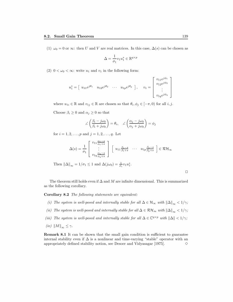
8.2. Small Gain Theorem 139
(1) ω0 = 0 or∞: then U and V are real matrices. In this case, ∆(s) can be chosen as
∆ =1σ1v1u∗1 ∈ Rq×p
(2) 0 < ω0 <∞: write u1 and v1 in the following form:
u∗1 =[u11e
jθ1 u12ejθ2 · · · u1pe
jθp], v1 =
v11e
jφ1
v12ejφ2
...v1qe
jφq
where u1i ∈ R and v1j ∈ R are chosen so that θi, φj ∈ [−π, 0) for all i, j.
Choose βi ≥ 0 and αj ≥ 0 so that
∠(βi − jω0
βi + jω0
)= θi, ∠
(αj − jω0
αj + jω0
)= φj
for i = 1, 2, . . . , p and j = 1, 2, . . . , q. Let
∆(s) =1σ1
v11α1−sα1+s...
v1qαq−sαq+s
[ u11β1−sβ1+s · · · u1p
βp−sβp+s
]∈ RH∞
Then ‖∆‖∞ = 1/σ1 ≤ 1 and ∆(jω0) = 1σ1v1u∗1.
2
The theorem still holds even if ∆ and M are infinite dimensional. This is summarizedas the following corollary.
Corollary 8.2 The following statements are equivalent:
(i) The system is well-posed and internally stable for all ∆ ∈ H∞ with ‖∆‖∞ < 1/γ;
(ii) The system is well-posed and internally stable for all ∆ ∈ RH∞ with ‖∆‖∞ < 1/γ;
(iii) The system is well-posed and internally stable for all ∆ ∈ Cq×p with ‖∆‖ < 1/γ;
(iv) ‖M‖∞ ≤ γ.
Remark 8.1 It can be shown that the small gain condition is sufficient to guaranteeinternal stability even if ∆ is a nonlinear and time-varying “stable” operator with anappropriately defined stability notion, see Desoer and Vidyasagar [1975]. 3

140 UNCERTAINTY AND ROBUSTNESS
The following lemma shows that if ‖M‖∞ > γ, there exists a destabilizing ∆ with‖∆‖∞ < 1/γ such that the closed-loop system has poles in the open right-half plane.(This is stronger than what is given in the proof of Theorem 8.1.)
Lemma 8.3 Suppose M ∈ RH∞ and ‖M‖∞ > γ. Then there exists a σ0 > 0 suchthat for any given σ ∈ [0, σ0] there exists a ∆ ∈ RH∞ with ‖∆‖∞ < 1/γ such thatdet(I −M(s)∆(s)) has a zero on the axis Re(s) = σ.
Proof. Without loss of generality, assume γ = 1. Since M ∈ RH∞ and‖M‖∞ > 1, there exists a 0 < ω0 <∞ such that ‖M(jω0)‖ > 1. Given any γ such that1 < γ < ‖M(jω0)‖, there is a sufficiently small σ0 > 0 such that
minσ∈[0,σ0]
‖M(σ + jω0)‖ ≥ γ
and √ω2
0 + (σ0 + α)2
ω20 + (σ0 − α)2
√ω2
0 + (σ0 + β)2
ω20 + (σ0 − β)2
< γ
for any α ≥ 0 and β ≥ 0.Now let σ ∈ [0, σ0] and let M(σ + jω0) = UΣV ∗ be a singular value decomposition
withU =
[u1 u2 · · · up
]V =
[v1 v2 · · · vq
]Σ =
σ1
σ2
. . .
.Write u1 and v1 in the following form:
u∗1 =[u11e
jθ1 u12ejθ2 · · · u1pe
jθp], v1 =
v11e
jφ1
v12ejφ2
...v1qe
jφq
where u1i ∈ R and v1j ∈ R are chosen so that θi, φj ∈ [−π, 0) for all i, j.
Choose βi ≥ 0 and αj ≥ 0 so that
∠(βi − σ − jω0
βi + σ + jω0
)= θi, ∠
(αj − σ − jω0
αj + σ + jω0
)= φj
for i = 1, 2, . . . , p and j = 1, 2, . . . , q. Let
∆(s) =1σ1
α1v11α1−sα1+s
...αqv1q
αq−sαq+s
[ β1u11β1−sβ1+s · · · βpu1p
βp−sβp+s
]∈ RH∞

8.3. Stability under Unstructured Uncertainties 141
where
βi :=
√ω2
0 + (σ + βi)2
ω20 + (σ − βi)2
, αj :=
√ω2
0 + (σ + αj)2
ω20 + (σ − αj)2
Then
‖∆‖∞ ≤maxj αjmaxi
βi
σ1≤
maxj αjmaxiβi
γ< 1
and∆(σ + jω0) =
1σ1v1u∗1
det (I −M(σ + jω0)∆(σ + jω0)) = 0
Hence s = σ + jω0 is a zero for the transfer function det (I −M(s)∆(s)). 2
The preceding lemma plays a key role in the necessity proofs of many robust stabilitytests in the sequel.
8.3 Stability under Unstructured Uncertainties
The small gain theorem in the last section will be used here to derive robust stabilitytests under various assumptions of model uncertainties. The modeling error ∆ will againbe assumed to be stable. (Most of the robust stability tests discussed in the sequel canbe generalized easily to the unstable ∆ case with some mild assumptions on the numberof unstable poles of the uncertain model; we encourage readers to fill in the details.)In addition, we assume that the modeling error ∆ is suitably scaled with weightingfunctions W1 and W2 (i.e., the uncertainty can be represented as W1∆W2).
f K Π- - -6
-
−
Figure 8.9: Unstructured robust stability analysis
We shall consider the standard setup shown in Figure 8.9, where Π is the set of un-certain plants with P ∈Π as the nominal plant and with K as the internally stabilizingcontroller for P . The sensitivity and complementary sensitivity matrix functions aredefined, as usual, as
So = (I + PK)−1, To = I − Soand
Si = (I +KP )−1, Ti = I − Si.

142 UNCERTAINTY AND ROBUSTNESS
Recall that the closed-loop system is well-posed and internally stable if and only if[I K−Π I
]−1
=[
(I +KΠ)−1 −K(I + ΠK)−1
(I + ΠK)−1Π (I + ΠK)−1
]∈ RH∞
for all Π ∈Π.
8.3.1 Additive Uncertainty
We assume that the model uncertainty can be represented by an additive perturbation:
Π = P +W1∆W2.
Theorem 8.4 Let Π = P +W1∆W2 : ∆ ∈ RH∞ and let K be a stabilizing con-troller for the nominal plant P . Then the closed-loop system is well-posed and internallystable for all ‖∆‖∞ < 1 if and only if ‖W2KSoW1‖∞ ≤ 1.
Proof. Let Π = P +W1∆W2 ∈Π. Then[I K−Π I
]−1
=[
(I +KSoW1∆W2)−1Si −KSo(I +W1∆W2KSo)−1
(I + SoW1∆W2K)−1So(P +W1∆W2) So(I +W1∆W2KSo)−1
]is well-posed and internally stable if (I + ∆W2KSoW1)−1 ∈ RH∞ since
det(I +KSoW1∆W2) = det(I +W1∆W2KSo) = det(I + SoW1∆W2K)= det(I + ∆W2KSoW1).
But (I + ∆W2KSoW1)−1 ∈ RH∞ is guaranteed if ‖∆W2KSoW1‖∞ < 1 (small gaintheorem). Hence ‖W2KSoW1‖∞ ≤ 1 is sufficient for robust stability.
To show the necessity, note that robust stability implies that
K(I + ΠK)−1 = KSo(I +W1∆W2KSo)−1 ∈ RH∞
for all admissible ∆. This, in turn, implies that
∆W2K(I + ΠK)−1W1 = I − (I + ∆W2KSoW1)−1 ∈ RH∞
for all admissible ∆. By the small gain theorem, this is true for all ∆ ∈ RH∞ with‖∆‖∞ < 1 only if ‖W2KSoW1‖∞ ≤ 1. 2

8.3. Stability under Unstructured Uncertainties 143
e eee-dm
?wz
6
-
?
--
-----
W2 ∆ W1
Pey
d
d
−
r ?
?Wd
-We-K
Figure 8.10: Output multiplicative perturbed systems
8.3.2 Multiplicative Uncertainty
In this section, we assume that the system model is described by the following set ofmultiplicative perturbations:
Π = (I +W1∆W2)P
with W1,W2,∆ ∈ RH∞. Consider the feedback system shown in Figure 8.10.
Theorem 8.5 Let Π = (I +W1∆W2)P : ∆ ∈ RH∞ and let K be a stabilizing con-troller for the nominal plant P . Then the closed-loop system is well-posed and internallystable for all ∆ ∈ RH∞ with ‖∆‖∞ < 1 if and only if ‖W2ToW1‖∞ ≤ 1.
Proof. We shall first prove that the condition is necessary for robust stability. Suppose‖W2ToW1‖∞ > 1. Then by Lemma 8.3, for any given sufficiently small σ > 0, thereis a ∆ ∈ RH∞ with ‖∆‖∞ < 1 such that (I + ∆W2ToW1)−1 has poles on the axisRe(s) = σ. This implies that
(I + ΠK)−1 = So(I +W1∆W2To)−1
has poles on the axis Re(s) = σ since σ can always be chosen so that the unstable polesare not cancelled by the zeros of So. Hence ‖W2ToW1‖∞ ≤ 1 is necessary for robuststability. The sufficiency follows from the small gain theorem. 2

144 UNCERTAINTY AND ROBUSTNESS
8.3.3 Coprime Factor Uncertainty
As another example, consider a left coprime factor perturbed plant described in Fig-ure 8.11.
eee
−
−
yw
z2z1
r
6
?
-
∆M
M−1--
-
N
∆N-
-K--
Figure 8.11: Left coprime factor perturbed systems
Theorem 8.6 LetΠ = (M + ∆M )−1(N + ∆N )
with M, N, ∆M , ∆N ∈ RH∞. The transfer matrices (M, N) are assumed to be a stableleft coprime factorization of P (i.e., P = M−1N), and K internally stabilizes thenominal system P . Define ∆ :=
[∆N ∆M
]. Then the closed-loop system is well-
posed and internally stable for all ‖∆‖∞ < 1 if and only if∥∥∥∥[ KI
](I + PK)−1M−1
∥∥∥∥∞≤ 1
Proof. Let K = UV −1 be a right coprime factorization over RH∞. By Lemma 5.7,the closed-loop system is internally stable if and only if(
(N + ∆N )U + (M + ∆M )V)−1
∈ RH∞ (8.3)
Since K stabilizes P , (NU + MV )−1 ∈ RH∞. Hence equation (8.3) holds if and only if(I + (∆NU + ∆MV )(NU + MV )−1
)−1
∈ RH∞
By the small gain theorem, the above is true for all ‖∆‖∞ < 1 if and only if∥∥∥∥[ UV
](NU + MV )−1
∥∥∥∥∞
=∥∥∥∥[ K
I
](I + PK)−1M−1
∥∥∥∥∞≤ 1
2

8.3. Stability under Unstructured Uncertainties 145
8.3.4 Unstructured Robust Stability Tests
Table 8.1 summaries robust stability tests on the plant uncertainties under variousassumptions. All of the tests pertain to the standard setup shown in Figure 8.9, whereΠ is the set of uncertain plants with P ∈ Π as the nominal plant and with K as theinternally stabilizing controller of P .
W1 ∈ RH∞ W2 ∈ RH∞ ∆ ∈ RH∞ ‖∆‖∞ < 1
Perturbed Model Sets Representative Types of Robust Stability TestsΠ Uncertainty Characterized
output (sensor) errors(I +W1∆W2)P neglected HF dynamics ‖W2ToW1‖∞ ≤ 1
uncertain rhp zerosinput (actuators) errors
P (I +W1∆W2) neglected HF dynamics ‖W2TiW1‖∞ ≤ 1uncertain rhp zerosLF parameter errors
(I +W1∆W2)−1P uncertain rhp poles ‖W2SoW1‖∞ ≤ 1
LF parameter errorsP (I +W1∆W2)−1 uncertain rhp poles ‖W2SiW1‖∞ ≤ 1
additive plant errorsP +W1∆W2 neglected HF dynamics ‖W2KSoW1‖∞ ≤ 1
uncertain rhp zerosLF parameter errors
P (I +W1∆W2P )−1 uncertain rhp poles ‖W2SoPW1‖∞ ≤ 1
(M + ∆M )−1(N + ∆N ) LF parameter errors
P = M−1N neglected HF dynamics∥∥∥∥[ K
I
]SoM
−1
∥∥∥∥∞≤ 1
∆ =[
∆N ∆M
]uncertain rhp poles & zeros
(N + ∆N )(M + ∆M )−1 LF parameter errorsP = NM−1 neglected HF dynamics
∥∥M−1Si[K I]∥∥∞ ≤ 1
∆ =[
∆N
∆M
]uncertain rhp poles & zeros
Table 8.1: Unstructured robust stability tests (HF: high frequency, LF: low frequency)

146 UNCERTAINTY AND ROBUSTNESS
Table 8.1 should be interpreted as follows:
UNSTRUCTURED ANALYSIS THEOREM
Given NS & Perturbed Model Sets
Then Closed-Loop Robust Stability
if and only if Robust Stability Tests
The table also indicates representative types of physical uncertainties that can beusefully represented by cone-bounded perturbations inserted at appropriate locations.For example, the representation P∆ = (I +W1∆W2)P in the first row is useful for out-put errors at high frequencies (HF), covering such things as unmodeled high-frequencydynamics of sensors or plants, including diffusion processes, transport lags, electrome-chanical resonances, etc. The representation P∆ = P (I + W1∆W2) in the second rowcovers similar types of errors at the inputs. Both cases should be contrasted withthe third and the fourth rows, which treat P (I + W1∆W2)−1 and (I + W1∆W2)−1P .These representations are more useful for variations in modeled dynamics, such as low-frequency (LF) errors produced by parameter variations with operating conditions, withaging, or across production copies of the same plant.
Note from the table that the stability requirements on ∆ do not limit our abilityto represent variations in either the number or locations of rhp singularities, as can beseen from some simple examples.
Example 8.3 Suppose an uncertain system with changing numbers of right-half planepoles is described by
P∆ =
1s− δ : δ ∈ R, |δ| ≤ 1
.
Then P1 =1
s− 1∈ P∆ has one right-half plane pole and P2 =
1s+ 1
∈ P∆ has no
right-half plane pole. Nevertheless, the set of P∆ can be covered by a set of feedbackuncertain plants:
P∆ ⊂Π :=P (1 + δP )−1 : δ ∈ RH∞, ‖δ‖∞ ≤ 1
with P =
1s
.

8.4. Robust Performance 147
Example 8.4 As another example, consider the following set of plants:
P∆ =s+ 1 + α
(s+ 1)(s+ 2), |α| ≤ 2.
This set of plants has changing numbers of right-half plane zeros since the plant has noright-half plane zero when α = 0 and has one right-half plane zero when α = −2. Theuncertain plant can be covered by a set of multiplicative perturbed plants:
P∆ ⊂ Π :=
1s+ 2
(1 +2δs+ 1
), δ ∈ RH∞, ‖δ‖∞ ≤ 1.
It should be noted that this covering can be quite conservative.
8.4 Robust Performance
Consider the perturbed system shown in Figure 8.12 with the set of perturbed modelsdescribed by a set Π. Suppose the weighting matrices Wd,We ∈ RH∞ and the perfor-
e e- P∆ ∈Π6
- - eyd
d
−
r ?
?Wd
-We--K
Figure 8.12: Diagram for robust performance analysis
mance criterion is to keep the error e as small as possible in some sense for all possiblemodels belonging to the set Π. In general, the set Π can be either a parameterized setor an unstructured set such as those described in Table 8.1. The performance specifica-tions are usually specified in terms of the magnitude of each component e in the timedomain with respect to bounded disturbances, or, alternatively and more conveniently,some requirements on the closed-loop frequency response of the transfer matrix betweend and e (say, integral of square error or the magnitude of the steady-state error withrespect to sinusoidal disturbances). The former design criterion leads to the so-called

148 UNCERTAINTY AND ROBUSTNESS
L1-optimal control framework and the latter leads to H2 and H∞ design frameworks,respectively. In this section, we will focus primarily on the H∞ performance objectiveswith unstructured model uncertainty descriptions. The performance under structureduncertainty will be considered in Chapter 10.
Suppose the performance criterion is to keep the worst-case energy of the error e assmall as possible over all d of unit energy, for example,
sup‖d‖2
≤1
‖e‖2 ≤ ε
for some small ε. By scaling the error e (i.e., by properly selecting We) we can assumewithout loss of generality that ε = 1.
Let Ted denote the transfer matrix between d and e, then
Ted = We(I + P∆K)−1Wd, P∆ ∈ Π. (8.4)
Then the robust performance criterion in this case can be described as requiring thatthe closed-loop system be robustly stable and that∥∥Ted∥∥∞ ≤ 1, ∀P∆ ∈ Π. (8.5)
More specifically, an output multiplicatively perturbed system will be analyzed first.The analysis for other classes of models can be done analogously. The perturbed modelcan be described as
Π := (I +W1∆W2)P : ∆ ∈ RH∞, ‖∆‖∞ < 1 (8.6)
with W1,W2 ∈ RH∞. The explicit system diagram is as shown in Figure 8.10. For thisclass of models, we have
Ted = WeSo(I +W1∆W2To)−1Wd,
and the robust performance is satisfied iff
‖W2ToW1‖∞ ≤ 1
and ∥∥Ted∥∥∞ ≤ 1, ∀∆ ∈ RH∞, ‖∆‖∞ < 1.
The exact analysis for this robust performance problem is not trivial and will be givenin Chapter 10. However, some sufficient conditions are relatively easy to obtain bybounding these two inequalities, and they may shed some light on the nature of theseproblems. It will be assumed throughout that the controller K internally stabilizes thenominal plant P .
Theorem 8.7 Suppose P∆ ∈ (I +W1∆W2)P : ∆ ∈ RH∞, ‖∆‖∞ < 1 and K in-ternally stabilizes P . Then the system robust performance is guaranteed if either one ofthe following conditions is satisfied:

8.4. Robust Performance 149
(i) for each frequency ω
σ(Wd)σ(WeSo) + σ(W1)σ(W2To) ≤ 1; (8.7)
(ii) for each frequency ω
κ(W−11 Wd)σ(WeSoWd) + σ(W2ToW1) ≤ 1 (8.8)
where W1 and Wd are assumed to be invertible and κ(W−11 Wd) is the condition
number.
Proof. It is obvious that both condition (8.7) and condition (8.8) guarantee that‖W2ToW1‖∞ ≤ 1. So it is sufficient to show that
∥∥Ted∥∥∞ ≤ 1,∀∆ ∈ RH∞, ‖∆‖∞ < 1.Now for any frequency ω, it is easy to see that
σ(Ted) ≤ σ(WeSo)σ[(I +W1∆W2To)−1]σ(Wd)
=σ(WeSo)σ(Wd)σ(I +W1∆W2To)
≤ σ(WeSo)σ(Wd)1− σ(W1∆W2To)
≤ σ(WeSo)σ(Wd)1− σ(W1)σ(W2To)σ(∆)
.
Hence condition (8.7) guarantees σ(Ted) ≤ 1 for all ∆ ∈ RH∞ with ‖∆‖∞ < 1 at allfrequencies.
Similarly, suppose W1 and Wd are invertible; write
Ted = WeSoWd(W−11 Wd)−1(I + ∆W2ToW1)−1(W−1
1 Wd),
and then
σ(Ted) ≤σ(WeSoWd)κ(W−1
1 Wd)1− σ(W2ToW1)σ(∆)
.
Hence by condition (8.8), σ(Ted) ≤ 1 is guaranteed for all ∆ ∈ RH∞ with ‖∆‖∞ < 1at all frequencies. 2
Remark 8.2 It is not hard to show that either one of the conditions in the theorem isalso necessary for scalar valued systems.
Remark 8.3 Suppose κ(W−11 Wd) ≈ 1 (weighting matrices satisfying this condition
are usually called round weights). This is particularly the case if W1 = w1(s)I andWd = wd(s)I. Recall that σ(WeSoWd) ≤ 1 is the necessary and sufficient condition fornominal performance and that σ(W2ToW1) ≤ 1 is the necessary and sufficient conditionfor robust stability. Hence the condition (ii) in Theorem 8.7 is almost guaranteed byNP + RS (i.e., RP is almost guaranteed by NP + RS). Since RP implies NP + RS, wehave NP + RS ≈ RP. (In contrast, such a conclusion cannot be drawn in the skewedcase, which will be considered in the next section.) Since condition (ii) implies NP+RS,we can also conclude that condition (ii) is almost equivalent to RP (i.e., beside beingsufficient, it is almost necessary). 3

150 UNCERTAINTY AND ROBUSTNESS
Remark 8.4 Note that in light of the equivalence relation between the robust stabil-ity and nominal performance, it is reasonable to conjecture that the preceding robustperformance problem is equivalent to the robust stability problem in Figure 8.9 withthe uncertainty model set given by
Π := (I +Wd∆eWe)−1(I +W1∆W2)P
and ‖∆e‖∞ < 1, ‖∆‖∞ < 1, as shown in Figure 8.13. This conjecture is indeed true;however, the equivalent model uncertainty is structured, and the exact stability analysisfor such systems is not trivial and will be studied in Chapter 10. 3
e ee
?∆e
6
-
?
--
----
W2
z w
e
d
∆ W1
P
−
?
Wd
We-K
Figure 8.13: Robust performance with unstructured uncertainty vs. robust stabilitywith structured uncertainty
Remark 8.5 Note that if W1 and Wd are invertible, then Ted can also be written as
Ted = WeSoWd
[I + (W−1
1 Wd)−1∆W2ToW1(W−11 Wd)
]−1.
So another alternative sufficient condition for robust performance can be obtained as
σ(WeSoWd) + κ(W−11 Wd)σ(W2ToW1) ≤ 1.
A similar situation also occurs in the skewed case below. We will not repeat all thesevariations. 3
8.5 Skewed Specifications
We now consider the system with skewed specifications (i.e., the uncertainty and per-formance are not measured at the same location). For instance, the system performanceis still measured in terms of output sensitivity, but the uncertainty model is in inputmultiplicative form:
Π := P (I +W1∆W2) : ∆ ∈ RH∞, ‖∆‖∞ < 1 .

8.5. Skewed Specifications 151
e e eK
W2
∆
W1
P
Wd
We- - - - - -6
-?
? ?
?
6−
z w d
e
Figure 8.14: Skewed problems
The system block diagram is shown in Figure 8.14.For systems described by this class of models, the robust stability condition becomes
‖W2TiW1‖∞ ≤ 1,
and the nominal performance condition becomes
‖WeSoWd‖∞ ≤ 1.
To consider the robust performance, let Ted denote the transfer matrix from d to e.Then
Ted = WeSo(I + PW1∆W2KSo)−1Wd
= WeSoWd
[I + (W−1
d PW1)∆(W2TiW1)(W−1d PW1)−1
]−1.
The last equality follows if W1, Wd, and P are invertible and, if W2 is invertible, canalso be written as
Ted = WeSoWd(W−11 Wd)−1
[I + (W−1
1 PW1)∆(W2P−1W−1
2 )(W2ToW1)]−1
(W−11 Wd).
Then the following results follow easily.
Theorem 8.8 Suppose P∆ ∈ Π = P (I +W1∆W2) : ∆ ∈ RH∞, ‖∆‖∞ < 1 and Kinternally stabilizes P . Assume that P,W1,W2, and Wd are square and invertible. Thenthe system robust performance is guaranteed if either one of the following conditions issatisfied:
(i) for each frequency ω
σ(WeSoWd) + κ(W−1d PW1)σ(W2TiW1) ≤ 1; (8.9)
(ii) for each frequency ω
κ(W−11 Wd)σ(WeSoWd) + σ(W−1
1 PW1)σ(W2P−1W−1
2 )σ(W2ToW1) ≤ 1. (8.10)

152 UNCERTAINTY AND ROBUSTNESS
Remark 8.6 If the appropriate invertibility conditions are not satisfied, then an alter-native sufficient condition for robust performance can be given by
σ(Wd)σ(WeSo) + σ(PW1)σ(W2KSo) ≤ 1.
Similar to the previous case, there are many different variations of sufficient conditionsalthough equation (8.10) may be the most useful one. 3
Remark 8.7 It is important to note that in this case, the robust stability condition isgiven in terms of Li = KP while the nominal performance condition is given in termsof Lo = PK. These classes of problems are called skewed problems or problems withskewed specifications.2 Since, in general, PK 6= KP , the robust stability margin ortolerances for uncertainties at the plant input and output are generally not the same.
3
Remark 8.8 It is also noted that the robust performance condition is related to thecondition number of the weighted nominal model. So, in general, if the weighted nominalmodel is ill-conditioned at the range of critical frequencies, then the robust performancecondition may be far more restrictive than the robust stability condition and the nominalperformance condition together. For simplicity, assume W1 = I, Wd = I and W2 = wtI,where wt ∈ RH∞ is a scalar function. Further, P is assumed to be invertible. Thenthe robust performance condition (8.10) can be written as
σ(WeSo) + κ(P )σ(wtTo) ≤ 1,∀ω.
Comparing these conditions with those obtained for nonskewed problems shows thatthe condition related to robust stability is scaled by the condition number of the plant.3
Since κ(P ) ≥ 1, it is clear that the skewed specifications are much harder to satisfyif the plant is not well conditioned. This problem will be discussed in more detail inSection 10.3.3 of Chapter 10. 3
Remark 8.9 Suppose K is invertible, then Ted can be written as
Ted = WeK−1(I + TiW1∆W2)−1SiKWd.
Assume further that We = I,Wd = wsI,W2 = I, where ws ∈ RH∞ is a scalar function.Then a sufficient condition for robust performance is given by
κ(K)σ(Siws) + σ(TiW1) ≤ 1,∀ω,
with κ(K) := σ(K)σ(K−1). This is equivalent to treating the input multiplicative plantuncertainty as the output multiplicative controller uncertainty. 3
2See Stein and Doyle [1991].3Alternative condition can be derived so that the condition related to nominal performance is scaled
by the condition number.

8.5. Skewed Specifications 153
The fact that the condition number appeared in the robust performance test for skewedproblems can be given another interpretation by considering two sets of plants Π1 andΠ2, as shown in Figure 8.15 and below.
Π1 := P (I + wt∆) : ∆ ∈ RH∞, ‖∆‖∞ < 1Π2 := (I + wt∆)P : ∆ ∈ RH∞, ‖∆‖∞ < 1 .
ee?- -
? --
∆wt
P--
--
-- P
wt ∆
Figure 8.15: Converting input uncertainty to output uncertainty
Assume that P is invertible; then
Π2 ⊇Π1 if |wt| ≥ |wt|κ(P ) ∀ω
since P (I + wt∆) = (I + wtP∆P−1)P .
The condition number of a transfer matrix can be very high at high frequency, whichmay significantly limit the achievable performance. The example below, taken from thetextbook by Franklin, Powell, and Workman [1990, page 788], shows that the conditionnumber shown in Figure 8.16 may increase with the frequency:
P (s) =
−0.2 0.1 1 0 1−0.05 0 0 0 0.7
0 0 −1 1 01 0 0 0 00 1 0 0 0
=1a(s)
[s (s+ 1)(s+ 0.07)
−0.05 0.7(s+ 1)(s+ 0.13)
]
where a(s) = (s+ 1)(s+ 0.1707)(s+ 0.02929).It is appropriate to point out that the skewed problem setup, although more com-
plicated than that of the nonskewed problem, is particularly suitable for control systemdesign. To be more specific, consider the transfer function from w and d to z and e:[
ze
]= G(s)
[w
d
]where
G(s) :=[−W2TiW1 −W2KSoWd
WeSoPW1 WeSoWd
]=
[−W2 0
0 We
][KI
](I + PK)−1
[P I
] [ W1 00 Wd
]

154 UNCERTAINTY AND ROBUSTNESS
10-3
10-2
10-1
100
101
102
100
101
102
103
frequency
condit
ion n
um
ber
Figure 8.16: Condition number κ(ω) = σ(P (jω))/σ(P (jω))
Then a suitable performance criterion is to make ‖G(s)‖∞ small. Indeed, small ‖G(s)‖∞implies that Ti, KSo, SoP and So are small in some suitable frequency ranges, whichare the desired design specifications discussed in Section 6.1 of Chapter 6. It will beclear in Chapter 16 and Chapter 17 that the ‖G‖∞ is related to the robust stabilitymargin in the gap metric, ν-gap metric, and normalized coprime factor perturbations.Therefore, making ‖G‖∞ small is a suitable design approach.
8.6 Classical Control for MIMO Systems
In this section, we show through an example that the classical control theory may notbe reliable when it is applied to MIMO system design.
Consider a symmetric spinning body with torque inputs, T1 and T2, along two or-thogonal transverse axes, x and y, as shown in Figure 8.17. Assume that the angularvelocity of the spinning body with respect to the z axis is constant, Ω. Assume fur-ther that the inertias of the spinning body with respect to the x, y, and z axes are I1,I2 = I1, and I3, respectively. Denote by ω1 and ω2 the angular velocities of the bodywith respect to the x and y axes, respectively. Then the Euler’s equation of the spinning

8.6. Classical Control for MIMO Systems 155
body is given by
I1ω1 − ω2Ω(I1 − I3) = T1
I1ω2 − ω1Ω(I3 − I1) = T2
z
y
x
Figure 8.17: Spinning body
Define [u1
u2
]:=[T1/I1T2/I1
], a := (1− I3/I1)Ω.
Then the system dynamical equations can be written as[ω1
ω2
]=[
0 a−a 0
] [ω1
ω2
]+[u1
u2
]Now suppose that the angular rates ω1 and ω2 are measured in scaled and rotatedcoordinates:[
y1
y2
]=
1cos θ
[cos θ sin θ− sin θ cos θ
][ω1
ω2
]=[
1 a−a 1
] [ω1
ω2
]where tan θ := a. (There is no specific physical meaning for the measurements of y1 andy2 but they are assumed here only for the convenience of discussion.) Then the transfermatrix for the spinning body can be computed as
Y (s) = P (s)U(s)

156 UNCERTAINTY AND ROBUSTNESS
with
P (s) =1
s2 + a2
[s− a2 a(s+ 1)−a(s+ 1) s− a2
]Suppose the control law is chosen to be a unit feedback u = −y. Then the sensitivityfunction and the complementary sensitivity function are given by
S = (I + P )−1 =1
s+ 1
[s −aa s
], T = P (I + P )−1 =
1s+ 1
[1 a−a 1
]Note that each single loop has the open-loop transfer function as
1s
, so each loop has90o phase margin and ∞ gain margin.
Suppose one loop transfer function is perturbed, as shown in Figure 8.18.
c c cu2
w z
y2 −−
u1y1
6 6
?
6δ
P
Figure 8.18: One-loop-at-a-time analysis
Denotez(s)w(s)
= −T11 = − 1s+ 1
Then the maximum allowable perturbation is given by
‖δ‖∞ <1
‖T11‖∞= 1,
which is independent of a. Similarly the maximum allowable perturbation on the otherloop is also 1 by symmetry. However, if both loops are perturbed at the same time,then the maximum allowable perturbation is much smaller, as shown next.
Consider a multivariable perturbation, as shown in Figure 8.19; that is, P∆ = (I +∆)P , with
∆ =[δ11 δ12
δ21 δ22
]∈ RH∞
a 2 × 2 transfer matrix such that ‖∆‖∞ < γ. Then by the small gain theorem, thesystem is robustly stable for every such ∆ iff
γ ≤ 1‖T‖∞
=1√
1 + a2( 1 if a 1).
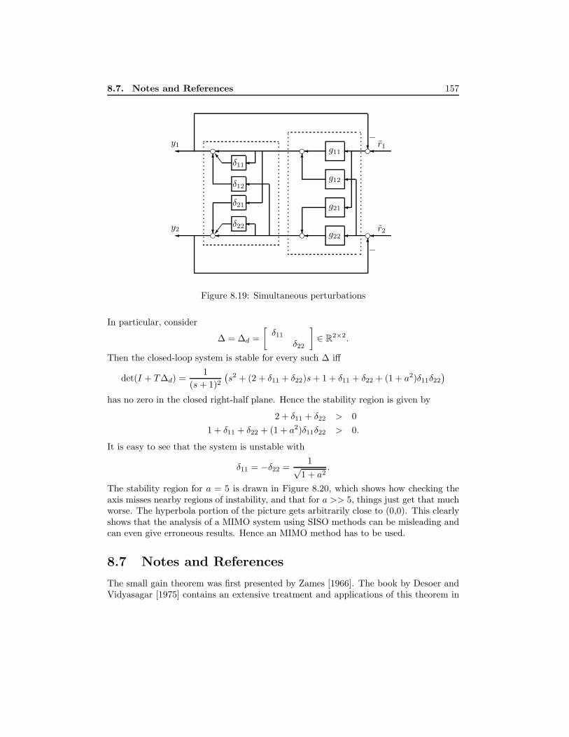
8.7. Notes and References 157
d
d
d
d d
d r2
r1
y2
y1 ?
6
?/
SSo6
δ21
δ12
δ22
δ11
?
6
g22
g21
g12
g11
−
−
Figure 8.19: Simultaneous perturbations
In particular, consider
∆ = ∆d =[δ11
δ22
]∈ R2×2.
Then the closed-loop system is stable for every such ∆ iff
det(I + T∆d) =1
(s+ 1)2
(s2 + (2 + δ11 + δ22)s+ 1 + δ11 + δ22 + (1 + a2)δ11δ22
)has no zero in the closed right-half plane. Hence the stability region is given by
2 + δ11 + δ22 > 01 + δ11 + δ22 + (1 + a2)δ11δ22 > 0.
It is easy to see that the system is unstable with
δ11 = −δ22 =1√
1 + a2.
The stability region for a = 5 is drawn in Figure 8.20, which shows how checking theaxis misses nearby regions of instability, and that for a >> 5, things just get that muchworse. The hyperbola portion of the picture gets arbitrarily close to (0,0). This clearlyshows that the analysis of a MIMO system using SISO methods can be misleading andcan even give erroneous results. Hence an MIMO method has to be used.
8.7 Notes and References
The small gain theorem was first presented by Zames [1966]. The book by Desoer andVidyasagar [1975] contains an extensive treatment and applications of this theorem in

158 UNCERTAINTY AND ROBUSTNESS
−2 −1.5 −1 −0.5 0 0.5 1 1.5
−2
−1.5
−1
−0.5
0
0.5
1
1.5
Figure 8.20: Stability region for a = 5
various forms. Robust stability conditions under various uncertainty assumptions arediscussed in Doyle, Wall, and Stein [1982].
8.8 Problems
Problem 8.1 This problem shows that the stability margin is critically dependent onthe type of perturbation. The setup is a unity-feedback loop with controller K(s) = 1and plant Pnom(s) + ∆(s), where
Pnom(s) =10
s2 + 0.2s+ 1.
1. Assume ∆(s) ∈ RH∞. Compute the largest β such that the feedback system isinternally stable for all ‖∆‖∞ < β.
2. Repeat but with ∆ ∈ R.
Problem 8.2 Let M ∈ Cp×q be a given complex matrix. Then it is shown in Qiu etal [1995] that I −∆M is invertible for all ∆ ∈ Rq×p such that σ(∆) ≤ γ if and only ifµ∆(M) < 1/γ, where
µ∆(M) = infα∈(0,1]
σ2
([ReM −α=Mα−1=M ReM
]).

8.8. Problems 159
It follows that (I−∆M(s))−1 ∈ RH∞ for a given M(s) ∈ RH∞ and all ∆ ∈ Rq×p withσ(∆) ≤ γ if and only if supω µ∆(M(jω)) < 1/γ. Write a Matlab program to computeµ∆(M) and apply it to the preceding problem.
Problem 8.3 Let G(s) =Ke−τs
Ts+ 1and K ∈ [10, 12], τ ∈ [0, 0.5], T = 1. Find a nominal
model Go(s) ∈ RH∞ and a weighting function W (s) ∈ RH∞ such that
G(s) ∈ Go(s) (1 +W (s)∆(s)) : ∆ ∈ H∞, ‖∆‖ ≤ 1 .
Problem 8.4 Think of an example of a physical system with the property that thenumber of unstable poles changes when the system undergoes a small change, for ex-ample, when a mass is perturbed slightly or the geometry is deformed slightly.
Problem 8.5 Let X be a space of scalar-valued transfer functions. A function f(s) inX is a unit if 1/f(s) is in X .
1. Prove that the set of units in RH∞ is an open set, that is, if f is a unit, then
(∃ε > 0) (∀g ∈ RH∞) ‖g‖∞ < ε =⇒ f + g is a unit. (8.11)
2. Here is an application of the preceding fact. Consider the unity feedback systemwith controller k(s) and plant p(s), both SISO, with k(s) proper and p(s) strictlyproper. Do coprime factorizations over RH∞:
p =npmp
, k =nkmk
.
Then the feedback system is internally stable iff npnk +mpmk is a unit in RH∞.Assume it is a unit. Perturb p(s) to
p =np + ∆n
mp + ∆m, ∆n,∆m ∈ RH∞.
Show that internal stability is preserved if ‖∆n‖∞ and ‖∆m‖∞ are small enough.The conclusion is that internal stability is preserved if the perturbations are smallenough in the H∞ norm.
3. Give an example of a unit f(s) in RH∞ such that equation (8.11) fails for the H2
norm, that is, such that
(∀ε > 0) (∃g ∈ RH2) ‖g‖2 < ε and f + g is not a unit.
What is the significance of this fact concerning robust stability?
Problem 8.6 Let ∆ and M be square constant matrices. Prove that the followingthree conditions are equivalent:

160 UNCERTAINTY AND ROBUSTNESS
1.[
I −∆−M I
]is invertible;
2. I −M∆ is invertible;
3. I −∆M is invertible.
Problem 8.7 Consider the unity feedback system
K Gj- - - -
6−
For
G(s) =
1s
1s
1s
1s
design a proper controller K(s) to stabilize the feedback system internally. Now perturbG(s) to
1 + ε
s
1s
1s
1s
, ε ∈ R.
Is the feedback system internally stable for all sufficiently small ε?
Problem 8.8 Consider the unity feedback system with K(s) = 3, G(s) =1
s− 2. Com-
pute by hand (i.e., without Matlab) a normalized coprime factorization of G(s). Con-sidering perturbations ∆N and ∆M of the factors of G(s), compute by hand the stabilityradius ε, that is, the least upper bound on
∥∥[ ∆N ∆M
]∥∥∞ such that feedback sta-
bility is preserved.
Problem 8.9 Let a unit feedback system with a controller K(s) =1s
and a nominal
plant model Po(s) =s+ 1
s2 + 0.2s+ 5. Construct a smallest destabilizing ∆ ∈ RH∞ in the
sense of ‖∆‖∞ for each of the following cases:
(a) P = Po + ∆;
(b) P = Po(1 +W∆) with W (s) =0.2(s+ 10)s+ 50
;

8.8. Problems 161
(c) P =N + ∆n
M + ∆m, N =
s+ 1(s+ 2)2
, M =s2 + 0.2s+ 5
(s+ 2)2, and ∆ =
[∆n ∆m
].
Problem 8.10 This problem concerns the unity feedback system with controller K(s)and plant
G(s) =1
s+ 1
[1 23 4
].
1. Take K(s) = kI2 (k a real scalar) and find the range of k for internal stability.
2. Take
K(s) =[k1 00 k2
](k1, k2 real scalars) and find the region of (k1, k2) in R2 for internal stability.
Problem 8.11 (Kharitonov’s Theorem) Let a(s) be an interval polynomial
a(s) = [a−0 , a+0 ] + [a−1 , a
+1 ]s+ [a−2 , a
+2 ]s2 + · · · .
Kharitonov’s theorem shows that a(s) is stable if and only if the following four Kharitonovpolynomials are stable:
K1(s) = a−0 + a−1 s+ a+2 s
2 + a+3 s
3 + a−4 s4 + a−5 s
5 + a+6 s
6 + · · ·
K2(s) = a−0 + a+1 s+ a+
2 s2 + a−3 s
3 + a−4 s4 + a+
5 s5 + a+
6 s6 + · · ·
K3(s) = a+0 + a+
1 s+ a−2 s2 + a−3 s
3 + a+4 s
4 + a+5 s
5 + a−6 s6 + · · ·
K4(s) = a+0 + a−1 s+ a−2 s
2 + a+3 s
3 + a+4 s
4 + a−5 s5 + a−6 s
6 + · · ·
Let ai := (a−i + a+i )/2 and let
anom(s) = a0 + a1s+ a2s2 + · · · .
Find a least conservative W (s) such that
a(s)anom(s)
∈ 1 +W (s)∆(s) | ‖∆‖∞ ≤ 1 .
Problem 8.12 One of the main tools in this chapter was the small-gain theorem. Oneway to state it is as follows: Define a transfer matrix F (s) in RH∞ to be contractiveif ‖F‖∞ ≤ 1 and strictly contractive if ‖F‖∞ < 1. Then for the unity feedback systemthe small gain theorem is this: If K is contractive and G is strictly contractive, thenthe feedback system is stable.
This problem concerns passivity and the passivity theorem. This is an importanttool in the study of the stability of feedback systems, especially robotics, that is com-plementary to the small gain theorem.

162 UNCERTAINTY AND ROBUSTNESS
Consider a system with a square transfer matrix F (s) in RH∞. This is said to bepassive if
F (jω) + F (jω)∗ ≥ 0, ∀ω.
Here, the symbol ≥ 0 means that the matrix is positive semidefinite. If the system isSISO, the condition is equivalent to
Re F (jω) ≥ 0, ∀ω;
that is, the Nyquist plot of F lies in the right-half plane. The system is strictly passiveif F − εI is passive for some ε > 0.
1. Consider a mechanical system with input vector u(t) (forces and torques) andoutput vector y(t) (velocities) modeled by the equation
My +Ky = u
where M and K are symmetric, positive definite matrices. Show that this systemis passive.
2. If F is passive, then (I + F )−1 ∈ RH∞ and (I + F )−1(I − F ) is contractive; ifF is strictly passive, then (I + F )−1(I − F ) is strictly contractive. Prove thesestatements for the case that F is SISO.
3. Using the results so far, show (in the MIMO case) that the unity feedback systemis stable if K is passive and G is strictly passive.
Problem 8.13 Consider a SISO feedback system shown below with P = Po +W2∆2.
e eK P
W3
- - -
?
? -6−
d
z
Assume that P0 and P have the same number of right-half plane poles, W2 is stable,and
|Re∆2| ≤ α, |=∆2| ≤ β.
Derive the necessary and sufficient conditions for the feedback system to be robustlystable.

8.8. Problems 163
Problem 8.14 Let P =[P11 P12
P21 P22
]∈ RH∞ be a two-by-two transfer matrix. Find
sufficient (and necessary, if possible) conditions in each case so that Fu(P,∆) is stablefor all possible stable ∆ that satisfies the following conditions, respectively:
1. at each frequencyRe∆(jω) ≥ 0, |∆(jω)| < α
2. at each frequencyRe∆(jω)e±jθ ≥ 0, |∆(jω)| < α
where θ ≥ 0.
3. at each frequency
Re∆(jω) ≥ 0,=∆(jω) ≥ 0,Re∆(jω) + =∆(jω) < α
Problem 8.15 Let P = (I + ∆W )P0 such that P and P0 have the same number ofunstable poles for all admissible ∆, ‖∆‖∞ < γ. Show that K robustly stabilizes P ifand only if K stabilizes P0 and∥∥WP0K(I + P0K)−1
∥∥∞ ≤ 1.
Problem 8.16 Give appropriate generalizations of the preceding problem to othertypes of uncertainties.
Problem 8.17 Let K = I and
P0 =
1
s+ 12
s+ 31
s+ 11
s+ 1
.1. Let P = P0 + ∆ with ‖∆‖∞ ≤ γ. Determine the largest γ for robust stability.
2. Let ∆ =[k1
k2
]∈ R2×2. Determine the stability region.
Problem 8.18 Repeat the preceding problem with
P0 =
s− 1
(s+ 1)2
5s+ 1(s+ 1)2
−1(s+ 1)2
s− 1(s+ 1)2
.

164 UNCERTAINTY AND ROBUSTNESS

Chapter 9
Linear FractionalTransformation
This chapter introduces a new matrix function: linear fractional transformation (LFT).We show that many interesting control problems can be formulated in an LFT frame-work and thus can be treated using the same technique.
9.1 Linear Fractional Transformations
This section introduces the matrix linear fractional transformations. It is well knownfrom the one-complex-variable function theory that a mapping F : C 7→ C of the form
F (s) =a+ bs
c+ ds
with a, b, c, and d ∈ C is called a linear fractional transformation. In particular, if c 6= 0then F (s) can also be written as
F (s) = α+ βs(1− γs)−1
for some α, β and γ ∈ C. The linear fractional transformation described above forscalars can be generalized to the matrix case.
Definition 9.1 Let M be a complex matrix partitioned as
M =[M11 M12
M21 M22
]∈ C(p1+p2)×(q1+q2),
and let ∆` ∈ Cq2×p2 and ∆u ∈ Cq1×p1 be two other complex matrices. Then we canformally define a lower LFT with respect to ∆` as the map
F`(M, •) : Cq2×p2 7→ Cp1×q1
165

166 LINEAR FRACTIONAL TRANSFORMATION
withF`(M,∆`) := M11 +M12∆`(I −M22∆`)−1M21
provided that the inverse (I −M22∆`)−1 exists. We can also define an upper LFT withrespect to ∆u as
Fu(M, •) : Cq1×p1 7→ Cp2×q2
withFu(M,∆u) = M22 +M21∆u(I −M11∆u)−1M12
provided that the inverse (I −M11∆u)−1 exists.
The matrix M in the preceding LFTs is called the coefficient matrix. The motivation forthe terminologies of lower and upper LFTs should be clear from the following diagramrepresentations of F`(M,∆`) and Fu(M,∆u):
y1 u1
w1z1
-
M
∆`
y2 u2
w2z2
-
M
∆u
The diagram on the left represents the following set of equations:[z1
y1
]= M
[w1
u1
]=[M11 M12
M21 M22
] [w1
u1
],
u1 = ∆` y1
while the diagram on the right represents[y2
z2
]= M
[u2
w2
]=[M11 M12
M21 M22
] [u2
w2
],
u2 = ∆u y2.
It is easy to verify that the mapping defined on the left diagram is equal to F`(M,∆`)and the mapping defined on the right diagram is equal to Fu(M,∆u). So from the abovediagrams, F`(M,∆`) is a transformation obtained from closing the lower loop on the leftdiagram; similarly, Fu(M,∆u) is a transformation obtained from closing the upper loopon the right diagram. In most cases, we shall use the general term LFT in referring toboth upper and lower LFTs and assume that the context will distinguish the situationssince one can use either of these notations to express a given object. Indeed, it is clear
that Fu(N,∆) = F`(M,∆) with N =[M22 M21
M12 M11
]. It is usually not crucial which
expression is used; however, it is often the case that one expression is more convenientthan the other for a given problem. It should also be clear to the reader that in writingF`(M,∆) [or Fu(M,∆)] it is implied that ∆ has compatible dimensions.

9.1. Linear Fractional Transformations 167
A useful interpretation of an LFT [e.g., F`(M,∆)] is that F`(M,∆) has a nominalmapping, M11, and is perturbed by ∆, while M12,M21, and M22 reflect a prior knowl-edge as to how the perturbation affects the nominal map, M11. A similar interpretationcan be applied to Fu(M,∆). This is why LFT is particularly useful in the study ofperturbations, which is the focus of the next chapter.
The physical meaning of an LFT in control science is obvious if we take M as a propertransfer matrix. In that case, the LFTs defined previously are simply the closed-looptransfer matrices from w1 7→ z1 and w2 7→ z2, respectively; that is,
Tzw1 = F`(M,∆`), Tzw2 = Fu(M,∆u)
where M may be the controlled plant and ∆ may be either the system model uncer-tainties or the controllers.
Definition 9.2 An LFT, F`(M,∆), is said to be well-defined (or well-posed) if(I −M22∆) is invertible.
Note that this definition is consistent with the well-posedness definition of the feed-back system, which requires that the corresponding transfer matrix be invertible inRp(s). It is clear that the study of an LFT that is not well-defined is meaningless;hence throughout this book, whenever an LFT is invoked, it will be assumed implicitlythat it is well-defined. It is also clear from the definition that, for any M , F`(M, 0)is well-defined; hence any function that is not well-defined at the origin cannot be ex-pressed as an LFT in terms of its variables. For example, f(δ) = 1/δ is not an LFT ofδ.
In some literature, LFT is used to refer to the following matrix functions:
(A+BQ)(C +DQ)−1 or (C +QD)−1(A+QB)
where C is usually assumed to be invertible due to practical consideration. The followingresults follow from some simple algebra.
Lemma 9.1 Suppose C is invertible. Then
(A+BQ)(C +DQ)−1 = F`(M,Q)(C +QD)−1(A+QB) = F`(N,Q)
with
M =[AC−1 B −AC−1DC−1 −C−1D
], N =
[C−1A C−1
B −DC−1A −DC−1
].
The converse also holds if M satisfies certain conditions.

168 LINEAR FRACTIONAL TRANSFORMATION
Lemma 9.2 Let F`(M,Q) be a given LFT with M =[M11 M12
M21 M22
].
(a) If M12 is invertible, then
F`(M,Q) = (C +QD)−1(A+QB)
with A = M−112 M11, B = M21 −M22M
−112 M11, C = M−1
12 , and D = −M22M−112 ;
that is,
[A CB D
]= F`
0 0 −IM21 0 M22
M11 I 0
,−M−112
= F`
0 0 −IM21 0 M22
M11 I M12 +E
, E−1
for any nonsingular matrix E.
(b) If M21 is invertible, then
F`(M,Q) = (A+BQ)(C +DQ)−1
with A = M11M−121 , B = M12 −M11M
−121 M22, C = M−1
21 , and D = −M−121 M22;
that is,
[A BC D
]= F`
0 M12 M11
0 0 I−I M22 0
,−M−121
= F`
0 M12 M11
0 0 I−I M22 M21 +E
, E−1
for any nonsingular matrix E.
However, for an arbitrary LFT F`(M,Q), neither M21 nor M12 is necessarily squareand invertible; therefore, the alternative fractional formula is more restrictive.
It should be pointed out that some seemingly simple functions do not have simpleLFT representations. For example,
(A+QB)(I +QD)−1
cannot always be written in the form of F`(M,Q) for some M ; however, it can bewritten as
(A+QB)(I +QD)−1 = F`(N,∆)

9.1. Linear Fractional Transformations 169
with
N =
A I A−B 0 −BD 0 D
, ∆ =[Q
Q
].
Note that the dimension of ∆ is twice of Q.The following lemma shows that the inverse of an LFT is still an LFT.
Lemma 9.3 Let M =[M11 M12
M21 M22
]and M22 is nonsingular. Then
(Fu(M,∆))−1 = Fu(N,∆)
with N , is given by
N =[M11 −M12M
−122 M21 −M12M
−122
M−122 M21 M−1
22
].
LFT is a very convenient tool to formulate many mathematical objects. We shallillustrate this by the following two examples.
Simple Block Diagrams
A feedback system with the following block diagram
F
K
W1
P W2i i
i- - - - -
?
?
6
y
uf
u
d
v
n
−
can be rearranged as an LFT:
G
K
z
y
w
u
-
with
w =(dn
), z =
(vuf
), G =
W2P 0 W2P0 0 W1
−FP −F −FP
.

170 LINEAR FRACTIONAL TRANSFORMATION
A state-space realization for the generalized plant G can be obtained by directlyrealizing the transfer matrix G using any standard multivariable realization techniques(e.g., Gilbert realization). However, the direct realization approach is usually com-plicated. Here we shall show another way to obtain the realization for G based onthe realizations of each component. To simplify the expression, we shall assume thatthe plant P is strictly proper and P , F , W1, and W2 have, respectively, the followingstate-space realizations:
P =[Ap BpCp 0
], F =
[Af BfCf Df
], W1 =
[Au BuCu Du
], W2 =
[Av BvCv Dv
].
That is,xp = Apxp +Bp(d+ u), yp = Cpxp,
xf = Afxf +Bf (yp + n), −y = Cfxf +Df(yp + n),
xu = Auxu +Buu, uf = Cuxu +Duu,
xv = Avxv +Bvyp, v = Cvxv +Dvyp.
Now define a new state vector
x =
xpxfxuxv
and eliminate the variable yp to get a realization of G as
x = Ax+B1w +B2u
z = C1x+D11w +D12u
y = C2x+D21w +D22u
with
A =
Ap 0 0 0BfCp Af 0 0
0 0 Au 0BvCp 0 0 Av
, B1 =
Bp 00 Bf0 00 0
, B2 =
Bp0Bu0
C1 =
[DvCp 0 0 Cv
0 0 Cu 0
], D11 = 0, D12 =
[0Du
]C2 =
[−DfCp −Cf 0 0
], D21 =
[0 −Df
], D22 = 0.

9.1. Linear Fractional Transformations 171
Parametric Uncertainty: A Mass/Spring/Damper System
One natural type of uncertainty is unknown coefficients in a state-space model. Tomotivate this type of uncertainty description, we shall begin with a familiar mechanicalsystem, shown in Figure 9.1.
m
6F
XXXX
XXX ck
Figure 9.1: A mass/spring/damper system
The dynamical equation of the system motion can be described by
x+c
mx+
k
mx =
F
m.
Suppose that the three physical parameters m, c, and k are not known exactly, but arebelieved to lie in known intervals. In particular, the actual mass m is within 10% ofa nominal mass, m, the actual damping value c is within 20% of a nominal value ofc, and the spring stiffness is within 30% of its nominal value of k. Now introducingperturbations δm, δc, and δk, which are assumed to be unknown but lie in the interval[−1, 1], the block diagram for the dynamical system is as shown in Figure 9.2.
It is easy to check that 1m can be represented as an LFT in δm:
1m
=1
m(1 + 0.1δm)=
1m− 0.1
mδm(1 + 0.1δm)−1 = F` (M1, δm)
with M1 =
[1m − 0.1
m
1 −0.1
]. Suppose that the input signals of the dynamical system
are selected as x1 = x, x2 = x, F , and the output signals are selected as x1 and x2. Torepresent the system model as an LFT of the natural uncertainty parameters δm, δc, andδk, we shall first isolate the uncertainty parameters and denote the inputs and outputsof δk, δc, and δm as yk, yc, ym and uk, uc, um, respectively, as shown in Figure 9.3.

172 LINEAR FRACTIONAL TRANSFORMATION
k(1 + 0.3δk)
c(1 + 0.2δc)
1m(1+0.1δm)
1s
1s
−d
d+
-
- -6
6
Fxxx
Figure 9.2: Block diagram of mass/spring/damper equation
e
ee
e
M1
1s
1s
δm-
c
0.2 δc
6
- --
- -6
k
0.3 δk
6-
--
6
-
−
x2x1
ym um
ucyc
yk uk
F
Figure 9.3: A block diagram for the mass/spring/damper system with uncertain pa-rameters

9.2. Basic Principle 173
Then
x1
x2
yk
yc
ym
=
0 1 0 0 0 0− km − c
m1m − 1
m − 1m − 0.1
m
0.3k 0 0 0 0 00 0.2c 0 0 0 0−k −c 1 −1 −1 −0.1
x1
x2
F
uk
uc
um
,
uk
uc
um
= ∆
yk
yc
ym
.
That is, [x1
x2
]= F`(M,∆)
x1
x2
F
where
M =
0 1 0 0 0 0− km − c
m1m − 1
m − 1m − 0.1
m
0.3k 0 0 0 0 00 0.2c 0 0 0 0−k −c 1 −1 −1 −0.1
, ∆ =
δk 0 00 δc 00 0 δm
.
9.2 Basic Principle
We have studied two simple examples of the use of LFTs and, in particular, their role inmodeling uncertainty. The basic principle at work here in writing a matrix LFT is oftenreferred to as “pulling out the ∆’s”. We will try to illustrate this with another picture.Consider a structure with four substructures interconnected in some known way, asshown in Figure 9.4. This diagram can be redrawn as a standard one via “pulling outthe ∆’s” in Figure 9.5.
Now the matrix M of the LFT can be obtained by computing the correspondingtransfer matrix in the shadowed box.
We shall illustrate the preceding principle with an example. Consider an input/outputrelation
z =a+ bδ2 + cδ1δ
22
1 + dδ1δ2 + eδ21
w =: Gw
where a, b, c, d, and e are given constants or transfer functions. We would like to writeG as an LFT in terms of δ1 and δ2. We shall do this in three steps:
1. Draw a block diagram for the input/output relation with each δ separated asshown in Figure 9.6.

174 LINEAR FRACTIONAL TRANSFORMATION
....
.
....
.
....
.
......
..
....
....
......
..
......
.....
.....
....
.
....
.
.....
.....
...
....
......
.
.....
. ......
......
......
....
......
.
......
......
......
......
..
......
......
......
.....
......
......
......
.. ............
......
......
......
......
.
......
......
.
......
.....
......
.
...... . . . . .
.. .. .. .. .............
...........
.....................
.....................
.....................
.......................
..........................
..............................
........
........
........
........
......
..... ......
..... ...........
........
......
......
..
.........
.......
.......
....
......
.........
....
∆3
∆2
∆1
K
Figure 9.4: Multiple source of uncertain structure
....
.
....
.
....
.
......
..
....
....
......
..
......
.....
.....
....
.
....
.
.....
.....
...
....
......
.
.....
. ......
......
......
....
......
.
......
......
......
......
..
......
......
......
.....
......
......
......
.. ............
......
......
......
......
.
......
......
.
......
.....
......
.
...... . . . . .
.. .. .. .. .............
...........
.....................
.....................
.....................
.......................
..........................
..............................
........
........
........
........
......
..... ......
..... ...........
........
......
......
..
.........
.......
.......
....
......
.........
....
-
-
-
?
-
K
∆3
∆2
∆1
Figure 9.5: Pulling out the ∆’s
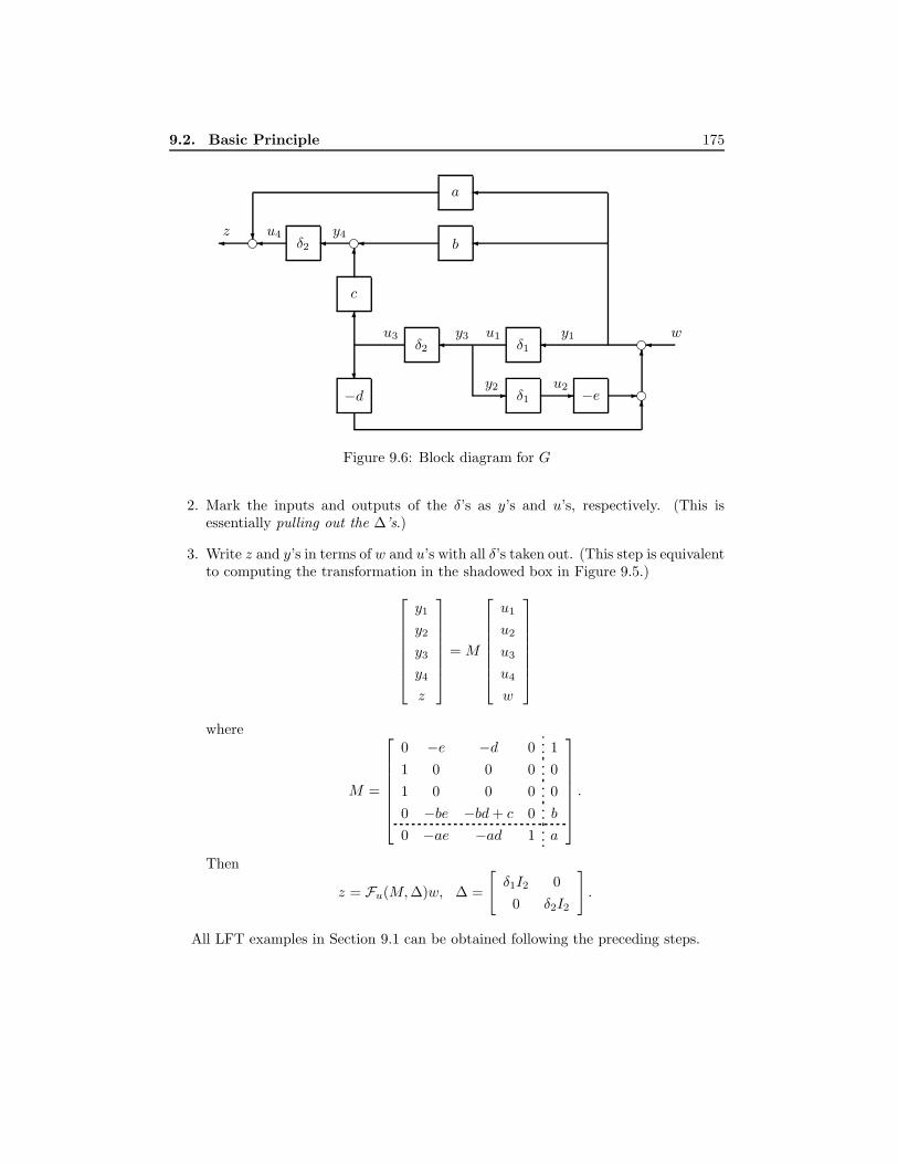
9.2. Basic Principle 175
e e
ee
δ2 δ1
δ1 −e−d
c
b
a
δ2
-
6
-
6
?
6-
6
?
z u4 y4
u3 y3 u1 y1
y2 u2
w
Figure 9.6: Block diagram for G
2. Mark the inputs and outputs of the δ’s as y’s and u’s, respectively. (This isessentially pulling out the ∆’s.)
3. Write z and y’s in terms of w and u’s with all δ’s taken out. (This step is equivalentto computing the transformation in the shadowed box in Figure 9.5.)
y1
y2
y3
y4
z
= M
u1
u2
u3
u4
w
where
M =
0 −e −d 0 11 0 0 0 01 0 0 0 00 −be −bd+ c 0 b
0 −ae −ad 1 a
.
Then
z = Fu(M,∆)w, ∆ =
[δ1I2 0
0 δ2I2
].
All LFT examples in Section 9.1 can be obtained following the preceding steps.

176 LINEAR FRACTIONAL TRANSFORMATION
For Simulink users, it is much easier to do all the computations using Simulink
block diagrams, as shown in the following example.
Example 9.1 Consider the HIMAT (highly maneuverable aircraft) control problemfrom the µ Analysis and Synthesis Toolbox (Balas et al. [1994]). The system diagramis shown in Figure 9.7 where
Wdel =
50(s+ 100)s+ 10000
0
050(s+ 100)s+ 10000
, Wp =
0.5(s+ 3)s+ 0.03
0
00.5(s+ 3)s+ 0.03
,
Wn =
2(s+ 1.28)s+ 320
0
02(s+ 1.28)s+ 320
,
P0 =
−0.0226 −36.6 −18.9 −32.1 0 00 −1.9 0.983 0 −0.414 0
0.0123 −11.7 −2.63 0 −77.8 22.40 0 1 0 0 0
0 57.3 0 0 0 00 0 0 57.3 0 0
f f
fP0 Wp
WnK
Wdel
-6
∆-
?- - ? - -
?
[d1
d2
]
[n1
n2
]
[e1
e2
]
[z1
z2
][p1
p2
]
u y
Figure 9.7: HIMAT closed-loop interconnection

9.2. Basic Principle 177
The open-loop interconnection is
z1
z2
e1
e2
y1
y2
= G(s)
p1
p2
d1
d2
n1
n2
u1
u2
.
The Simulink block diagram of this open-loop interconnection is shown in Figure 9.8.
Figure 9.8: Simulink block diagram for HIMAT (aircraft.m)
The G(s) =
[A B
C D
]can be computed by
[A,B,C,D] = linmod(′aircraft′)

178 LINEAR FRACTIONAL TRANSFORMATION
which gives
A =
−10000I2 0 0 0 0 0 0 0
0 −0.0226 −36.6 −18.9 −32.1 0 0 0
0 0 −1.9 0.983 0 0 0 0
0 0.0123 −11.7 −2.63 0 0 0 0
0 0 0 1 0 0 0 0
0 0 −54.087 0 0 −0.018 0 0
0 0 0 0 −54.087 0 −0.018 0
0 0 0 0 0 0 0 −320I2
B =
0 0 0 0 −703.5624 0
0 0 0 0 0 −703.5624
0 0 0 0 0 0
−0.4140 0 0 0 −0.4140 0
−77.8 22.4 0 0 −77.8 22.4
0 0 0 0 0 0
0 0 −0.9439I2 0 0 0
0 0 0 −25.2476I2 0 0
C =
703.5624I2 0 0 0 0 0 0 0 0
0 0 28.65 0 0 −0.9439 0 0 0
0 0 0 0 28.65 0 −0.9439 0 0
0 0 57.3 0 0 0 0 25.2476 0
0 0 0 0 57.3 0 0 0 25.2476
D =
0 0 0 0 0 0 50 0
0 0 0 0 0 0 0 50
0 0 0.5 0 0 0 0 0
0 0 0 0.5 0 0 0 0
0 0 1 0 2 0 0 0
0 0 0 1 0 2 0 0
.
9.3 Redheffer Star Products
The most important property of LFTs is that any interconnection of LFTs is again anLFT. This property is by far the most often used and is the heart of LFT machinery.Indeed, it is not hard to see that most of the interconnection structures discussed earlier(e.g., feedback and cascade) can be viewed as special cases of the so-called star product.

9.3. Redheffer Star Products 179
Suppose that P and K are compatibly partitioned matrices
P =
[P11 P12
P21 P22
], K =
[K11 K12
K21 K22
]such that the matrix product P22K11 is well-defined and square, and assume furtherthat I − P22K11 is invertible. Then the star product of P and K with respect to thispartition is defined as
P ? K :=
[Fl (P,K11) P12 (I −K11P22)−1
K12
K21 (I − P22K11)−1P21 Fu (K,P22)
]. (9.1)
Note that this definition is dependent on the partitioning of the matrices P and K. Infact, this star product may be well-defined for one partition and not well-defined foranother; however, we will not explicitly show this dependence because it is always clearfrom the context. In a block diagram, this dependence appears, as shown in Figure 9.9.
z w
wzw
wz
z
y u
!!!!
!!aaaaaa
P ? K
K
P
Figure 9.9: Interconnection of LFTs
Now suppose that P and K are transfer matrices with state-space representations:
P =
A B1 B2
C1 D11 D12
C2 D21 D22
K =
AK BK1 BK2
CK1 DK11 DK12
CK2 DK21 DK22
.Then the transfer matrix
P ? K :
[w
w
]7→[z
z
]has a representation
P ? K =
A B1 B2
C1 D11 D12
C2 D21 D22
=
[A B
C D
]

180 LINEAR FRACTIONAL TRANSFORMATION
where
A =
[A+B2R
−1DK11C2 B2R−1CK1
BK1R−1C2 AK +BK1R
−1D22CK1
]
B =
[B1 +B2R
−1DK11D21 B2R−1DK12
BK1R−1D21 BK2 +BK1R
−1D22DK12
]
C =
[C1 +D12DK11R
−1C2 D12R−1CK1
DK21R−1C2 CK2 +DK21R
−1D22CK1
]
D =
[D11 +D12DK11R
−1D21 D12R−1DK12
DK21R−1D21 DK22 +DK21R
−1D22DK12
]
R = I −D22DK11, R = I −DK11D22.
In fact, it is easy to show that
A =
[A B2
C2 D22
]?
[DK11 CK1
BK1 AK
],
B =
[B1 B2
D21 D22
]?
[DK11 DK12
BK1 BK2
],
C =
[C1 D12
C2 D22
]?
[DK11 CK1
DK21 CK2
],
D =
[D11 D12
D21 D22
]?
[DK11 DK12
DK21 DK22
].
The Matlab command starp can be used to compute the star product:
P ?K = starp(P,K,dimy,dimu)
where dimy and dimu are the dimensions of y and u, respectively. In the particular casewhen dim(z) = 0 and dim(w) = 0, we have
F`(P,K) = starp(P,K)
9.4 Notes and References
This chapter is based on the lecture notes by Packard [1991] and the paper by Doyle,Packard, and Zhou [1991].

9.5. Problems 181
9.5 Problems
Problem 9.1 Find M and N matrices such that ∆ = M∆N , where ∆ is block diago-nal.
1. ∆ =[
∆1 ∆2
]2. ∆ =
(∆1 0 00 0 ∆2
)
3. ∆ =
∆1
[0 0
][
∆2
0
]∆3
4. ∆ =
∆1 0 0∆2 ∆3 00 0 ∆4
5. ∆ =
∆1 ∆3 0∆2 ∆4 ∆6
0 ∆5 0
Problem 9.2 Let G = (I − P (s)∆)−1. Find a matrix M(s) such that G = Fu(M,∆).
Problem 9.3 Consider the unity feedback system with G(s) of size 2 × 2. SupposeG(s) has an uncertainty model of the form
G(s) =
[[1 + ∆11(s)]g11(s) [1 + ∆12(s)]g12(s)[1 + ∆21(s)]g21(s) [1 + ∆22(s)]g22(s)
].
Suppose also that we wish to study robust stability of the feedback system. Pull out the∆’s and draw the appropriate block diagram in the form of a structured perturbationof a nominal system.
Problem 9.4 Let
P (s) =
A B1 B2
C1 D11 D12
C2 D21 D22
, K(s) =
[A B
C D
].
Find state-space realizations for F`(P,K) and F`(P, D).

182 LINEAR FRACTIONAL TRANSFORMATION
Problem 9.5 Suppose D21 is nonsingular and
M(s) =
A B1 B2
C1 D11 D12
C2 D21 D22
.Find a state-space realization for
M(s) =
[
0 M12
0 0
] [M11
I
][−I M22
]M21 +E
where E is a constant matrix. Find the state-space realization for F`(M,E−1) whenE = I.

Chapter 10
µ and µ Synthesis
It is noted that the robust stability and robust performance criteria derived in Chap-ter 8 vary with the assumptions about the uncertainty descriptions and performancerequirements. We shall show in this chapter that they can all be treated in a unifiedframework using the LFT machinery introduced in the last chapter and the structuredsingular value to be introduced in this chapter. This, of course, does not mean thatthose special problems and their corresponding results are not important; on the con-trary, they are sometimes very enlightening to our understanding of complex problems,such as those in which complex problems are formed from simple problems. On theother hand, a unified approach may relieve the mathematical burden of dealing withspecific problems repeatedly. Furthermore, the unified framework introduced here willenable us to treat exactly the robust stability and robust performance problems forsystems with multiple sources of uncertainties, which is a formidable problem from thestandpoint of Chapter 8, in the same fashion as single unstructured uncertainty. In-deed, if a system is subject to multiple sources of uncertainties, in order to use theresults in Chapter 8 for unstructured cases, it is necessary to reflect all sources of un-certainties from their known point of occurrence to a single reference location in theloop. Such reflected uncertainties invariably have a great deal of structure, which mustthen be “covered up” with a large, arbitrarily more conservative perturbation in orderto maintain a simple cone-bounded representation at the reference location. Readersmight have some idea about the conservativeness in such reflection based on the skewedspecification problem, where an input multiplicative uncertainty of the plant is reflectedat the output and the size of the reflected uncertainty is proportional to the conditionnumber of the plant. In general, the reflected uncertainty may be proportional to thecondition number of the transfer matrix between its original location and the reflectedlocation. Thus it is highly desirable to treat the uncertainties as they are and wherethey are. The structured singular value is defined exactly for that purpose.
183
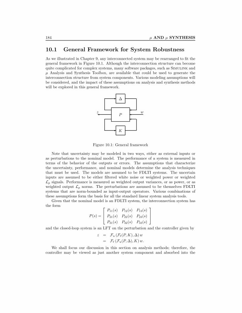
184 µ AND µ SYNTHESIS
10.1 General Framework for System Robustness
As we illustrated in Chapter 9, any interconnected system may be rearranged to fit thegeneral framework in Figure 10.1. Although the interconnection structure can becomequite complicated for complex systems, many software packages, such as Simulink andµ Analysis and Synthesis Toolbox, are available that could be used to generate theinterconnection structure from system components. Various modeling assumptions willbe considered, and the impact of these assumptions on analysis and synthesis methodswill be explored in this general framework.
wz
-
-
K
∆
P
Figure 10.1: General framework
Note that uncertainty may be modeled in two ways, either as external inputs oras perturbations to the nominal model. The performance of a system is measured interms of the behavior of the outputs or errors. The assumptions that characterizethe uncertainty, performance, and nominal models determine the analysis techniquesthat must be used. The models are assumed to be FDLTI systems. The uncertaininputs are assumed to be either filtered white noise or weighted power or weightedLp signals. Performance is measured as weighted output variances, or as power, or asweighted output Lp norms. The perturbations are assumed to be themselves FDLTIsystems that are norm-bounded as input-output operators. Various combinations ofthese assumptions form the basis for all the standard linear system analysis tools.
Given that the nominal model is an FDLTI system, the interconnection system hasthe form
P (s) =
P11(s) P12(s) P13(s)P21(s) P22(s) P23(s)P31(s) P32(s) P33(s)
and the closed-loop system is an LFT on the perturbation and the controller given by
z = Fu (F`(P,K),∆)w= F` (Fu(P,∆),K)w.
We shall focus our discussion in this section on analysis methods; therefore, thecontroller may be viewed as just another system component and absorbed into the

10.1. General Framework for System Robustness 185
interconnection structure. Denote
M(s) = F` (P (s),K(s)) =
[M11(s) M12(s)M21(s) M22(s)
].
Then the general framework reduces to Figure 10.2, where
z = Fu(M,∆)w =[M22 +M21∆(I −M11∆)−1M12
]w.
wz
-
M
∆
Figure 10.2: Analysis framework
SupposeK(s) is a stabilizing controller for the nominal plant P . ThenM(s) ∈ RH∞.In general, the stability of Fu(M,∆) does not necessarily imply the internal stability ofthe closed-loop feedback system. However, they can be made equivalent with suitablychosen w and z. For example, consider again the multiplicatively perturbed systemshown in Figure 10.3.
e e e- K P
W2 ∆ W1
- - - -
- - -
?
6
?d1 e1
d2
e2
e3 d3
−
Figure 10.3: Multiplicatively perturbed systems
Now let
w :=
[d1
d2
], z :=
[e1
e2
].
Then the system is robustly stable for all ∆(s) ∈ RH∞ with ‖∆‖∞ < 1 if and only ifFu(M,∆) ∈ RH∞ for all admissible ∆ with M11 = −W2PK(I + PK)−1W1, which isguaranteed by ‖M11‖∞ ≤ 1.
The analysis results presented in the previous chapters together with the associ-ated synthesis tools are summarized in Table 10.1 with various uncertainty modelingassumptions.
However, the analysis is not so simple for systems with multiple sources of modeluncertainties, including the robust performance problem for systems with unstructured

186 µ AND µ SYNTHESIS
Input Performance Perturbation Analysis SynthesisAssumptions Specifications Assumptions Tests Methods
E(w(t)w(τ)∗) E(z(t)∗z(t)) ≤ 1 LQG= δ(t− τ)I
∆ = 0 ‖M22‖2 ≤ 1 Wiener-Hopfw = U0δ(t) E(‖z‖22) ≤ 1
E(U0U∗0 ) = I H2
‖w‖2 ≤ 1 ‖z‖2 ≤ 1 ∆ = 0 ‖M22‖∞ ≤ 1 Singular ValueLoop Shaping
‖w‖2 ≤ 1 Internal Stability ‖∆‖∞ < 1 ‖M11‖∞ ≤ 1 H∞
Table 10.1: General analysis for single source of uncertainty
uncertainty. As we shown in Chapter 9, if a system is built from components that arethemselves uncertain, then, in general, the uncertainty in the system level is structured,involving typically a large number of real parameters. The stability analysis involvingreal parameters is much more difficult and will be discussed in Chapter 18. Here we shallsimply cover the real parametric uncertainty with norm-bounded dynamical uncertainty.Moreover, the interconnection model M can always be chosen so that ∆(s) is blockdiagonal, and, by absorbing any weights, ‖∆‖∞ < 1. Thus we shall assume that ∆(s)takes the form of
∆(s) = diag [δ1Ir1 , . . . , δsIrS ,∆1, . . . ,∆F ] : δi(s) ∈ RH∞, ∆j ∈ RH∞
with ‖δi‖∞ < 1 and ‖∆j‖∞ < 1. Then the system is robustly stable iff the intercon-nected system in Figure 10.4 is stable.
The results of Table 10.1 can be applied to analysis of the system’s robust stabilityin two ways:
(1) ‖M11‖∞ ≤ 1 implies stability, but not conversely, because this test ignores theknown block diagonal structure of the uncertainties and is equivalent to regarding∆ as unstructured. This can be arbitrarily conservative in that stable systems canhave arbitrarily large ‖M11‖∞.

10.2. Structured Singular Value 187
......
-
-
...
M11(s)
∆F (s)
δ1(s)I
Figure 10.4: Robust stability analysis framework
(2) Test for each δi (∆j) individually (assuming no uncertainty in other channels).This test can be arbitrarily optimistic because it ignores interaction between theδi (∆j). This optimism is also clearly shown in the spinning body example inSection 8.6.
The difference between the stability margins (or bounds on ∆) obtained in (1) and (2)can be arbitrarily far apart. Only when the margins are close can conclusions be madeabout the general case with structured uncertainty.
The exact stability and performance analysis for systems with structured uncertaintyrequires a new matrix function called the structured singular value (SSV), which isdenoted by µ.
10.2 Structured Singular Value
10.2.1 Definitions of µ
We shall motivate the definition of the structured singular value by asking the followingquestion: Given a matrixM ∈ Cp×q, what is the smallest perturbation matrix ∆ ∈ Cq×pin the sense of σ(∆) such that
det(I −M∆) = 0?
That is, we are interested in finding
αmin := infσ(∆) : det(I −M∆) = 0, ∆ ∈ Cq×p
.

188 µ AND µ SYNTHESIS
It is easy to see that
αmin = infα : det(I − αM∆) = 0, σ(∆) ≤ 1, ∆ ∈ Cq×p
=
1maxσ(∆)≤1
ρ(M∆)
andmaxσ(∆)≤1
ρ(M∆) = σ(M).
Hence the smallest norm of a “destabilizing” perturbation matrix is 1/σ(M) with asmallest “destabilizing” ∆:
∆des =1
σ(M)v1u∗1, det(I −M∆des) = 0
where M = σ(M)u1v∗1 + σ2u2v
∗2 + · · · is a singular value decomposition.
So the reciprocal of the largest singular value of a matrix is a measure of the smallest“destabilizing” perturbation matrix. Hence it is instructive to introduce the followingalternative definition for the largest singular value:
σ(M) :=1
infσ(∆) : det(I −M∆) = 0, ∆ ∈ Cq×p .
Next we consider a similar problem but with ∆ structurally restricted. In particular,we consider the block diagonal matrix ∆. We shall consider two types of blocks: repeatedscalar and full blocks. Let S and F represent the number of repeated scalar blocks andthe number of full blocks, respectively. To bookkeep their dimensions, we introducepositive integers r1, . . . , rS ; m1, . . . ,mF . The ith repeated scalar block is ri × ri, whilethe jth full block is mj ×mj . With those integers given, we define ∆ ⊂ Cn×n as
∆ =
diag [δ1Ir1 , . . . , δsIrS ,∆1, . . . ,∆F ] : δi ∈ C,∆j ∈ Cmj×mj. (10.1)
For consistency among all the dimensions, we must have
S∑i=1
ri +F∑j=1
mj = n.
Often, we will need norm-bounded subsets of ∆, and we introduce the following nota-tion:
B∆ = ∆ ∈∆ : σ(∆) ≤ 1 (10.2)
Bo∆ = ∆ ∈∆ : σ(∆) < 1 (10.3)
where the superscript “o” symbolizes the open ball. To keep the notation as simple aspossible in equation (10.1), we place all of the repeated scalar blocks first; in actuality,they can come in any order. Also, the full blocks do not have to be square, but restrictingthem as such saves a great deal in terms of notation.

10.2. Structured Singular Value 189
Now we ask a similar question: Given a matrix M ∈ Cp×q, what is the smallestperturbation matrix ∆ ∈∆ in the sense of σ(∆) such that
det(I −M∆) = 0?
That is, we are interested in finding
αmin := inf σ(∆) : det(I −M∆) = 0, ∆ ∈∆ .
Again we have
αmin = inf α : det(I − αM∆) = 0, ∆ ∈ B∆ =1
max∆∈B∆
ρ(M∆).
Similar to the unstructured case, we shall call 1/αmin the structured singular value anddenote it by µ∆(M).
Definition 10.1 For M ∈ Cn×n,µ∆(M) is defined as
µ∆(M) :=1
min σ(∆) : ∆ ∈∆,det (I −M∆) = 0 (10.4)
unless no ∆ ∈∆ makes I −M∆ singular, in which case µ∆(M) := 0.
Remark 10.1 Without a loss in generality, the full blocks in the minimal norm ∆ caneach be chosen to be dyads (rank = 1). To see this, assume S = 0 (i.e., all blocks arefull blocks). Suppose that I−M∆ is singular for some ∆ ∈∆. Then there is an x ∈ Cnsuch that M∆x = x. Now partition x conformably with ∆:
x =
x1
x2
...xF
, xi ∈ Cmi , i = 1, . . . , F
and let
∆i =
∆ixix
∗i
‖xi‖2, xi 6= 0;
0, xi = 0
for i = 1, 2, . . . , F.
Define∆ = diag∆1, ∆2, . . . , ∆F .
Then σ(∆) ≤ σ(∆), ∆x = ∆x, and thus (I −M∆)x = (I −M∆)x = 0 (i.e., I −M∆is also singular). Hence we have replaced a general perturbation ∆ that satisfies thesingularity condition with a perturbation ∆ that is no larger [in the σ(·) sense] and hasrank 1 for each block but still satisfies the singularity condition. 3

190 µ AND µ SYNTHESIS
Lemma 10.1 µ∆(M) = max∆∈B∆
ρ (M∆)
In view of this lemma, continuity of the function µ :Cn×n→R is apparent. In general,though, the function µ :Cn×n→R is not a norm, since it does not satisfy the triangleinequality; however, for any α ∈ C, µ (αM) = |α|µ (M), so in some sense, it is relatedto how “big” the matrix is.
We can relate µ∆(M) to familiar linear algebra quantities when ∆ is one of twoextreme sets.
• If ∆ = δI : δ ∈ C (S = 1, F = 0, r1 = n), then µ∆(M) = ρ (M), the spectralradius of M .
Proof. The only ∆’s in ∆ that satisfy the det (I −M∆) = 0 constraint arereciprocals of nonzero eigenvalues of M . The smallest one of these is associatedwith the largest (magnitude) eigenvalue, so, µ∆(M) = ρ (M). 2
• If ∆ = Cn×n (S=0, F =1,m1 =n), then µ∆(M) = σ(M).
Obviously, for a general ∆, as in equation (10.1), we must have
δIn : δ ∈ C ⊂∆ ⊂ Cn×n. (10.5)
Hence directly from the definition of µ and from the two preceding special cases, weconclude that
ρ (M) ≤ µ∆(M) ≤ σ (M) . (10.6)
These bounds alone are not sufficient for our purposes because the gap between ρ andσ can be arbitrarily large.
Example 10.1 Suppose
∆ =
[δ1 00 δ2
]and consider
(1) M =
[0 β
0 0
]for any β > 0. Then ρ(M) = 0 and σ(M) = β. But µ(M) = 0
since det(I −M∆) = 1 for all admissible ∆.
(2) M =
[−1/2 1/2−1/2 1/2
]. Then ρ(M) = 0 and σ(M) = 1. Since
det(I −M∆) = 1 +δ1 − δ2
2,
it is easy to see that min
maxi |δi| : 1 + δ1−δ22 = 0
= 1, so µ(M) = 1.

10.2. Structured Singular Value 191
Thus neither ρ nor σ provide useful bounds even in simple cases. The only time theydo provide reliable bounds is when ρ ≈ σ.
However, the bounds can be refined by considering transformations on M that donot affect µ∆(M), but do affect ρ and σ. To do this, define the following two subsetsof Cn×n:
U = U ∈∆ : UU∗ = In (10.7)
D =
diag
[D1, . . . , DS , d1Im1 , . . . , dF−1ImF−1 , ImF
]:
Di ∈ Cri×ri , Di = D∗i > 0, dj ∈ R, dj > 0
. (10.8)
Note that for any ∆ ∈∆, U ∈ U , and D ∈ D,
U∗ ∈ U U∆ ∈∆ ∆U ∈∆ σ (U∆) = σ (∆U) = σ (∆) (10.9)
D∆ = ∆D. (10.10)
Consequently, we have the following:
Theorem 10.2 For all U ∈ U and D ∈ D
µ∆(MU) = µ∆(UM) = µ∆(M) = µ∆
(DMD−1
). (10.11)
Proof. For all D ∈ D and ∆ ∈∆,
det (I −M∆) = det(I −MD−1∆D
)= det
(I −DMD−1∆
)since D commutes with ∆. Therefore µ∆(M) = µ∆
(DMD−1
). Also, for each
U ∈ U , det (I −M∆) = 0 if and only if det (I −MUU∗∆) = 0. Since U∗∆ ∈ ∆and σ (U∗∆) = σ (∆), we get µ∆ (MU) = µ∆(M) as desired. The argument for UM isthe same. 2
Therefore, the bounds in equation (10.6) can be tightened to
maxU∈U
ρ(UM) ≤ max∆∈B∆
ρ (∆M) = µ∆(M) ≤ infD∈D
σ(DMD−1
)(10.12)
where the equality comes from Lemma 10.1. Note that the last element in the D matrixis normalized to 1 since for any nonzero scalar γ, DMD−1 = (γD)M (γD)−1.
Remark 10.2 Note that the scaling set D in Theorem 10.2 and in inequality (10.12)is not necessarily restricted to being Hermitian. In fact, it can be replaced by any set ofnonsingular matrices that satisfy equation (10.10). However, enlarging the set of scalingmatrices does not improve the upper-bound in inequality (10.12). This can be shown

192 µ AND µ SYNTHESIS
as follows: Let D be any nonsingular matrix such that D∆ = ∆D. Then there exist aHermitian matrix 0 < R = R∗ ∈ D and a unitary matrix U such that D = UR and
infDσ(DMD−1
)= inf
Dσ(URMR−1U∗
)= infR∈D
σ(RMR−1
).
Therefore, there is no loss of generality in assuming D to be Hermitian. 3
10.2.2 Bounds
In this section we will concentrate on the bounds
maxU∈U
ρ (UM) ≤ µ∆(M) ≤ infD∈D
σ(DMD−1
).
The lower bound is always an equality (Doyle [1982]).
Theorem 10.3 maxU∈U
ρ(MU) = µ∆(M)
Unfortunately, the quantity ρ (UM) can have multiple local maxima that are not global.Thus local search cannot be guaranteed to obtain µ, but can only yield a lower bound.For computation purposes one can derive a slightly different formulation of the lowerbound as a power algorithm that is reminiscent of power algorithms for eigenvalues andsingular values (Packard and Doyle [1988a, 1988b]). While there are open questionsabout convergence, the algorithm usually works quite well and has proven to be aneffective method to compute µ.
The upper-bound can be reformulated as a convex optimization problem, so theglobal minimum can, in principle, be found. Unfortunately, the upper-bound is notalways equal to µ. For block structures ∆ satisfying 2S + F ≤ 3, the upper-bound isalways equal to µ∆(M), and for block structures with 2S+F > 3, there exist matricesfor which µ is less than the infimum. This can be summarized in the following diagram,which shows for which cases the upper-bound is guaranteed to be equal to µ. SeePackard and Doyle [1993] for details.
Theorem 10.4 µ∆(M) = infD∈D
σ(DMD−1) if 2S + F ≤ 3
F= 0 1 2 3 4S=
0 yes yes yes no
1 yes yes no no no
2 no no no no no
Several of the boxes have connections with standard results.
• S = 0, F = 1 : µ∆(M) = σ (M).

10.2. Structured Singular Value 193
• S = 1, F = 0 : µ∆(M) = ρ (M) = infD∈D
σ(DMD−1
). This is a standard result in
linear algebra. In fact, without a loss in generality, the matrix M can be assumedin Jordan canonical form. Now let
J1 =
λ 1λ 1
. . . . . .
λ 1λ
, D1 =
1k
. . .
kn1−2
kn1−1
∈ Cn1×n1 .
Then infD1∈Cn1×n1
σ(D1J1D−11 ) = lim
k→∞σ(D1J1D
−11 ) = |λ|. (Note that by Re-
mark 10.2, the scaling matrix does not need to be Hermitian.) The conclusionfollows by applying this result to each Jordan block.
That µ equals to the preceding upper-bound in this case is also equivalent to thefact that Lyapunov asymptotic stability and exponential stability are equivalentfor discrete time systems. This is because ρ (M) < 1 (exponential stability of adiscrete time system matrix M) implies for some nonsingular D ∈ Cn×n
σ(DMD−1) < 1 or (D−1)∗M∗D∗DMD−1 − I < 0,
which, in turn, is equivalent to the existence of a P = D∗D > 0 such that
M∗PM − P < 0
(Lyapunov asymptotic stability).
• S = 0, F = 2 : This case was studied by Redheffer [1959].
• S = 1, F = 1 : This is equivalent to a state-space characterization of the H∞norm of a discrete time transfer function.
• S = 2, F = 0 : This is equivalent to the fact that for multidimensional systems(two dimensional, in fact), exponential stability is not equivalent to Lyapunovstability.
• S = 0, F ≥ 4 : For this case, the upper-bound is not always equal to µ. Thisis important, as these are the cases that arise most frequently in applications.Fortunately, the bound seems to be close to µ. The worst known example has aratio of µ over the bound of about .85, and most systems are close to 1.
The preceding bounds are much more than just computational schemes. They arealso theoretically rich and can unify a number of apparently different results in linearsystems theory. There are several connections with Lyapunov asymptotic stability,two of which were hinted at previously, but there are further connections between the

194 µ AND µ SYNTHESIS
upper-bound scalings and solutions to Lyapunov and Riccati equations. Indeed, manymajor theorems in linear systems theory follow from the upper-bounds and from someresults of linear fractional transformations. The lower bound can be viewed as a naturalgeneralization of the maximum modulus theorem.
Of course, one of the most important uses of the upper-bound is as a computationalscheme when combined with the lower bound. For reliable use of the µ theory, it isessential to have upper and lower bounds. Another important feature of the upper-bound is that it can be combined with H∞ controller synthesis methods to yield an adhoc µ-synthesis method. Note that the upper-bound when applied to transfer functionsis simply a scaled H∞ norm. This is exploited in the D − K iteration procedure toperform approximate µ synthesis (Doyle [1982]), which will be briefly introduced inSection 10.4.
The upper and lower bounds of the structured singular value and the scaling matrixD can be computed using the MATLAB command
[bounds,rowd] = mu(M,blk)
where the structure of the ∆ is specified by a two-column matrix blk. for example, a
∆ =
δ1I2 0 0 0 0 00 δ2 0 0 0 00 0 ∆3 0 0 00 0 0 ∆4 0 00 0 0 0 δ5I3 00 0 0 0 0 ∆6
δ1, δ2, δ5,∈ C, ∆3 ∈ C2×3,∆4 ∈ C3×3,∆6 ∈ C2×1
can be specified by
blk =
2 01 12 33 33 02 1
.
Note that ∆j is not required to be square. The outputs of the program include a 2× 1vector bounds containing the upper and lower bounds of µ∆(M) and the row vectorrowd containing the scaling D. The D matrix can be recovered by
[D`,Dr] = unwrapd(rowd,blk)
where D` and Dr denote the left and right scaling matrices used in computing theupper-bound inf σ
(D`MD−1
r
)when some full blocks are not necessarily square and
they are equal if all full blocks are square.

10.2. Structured Singular Value 195
Example 10.2 Let
M =
j 2 2j 0 −1 −1 + 3j 2 + 3j3 + j 2− j −1 + j 2 + j −1 + j 1 −1 + j
3 + j j 2 + 2j −1 + 2j 3− j 3j −1 + j
−1 + j −1− j j 0 1− j 2− j 2 + 2j3 j 1 + j 3j 1 + j 3j −j1 3 + 2j 2 + 2j 3j 1 + 2j 2 + j −1 + 2j
2 + j −1− j −1 3 + 3j 2 + 3j 2j 1− j
and
∆ =
∆ =
δ1I2
δ2
∆3
∆4
: δ1, δ2 ∈ C,∆3 ∈ C2×3,∆4 ∈ C2×1
.
Then blk =
2 01 12 32 1
and the Matlab program gives bounds =[
10.5955 10.5518]
and
D` =
D1
0.76380.8809I3
1.0293
Dr =
D1
0.76380.8809I2
1.0293I2
where
D1 =
[1.0260− 0.0657j 0.2174− 0.3471j−0.0701 + 0.3871j −0.4487− 0.6953j
].
In fact, D` and Dr can be replaced by Hermitian matrices without changing the upper-bound by replacing D1 with
D1 =
[1.0992 0.0041− 0.0591j
0.0041 + 0.0591j 0.9215
]

196 µ AND µ SYNTHESIS
since D1 = U1D1 and
U1 =
[0.9155− 0.0713j 0.2365− 0.3177j−0.1029 + 0.3824j −0.5111− 0.7629j
]is a unitary matrix.
10.2.3 Well-Posedness and Performance for Constant LFTs
Let M be a complex matrix partitioned as
M =
[M11 M12
M21 M22
](10.13)
and suppose there are two defined block structures, ∆1 and ∆2, which are compatiblein size with M11 and M22, respectively. Define a third structure ∆ as
∆ =
[∆1 00 ∆2
]: ∆1 ∈∆1,∆2 ∈∆2
. (10.14)
Now we may compute µ with respect to three structures. The notations we use to keeptrack of these computations are as follows: µ1 (·) is with respect to ∆1, µ2 (·) is withrespect to ∆2, and µ∆(·) is with respect to ∆. In view of these notations, µ1 (M11),µ2 (M22), and µ∆(M) all make sense, though, for instance, µ1 (M) does not.
This section is interested in following constant matrix problems:
• Determine whether the LFT F` (M,∆2) is well-defined for all ∆2 ∈ ∆2 withσ(∆2) ≤ β (< β).
• If so, determine how “large” F` (M,∆2) can get for this norm-bounded set ofperturbations.
Let ∆2 ∈∆2. Recall that F` (M,∆2) is well-defined if I −M22∆2 is invertible. Thefirst theorem is nothing more than a restatement of the definition of µ.
Theorem 10.5 The linear fractional transformation F` (M,∆2) is well-defined
(a) for all ∆2 ∈ B∆2 if and only if µ2 (M22) < 1.
(b) for all ∆2 ∈ Bo∆2 if and only if µ2 (M22) ≤ 1.
As the “perturbation” ∆2 deviates from zero, the matrix F` (M,∆2) deviates fromM11. The range of values that µ1 (F` (M,∆2)) takes on is intimately related to µ∆(M),as shown in the following theorem:
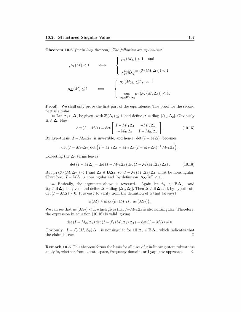
10.2. Structured Singular Value 197
Theorem 10.6 (main loop theorem) The following are equivalent:
µ∆(M) < 1 ⇐⇒
µ2 (M22) < 1, and
max∆2∈B∆2
µ1 (F` (M,∆2)) < 1
µ∆(M) ≤ 1 ⇐⇒
µ2 (M22) ≤ 1, and
sup∆2∈Bo∆2
µ1 (F` (M,∆2)) ≤ 1.
Proof. We shall only prove the first part of the equivalence. The proof for the secondpart is similar.⇐ Let ∆i ∈∆i be given, with σ (∆i) ≤ 1, and define ∆ = diag [∆1,∆2]. Obviously
∆ ∈∆. Now
det (I −M∆) = det
[I −M11∆1 −M12∆2
−M21∆1 I −M22∆2
]. (10.15)
By hypothesis I −M22∆2 is invertible, and hence det (I −M∆) becomes
det (I −M22∆2) det(I −M11∆1 −M12∆2 (I −M22∆2)−1
M21∆1
).
Collecting the ∆1 terms leaves
det (I −M∆) = det (I −M22∆2) det (I −F` (M,∆2) ∆1) . (10.16)
But µ1 (F` (M,∆2)) < 1 and ∆1 ∈ B∆1, so I −F` (M,∆2) ∆1 must be nonsingular.Therefore, I −M∆ is nonsingular and, by definition, µ∆(M) < 1.
⇒ Basically, the argument above is reversed. Again let ∆1 ∈ B∆1 and∆2 ∈ B∆2 be given, and define ∆ = diag [∆1,∆2]. Then ∆ ∈ B∆ and, by hypothesis,det (I −M∆) 6= 0. It is easy to verify from the definition of µ that (always)
µ (M) ≥ max µ1 (M11) , µ2 (M22) .
We can see that µ2 (M22) < 1, which gives that I−M22∆2 is also nonsingular. Therefore,the expression in equation (10.16) is valid, giving
det (I −M22∆2) det (I −F` (M,∆2) ∆1) = det (I −M∆) 6= 0.
Obviously, I − F` (M,∆2) ∆1 is nonsingular for all ∆i ∈ B∆i, which indicates thatthe claim is true. 2
Remark 10.3 This theorem forms the basis for all uses of µ in linear system robustnessanalysis, whether from a state-space, frequency domain, or Lyapunov approach. 3

198 µ AND µ SYNTHESIS
The role of the block structure ∆2 in the main loop theorem is clear — it is thestructure that the perturbations come from; however, the role of the perturbation struc-ture ∆1 is often misunderstood. Note that µ1 (·) appears on the right-hand side ofthe theorem, so that the set ∆1 defines what particular property of F` (M,∆2) isconsidered. As an example, consider the theorem applied with the two simple blockstructures considered right after Lemma 10.1. Define ∆1 := δ1In : δ1 ∈ C. Hence,for A ∈ Cn×n, µ1 (A) = ρ (A). Likewise, define ∆2 = Cm×m; then for D ∈ Cm×m,µ2 (D) = σ(D). Now, let ∆ be the diagonal augmentation of these two sets, namely
∆ :=
[δ1In 0n×m0m×n ∆2
]: δ1 ∈ C,∆2 ∈ Cm×m
⊂ C(n+m)×(n+m).
Let A ∈ Cn×n, B ∈ Cn×m, C ∈ Cm×n, and D ∈ Cm×m be given, and interpret them asthe state-space model of a discrete time system
xk+1 = Axk +Buk
yk = Cxk +Duk.
Let M ∈ C(n+m)×(n+m) be the block state-space matrix of the system
M =
[A B
C D
].
Applying the theorem with these data gives that the following are equivalent:
• The spectral radius of A satisfies ρ (A) < 1, and
maxδ1∈C|δ1|≤1
σ(D + Cδ1 (I −Aδ1)−1B
)< 1. (10.17)
• The maximum singular value of D satisfies σ(D) < 1, and
max∆2∈Cm×mσ(∆2)≤1
ρ(A+B∆2 (I −D∆2)−1
C)< 1. (10.18)
• The structured singular value of M satisfies
µ∆(M) < 1. (10.19)
The first condition is recognized by two things: The system is stable, and the || · ||∞norm on the transfer function from u to y is less than 1 (by replacing δ1 with 1
z ):
‖G‖∞ := maxz∈C|z|≥1
σ(D + C (zI −A)−1B
)= max
δ1∈C|δ1|≤1
σ(D + Cδ1 (I −Aδ1)−1B
).

10.2. Structured Singular Value 199
The second condition implies that (I −D∆2)−1 is well defined for all σ(∆2) ≤ 1 andthat a robust stability result holds for the uncertain difference equation
xk+1 =(A+B∆2 (I −D∆2)−1C
)xk
where ∆2 is any element in Cm×m with σ(∆2) ≤ 1, but otherwise unknown.This equivalence between the small gain condition, ‖G‖∞ < 1, and the stability
robustness of the uncertain difference equation is well-known. This is the small gaintheorem, in its necessary and sufficient form for linear, time invariant systems with oneof the components norm bounded, but otherwise unknown. What is important to noteis that both of these conditions are equivalent to a condition involving the structuredsingular value of the state-space matrix. Already we have seen that special cases of µ arethe spectral radius and the maximum singular value. Here we see that other importantlinear system properties — namely, robust stability and input-output gain — are alsorelated to a particular case of the structured singular value.
Example 10.3 Let M , ∆1, and ∆2 be defined as in the beginning of this section. Nowsuppose µ2(M22) < 1. Find
max∆2∈B∆2
µ1 (F` (M,∆2)) .
This can be done iteratively as follows:
max∆2∈B∆2
µ1 (F` (M,∆2)) = α
⇐⇒ max∆2∈B∆2
µ1
(F`
([M11/α M12/α
M21 M22
],∆2
))= 1
⇐⇒ µ∆
([M11/α M12/α
M21 M22
])= 1.
Hence
max∆2∈B∆2
µ1 (F` (M,∆2)) =
α : µ∆
([M11/α M12/α
M21 M22
])= 1
.
For example, let ∆1 = δI2, ∆2 ∈ C2×2:
A =
[0.1 0.21 0
], B =
[1 01 1
], C =
[1 21 3
], D =
[0.5 00 0.8
].
Findαmax = sup
σ(∆2)≤1
ρ(A+B∆2(I −D∆2)−1C).
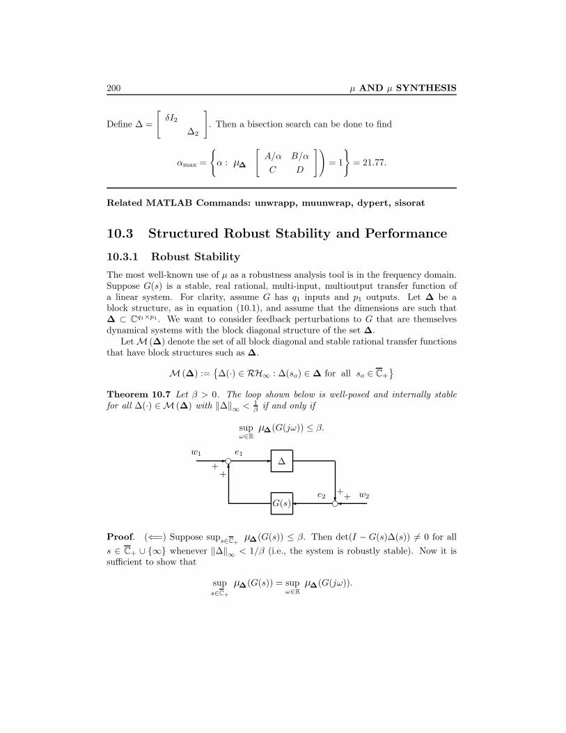
200 µ AND µ SYNTHESIS
Define ∆ =
[δI2
∆2
]. Then a bisection search can be done to find
αmax =
α : µ∆
([A/α B/α
C D
])= 1
= 21.77.
Related MATLAB Commands: unwrapp, muunwrap, dypert, sisorat
10.3 Structured Robust Stability and Performance
10.3.1 Robust Stability
The most well-known use of µ as a robustness analysis tool is in the frequency domain.Suppose G(s) is a stable, real rational, multi-input, multioutput transfer function ofa linear system. For clarity, assume G has q1 inputs and p1 outputs. Let ∆ be ablock structure, as in equation (10.1), and assume that the dimensions are such that∆ ⊂ Cq1×p1 . We want to consider feedback perturbations to G that are themselvesdynamical systems with the block diagonal structure of the set ∆.
LetM (∆) denote the set of all block diagonal and stable rational transfer functionsthat have block structures such as ∆.
M (∆) :=
∆(·) ∈ RH∞ : ∆(so) ∈∆ for all so ∈ C+
Theorem 10.7 Let β > 0. The loop shown below is well-posed and internally stablefor all ∆(·) ∈ M (∆) with ‖∆‖∞ < 1
β if and only if
supω∈R
µ∆(G(jω)) ≤ β.
ee
++
++e2
e1
w2
w1
-6
?
-
G(s)
∆
Proof. (⇐=) Suppose sups∈C+µ∆(G(s)) ≤ β. Then det(I − G(s)∆(s)) 6= 0 for all
s ∈ C+ ∪ ∞ whenever ‖∆‖∞ < 1/β (i.e., the system is robustly stable). Now it issufficient to show that
sups∈C+
µ∆(G(s)) = supω∈R
µ∆(G(jω)).

10.3. Structured Robust Stability and Performance 201
It is clear that
sups∈C+
µ∆(G(s)) = sups∈C+
µ∆(G(s)) ≥ supωµ∆(G(jω)).
Now suppose sups∈C+µ∆(G(s)) > β; then by the definition of µ, there is an so ∈
C+∪∞ and a complex structured ∆ such that σ(∆) < 1/β and det(I−G(so)∆) = 0.This implies that there is a 0 ≤ ω ≤ ∞ and 0 < α ≤ 1 such that det(I −G(jω)α∆) =0. This, in turn, implies that µ∆(G(jω)) > β since σ(α∆) < 1/β. In other words,sups∈C+
µ∆(G(s)) ≤ supω µ∆(G(jω)). The proof is complete.(=⇒) Suppose supω∈R µ∆(G(jω)) > β. Then there is a 0 < ωo < ∞ such that
µ∆(G(jωo)) > β. By Remark 10.1, there is a complex ∆c ∈ ∆ that each full blockhas rank 1 and σ(∆c) < 1/β such that I −G(jωo)∆c is singular. Next, using the sameconstruction used in the proof of the small gain theorem (Theorem 8.1), one can find arational ∆(s) such that ‖∆(s)‖∞ = σ(∆c) < 1/β, ∆(jωo) = ∆c, and ∆(s) destabilizesthe system. 2
Hence, the peak value on the µ plot of the frequency response determines the sizeof perturbations that the loop is robustly stable against.
Remark 10.4 The internal stability with a closed ball of uncertainties is more compli-cated. The following example is shown in Tits and Fan [1995]. Consider
G(s) =1
s+ 1
[0 −11 0
]and ∆ = δ(s)I2. Then
supω∈R
µ∆(G(jω)) = supω∈R
1|jω + 1| = µ∆(G(j0)) = 1.
On the other hand, µ∆(G(s)) < 1 for all s 6= 0, s ∈ C+, and the only matrices in theform of Γ = γI2 with |γ| ≤ 1 for which
det(I −G(0)Γ) = 0
are the complex matrices ±jI2. Thus, clearly, (I − G(s)∆(s))−1 ∈ RH∞ for all realrational ∆(s) = δ(s)I2 with ‖δ‖∞ ≤ 1 since ∆(0) must be real. This shows thatsupω∈R µ∆(G(jω)) < 1 is not necessary for (I −G(s)∆(s))−1 ∈ RH∞ with the closedball of structured uncertainty ‖∆‖∞ ≤ 1. Similar examples with no repeated blocks aregenerated by setting G(s) = 1
s+1M , where M is any real matrix with µ∆(M) = 1 forwhich there is no real ∆ ∈∆ with σ(∆) = 1 such that det(I −M∆) = 0. For example,let
M =
0 β
γ α
γ −α
[ −β α α
0 −γ γ
], ∆ =
δ1
δ2
δ3
, δi ∈ C

202 µ AND µ SYNTHESIS
with γ2 = 12 and β2 + 2α2 = 1. Then it is shown in Packard and Doyle [1993] that
µ∆(M) = 1 and all ∆ ∈ ∆ with σ(∆) = 1 that satisfy det(I −M∆) = 0 must becomplex. 3
Remark 10.5 Let ∆ ∈ RH∞ be a structured uncertainty and
G(s) =
[G11(s) G12(s)G21(s) G22(s)
]∈ RH∞.
Then Fu(G,∆) ∈ RH∞ does not necessarily imply (I − G11∆)−1 ∈ RH∞ whether ∆is in an open ball or is in a closed ball. For example, consider
G(s) =
1s+1 0 10 10
s+1 01 0 0
and ∆ =
[δ1
δ2
]with ‖∆‖∞ < 1. Then Fu(G,∆) =
11− δ1 1
s+1
∈ RH∞ for all
admissible ∆ (‖∆‖∞ < 1) but (I −G11∆)−1 ∈ RH∞ is true only for ‖∆‖∞ < 0.1. 3
10.3.2 Robust Performance
Often, stability is not the only property of a closed-loop system that must be robust toperturbations. Typically, there are exogenous disturbances acting on the system (windgusts, sensor noise) that result in tracking and regulation errors. Under perturbation,the effect that these disturbances have on error signals can greatly increase. In mostcases, long before the onset of instability, the closed-loop performance will degrade tothe point of unacceptability (hence the need for a “robust performance” test). Sucha test will indicate the worst-case level of performance degradation associated with agiven level of perturbations.
Assume Gp is a stable, real-rational, proper transfer function with q1 + q2 inputsand p1 + p2 outputs. Partition Gp in the obvious manner
Gp(s) =
[G11 G12
G21 G22
]so that G11 has q1 inputs and p1 outputs, and so on. Let ∆ ⊂ Cq1×p1 be a blockstructure, as in equation (10.1). Define an augmented block structure:
∆P :=
[∆ 00 ∆f
]: ∆ ∈∆,∆f ∈ Cq2×p2
.
The setup is to address theoretically the robust performance questions about thefollowing loop:

10.3. Structured Robust Stability and Performance 203
wz
-
Gp(s)
∆(s)
The transfer function from w to z is denoted by Fu (Gp,∆).
Theorem 10.8 Let β > 0. For all ∆(s) ∈ M (∆) with ‖∆‖∞ < 1β , the loop shown
above is well-posed, internally stable, and ‖Fu (Gp,∆)‖∞ ≤ β if and only if
supω∈R
µ∆P(Gp(jω)) ≤ β.
Note that by internal stability, supω∈R µ∆(G11(jω)) ≤ β, then the proof of thistheorem is exactly along the lines of the earlier proof for Theorem 10.7, but also appealsto Theorem 10.6. This is a remarkably useful theorem. It says that a robust performanceproblem is equivalent to a robust stability problem with augmented uncertainty ∆, asshown in Figure 10.5.
-
-
∆f
∆
Gp(s)
Figure 10.5: Robust performance vs robust stability
Example 10.4 We shall consider again the HIMAT problem from Example 9.1. Usethe Simulink block diagram in Example 9.1 and run the following commands to getan interconnection model G, an H∞ stabilizing controller K and a closed-loop transfermatrix Gp(s) = F`(G,K). (Do not bother to figure out how hinfsyn works; it will beconsidered in detail in Chapter 14.)

204 µ AND µ SYNTHESIS
[A,B,C,D] = linmod(′aircraft′)
G = pck(A,B,C,D);
[K,Gp, γ] = hinfsyn(G,2,2,0,10,0.001,2);
which gives γ = 1.8612 = ‖Gp‖∞, a stabilizing controller K, and a closed loop transfermatrix Gp:
z1
z2
e1
e2
= Gp(s)
p1
p2
d1
d2
n1
n2
, Gp(s) =
[Gp11 Gp12
Gp21 Gp22
].
10−3
10−2
10−1
100
101
102
103
0
0.5
1
1.5
2
frequency (rad/sec)
maximum singular value
Figure 10.6: Singular values of Gp(jω)
Now generate the singular value frequency responses of Gp:
w=logspace(-3,3,300);
Gpf = frsp(Gp,w); % Gpf is the frequency response of Gp;
[u, s,v] = vsvd(Gpf);

10.3. Structured Robust Stability and Performance 205
vplot(′liv,m′, s)
The singular value frequency responses of Gp are shown in Figure 10.6. To test therobust stability, we need to compute ‖Gp11‖∞:
Gp11 = sel(Gp,1 : 2,1 : 2);
norm of Gp11 = hinfnorm(Gp11,0.001);
which gives ‖GP11‖∞ = 0.933 < 1. So the system is robustly stable. To check therobust performance, we shall compute the µ∆P (Gp(jω)) for each frequency with
∆P =
[∆
∆f
], ∆ ∈ C2×2, ∆f ∈ C4×2.
10−3
10−2
10−1
100
101
102
103
0.5
1
1.5
2
frequency (rad/sec)
Maximum Singular Value and mu
maximum singular value
mu bounds
Figure 10.7: µ∆P (Gp(jω)) and σ(Gp(jω))
blk=[2,2;4,2];
[bnds,dvec,sens,pvec]=mu(Gpf,blk);
vplot(′liv,m′,vnorm(Gpf),bnds)
title(′Maximum Singular Value and mu′)
xlabel(′frequency(rad/sec)′)
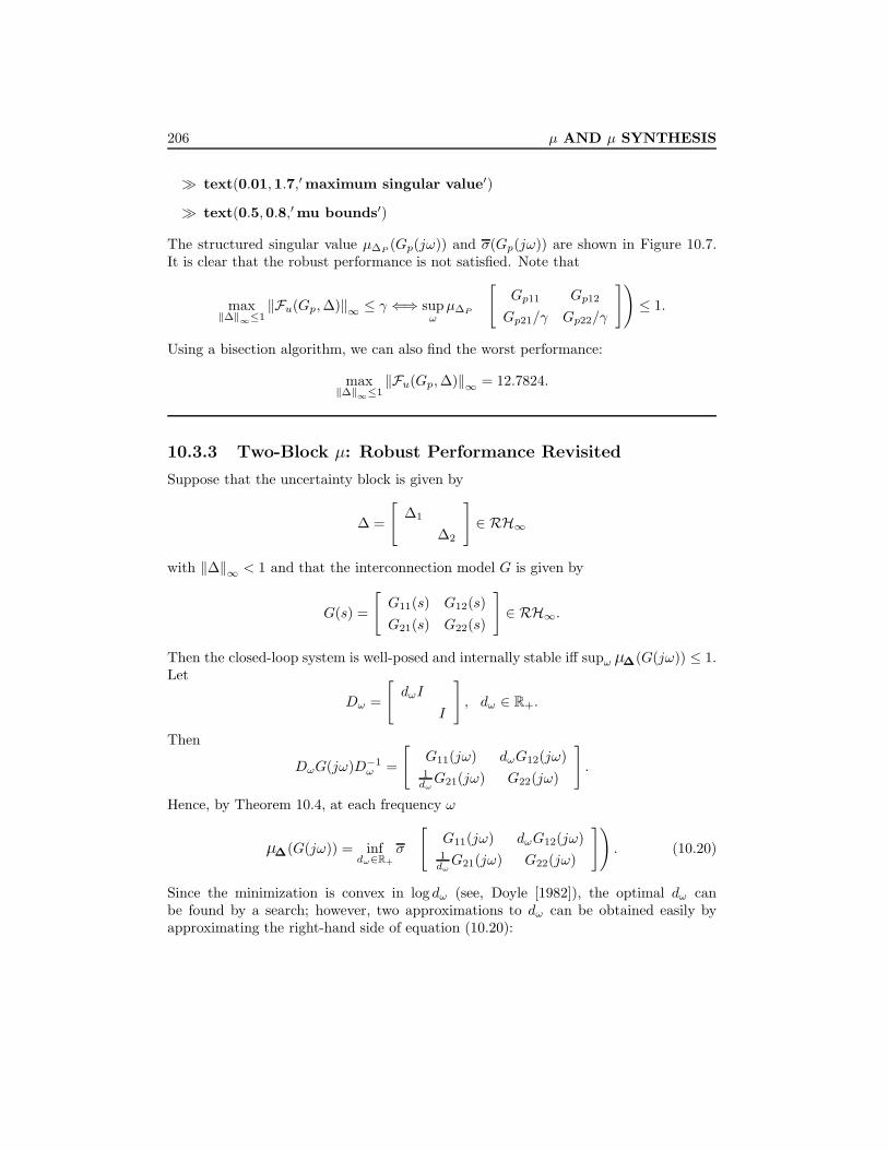
206 µ AND µ SYNTHESIS
text(0.01,1.7,′maximum singular value′)
text(0.5,0.8,′mu bounds′)
The structured singular value µ∆P (Gp(jω)) and σ(Gp(jω)) are shown in Figure 10.7.It is clear that the robust performance is not satisfied. Note that
max‖∆‖∞≤1
‖Fu(Gp,∆)‖∞ ≤ γ ⇐⇒ supωµ∆P
([Gp11 Gp12
Gp21/γ Gp22/γ
])≤ 1.
Using a bisection algorithm, we can also find the worst performance:
max‖∆‖∞≤1
‖Fu(Gp,∆)‖∞ = 12.7824.
10.3.3 Two-Block µ: Robust Performance Revisited
Suppose that the uncertainty block is given by
∆ =
[∆1
∆2
]∈ RH∞
with ‖∆‖∞ < 1 and that the interconnection model G is given by
G(s) =
[G11(s) G12(s)G21(s) G22(s)
]∈ RH∞.
Then the closed-loop system is well-posed and internally stable iff supω µ∆(G(jω)) ≤ 1.Let
Dω =
[dωI
I
], dω ∈ R+.
Then
DωG(jω)D−1ω =
[G11(jω) dωG12(jω)1dωG21(jω) G22(jω)
].
Hence, by Theorem 10.4, at each frequency ω
µ∆(G(jω)) = infdω∈R+
σ
([G11(jω) dωG12(jω)1dωG21(jω) G22(jω)
]). (10.20)
Since the minimization is convex in log dω (see, Doyle [1982]), the optimal dω canbe found by a search; however, two approximations to dω can be obtained easily byapproximating the right-hand side of equation (10.20):

10.3. Structured Robust Stability and Performance 207
(1) Note that
µ∆(G(jω)) ≤ infdω∈R+
σ
([‖G11(jω)‖ dω ‖G12(jω)‖
1dω‖G21(jω)‖ ‖G22(jω)‖
])
≤√
infdω∈R+
(‖G11(jω)‖2 + d2
ω ‖G12(jω)‖2 +1d2ω
‖G21(jω)‖2 + ‖G22(jω)‖2)
=√‖G11(jω)‖2 + ‖G22(jω)‖2 + 2 ‖G12(jω)‖ ‖G21(jω)‖
with the minimizing dω given by
dω =
√‖G21(jω)‖‖G12(jω)‖ if G12 6= 0 & G21 6= 0,
0 if G21 = 0,∞ if G12 = 0.
(10.21)
(2) Alternative approximation can be obtained by using the Frobenius norm:
µ∆(G(jω)) ≤ infdω∈R+
∥∥∥∥∥[
G11(jω) dωG12(jω)1dωG21(jω) G22(jω)
]∥∥∥∥∥F
=
√inf
dω∈R+
(‖G11(jω)‖2F + d2
ω ‖G12(jω)‖2F +1d2ω
‖G21(jω)‖2F + ‖G22(jω)‖2F)
=√‖G11(jω)‖2F + ‖G22(jω)‖2F + 2 ‖G12(jω)‖F ‖G21(jω)‖F
with the minimizing dω given by
dω =
√‖G21(jω)‖F‖G12(jω)‖F
if G12 6= 0 & G21 6= 0,
0 if G21 = 0,∞ if G12 = 0.
(10.22)
It can be shown that the approximations for the scalar dω obtained previously are exactfor a 2 × 2 matrix G. For higher dimensional G, the approximations for dω are stillreasonably good. Hence an approximation of µ can be obtained as
µ∆(G(jω)) ≤ σ([
G11(jω) dωG12(jω)1
dωG21(jω) G22(jω)
])(10.23)

208 µ AND µ SYNTHESIS
or, alternatively, as
µ∆(G(jω)) ≤ σ([
G11(jω) dωG12(jω)1dωG21(jω) G22(jω)
]). (10.24)
We can now see how these approximated µ tests are compared with the sufficientconditions obtained in Chapter 8.
Example 10.5 Consider again the robust performance problem of a system with out-put multiplicative uncertainty in Chapter 8 (see Figure 8.10):
P∆ = (I +W1∆W2)P, ‖∆‖∞ < 1.
Then it is easy to show that the problem can be put in the general framework byselecting
G(s) =
[−W2ToW1 −W2ToWd
WeSoW1 WeSoWd
]and that the robust performance condition is satisfied if and only if
‖W2ToW1‖∞ ≤ 1 (10.25)
and‖Fu(G,∆)‖∞ ≤ 1 (10.26)
for all ∆ ∈ RH∞ with ‖∆‖∞ < 1. But equations (10.25) and (10.26) are satisfied ifffor each frequency ω
µ∆(G(jω)) = infdω∈R+
σ
([−W2ToW1 −dωW2ToWd
1dωWeSoW1 WeSoWd
])≤ 1.
Note that, in contrast to the sufficient condition obtained in Chapter 8, this condition isan exact test for robust performance. To compare the µ test with the criteria obtainedin Chapter 8, some upper-bounds for µ can be derived. Let
dω =
√‖WeSoW1‖‖W2ToWd‖
.
Then, using the first approximation for µ, we get
µ∆(G(jω)) ≤√‖W2ToW1‖2 + ‖WeSoWd‖2 + 2 ‖W2ToWd‖ ‖WeSoW1‖
≤√‖W2ToW1‖2 + ‖WeSoWd‖2 + 2κ(W−1
1 Wd) ‖W2ToW1‖ ‖WeSoWd‖≤ ‖W2ToW1‖+ κ(W−1
1 Wd) ‖WeSoWd‖

10.3. Structured Robust Stability and Performance 209
where W1 is assumed to be invertible in the last two inequalities. The last term isexactly the sufficient robust performance criteria obtained in Chapter 8. It is clear thatany term preceding the last forms a tighter test since κ(W−1
1 Wd) ≥ 1. Yet anotheralternative sufficient test can be obtained from the preceding sequence of inequalities:
µ∆(G(jω)) ≤√κ(W−1
1 Wd)(‖W2ToW1‖+ ‖WeSoWd‖).
Note that this sufficient condition is not easy to get from the approach taken in Chapter 8and is potentially less conservative than the bounds derived there.
Next we consider the skewed specification problem, but first the following lemma isneeded in the sequel.
Lemma 10.9 Suppose σ = σ1 ≥ σ2 ≥ . . . ≥ σm = σ > 0, then
infd∈R+
maxi
(dσi)2 +
1(dσi)2
=
σ
σ+
σ
σ.
Proof. Consider a function y = x + 1/x; then y is a convex function and the maxi-mization over a closed interval is achieved at the boundary of the interval. Hence forany fixed d
maxi
(dσi)2 +
1(dσi)2
= max
(dσ)2 +
1(dσ)2
, (dσ)2 +1
(dσ)2
.
Then the minimization over d is obtained iff
(dσ)2 +1
(dσ)2= (dσ)2 +
1(dσ)2
,
which gives d2 = 1σ σ . The result then follows from substituting d. 2
Example 10.6 As another example, consider again the skewed specification problemfrom Chapter 8. Then the corresponding G matrix is given by
G =
[−W2TiW1 −W2KSoWd
WeSoPW1 WeSoWd
].
So the robust performance specification is satisfied iff
µ∆(G(jω)) = infdω∈R+
σ
([−W2TiW1 −dωW2KSoWd
1dωWeSoPW1 WeSoWd
])≤ 1

210 µ AND µ SYNTHESIS
for all ω ≥ 0. As in the last example, an upper-bound can be obtained by taking
dω =
√‖WeSoPW1‖‖W2KSoWd‖
.
Thenµ∆(G(jω)) ≤
√κ(W−1
d PW1)(‖W2TiW1‖+ ‖WeSoWd‖).In particular, this suggests that the robust performance margin is inversely proportionalto the square root of the plant condition number if Wd = I and W1 = I. This can befurther illustrated by considering a plant-inverting control system.
To simplify the exposition, we shall make the following assumptions:
We = wsI, Wd = I, W1 = I, W2 = wtI,
and P is stable and has a stable inverse (i.e., minimum phase) (P can be strictly proper).Furthermore, we shall assume that the controller has the form
K(s) = P−1(s)l(s)
where l(s) is a scalar loop transfer function that makes K(s) proper and stabilizesthe closed loop. This compensator produces diagonal sensitivity and complementarysensitivity functions with identical diagonal elements; namely,
So = Si =1
1 + l(s)I, To = Ti =
l(s)1 + l(s)
I.
Denoteε(s) =
11 + l(s)
, τ(s) =l(s)
1 + l(s)and substitute these expressions into G; we get
G =
[−wtτI −wtτP−1
wsεP wsεI
].
The structured singular value for G at frequency ω can be computed by
µ∆(G(jω)) = infd∈R+
σ
([−wtτI −wtτ(dP )−1
wsεdP wsεI
]).
Let the singular value decomposition of P (jω) at frequency ω be
P (jω) = UΣV ∗, Σ = diag(σ1, σ2, . . . , σm)
with σ1 = σ and σm = σ, where m is the dimension of P . Then
µ∆(G(jω)) = infd∈R+
σ
([−wtτI −wtτ(dΣ)−1
wsεdΣ wsεI
])

10.3. Structured Robust Stability and Performance 211
since unitary operations do not change the singular values of a matrix. Note that[−wtτI −wtτ(dΣ)−1
wsεdΣ wsεI
]= P1diag(M1,M2, . . . ,Mm)P2
where P1 and P2 are permutation matrices and where
Mi =
[−wtτ −wtτ(dσi)−1
wsεdσi wsε
].
Hence
µ∆(G(jω)) = infd∈R+
maxiσ
([−wtτ −wtτ(dσi)−1
wsεdσi wsε
])
= infd∈R+
maxiσ
([−wtτwsεdσi
] [1 (dσi)−1
])= inf
d∈R+maxi
√(1 + |dσi|−2)(|wsεdσi|2 + |wtτ |2)
= infd∈R+
maxi
√|wsε|2 + |wtτ |2 + |wsεdσi|2 +
∣∣∣∣wtτdσi∣∣∣∣2.
Using Lemma 10.9, it is easy to show that the maximum is achieved at either σ or σand that optimal d is given by
d2 =|wtτ ||wsε|σσ
,
so the structured singular value is
µ∆(G(jω)) =
√|wsε|2 + |wtτ |2 + |wsε||wtτ |[κ(P ) +
1κ(P )
]. (10.27)
Note that if |wsε| and |wtτ | are not too large, which is guaranteed if the nominalperformance and robust stability conditions are satisfied, then the structured singularvalue is proportional to the square root of the plant condition number:
µ∆(G(jω)) ≈√|wsε||wtτ |κ(P ) . (10.28)
This confirms our intuition that an ill-conditioned plant with skewed specifications ishard to control.

212 µ AND µ SYNTHESIS
10.3.4 Approximation of Multiple Full Block µ
The approximations given in the last subsection can be generalized to the multiple-blockµ problem by assuming that M is partitioned consistently with the structure of
∆ = diag(∆1,∆2, . . . ,∆F )
so that
M =
M11 M12 · · · M1F
M21 M22 · · · M2F
......
...MF1 MF2 · · · MFF
and
D = diag(d1I, . . . , dF−1I, I).
Now
DMD−1 =[Mij
didj
], dF := 1.
Hence
µ∆(M) ≤ infD∈D
σ(DMD−1) = infD∈D
σ
[Mij
didj
]
≤ infD∈D
σ
[‖Mij‖
didj
]≤ infD∈D
√√√√ F∑i=1
F∑j=1
‖Mij‖2d2i
d2j
≤ infD∈D
√√√√ F∑i=1
F∑j=1
‖Mij‖2Fd2i
d2j
.
An approximate D can be found by solving the following minimization problem:
infD∈D
F∑i=1
F∑j=1
‖Mij‖2d2i
d2j
or, more conveniently, by minimizing
infD∈D
F∑i=1
F∑j=1
‖Mij‖2Fd2i
d2j
with dF = 1. The optimal di minimizing the preceding two problems satisfies, respec-tively,
d4k =
∑i6=k ‖Mik‖2 d2
i∑j 6=k ‖Mkj‖2 /d2
j
, k = 1, 2, . . . , F − 1 (10.29)

10.4. Overview of µ Synthesis 213
and
d4k =
∑i6=k ‖Mik‖2F d2
i∑j 6=k ‖Mkj‖2F /d2
j
, k = 1, 2, . . . , F − 1. (10.30)
Using these relations, dk can be obtained by iterations.
Example 10.7 Consider a 3× 3 complex matrix
M =
1 + j 10− 2j −20j5j 3 + j −1 + 3j−2 j 4− j
with structured ∆ = diag(δ1, δ2, δ3). The largest singular value of M is σ(M) = 22.9094and the structured singular value of M computed using the µ Analysis and SynthesisToolbox is equal to its upper-bound:
µ∆(M) = infD∈D
σ(DMD−1) = 11.9636
with the optimal scaling Dopt = diag(0.3955, 0.6847, 1). The optimal D minimizing
infD∈D
F∑i=1
F∑j=1
‖Mij‖2d2i
d2j
is Dsubopt = diag(0.3212, 0.4643, 1), which is solved from equation (10.29). Using thisDsubopt, we obtain another upper-bound for the structured singular value:
µ∆(M) ≤ σ(DsuboptMD−1subopt) = 12.2538.
One may also use this Dsubopt as an initial guess for the exact optimization.
10.4 Overview of µ Synthesis
This section briefly outlines various synthesis methods. The details are somewhat com-plicated and are treated in the other parts of this book. At this point, we simply wantto point out how the analysis theory discussed in the previous sections leads naturallyto synthesis questions.
From the analysis results, we see that each case eventually leads to the evaluationof
‖M‖α α = 2, ∞, or µ (10.31)

214 µ AND µ SYNTHESIS
for some transfer matrix M . Thus when the controller is put back into the problem, itinvolves only a simple linear fractional transformation, as shown in Figure 10.8, with
M = F`(G,K) = G11 +G12K(I −G22K)−1G21
where G =
[G11 G12
G21 G22
]is chosen, respectively, as
• nominal performance only (∆ = 0): G =
[P22 P23
P32 P33
]
• robust stability only: G =
[P11 P13
P31 P33
]
• robust performance: G = P =
P11 P12 P13
P21 P22 P23
P31 P32 P33
.
wz
-
G
K
Figure 10.8: Synthesis framework
Each case then leads to the synthesis problem
minK‖F`(G,K)‖α for α = 2, ∞, or µ, (10.32)
which is subject to the internal stability of the nominal.The solutions of these problems for α = 2 and ∞ are the focus of the rest of this
book. The α = 2 case was already known in the 1960s, and the result presented in thisbook is simply a new interpretation. The two Riccati solutions for the α =∞ case werenew products of the late 1980s.
The synthesis for the α = µ case is not yet fully solved. Recall that µ may beobtained by scaling and applying ‖·‖∞ (for F ≤ 3 and S = 0); a reasonable approachis to “solve”
minK
infD,D−1∈H∞
∥∥DF`(G,K)D−1∥∥∞ (10.33)
by iteratively solving for K and D. This is the so-called D-K iteration. The stable andminimum phase scaling matrix D(s) is chosen such that D(s)∆(s) = ∆(s)D(s). [Note

10.4. Overview of µ Synthesis 215
that D(s) is not necessarily belonging to D since D(s) is not necessarily Hermitian,see Remark 10.2.] For a fixed scaling transfer matrix D, minK
∥∥DF`(G,K)D−1∥∥∞ is
a standard H∞ optimization problem that will be solved later in this book. For agiven stabilizing controller K, infD,D−1∈H∞
∥∥DF`(G,K)D−1∥∥∞ is a standard convex
optimization problem and it can be solved pointwise in the frequency domain:
supω
infDω∈D
σ[DωF`(G,K)(jω)D−1
ω
].
Indeed,
infD,D−1∈H∞
∥∥DF`(G,K)D−1∥∥∞ = sup
ωinf
Dω∈Dσ[DωF`(G,K)(jω)D−1
ω
].
This follows intuitively from the following arguments: The left-hand side is always nosmaller than the right-hand side, and, on the other hand, givenDω ∈ D, there is always areal-rational function D(s), stable with stable inverse, such that the Hermitian positivedefinite factor in the polar decomposition of D(jω) uniformly approximates Dω overω in R. In particular, in the case of scalar blocks, the magnitude |D(jω)| uniformlyapproximates Dω over R.
Note that when S = 0 (no scalar blocks),
Dω = diag(dω1 I, . . . , dωF−1I, I) ∈ D,
which is a block diagonal scaling matrix applied pointwise across frequency to the fre-quency response F`(G,K)(jω).
D D−1
-
K
G
Figure 10.9: µ synthesis via scaling
D-K iterations proceed by performing this two-parameter minimization in sequentialfashion: first minimizing over K with D fixed, then minimizing pointwise overD with Kfixed, then again over K, and again over D, etc. Details of this process are summarizedin the following steps:
(i) Fix an initial estimate of the scaling matrix Dω ∈ D pointwise across frequency.
(ii) Find scalar transfer functions di(s), d−1i (s) ∈ RH∞ for i = 1, 2, . . . , (F − 1) such
that |di(jω)| ≈ dωi . This step can be done using the interpolation theory (Youlaand Saito [1967]); however, this will usually result in very high-order transferfunctions, which explains why this process is currently done mostly by graphicalmatching using lower-order transfer functions.

216 µ AND µ SYNTHESIS
(iii) LetD(s) = diag(d1(s)I, . . . , dF−1(s)I, I).
Construct a state-space model for system
G(s) =
[D(s)
I
]G(s)
[D−1(s)
I
],
as shown in Figure 10.9.
(iv) Solve an H∞-optimization problem to minimize∥∥∥F`(G,K)∥∥∥∞
over all stabilizing K’s. Note that this optimization problem uses the scaledversion of G. Let its minimizing controller be denoted by K.
(v) Minimize σ[DωF`(G, K)D−1ω ] over Dω, pointwise across frequency.1 Note that
this evaluation uses the minimizing K from the last step, but that G is not scaled.The minimization itself produces a new scaling function. Let this new functionbe denoted by Dω.
(vi) Compare Dω with the previous estimate Dω. Stop if they are close, but otherwisereplace Dω with Dω and return to step (ii).
With either K or D fixed, the global optimum in the other variable may be foundusing the µ and H∞ solutions. Although the joint optimization of D and K is notconvex and the global convergence is not guaranteed, many designs have shown thatthis approach works very well (see, e.g., Balas [1990]). In fact, this is probably themost effective design methodology available today for dealing with such complicatedproblems. Detailed treatment of µ analysis is given in Packard and Doyle [1993]. Therest of this book will focus on the H∞ optimization, which is a fundamental tool for µsynthesis.
Related MATLAB Commands: musynfit, musynflp, muftbtch, dkit
10.5 Notes and References
This chapter is partially based on the lecture notes given by Doyle [1984] and partiallybased on the lecture notes by Packard [1991] and the paper by Doyle, Packard, andZhou [1991]. Parts of Section 10.3.3 are based on the paper by Stein and Doyle [1991].The small µ theorem for systems with nonrational plants and uncertainties is provenin Tits [1995]. Connections were established in Poolla and Tikku [1995] between the
1The approximate solutions given in the preceding section may be used.

10.6. Problems 217
frequency-dependent D-scaled upper bounds of the structured singular value and therobust performance of a system with arbitrarily slowly varying structured linear per-turbations. Robust performance of systems with structured time-varying perturbationswas also considered in Shamma [1994] using the constant D-scaled upper bounds of thestructured singular value. Other results on µ can be found in Fan and Tits [1986], Fan,Tits, and Doyle [1991], Packard and Doyle [1993], Packard and Pandey [1993], Young[1993], and references therein.
10.6 Problems
Problem 10.1 Let M and N be suitably dimensioned matrices and let ∆ be a struc-tured uncertainty. Prove or disprove
(a) µ∆(M) = 0 =⇒M = 0;
(b) µ∆(M1 +M2) ≤ µ∆(M1) + µ∆(M2).
(c) µ∆(αM) = |α|µ∆(M).
(d) µ∆(I) = 1.
(e) µ∆(MN) ≤ σ(M)µ∆(N).
(f) µ∆(MN) ≤ σ(N)µ∆(M).
Problem 10.2 Let ∆ =
[∆1 00 ∆2
], where ∆i are structured uncertainties. Show
that µ∆
([M11 M12
0 M22
])= maxµ∆1(M11), µ∆2(M22).
Problem 10.3 Matlab exercise. Let M be a 7 × 7 random real matrix. Take theperturbation structure to be
∆ =
δ1I3 0 0
0 ∆2 00 0 δ3I2
: δ1, δ3 ∈ C, ∆2 ∈ C2×2
.
Compute µ(M) and a singularizing perturbation.
Problem 10.4 LetM =
[0 M12
M21 0
]be a complex matrix and let ∆ =
[∆1
∆2
].
Show thatµ∆(M) =
√σ(M12)σ(M21).

218 µ AND µ SYNTHESIS
Problem 10.5 LetM =
[M11 M12
M21 M22
]be a complex matrix and let ∆ =
[∆1
∆2
].
Show that √σ(M12)σ(M21)−maxσ(M11), σ(M22) ≤ µ∆(M)
≤√σ(M12)σ(M21) + maxσ(M11), σ(M22).
Problem 10.6 Let ∆ be all diagonal full blocks and M be partitioned as M = [Mij ],where Mij are matrices with suitable dimensions. Show that
µ∆(M) ≤ π ([‖Mij‖]) (= ρ ([‖Mij‖]))
where π(·) denotes the Perron eigenvalue.
Problem 10.7 Showinf
D∈Cn×n
∥∥DMD−1∥∥p
= ρ(M)
where ‖·‖p is the induced p-norm, 1 ≤ p ≤ ∞.
Problem 10.8 Let D be a nonsingular diagonal matrix D = diag(d1, d2, . . . , dn). Show
infD
∥∥DMD−1∥∥p
= π(M)
if either M = [|mij|] and 1 ≤ p ≤ ∞ or p = 1 or ∞. Moreover, the optimal D is givenby
D = diag(y1/p1 /x
1/q1 , y
1/p2 /x
1/q2 , . . . , y1/p
n /x1/qn )
where 1/p+ 1/q = 1 and
[|mij |]x = π(M)x, yT [|mij |] = π(M)yT .
Problem 10.9 Let ∆ be a structured uncertainty defined in the book. Suppose M =xy∗ with x, y ∈ Cn. Derive an exact expression for µ∆(M) in terms of the compo-nents of x and y. [Note that ∆ = diag(δ1I, δ2I, . . . , δmI,∆1, . . . ,∆F ) and µ∆(M) =maxU∈U ρ(MU) = max∆∈B∆ ρ(M∆).]
Problem 10.10 Let xk∞k=0, zk∞k=0, and dk∞k=0 be sequences satisfying
‖xk+1‖2 + ‖zk‖2 ≤ β2(‖xk‖2 + ‖dk‖2)
for some β < 1 and all k ≥ 0. If d ∈ `2, show that both x ∈ `2 and z ∈ `2 and thenorms are bounded by
‖z‖22 + (1− β2) ‖x‖22 ≤ β2 ‖d‖22 + ‖x0‖2
Give a system interpretation of this result.

10.6. Problems 219
Problem 10.11 Consider a SISO feedback system shown here with
P = P0(1 +W1∆1) +W2∆2, ∆i ∈ RH∞, ‖∆i‖∞ < 1, i = 1, 2.
Suppose W1 and W2 are stable, and P and P0 have the same number of poles inRes > 0.
e eK P
W3
- - -
?
? -6−
d
z
(a) Show that the feedback system is robustly stable if and only if K stabilizes P0
and‖ |W1T |+ |W2KS| ‖∞ ≤ 1
where
S =1
1 + P0K, T =
P0K
1 + P0K.
(b) Show that the feedback system has robust performance; that is, ‖Tzd‖∞ ≤ 1, ifand only if K stabilizes P0 and
‖ |W3S|+ |W1T |+ |W2KS| ‖∞ ≤ 1.
Problem 10.12 In Problem 10.11, find a matrix
M =
[M11 M12
M21 M22
]
such that
z = Fu(M,∆)d, ∆s =
[∆1
∆2
].
Assume that K stabilizes P0. Show that at each frequency
µ∆s(M11) = infDs∈Ds
σ(DsM11D−1s ) = |W1T |+ |W2KS|
with Ds =
[d
1
].

220 µ AND µ SYNTHESIS
Next let ∆ =
[∆s
∆p
]and D =
d1
d2
1
. Show that
µ∆(M) = infD∈D
σ(DMD−1) = |W3S|+ |W1T |+ |W2KS|
Problem 10.13 Let ∆ = diag(∆1, . . . ,∆F ) be a structured uncertainty and supposeM = xy∗ with x, y ∈ Cn. Let x and y be partitioned compatibly with the ∆:
x =
x1
x2...
xm+F
, y =
y1
y2...
ym+F
.
Show thatµ∆(M) = inf
D∈Dσ(DMD−1)
and the minimizing di are given by
d2i =‖yi‖ ‖xF ‖‖xi‖ ‖yF ‖
.
Problem 10.14 Consider M ∈ C2n×2n to be given. Let ∆2 be a n×n block structure,and suppose that µ2(M22) < 1. Suppose also that Fl(M,∆2) is invertible for all ∆2 ∈B∆2. For each α > 1, find a matrix Wα and a block structure ∆ such that
max∆2∈B∆2
κ(Fl(M,∆2)) < α
if and only ifµ∆(Wα) < 1
where κ is the condition number.
Problem 10.15 Let G(s) ∈ RH∞ be an m × m symmetric transfer matrix, i.e.,GT (s) = G(s), and let ∆(s) ∈ RH∞ be a diagonal perturbation, i.e.,
∆(s) =
δ1(s)
δ2(s). . .
δm(s)
.
Show (I − G∆)−1 ∈ RH∞ for all ‖∆‖∞ ≤ γ if and only if ‖G‖∞ < 1/γ. [Hint: Notethat for a complex symmetric matrix M = MT ∈ Cm×m, there is a unitary matrix Uand a diagonal matrix Σ = diag(σ1, σ2, . . . , σm) ≥ 0 such that M = UΣUT , see Hornand Johnson [1990, page 204]. For detailed discussion of this problem, see Qiu [1995].]

Chapter 11
Controller Parameterization
The basic configuration of the feedback systems considered in this chapter is an LFT ,as shown in Figure 11.1, where G is the generalized plant with two sets of inputs: theexogenous inputs w, which include disturbances and commands, and control inputs u.The plant G also has two sets of outputs: the measured (or sensor) outputs y and theregulated outputs z. K is the controller to be designed. A control problem in this setupis either to analyze some specific properties (e.g., stability or performance) of the closedloop or to design the feedback control K such that the closed-loop system is stablein some appropriate sense and the error signal z is specified (i.e., some performancespecifications are satisfied). In this chapter we are only concerned with the basic internalstabilization problems. We will see again that this setup is very convenient for othergeneral control synthesis problems in the coming chapters.
G
K
z
y
w
u
-
Figure 11.1: General system interconnection
Suppose that a given feedback system is feedback stabilizable. In this chapter, theproblem we are mostly interested in is parameterizing all controllers that stabilize thesystem. The parameterization of all internally stabilizing controllers was first introducedby Youla et al. [1976a, 1976b] using the coprime factorization technique. We shall,however, focus on the state-space approach in this chapter.
221

222 CONTROLLER PARAMETERIZATION
11.1 Existence of Stabilizing Controllers
Consider a system described by the standard block diagram in Figure 11.1. Assumethat G(s) has a stabilizable and detectable realization of the form
G(s) =
[G11(s) G12(s)G21(s) G22(s)
]=
A B1 B2
C1 D11 D12
C2 D21 D22
. (11.1)
The stabilization problem is to find feedback mapping K such that the closed-loopsystem is internally stable; the well-posedness is required for this interconnection.
Definition 11.1 A proper system G is said to be stabilizable through output feedbackif there exists a proper controller K internally stabilizing G in Figure 11.1. Moreover,a proper controller K(s) is said to be admissible if it internally stabilizes G.
The following result is standard and follows from Chapter 3.
Lemma 11.1 There exists a proper K achieving internal stability iff (A,B2) is stabiliz-able and (C2, A) is detectable. Further, let F and L be such that A+B2F and A+LC2
are stable; then an observer-based stabilizing controller is given by
K(s) =
[A+B2F + LC2 + LD22F −L
F 0
].
Proof. (⇐) By the stabilizability and detectability assumptions, there exist F andL such that A + B2F and A + LC2 are stable. Now let K(s) be the observer-basedcontroller given in the lemma, then the closed-loop A matrix is given by
A =
[A B2F
−LC2 A+B2F + LC2
].
It is easy to check that this matrix is similar to the matrix[A+ LC2 0−LC2 A+B2F
].
Thus the spectrum of A equals the union of the spectra of A+ LC2 and A + B2F . Inparticular, A is stable.
(⇒) If (A,B2) is not stabilizable or if (C2, A) is not detectable, then there are someeigenvalues of A that are fixed in the right-half plane, no matter what the compensatoris. The details are left as an exercise. 2

11.1. Existence of Stabilizing Controllers 223
The stabilizability and detectability conditions of (A,B2, C2) are assumed through-out the remainder of this chapter.1 It follows that the realization for G22 is stabilizableand detectable, and these assumptions are enough to yield the following result.
G22
K
y u
-
Figure 11.2: Equivalent stabilization diagram
Lemma 11.2 Suppose the inherited realization
[A B2
C2 D22
]for G22 is stabilizable and
detectable. Then the system in Figure 11.1 is internally stable iff the one in Figure 11.2is internally stable.
In other words, K(s) internally stabilizes G(s) if and only if it internally stabilizesG22 [provided that (A,B2, C2) is stabilizable and detectable].
Proof. The necessity follows from the definition. To show the sufficiency, it is sufficientto show that the system in Figure 11.1 and that in Figure 11.2 share the same A matrix,which is obvious. 2
From Lemma 11.2, we see that the stabilizing controller for G depends only on G22.Hence all stabilizing controllers for G can be obtained by using only G22.
Remark 11.1 There should be no confusion between a given realization for a transfermatrix G22 and the inherited realization from G, where G22 is a submatrix. A givenrealization for G22 may be stabilizable and detectable while the inherited realizationmay not be. For instance,
G22 =1
s+ 1=
[−1 1
1 0
]is a minimal realization but the inherited realization of G22 from
[G11 G12
G21 G22
]=
−1 0 0 10 1 1 0
0 1 0 01 0 0 0
1It should be clear that the stabilizability and detectability of a realization for G do not guarantee
the stabilizability and/or detectability of the corresponding realization for G22.

224 CONTROLLER PARAMETERIZATION
is
G22 =
−1 0 10 1 0
1 0 0
(=
1s+ 1
),
which is neither stabilizable nor detectable. 3
11.2 Parameterization of All Stabilizing Controllers
Consider again the standard system block diagram in Figure 11.1 with
G(s) =
A B1 B2
C1 D11 D12
C2 D21 D22
=
[G11(s) G12(s)G21(s) G22(s)
].
Suppose (A,B2) is stabilizable and (C2, A) is detectable. In this section we discuss thefollowing problem:
Given a plant G, parameterize all controllers K that internally stabilize G.
This parameterization for all stabilizing controllers is usually called Youla parameteri-zation. The parameterization of all stabilizing controllers is easy when the plant itselfis stable.
Theorem 11.3 Suppose G ∈ RH∞; then the set of all stabilizing controllers can bedescribed as
K = Q(I +G22Q)−1 (11.2)
for any Q ∈ RH∞ and I +D22Q(∞) nonsingular.
Remark 11.2 This result is very natural considering Corollary 5.3, which says that acontroller K stabilizes a stable plant G22 iff K(I − G22K)−1 is stable. Now supposeQ = K(I−G22K)−1 is a stable transfer matrix, then K can be solved from this equationwhich gives exactly the controller parameterization in the preceding theorem. 3
Proof. Note that G22(s) is stable by the assumptions on G. Then it is straightforwardto verify that the controllers given previously stabilize G22. On the other hand, supposeK0 is a stabilizing controller; then Q0 := K0(I − G22K0)−1 ∈ RH∞, so K0 can beexpressed as K0 = Q0(I +G22Q0)−1. Note that the invertibility in the last equation isguaranteed by the well-posedness condition of the interconnected system with controllerK0 since I +D22Q0(∞) = (I −D22K0(∞))−1. 2
However, if G is not stable, the parameterization is much more complicated. Theresults can be more conveniently stated using state-space representations.

11.2. Parameterization of All Stabilizing Controllers 225
Theorem 11.4 Let F and L be such that A + LC2 and A + B2F are stable; then allcontrollers that internally stabilize G can be parameterized as the transfer matrix fromy to u:
J
Q
u y
-
J =
A+B2F + LC2 + LD22F −L B2 + LD22
F 0 I
−(C2 +D22F ) I −D22
with any Q ∈ RH∞ and I +D22Q(∞) nonsingular. Furthermore, the set of all closed-loop transfer matrices from w to z achievable by an internally stabilizing proper con-troller is equal to
F`(T,Q) = T11 + T12QT21 : Q ∈ RH∞, I +D22Q(∞) invertible
where T is given by
T =
[T11 T12
T21 T22
]=
A+B2F −B2F B1 B2
0 A+ LC2 B1 + LD21 0
C1 +D12F −D12F D11 D12
0 C2 D21 0
.
Proof. Let K = F`(J,Q). Then it is straightforward to verify, by using the state-space star product formula and some tedious algebra, that F`(G,K) = T11 + T12QT21
with the T given in the theorem. Hence the controller K = F`(J,Q) for any givenQ ∈ RH∞ does internally stabilize G. Now let K be any stabilizing controller for G;then F`(J ,K) ∈ RH∞, where
J =
A −L B2
−F 0 I
C2 I D22
.(J is stabilized by K since it has the same G22 matrix as G.)
Let Q0 := F`(J ,K) ∈ RH∞; then F`(J,Q0) = F`(J,F`(J ,K)) =: F`(Jtmp,K),where Jtmp can be obtained by using the state-space star product formula given inChapter 9:
Jtmp =
A+ LC2 +B2F + LD22F −(B2 + LD22)F −L B2 + LD22
L(C2 +D22F ) A− LD22F −L B2 + LD22
F −F 0 I
−(C2 +D22F ) C2 +D22F I 0

226 CONTROLLER PARAMETERIZATION
=
A+ LC2 −(B2 + LD22)F −L B2 + LD22
0 A+B2F 0 0
0 −F 0 I
0 C2 I 0
=
[0 I
I 0
].
Hence F`(J,Q0) = F`(Jtmp,K) = K. This shows that any stabilizing controller can beexpressed in the form of F`(J,Q0) for some Q0 ∈ RH∞. 2
An important point to note is that the closed-loop transfer matrix is simply anaffine function of the controller parameter matrix Q. The proper K’s achieving internalstability are precisely those represented in Figure 11.3.
cc c cc66
−
u1y1
z w
uy
-
Q
?
G
?
-
6
-
-
D22
−LF
A
B2
∫C2
Figure 11.3: Structure of stabilizing controllers
It is interesting to note that the system in the dashed box is an observer-basedstabilizing controller for G (or G22). Furthermore, it is easy to show that the transferfunction between (y, u1) and (u, y1) is J ; that is,[
u
y1
]= J
[y
u1
].
It is also easy to show that the transfer matrix from u1 to y1 is T22 = 0.

11.2. Parameterization of All Stabilizing Controllers 227
This diagram of the parameterization of all stabilizing controllers also suggests aninteresting interpretation: Every internal stabilization amounts to adding stable dy-namics to the plant and then stabilizing the extended plant by means of an observer.The precise statement is as follows: For simplicity of the formulas, only the cases ofstrictly proper G22 and K are treated.
Theorem 11.5 Assume that G22 and K are strictly proper and the system in Fig-ure 11.1 is internally stable. Then G22 can be embedded in a system[
Ae Be
Ce 0
]
where
Ae =
[A 00 Aa
], Be =
[B2
0
], Ce =
[C2 0
](11.3)
and where Aa is stable, such that K has the form
K =
[Ae +BeFe + LeCe −Le
Fe 0
](11.4)
where Ae +BeFe and Ae + LeCe are stable.
Proof. K is representable as in Figure 11.3 for some Q in RH∞. For K to be strictlyproper, Q must be strictly proper. Take a minimal realization of Q:
Q =
[Aa Ba
Ca 0
].
Since Q ∈ RH∞, Aa is stable. Let x and xa denote state vectors for J and Q, respec-tively, and write the equations for the system in Figure 11.3:
x = (A+B2F + LC2)x− Ly +B2u1
u = Fx+ u1
y1 = −C2x+ y
xa = Aaxa +Bay1
u1 = Caxa
These equations yield
xe = (Ae +BeFe + LeCe)xe − Leyu = Fexe

228 CONTROLLER PARAMETERIZATION
where
xe :=
[x
xa
], Fe :=
[F Ca
], Le :=
[L
−Ba
]and where Ae, Be, Ce are as in equation (11.3). 2
Example 11.1 Consider a standard feedback system shown in Figure 5.1 with P =1
s− 1.
We shall find all stabilizing controllers for P such that the steady-state errors with re-spect to the step input and sin 2t are both zero. It is easy to see that the controllermust provide poles at 0 and ±2j. Now let the set of stabilizing controllers for a mod-
ified plant(s+ 1)3
(s− 1)s(s2 + 22)be Km. Then the desired set of controllers is given by
K =(s+ 1)3
s(s2 + 22)Km .
11.3 Coprime Factorization Approach
In this section, all stabilizing controller parameterization will be derived using the con-ventional coprime factorization approach. Readers should be familiar with the resultspresented in Section 5.4 of Chapter 5 before preceding further.
Theorem 11.6 Let G22 = NM−1 = M−1N be the rcf and lcf of G22 over RH∞, re-spectively. Then the set of all proper controllers achieving internal stability is parame-terized either by
K = (U0 +MQr)(V0 +NQr)−1, det(I + V −10 NQr)(∞) 6= 0 (11.5)
for Qr ∈ RH∞ or by
K = (V0 +QlN)−1(U0 +QlM), det(I +QlNV−1
0 )(∞) 6= 0 (11.6)
for Ql ∈ RH∞, where U0, V0, U0, V0 ∈ RH∞ satisfy the Bezout identities:
V0M − U0N = I, MV0 − NU0 = I.
Moreover, if U0, V0, U0, and V0 are chosen such that U0V−1
0 = V −10 U0; that is,[
V0 −U0
−N M
][M U0
N V0
]=
[I 00 I
]

11.3. Coprime Factorization Approach 229
then
K = (U0 +MQy)(V0 +NQy)−1
= (V0 +QyN)−1(U0 +QyM)= F`(Jy, Qy) (11.7)
where
Jy :=
[U0V
−10 V −1
0
V −10 −V −1
0 N
](11.8)
and where Qy ranges over RH∞ such that (I + V −10 NQy)(∞) is invertible.
Proof. We shall prove the parameterization given in equation (11.5) first. Assumethat K has the form indicated, and define
U := U0 +MQr, V := V0 +NQr.
Then
MV − NU = M(V0 +NQr)− N(U0 +MQr) = MV0 − NU0 + (MN − NM)Qr = I.
Thus K achieves internal stability by Lemma 5.7.
Conversely, suppose K is proper and achieves internal stability. Introduce an rcf ofK over RH∞ as K = UV −1. Then by Lemma 5.7, Z := MV − NU is invertible inRH∞. Define Qr by the equation
U0 +MQr = UZ−1, (11.9)
soQr = M−1(UZ−1 − U0).
Then, using the Bezout identity, we have
V0 +NQr = V0 +NM−1(UZ−1 − U0)= V0 + M−1N(UZ−1 − U0)= M−1(MV0 − NU0 + NUZ−1)= M−1(I + NUZ−1)= M−1(Z + NU)Z−1
= M−1MV Z−1
= V Z−1. (11.10)
Thus,
K = UV −1
= (U0 +MQr)(V0 +NQr)−1.

230 CONTROLLER PARAMETERIZATION
To see that Qr belongs to RH∞, observe first from equation (11.9) and then fromequation (11.10) that both MQr and NQr belong to RH∞. Then
Qr = (V0M − U0N)Qr = V0(MQr)− U0(NQr) ∈ RH∞.
Finally, since V and Z evaluated at s = ∞ are both invertible, so is V0 + NQr fromequation (11.10), and hence so is I + V −1
0 NQr.Similarly, the parameterization given in equation (11.6) can be obtained.
To show that the controller can be written in the form of equation (11.7), note that
(U0 +MQy)(V0 +NQy)−1 = U0V−1
0 + (M − U0V−1
0 N)Qy(I + V −10 NQy)−1V −1
0
and that U0V−1
0 = V −10 U0. We have
(M − U0V−1
0 N) = (M − V −10 U0N) = V −1
0 (V0M − U0N) = V −10
andK = U0V
−10 + V −1
0 Qy(I + V −10 NQy)−1V −1
0 .
2
Corollary 11.7 Given an admissible controller K with coprime factorizations K =UV −1 = V −1U , the free parameter Qy ∈ RH∞ in Youla parameterization is given by
Qy = M−1(UZ−1 − U0)
where Z := MV − NU .
Next, we shall establish the precise relationship between the preceding all stabilizingcontroller parameterization and the state-space parameterization in the last section.The following theorem follows from some algebraic manipulation.
Theorem 11.8 Let the doubly coprime factorizations of G22 be chosen as[M U0
N V0
]=
A+B2F B2 −LF I 0
C2 +D22F D22 I
[
V0 −U0
−N M
]=
A+ LC2 −(B2 + LD22) L
F I 0C2 −D22 I
where F and L are chosen such that A + B2F and A + LC2 are both stable. Then Jycan be computed as
Jy =
A+B2F + LC2 + LD22F −L B2 + LD22
F 0 I
−(C2 +D22F ) I −D22
.

11.4. Notes and References 231
Remark 11.3 Note that Jy is exactly the same as the J in Theorem 11.4 and thatK0 := U0V
−10 is an observer-based stabilizing controller with
K0 :=
[A+B2F + LC2 + LD22F −L
F 0
].
3
11.4 Notes and References
The conventional Youla parameterization can be found in Youla et al. [1976a, 1976b],Desoer et al. [1980], Doyle [1984], Vidyasagar [1985], and Francis [1987]. The state-space derivation of all stabilizing controllers was reported in Lu, Zhou, and Doyle [1996].The paper by Moore et al. [1990] contains some other related interesting results. Theparameterization of all two-degree-of-freedom stabilizing controllers is given in Youlaand Bongiorno [1985] and Vidyasagar [1985].
11.5 Problems
Problem 11.1 Let P =1
s− 1. Find the set of all stabilizing controllers K = F`(J,Q).
Now verify that K0 = −4 is a stabilizing controller and find a Q0 ∈ RH∞ such thatK0 = F`(J,Q0).
Problem 11.2 Suppose that Pi : i = 1, . . . , n is a set of MIMO plants and thatthere is a single controller K that internally stabilizes each Pi in the set. Show thatthere exists a single transfer function P such that the set
P = Fu(P,∆) | ∆ ∈ H∞, ‖∆‖∞ ≤ 1
is also robustly stabilized by K and that Pi ⊂ P .
Problem 11.3 Internal Model Control (IMC): Suppose a plant P is stable. Thenit is known that all stabilizing controllers can be parameterized as K(s) = Q(I−PQ)−1
for all stable Q. In practice, the exact plant model is not known, only a nominal modelP0 is available. Hence the controller can be implemented as in the following diagram:
ee Q
P0
P- - -6
6- -
−r y

232 CONTROLLER PARAMETERIZATION
The control diagram can be redrawn as follows:
ee
Q P- - -
P0
-
- -?
6−r
−
y
This control implementation is known as internal model control (IMC). Note that nosignal is fed back if the model is exact. Discuss the advantage of this implementationand possible generalizations.
Problem 11.4 Use the Youla parameterization (the coprime factor form) to show thata SISO plant cannot be stabilized by a stable controller if the plant does not satisfythe parity interlacing properties. [A SISO plant is said to satisfy the parity interlacingproperty if the number of unstable real poles between any two unstable real zeros iseven; +∞ counts as a unstable zero if the plant is strictly proper. See Youla, Jabr, andLu [1974] and Vidyasagar [1985].]

Chapter 12
Algebraic Riccati Equations
We studied the Lyapunov equation in Chapter 7 and saw the roles it played in someapplications. A more general equation than the Lyapunov equation in control theory isthe so-called algebraic Riccati equation or ARE for short. Roughly speaking, Lyapunovequations are most useful in system analysis while AREs are most useful in controlsystem synthesis; particularly, they play central roles in H2 and H∞ optimal control.
Let A, Q, and R be real n×n matrices with Q and R symmetric. Then an algebraicRiccati equation is the following matrix equation:
A∗X +XA+XRX +Q = 0. (12.1)
Associated with this Riccati equation is a 2n× 2n matrix:
H :=
[A R
−Q −A∗
]. (12.2)
A matrix of this form is called a Hamiltonian matrix. The matrix H in equation (12.2)will be used to obtain the solutions to the equation (12.1). It is useful to note thatthe spectrum of H is symmetric about the imaginary axis. To see that, introduce the2n× 2n matrix:
J :=
[0 −II 0
]having the property J2 = −I. Then
J−1HJ = −JHJ = −H∗
so H and −H∗ are similar. Thus λ is an eigenvalue iff −λ is.
This chapter is devoted to the study of this algebraic Riccati equation.
233

234 ALGEBRAIC RICCATI EQUATIONS
12.1 Stabilizing Solution and Riccati Operator
Assume that H has no eigenvalues on the imaginary axis. Then it must have n eigen-values in Re s < 0 and n in Re s > 0. Consider the n-dimensional invariant spectralsubspace, X−(H), corresponding to eigenvalues of H in Re s < 0. By finding a basis forX−(H), stacking the basis vectors up to form a matrix, and partitioning the matrix, weget
X−(H) = Im
[X1
X2
]where X1, X2 ∈ Cn×n. (X1 and X2 can be chosen to be real matrices.) If X1 isnonsingular or, equivalently, if the two subspaces
X−(H), Im
[0I
](12.3)
are complementary, we can set X := X2X−11 . Then X is uniquely determined by H
(i.e., H 7−→ X is a function, which will be denoted Ric). We will take the domain ofRic, denoted dom(Ric), to consist of Hamiltonian matrices H with two properties: Hhas no eigenvalues on the imaginary axis and the two subspaces in equation(12.3) arecomplementary. For ease of reference, these will be called the stability property andthe complementarity property, respectively. This solution will be called the stabilizingsolution. Thus, X = Ric(H) and
Ric : dom(Ric) ⊂ R2n×2n 7−→ Rn×n.
Remark 12.1 It is now clear that to obtain the stabilizing solution to the Riccatiequation, it is necessary to construct bases for the stable invariant subspace of H.One way of constructing this invariant subspace is to use eigenvectors and generalizedeigenvectors of H. Suppose λi is an eigenvalue of H with multiplicity k (then λi+j = λifor all j = 1, . . . , k − 1), and let vi be a corresponding eigenvector and vi+1, . . . , vi+k−1
be the corresponding generalized eigenvectors associated with vi and λi. Then vj arerelated by
(H − λiI)vi = 0(H − λiI)vi+1 = vi
...(H − λiI)vi+k−1 = vi+k−2,
and the spanvj , j = i, . . . , i + k − 1 is an invariant subspace of H. The sum of allinvariant subspaces corresponding to stable eigenvalues is the stable invariant subspaceX−(H). 3

12.1. Stabilizing Solution and Riccati Operator 235
Example 12.1 Let
A =
[−3 2−2 1
]R =
[0 00 −1
], Q =
[0 00 0
].
The eigenvalues of H are 1, 1,−1,−1, and the corresponding eigenvectors and general-ized eigenvectors are
v1 =
122−2
, v2 =
−1−3/2
10
v3 =
1100
, v4 =
1
3/200
.It is easy to check that v3, v4 form a basis for the stable invariant subspace X−(H),v1, v2 form a basis for the antistable invariant subspace, and v1, v3 form a basis foranother invariant subspace corresponding to eigenvalues 1,−1 so
X = 0, X =
[−10 6
6 −4
], X =
[−2 22 −2
]
are all solutions of the ARE with the property
λ(A+RX) = −1,−1, λ(A +RX) = 1, 1, λ(A +RX) = 1,−1.
Thus only X is the stabilizing solution. The stabilizing solution can be found using thefollowing Matlab command:
[X1,X2] = ric schr(H), X = X2/X1
The following well-known results give some properties of X as well as verifiableconditions under which H belongs to dom(Ric).
Theorem 12.1 Suppose H ∈ dom(Ric) and X = Ric(H). Then
(i) X is real symmetric;
(ii) X satisfies the algebraic Riccati equation
A∗X +XA+XRX +Q = 0;
(iii) A+RX is stable.

236 ALGEBRAIC RICCATI EQUATIONS
Proof. (i) Let X1, X2 be as before. It is claimed that
X∗1X2 is Hermitian. (12.4)
To prove this, note that there exists a stable matrix H− in Rn×n such that
H
[X1
X2
]=
[X1
X2
]H− .
(H− is a matrix representation of H|X−(H).) Premultiply this equation by[X1
X2
]∗J
to get [X1
X2
]∗JH
[X1
X2
]=
[X1
X2
]∗J
[X1
X2
]H− . (12.5)
Since JH is symmetric, so is the left-hand side of equation (12.5) and so is the right-handside:
(−X∗1X2 +X∗2X1)H− = H∗−(−X∗1X2 +X∗2X1)∗
= −H∗−(−X∗1X2 +X∗2X1).
This is a Lyapunov equation. Since H− is stable, the unique solution is
−X∗1X2 +X∗2X1 = 0.
This proves equation (12.4). Hence X := X2X−11 = (X−1
1 )∗(X∗1X2)X−11 is Hermitian.
Since X1 and X2 can always be chosen to be real and X is unique, X is real symmetric.
(ii) Start with the equation
H
[X1
X2
]=
[X1
X2
]H−
and postmultiply by X−11 to get
H
[I
X
]=
[I
X
]X1H−X
−11 . (12.6)
Now pre-multiply by [X − I]:
[X − I]H
[I
X
]= 0.

12.1. Stabilizing Solution and Riccati Operator 237
This is precisely the Riccati equation.
(iii) Premultiply equation (12.6) by [I 0] to get
A+RX = X1H−X−11 .
Thus A+RX is stable because H− is. 2
Now we are going to state one of the main theorems of this section; it gives thenecessary and sufficient conditions for the existence of a unique stabilizing solution ofequation (12.1) under certain restrictions on the matrix R.
Theorem 12.2 Suppose H has no imaginary eigenvalues and R is either positive semi-definite or negative semidefinite. Then H ∈ dom(Ric) if and only if (A,R) is stabilizable.
Proof. (⇐) To prove that H ∈ dom(Ric), we must show that
X−(H), Im
[0I
]
are complementary. This requires a preliminary step. As in the proof of Theorem 12.1define X1, X2,H− so that
X−(H) = Im
[X1
X2
]
H
[X1
X2
]=
[X1
X2
]H− . (12.7)
We want to show that X1 is nonsingular (i.e., Ker X1 = 0). First, it is claimed thatKer X1 is H− invariant. To prove this, let x ∈ KerX1. Premultiply equation (12.7) by[I 0] to get
AX1 +RX2 = X1H− . (12.8)
Premultiply by x∗X∗2 , postmultiply by x, and use the fact that X∗2X1 is symmetric [seeequation (12.4)] to get
x∗X∗2RX2x = 0.
Since R is semidefinite, this implies that RX2x = 0. Now postmultiply equation (12.8)by x to get X1H−x = 0 (i.e., H−x ∈ KerX1). This proves the claim.
Now to prove that X1 is nonsingular, suppose, on the contrary, that Ker X1 6= 0.Then H−|KerX1 has an eigenvalue, λ, and a corresponding eigenvector, x:
H−x = λx (12.9)
Re λ < 0, 0 6= x ∈ KerX1.

238 ALGEBRAIC RICCATI EQUATIONS
Premultiply equation (12.7) by [0 I]:
−QX1 −A∗X2 = X2H− . (12.10)
Postmultiply the above equation by x and use equation (12.9):
(A∗ + λI)X2x = 0.
Recall that RX2x = 0; we have
x∗X∗2 [A+ λI R] = 0.
Then the stabilizability of (A,R) implies X2x = 0. But if both X1x = 0 and X2x = 0,
then x = 0 since
[X1
X2
]has full column rank, which is a contradiction.
(⇒) This is obvious since H ∈ dom(Ric) implies that X is a stabilizing solution andthat A+RX is asymptotically stable. It also implies that (A,R) must be stabilizable.
2
The following result is the so-called bounded real lemma, which follows immediatelyfrom the preceding theorem.
Corollary 12.3 Let γ > 0, G(s) =
[A B
C D
]∈ RH∞, and
H :=
[A+BR−1D∗C BR−1B∗
−C∗(I +DR−1D∗)C −(A+BR−1D∗C)∗
]
where R = γ2I −D∗D. Then the following conditions are equivalent:
(i) ‖G‖∞ < γ.
(ii) σ(D) < γ and H has no eigenvalues on the imaginary axis.
(iii) σ(D) < γ and H ∈ dom(Ric).
(iv) σ(D) < γ and H ∈ dom(Ric) and Ric(H) ≥ 0 (Ric(H) > 0 if (C,A) is observable).
(v) σ(D) < γ and there exists an X = X∗ ≥ 0 such that
X(A+BR−1D∗C)+(A+BR−1D∗C)∗X+XBR−1B∗X+C∗(I+DR−1D∗)C = 0
and A+BR−1D∗C +BR−1B∗X has no eigenvalues on the imaginary axis.
(vi) σ(D) < γ and there exists an X = X∗ > 0 such that
X(A+BR−1D∗C)+(A+BR−1D∗C)∗X+XBR−1B∗X+C∗(I+DR−1D∗)C < 0.
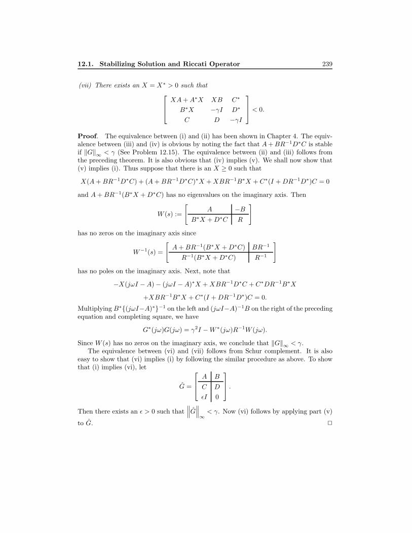
12.1. Stabilizing Solution and Riccati Operator 239
(vii) There exists an X = X∗ > 0 such that XA+A∗X XB C∗
B∗X −γI D∗
C D −γI
< 0.
Proof. The equivalence between (i) and (ii) has been shown in Chapter 4. The equiv-alence between (iii) and (iv) is obvious by noting the fact that A+BR−1D∗C is stableif ‖G‖∞ < γ (See Problem 12.15). The equivalence between (ii) and (iii) follows fromthe preceding theorem. It is also obvious that (iv) implies (v). We shall now show that(v) implies (i). Thus suppose that there is an X ≥ 0 such that
X(A+BR−1D∗C) + (A+BR−1D∗C)∗X +XBR−1B∗X + C∗(I +DR−1D∗)C = 0
and A+BR−1(B∗X +D∗C) has no eigenvalues on the imaginary axis. Then
W (s) :=
[A −B
B∗X +D∗C R
]has no zeros on the imaginary axis since
W−1(s) =
[A+BR−1(B∗X +D∗C) BR−1
R−1(B∗X +D∗C) R−1
]has no poles on the imaginary axis. Next, note that
−X(jωI −A)− (jωI −A)∗X +XBR−1D∗C + C∗DR−1B∗X
+XBR−1B∗X + C∗(I +DR−1D∗)C = 0.
Multiplying B∗(jωI−A)∗−1 on the left and (jωI−A)−1B on the right of the precedingequation and completing square, we have
G∗(jω)G(jω) = γ2I −W ∗(jω)R−1W (jω).
Since W (s) has no zeros on the imaginary axis, we conclude that ‖G‖∞ < γ.The equivalence between (vi) and (vii) follows from Schur complement. It is also
easy to show that (vi) implies (i) by following the similar procedure as above. To showthat (i) implies (vi), let
G =
A B
C D
εI 0
.Then there exists an ε > 0 such that
∥∥∥G∥∥∥∞< γ. Now (vi) follows by applying part (v)
to G. 2
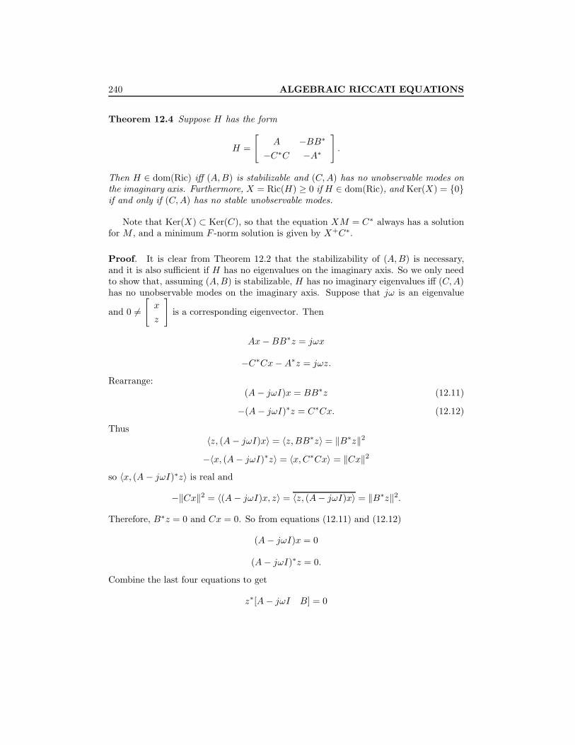
240 ALGEBRAIC RICCATI EQUATIONS
Theorem 12.4 Suppose H has the form
H =
[A −BB∗
−C∗C −A∗
].
Then H ∈ dom(Ric) iff (A,B) is stabilizable and (C,A) has no unobservable modes onthe imaginary axis. Furthermore, X = Ric(H) ≥ 0 if H ∈ dom(Ric), and Ker(X) = 0if and only if (C,A) has no stable unobservable modes.
Note that Ker(X) ⊂ Ker(C), so that the equation XM = C∗ always has a solutionfor M , and a minimum F -norm solution is given by X+C∗.
Proof. It is clear from Theorem 12.2 that the stabilizability of (A,B) is necessary,and it is also sufficient if H has no eigenvalues on the imaginary axis. So we only needto show that, assuming (A,B) is stabilizable, H has no imaginary eigenvalues iff (C,A)has no unobservable modes on the imaginary axis. Suppose that jω is an eigenvalue
and 0 6=[x
z
]is a corresponding eigenvector. Then
Ax−BB∗z = jωx
−C∗Cx−A∗z = jωz.
Rearrange:(A− jωI)x = BB∗z (12.11)
−(A− jωI)∗z = C∗Cx. (12.12)
Thus〈z, (A− jωI)x〉 = 〈z,BB∗z〉 = ‖B∗z‖2
−〈x, (A− jωI)∗z〉 = 〈x,C∗Cx〉 = ‖Cx‖2
so 〈x, (A − jωI)∗z〉 is real and
−‖Cx‖2 = 〈(A− jωI)x, z〉 = 〈z, (A− jωI)x〉 = ‖B∗z‖2.
Therefore, B∗z = 0 and Cx = 0. So from equations (12.11) and (12.12)
(A− jωI)x = 0
(A− jωI)∗z = 0.
Combine the last four equations to get
z∗[A− jωI B] = 0

12.1. Stabilizing Solution and Riccati Operator 241
[A− jωI
C
]x = 0.
The stabilizability of (A,B) gives z = 0. Now it is clear that jω is an eigenvalue of Hiff jω is an unobservable mode of (C,A).
Next, set X := Ric(H). We will show that X ≥ 0. The Riccati equation is
A∗X +XA−XBB∗X + C∗C = 0
or, equivalently,
(A−BB∗X)∗X +X(A−BB∗X) +XBB∗X + C∗C = 0. (12.13)
Noting that A−BB∗X is stable (Theorem 12.1), we have
X =∫ ∞
0
e(A−BB∗X)∗t(XBB∗X + C∗C)e(A−BB∗X)tdt. (12.14)
Since XBB∗X + C∗C is positive semidefinite, so is X .Finally, we will show that KerX is nontrivial if and only if (C,A) has stable unob-
servable modes. Let x ∈ KerX , then Xx = 0. Premultiply equation (12.13) by x∗ andpostmultiply by x to get
Cx = 0.
Now postmultiply equation (12.13) again by x to get
XAx = 0.
We conclude that Ker(X) is an A-invariant subspace. Thus if Ker(X) 6= 0, thenthere is a 0 6= x ∈ Ker(X) and a λ such that λx = Ax = (A − BB∗X)x and Cx =0. Since (A − BB∗X) is stable, Reλ < 0; thus λ is a stable unobservable mode.Conversely, suppose (C,A) has an unobservable stable mode λ (i.e., there is an x suchthat Ax = λx,Cx = 0). By premultiplying the Riccati equation by x∗ and post-multiplying by x, we get
2Reλx∗Xx− x∗XBB∗Xx = 0.
Hence x∗Xx = 0 (i.e., X is singular) since Reλ < 0. 2
Example 12.2 This example shows that the observability of (C,A) is not necessaryfor the existence of a positive definite stabilizing solution. Let
A =
[1 00 2
], B =
[11
], C =
[0 0
].

242 ALGEBRAIC RICCATI EQUATIONS
Then (A,B) is stabilizable, but (C,A) is not detectable. However,
X =
[18 −24−24 36
]> 0
is the stabilizing solution.
Corollary 12.5 Suppose that (A,B) is stabilizable and (C,A) is detectable. Then theRiccati equation
A∗X +XA−XBB∗X + C∗C = 0
has a unique positive semidefinite solution. Moreover, the solution is stabilizing.
Proof. It is obvious from the preceding theorem that the Riccati equation has a uniquestabilizing solution and that the solution is positive semidefinite. Hence we only needto show that any positive semidefinite solution X ≥ 0 must also be stabilizing. Thenby the uniqueness of the stabilizing solution, we can conclude that there is only onepositive semidefinite solution. To achieve that goal, let us assume that X ≥ 0 satisfiesthe Riccati equation but that it is not stabilizing. First rewrite the Riccati equation as
(A−BB∗X)∗X +X(A−BB∗X) +XBB∗X + C∗C = 0 (12.15)
and let λ and x be an unstable eigenvalue and the corresponding eigenvector ofA−BB∗X , respectively; that is,
(A−BB∗X)x = λx.
Now premultiply and postmultiply equation (12.15) by x∗ and x, respectively, and wehave
(λ+ λ)x∗Xx+ x∗(XBB∗X + C∗C)x = 0.
This impliesB∗Xx = 0, Cx = 0
since Re(λ) ≥ 0 and X ≥ 0. Finally, we arrive at
Ax = λx, Cx = 0.
That is, (C,A) is not detectable, which is a contradiction. Hence Re(λ) < 0 (i.e., X ≥ 0is the stabilizing solution). 2
Lemma 12.6 Suppose D has full column rank and let R = D∗D > 0; then the followingstatements are equivalent:
(i)
[A− jωI B
C D
]has full column rank for all ω.
(ii)((I −DR−1D∗)C, A−BR−1D∗C
)has no unobservable modes on the jω axis.

12.1. Stabilizing Solution and Riccati Operator 243
Proof. Suppose jω is an unobservable mode of((I −DR−1D∗)C, A−BR−1D∗C
);
then there is an x 6= 0 such that
(A−BR−1D∗C)x = jωx, (I −DR−1D∗)Cx = 0;
that is, [A− jωI B
C D
][I 0
−R−1D∗C I
][x
0
]= 0.
But this implies that [A− jωI B
C D
](12.16)
does not have full-column rank. Conversely, suppose equation (12.16) does not have
full-column rank for some ω; then there exists
[u
v
]6= 0 such that
[A− jωI B
C D
][u
v
]= 0.
Now let [u
v
]=
[I 0
−R−1D∗C I
][x
y
].
Then [x
y
]=
[I 0
R−1D∗C I
][u
v
]6= 0
and(A−BR−1D∗C − jωI)x+By = 0 (12.17)
(I −DR−1D∗)Cx+Dy = 0. (12.18)
Premultiply equation (12.18) by D∗ to get y = 0. Then we have
(A−BR−1D∗C)x = jωx, (I −DR−1D∗)Cx = 0;
that is, jω is an unobservable mode of((I −DR−1D∗)C, A−BR−1D∗C
). 2
Remark 12.2 If D is not square, then there is a D⊥ such that[D⊥ DR−1/2
]is
unitary and thatD⊥D∗⊥ = I−DR−1D∗. Hence, in some cases we will write the condition(ii) in the preceding lemma as (D∗⊥C,A−BR−1D∗C) having no imaginary unobservablemodes. Of course, if D is square, the condition is simplified to A−BR−1D∗C having noimaginary eigenvalues. Note also that if D∗C = 0, condition (ii) becomes (C,A) havingno imaginary unobservable modes. 3

244 ALGEBRAIC RICCATI EQUATIONS
Corollary 12.7 Suppose D has full column rank and denote R = D∗D > 0. Let Hhave the form
H =
[A 0
−C∗C −A∗
]−[
B
−C∗D
]R−1
[D∗C B∗
]=
[A−BR−1D∗C −BR−1B∗
−C∗(I −DR−1D∗)C −(A−BR−1D∗C)∗
].
Then H ∈ dom(Ric) iff (A,B) is stabilizable and
[A− jωI B
C D
]has full-column rank
for all ω. Furthermore, X = Ric(H) ≥ 0 if H ∈ dom(Ric), and Ker(X) = 0 if andonly if (D∗⊥C,A−BR−1D∗C) has no stable unobservable modes.
Proof. This is the consequence of Lemma 12.6 and Theorem 12.4. 2
Remark 12.3 It is easy to see that the detectability (observability) of(D∗⊥C,A−BR−1D∗C) implies the detectability (observability) of (C,A); however, theconverse is, in general, not true. Hence the existence of a stabilizing solution to theRiccati equation in the preceding corollary is not guaranteed by the stabilizability of(A,B) and detectability of (C,A). Furthermore, even if a stabilizing solution exists,the positive definiteness of the solution is not guaranteed by the observability of (C,A)unless D∗C = 0. As an example, consider
A =
[0 10 0
], B =
[0−1
], C =
[1 00 0
], D =
[10
].
Then (C,A) is observable, (A,B) is controllable, and
A−BD∗C =
[0 11 0
], D∗⊥C =
[0 0
].
A Riccati equation with the preceding data has a nonnegative definite stabilizing so-lution since (D∗⊥C,A −BR−1D∗C) has no unobservable modes on the imaginary axis.However, the solution is not positive definite since (D∗⊥C,A−BR−1D∗C) has a stableunobservable mode. On the other hand, if the B matrix is changed to
B =
[01
],
then the corresponding Riccati equation has no stabilizing solution since, in this case,(A−BD∗C) has eigenvalues on the imaginary axis although (A,B) is controllable and(C,A) is observable. 3
Related MATLAB Commands: ric eig, are

12.2. Inner Functions 245
12.2 Inner Functions
A transfer function N is called inner if N ∈ RH∞ and N∼N = I and co-inner ifN ∈ RH∞ and NN∼ = I. Note that N need not be square. Inner and co-inner aredual notions (i.e., N is an inner iff NT is a co-inner). A matrix function N ∈ RL∞ iscalled all-pass if N is square and N∼N = I; clearly a square inner function is all-pass.We will focus on the characterizations of inner functions here, and the properties ofco-inner functions follow by duality.
Note that N inner implies that N has at least as many rows as columns. ForN inner and any q ∈ Cm, v ∈ L2, ‖N(jω)q‖ = ‖q‖, ∀ω and ‖Nv‖2 = ‖v‖2 sinceN(jω)∗N(jω) = I for all ω. Because of these norm preserving properties, inner matriceswill play an important role in the control synthesis theory in this book. In this section,we present a state-space characterization of inner transfer functions.
Lemma 12.8 Suppose N =
[A B
C D
]∈ RH∞ and X = X∗ ≥ 0 satisfies
A∗X +XA+ C∗C = 0. (12.19)
Then
(a) D∗C + B∗X = 0 implies N∼N = D∗D.
(b) (A,B) is controllable, and N∼N = D∗D implies that D∗C +B∗X = 0.
Proof. Conjugating the states of
N∼N =
A 0 B
−C∗C −A∗ −C∗DD∗C B∗ D∗D
by
[I 0−X I
]on the left and
[I 0−X I
]−1
=
[I 0X I
]on the right yields
N∼N =
A 0 B
−(A∗X +XA+ C∗C) −A∗ −(XB + C∗D)
B∗X +D∗C B∗ D∗D
=
A 0 B
0 −A∗ −(XB + C∗D)
B∗X +D∗C B∗ D∗D
.Then (a) and (b) follow easily. 2

246 ALGEBRAIC RICCATI EQUATIONS
This lemma immediately leads to one characterization of inner matrices in termsof their state-space representations. Simply add the condition that D∗D = I toLemma 12.8 to get N∼N = I.
Corollary 12.9 Suppose N =
[A B
C D
]is stable and minimal, and X is the observ-
ability Gramian. Then N is an inner if and only if
(a) D∗C + B∗X = 0
(b) D∗D = I.
A transfer matrix N⊥ is called a complementary inner factor (CIF) of N if [N N⊥]is square and is an inner. The dual notion of the complementary co-inner factor isdefined in the obvious way. Given an inner N , the following lemma gives a constructionof its CIF. The proof of this lemma follows from straightforward calculation and fromthe fact that CX+X = C since Im(I −X+X) ⊂ Ker(X) ⊂ Ker(C).
Lemma 12.10 Let N =
[A B
C D
]be an inner and X be the observability Gramian.
Then a CIF N⊥ is given by
N⊥ =
[A −X+C∗D⊥
C D⊥
]
where D⊥ is an orthogonal complement of D such that [D D⊥] is square and orthogonal.
12.3 Notes and References
The general solutions of a Riccati equation are given by Martensson [1971]. The paper byWillems [1971] contains a comprehensive treatment of ARE and the related optimizationproblems. Some matrix factorization results are given in Doyle [1984]. Numericalmethods for solving ARE can be found in Arnold and Laub [1984], Van Dooren [1981],and references therein. See Zhou, Doyle, and Glover [1996] and Lancaster and Rodman[1995] for a more extensive treatment of this subject.
12.4 Problems
Problem 12.1 Assume that G(s) :=
[A B
C D
]∈ RL∞ is a stabilizable and de-
tectable realization and γ > ‖G(s)‖∞. Show that there exists a transfer matrix M ∈

12.4. Problems 247
RL∞ such that M∼M = γ2I −G∼G and M−1 ∈ RH∞. A particular realization of Mis
M(s) =
[A B
−R1/2F R1/2
]where
R = γ2I −D∗DF = R−1(B∗X +D∗C)
X = Ric
[A+BR−1D∗C BR−1B∗
−C∗(I +DR−1D∗)C −(A+BR−1D∗C)∗
]and X ≥ 0 if A is stable.
Problem 12.2 Let G(s) =
[A B
C D
]be a stabilizable and detectable realization.
Suppose G∼(jω)G(jω) > 0 for all ω or
[A− jω B
C D
]has full-column rank for all ω.
Let
X = Ric
[A−BR−1D∗C −BR−1B∗
−C∗(I −DR−1D∗)C −(A−BR−1D∗C)∗
]with R := D∗D > 0. Show
W∼W = G∼G
where W−1 ∈ RH∞ and
W =
[A B
R−1/2(D∗C +B∗X) R1/2
].
Problem 12.3 A square (m×m) matrix function G(s) ∈ RH∞ is said to be positivereal (PR) if G(jω) +G∗(jω) ≥ 0 for all finite ω; and G(s) is said to be strictly positive
real (SPR) if G(jω) + G∗(jω) > 0 for all ω ∈ R. Let
[A B
C D
]be a state-space
realization of G(s) with A stable (not necessarily a minimal realization). Suppose thereexist X ≥ 0, Q, and W such that
XA+A∗X = −Q∗Q (12.20)B∗X +W ∗Q = C (12.21)
D +D∗ = W ∗W, (12.22)
Show that G(s) is positive real and
G(s) +G∼(s) = M∼(s)M(s)

248 ALGEBRAIC RICCATI EQUATIONS
with M(s) =
[A B
Q W
]. Furthermore, if M(jω) has full-column rank for all ω ∈ R,
then G(s) is strictly positive real.
Problem 12.4 Suppose (A,B,C,D) is a minimal realization of G(s) with A stable andG(s) positive real. Show that there exist X ≥ 0, Q, and W such that
XA+A∗X = −Q∗QB∗X +W ∗Q = C
D +D∗ = W ∗W
andG(s) +G∼(s) = M∼(s)M(s)
with M(s) =
[A B
Q W
]. Furthermore, if G(s) is strictly positive real, then M(jω) has
full-column rank for all ω ∈ R.
Problem 12.5 Let
[A B
C D
]be a state-space realization of G(s) ∈ RH∞ with A
stable and R := D+D∗ > 0. Show that G(s) is strictly positive real if and only if thereexists a stabilizing solution to the following Riccati equation:
X(A−BR−1C) + (A−BR−1C)∗X +XBR−1B∗X + C∗R−1C = 0.
Moreover, M(s) =
[A B
R−12 (C −B∗X) R
12
]is minimal phase and
G(s) +G∼(s) = M∼(s)M(s).
Problem 12.6 Assume p ≥ m. Show that there exists an rcf G = NM−1 such that Nis an inner if and only if G∼G > 0 on the jω axis, including at∞. This factorization isunique up to a constant unitary multiple. Furthermore, assume that the realization of
G =
[A B
C D
]is stabilizable and that
[A− jωI B
C D
]has full column rank for all
ω ∈ R. Then a particular realization of the desired coprime factorization is
[M
N
]:=
A+BF BR−1/2
F
C +DF
R−1/2
DR−1/2
∈ RH∞where
R = D∗D > 0

12.4. Problems 249
F = −R−1(B∗X +D∗C)
and
X = Ric
[A−BR−1D∗C −BR−1B∗
−C∗(I −DR−1D∗)C −(A−BR−1D∗C)∗
]≥ 0.
Moreover, a complementary inner factor can be obtained as
N⊥ =
[A+BF −X†C∗D⊥C +DF D⊥
]
if p > m.
Problem 12.7 Assume that G =
[A B
C D
]∈ Rp(s) and (A,B) is stabilizable. Show
that there exists a right coprime factorization G = NM−1 such that M ∈ RH∞ is aninner if and only if G has no poles on the jω axis. A particular realization is
[M
N
]:=
A+BF B
F
C +DF
I
D
∈ RH∞where
F = −B∗X
X = Ric
[A −BB∗
0 −A∗
]≥ 0.
Problem 12.8 A right coprime factorization of G = NM−1 with N,M ∈ RH∞ is
called a normalized right coprime factorization if M∼M +N∼N = I; that is, if
[M
N
]is an inner. Similarly, an lcf G = M−1N is called a normalized left coprime factorization
if[M N
]is a co-inner. Let a realization of G be given by G =
[A B
C D
]and define
R = I +D∗D > 0 and R = I +DD∗ > 0.
(a) Suppose (A,B) is stabilizable and (C,A) has no unobservable modes on the imagi-nary axis. Show that there is a normalized right coprime factorizationG = NM−1
[M
N
]:=
A+BF BR−1/2
F
C +DF
R−1/2
DR−1/2
∈ RH∞

250 ALGEBRAIC RICCATI EQUATIONS
whereF = −R−1(B∗X +D∗C)
and
X = Ric
[A−BR−1D∗C −BR−1B∗
−C∗R−1C −(A−BR−1D∗C)∗
]≥ 0.
(b) Suppose (C,A) is detectable and (A,B) has no uncontrollable modes on the imag-inary axis. Show that there is a normalized left coprime factorization G = M−1N
[M N
]:=
[A+ LC L B + LD
R−1/2C R−1/2 R−1/2D
]
whereL = −(BD∗ + Y C∗)R−1
and
Y = Ric
[(A−BD∗R−1C)∗ −C∗R−1C
−BR−1B∗ −(A−BD∗R−1C)
]≥ 0.
(c) Show that the controllability Gramian P and the observability Gramian Q of[M
N
]are given by
P = (I + Y X)−1Y, Q = X
while the controllability Gramian P and observability Gramian Q of[M N
]are given by
P = Y, Q = (I +XY )−1X.
Problem 12.9 Let G(s) =
[A B
C D
]. Find M1 andM2 such that M−1
1 ,M−12 ∈ RH∞
andM1M
∼1 = I +GG∼, M∼2 M2 = I +G∼G.
Problem 12.10 Let A ∈ Rm×m, B ∈ Rn×n, C ∈ Rm×n, and consider the Sylvesterequation
AX +XB = C
for an unknown matrix X ∈ Rm×n. Let
M =
[B 0C −A
], N =
[B 00 −A
].

12.4. Problems 251
1. Let the columns of
[U
V
]∈ Cn+m×n be the eigenvectors of M associated with
the eigenvalues of B and suppose U is nonsingular. Show that
X = V U−1
solves the Sylvester equation. Moreover, every solution of the Sylvester equationcan be written in the above form.
2. Show that the Sylvester equation has a solution if and only if M and N are similar.(See Lancaster and Tismenetsky [1985, page 423].)
Problem 12.11 Let A ∈ Rn×n. Show that
P (t) =∫ t
0
eA∗τQeAτdτ
satisfiesP (t) = A∗P (t) + P (t)A+Q, P (0) = 0.
Problem 12.12 A more general case of the above problem is when the given matricesare time varying and the initial condition is not zero. Let A(t), Q(t), P0 ∈ Rn×n. Showthat
P (t) = ΦT (t, t0)P0Φ(t, t0) +∫ t
t0
ΦT (t, τ)Q(τ)Φ(t, τ)dτ
satisfiesP (t) = A∗P (t) + P (t)A+Q(t), P (t0) = P0
where Φ(t, τ) is the state transition matrix for the system x = A(t)x.
Problem 12.13 Let A ∈ Rn×n, R = R∗, Q = Q∗. Define
H =
[A R
−Q −A∗
].
Let
Θ(t) =
[Θ11(t) Θ12(t)Θ21(t) Θ22(t)
]= eHt.
Show thatP (t) = (Θ21(t) + Θ22P0)(Θ11(t) + Θ12(t)P0)−1
is the solution to the following differential Riccati equation:
−P (t) = A∗P (t) + P (t)A+ PRP +Q, P (0) = P0.

252 ALGEBRAIC RICCATI EQUATIONS
Problem 12.14 Let A ∈ Rn×n, R = R∗, Q = Q∗. Define
H =
[A R
−Q −A∗
].
Let
Θ(t) =
[Θ11(t) Θ12(t)Θ21(t) Θ22(t)
]= eH(t−T ).
Show thatP (t) = Θ21(t)Θ−1
11 (t)
is the solution to the following differential Riccati equation:
−P (t) = A∗P (t) + P (t)A+ PRP +Q, P (T ) = 0.
Problem 12.15 Suppose G(s) =
[A B
C D
]∈ RH∞ and ‖G‖∞ < γ. Show that
A+BR−1D∗C with R = γ2I −D∗D is stable. (Hint: Show A+B(I −∆D/γ)−1∆C/γis stable for all ∆ with ‖∆‖ ≤ 1.)

Chapter 13
H2 Optimal Control
In this chapter we treat the optimal control of linear time-invariant systems with aquadratic performance criterion.
13.1 Introduction to Regulator Problem
Consider the following dynamical system:
x = Ax+ B2u, x(t0) = x0 (13.1)
where x0 is given but arbitrary. Our objective is to find a control function u(t) definedon [t0, T ], which can be a function of the state x(t), such that the state x(t) is driven toa (small) neighborhood of origin at time T . This is the so-called regulator problem. Onemight suggest that this regulator problem can be trivially solved for any T > t0 if thesystem is controllable. This is indeed the case if the controller can provide arbitrarilylarge amount of energy since, by the definition of controllability, one can immediatelyconstruct a control function that will drive the state to zero in an arbitrarily shorttime. However, this is not practical since any physical system has energy limitation(i.e., the actuator will eventually saturate). Furthermore, large control action can easilydrive the system out of the region, where the given linear model is valid. Hence certainlimitations have to be imposed on the control in practical engineering implementation.The constraints on control u may be measured in many different ways; for example,∫ T
t0
‖u‖ dt,∫ T
t0
‖u‖2 dt, supt∈[t0,T ]
‖u‖ ;
That is, in terms of L1 norm, L2 norm, and L∞ norm or, more generally, weighted L1
norm, L2 norm, and L∞ norm∫ T
t0
‖Wuu‖ dt,∫ T
t0
‖Wuu‖2 dt, supt∈[t0,T ]
‖Wuu‖
253

254 H2 OPTIMAL CONTROL
for some constant weighting matrix Wu.Similarly, one might also want to impose some constraints on the transient response
x(t) in a similar fashion:∫ T
t0
‖Wxx‖ dt,∫ T
t0
‖Wxx‖2 dt, supt∈[t0,T ]
‖Wxx‖
for some weighting matrix Wx. Hence the regulator problem can be posed as an optimalcontrol problem with certain combined performance index on u and x. In this chap-ter, we shall be concerned exclusively with the L2 performance problem or quadraticperformance problem. Moreover, we shall focus on the infinite time regulator problem(i.e., T →∞) and, without loss of generality, we shall assume t0 = 0. In this case, ourproblem is as follows: Find a control u(t) defined on [0,∞) such that the state x(t) isdriven to the origin as t→∞ and the following performance index is minimized:
minu
∫ ∞0
[x(t)u(t)
]∗ [Q S
S∗ R
][x(t)u(t)
]dt (13.2)
for some Q = Q∗, S, and R = R∗ > 0. This problem is traditionally called a linearquadratic regulator problem or, simply, an LQR problem. Here we have assumed R > 0to emphasize that the control energy has to be finite (i.e., u(t) ∈ L2[0,∞)). So L2[0,∞)is the space over which the integral is minimized. Moreover, it is also generally assumedthat [
Q S
S∗ R
]≥ 0. (13.3)
Since R is positive definite, it has a square root, R1/2, which is also positive-definite.By the substitution
u← R1/2u,
we may as well assume at the start that R = I. In fact, we can even assume S = 0by using a pre-state feedback u = −S∗x+ v provided some care is exercised; however,this will not be assumed in the sequel. Since the matrix in equation (13.3) is positivesemi-definite with R = I, it can be factored as[
Q S
S∗ I
]=
[C∗1D∗12
] [C1 D12
].
Then equation (13.2) can be rewritten as
minu∈L2[0,∞)
‖C1x+D12u‖22 .

13.2. Standard LQR Problem 255
In fact, the LQR problem is posed traditionally as the minimization problem:
minu∈L2[0,∞)
‖C1x+D12u‖22 (13.4)
subject to: x = Ax+Bu, x(0) = x0 (13.5)
without explicitly mentioning the condition that the control should drive the state to theorigin. Instead some assumptions are imposed on Q,S, and R (or, equivalently, on C1
andD12) to ensure that the optimal control law u has this property. To see what assump-tion one needs to make to ensure that the minimization problem formulated in equations(13.4) and (13.5) has a sensible solution, let us consider a simple example with A = 1,B = 1, Q = 0, S = 0, and R = 1:
minu∈L2[0,∞)
∫ ∞0
u2dt, x = x+ u, x(0) = x0.
It is clear that u = 0 is the optimal solution. However, the system with u = 0 isunstable and x(t) diverges exponentially to infinity since x(t) = etx0. The problemwith this example is that this performance index does not “see” the unstable state x.Thus, to ensure that the minimization problem in equations (13.4) and (13.5) is sensible,we must assume that all unstable states can be “seen” from the performance index; thatis, (C1, A) must be detectable. An LQR problem with such an assumption will be calleda standard LQR problem.
On the other hand, if the closed-loop stability is imposed on the preceding mini-mization, then it can be shown that minu∈L2[0,∞)
∫∞0 u2dt = 2x2
0 and u(t) = −2x(t) isthe optimal control. This can also be generalized to a more general case where (C1, A)is not necessarily detectable. Such a LQR problem will be referred to as an ExtendedLQR problem.
13.2 Standard LQR Problem
In this section, we shall consider the LQR problem as traditionally formulated.
Standard LQR Problem
Let a dynamical system be described by
x = Ax+B2u, x(0) = x0 given but arbitrary (13.6)z = C1x+D12u (13.7)
and suppose that the system parameter matrices satisfy the following as-sumptions:
(A1) (A,B2) is stabilizable;
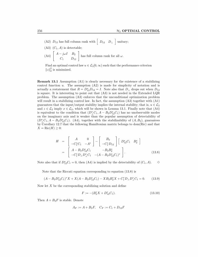
256 H2 OPTIMAL CONTROL
(A2) D12 has full column rank with[D12 D⊥
]unitary;
(A3) (C1, A) is detectable;
(A4)
[A− jωI B2
C1 D12
]has full column rank for all ω.
Find an optimal control law u ∈ L2[0,∞) such that the performance criterion‖z‖22 is minimized.
Remark 13.1 Assumption (A1) is clearly necessary for the existence of a stabilizingcontrol function u. The assumption (A2) is made for simplicity of notation and isactually a restatement that R = D∗12D12 = I. Note also that D⊥ drops out when D12
is square. It is interesting to point out that (A3) is not needed in the Extended LQRproblem. The assumption (A3) enforces that the unconditional optimization problemwill result in a stabilizing control law. In fact, the assumption (A3) together with (A1)guarantees that the input/output stability implies the internal stability; that is, u ∈ L2
and z ∈ L2 imply x ∈ L2, which will be shown in Lemma 13.1. Finally note that (A4)is equivalent to the condition that (D∗⊥C1, A − B2D
∗12C1) has no unobservable modes
on the imaginary axis and is weaker than the popular assumption of detectability of(D∗⊥C1, A − B2D
∗12C1). (A4), together with the stabilizability of (A,B2), guarantees
by Corollary 12.7 that the following Hamiltonian matrix belongs to dom(Ric) and thatX = Ric(H) ≥ 0:
H =
[A 0
−C∗1C1 −A∗
]−[
B2
−C∗1D12
] [D∗12C1 B∗2
]=
[A−B2D
∗12C1 −B2B
∗2
−C∗1D⊥D∗⊥C1 −(A−B2D∗12C1)∗
]. (13.8)
Note also that if D∗12C1 = 0, then (A4) is implied by the detectability of (C1, A). 3
Note that the Riccati equation corresponding to equation (13.8) is
(A−B2D∗12C1)∗X +X(A−B2D
∗12C1)−XB2B
∗2X + C∗1D⊥D
∗⊥C1 = 0. (13.9)
Now let X be the corresponding stabilizing solution and define
F := −(B∗2X +D∗12C1). (13.10)
Then A+ B2F is stable. Denote
AF := A+B2F, CF := C1 +D12F

13.2. Standard LQR Problem 257
and rearrange equation (13.9) to get
A∗FX +XAF + C∗FCF = 0. (13.11)
Thus X is the observability Gramian of (CF , AF ).Consider applying the control law u = Fx to the system equations (13.6) and (13.7).
The controlled system becomes
x = AFx, x(0) = x0
z = CFx
or, equivalently,
x = AFx+ x0δ(t), x(0−) = 0z = CFx.
The associated transfer matrix is
Gc(s) =
[AF I
CF 0
]and
‖Gcx0‖22 = x∗0Xx0.
The proof of the following theorem requires a preliminary result about internalstability given input-output stability.
Lemma 13.1 If u, z ∈ L2[0,∞) and (C1, A) is detectable in the system described byequations (13.6) and (13.7), then x ∈ L2[0,∞). Furthermore, x(t)→ 0 as t→∞.
Proof. Since (C1, A) is detectable, there exists L such that A+ LC1 is stable. Let xbe the state estimate of x given by
˙x = (A+ LC1)x+ (LD12 +B2)u− Lz.
Then x ∈ L2[0,∞) and x → 0 (see Problem 13.1) since z and u are in L2[0,∞). Nowlet e = x− x; then
e = (A+ LC1)e
and e ∈ L2[0,∞). Therefore, x = e + x ∈ L2[0,∞). It is easy to see that e(t) → 0 ast→∞ for any initial condition e(0). Finally, x(t)→ 0 since x→ 0. 2
Theorem 13.2 There exists a unique optimal control for the LQR problem, namelyu = Fx. Moreover,
minu∈L2[0,∞)
‖z‖2 = ‖Gcx0‖2 .
Note that the optimal control strategy is a constant gain state feedback, and thisgain is independent of the initial condition x0.

258 H2 OPTIMAL CONTROL
Proof. With the change of variable v = u− Fx, the system can be written as[x
z
]=
[AF B2
CF D12
][x
v
], x(0) = x0. (13.12)
Now if v ∈ L2[0,∞), then x, z ∈ L2[0,∞) and x(∞) = 0 since AF is stable.Hence u = Fx + v ∈ L2[0,∞). Conversely, if u, z ∈ L2[0,∞), then from Lemma 13.1x ∈ L2[0,∞). So v ∈ L2[0,∞). Thus the mapping v = u − Fx between v ∈ L2[0,∞)and those u ∈ L2[0,∞) that make z ∈ L2[0,∞) is one-to-one and onto. Therefore,
minu∈L2[0,∞)
‖z‖2 = minv∈L2[0,∞)
‖z‖2 .
By differentiating x(t)∗Xx(t) with respect to t along a solution of the differential equa-tion (13.12) and by using equation (13.9) and the fact that C∗FD12 = −XB2, we seethat
d
dtx∗Xx = x∗Xx+ x∗Xx = x∗(A∗FX +XAF )x+ 2x∗XB2v
= −x∗C∗FCFx+ 2x∗XB2v
= −(CFx+D12v)∗(CFx+D12v) + 2x∗C∗FD12v + v∗v + 2x∗XB2v
= −‖z‖2 + ‖v‖2 . (13.13)
Now integrate equation (13.13) from 0 to ∞ to get
‖z‖22 = x∗0Xx0 + ‖v‖22 .
Clearly, the unique optimal control is v = 0, i.e., u = Fx. 2
13.3 Extended LQR Problem
This section considers the extended LQR problem where no detectability assumption ismade for (C1, A).
Extended LQR Problem
Let a dynamical system be given by
x = Ax+B2u, x(0) = x0 given but arbitraryz = C1x+D12u
with the following assumptions:
(A1) (A,B2) is stabilizable;

13.4. Guaranteed Stability Margins of LQR 259
(A2) D12 has full column rank with[D12 D⊥
]unitary;
(A3)
[A− jωI B2
C1 D12
]has full column rank for all ω.
Find an optimal control law u ∈ L2[0,∞) such that the system is internallystable (i.e., x ∈ L2[0,∞)) and the performance criterion ‖z‖22 is minimized.
Assume the same notation as in the last section, we have:
Theorem 13.3 There exists a unique optimal control for the extended LQR problem,namely u = Fx. Moreover,
minu∈L2[0,∞)
‖z‖2 = ‖Gcx0‖2 .
Proof. The proof of this theorem is very similar to the proof of the standard LQRproblem except that, in this case, the input/output stability may not necessarily implythe internal stability. Instead, the internal stability is guaranteed by the way of choosingcontrol law.
Suppose that u ∈ L2[0,∞) is such a control law that the system is stable, i.e.,x ∈ L2[0,∞). Then v = u − Fx ∈ L2[0,∞). On the other hand, let v ∈ L2[0,∞) andconsider [
x
z
]=
[AF B2
CF D12
][x
v
], x(0) = x0.
Then x, z ∈ L2[0,∞) and x(∞) = 0 since AF is stable. Hence u = Fx+ v ∈ L2[0,∞).Again the mapping v = u−Fx between v ∈ L2[0,∞) and those u ∈ L2[0,∞) that makez ∈ L2[0,∞) and x ∈ L2[0,∞) is one to one and onto. Therefore,
minu∈L2[0,∞)
‖z‖2 = minv∈L2[0,∞)
‖z‖2 .
Using the same technique as in the proof of the standard LQR problem, we have
‖z‖22 = x∗0Xx0 + ‖v‖22 .Thus, the unique optimal control is v = 0, i.e., u = Fx. 2
13.4 Guaranteed Stability Margins of LQR
Now we will consider the system described by equation (13.6) with the LQR control lawu = Fx. The closed-loop block diagram is as shown in Figure 13.1.
The following result is the key to stability margins of an LQR control law.
Lemma 13.4 Let F = −(B∗2X + D∗12C1) and define G12 = D12 + C1(sI − A)−1B2.Then (
I −B∗2(−sI −A∗)−1F ∗) (I − F (sI −A)−1B2
)= G∼12(s)G12(s).

260 H2 OPTIMAL CONTROL
xu- -- x = Ax+B2uF
Figure 13.1: LQR closed-loop system
Proof. Note that the Riccati equation (13.9) can be written as
XA+A∗X − F ∗F + C∗1C1 = 0.
Add and subtract sX to the above equation to get
−X(sI − A)− (−sI −A∗)X − F ∗F + C∗1C1 = 0.
Now multiply the above equation from the left by B∗2(−sI −A∗)−1 and from the rightby (sI −A)−1B2 to get
−B∗2(−sI −A∗)−1XB2 −B∗2X(sI −A)−1B2 −B∗2(−sI −A∗)−1F ∗F (sI −A)−1B2
+B∗2(−sI −A∗)−1C∗1C1(sI −A)−1B2 = 0.
Using −B∗2X = F +D∗12C1 in the above equation, we have
B∗2(−sI −A∗)−1F ∗ + F (sI −A)−1B2 −B∗2 (−sI −A∗)−1F ∗F (sI −A)−1B2
+B∗2(−sI −A∗)−1C∗1D12 +D∗12C1(sI −A)−1B2
+B∗2(−sI −A∗)−1C∗1C1(sI −A)−1B2 = 0.
Then the result follows from completing the square and from the fact that D∗12D12 = I.2
Corollary 13.5 Suppose D∗12C1 = 0. Then(I −B∗2(−sI −A∗)−1F ∗
) (I − F (sI −A)−1B2
)= I+B∗2(−sI−A∗)−1C∗1C1(sI−A)−1B2.
In particular, (I −B∗2(−jωI −A∗)−1F ∗
) (I − F (jωI −A)−1B2
)≥ I (13.14)
and (I +B∗2 (−jωI −A∗ − F ∗B∗2)−1F ∗
) (I + F (jωI −A−B2F )−1B2
)≤ I. (13.15)

13.5. Standard H2 Problem 261
Note that the inequality (13.15) follows from taking the inverse of inequality (13.14).
Define G(s) = −F (sI − A)−1B2 and assume for the moment that the system issingle-input. Then the inequality (13.14) shows that the open-loop Nyquist diagramof the system G(s) in Figure 13.1 never enters the unit disk centered at (−1, 0) of thecomplex plane. Hence the system has at least a 6 dB (= 20 log 2) gain margin and a60o phase margin in both directions. A similar interpretation may be generalized tomultiple-input systems.
Next, it is noted that the inequality (13.15) can also be given some robustnessinterpretation. In fact, it implies that the closed-loop system in Figure 13.1 is stableeven if the open-loop system G(s) is perturbed additively by a ∆ ∈ RH∞ as long as‖∆‖∞ < 1. This can be seen from the following block diagram and the small gaintheorem, where the transfer matrix from w to z is exactly I +F (jωI −A−B2F )−1B2.
ez w
?
-
- --
∆
- x = Ax+B2uF
13.5 Standard H2 Problem
The system considered in this section is described by the following standard blockdiagram:
G
K
z
y
w
u
-
The realization of the transfer matrix G is taken to be of the form
G(s) =
A B1 B2
C1 0 D12
C2 D21 0
.Notice the special off-diagonal structure of D: D22 is assumed to be zero so that G22
is strictly proper;1 also, D11 is assumed to be zero in order to guarantee that the H2
1This assumption is made without loss of generality since a substitution of KD = K(I +D22K)−1
would give the controller for D22 6= 0.

262 H2 OPTIMAL CONTROL
problem is properly posed.2
The following additional assumptions are made for the output feedback H2 problemin this chapter:
(i) (A,B2) is stabilizable and (C2, A) is detectable;
(ii) R1 = D∗12D12 > 0 and R2 = D21D∗21 > 0;
(iii)
[A− jωI B2
C1 D12
]has full column rank for all ω;
(iv)
[A− jωI B1
C2 D21
]has full row rank for all ω.
The first assumption is for the stabilizability of G by output feedback, and the third andthe fourth assumptions together with the first guarantee that the two Hamiltonian ma-trices associated with the following H2 problem belong to dom(Ric). The assumptionsin (ii) guarantee that the H2 optimal control problem is nonsingular.
H2 Problem The H2 control problem is to find a proper, real rationalcontroller K that stabilizes G internally and minimizes the H2 norm of thetransfer matrix Tzw from w to z.
In the following discussions we shall assume that we have state models of G and K.Recall that a controller is said to be admissible if it is internally stabilizing and proper.By Corollary 12.7 the two Hamiltonian matrices
H2 :=
[A−B2R
−11 D∗12C1 −B2R
−11 B∗2
−C∗1 (I −D12R−11 D∗12)C1 −(A−B2R
−11 D∗12C1)∗
]
J2 :=
[(A−B1D
∗21R
−12 C2)∗ −C∗2R−1
2 C2
−B1(I −D∗21R−12 D21)B∗1 −(A−B1D
∗21R
−12 C2)
]belong to dom(Ric), and, moreover, X2 := Ric(H2) ≥ 0 and Y2 := Ric(J2) ≥ 0. Define
F2 := −R−11 (B∗2X2 +D∗12C1), L2 := −(Y2C
∗2 +B1D
∗21)R−1
2
andAF2 := A+B2F2, C1F2 := C1 +D12F2
AL2 := A+ L2C2, B1L2 := B1 + L2D21
A2 := A+B2F2 + L2C2
Gc(s) :=
[AF2 I
C1F2 0
], Gf (s) :=
[AL2 B1L2
I 0
].
Before stating the main theorem, we note the following fact:2Recall that a rational proper stable transfer function is an RH2 function iff it is strictly proper.

13.5. Standard H2 Problem 263
Lemma 13.6 Let U, V ∈ RH∞ be defined as
U :=
[AF2 B2R
−1/21
C1F2 D12R−1/21
], V :=
[AL2 B1L2
R−1/22 C2 R
−1/22 D21
].
Then U is an inner and V is a co-inner, U∼Gc ∈ RH⊥2 , and GfV ∼ ∈ RH⊥2 .
Proof. The proof uses standard manipulations of state-space realizations. From U weget
U∼(s) =
[−A∗F2
−C∗1F2
R−1/21 B∗2 R
−1/21 D∗12
].
Then it is easy to compute
U∼U =
−A∗F2−C∗1F2
C1F2 −C∗1F2D12R
−1/21
0 AF2 B2R−1/21
R−1/21 B∗2 R
−1/21 D∗12C1F2 I
U∼Gc =
−A∗F2−C∗1F2
C1F2 00 AF2 I
R−1/21 B∗2 R
−1/21 D∗12C1F2 0
.Now do the similarity transformation[
I −X2
0 I
]
on the states of the preceding transfer matrices and note that
A∗F2X2 +X2AF2 + C∗1F2
C1F2 = 0.
We get
U∼U =
−A∗F20 0
0 AF2 B2R−1/21
R−1/21 B∗2 0 I
= I
U∼Gc =
−A∗F20 −X2
0 AF2 I
R−1/21 B∗2 0 0
=
[−A∗F2
−X2
R−1/21 B∗2 0
]∈ RH⊥2 .
It follows by duality that GfV ∼ ∈ RH⊥2 and V is a co-inner. 2

264 H2 OPTIMAL CONTROL
Theorem 13.7 There exists a unique optimal controller
Kopt(s) :=
[A2 −L2
F2 0
].
Moreover,
min ‖Tzw‖22 = ‖GcB1‖22 + ‖R1/21 F2Gf‖22 = trace (B∗1X2B1) + trace (R1F2Y2F
∗2 ) .
Proof. Consider the all-stabilizing controller parameterization K(s) = F`(M2, Q),Q ∈ RH∞ with
M2(s) =
A2 −L2 B2
F2 0 I
−C2 I 0
and consider the following system diagram:
u1y1
y u
wz
-
XXXXXXX
Q
M2
G
Then Tzw = F`(N,Q) with
N =
AF2 −B2F2 B1 B2
0 AL2 B1L2 0
C1F2 −D12F2 0 D12
0 C2 D21 0
and
Tzw = GcB1 − UR1/21 F2Gf + UR
1/21 QR
1/22 V.
It follows from Lemma 13.6 that GcB1 and U are orthogonal. Thus
‖Tzw‖22 = ‖GcB1‖22 +∥∥∥UR1/2
1 F2Gf − UR1/21 QR
1/22 V
∥∥∥2
2
= ‖GcB1‖22 +∥∥∥R1/2
1 F2Gf −R1/21 QR
1/22 V
∥∥∥2
2.

13.6. Stability Margins of H2 Controllers 265
Since Gf and V are also orthogonal by Lemma 13.6, we have
‖Tzw‖22 = ‖GcB1‖22 +∥∥∥R1/2
1 F2Gf −R1/21 QR
1/22 V
∥∥∥2
2
= ‖GcB1‖22 +∥∥∥R1/2
1 F2Gf
∥∥∥2
2+∥∥∥R1/2
1 QR1/22
∥∥∥2
2.
This shows clearly that Q = 0 gives the unique optimal control, so K = F`(M2, 0) isthe unique optimal controller. 2
The optimal H2 controller, Kopt, and the closed-loop transfer matrix, Tzw, can beobtained by the following Matlab program:
[K,Tzw] = h2syn(G,ny,nu)
where ny and nu are the dimensions of y and u, respectively.
Related MATLAB Commands: lqg, lqr, lqr2, lqry, reg, lqe
13.6 Stability Margins of H2 Controllers
It is well-known that a system with LQR controller has at least 60o phase marginand 6 dB gain margin. However, it is not clear whether these stability margins willbe preserved if the states are not available and the output feedback H2 (or LQG)controller has to be used. The answer is provided here through a counterexample fromDoyle [1978]: There are no guaranteed stability margins for a H2 controller.
Consider a single-input and single-output two-state generalized dynamical system:
G(s) =
[1 10 1
] [ √σ 0√σ 0
] [01
][ √
q√q
0 0
]0
[01
][
1 0] [
0 1]
0
.
It can be shown analytically that
X2 =
[2α α
α α
], Y2 =
[2β β
β β
]
and
F2 = −α[
1 1], L2 = −β
[11
]

266 H2 OPTIMAL CONTROL
whereα = 2 +
√4 + q , β = 2 +
√4 + σ.
Then the optimal output H2 controller is given by
Kopt =
1− β 1 β
−(α+ β) 1− α β
−α −α 0
.Suppose that the resulting closed-loop controller (or plant G22) has a scalar gain k witha nominal value k = 1. Then the controller implemented in the system is actually
K = kKopt,
and the closed-loop system A matrix becomes
A =
1 1 0 00 1 −kα −kαβ 0 1− β 1β 0 −α− β 1− α
.It can be shown that the characteristic polynomial has the form
det(sI − A) = s4 + a3s3 + a2s
2 + a1s+ a0
witha1 = α+ β − 4 + 2(k − 1)αβ, a0 = 1 + (1− k)αβ.
Note that for closed-loop stability it is necessary to have a0 > 0 and a1 > 0. Note alsothat a0 ≈ (1 − k)αβ and a1 ≈ 2(k − 1)αβ for sufficiently large α and β if k 6= 1. It iseasy to see that for sufficiently large α and β (or q and σ), the system is unstable forarbitrarily small perturbations in k in either direction. Thus, by choice of q and σ, thegain margins may be made arbitrarily small.
It is interesting to note that the margins deteriorate as control weight (1/q) getssmall (large q) and/or system driving noise gets large (large σ). In modern controlfolklore, these have often been considered ad hoc means of improving sensitivity.
It is also important to recognize that vanishing margins are not only associated withopen-loop unstable systems. It is easy to construct minimum phase, open-loop stablecounterexamples for which the margins are arbitrarily small.
The point of this example is that H2 (LQG) solutions, unlike LQR solutions, pro-vide no global system-independent guaranteed robustness properties. Like their moreclassical colleagues, modern LQG designers are obliged to test their margins for eachspecific design.
It may, however, be possible to improve the robustness of a given design by relaxingthe optimality of the filter with respect to error properties. A successful approach in

13.7. Notes and References 267
this direction is the so called LQG loop transfer recovery (LQG/LTR) design technique.The idea is to design a filtering gain, L2, in such way so that the LQG (or H2) controllaw will approximate the loop properties of the regular LQR control. This will not beexplored further here; interested readers may consult related references.
13.7 Notes and References
Detailed treatment of H2 related theory, LQ optimal control, Kalman filtering, etc.,can be found in Anderson and Moore [1989] or Kwakernaak and Sivan [1972]. TheLQG/LTR control design was first introduced by Doyle and Stein [1981], and muchwork has been reported in this area since then. Additional results on the LQR stabilitymargins can be found in Zhang and Fu [1996].
13.8 Problems
Problem 13.1 Let v(t) ∈ L2[0,∞). Let y(t) be the output of the system G(s) = 1s+1
with input v. Prove that limt→∞ y(t) = 0.
Problem 13.2 Parameterize all stabilizing controllers satisfying ‖Tzw‖2 ≤ γ for a givenγ > 0.
Problem 13.3 Consider the feedback system in Figure 6.3 and suppose
P =s− 10
(s+ 1)(s+ 10), We =
1s+ 0.001
, Wu =s+ 2s+ 10
.
Design a controller that minimizes∥∥∥∥∥[
WeSo
WuKSo
]∥∥∥∥∥2
.
Simulate the time response of the system when r is a step.
Problem 13.4 Repeat Problem 13.3 when We = 1/s. (Note that the solution given inthis chapter cannot be applied directly.)
Problem 13.5 Consider the model matching (or reference) control problem shownhere:

268 H2 OPTIMAL CONTROL
eeK P
W
M
6-
- - -
?6
-
- -
r
uw
ue
−−
Let M(s) ∈ H∞ be a strictly proper transfer matrix and W (s),W−1(s) ∈ RH∞. For-mulate an H2 control problem that minimizes uw and the error e through minimizingthe H2 norm of the transfer matrix from r to (e, uw). Apply your formula to
M(s) =4
s2 + 2s+ 4, P (s) =
10(s+ 2)(s+ 1)3
, W (s) =0.1(s+ 1)s+ 10
.
Problem 13.6 Repeat Problem 13.5 with W = ε for ε = 0.01 and 0.0001. Study thebehavior of the controller when ε→ 0.
Problem 13.7 Repeat Problem 13.5 and Problem 13.6 with
P =10(2− s)(s+ 1)3
.

Chapter 14
H∞ Control
In this chapter we consider H∞ control theory. Specifically, we formulate the optimaland suboptimal H∞ control problems in Section 14.1. However, we will focus on thesuboptimal case in this book and discuss why we do so. In Section 14.2 a suboptimalcontroller is characterized together with an algebraic proof for a class of simplifiedproblems while leaving the more general problems to a later section. The behavior ofthe H∞ controller as a function of performance level γ is considered in Section 14.3. Theoptimal controllers are also briefly considered in this section. Some other interpretationsof the H∞ controllers are given in Section 14.4. Section 14.5 presents the formulas for anoptimal H∞ controller. Section 14.6 considers again the standard H∞ control problembut with some assumptions in the previous sections relaxed. Since the proof techniquesin Section 14.2 can, in principle, be applied to this general case except with some moreinvolved algebra, the detailed proof for the general case will not be given; only theformulas are presented. We shall indicate how the assumptions in the general case canbe relaxed further to accommodate other more complicated problems in Section 14.7.Section 14.8 considers the integral control in the H2 and H∞ theory and Section 14.9considers how the general H∞ solution can be used to solve the H∞ filtering problem.
14.1 Problem Formulation
Consider the system described by the block diagram
G
K
z
y
w
u
-
where the plant G and controller K are assumed to be real rational and proper. It willbe assumed that state-space models of G and K are available and that their realizations
269
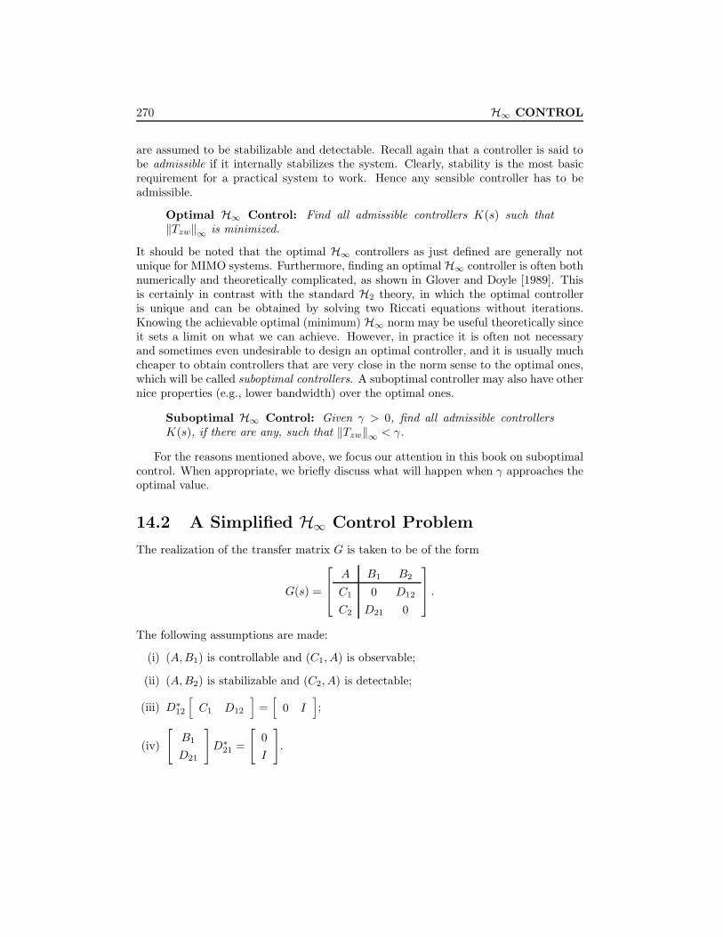
270 H∞ CONTROL
are assumed to be stabilizable and detectable. Recall again that a controller is said tobe admissible if it internally stabilizes the system. Clearly, stability is the most basicrequirement for a practical system to work. Hence any sensible controller has to beadmissible.
Optimal H∞ Control: Find all admissible controllers K(s) such that‖Tzw‖∞ is minimized.
It should be noted that the optimal H∞ controllers as just defined are generally notunique for MIMO systems. Furthermore, finding an optimal H∞ controller is often bothnumerically and theoretically complicated, as shown in Glover and Doyle [1989]. Thisis certainly in contrast with the standard H2 theory, in which the optimal controlleris unique and can be obtained by solving two Riccati equations without iterations.Knowing the achievable optimal (minimum) H∞ norm may be useful theoretically sinceit sets a limit on what we can achieve. However, in practice it is often not necessaryand sometimes even undesirable to design an optimal controller, and it is usually muchcheaper to obtain controllers that are very close in the norm sense to the optimal ones,which will be called suboptimal controllers. A suboptimal controller may also have othernice properties (e.g., lower bandwidth) over the optimal ones.
Suboptimal H∞ Control: Given γ > 0, find all admissible controllersK(s), if there are any, such that ‖Tzw‖∞ < γ.
For the reasons mentioned above, we focus our attention in this book on suboptimalcontrol. When appropriate, we briefly discuss what will happen when γ approaches theoptimal value.
14.2 A Simplified H∞ Control Problem
The realization of the transfer matrix G is taken to be of the form
G(s) =
A B1 B2
C1 0 D12
C2 D21 0
.The following assumptions are made:
(i) (A,B1) is controllable and (C1, A) is observable;
(ii) (A,B2) is stabilizable and (C2, A) is detectable;
(iii) D∗12
[C1 D12
]=[
0 I];
(iv)
[B1
D21
]D∗21 =
[0I
].

14.2. A Simplified H∞ Control Problem 271
Two additional assumptions that are implicit in the assumed realization for G(s) arethat D11 = 0 and D22 = 0. As we mentioned in the last chapter, D22 6= 0 does not poseany problem since it is easy to form an equivalent problem with D22 = 0 by a linearfractional transformation on the controller K(s). However, relaxing the assumptionD11 = 0 complicates the formulas substantially.
The H∞ solution involves the following two Hamiltonian matrices:
H∞ :=
[A γ−2B1B
∗1 −B2B
∗2
−C∗1C1 −A∗
], J∞ :=
[A∗ γ−2C∗1C1 − C∗2C2
−B1B∗1 −A
].
The important difference here from the H2 problem is that the (1,2)-blocks are not signdefinite, so we cannot use Theorem 12.4 in Chapter 12 to guarantee that H∞ ∈ dom(Ric)or Ric(H∞) ≥ 0. Indeed, these conditions are intimately related to the existence ofH∞ suboptimal controllers. Note that the (1,2)-blocks are a suggestive combination ofexpressions from the H∞ norm characterization in Chapter 4 (or bounded real lemmain Chapter 12) and from the H2 synthesis of Chapter 13. It is also clear that if γapproaches infinity, then these two Hamiltonian matrices become the corresponding H2
control Hamiltonian matrices. The reasons for the form of these expressions shouldbecome clear through the discussions and proofs for the following theorem.
Theorem 14.1 There exists an admissible controller such that ‖Tzw‖∞ < γ iff thefollowing three conditions hold:
(i) H∞ ∈ dom(Ric) and X∞ := Ric(H∞) > 0;
(ii) J∞ ∈ dom(Ric) and Y∞ := Ric(J∞) > 0;
(iii) ρ(X∞Y∞) < γ2 .
Moreover, when these conditions hold, one such controller is
Ksub(s) :=
[A∞ −Z∞L∞F∞ 0
]where
A∞ := A+ γ−2B1B∗1X∞ +B2F∞ + Z∞L∞C2
F∞ := −B∗2X∞, L∞ := −Y∞C∗2 , Z∞ := (I − γ−2Y∞X∞)−1.
Furthermore, the set of all admissible controllers such that ‖Tzw‖∞ < γ equals the setof all transfer matrices from y to u in
M∞
Q
u y
-
M∞(s) =
A∞ −Z∞L∞ Z∞B2
F∞ 0 I
−C2 I 0
where Q ∈ RH∞, ‖Q‖∞ < γ.

272 H∞ CONTROL
We shall only give a proof of the first part of the theorem; the proof for the all-controller parameterization needs much more work and is omitted (see Zhou, Doyle,and Glover [1996] for a comprehensive treatment of the related topics). We shall firstshow some preliminary results.
Lemma 14.2 Suppose that X ∈ Rn×n, Y ∈ Rn×n, with X = X∗ > 0, and Y = Y ∗ > 0.Let r be a positive integer. Then there exist matrices X12 ∈ Rn×r, X2 ∈ Rr×r such thatX2 = X∗2 [
X X12
X∗12 X2
]> 0 and
[X X12
X∗12 X2
]−1
=
[Y ?
? ?
]
if and only if [X In
In Y
]≥ 0 and rank
[X In
In Y
]≤ n+ r.
Proof. (⇐) By the assumption, there is a matrix X12 ∈ Rn×r such that X − Y −1 =X12X
∗12. Defining X2 := Ir completes the construction.
(⇒) Using Schur complements,
Y = X−1 +X−1X12(X2 −X∗12X−1X12)−1X∗12X
−1.
Inverting, using the matrix inversion lemma, gives
Y −1 = X −X12X−12 X∗12.
Hence, X−Y −1 = X12X−12 X∗12 ≥ 0, and, indeed, rank(X−Y −1) =rank(X12X
−12 X∗12) ≤
r. 2
Lemma 14.3 There exists an rth-order admissible controller such that ‖Tzw‖∞ < γonly if the following three conditions hold:
(i) There exists a Y1 > 0 such that
AY1 + Y1A∗ + Y1C
∗1C1Y1/γ
2 +B1B∗1 − γ2B2B
∗2 < 0. (14.1)
(ii) There exists an X1 > 0 such that
X1A+A∗X1 +X1B1B∗1X1/γ
2 + C∗1C1 − γ2C∗2C2 < 0. (14.2)
(iii)
[X1/γ In
In Y1/γ
]≥ 0 rank
[X1/γ In
In Y1/γ
]≤ n+ r.

14.2. A Simplified H∞ Control Problem 273
Proof. Suppose that there exists an rth-order controller K(s) such that ‖Tzw‖∞ < γ.Let K(s) have a state-space realization
K(s) =
[A B
C D
].
Then
Tzw = F`(G,K) =
A+B2DC2 B2C B1 +B2DD21
BC2 A BD21
C1 +D12DC2 D12C D12DD21
=:
[Ac Bc
Cc Dc
].
DenoteR = γ2I −D∗cDc, R = γ2I −DcD
∗c .
By Corollary 12.3, there exists an X =
[X1 X12
X∗12 X2
]> 0 such that
X(Ac+BcR−1D∗cCc)+(Ac+BcR
−1D∗cCc)∗X+XBcR
−1B∗c X+C∗c R−1Cc < 0. (14.3)
This gives, after much algebraic manipulation,
X1A+A∗X1 +X1B1B∗1X1/γ
2 + C∗1C1 − γ2C∗2C2
+(X1B1D +X12B + γ2C∗2 )(γ2I − D∗D)−1(X1B1D +X12B + γ2C∗2 )∗ < 0,
which implies that
X1A+A∗X1 +X1B1B∗1X1/γ
2 + C∗1C1 − γ2C∗2C2 < 0.
On the other hand, letY = γ2X−1
and partition Y as Y =
[Y1 Y12
Y ∗12 Y2
]> 0. Then
(Ac+BcR−1D∗cCc)Y + Y (Ac+BcR
−1D∗cCc)∗+ Y C∗c R
−1CcY +BcR−1B∗c < 0. (14.4)
This givesAY1 + Y1A
∗ +B1B∗1 − γ2B2B
∗2 + Y1C
∗1C1Y1/γ
2
+(Y1C∗1 D∗ + Y12C
∗ + γ2B2)(γ2I − DD∗)−1(Y1C∗1 D∗ + Y12C
∗ + γ2B2)∗ < 0,
which implies that
AY1 + Y1A∗ +B1B
∗1 − γ2B2B
∗2 + Y1C
∗1C1Y1/γ
2 < 0.

274 H∞ CONTROL
By Lemma 14.2, givenX1 > 0 and Y1 > 0, there existsX12 andX2 such that Y = γ2X−1
or Y /γ = (X/γ)−1: [X1/γ X12/γ
X∗12/γ X2/γ
]−1
=
[Y1/γ ?
? ?
]if and only if [
X1/γ In
In Y1/γ
]≥ 0 rank
[X1/γ In
In Y1/γ
]≤ n+ r.
2
To show that the inequalities in the preceding lemma imply the existence of thestabilizing solutions to the Riccati equations of X∞ and Y∞, we need the followingtheorem.
Theorem 14.4 Let R ≥ 0 and suppose (A,R) is controllable and there is an X = X∗
such thatQ(X) := XA+A∗X +XRX +Q < 0. (14.5)
Then there exists a solution X+ > X to the Riccati equation
X+A+A∗X+ +X+RX+ +Q = 0 (14.6)
such that A+RX+ is antistable.
Proof. Let R = BB∗ for some B. Note the fact that (A,R) is controllable iff (A,B)is. Let X be such that Q(X) < 0. Since (A,B) is controllable, there is an F0 such that
A0 := A−BF0
is antistable. Now let X0 = X∗0 be the unique solution to the Lyapunov equation
X0A0 +A∗0X0 − F ∗0 F0 +Q = 0.
DefineF0 := F0 +B∗X,
and we have the following equation:
(X0 −X)A0 +A∗0(X0 −X) = F ∗0 F0 −Q(X) > 0.
The antistability of A0 implies that
X0 > X.
Starting with X0, we shall define a nonincreasing sequence of Hermitian matrices Xi.Associated with Xi, we shall also define a sequence of antistable matrices Ai and a

14.2. A Simplified H∞ Control Problem 275
sequence of matrices Fi. Assume inductively that we have already defined matricesXi, Ai, and Fi for i up to n− 1 such that Xi is Hermitian and
X0 ≥ X1 ≥ · · · ≥ Xn−1 > X,
Ai = A−BFi is antistable, i = 0, . . . , n− 1;
Fi = −B∗Xi−1, i = 1, . . . , n− 1;
XiAi +A∗iXi = F ∗i Fi −Q, i = 0, 1, . . . , n− 1. (14.7)
Next, introduceFn = −B∗Xn−1,
An = A−BFn.First we show that An is antistable. Using equation (14.7), with i = n− 1, we get
Xn−1An +A∗nXn−1 +Q− F ∗nFn − (Fn − Fn−1)∗(Fn − Fn−1) = 0. (14.8)
LetFn := Fn +B∗X ;
then
(Xn−1−X)An+A∗n(Xn−1−X) = −Q(X)+F ∗nFn+(Fn−Fn−1)∗(Fn−Fn−1) > 0, (14.9)
which implies that An is antistable by Lyapunov theorem since Xn−1 −X > 0.Now we introduce Xn as the unique solution of the Lyapunov equation:
XnAn +A∗nXn = F ∗nFn −Q. (14.10)
Then Xn is Hermitian. Next, we have
(Xn −X)An +A∗n(Xn −X) = −Q(X) + F ∗n Fn > 0,
and, by using equation (14.8),
(Xn−1 −Xn)An +A∗n(Xn−1 −Xn) = (Fn − Fn−1)∗(Fn − Fn−1) ≥ 0.
Since An is antistable, we have
Xn−1 ≥ Xn > X.
We have a nonincreasing sequence Xi, and the sequence is bounded below by Xi > X .Hence the limit
X+ := limn→∞
Xn
exists and is Hermitian, and we have X+ ≥ X . Passing the limit n → ∞ in equation(14.10), we get Q(X+) = 0. So X+ is a solution of equation (14.6).
Note that X+ −X ≥ 0 and
(X+ −X)A+ +A∗+(X+ −X) = −Q(X) + (X+ −X)R(X+ −X) > 0. (14.11)
Hence, X+ −X > 0 and A+ = A+RX+ is antistable. 2

276 H∞ CONTROL
Lemma 14.5 There exists an admissible controller such that ‖Tzw‖∞ < γ only if thefollowing three conditions hold:
(i) There exists a stabilizing solution X∞ > 0 to
X∞A+A∗X∞ +X∞(B1B∗1/γ
2 −B2B∗2)X∞ + C∗1C1 = 0. (14.12)
(ii) There exists a stabilizing solution Y∞ > 0 to
AY∞ + Y∞A∗ + Y∞(C∗1C1/γ
2 − C∗2C2)Y∞ +B1B∗1 = 0. (14.13)
(iii)
[γY −1∞ In
In γX−1∞
]> 0 or ρ(X∞Y∞) < γ2.
Proof. Applying Theorem 14.4 to part (i) of Lemma 14.3, we conclude that thereexists a Y > Y1 > 0 such that
AY + Y A∗ + Y C∗1C1Y/γ2 +B1B
∗1 − γ2B2B
∗2 = 0
and A+ C∗1C1Y/γ2 is antistable. Let X∞ := γ2Y −1; we have
X∞A+A∗X∞ +X∞(B1B∗1/γ
2 −B2B∗2 )X∞ + C∗1C1 = 0 (14.14)
and
A+ (B1B∗1/γ
2−B2B∗2)X∞ = −X−1
∞ (A+C∗1C1X−1∞ )X∞ = −X−1
∞ (A+C∗1C1Y/γ2)X∞
is stable.Similarly, applying Theorem 14.4 to part (ii) of Lemma 14.3, we conclude that there
exists an X > X1 > 0 such that
XA+A∗X +XB1B∗1X/γ
2 + C∗1C1 − γ2C∗2C2 = 0
and A+B1B∗1X/γ
2 is antistable. Let Y∞ := γ2X−1, we have
AY∞ + Y∞A∗ + Y∞(C∗1C1/γ
2 − C∗2C2)Y∞ +B1B∗1 = 0 (14.15)
and A+ (C∗1C1/γ2 − C∗2C2)Y∞ is stable.
Finally, note that the rank condition in part (iii) of Lemma 14.3 is automaticallysatisfied by r ≥ n, and[
γY −1∞ In
In γX−1∞
]=
[X/γ In
In Y/γ
]>
[X1/γ In
In Y1/γ
]≥ 0
or ρ(X∞Y∞) < γ2. 2

14.2. A Simplified H∞ Control Problem 277
Proof of Theorem 14.1: To complete the proof, we only need to show that thecontroller Ksub given in Theorem 14.1 renders ‖Tzw‖∞ < γ. Note that the closed-looptransfer function with Ksub is given by
Tzw =
A B2F∞ B1
−Z∞L∞C2 A∞ −Z∞L∞D21
C1 D12F∞ 0
=:
[Ac Bc
Cc Dc
].
Define
P =
[γ2Y −1
∞ −γ2Y −1∞ Z−1
∞−γ2(Z∗∞)−1Y −1
∞ γ2Y −1∞ Z−1
∞
].
Then it is easy to show that P > 0 and
PAc +A∗cP + PBcB∗cP/γ
2 + C∗cCc = 0.
Moreover,
Ac +BcB∗cP/γ
2 =
[A+B1B
∗1Y−1∞ B2F∞ −B1B
∗1Y−1∞ Z−1
∞0 A+B1B
∗1X∞/γ
2 +B2F∞
]
has no eigenvalues on the imaginary axis since A+B1B∗1X∞/γ
2 +B2F∞ is stable andA+B1B
∗1Y−1∞ is antistable. Thus, by Corollary 12.3, ‖Tzw‖∞ < γ. 2
Remark 14.1 It is appropriate to point out that the conditions stated in Lemma 14.3are, in fact, necessary and sufficient; see Gahinet and Apkarian [1994] and Gahinet[1996] for a linear matrix inequality (LMI) approach to the H∞ problem. But thenecessity should be suitably interpreted. For example, if one finds an X1 > 0 and aY1 > 0 satisfying conditions (i) and (ii) but not condition (iii), this does not imply thatthere is no admissible H∞ controller since there might be other X1 > 0 and Y1 > 0 thatsatisfy all three conditions. For example, consider γ = 1 and
G(s) =
−1
[1 0
]1[
10
]0
[01
]1
[0 1
]0
.
It is easy to check that X1 = Y1 = 0.5 satisfy (i) and (ii) but not (iii). Nevertheless,we shall show in the next section that γopt = 0.7321 and thus a suboptimal controllerexists for γ = 1. In fact, we can check that 1 < X1 < 2, 1 < Y1 < 2 also satisfy (i), (ii)and (iii). 3

278 H∞ CONTROL
Example 14.1 Consider the feedback system shown in Figure 6.3 with
P =50(s+ 1.4)
(s+ 1)(s+ 2), We =
2s+ 0.2
, Wu =s+ 1s+ 10
.
We shall design a controller so that the H∞ norm from w =
[d
di
]to z =
[e
u
]is
minimized. Note that[e
u
]=
[We(I + PK)−1 We(I + PK)−1P
−WuK(I + PK)−1 −WuK(I + PK)−1P
][d
di
]=: Tzw
[d
di
].
Then the problem can be set up in an LFT framework with
G(s) =
We WeP −WeP
0 0 −Wu
I P −P
=
−0.2 2 2 0 2 0 00 −1 0 0 0 20 −200 0 −2 0 0 30 −300 0 0 −10 0 0 −3
1 0 0 0 0 0 00 0 0 −3 0 0 −10 1 1 0 1 0 0
.
A suboptimal H∞ controller can be computed by using the following command:
[K,Tzw, γsubopt] = hinfsyn(G,ny,nu, γmin, γmax, tol)
where ny and nu are the dimensions of y and u; γmin and γmax are, respectively a lowerbound and an upper bound for γopt; and tol is a tolerance to the optimal value. Setny = 1, nu = 1, γmin = 0, γmax = 10, tol = 0.0001; we get γsubopt = 0.7849 and asuboptimal controller
K =12.82(s/10 + 1)(s/7.27 + 1)(s/1.4 + 1)
(s/32449447.67 + 1)(s/22.19 + 1)(s/1.4 + 1)(s/0.2 + 1).
If we set tol = 0.01, we would get γsubopt = 0.7875 and a suboptimal controller
K =12.78(s/10 + 1)(s/7.27 + 1)(s/1.4 + 1)
(s/2335.59 + 1)(s/21.97 + 1)(s/1.4 + 1)(s/0.2 + 1).
The only significant difference between K and K is the exact location of the far-awaystable controller pole. Figure 14.1 shows the closed-loop frequency response of σ (Tzw)and Figure 14.2 shows the frequency responses of S, T,KS, and SP .

14.2. A Simplified H∞ Control Problem 279
10−2
10−1
100
101
102
103
104
10−1
100
frequency (rad/sec)
Figure 14.1: The closed-loop frequency responses of σ(Tzw) withK (solid line) and K (dashed line)
10−2
10−1
100
101
102
103
104
10−3
10−2
10−1
100
101
S
T
KS
SP
frequency (rad/sec)
Figure 14.2: The frequency responses of S, T,KS, and SP with K

280 H∞ CONTROL
Example 14.2 Consider again the two-mass/spring/damper system shown in Figure 4.2.Assume that F1 is the control force, F2 is the disturbance force, and the measurementsof x1 and x2 are corrupted by measurement noise:
y =
[y1
y2
]=
[x1
x2
]+Wn
[n1
n2
], Wn =
0.01(s+ 10)s+ 100
0
00.01(s+ 10)s+ 100
.Our objective is to design a control law so that the effect of the disturbance force F2 onthe positions of the two masses, x1 and x2, are reduced in a frequency range 0 ≤ ω ≤ 2.
The problem can be set up as shown in Figure 14.3, where We =
[W1 00 W2
]is the
performance weight and Wu is the control weight. In order to limit the control force,we shall choose
Wu =s+ 5s+ 50
.
eK Plant We
Wn
Wu
- -
?
-
6
6
?-
u = F1
w1 = F2
z2
z1
[x1
x2
]
w2 =
[n1
n2
]y
Figure 14.3: Rejecting the disturbance force F2 by a feedback control
Now let u = F1, w =
F2
n1
n2
; then the problem can be formulated in an LFT form
with
G(s) =
[WeP1 0
0 0
] [WeP2
Wu
][P1 Wn
]P2

14.2. A Simplified H∞ Control Problem 281
where P1 and P2 denote the transfer matrices from F1 and F2 to
[x1
x2
], respectively.
LetW1 =
5s/2 + 1
, W2 = 0.
That is, we only want to reject the effect of the disturbance force F2 on the position x1.Then the optimal H2 performance is ‖F`(G,K2)‖2 = 2.6584 and the H∞ performancewith the optimal H2 controller is ‖F`(G,K2)‖∞ = 2.6079 while the optimal H∞ perfor-mance with an H∞ controller is ‖F`(G,K∞)‖∞ = 1.6101. This means that the effectof the disturbance force F2 in the desired frequency rang 0 ≤ ω ≤ 2 will be effectivelyreduced with the H∞ controller K∞ by 5/1.6101 = 3.1054 times at x1. On the otherhand, let
W1 = 0, W2 =5
s/2 + 1.
That is, we only want to reject the effect of the disturbance force F2 on the position x2.Then the optimal H2 performance is ‖F`(G,K2)‖2 = 0.1659 and the H∞ performancewith the optimal H2 controller is ‖F`(G,K2)‖∞ = 0.5202 while the optimal H∞ perfor-mance with an H∞ controller is ‖F`(G,K∞)‖∞ = 0.5189. This means that the effectof the disturbance force F2 in the desired frequency rang 0 ≤ ω ≤ 2 will be effectivelyreduced with the H∞ controller K∞ by 5/0.5189 = 9.6358 times at x2.
10−1
100
101
10−1
100
101
H∞ Control
H2 Control
frequency (rad/sec)
The
larg
est s
ingula
r valu
e
Figure 14.4: The largest singular value plot of the closed-loop system Tzw with an H2
controller and an H∞ controller
Finally, set
W1 = W2 =5
s/2 + 1.

282 H∞ CONTROL
That is, we want to reject the effect of the disturbance force F2 on both x1 and x2. Thenthe optimal H2 performance is ‖F`(G,K2)‖2 = 4.087 and the H∞ performance withthe optimal H2 controller is ‖F`(G,K2)‖∞ = 6.0921 while the optimal H∞ performancewith an H∞ controller is ‖F`(G,K∞)‖∞ = 4.3611. This means that the effect of thedisturbance force F2 in the desired frequency rang 0 ≤ ω ≤ 2 will only be effectivelyreduced with the H∞ controller K∞ by 5/4.3611 = 1.1465 times at both x1 and x2.This result shows clearly that it is very hard to reject the disturbance effect on bothpositions at the same time. The largest singular value Bode plots of the closed-loopsystem are shown in Figure 14.4. We note that the H∞ controller typically gives arelatively flat frequency response since it tries to minimize the peak of the frequencyresponse. On the other hand, the H2 controller would typically produce a frequencyresponse that rolls off fast in the high-frequency range but with a large peak in thelow-frequency range.
14.3 Optimality and Limiting Behavior
In this section, we will discuss, without proof, the behavior of the H∞ suboptimalsolution as γ varies, especially as γ approaches the infima achievable norm, denoted byγopt. Since Theorem 14.1 gives necessary and sufficient conditions for the existence ofan admissible controller such that ‖Tzw‖∞ < γ, γopt is the infimum over all γ such thatconditions (i)–(iii) are satisfied. Theorem 14.1 does not give an explicit formula for γopt,but, just as for the H∞ norm calculation, it can be computed as closely as desired by asearch technique.
Although we have not focused on the problem of H∞ optimal controllers, the as-sumptions in this book make them relatively easy to obtain in most cases. In addition todescribing the qualitative behavior of suboptimal solutions as γ varies, we will indicatewhy the descriptor version of the controller formulas below can usually provide formulasfor the optimal controller when γ = γopt.
As γ → ∞, H∞ → H2, X∞ → X2, etc., and Ksub → K2. This fact is the result ofthe particular choice of the suboptimal controller. While it could be argued that Ksub
is a natural choice, this connection with H2 actually hints at deeper interpretations. Infact, Ksub is the minimum entropy solution (see Section 14.4) as well as the minimaxcontroller for ‖z‖22 − γ2‖w‖22.
If γ2 ≥ γ1 > γopt, then X∞(γ1) ≥ X∞(γ2) and Y∞(γ1) ≥ Y∞(γ2). Thus X∞ andY∞ are decreasing functions of γ, as is ρ(X∞Y∞). At γ = γopt, any one of the threeconditions in Theorem 14.1 can fail. If only condition (iii) fails, then it is relativelystraightforward to show that the descriptor formulas below for γ = γopt are optimal;that is, the optimal controller is given by
(I − γ−2optY∞X∞) ˙x = Asx− L∞y (14.16)
u = F∞x (14.17)

14.3. Optimality and Limiting Behavior 283
where As := A+B2F∞ + L∞C2 + γ−2optY∞A
∗X∞ + γ−2optB1B
∗1X∞ + γ−2
optY∞C∗1C1. (See
Example 14.3.)
The formulas in Theorem 14.1 are not well-defined in the optimal case because theterm (I − γ−2
optX∞Y∞) is not invertible. It is possible but far less likely that conditions(i) or (ii) would fail before (iii). To see this, consider (i) and let γ1 be the largest γfor which H∞ fails to be in dom(Ric) because the H∞ matrix fails to have either thestability property or the complementarity property. The same remarks will apply to (ii)by duality.
If complementarity fails at γ = γ1, then ρ(X∞) → ∞ as γ → γ1. For γ < γ1,H∞ may again be in dom(Ric), but X∞ will be indefinite. For such γ, the controlleru = −B∗2X∞x would make ‖Tzw‖∞ < γ but would not be stabilizing. (See part 1of Example 14.3.) If the stability property fails at γ = γ1, then H∞ 6∈ dom(Ric)but Ric can be extended to obtain X∞ so that a controller can be obtained to make‖Tzw‖∞ = γ1. The stability property will also not hold for any γ ≤ γ1, and no controllerwhatsoever exists that makes ‖Tzw‖∞ < γ1. In other words, if stability breaks downfirst, then the infimum over stabilizing controllers equals the infimum over all controllers,stabilizing or otherwise. (See part 2 of Example 14.3.) In view of this, we would typicallyexpect that complementarity would fail first.
Complementarity failing at γ = γ1 means ρ(X∞)→∞ as γ → γ1, so condition (iii)would fail at even larger values of γ, unless the eigenvectors associated with ρ(X∞) asγ → γ1 are in the null space of Y∞. Thus condition (iii) is the most likely of all to failfirst. If condition (i) or (ii) fails first because the stability property fails, the formulasin Theorem 14.1 as well as their descriptor versions are optimal at γ = γopt. This isillustrated in Example 14.3. If the complementarity condition fails first, [but (iii) doesnot fail], then obtaining formulas for the optimal controllers is a more subtle problem.
Example 14.3 Let an interconnected dynamical system realization be given by
G(s) =
a
[1 0
]1[
10
]0
[01
]1
[0 1
]0
.
Then all assumptions for output feedback problem are satisfied and
H∞ =
[a 1−γ2
γ2
−1 −a
], J∞ =
[a 1−γ2
γ2
−1 −a
].
The eigenvalues of H∞ and J∞ are given by±√
(a2 + 1)γ2 − 1γ
.

284 H∞ CONTROL
If γ >1√
a2 + 1, then X−(H∞) and X−(J∞) exist and
X−(H∞) = Im
[ √(a2+1)γ2−1−aγ
γ
1
]
X−(J∞) = Im
[ √(a2+1)γ2−1−aγ
γ
1
].
We shall consider two cases:
1) a > 0: In this case, the complementary property of dom(Ric) will fail before thestability property fails since√
(a2 + 1)γ2 − 1− aγ = 0
when γ = 1.
Nevertheless, if γ >1√
a2 + 1and γ 6= 1, then H∞ ∈ dom(Ric) and
X∞ =γ√
(a2 + 1)γ2 − 1− aγ=
> 0; if γ > 1< 0; if 1√
a2+1< γ < 1.
Note that if γ > 1, then H∞ ∈ dom(Ric), J∞ ∈ dom(Ric), and
X∞ =γ√
(a2 + 1)γ2 − 1− aγ> 0
Y∞ =γ√
(a2 + 1)γ2 − 1− aγ> 0.
Hence conditions (i) and (ii) in Theorem 14.1 are satisfied, and we need to checkcondition (iii). Since
ρ(X∞Y∞) =γ2
(√
(a2 + 1)γ2 − 1− aγ)2,
it is clear that ρ(X∞Y∞) → ∞ when γ → 1. So condition (iii) will fail beforecondition (i) or (ii) fails.
2) a < 0: In this case, the complementary property is always satisfied, and, further-more, H∞ ∈ dom(Ric), J∞ ∈ dom(Ric), and
X∞ =γ√
(a2 + 1)γ2 − 1− aγ> 0

14.3. Optimality and Limiting Behavior 285
Y∞ =γ√
(a2 + 1)γ2 − 1− aγ> 0
for γ >1√
a2 + 1.
However, for γ ≤ 1√a2 + 1
, H∞ 6∈ dom(Ric) since stability property fails. Nev-
ertheless, in this case, if γ0 =1√
a2 + 1, we can extend the dom(Ric) to include
those matrices H∞ with imaginary axis eigenvalues as
X−(H∞) = Im
[−a1
]
such that X∞ = −1a
is a solution to the Riccati equation
A∗X∞ +X∞A+ C∗1C1 + γ−20 X∞B1B
∗1X∞ −X∞B2B
∗2X∞ = 0
and A+ γ−20 B1B
∗1X∞ −B2B
∗2X∞ = 0. It can be shown that
ρ(X∞Y∞) =γ2
(√
(a2 + 1)γ2 − 1− aγ)2< γ2
is satisfied if and only if
γ >√a2 + 2 + a
(>
1√a2 + 1
).
So condition (iii) of Theorem 14.1 will fail before either (i) or (ii) fails.
In both a > 0 and a < 0 cases, the optimal γ for the output feedback is given by
γopt =√a2 + 2 + a
and the optimal controller given by the descriptor formula in equations (14.16) and (14.17)is a constant. In fact,
uopt = − γopt√(a2 + 1)γ2
opt − 1− aγopt
y.
For instance, let a = −1 then γopt =√
3− 1 = 0.7321 and uopt = −0.7321 y. Further,
Tzw =
−1.7321 1 −0.7321
1 0 0−0.7321 0 −0.7321
.It is easy to check that ‖Tzw‖∞ = 0.7321.

286 H∞ CONTROL
14.4 Minimum Entropy Controller
Let T be a transfer matrix with ‖T‖∞ < γ. Then the entropy of T (s) is defined by
I(T, γ) = − γ2
2π
∫ ∞−∞
ln∣∣det
(I − γ−2T ∗(jω)T (jω)
)∣∣ dω.It is easy to see that
I(T, γ) = − γ2
2π
∫ ∞−∞
∑i
ln∣∣1− γ−2σ2
i (T (jω))∣∣ dω
and I(T, γ) ≥ 0, where σi (T (jω)) is the ith singular value of T (jω). It is also easy toshow that
limγ→∞
I(T, γ) =1
2π
∫ ∞−∞
∑i
σ2i (T (jω))dω = ‖T‖22 .
Thus the entropy I(T, γ) is, in fact , a performance index measuring the tradeoff betweenthe H∞ optimality (γ → ‖T‖∞) and the H2 optimality (γ →∞).
It has been shown in Glover and Mustafa [1989] that the suboptimal controller givenin Theorem 14.1 is actually the controller that satisfies the norm condition ‖Tzw‖∞ < γand minimizes the following entropy:
− γ2
2π
∫ ∞−∞
ln∣∣det
(I − γ−2T ∗zw(jω)Tzw(jω)
)∣∣ dω.Therefore, the given suboptimal controller is also called the minimum entropy controller[maximum entropy controller if the entropy is defined as I(T, γ) = −I(T, γ)].
Related MATLAB Commands: hinfsyne, hinffi
14.5 An Optimal Controller
To offer a general idea about the appearance of an optimal controller, we shall give inthe following (without proof) the conditions under which an optimal controller existsand an explicit formula for an optimal controller.
Theorem 14.6 There exists an admissible controller such that ‖Tzw‖∞ ≤ γ iff thefollowing three conditions hold:
(i) There exists a full column rank matrix[X∞1
X∞2
]∈ R2n×n

14.5. An Optimal Controller 287
such that
H∞
[X∞1
X∞2
]=
[X∞1
X∞2
]TX , Re λi(TX) ≤ 0 ∀i
andX∗∞1X∞2 = X∗∞2X∞1;
(ii) There exists a full column rank matrix[Y∞1
Y∞2
]∈ R2n×n
such that
J∞
[Y∞1
Y∞2
]=
[Y∞1
Y∞2
]TY , Re λi(TY ) ≤ 0 ∀i
andY ∗∞1Y∞2 = Y ∗∞2Y∞1;
(iii) [X∗∞2X∞1 γ−1X∗∞2Y∞2
γ−1Y ∗∞2X∞2 Y ∗∞2Y∞1
]≥ 0.
Moreover, when these conditions hold, one such controller is
Kopt(s) := CK(sEK −AK)+BK
where
EK := Y ∗∞1X∞1 − γ−2Y ∗∞2X∞2
BK := Y ∗∞2C∗2
CK := −B∗2X∞2
AK := EKTX −BKC2X∞1 = T ∗YEK + Y ∗∞1B2CK .
Remark 14.2 It is simple to show that if X∞1 and Y∞1 are nonsingular and ifX∞ = X∞2X
−1∞1 and Y∞ = Y∞2Y
−1∞1 , then condition (iii) in the preceding theorem
is equivalent to X∞ ≥ 0, Y∞ ≥ 0, and ρ(Y∞X∞) ≤ γ2. So, in this case, the conditionsfor the existence of an optimal controller can be obtained from “taking the limit” ofthe corresponding conditions in Theorem 14.1. Moreover, the controller given above isreduced to the descriptor form given in equations (14.16) and (14.17). 3

288 H∞ CONTROL
14.6 General H∞ Solutions
Consider the system described by the block diagram
G
K
z
y
w
u
-
where, as usual, G and K are assumed to be real rational and proper with K constrainedto provide internal stability. The controller is said to be admissible if it is real rational,proper, and stabilizing. Although we are taking everything to be real, the resultspresented here are still true for the complex case with some obvious modifications. Wewill again only be interested in characterizing all suboptimal H∞ controllers.
The realization of the transfer matrix G is taken to be of the form
G(s) =
A B1 B2
C1 D11 D12
C2 D21 0
=
[A B
C D
],
which is compatible with the dimensions of z(t) ∈ Rp1 , y(t) ∈ Rp2 , w(t) ∈ Rm1 ,u(t) ∈ Rm2 , and the state x(t) ∈ Rn. The following assumptions are made:
(A1) (A,B2) is stabilizable and (C2, A) is detectable;
(A2) D12 =
[0I
]and D21 =
[0 I
];
(A3)
[A− jωI B2
C1 D12
]has full column rank for all ω;
(A4)
[A− jωI B1
C2 D21
]has full row rank for all ω.
Assumption (A1) is necessary for the existence of stabilizing controllers. The as-sumptions in (A2) mean that the penalty on z = C1x + D12u includes a nonsingular,normalized penalty on the control u, that the exogenous signal w includes both plantdisturbance and sensor noise, and that the sensor noise weighting is normalized andnonsingular. Relaxation of (A2) leads to singular control problems; see Stroorvogel[1992]. For those problems that have D12 full column rank and D21 full row rank butdo not satisfy assumption (A2), a normalizing procedure is given in the next section sothat an equivalent new system will satisfy this assumption.

14.6. General H∞ Solutions 289
Assumptions (A3) and (A4) are made for a technical reason: Together with (A1)they guarantee that the two Hamiltonian matrices in the corresponding H2 problembelong to dom(Ric), as we have seen in Chapter 13. Dropping (A3) and (A4) wouldmake the solution very complicated. A further discussion of the assumptions and theirpossible relaxation will be provided in Section 14.7.
The main result is now stated in terms of the solutions of the X∞ and Y∞ Riccatiequations together with the “state feedback” and “output injection” matrices F and L.
R := D∗1•D1• −[γ2Im1 0
0 0
], where D1• := [D11 D12]
R := D•1D∗•1 −
[γ2Ip1 0
0 0
], where D•1 :=
[D11
D21
]
H∞ :=
[A 0
−C∗1C1 −A∗
]−[
B
−C∗1D1•
]R−1
[D∗1•C1 B∗
]J∞ :=
[A∗ 0
−B1B∗1 −A
]−[
C∗
−B1D∗•1
]R−1
[D•1B∗1 C
]X∞ := Ric(H∞) Y∞ := Ric(J∞)
F :=
[F1∞
F2∞
]:= −R−1 [D∗1•C1 +B∗X∞]
L :=[L1∞ L2∞
]:= −[B1D
∗•1 + Y∞C
∗]R−1
Partition D, F1∞, and L1∞ are as follows:
[F ′
L′ D
]=
F ∗11∞ F ∗12∞ F ∗2∞
L∗11∞ D1111 D1112 0L∗12∞ D1121 D1122 I
L∗2∞ 0 I 0
.Remark 14.3 In the above matrix partitioning, some matrices may not exist depend-ing on whether D12 or D21 is square. This issue will be discussed further later. For thetime being, we shall assume that all matrices in the partition exist. 3
Theorem 14.7 Suppose G satisfies the assumptions (A1)–(A4).
(a) There exists an admissible controller K(s) such that ||F`(G,K)||∞ < γ (i.e.,‖Tzw‖∞ < γ) if and only if

290 H∞ CONTROL
(i) γ > max(σ[D1111, D1112, ], σ[D∗1111, D∗1121]);
(ii) H∞ ∈ dom(Ric) with X∞ = Ric(H∞) ≥ 0;
(iii) J∞ ∈ dom(Ric) with Y∞ = Ric(J∞) ≥ 0;
(iv) ρ(X∞Y∞) < γ2.
(b) Given that the conditions of part (a) are satisfied, then all rational internallystabilizing controllers K(s) satisfying ||F`(G,K)||∞ < γ are given by
K = F`(M∞, Q) for arbitrary Q ∈ RH∞ such that ‖Q‖∞ < γ
where
M∞ =
A B1 B2
C1 D11 D12
C2 D21 0
D11 = −D1121D
∗1111(γ2I −D1111D
∗1111)−1D1112 −D1122
D12 ∈ Rm2×m2 and D21 ∈ Rp2×p2 are any matrices (e.g., Cholesky factors) satisfying
D12D∗12 = I −D1121(γ2I −D∗1111D1111)−1D∗1121,
D∗21D21 = I −D∗1112(γ2I −D1111D∗1111)−1D1112,
and
B2 = Z∞(B2 + L12∞)D12,
C2 = −D21(C2 + F12∞),B1 = −Z∞L2∞ + B2D
−112 D11,
C1 = F2∞ + D11D−121 C2,
A = A+BF + B1D−121 C2
whereZ∞ = (I − γ−2Y∞X∞)−1.
(Note that if D11 = 0 then the formulas are considerably simplified.)
Some Special Cases:
Case 1: D12 = I
In this case
1. In part (a), (i) becomes γ > σ(D1121).

14.7. Relaxing Assumptions 291
2. In part (b)
D11 = −D1122
D12D∗12 = I − γ−2D1121D
∗1121
D∗21D21 = I.
Case 2: D21 = I
In this case
1. In part (a), (i) becomes γ > σ(D1112).
2. In part (b)
D11 = −D1122
D12D∗12 = I
D∗21D21 = I − γ−2D∗1112D1112.
Case 3: D12 = I & D21 = I
In this case
1. In part (a), (i) drops out.
2. In part (b)
D11 = −D1122
D12D∗12 = I
D∗21D21 = I.
14.7 Relaxing Assumptions
In this section, we indicate how the results of Section 14.6 can be extended to moregeneral cases. Let a given problem have the following diagram, where zp(t) ∈ Rp1 ,yp(t) ∈ Rp2 , wp(t) ∈ Rm1 , and up(t) ∈ Rm2 :
P
Kp
zp
yp
wp
up
-

292 H∞ CONTROL
The plant P has the following state-space realization with Dp12 full column rank andDp21 full row rank:
P (s) =
Ap Bp1 Bp2
Cp1 Dp11 Dp12
Cp2 Dp21 Dp22
.The objective is to find all rational proper controllers Kp(s) that stabilize P and||F`(P,Kp)||∞ < γ. To solve this problem, we first transform it to the standard onetreated in the last section. Note that the following procedure can also be applied to theH2 problem (except the procedure for the case D11 6= 0).
Normalize D12 and D21
Perform singular value decompositions to obtain the matrix factorizations
Dp12 = Up
[0I
]Rp, Dp21 = Rp
[0 I
]Up
such that Up and Up are square and unitary and Rp and Rp are square and invertible.Now let
zp = Upz, wp = U∗pw, yp = Rpy, up = R−1p u
andK(s) = RpKp(s)Rp
G(s) =
[U∗p 00 R−1
p
]P (s)
[U∗p 00 R−1
p
]
=
Ap Bp1U
∗p Bp2R
−1p
U∗pCp1 U∗pDp11U∗p U∗pDp12R
−1p
R−1p Cp2 R−1
p Dp21U∗p R−1
p Dp22R−1p
=:
A B1 B2
C1 D11 D12
C2 D21 D22
=
[A B
C D
].
Then
D12 =
[0I
]D21 =
[0 I
],
and the new system is as follows:

14.7. Relaxing Assumptions 293
G
K
z
y
w
u
-
Furthermore, ||F`(P,Kp)||α = ||UpF`(G,K)Up||α = ‖F`(G,K)‖α for α = 2 or ∞since Up and Up are unitary. Moreover, Assumptions (A1), (A3), and (A4) remainunaffected.
Remove the Assumption D22 = 0
Suppose K(s) is a controller for G with D22 set to zero. Then the controller for D22 6= 0is K(I +D22K)−1. Hence there is no loss of generality in assuming D22 = 0.
Relax (A3) and (A4)
Suppose that
G =
0 0 1
0 0 11 1 0
which violates both (A3) and (A4) and corresponds to the robust stabilization of anintegrator. If the controller u = −εx, where ε > 0 is used, then
Tzw =−εss+ ε
, with ‖Tzw‖∞ = ε.
Hence the norm can be made arbitrarily small as ε → 0, but ε = 0 is not admissiblesince it is not stabilizing. This may be thought of as a case where the H∞ optimum isnot achieved on the set of admissible controllers. Of course, for this system, H∞ optimalcontrol is a silly problem, although the suboptimal case is not obviously so.
Relax (A1)
If assumption (A1) is violated, then it is obvious that no admissible controllers exist.Suppose (A1) is relaxed to allow unstabilizable and/or undetectable modes on the jωaxis and internal stability is also relaxed to also allow closed-loop jω axis poles, but(A2)–(A4) is still satisfied. It can be easily shown that under these conditions theclosed-loop H∞ norm cannot be made finite and, in particular, that the unstabilizableand/or undetectable modes on the jω axis must show up as poles in the closed-loopsystem.

294 H∞ CONTROL
Violate (A1) and either or both (A3) and (A4)
Sensible control problems can be posed that violate (A1) and either or both (A3) and(A4). For example, cases when A has modes at s = 0 that are unstabilizable throughB2 and/or undetectable through C2 arise when an integrator is included in a weighton a disturbance input or an error term. In these cases, either (A3) or (A4) are alsoviolated, or the closed-loopH∞ norm cannot be made finite. In many applications, suchproblems can be reformulated so that the integrator occurs inside the loop (essentiallyusing the internal model principle) and is hence detectable and stabilizable. We willshow this process in the next section.
An alternative is to introduce ε perturbations so that (A1), (A3), and (A4) aresatisfied. Roughly speaking, this would produce sensible answers for sensible problems,but the behavior as ε→ 0 could be problematic.
Relax (A2)
In the cases that either D12 is not full column rank or that D21 is not full row rank,improper controllers can give a bounded H∞ norm for Tzw, although the controllerswill not be admissible by our definition. Such singular filtering and control problemshave been well-studied in H2 theory and many of the same techniques go over to theH∞ case (e.g., Willems [1981] and Willems, Kitapci, and Silverman [1986]). A completesolution to the singular problem can be found in Stroorvogel [1992].
14.8 H2 and H∞ Integral Control
It is interesting to note that the H2 and H∞ design frameworks do not, in general,produce integral control. In this section we show how to introduce integral control intothe H2 and H∞ design framework through a simple disturbance rejection problem. Weconsider a feedback system shown in Figure 14.5. We shall assume that the frequencycontents of the disturbance w are effectively modeled by the weighting Wd ∈ RH∞ andthe constraints on control signal are limited by an appropriate choice of Wu ∈ RH∞.In order to let the output y track the reference signal r, we require K to contain anintegrator [i.e., K(s) has a pole at s = 0]. (In general, K is required to have poles onthe imaginary axis.)
There are several ways to achieve the integral design. One approach is to introducean integral in the performance weight We. Then the transfer function between w andz1 is given by
z1 = We(I + PK)−1Wdw.
Now if the resulting controller K stabilizes the plant P and makes the norm (2-normor ∞-norm) between w and z1 finite, then K must have a pole at s = 0 that is the zeroof the sensitivity function (assuming Wd has no zeros at s = 0). (This follows from thewell-known internal model principle.) The problem with this approach is that the H∞(or H2) control theory presented in this chapter and in the previous chapters cannot be

14.8. H2 and H∞ Integral Control 295
g gK P We
WdWu
- - - -
?
-6
6
6
?-− u
wz2
z1yr
Figure 14.5: A simple disturbance rejection problem
applied to this problem formulation directly because the pole s = 0 of We becomes anuncontrollable pole of the feedback system and the very first assumption for the H∞(or H2) theory is violated.
However, the obstacles can be overcome by appropriately reformulating the problem.Suppose We can be factorized as follows:
We = We(s)M(s)
where M(s) is proper, containing all the imaginary axis poles of We, andM−1(s) ∈ RH∞, We(s) is stable and minimum phase. Now suppose there exists acontroller K(s) that contains the same imaginary axis poles that achieves the perfor-mance specifications. Then, without loss of generality, K can be factorized as
K(s) = −K(s)M(s)
such that there is no unstable pole/zero cancellation in forming the product K(s)M(s).Now the problem can be reformulated as in Figure 14.6. Figure 14.6 can be put in thegeneral LFT framework as in Figure 14.7 with
G(s) =
[WeMWd
0
] [WeMP
Wu
]MWd MP
.We shall illustrate this design through a simple numerical example. Let
P =s− 2
(s+ 1)(s− 3)=
0 1 03 2 1
−2 1 0
, Wd = 1,
Wu =s+ 10s+ 100
=
[−100 −90
1 1
], We =
1s.
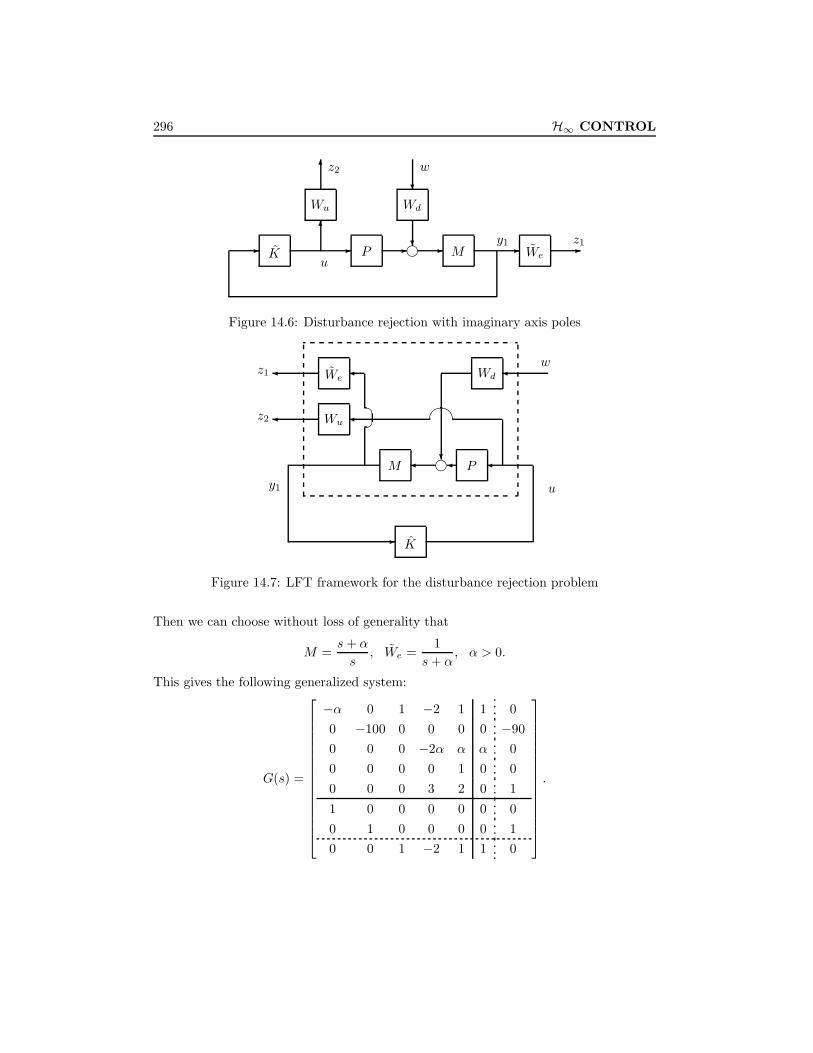
296 H∞ CONTROL
gK P
WdWu
-
?
-6
6
?M We
- - --u
wz2
y1 z1
Figure 14.6: Disturbance rejection with imaginary axis poles
gM
Wu
We Wd
K
?
-
P
z1
z2
w
uy1
Figure 14.7: LFT framework for the disturbance rejection problem
Then we can choose without loss of generality that
M =s+ α
s, We =
1s+ α
, α > 0.
This gives the following generalized system:
G(s) =
−α 0 1 −2 1 1 00 −100 0 0 0 0 −900 0 0 −2α α α 00 0 0 0 1 0 00 0 0 3 2 0 1
1 0 0 0 0 0 00 1 0 0 0 0 10 0 1 −2 1 1 0
.

14.9. H∞ Filtering 297
The suboptimal H∞ controller K∞ for each α can be computed easily as
K∞ =−2060381.4(s+ 1)(s+ α)(s + 100)(s− 0.1557)
(s+ α)2(s+ 32.17)(s+ 262343)(s− 19.89),
which gives the closed-loop H∞ norm 7.854. Hence the controller K∞ = −K∞(s)M(s)is given by
K∞(s) =2060381.4(s+ 1)(s+ 100)(s− 0.1557)s(s+ 32.17)(s+ 262343)(s− 19.89)
≈ 7.85(s+ 1)(s+ 100)(s− 0.1557)s(s+ 32.17)(s− 19.89)
,
which is independent of α as expected. Similarly, we can solve an optimal H2 controller
K2 =−43.487(s+ 1)(s+ α)(s+ 100)(s− 0.069)(s+ α)2(s2 + 30.94s+ 411.81)(s− 7.964)
and
K2(s) = −K2(s)M(s) =43.487(s+ 1)(s+ 100)(s− 0.069)s(s2 + 30.94s+ 411.81)(s− 7.964)
.
An approximate integral control can also be achieved without going through thepreceding process by letting
We = We =1
s+ ε, M(s) = 1
for a sufficiently small ε > 0. For example, a controller for ε = 0.001 is given by
K∞ =316880(s+ 1)(s+ 100)(s− 0.1545)
(s+ 0.001)(s+ 32)(s+ 40370)(s− 20)≈ 7.85(s+ 1)(s+ 100)(s− 0.1545)
s(s+ 32)(s− 20),
which gives the closed-loop H∞ norm of 7.85. Similarly, an approximate H2 integralcontroller is obtained as
K2 =43.47(s+ 1)(s+ 100)(s− 0.0679)
(s+ 0.001)(s2 + 30.93s+ 411.7)(s− 7.972)≈ 43.47(s+ 1)(s+ 100)(s− 0.0679)s(s2 + 30.93s+ 411.7)(s− 7.972)
.
14.9 H∞ Filtering
In this section we show how the filtering problem can be solved using the H∞ theorydeveloped earlier. Suppose a dynamic system is described by the following equations:
x = Ax+B1w(t), x(0) = 0 (14.18)y = C2x+D21w(t) (14.19)z = C1x+D11w(t) (14.20)
The filtering problem is to find an estimate z of z in some sense using the measurementof y. The restriction on the filtering problem is that the filter has to be causal so

298 H∞ CONTROL
that it can be realized (i.e., z has to be generated by a causal system acting on themeasurements). We will further restrict our filter to be unbiased; that is, given T > 0the estimate z(t) = 0 ∀t ∈ [0, T ] if y(t) = 0, ∀t ∈ [0, T ]. Now we can state our H∞filtering problem.
H∞ Filtering: Given a γ > 0, find a causal filter F (s) ∈ RH∞ if it existssuch that
J := supw∈L2[0,∞)
‖z − z‖22‖w‖22
< γ2
with z = F (s)y.
A diagram for the filtering problem is shown in Figure 14.8.
j A B1
C1 D11
C2 D21
F (s)
?
z∆
z
−z y
w
Figure 14.8: Filtering problem formulation
The preceding filtering problem can also be formulated in an LFT framework: Givena system shown below
G(s)
F (s)
z∆
y
w
z
-
G(s) =
A B1 0
C1 D11 −IC2 D21 0
find a filter F (s) ∈ RH∞ such that
supw∈L2
‖z∆‖22‖w‖22
< γ2. (14.21)
Hence the filtering problem can be regarded as a special H∞ problem. However, com-pared with control problems, there is no internal stability requirement in the filteringproblem. Hence the solution to the above filtering problem can be obtained from theH∞solution in the previous sections by setting B2 = 0 and dropping the internal stabilityrequirement.
Theorem 14.8 Suppose (C2, A) is detectable and[A− jωI B1
C2 D21
]

14.10. Notes and References 299
has full row rank for all ω. Let D21 be normalized and D11 partitioned conformably as[D11
D21
]=
[D111 D112
0 I
].
Then there exists a causal F (s) ∈ RH∞ such that J < γ2 if and only if σ(D111) < γand J∞ ∈ dom(Ric) with Y∞ = Ric(J∞) ≥ 0, where
R :=
[D11
D21
][D11
D21
]∗−[γ2I 00 0
]
J∞ :=
[A∗ 0
−B1B∗1 −A
]−[
C∗1 C∗2−B1D
∗11 −B1D
∗21
]R−1
[D11B
∗1 C1
D21B∗1 C2
].
Moreover, if the above conditions are satisfied, then a rational causal filter F (s)satisfying J < γ2 is given by
z = F (s)y =
[A+ L2∞C2 + L1∞D112C2 −L2∞ − L1∞D112
C1 −D112C2 D112
]y
where [L1∞ L2∞
]:= −
[B1D
∗11 + Y∞C∗1 B1D
∗21 + Y∞C∗2
]R−1.
In the case where D11 = 0 and B1D∗21 = 0 the filter becomes much simpler:
z =
[A− Y∞C∗2C2 Y∞C∗2
C1 0
]y
where Y∞ is the stabilizing solution to
Y∞A∗ +AY∞ + Y∞(γ−2C∗1C1 − C∗2C2)Y∞ +B1B
∗1 = 0.
14.10 Notes and References
The first part of this chapter is based on Sampei, Mita, and Nakamichi [1990], Packard[1994], Doyle, Glover, Khargonekar, and Francis [1989], and Chen and Zhou [1996].The proof of Theorem 14.4 comes from Ran and Vreugdenhil [1988]. The detailedderivation of the H∞ solution for the general case is treated in Glover and Doyle [1988,1989]. A fairly complete solution to the singular H∞ problem is obtained in Stoorvogel[1992]. The H∞ filtering and smoothing problems are considered in detail in Nagpaland Khargonekar [1991]. There is a rich body of literature on the LMI approach to H∞control and related problems. In particular, readers are referred to the monograph byBoyd, Ghaoui, Feron, and Balakrishnan [1994] for a comprehensive treatment of LMIsand their applications in control. See also the paper by Chilali and Gahinet [1996] foran application of LMIs in H∞ control with closed-loop pole constraints.

300 H∞ CONTROL
14.11 Problems
Problem 14.1 Figure 14.9 shows a single-loop analog feedback system. The plant is
F K P
W ε2 ε1
j j- - - - - -
6
6 6
6 6
?
?w1 e y u
z1 w2 z2
−
Figure 14.9: Analog feedback system
P and the controller K; F is an antialiasing filter for future digital implementation ofthe controller (it is a good idea to include F at the start of the analog design so thatthere are no surprises later due to additional phase lag). The basic control specificationis to get good tracking over a certain frequency range, say [0, ω1]; that is, to make themagnitude of the transfer function from w1 to e small over this frequency range. Theweighted tracking error is z1 in the figure, where the weight W is selected to be a low-pass filter with bandwidth ω1. We could attempt to minimize the H∞ norm from w1
to z1, but this problem is not regular. To regularize it, another input, w2, is added andanother signal, z2, is penalized. The two weights ε1 and ε2 are small positive scalars.The design problem is to minimize the H∞ norm
from w =
[w1
w2
]to z =
[z1
z2
].
Figure 14.9 can then be converted to the standard setup by stacking the states of P , F ,and W to form the state of G.
The plant transfer function is taken to be
P (s) =20− s
(s+ 0.01)(s+ 20).
With a view toward subsequent digital control with h = 0.5, the filter F is taken tohave bandwidth π/0.5, and Nyquist frequency ωN :
F (s) =1
(0.5/π)s+ 1.

14.11. Problems 301
The weight W is then taken to have bandwidth one-fifth the Nyquist frequency:
W (s) =[
1(2.5/π)s+ 1
]2
.
Finally, ε1 and ε2 are both set to 0.01.Run hinfsyn and show your plots of the closed-loop frequency responses.
Problem 14.2 Make the same assumptions as in Chapter 13 for H2 control and derivethe H∞ controller parameterization by using the normalization procedure and Theo-rem 14.7.
Problem 14.3 Consider the feedback system in Figure 6.3 and suppose
P =s− 10
(s+ 1)(s+ 10), We =
1s+ 0.001
, Wu =s+ 2s+ 10
.
Design a controller that minimizes∥∥∥∥∥[
WeSo
WuKSo
]∥∥∥∥∥∞
.
Simulate the time response of the system when r is a step.
Problem 14.4 Repeat Problem 14.3 when We = 1/s.
Problem 14.5 Consider again Problem 13.5 and design a controller that minimizesthe H∞ norm of the transfer matrix from r to (e, uw).
Problem 14.6 Repeat Problem 14.5 with W = ε for ε = 0.01 and 0.0001. Study thebehavior of the controller when ε→ 0.
Problem 14.7 Repeat Problem 14.5 and Problem 14.6 with
P =10(2− s)(s+ 1)3
.
Problem 14.8 Let N ∈ RH−∞. The Nehari problem is the following approximationproblem:
infQ∈RH∞
‖N −Q‖∞ .
Formulate the Nehari problem as a standard H∞ control problem.
Problem 14.9 Consider a generalized plant
P =
−4 25 0.8 −1−10 29 0.9 −1
10 −25 0 113 25 1 0

302 H∞ CONTROL
with an SISO controller K. Find the optimal H∞ performance γopt. Calculate thecentral controller for each γ ∈ (γopt, 2) and the corresponding H∞ performance, γ∞.Plot γ∞ versus γ. Is γ∞ monotonic with respect to γ? (See Ushida and Kimura [1996]for a detailed discussion.)
Problem 14.10 Let a satellite model be given by Po(s) =
[A B
C 0
], where
A =
0 1 0 00 0 0 00 0 0 10 0 −1.5392 −2× 0.003× 1.539
, B =
0
1.7319× 10⁻⁵
03.7859× 10⁻⁴
,
C =[
1 0 1 0], D = 0.
Suppose the true system is described by
P = (N + ∆N )(M + ∆M )−1
where Po = NM−1 is a normalized coprime factorization. Design a controller so thatthe controller stabilizes the largest
∆ =
[∆N
∆M
].
Problem 14.11 Consider the feedback system shown below and let
P =0.5(1− s)
(s+ 2)(s+ 0.5), W1 = 50
s/1.245 + 1s/0.007 + 1
, W2 = 0.1256s/0.502 + 1s/2 + 1
.
e eK P
W2 ∆
W1- - -
CCCCW ?
-
-
-
-6−
w2z1 w1
z2
Figure 14.10: System with additive uncertainty
Then [z1
z2
]=
[−W2KS −W2KS
W1S W1S
][w1
w2
]= M
[w1
w2
]where S = (I + PK)−1.

14.11. Problems 303
(a) Design a controller K such that
infK stabilizing
‖M‖∞ .
(b) Design a controller K so that
infK stabilizing
supωµ∆(M), ∆ =
[∆1
∆2
].
Note that µ∆(M) = |W1S|+ |W2KS|.
Problem 14.12 Design a µ-synthesis controller for the HIMAT control problem inExample 9.1.
Problem 14.13 Let G(s) ∈ H∞ be a square transfer matrix and α > 0. Show that Gis (extended) strictly positive real (i.e., G∗(jω) + G(jω) > 0, ∀ ω ∈ R ∪ ∞) if andonly if
∥∥(αI −G)(αI +G)−1∥∥∞ < 1.
Problem 14.14 Consider a generalized system
G(s) =
A B1 B2
C1 D11 D12
C2 D21 D22
and suppose we want to find a controller K such that F`(G,K) is (extended) strictlypostive real. Show that the problem can be converted to a standardH∞ control problemby using the transformation in the last problem.
Problem 14.15 (Synthesis Using Popov Criterion) A stability criterion by Popov in-volves finding a controller and a multiplier matrix N such that
Q+ (I + sN)F`(G,K)
is strictly positive real where Q is a constant matrix. Assume D11 = 0 and D12 = 0 inthe realization of G. Find the G so that
Q+ (I + sN)F`(G,K) = F`(G,K)
Hence the results in the last problem can be applied.

304 H∞ CONTROL

Chapter 15
Controller Reduction
We have shown in the previous chapters that the H∞ control theory and µ synthesiscan be used to design robust performance controllers for highly complex uncertain sys-tems. However, since a great many physical plants are modeled as high-order dynamicalsystems, the controllers designed with these methodologies typically have orders com-parable to those of the plants. Simple linear controllers are normally preferred overcomplex linear controllers in control system designs for some obvious reasons: Theyare easier to understand and computationally less demanding; they are also easier toimplement and have higher reliability since there are fewer things to go wrong in thehardware or bugs to fix in the software. Therefore, a lower-order controller should besought whenever the resulting performance degradation is kept within an acceptablelevel. There are usually three ways to arrive at a lower-order controller. A seeminglyobvious approach is to design lower-order controllers directly based on the high-ordermodels. However, this is still largely an open research problem. Another approach isfirst to reduce the order of a high-order plant and, second, based on the reduced plantmodel, design a lower-order controller. A potential problem associated with this ap-proach is that such a lower-order controller may not even stabilize the full-order plantsince the error information between the full-order model and the reduced-order modelis not considered in the design of the controller. On the other hand, one may seek todesign first a high-order, high-performance controller and subsequently proceed with areduction of the designed controller. This approach is usually referred to as controllerreduction. A crucial consideration in controller order reduction is to take into accountthe closed loop so that closed-loop stability is guaranteed and the performance degrada-tion is minimized with the reduced-order controllers. The purpose of this chapter is tointroduce several controller reduction methods that can guarantee closed-loop stabilityand possibly closed-loop performance as well.
305

306 CONTROLLER REDUCTION
15.1 H∞ Controller Reductions
In this section, we consider an H∞ performance-preserving controller order reductionproblem. We consider the feedback system shown in Figure 15.1 with a generalizedplant realization given by
G(s) =
A B1 B2
C1 D11 D12
C2 D21 D22
.
G(s)
K(s)
z
y
w
u
-
Figure 15.1: Closed-loop system diagram
The following assumptions are made:
(A1) (A,B2) is stabilizable and (C2, A) is detectable;
(A2) D12 has full column rank and D21 has full row rank;
(A3)
[A− jωI B2
C1 D12
]has full column rank for all ω;
(A4)
[A− jωI B1
C2 D21
]has full row rank for all ω.
As stated in Chapter 14, all stabilizing controllers satisfying ‖Tzw‖∞ < γ can be pa-rameterized as
K = F`(M∞, Q), Q ∈ RH∞, ‖Q‖∞ < γ (15.1)
where M∞ is of the form
M∞ =
[M11(s) M12(s)M21(s) M22(s)
]=
A B1 B2
C1 D11 D12
C2 D21 D22
such that D12 and D21 are invertible and A − B2D
−112 C1 and A − B1D
−121 C2 are both
stable (i.e., M−112 and M−1
21 are both stable).

15.1. H∞ Controller Reductions 307
The problem to be considered here is to find a controller K with a minimal possibleorder such that the H∞ performance requirement
∥∥∥F`(G, K)∥∥∥∞< γ is satisfied. This is
clearly equivalent to finding aQ so that it satisfies the preceding constraint and the orderof K is minimized. Instead of choosing Q directly, we shall approach this problem froma different perspective. The following lemma is useful in the subsequent developmentand can be regarded as a special case of Theorem 10.6 (main loop theorem).
Lemma 15.1 Consider a feedback system shown below
N
Q
z
y
w
u
-
where N is a suitably partitioned transfer matrix
N(s) =
[N11 N12
N21 N22
].
Then the closed-loop transfer matrix from w to z is given by
Tzw = F`(N,Q) = N11 +N12Q(I −N22Q)−1N21.
Assume that the feedback loop is well-posed [i.e., det(I −N22(∞)Q(∞)) 6= 0] and eitherN21(jω) has full row rank for all ω ∈ R ∪ ∞ or N12(jω) has full column rank for allω ∈ R ∪∞ and ‖N‖∞ ≤ 1; then ‖F`(N,Q)‖∞ < 1 if ‖Q‖∞ < 1.
Proof. We shall assume that N21 has full row rank. The case when N12 has fullcolumn rank can be shown in the same way.
To show that ‖Tzw‖∞ < 1, consider the closed-loop system at any frequency s = jωwith the signals fixed as complex constant vectors. Let ‖Q‖∞ =: ε < 1 and note thatTwy = N+
21(I−N22Q), where N+21 is a right inverse of N21. Also let κ := ‖Twy‖∞. Then
‖w‖2 ≤ κ‖y‖2, and ‖N‖∞ ≤ 1 implies that ‖z‖22 + ‖y‖22 ≤ ‖w‖22 + ‖u‖22. Therefore,
‖z‖22 ≤ ‖w‖22 + (ε2 − 1)‖y‖22 ≤ [1− (1− ε2)κ−2]‖w‖22,
which implies ‖Tzw‖∞ < 1 . 2

308 CONTROLLER REDUCTION
15.1.1 Additive Reduction
Consider the class of (reduced-order) controllers that can be represented in the form
K = K0 +W2∆W1,
where K0 may be interpreted as a nominal, higher-order controller, and ∆ is a stableperturbation with stable, minimum phase and invertible weighting functions W1 andW2. Suppose that ‖F`(G,K0)‖∞ < γ. A natural question is whether it is possible toobtain a reduced-order controller K in this class such that the H∞ performance boundremains valid when K is in place of K0. Note that this is somewhat a special case of thepreceding general problem: The specific form of K means that K and K0 must possessthe same right-half plane poles, thus to a certain degree limiting the set of attainablereduced-order controllers.
Suppose K is a suboptimal H∞ controller; that is, there is a Q ∈ RH∞ with‖Q‖∞ < γ such that K = F`(M∞, Q). It follows from simple algebra that
Q = F`(K−1a , K)
where
K−1a :=
[0 I
I 0
]M−1∞
[0 I
I 0
].
Furthermore, it follows from straightforward manipulations that
‖Q‖∞ < γ ⇐⇒∥∥∥F`(K−1
a , K)∥∥∥∞< γ
⇐⇒∥∥F`(K−1
a ,K0 +W2∆W1)∥∥∞ < γ
⇐⇒∥∥∥F`(R,∆)
∥∥∥∞< 1
where
R =
[γ−1/2I 0
0 W1
][R11 R12
R21 R22
][γ−1/2I 0
0 W2
]and R is given by the star product[
R11 R12
R21 R22
]= S(K−1
a ,
[Ko I
I 0
]).
It is easy to see that R12 and R21 are both minimum phase and invertible and hencehave full column and full row rank, respectively, for all ω ∈ R ∪ ∞. Consequently,by invoking Lemma 15.1, we conclude that if R is a contraction and ‖∆‖∞ < 1, then∥∥∥F`(R,∆)
∥∥∥∞
< 1. This guarantees the existence of a Q such that ‖Q‖∞ < γ or,
equivalently, the existence of a K such that∥∥∥F`(G, K)
∥∥∥∞< γ. This observation leads
to the following theorem.

15.1. H∞ Controller Reductions 309
Theorem 15.2 Suppose W1 and W2 are stable, minimum phase and invertible transfermatrices such that R is a contraction. Let K0 be a stabilizing controller such that‖F`(G,K0)‖∞ < γ. Then K is also a stabilizing controller such that
∥∥∥F`(G, K)∥∥∥∞< γ
if‖∆‖∞ =
∥∥∥W−12 (K −K0)W−1
1
∥∥∥∞< 1.
Since R can always be made contractive for sufficiently small W1 and W2, there areinfinite many W1 and W2 that satisfy the conditions in the theorem. It is obvious thatto make
∥∥∥W−12 (K −K0)W−1
1
∥∥∥∞< 1 for some K, one would like to select the “largest”
W1 and W2 such that R is a contraction.
Lemma 15.3 Assume that ‖R22‖∞ < γ and define
L =
[L1 L2
L∼2 L3
]= F`(
0 −R11 0 R12
−R∼11 0 R∼21 00 R21 0 −R22
R∼12 0 −R∼22 0
, γ−1I).
Then R is a contraction if W1 and W2 satisfy[(W∼1 W1)−1 0
0 (W2W∼2 )−1
]≥[L1 L2
L∼2 L3
].
Proof. See Goddard and Glover [1993]. 2
An algorithm that maximizes det(W∼1 W1) det(W2W∼2 ) has been developed by God-
dard and Glover [1993]. The procedure below, devised directly from the precedingtheorem, can be used to generate a required reduced-order controller that will preservethe closed-loop H∞ performance bound
∥∥∥F`(G, K)∥∥∥∞< γ.
1. Let K0 be a full-order controller such that ‖F`(G,K0)‖∞ < γ;
2. Compute W1 and W2 so that R is a contraction;
3. Use the weighted model reduction method in Chapter 7 or any other methods tofind a K so that
∥∥∥W−12 (K −K0)W−1
1
∥∥∥∞< 1.
Note that all controller reduction methods introduced in this book are only sufficient;that is, there may be desired reduced-order controllers that cannot be found from theproposed procedures.

310 CONTROLLER REDUCTION
15.1.2 Coprime Factor Reduction
The H∞ controller reduction problem can also be considered in the coprime factorframework. For that purpose, we need the following alternative representation of alladmissible H∞ controllers:
Lemma 15.4 The family of all admissible controllers such that ‖Tzw‖∞ < γ can alsobe written as
K(s) = F`(M∞, Q) = (Θ11Q+ Θ12)(Θ21Q+ Θ22)−1 := UV −1
= (QΘ12 + Θ22)−1(QΘ11 + Θ21) := V −1U
where Q ∈ RH∞, ‖Q‖∞ < γ, and UV −1 and V −1U are, respectively, right and leftcoprime factorizations over RH∞, and
Θ =
[Θ11 Θ12
Θ21 Θ22
]=
A− B1D−121 C2 B2 − B1D
−121 D22 B1D
−121
C1 − D11D−121 C2 D12 − D11D
−121 D22 D11D
−121
−D−121 C2 −D−1
21 D22 D−121
Θ =
[Θ11 Θ12
Θ21 Θ22
]=
A− B2D−112 C1 B1 − B2D
−112 D11 −B2D
−112
C2 − D22D−112 C1 D21 − D22D
−112 D11 −D22D
−112
D−112 C1 D−1
12 D11 D−112
Θ−1 =
A− B2D−112 C1 B2D
−112 B1 − B2D
−112 D11
−D−112 C1 D−1
12 −D−112 D11
C2 − D22D−112 C1 D22D
−112 D21 − D22D
−112 D11
Θ−1 =
A− B1D−121 C2 −B1D
−121 B2 − B1D
−121 D22
D−121 C2 D−1
21 D−121 D22
C1 − D11D−121 C2 −D11D
−121 D12 − D11D
−121 D22
.Proof. The results follow immediately from Lemma 9.2. 2
Theorem 15.5 Let K0 = Θ12Θ−122 be the central H∞ controller such that
‖F`(G,K0)‖∞ < γ and let U , V ∈ RH∞ with det V (∞) 6= 0 be such that∥∥∥∥∥[γ−1I 0
0 I
]Θ−1
([Θ12
Θ22
]−[U
V
])∥∥∥∥∥∞
< 1/√
2. (15.2)
Then K = U V −1 is also a stabilizing controller such that ‖F`(G, K)‖∞ < γ.

15.1. H∞ Controller Reductions 311
Proof. Note that by Lemma 15.4, K is an admissible controller such that ‖Tzw‖∞ < γif and only if there exists a Q ∈ RH∞ with ‖Q‖∞ < γ such that[
U
V
]:=
[Θ11Q+ Θ12
Θ21Q+ Θ22
]= Θ
[Q
I
](15.3)
andK = UV −1.
Hence, to show that K = U V −1 with U and V satisfying equation (15.2) is also astabilizing controller such that ‖F`(G, K)‖∞ < γ, we need to show that there is anothercoprime factorization for K = UV −1 and a Q ∈ RH∞ with ‖Q‖∞ < γ such thatequation (15.3) is satisfied.
Define
∆ :=
[γ−1I 0
0 I
]Θ−1
([Θ12
Θ22
]−[U
V
])and partition ∆ as
∆ :=
[∆U
∆V
].
Then [U
V
]=
[Θ12
Θ22
]−Θ
[γI 00 I
]∆ = Θ
[−γ∆U
I −∆V
]and [
U(I −∆V )−1
V (I −∆V )−1
]= Θ
[−γ∆U(I −∆V )−1
I
].
Define U := U(I−∆V )−1, V := V (I−∆V )−1, and Q := −γ∆U(I−∆V )−1. Then UV −1
is another coprime factorization for K. To show that K = UV −1 = U V −1 is a stabilizingcontroller such that ‖F`(G, K)‖∞ < γ, we need to show that
∥∥γ∆U(I −∆V )−1∥∥∞ < γ
or, equivalently,∥∥∆U (I −∆V )−1
∥∥∞ < 1. Now
∆U(I −∆V )−1 =[I 0
]∆(I −
[0 I
]∆)−1
= F`
0[I 0
]I/√
2[
0 I/√
2] ,√2∆
and, by Lemma 15.1,
∥∥∆U(I −∆V )−1∥∥∞ < 1 since 0[I 0
]I/√
2[
0 I/√
2]

312 CONTROLLER REDUCTION
is a contraction and∥∥√2∆
∥∥∞ < 1. 2
Similarly, we have the following theorem:
Theorem 15.6 Let K0 = Θ−122 Θ21 be the central H∞ controller such that
‖F`(G,K0)‖∞ < γ and let ˆU, ˆV ∈ RH∞ with det ˆV (∞) 6= 0 be such that∥∥∥∥∥([ Θ21 Θ22
]−[
ˆU ˆV])
Θ−1
[γ−1I 0
0 I
]∥∥∥∥∥∞
< 1/√
2.
Then K = ˆV−1 ˆU is also a stabilizing controller such that ‖F`(G, K)‖∞ < γ.
The preceding two theorems show that the sufficient conditions for H∞ controllerreduction problem are equivalent to frequency-weighted H∞ model reduction problems.
H∞ Controller Reduction Procedures
(i) Let K0 = Θ12Θ−122 (= Θ−1
22 Θ21) be a suboptimal H∞ central controller (Q = 0) suchthat ‖Tzw‖∞ < γ.
(ii) Find a reduced-order controller K = U V −1 (or ˆV−1 ˆU) such that∥∥∥∥∥
[γ−1I 0
0 I
]Θ−1
([Θ12
Θ22
]−[U
V
])∥∥∥∥∥∞
< 1/√
2
or ∥∥∥∥∥([ Θ21 Θ22
]−[
ˆU ˆV])
Θ−1
[γ−1I 0
0 I
]∥∥∥∥∥∞
< 1/√
2.
Then the closed-loop system with the reduced-order controller K is stable and theperformance is maintained with the reduced-order controller; that is,
‖Tzw‖∞ =∥∥∥F`(G, K)
∥∥∥∞< γ.
15.2 Notes and References
The main results presented in this chapter are based on the work of Goddard andGlover [1993, 1994]. Other controller reduction methods include the stability-orientedcontroller reduction criterion proposed by Enns [1984a, 1984b]; the weighted and un-weighted coprime factor controller reduction methods studied by Liu and Anderson[1986, 1990]; Liu, Anderson, and Ly [1990]; Anderson and Liu [1989]; and Anderson[1993]; the normalized H∞ controller reduction studied by Mustafa and Glover [1991];the normalized coprime factor method studied by McFarlane and Glover [1990] in theH∞ loop-shaping setup; and the controller reduction in the ν-gap metric setup studiedby Vinnicombe [1993b]. Lenz, Khargonekar, and Doyle [1987] have also proposed an-other H∞ controller reduction method with guaranteed performance for a class of H∞problems.

15.3. Problems 313
15.3 Problems
Problem 15.1 Find a lower-order controller for the system in Example 10.4 whenγ = 2.
Problem 15.2 Find a lower-order controller for Problem 14.3 when γ = 1.1γopt whereγopt is the optimal norm.
Problem 15.3 Find a lower-order controller for the HIMAT control problem in Prob-lem 14.12 when γ = 1.1γopt where γopt is the optimal norm. Compare the controllerreduction methods presented in this chapter with other available methods.
Problem 15.4 Let G be a generalized plant and K be a stabilizing controller. Let∆ = diag(∆p,∆k) be a suitably dimensioned perturbation and let Tzw be the transfer
matrix from w =
[w
w1
]to z =
[z
z1
]in the following diagram:
fG
K
-
-
(K −K)W
W−1
-
zw
z w
z1 w1
Let W,W−1 ∈ H∞ be a given transfer matrix. Show that the following statements areequivalent:
1. µ∆
([I 00 W−1
]Tzw
)< 1;
2. ‖F`(G,K)‖∞ < 1 and∥∥W−1Fu(Tzw,∆p)
∥∥∞ < 1 for all σ(∆p) ≤ 1;
3.∥∥W−1Tz1w1
∥∥∞ < 1 and
∥∥∥∥∥F`([
I 00 W−1
]Tzw,∆k
)∥∥∥∥∥∞
< 1 for all σ(∆k) ≤ 1.
Problem 15.5 In the part 3 of Problem 15.4, if we let ∆k = (K−K)W , then Tz1w1 =
G22(I −KG22)−1 and F`
([I 00 W−1
]Tzw,∆k
)= F`(G, K). Thus K stabilizes the
system and satisfies∥∥∥F`(G, K)
∥∥∥∞< 1 if ‖∆k‖∞ =
∥∥∥(K −K)W∥∥∥∞≤ 1 and part 2 of

314 CONTROLLER REDUCTION
Problem 15.4 is satisfied by a controller K. Hence to reduce the order of the controllerK, it is sufficient to solve a frequency-weighted model reduction problem if W can becalculated. In the single-input and single-output case, a “smallest” weighting functionW (s) can be calculated using part 2 of Problem 15.4 as follows:
|W (jω)| ≥ supσ(∆p)≤1
|Fu(Tzw(jω),∆p)|.
Repeat Problems 15.1 and 15.2 using the foregoing method. (Hint: W can be computedfrequency by frequency using µ software and then fitted by a stable and minimum phasetransfer function.)
Problem 15.6 One way to generalize the method in Problem 15.5 to the MIMO caseis to take a diagonal W
W = diag(W1,W2, . . . ,Wm)
and let Wi be computed from
|Wi(jω)| ≥ supσ(∆p)≤1
∥∥eTi Fu(Tzw(jω),∆p)∥∥
where ei is the ith unit vector. Next let α(s) be computed from
|α(jω)| ≥ supσ(∆p)≤1
∥∥∥W−1Fu(Tzw(jω),∆p)∥∥∥
where W = diag(W1, W2, . . . , Wm). Then a suitable W can be taken as
W = αW .
Apply this method to Problem 15.3.
Problem 15.7 Generalize the procedures in Problems 15.5 and 15.6 to problems withadditional structured uncertainty cases. (A more general case can be found in Yang andPackard [1995].)

Chapter 16
H∞ Loop Shaping
This chapter introduces a design technique that incorporates loop-shaping methods toobtain performance/robust stability tradeoffs, and a particular H∞ optimization prob-lem to guarantee closed-loop stability and a level of robust stability at all frequencies.The proposed technique uses only the basic concept of loop-shaping methods, and thena robust stabilization controller for the normalized coprime factor perturbed system isused to construct the final controller. This chapter is arranged as follows: The H∞theory is applied to solve the stabilization problem of a normalized coprime factorperturbed system in Section 16.1. The loop-shaping design procedure is described inSection 16.2. The theoretical justification for the loop-shaping design procedure is givenin Section 16.3. Some further loop-shaping guidelines are given in Section 16.4.
16.1 Robust Stabilization of Coprime Factors
In this section, we use the H∞ control theory developed in previous chapters to solvethe robust stabilization of a left coprime factor perturbed plant given by
P∆ = (M + ∆M )−1(N + ∆N )
with M, N, ∆M , ∆N ∈ RH∞ and∥∥∥[ ∆N ∆M
]∥∥∥∞< ε (see Figure 16.1). The transfer
matrices (M, N) are assumed to be a left coprime factorization of P (i.e., P = M−1N),and K internally stabilizes the nominal system.
It has been shown in Chapter 8 that the system is robustly stable iff∥∥∥∥∥[K
I
](I + PK)−1M−1
∥∥∥∥∥∞
≤ 1/ε.
Finding a controller such that the above norm condition holds is an H∞ norm mini-mization problem that can be solved using H∞ theory developed in previous chapters.
315

316 H∞ LOOP SHAPING
fff
−
−
yw
z2z1
r
6
?
-
∆M
M−1--
-
N
∆N-
-K--
Figure 16.1: Left coprime factor perturbed systems
Suppose P has a stabilizable and detectable state-space realization given by
P =
[A B
C D
]and let L be a matrix such that A+ LC is stable. Then a left coprime factorization ofP = M−1N is given by[
N M]
=
[A+ LC B + LD L
ZC ZD Z
]where Z can be any nonsingular matrix. In particular, we shall choose Z = (I +DD∗)−1/2 if P = M−1N is chosen to be a normalized left coprime factorization. Denote
K = −K.
Then the system diagram can be put in an LFT form, as in Figure 16.2, with thegeneralized plant
G(s) =
[
0M−1
] [I
P
]M−1 P
=
A −LZ−1 B[0C
] [0
Z−1
] [I
D
]C Z−1 D
=:
A B1 B2
C1 D11 D12
C2 D21 D22
.To apply the H∞ control formulas in Chapter 14, we need to normalize the D12 and
D21 first. Note that[I
D
]= U
[0I
](I +D∗D)
12 , where U =
[D∗(I +DD∗)−
12 (I +D∗D)−
12
−(I +DD∗)−12 D(I +D∗D)−
12
]

16.1. Robust Stabilization of Coprime Factors 317
iM−1
K
N ?
-
uy
z1
z2
w
Figure 16.2: LFT diagram for coprime factor stabilization
and U is a unitary matrix. Let
K = (I +D∗D)−12 KZ[
z1
z2
]= U
[z1
z2
].
Then ‖Tzw‖∞ = ‖U∗Tzw‖∞ = ‖Tzw‖∞ and the problem becomes one of finding acontroller K so that ‖Tzw‖∞ < γ with the following generalized plant:
G =
[U∗ 00 Z
]G
[I 00 (I +D∗D)−
12
]
=
A −LZ−1 B[
−(I +DD∗)−12C
(I +D∗D)−12D∗C
] [−(I +DD∗)−
12Z−1
(I +D∗D)−12D∗Z−1
] [0I
]ZC I ZD(I +D∗D)−
12
.Now the formulas in Chapter 14 can be applied to G to obtain a controller K and thenthe K can be obtained from K = −(I +D∗D)−
12 KZ. We shall leave the detail to the
reader. In the sequel, we shall consider the case D = 0 and Z = I. In this case, we haveγ > 1 and
X∞(A− LC
γ2 − 1) + (A− LC
γ2 − 1)∗X∞ −X∞(BB∗ − LL∗
γ2 − 1)X∞ +
γ2C∗C
γ2 − 1= 0
Y∞(A+ LC)∗ + (A+ LC)Y∞ − Y∞C∗CY∞ = 0.

318 H∞ LOOP SHAPING
It is clear that Y∞ = 0 is the stabilizing solution. Hence by the formulas in Chapter 14we have [
L1∞ L2∞
]=[
0 L]
and
Z∞ = I, D11 = 0, D12 = I, D21 =
√γ2 − 1γ
I.
The results are summarized in the following theorem.
Theorem 16.1 Let D = 0 and let L be such that A + LC is stable. Then there existsa controller K such that ∥∥∥∥∥
[K
I
](I + PK)−1M−1
∥∥∥∥∥∞
< γ
iff γ > 1 and there exists a stabilizing solution X∞ ≥ 0 solving
X∞(A− LC
γ2 − 1) + (A− LC
γ2 − 1)∗X∞ −X∞(BB∗ − LL∗
γ2 − 1)X∞ +
γ2C∗C
γ2 − 1= 0.
Moreover, if the above conditions hold a central controller is given by
K =
[A−BB∗X∞ + LC L
−B∗X∞ 0
].
It is clear that the existence of a robust stabilizing controller depends on the choice ofthe stabilizing matrix L (i.e., the choice of the coprime factorization). Now let Y ≥ 0be the stabilizing solution to
AY + Y A∗ − Y C∗CY +BB∗ = 0
and let L = −Y C∗. Then the left coprime factorization (M, N) given by[N M
]=
[A− Y C∗C B −Y C∗
C 0 I
]is a normalized left coprime factorization (see Chapter 12). Let ‖·‖H denote the Hankelnorm (i.e., the largest Hankel singular value). Then we have the following result.
Corollary 16.2 Let D = 0 and L = −Y C∗, where Y ≥ 0 is the stabilizing solution to
AY + Y A∗ − Y C∗CY +BB∗ = 0.
Then P = M−1N is a normalized left coprime factorization and
infK stabilizing
∥∥∥∥∥[K
I
](I + PK)−1M−1
∥∥∥∥∥∞
=1√
1− λmax(Y Q)
=(
1−∥∥∥[ N M
]∥∥∥2
H
)−1/2
=: γmin

16.1. Robust Stabilization of Coprime Factors 319
where Q is the solution to the following Lyapunov equation:
Q(A− Y C∗C) + (A− Y C∗C)∗Q+ C∗C = 0.
Moreover, if the preceding conditions hold, then for any γ > γmin a controller achieving∥∥∥∥∥[K
I
](I + PK)−1M−1
∥∥∥∥∥∞
< γ
is given by
K(s) =
[A−BB∗X∞ − Y C∗C −Y C∗
−B∗X∞ 0
]where
X∞ =γ2
γ2 − 1Q
(I − γ2
γ2 − 1Y Q
)−1
.
Proof. Note that the Hamiltonian matrix associated with X∞ is given by
H∞ =
[A+ 1
γ2−1Y C∗C −BB∗ + 1
γ2−1Y C∗CY
− γ2
γ2−1C∗C −(A+ 1
γ2−1Y C∗C)∗
].
Straightforward calculation shows that
H∞ =
[I − γ2
γ2−1Y
0 γ2
γ2−1I
]Hq
[I − γ2
γ2−1Y
0 γ2
γ2−1I
]−1
where
Hq =
[A− Y C∗C 0−C∗C −(A− Y C∗C)∗
].
It is clear that the stable invariant subspace of Hq is given by
X−(Hq) = Im
[I
Q
]and the stable invariant subspace of H∞ is given by
X−(H∞) =
[I − γ2
γ2−1Y
0 γ2
γ2−1I
]X−(Hq) = Im
[I − γ2
γ2−1Y Qγ2
γ2−1Q
].
Hence there is a nonnegative definite stabilizing solution to the algebraic Riccati equa-tion of X∞ if and only if
I − γ2
γ2 − 1Y Q > 0

320 H∞ LOOP SHAPING
orγ >
1√1− λmax(Y Q)
and the solution, if it exists, is given by
X∞ =γ2
γ2 − 1Q
(I − γ2
γ2 − 1Y Q
)−1
.
Note that Y and Q are the controllability Gramian and the observability Gramian of[N M
]respectively. Therefore, we also have that the Hankel norm of
[N M
]is√λmax(Y Q). 2
Corollary 16.3 Let P = M−1N be a normalized left coprime factorization and
P∆ = (M + ∆M )−1(N + ∆N )
with ∥∥∥[ ∆N ∆M
]∥∥∥∞< ε.
Then there is a robustly stabilizing controller for P∆ if and only if
ε ≤√
1− λmax(Y Q) =
√1−
∥∥∥[ N M]∥∥∥2
H.
The solutions to the normalized left coprime factorization stabilization problem arealso solutions to a related H∞ problem, which is shown in the following lemma.
Lemma 16.4 Let P = M−1N be a normalized left coprime factorization. Then∥∥∥∥∥[K
I
](I + PK)−1M−1
∥∥∥∥∥∞
=
∥∥∥∥∥[K
I
](I + PK)−1
[I P
]∥∥∥∥∥∞
.
Proof. Since (M, N) is a normalized left coprime factorization of P , we have[M N
] [M N
]∼= I
and ∥∥∥[ M N]∥∥∥∞
=∥∥∥[ M N
]∼∥∥∥∞
= 1.
Using these equations, we have∥∥∥∥∥[K
I
](I + PK)−1M−1
∥∥∥∥∥∞
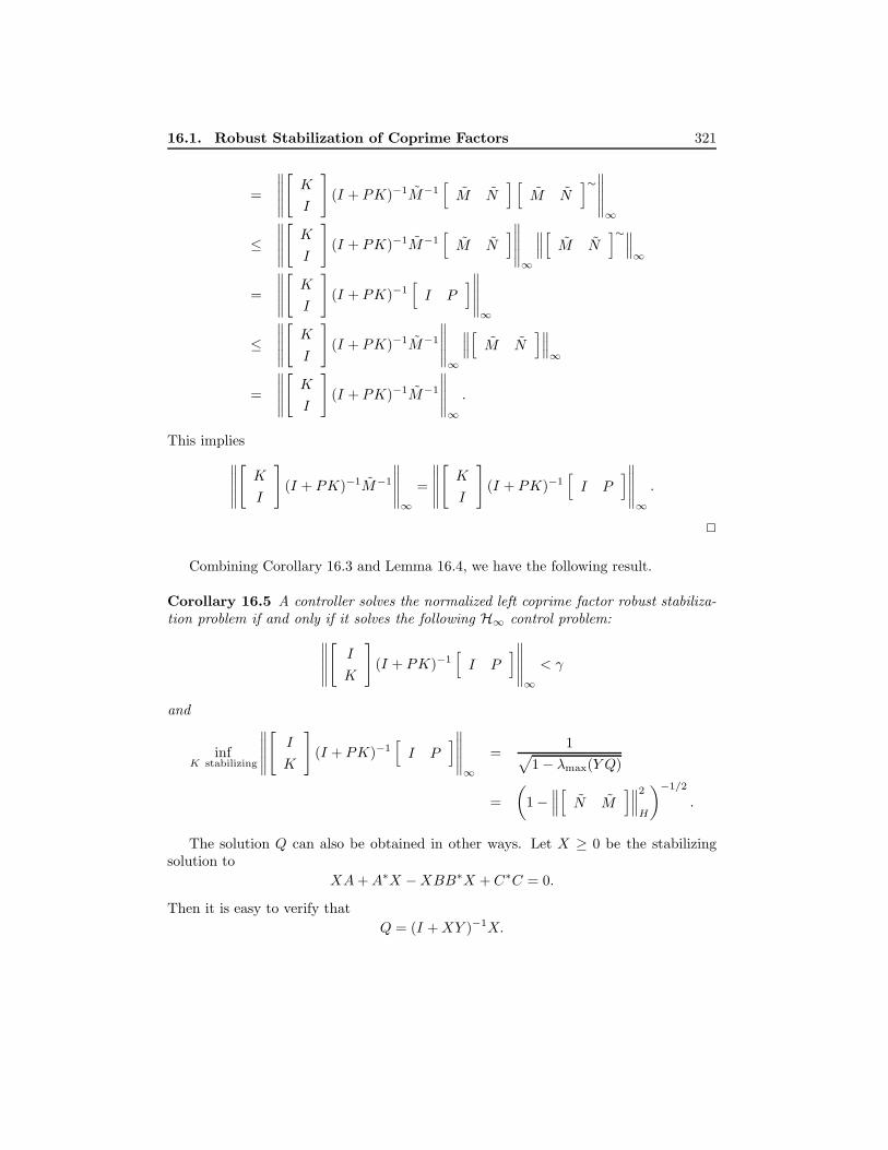
16.1. Robust Stabilization of Coprime Factors 321
=
∥∥∥∥∥[K
I
](I + PK)−1M−1
[M N
] [M N
]∼∥∥∥∥∥∞
≤∥∥∥∥∥[K
I
](I + PK)−1M−1
[M N
]∥∥∥∥∥∞
∥∥∥[ M N]∼∥∥∥
∞
=
∥∥∥∥∥[K
I
](I + PK)−1
[I P
]∥∥∥∥∥∞
≤∥∥∥∥∥[K
I
](I + PK)−1M−1
∥∥∥∥∥∞
∥∥∥[ M N]∥∥∥∞
=
∥∥∥∥∥[K
I
](I + PK)−1M−1
∥∥∥∥∥∞
.
This implies∥∥∥∥∥[K
I
](I + PK)−1M−1
∥∥∥∥∥∞
=
∥∥∥∥∥[K
I
](I + PK)−1
[I P
]∥∥∥∥∥∞
.
2
Combining Corollary 16.3 and Lemma 16.4, we have the following result.
Corollary 16.5 A controller solves the normalized left coprime factor robust stabiliza-tion problem if and only if it solves the following H∞ control problem:∥∥∥∥∥
[I
K
](I + PK)−1
[I P
]∥∥∥∥∥∞
< γ
and
infK stabilizing
∥∥∥∥∥[I
K
](I + PK)−1
[I P
]∥∥∥∥∥∞
=1√
1− λmax(Y Q)
=(
1−∥∥∥[ N M
]∥∥∥2
H
)−1/2
.
The solution Q can also be obtained in other ways. Let X ≥ 0 be the stabilizingsolution to
XA+A∗X −XBB∗X + C∗C = 0.
Then it is easy to verify thatQ = (I +XY )−1X.

322 H∞ LOOP SHAPING
Hence
γmin =1√
1− λmax(Y Q)=(
1−∥∥∥[ N M
]∥∥∥2
H
)−1/2
=√
1 + λmax(XY ).
Similar results can be obtained if one starts with a normalized right coprime factoriza-tion. In fact, a rather strong relation between the normalized left and right coprimefactorization problems can be established using the following matrix fact.
Lemma 16.6 Let M be a square matrix such that M2 = M . Then σi(M) = σi(I−M)for all i such that 0 < σi(M) 6= 1.
Proof. We first show that the eigenvalues of M are either 0 or 1 and M is diagonaliz-able. In fact, assume that λ is an eigenvalue of M and x is a corresponding eigenvector.Then λx = Mx = MMx = M(Mx) = λMx = λ2x; that is, λ(1 − λ)x = 0. Thisimplies that either λ = 0 or λ = 1. To show that M is diagonalizable, assume thatM = TJT−1, where J is a Jordan canonical form. It follows immediately that J mustbe diagonal by the condition M = M2.
Next, assume that M is diagonalized by a nonsingular matrix T such that
M = T
[I 00 0
]T−1.
Then
N := I −M = T
[0 00 I
]T−1.
Define [A B
B∗ D
]:= T ∗T
and assume 0 < λ 6= 1. Then A > 0 and
det(M∗M − λI) = 0
⇔ det(
[I 00 0
]T ∗T
[I 00 0
]− λT ∗T ) = 0
⇔ det
[(1− λ)A −λB−λB∗ −λD
]= 0
⇔ det(−λD − λ2
1− λB∗A−1B) = 0
⇔ det(1− λλ
D +B∗A−1B) = 0

16.1. Robust Stabilization of Coprime Factors 323
⇔ det
[−λA −λB−λB∗ (1− λ)D
]= 0
⇔ det(N∗N − λI) = 0.
This implies that all nonzero eigenvalues of M∗M and N∗N that are not equal to 1 areequal; that is, σi(M) = σi(I −M) for all i such that 0 < σi(M) 6= 1. 2
Using this matrix fact, we have the following corollary.
Corollary 16.7 Let K and P be any compatibly dimensioned complex matrices. Then∥∥∥∥∥[I
K
](I + PK)−1
[I P
]∥∥∥∥∥ =
∥∥∥∥∥[I
P
](I +KP )−1
[I K
]∥∥∥∥∥ .Proof. Define
M =
[I
K
](I + PK)−1
[I P
], N =
[−PI
](I +KP )−1
[−K I
].
Then it is easy to verify that M2 = M and N = I −M . By Lemma 16.6, we have‖M‖ = ‖N‖. The corollary follows by noting that[
I
P
](I +KP )−1
[I K
]=
[0 I
−I 0
]N
[0 −II 0
].
2
Corollary 16.8 Let P = M−1N = NM−1 be, respectively, the normalized left andright coprime factorizations. Then∥∥∥∥∥
[K
I
](I + PK)−1M−1
∥∥∥∥∥∞
=∥∥∥M−1(I +KP )−1
[I K
]∥∥∥∞.
Proof. This follows from Corollary 16.7 and the fact that∥∥∥M−1(I +KP )−1[I K
]∥∥∥∞
=
∥∥∥∥∥[I
P
](I +KP )−1
[I K
]∥∥∥∥∥∞
.
2
This corollary says that any H∞ controller for the normalized left coprime factor-ization is also an H∞ controller for the normalized right coprime factorization. Henceone can work with either factorization.

324 H∞ LOOP SHAPING
For future reference, we shall define
bP,K :=
(∥∥∥∥∥[I
K
](I + PK)−1
[I P
]∥∥∥∥∥∞
)−1
if K stabilizes P
0 otherwise
andbopt := sup
KbP,K .
Then bP,K = bK,P and
bopt =√
1− λmax(Y Q) =
√1−
∥∥∥[ N M]∥∥∥2
H.
The number bP,K can be related to the classical gain and phase margins as shown inVinnicombe [1993b].
Theorem 16.9 Let P be a SISO plant and K be a stabilizing controller. Then
gain margin ≥ 1 + bP,K1− bP,K
andphase margin ≥ 2 arcsin(bP,K).
Proof. Note that for SISO system
bP,K ≤|1 + P (jω)K(jω)|√
1 + |P (jω)|2√
1 + |K(jω)|2, ∀ω.
So, at frequencies where k := −P (jω)K(jω) ∈ R+,
bP,K ≤|1− k|√
(1 + |P |2)(1 +k2
|P |2 )
≤ |1− k|√minP
(1 + |P |2)(1 +
k2
|P |2 ) =
∣∣∣∣1− k1 + k
∣∣∣∣ ,which implies that
k ≤ 1− bP,K1 + bP,K
, or k ≥ 1 + bP,K1− bP,K
from which the gain margin result follows. Similarly, at frequencies where P (jω)K(jω) =−ejθ,
bP,K ≤|1− ejθ|√
(1 + |P |2)(1 +1|P |2 )
≤|2 sin θ
2 |√minP
(1 + |P |2)(1 +
1|P |2 )
=|2 sin θ
2 |2
,

16.2. Loop-Shaping Design 325
which implies θ ≥ 2 arcsin bP,K . 2
For example, bP,K = 1/2 guarantees a gain margin of 3 and a phase margin of 60o.
Illustrative MATLAB Commands:
bp,k = emargin(P,K); % given P and K, compute bP,K .
[Kopt,bp,k] = ncfsyn(P,1); % find the optimal controller Kopt.
[Ksub,bp,k] = ncfsyn(P,2); % find a suboptimal controller Ksub.
16.2 Loop-Shaping Design
This section considers the H∞ loop-shaping design. The objective of this approach isto incorporate the simple performance/robustness tradeoff obtained in the loop-shapingwith the guaranteed stability properties of H∞ design methods. Recall from Section 6.1of Chapter 6 that good performance controller design requires that
σ((I + PK)−1
), σ
((I + PK)−1P
), σ
((I +KP )−1
), σ
(K(I + PK)−1
)(16.1)
be made small, particularly in some low-frequency range. Good robustness requires that
σ(PK(I + PK)−1
), σ
(KP (I +KP )−1
)(16.2)
be made small, particularly in some high-frequency range. These requirements, in turn,imply that good controller design boils down to achieving the desired loop (and con-troller) gains in the appropriate frequency range:
σ(PK) 1, σ(KP ) 1, σ(K) 1
in some low-frequency range and
σ(PK) 1, σ(KP ) 1, σ(K) ≤M
in some high-frequency range where M is not too large.TheH∞ loop-shaping design procedure is developed by McFarlane and Glover [1990,
1992] and is stated next.
Loop-Shaping Design Procedure
(1) Loop-Shaping: The singular values of the nominal plant, as shown in Figure 16.3,are shaped, using a precompensator W1 and/or a postcompensator W2, to give adesired open-loop shape. The nominal plant P and the shaping functions W1,W2
are combined to form the shaped plant, Ps, where Ps = W2PW1. We assume thatW1 and W2 are such that Ps contains no hidden modes.

326 H∞ LOOP SHAPING
eeee
n
6
?
yu
ddi
−
r ? --P? -K ---
Figure 16.3: Standard feedback configuration
(2) Robust Stabilization: a) Calculate εmax (i.e., bopt(Ps)), where
εmax =
(inf
K stabilizing
∥∥∥∥∥[I
K
](I + PsK)−1M−1
s
∥∥∥∥∥∞
)−1
=
√1−
∥∥∥[ Ns Ms
]∥∥∥2
H< 1
and Ms, Ns define the normalized coprime factors of Ps such that Ps = M−1s Ns
andMsM
∼s + NsN
∼s = I.
If εmax 1 return to (1) and adjust W1 and W2.
b) Select ε ≤ εmax; then synthesize a stabilizing controller K∞ that satisfies∥∥∥∥∥[
I
K∞
](I + PsK∞)−1M−1
s
∥∥∥∥∥∞
≤ ε−1.
(3) The final feedback controller K is then constructed by combining the H∞ con-troller K∞ with the shaping functions W1 and W2, as shown in Figure 16.4, suchthat
K = W1K∞W2.
A typical design works as follows: the designer inspects the open-loop singular valuesof the nominal plant and shapes these by pre- and/or postcompensation until nominalperformance (and possibly robust stability) specifications are met. (Recall that theopen-loop shape is related to closed-loop objectives.) A feedback controller K∞ withassociated stability margin (for the shaped plant) ε ≤ εmax, is then synthesized. If εmax
is small, then the specified loop shape is incompatible with robust stability requirementsand should be adjusted accordingly; then K∞ is reevaluated.
In the preceding design procedure we have specified the desired loop shape byW2PW1. But after Stage (2) of the design procedure, the actual loop shape achieved

16.2. Loop-Shaping Design 327
e
e
W1 P W2
W1 P W2K∞
W2 K∞ W1 P
- - - -
- - -6-
- - - -6
K
Ps
−
−
Figure 16.4: The loop-shaping design procedure
is, in fact, given by W1K∞W2P at plant input and PW1K∞W2 at plant output. It istherefore possible that the inclusion of K∞ in the open-loop transfer function will causedeterioration in the open-loop shape specified by Ps. In the next section, we will showthat the degradation in the loop shape caused by the H∞ controller K∞ is limited atfrequencies where the specified loop shape is sufficiently large or sufficiently small. Inparticular, we show in the next section that ε can be interpreted as an indicator of thesuccess of the loop-shaping in addition to providing a robust stability guarantee for theclosed-loop systems. A small value of εmax (εmax 1) in Stage (2) always indicatesincompatibility between the specified loop shape, the nominal plant phase, and robustclosed-loop stability.
Remark 16.1 Note that, in contrast to the classical loop-shaping approach, the loop-shaping here is done without explicit regard for the nominal plant phase information.That is, closed-loop stability requirements are disregarded at this stage. Also, in con-trast with conventional H∞ design, the robust stabilization is done without frequencyweighting. The design procedure described here is both simple and systematic and onlyassumes knowledge of elementary loop-shaping principles on the part of the designer.
3
Remark 16.2 The preceding robust stabilization objective can also be interpretedas the more standard H∞ problem formulation of minimizing the H∞ norm of thefrequency-weighted gain from disturbances on the plant input and output to the con-

328 H∞ LOOP SHAPING
troller input and output as follows:∥∥∥∥∥[
I
K∞
](I + PsK∞)−1M−1
s
∥∥∥∥∥∞
=
∥∥∥∥∥[
I
K∞
](I + PsK∞)−1
[I Ps
]∥∥∥∥∥∞
=
∥∥∥∥∥[
W2
W−11 K
](I + PK)−1
[W−1
2 PW1
]∥∥∥∥∥∞
=
∥∥∥∥∥[
I
Ps
](I +K∞Ps)−1
[I K∞
]∥∥∥∥∥∞
=
∥∥∥∥∥[W−1
1
W2P
](I +KP )−1
[W1 KW−1
2
]∥∥∥∥∥∞
This shows how all the closed-loop objectives in equations (16.1) and (16.2) are incor-porated. As an example, it is easy to see that the signal relationship in Figure 16.5 isgiven by [
z1
z2
]=
[W2
W−11 K
](I + PK)−1
[W−1
2 PW1
] [ w1
w2
].
3
e e eK
W−11 W1
P W2
W−12
- - - - - -?
??
?6
6
6−
z2 w2 w1
z1
Figure 16.5: An equivalent H∞ formulation
16.3 Justification for H∞ Loop Shaping
The objective of this section is to provide justification for the use of parameter ε as adesign indicator. We will show that ε is a measure of both closed-loop robust stabilityand the success of the design in meeting the loop-shaping specifications. Readers areencouraged to consult the original reference by McFarlane and Glover [1990] for furtherdetails.
We first examine the possibility of loop shape deterioration at frequencies of highloop gain (typically low-frequency). At low-frequency [in particular, ω ∈ (0, ωl)], the de-terioration in loop shape at plant output can be obtained by comparing σ(PW1K∞W2)

16.3. Justification for H∞ Loop Shaping 329
to σ(Ps) = σ(W2PW1). Note that
σ(PK) = σ(PW1K∞W2) = σ(W−12 W2PW1K∞W2) ≥ σ(W2PW1)σ(K∞)/κ(W2)
(16.3)where κ(·) denotes condition number. Similarly, for loop shape deterioration at plantinput, we have
σ(KP ) = σ(W1K∞W2P ) = σ(W1K∞W2PW1W−11 ) ≥ σ(W2PW1)σ(K∞)/κ(W1).
(16.4)In each case, σ(K∞) is required to obtain a bound on the deterioration in the loop shapeat low-frequency. Note that the condition numbers κ(W1) and κ(W2) are selected bythe designer.
Next, recalling that Ps denotes the shaped plant and that K∞ robustly stabilizesthe normalized coprime factorization of Ps with stability margin ε, we have∥∥∥∥∥
[I
K∞
](I + PsK∞)−1M−1
s
∥∥∥∥∥∞
≤ ε−1 := γ (16.5)
where (Ns, Ms) is a normalized left coprime factorization of Ps, and the parameter γis defined to simplify the notation to follow. The following result shows that σ(K∞)is explicitly bounded by functions of ε and σ(Ps), the minimum singular value of theshaped plant, and hence by equation (16.3) and (16.4) K∞ will only have a limitedeffect on the specified loop shape at low-frequency.
Theorem 16.10 Any controller K∞ satisfying equation (16.5), where Ps is assumedsquare, also satisfies
σ(K∞(jω)) ≥ σ(Ps(jω))−√γ2 − 1√
γ2 − 1σ(Ps(jω)) + 1
for all ω such thatσ(Ps(jω)) >
√γ2 − 1.
Furthermore, if σ(Ps) √γ2 − 1, then σ(K∞(jω)) ' 1/
√γ2 − 1, where ' denotes
asymptotically greater than or equal to as σ(Ps)→∞.
Proof. First note that σ(Ps) >√γ2 − 1 implies that
I + PsP∗s > γ2I.
Further, since (Ns, Ms) is a normalized left coprime factorization of Ps, we have
MsM∗s = I − NsN∗s = I − MsPsP
∗s M
∗s .
ThenM∗s Ms = (I + PsP
∗s )−1 < γ−2I.

330 H∞ LOOP SHAPING
Now ∥∥∥∥∥[
I
K∞
](I + PsK∞)−1M−1
s
∥∥∥∥∥∞
≤ γ
can be rewritten as
(I +K∗∞K∞) ≤ γ2(I +K∗∞P∗s )(M∗s Ms)(I + PsK∞). (16.6)
We will next show that K∞ is invertible. Suppose that there exists an x such thatK∞x = 0, then x∗ × equation (16.6)× x gives
γ−2x∗x ≤ x∗M∗s Msx,
which implies that x = 0 since M∗s Ms < γ−2I, and hence K∞ is invertible. Equa-tion (16.6) can now be written as
(K−∗∞ K−1∞ + I) ≤ γ2(K−∗∞ + P ∗s )M∗s Ms(K−1
∞ + Ps). (16.7)
Define W such that
(WW ∗)−1 = I − γ2M∗s Ms = I − γ2(I + PsP∗s )−1.
Completing the square in equation (16.7) with respect to K−1∞ yields
(K−∗∞ +N∗)(WW ∗)−1(K−1∞ +N) ≤ (γ2 − 1)R∗R
where
N = γ2Ps((1− γ2)I + P ∗s Ps)−1
R∗R = (I + P ∗s Ps)((1− γ2)I + P ∗s Ps)−1.
Hence we have
R−∗(K−∗∞ +N∗)(WW ∗)−1(K−1∞ +N)R−1 ≤ (γ2 − 1)I
andσ(W−1(K−1
∞ +N)R−1)≤√γ2 − 1.
Use σ(W−1(K−1
∞ +N)R−1)≥ σ(W−1)σ(K−1
∞ +N)σ(R−1) to get
σ(K−1∞ +N) ≤
√γ2 − 1σ(W )σ(R)
and use σ(K−1∞ +N) ≥ σ(K∞)− σ(N) to get
σ(K∞) ≥
(γ2 − 1)1/2σ(W )σ(R) + σ(N)−1
. (16.8)

16.3. Justification for H∞ Loop Shaping 331
Next, note that the eigenvalues of WW ∗, N∗N , and R∗R can be computed as follows:
λ(WW ∗) =1 + λ(PsP ∗s )
1− γ2 + λ(PsP ∗s )
λ(N∗N) =γ4λ(PsP ∗s )
(1− γ2 + λ(PsP ∗s ))2
λ(R∗R) =1 + λ(PsP ∗s )
1− γ2 + λ(PsP ∗s ).
Therefore,
σ(W ) =√λmax(WW ∗) =
(1 + λmin(PsP ∗s )
1− γ2 + λmin(PsP ∗s )
)1/2
=(
1 + σ2(Ps)1− γ2 + σ2(Ps)
)1/2
σ(N) =√λmax(N∗N) =
γ2√λmin(PsP ∗s )
1− γ2 + λmin(PsP ∗s )=
γ2σ(Ps)1− γ2 + σ2(Ps)
σ(R) =√λmax(R∗R) =
(1 + λmin(PsP ∗s )
1− γ2 + λmin(PsP ∗s )
)1/2
=(
1 + σ2(Ps)1− γ2 + σ2(Ps)
)1/2
.
Substituting these formulas into equation (16.8), we have
σ(K∞) ≥
(γ2 − 1)1/2(1 + σ2(Ps)) + γ2σ(Ps)σ2(Ps)− (γ2 − 1)
−1
=σ(Ps))−
√γ2 − 1√
γ2 − 1σ(Ps) + 1.
2
The main implication of Theorem 16.10 is that the bound on σ(K∞) depends onlyon the selected loop shape and the stability margin of the shaped plant. The valueof γ(= ε−1) directly determines the frequency range over which this result is valid – asmall γ (large ε) is desirable, as we would expect. Further, Ps has a sufficiently largeloop gain; then so also will PsK∞ provided that γ(= ε−1) is sufficiently small.
In an analogous manner, we now examine the possibility of deterioration in the loopshape at high-frequency due to the inclusion of K∞. Note that at high frequency [inparticular, ω ∈ (ωh,∞)] the deterioration in plant output loop shape can be obtainedby comparing σ(PW1K∞W2) to σ(Ps) = σ(W2PW1). Note that, analogous to equation(16.3) and (16.4), we have
σ(PK) = σ(PW1K∞W2) ≤ σ(W2PW1)σ(K∞)κ(W2).
Similarly, the corresponding deterioration in plant input loop shape is obtained bycomparing σ(W1K∞W2P ) to σ(W2PW1), where
σ(KP ) = σ(W1K∞W2P ) ≤ σ(W2PW1)σ(K∞)κ(W1).

332 H∞ LOOP SHAPING
Hence, in each case, σ(K∞) is required to obtain a bound on the deterioration in theloop shape at high-frequency. In an identical manner to Theorem 16.10, we now showthat σ(K∞) is explicitly bounded by functions of γ and σ(Ps), the maximum singularvalue of the shaped plant.
Theorem 16.11 Any controller K∞ satisfying equation (16.5) also satisfies
σ(K∞(jω)) ≤√γ2 − 1 + σ(Ps(jω))
1−√γ2 − 1 σ(Ps(jω))
for all ω such that
σ(Ps(jω)) <1√γ2 − 1
.
Furthermore, if σ(Ps) 1/√γ2 − 1, then σ(K∞(jω)) /
√γ2 − 1, where / denotes
asymptotically less than or equal to as σ(Ps)→ 0.
Proof. The proof of Theorem 16.11 is similar to that of Theorem 16.10 and is onlysketched here: As in the proof of Theorem 16.10, we have M∗s Ms = (I + PsP
∗s )−1 and
(I +K∗∞K∞) ≤ γ2(I +K∗∞P∗s )(M∗s Ms)(I + PsK∞). (16.9)
Since σ(Ps) < 1√γ2−1
,
I − γ2P ∗s (I + PsP∗s )−1Ps > 0
and there exists a spectral factorization
V ∗V = I − γ2P ∗s (I + PsP∗s )−1Ps.
Now, completing the square in equation (16.9) with respect to K∞ yields
(K∗∞ +M∗)V ∗V (K∞ +M) ≤ (γ2 − 1)Y ∗Y
where
M = γ2P ∗s (I + (1− γ2)PsP ∗s )−1
Y ∗Y = (γ2 − 1)(I + PsP∗s )(I + (1− γ2)PsP ∗s )−1.
Hence we haveσ(V (K∞ +M)Y −1
)≤√γ2 − 1,
which implies
σ(K∞) ≤√γ2 − 1
σ(V )σ(Y −1)+ σ(M). (16.10)

16.3. Justification for H∞ Loop Shaping 333
As in the proof of Theorem 16.10, it is easy to show that
σ(V ) = σ(Y −1) =(
1− (γ2 − 1)σ2(Ps)1 + σ2(Ps)
)1/2
σ(M) =γ2σ(Ps)
1− (γ2 − 1)σ2(Ps).
Substituting these formulas into equation (16.10), we have
σ(K∞) ≤ (γ2 − 1)1/2(1 + σ2(Ps)) + γ2σ(Ps)1− (γ2 − 1)σ2(Ps)
=
√γ2 − 1 + σ(Ps)
1−√γ2 − 1σ(Ps)
.
2
The results in Theorems 16.10 and 16.11 confirm that γ (alternatively ε) indicates thecompatibility between the specified loop shape and closed-loop stability requirements.
Theorem 16.12 Let P be the nominal plant and let K = W1K∞W2 be the associatedcontroller obtained from loop-shaping design procedure in the last section. Then if∥∥∥∥∥
[I
K∞
](I + PsK∞)−1M−1
s
∥∥∥∥∥∞
≤ γ
we have
σ(K(I + PK)−1
)≤ γσ(Ms)σ(W1)σ(W2) (16.11)
σ((I + PK)−1
)≤ min
γσ(Ms)κ(W2), 1 + γσ(Ns)κ(W2)
(16.12)
σ(K(I + PK)−1P
)≤ min
γσ(Ns)κ(W1), 1 + γσ(Ms)κ(W1)
(16.13)
σ((I + PK)−1P
)≤ γσ(Ns)
σ(W1)σ(W2)(16.14)
σ((I +KP )−1
)≤ min
1 + γσ(Ns)κ(W1), γσ(Ms)κ(W1)
(16.15)
σ(G(I +KP )−1K
)≤ min
1 + γσ(Ms)κ(W2), γσ(Ns)κ(W2)
(16.16)
where
σ(Ns) = σ(Ns) =(
σ2(W2PW1)1 + σ2(W2PW1)
)1/2
(16.17)
σ(Ms) = σ(Ms) =(
11 + σ2(W2PW1)
)1/2
(16.18)
and (Ns, Ms), (Ns,Ms) is a normalized left coprime factorization and right coprimefactorization, respectively, of Ps = W2PW1.

334 H∞ LOOP SHAPING
Proof. Note thatM∗s Ms = (I + PsP
∗s )−1
andMsM
∗s = I − NsN∗s .
Thenσ2(Ms) = λmax(M∗s Ms) =
11 + λmin(PsP ∗s )
=1
1 + σ2(Ps)
σ2(Ns) = 1− σ2(Ms) =σ2(Ps)
1 + σ2(Ps).
The proof for the normalized right coprime factorization is similar. All other inequalitiesfollow from noting that ∥∥∥∥∥
[I
K∞
](I + PsK∞)−1M−1
s
∥∥∥∥∥∞
≤ γ
and∥∥∥∥∥[
I
K∞
](I + PsK∞)−1M−1
s
∥∥∥∥∥∞
=
∥∥∥∥∥[
W2
W−11 K
](I + PK)−1
[W−1
2 PW1
]∥∥∥∥∥∞
=
∥∥∥∥∥[W−1
1
W2P
](I +KP )−1
[W1 PW−1
2
]∥∥∥∥∥∞
2
This theorem shows that all closed-loop objectives are guaranteed to have boundedmagnitude and the bounds depend only on γ, W1,W2, and P .
16.4 Further Guidelines for Loop Shaping
Let P = NM−1 be a normalized right coprime factorization. It was shown in Georgiouand Smith [1990] that
bopt(P ) ≤ λ(P ) := infRes>0
σ
([M(s)N(s)
]).
Hence a small λ(P ) would necessarily imply a small bopt(P ). We shall now discuss theperformance limitations implied by this relationship for a scalar system. The followingargument is based on Vinnicombe [1993b], to which the reader is referred for furtherdiscussions. Let z1, z2, . . . , zm and p1, p2, . . . , pk be the open right-half plane zeros andpoles of the plant P . Define
Nz(s) =z1 − sz1 + s
z2 − sz2 + s
. . .zm − szm + s
, Np(s) =p1 − sp1 + s
p2 − sp2 + s
. . .pk − spk + s
.

16.4. Further Guidelines for Loop Shaping 335
Then P can be written asP (s) = P0(s)Nz(s)/Np(s)
where P0(s) has no open right-half plane poles or zeros. Let N0(s) and M0(s) be stableand minimum phase spectral factors:
N0(s)N∼0 (s) =(
1 +1
P (s)P∼(s)
)−1
, M0(s)M∼0 (s) = (1 + P (s)P∼(s))−1.
Then P0 = N0/M0 is a normalized coprime factorization and (N0Nz) and (M0Np) forma pair of normalized coprime factorizations of P . Thus
bopt(P ) ≤√|N0(s)Nz(s)|2 + |M0(s)Np(s)|2, ∀Re(s) > 0. (16.19)
Since N0 and M0 are both stable and have no zeros in the open right-half plane,ln(N0(s)) and ln(M0(s)) are both analytic in Re(s) > 0 and so can be determinedfrom their boundary values on Re(s) = 0 via Poisson integrals (see also Problem 16.15):
ln |N0(rejθ)| =∫ ∞−∞
ln
(1√
1 + 1/|P (jω)|2
)Kθ(ω/r) d(lnω)
ln |M0(rejθ)| =∫ ∞−∞
ln
(1√
1 + |P (jω)|2
)Kθ(ω/r) d(lnω)
where r > 0, −π/2 < θ < π/2, and
Kθ(ω/r) =1π
2(ω/r)[1 + (ω/r)2] cos θ[1− (ω/r)2]2 + 4(ω/r)2 cos2 θ
The function Kθ(ω/r) is plotted in Figure 16.6 against logarithmic frequency forvarious values of θ. Note that the function is symmetric to ω = r in logω and it attendsthe maximum at ω = r. The function converges to an impulse function at ω = r whenθ approaches 90o; that is, when |N0(s)| or |M0(s)| is evaluated close to the imaginaryaxis.
Since the kernel function Kθ(ω/r) has the greatest weighting near ω = r, the Poissonintegral is largely determined by the frequency response near that frequency. Thus it isclear that |N0(rejθ)| will be small if |P (jω)| is small near ω = r. Similarly, |M0(rejθ)|will be small if |P (jω)| is large near ω = r.
It is also important to note that a very large percentage of weighting is concentratedin a very narrow frequency range for a large θ (i.e., when s = rejθ has a much largerimaginary part than the real part). Hence |N0(rejθ)| and |M0(rejθ)| will essentially bedetermined by |P (jω)| in a very narrow frequency range near ω = r when θ is large. Onthe other hand, when θ is small, a larger range of frequency response |P (jω)| aroundω = r will have affect on the value |N0(rejθ)| and |M0(rejθ)|. (This, in fact, will imply

336 H∞ LOOP SHAPING
10−2
10−1
100
101
102
0
0.5
1
1.5
2
ω/r
Kθ (
ω/r)
θ = 80o
θ = 80o
θ = 60o
θ = 80o
θ = 60o
θ = 30o
θ = 80o
θ = 60o
θ = 30o
θ = 0o
Figure 16.6: Kθ(ω/r) vs. normalized frequency ω/r
that a right-plane zero (pole) with a much larger real part than the imaginary part willhave much worse effect on the performance than a right-plane zero (pole) with a muchlarger imaginary part than the real part.)
Let s = rejθ . Consider again the bound of equation (16.19) and note that Nz(zi) = 0and Np(pj) = 0, we see that there are several ways in which the bound may be small(i.e., bopt(P ) is small).
|Nz(s)| and |Np(s)| are both small for some s. That is, |Nz(s)| ≈ 0 (i.e., s is closeto a right-half plane zero of P ) and |Np(s)| ≈ 0 (i.e., s is close to a right-halfplane pole of P ). This is only possible if P (s) has a right-half plane zero near aright-half plane pole. (See Example 16.1.)
|Nz(s)| and |M0(s)| are both small for some s. That is, |Nz(s)| ≈ 0 (i.e., s isclose to a right-half plane zero of P ) and |M0(s)| ≈ 0 (i.e., |P (jω)| is large aroundω = |s| = r). This is only possible if |P (jω)| is large around ω = r, where r is themodulus of a right-half plane zero of P . (See Example 16.2.)
|Np(s)| and |N0(s)| are both small for some s. That is, |Np(s)| ≈ 0 (i.e., s isclose to a right-half plane pole of P ) and |N0(s)| ≈ 0 (i.e., |P (jω)| is small aroundω = |s| = r). This is only possible if |P (jω)| is small around ω = r, where r is themodulus of a right-half plane pole of P . (See Example 16.3.)
|N0(s)| and |M0(s)| are both small for some s. That is, |N0(s)| ≈ 0 (i.e., |P (jω)|is small around ω = |s| = r) and |M0(s)| ≈ 0 (i.e., |P (jω)| is large aroundω = |s| = r). The only way in which |P (jω)| can be both small and large

16.4. Further Guidelines for Loop Shaping 337
at frequencies near ω = r is that |P (jω)| is approximately equal to 1 and theabsolute value of the slope of |P (jω)| is large. (See Example 16.4.)
Example 16.1 Consider an unstable and nonminimum phase system
P1(s) =K(s− r)
(s+ 1)(s− 1).
The frequency responses of P1(s) with r = 0.9 and K = 0.1, 1, and 10 are shownin Figure 16.7. The following table shows that bopt(P1) will be very small for all Kwhenever r is close to 1 (i.e., whenever there is an unstable pole close to an unstablezero).
r 0.5 0.7 0.9 1.1 1.3 1.5K = 0.1 bopt(P1) 0.0125 0.0075 0.0025 0.0025 0.0074 0.0124
r 0.5 0.7 0.9 1.1 1.3 1.5K = 1 bopt(P1) 0.1036 0.0579 0.0179 0.0165 0.0457 0.0706
r 0.5 0.7 0.9 1.1 1.3 1.5K = 10 bopt(P1) 0.0658 0.0312 0.0088 0.0077 0.0208 0.0318
10−2
10−1
100
101
102
10−2
10−1
100
101
K=0.1
K=1
K=10
Figure 16.7: Frequency responses of P1 for r = 0.9 and K = 0.1, 1, and 10
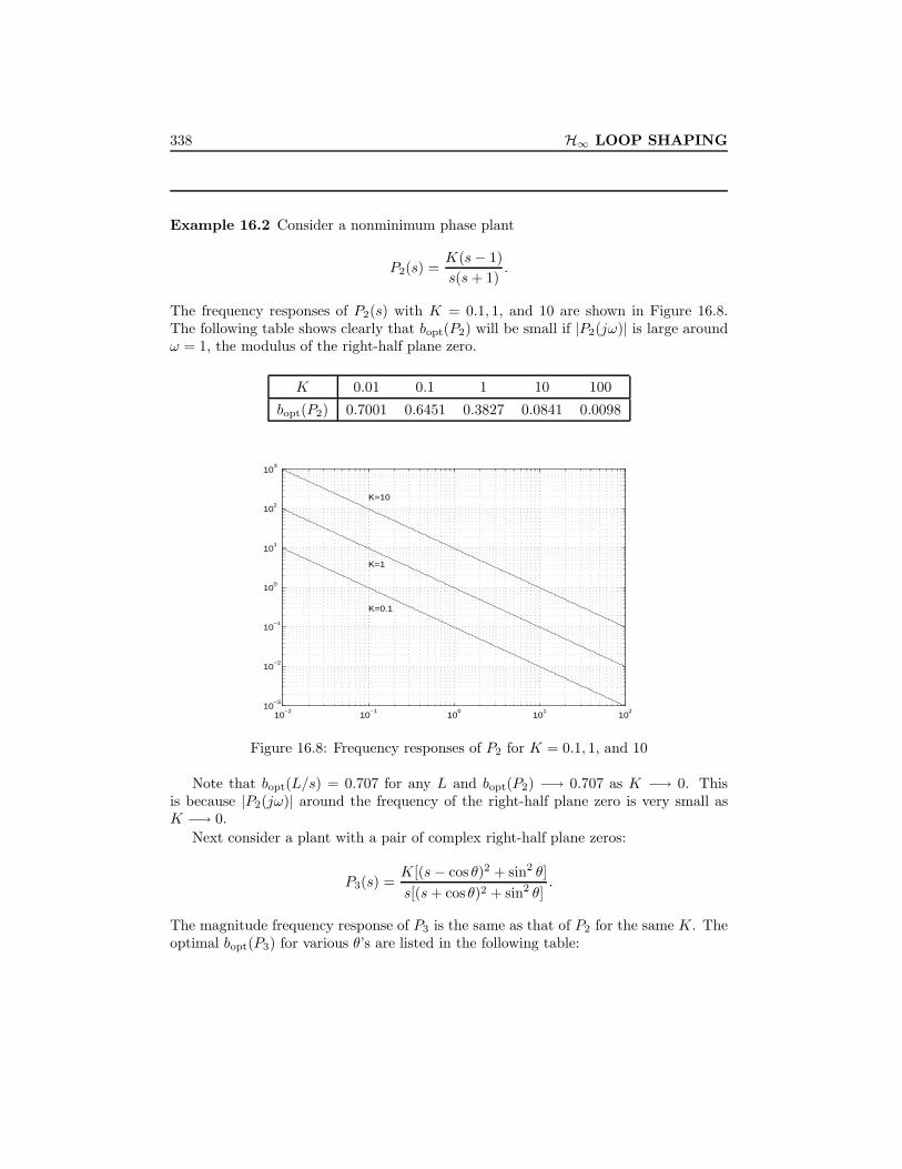
338 H∞ LOOP SHAPING
Example 16.2 Consider a nonminimum phase plant
P2(s) =K(s− 1)s(s+ 1)
.
The frequency responses of P2(s) with K = 0.1, 1, and 10 are shown in Figure 16.8.The following table shows clearly that bopt(P2) will be small if |P2(jω)| is large aroundω = 1, the modulus of the right-half plane zero.
K 0.01 0.1 1 10 100
bopt(P2) 0.7001 0.6451 0.3827 0.0841 0.0098
10−2
10−1
100
101
102
10−3
10−2
10−1
100
101
102
103
K=0.1
K=1
K=10
Figure 16.8: Frequency responses of P2 for K = 0.1, 1, and 10
Note that bopt(L/s) = 0.707 for any L and bopt(P2) −→ 0.707 as K −→ 0. Thisis because |P2(jω)| around the frequency of the right-half plane zero is very small asK −→ 0.
Next consider a plant with a pair of complex right-half plane zeros:
P3(s) =K[(s− cos θ)2 + sin2 θ]s[(s+ cos θ)2 + sin2 θ]
.
The magnitude frequency response of P3 is the same as that of P2 for the same K. Theoptimal bopt(P3) for various θ’s are listed in the following table:

16.4. Further Guidelines for Loop Shaping 339
θ (degree) 0 45 60 80 85K = 0.1 bopt(P3) 0.5952 0.6230 0.6447 0.6835 0.6950
θ (degree) 0 45 60 80 85K = 1 bopt(P3) 0.2588 0.3078 0.3568 0.4881 0.5512
θ (degree) 0 45 60 80 85K = 10 bopt(P3) 0.0391 0.0488 0.0584 0.0813 0.0897
It can also be concluded from the table that bopt(P3) will be small if |P3(jω)| islarge around the frequency of ω = 1 (the modulus of the right-half plane zero). It canbe further concluded that, for zeros with the same modulus, bopt(P3) will be smallerfor a plant with relatively larger real part zeros than for a plant with relatively largerimaginary part zeros (i.e., a pair of real right-half plane zeros has a much worse effecton the performance than a pair of almost pure imaginary axis right-half plane zeros ofthe same modulus).
Example 16.3 Consider an unstable plant
P4(s) =K(s+ 1)s(s− 1)
.
The magnitude frequency response of P4 is again the same as that of P2 for the sameK. The following table shows that bopt(P4) will be small if |P4(jω)| is small aroundω = 1 (the modulus of the right-half plane pole).
K 0.01 0.1 1 10 100
bopt(P4) 0.0098 0.0841 0.3827 0.6451 0.7001
Note that bopt(P4) −→ 0.707 as K −→ ∞. This is because |P4(jω)| is very largearound the frequency of the modulus of the right-half plane pole as K −→∞.
Next consider a plant with complex right-half plane poles:
P5(s) =K[(s+ cos θ)2 + sin2 θ]s[(s− cos θ)2 + sin2 θ]
.
The optimal bopt(P5) for various θ’s are listed in the following table:

340 H∞ LOOP SHAPING
θ (degree) 0 45 60 80 85K = 0.1 bopt(P5) 0.0391 0.0488 0.0584 0.0813 0.0897
θ (degree) 0 45 60 80 85K = 1 bopt(P5) 0.2588 0.3078 0.3568 0.4881 0.5512
θ (degree) 0 45 60 80 85K = 10 bopt(P5) 0.5952 0.6230 0.6447 0.6835 0.6950
It can also be concluded from the table that bopt(P5) will be small if |P5(jω)| issmall around the frequency of the modulus of the right-half plane pole. It can befurther concluded that, for poles with the same modulus, bopt(P5) will be smaller fora plant with relatively larger real part poles than for a plant with relatively largerimaginary part poles (i.e., a pair of real right-half plane poles has a much worse effecton the performance than a pair of almost pure imaginary axis right-half plane poles ofthe same modulus).
Example 16.4 Let a stable and minimum phase transfer function be
P6(s) =K(0.2s+ 1)4
s(s+ 1)4.
10−3
10−2
10−1
100
101
102
103
10−15
10−10
10−5
100
105
1010
1015
K=0.00001
K=0.1
K=10000
Figure 16.9: Frequency response of P6 for K = 10−5, 10−1 and 104
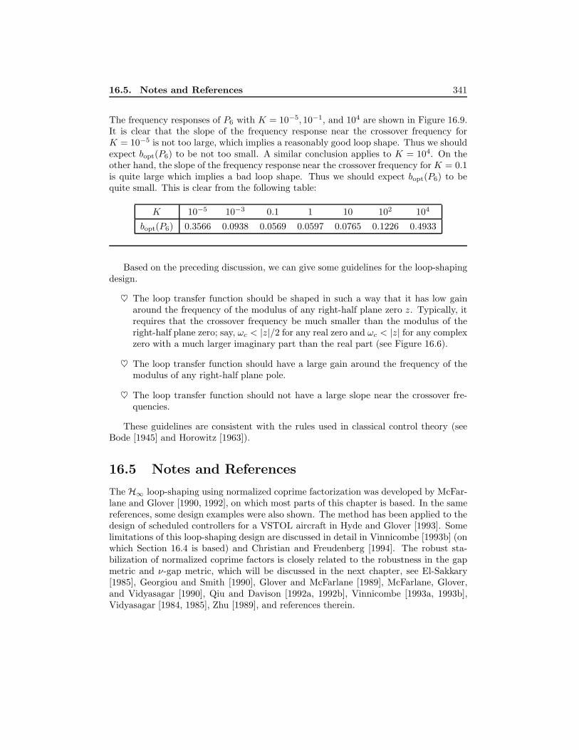
16.5. Notes and References 341
The frequency responses of P6 with K = 10−5, 10−1, and 104 are shown in Figure 16.9.It is clear that the slope of the frequency response near the crossover frequency forK = 10−5 is not too large, which implies a reasonably good loop shape. Thus we shouldexpect bopt(P6) to be not too small. A similar conclusion applies to K = 104. On theother hand, the slope of the frequency response near the crossover frequency for K = 0.1is quite large which implies a bad loop shape. Thus we should expect bopt(P6) to bequite small. This is clear from the following table:
K 10−5 10−3 0.1 1 10 102 104
bopt(P6) 0.3566 0.0938 0.0569 0.0597 0.0765 0.1226 0.4933
Based on the preceding discussion, we can give some guidelines for the loop-shapingdesign.
♥ The loop transfer function should be shaped in such a way that it has low gainaround the frequency of the modulus of any right-half plane zero z. Typically, itrequires that the crossover frequency be much smaller than the modulus of theright-half plane zero; say, ωc < |z|/2 for any real zero and ωc < |z| for any complexzero with a much larger imaginary part than the real part (see Figure 16.6).
♥ The loop transfer function should have a large gain around the frequency of themodulus of any right-half plane pole.
♥ The loop transfer function should not have a large slope near the crossover fre-quencies.
These guidelines are consistent with the rules used in classical control theory (seeBode [1945] and Horowitz [1963]).
16.5 Notes and References
The H∞ loop-shaping using normalized coprime factorization was developed by McFar-lane and Glover [1990, 1992], on which most parts of this chapter is based. In the samereferences, some design examples were also shown. The method has been applied to thedesign of scheduled controllers for a VSTOL aircraft in Hyde and Glover [1993]. Somelimitations of this loop-shaping design are discussed in detail in Vinnicombe [1993b] (onwhich Section 16.4 is based) and Christian and Freudenberg [1994]. The robust sta-bilization of normalized coprime factors is closely related to the robustness in the gapmetric and ν-gap metric, which will be discussed in the next chapter, see El-Sakkary[1985], Georgiou and Smith [1990], Glover and McFarlane [1989], McFarlane, Glover,and Vidyasagar [1990], Qiu and Davison [1992a, 1992b], Vinnicombe [1993a, 1993b],Vidyasagar [1984, 1985], Zhu [1989], and references therein.

342 H∞ LOOP SHAPING
16.6 Problems
Problem 16.1 Consider a feedback system with G(s) =1
s− 2. Compute by hand εmax,
the maximum stability radius for a normalized coprime factor perturbation of G(s).
Problem 16.2 In Corollary 16.2, find the parameterization of all H∞ controllers.
Problem 16.3 Let P∆ = (N + ∆N )(M + ∆M )−1 be a right coprime factor perturbedplant with a nominal plant P = NM−1, where (N,M) is a pair of normalized rightcoprime factorization. Formulate the corresponding robust stabilization problem asan H∞ control problem and find a stabilizing controller using the H∞ formulas inChapter 14. Are there any connections between this stabilizing controller and thecontroller obtained in this chapter for left coprime stabilization?
Problem 16.4 Let P have coprime factorizations P = NM−1 = M−1N . Then thereexist U, V, U , V ∈ H∞ such that[
M U
N V
][V −UN M
]= I.
Furthermore, all stabilizing controllers for P can be written as
K = (U +MQ)(V +NQ)−1, Q ∈ H∞.
Show that [K
I
](I + PK)−1M−1 =
[U +MQ
V +NQ
].
Suppose P = NM−1 = M−1N are normalized coprime factorizations. Show that
b−1P,K =
∥∥∥∥∥[U
V
]+
[M
N
]Q
∥∥∥∥∥∞
=
∥∥∥∥∥[R+Q
I
]∥∥∥∥∥∞
where R = M∼U +N∼V .
Problem 16.5 Let K be a controller that stabilizes the plant P . Show that
1. K stabilizes P = P + ∆a such that ∆a ∈ H∞ and ‖∆a‖ < bP,K ;
2. K stabilizes P = P (I + ∆m) such that ∆m ∈ H∞ and ‖∆m‖ < bP,K ;
3. K stabilizes P = (I + ∆m)P such that ∆m ∈ H∞ and ‖∆m‖ < bP,K ;
4. K stabilizes P = P (I + ∆f )−1 such that ∆f ∈ H∞ and ‖∆f‖ < bP,K ;
5. K stabilizes P = (I + ∆f )−1P such that ∆f ∈ H∞ and ‖∆f‖ < bP,K .
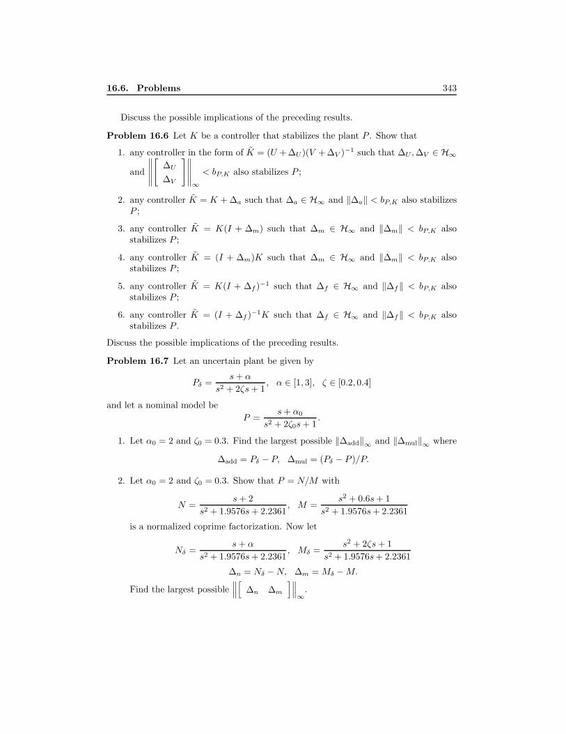
16.6. Problems 343
Discuss the possible implications of the preceding results.
Problem 16.6 Let K be a controller that stabilizes the plant P . Show that
1. any controller in the form of K = (U + ∆U )(V + ∆V )−1 such that ∆U ,∆V ∈ H∞
and
∥∥∥∥∥[
∆U
∆V
]∥∥∥∥∥∞
< bP,K also stabilizes P ;
2. any controller K = K + ∆a such that ∆a ∈ H∞ and ‖∆a‖ < bP,K also stabilizesP ;
3. any controller K = K(I + ∆m) such that ∆m ∈ H∞ and ‖∆m‖ < bP,K alsostabilizes P ;
4. any controller K = (I + ∆m)K such that ∆m ∈ H∞ and ‖∆m‖ < bP,K alsostabilizes P ;
5. any controller K = K(I + ∆f )−1 such that ∆f ∈ H∞ and ‖∆f‖ < bP,K alsostabilizes P ;
6. any controller K = (I + ∆f )−1K such that ∆f ∈ H∞ and ‖∆f‖ < bP,K alsostabilizes P .
Discuss the possible implications of the preceding results.
Problem 16.7 Let an uncertain plant be given by
Pδ =s+ α
s2 + 2ζs+ 1, α ∈ [1, 3], ζ ∈ [0.2, 0.4]
and let a nominal model beP =
s+ α0
s2 + 2ζ0s+ 1.
1. Let α0 = 2 and ζ0 = 0.3. Find the largest possible ‖∆add‖∞ and ‖∆mul‖∞ where
∆add = Pδ − P, ∆mul = (Pδ − P )/P.
2. Let α0 = 2 and ζ0 = 0.3. Show that P = N/M with
N =s+ 2
s2 + 1.9576s+ 2.2361, M =
s2 + 0.6s+ 1s2 + 1.9576s+ 2.2361
is a normalized coprime factorization. Now let
Nδ =s+ α
s2 + 1.9576s+ 2.2361, Mδ =
s2 + 2ζs+ 1s2 + 1.9576s+ 2.2361
∆n = Nδ −N, ∆m = Mδ −M.
Find the largest possible∥∥∥[ ∆n ∆m
]∥∥∥∞
.

344 H∞ LOOP SHAPING
3. In part 2, let (Nδ,Mδ) be a normalized coprime factorization of Pδ. Find thelargest possible
∥∥∥[ ∆n ∆m
]∥∥∥∞
.
4. Find the optimal nominal α0 and ζ0 such that the largest possible ‖∆add‖∞,
‖∆mul‖∞, and∥∥∥[ ∆n ∆m
]∥∥∥∞
are minimized, respectively.
Discuss the advantages of each uncertainty modeling method in terms of robust stabi-lizations.
Problem 16.8 Let P =−10
s(s− 1). Design (a) a precompensator W of order no greater
than 2 such that the crossover frequency ωc ≤ 2 and bopt(WP ) is as large as possible;(b) find the optimal loop-shaping controller K = K∞W with the W obtained in part(a).
Problem 16.9 Let P =100(1− s)s(s+ 10)
. Design (a) a precompensator W of order no
greater than 2 such that the crossover frequency ωc ≥ 1 and bopt(WP ) is as large aspossible; (b) find the optimal loop-shaping controller K = K∞W with the W obtainedin part (a).
Problem 16.10 Let G(s) =
[A B
C 0
]and G(s) = NM−1 with
[N
M
]=
A+BF B
C 0F I
where F is chosen such that NM−1 is a normalized right coprime factorization. Let[N
M
]be an rth order balanced truncation of
[N
M
]. Show that
[N
M
]is also a
normalized right coprime factorization.
Problem 16.11 (Reduced-Order Controllers by Controller Model Reduction; see Mc-
Farlane and Glover [1990], Zhou and Chen [1995].) Let G(s) =
[A B
C 0
]= M−1N
be a normalized left coprime factorization and let K(s) be a suboptimal controller givenin Corollary 18.2 (with performance γ). Let K = UV −1 be a right coprime factorization
[U
V
]=
A−BB∗X∞ −Y C∗
−C I
−B∗X∞ 0

16.6. Problems 345
and U , V ∈ RH∞ be approximations of U and V . Define
ε :=
∥∥∥∥∥[U
V
]−[U
V
]∥∥∥∥∥∞
and Kr = U V −1. Show that Kr is a stabilizing controller for G if ε < 1 and∥∥∥∥∥[Kr
I
](I +GKr)−1M−1
∥∥∥∥∥∞
=
∥∥∥∥∥[Kr
I
](I +GKr)−1
[I G
]∥∥∥∥∥∞
<γ
1− ε .
Problem 16.12 (Reduced Order Controllers by Plant Model Reduction; see McFarlaneand Glover [1990].) Let G = M−1N be a normalized left coprime factorization and letK be a stabilizing controller such that∥∥∥∥∥
[K
I
](I +GK)−1M−1
∥∥∥∥∥∞
≤ δ−1.
Let Gr := M−1r Nr be an approximation of G and
ε :=∥∥∥[ M − Mr N − Nr
]∥∥∥∞< δ.
(a) Show that K stabilizes Gr and∥∥∥∥∥[K
I
](I +GrK)−1M−1
r
∥∥∥∥∥∞
≤ (δ − ε)−1.
(b) Let W (s),W−1(s) ∈ RH∞ be obtained from the following spectral factorization:
W−1W−∗ = MrM∗r + NrN
∗r .
Show that ‖W‖∞ ≤1
1− ε and∥∥W−1
∥∥∞ ≤ 1 + ε.
(c) Show that
δ−1rn := inf
K1
∥∥∥∥∥[K1
I
](I +GrK1)−1(WMr)−1
∥∥∥∥∥∞
= infK1
∥∥∥∥∥[K1
I
](I +GrK1)−1
[I Gr
]∥∥∥∥∥∞
≤∥∥W−1
∥∥∞
δ − ε ≤ 1 + ε
δ − ε .
and ∥∥∥∥∥[K1
I
](I +GrK1)−1M−1
r
∥∥∥∥∥∞
≤ δ−1rn ‖W‖∞ .

346 H∞ LOOP SHAPING
(d) With the controller K1 given in (c), show that∥∥∥∥∥[K1
I
](I +GK1)−1M−1
∥∥∥∥∥∞
=
∥∥∥∥∥[K1
I
](I +GK1)−1
[I G
]∥∥∥∥∥∞
≤ δ−1red
where
δred :=δrn‖W‖∞
− ε ≤ δ − ε‖W−1‖∞ ‖W‖∞
− ε ≤ 1− ε1 + ε
(δ − ε)− ε.
Note that if Nr and Mr are the kth-order balanced truncation of N and M , thenδ = δrn =
√1− σ2
1 , δred = δ − ε, and ε ≤ 2∑ni=k+1 σi, where σi are the Hankel
singular values of[M N
].
(e) Show that
δ−1r := inf
K2
∥∥∥∥∥[K2
I
](I +GrK2)−1M−1
r
∥∥∥∥∥∞
≤ (δ − ε)−1.
(f) With the controller K2 given in (e), show that∥∥∥∥∥[K2
I
](I +GK2)−1M−1
∥∥∥∥∥∞
=
∥∥∥∥∥[K2
I
](I +GK2)−1
[I G
]∥∥∥∥∥∞
≤ (δr − ε)−1 ≤ (δ − 2ε)−1.
Again note that if Nr and Mr are the kth-order balanced truncation of N and M ,then δr = δ.
(Note that K1 and K2 are reduced-order controllers.)
Problem 16.13 Let G(s) =
[A B
C 0
]= M−1N be a normalized left coprime factor-
ization and let K(s) be a suboptimal controller given in Corollary 18.2 (with perfor-mance γ):
K(s) =
[A−BB∗X∞ − Y C∗C −Y C∗
−B∗X∞ 0
]where
X∞ =γ2
γ2 − 1Q
(I − γ2
γ2 − 1Y Q
)−1
andAY + Y A∗ − Y C∗CY +BB∗ = 0

16.6. Problems 347
Q(A− Y C∗C) + (A− Y C∗C)∗Q+ C∗C = 0.
Suppose Y and Q are balanced; that is,
Y = Q = diag(σ1, . . . , σr, σr+1, . . . , σn) = diag(Σ1,Σ2)
and let G(s) be partitioned accordingly as
G(s) =
A11 A12 B1
A21 A22 B2
C1 C2 0
.Denote Y1 = Σ1 and X1 = γ2
γ2−1Σ1
(I − γ2
γ2−1Σ21
)−1
. Show that
Kr(s) =
[A11 −B1B
∗1X1 − Y1C
∗1C1 −Y1C
∗1
−B∗1X1 0
]
is exactly the reduced-order controller obtained from the last problem with balancedmodel reduction procedure. (It is also interesting to note that
Q = X(I + Y X)−1
where X = X∗ ≥ 0 is the stabilizing solution to
XA+A∗X −XBB∗X + C∗C = 0.
Hence balancing Y and Q is equivalent to balancing X and Y . This is called Riccatibalancing; see Jonckheere and Silverman [1983].)
Problem 16.14 Apply the controller reduction methods in the last three problems,
respectively, to a satellite system G(s) =
[A B
C 0
]where
A =
0 1 0 00 0 0 00 0 0 10 0 −1.5392 −2× 0.003× 1.539
, B =
0
1.7319× 10⁻⁵
03.7859× 10⁻⁴
,
C =[
1 0 1 0], D = 0.
Compare the results (see McFarlane and Glover [1990] for further details).

348 H∞ LOOP SHAPING
Problem 16.15 Let f(s) be analytic in the closed right-half plane and suppose
limr→∞
maxθ∈[−π/2,π/2]
|f(rejθ)r
= 0.
Then the Poisson integral formula (see, for example, Freudenberg and Looze [1988],page 37) says that f(s) at any point s = x + jy in the open right-half plane can berecovered from f(jω) via the integral relation:
f(s) =1π
∫ ∞−∞
f(jω)x
x2 + (y − ω)2dω.
Let s = rejθ (i.e., x = r cos θ and y = r sin θ) with r > 0 and −π/2 < θ < π/2. Supposef(jω) = f(−jω). Show that
f(rejθ) =∫ ∞−∞
f(jω)Kθ(ω/r) d(lnω)
where
Kθ(ω/r) =1π
2(ω/r)[1 + (ω/r)2] cos θ[1− (ω/r)2]2 + 4(ω/r)2 cos2 θ

Chapter 17
Gap Metric and ν-Gap Metric
In the previous chapters, we have seen that all of robust control design techniques assumethat we have some description of the model uncertainties (i.e., we have a measure ofthe distance from the nominal plant to the set of uncertainty systems). This measureis usually chosen to be a metric or a norm. However, the operator norm can be a poormeasure of the distance between systems in respect to feedback control system design.For example, consider
P1(s) =1s, P2(s) =
1s+ 0.1
.
The closed-loop complementary sensitivity functions corresponding to P1 and P2 withunity feedback are relatively close and their difference is∥∥P1(I + P1)−1 − P2(I + P2)−1
∥∥∞ = 0.0909,
but the difference between P1 and P2 is
‖P1 − P2‖∞ =∞.
This shows that the closed-loop behavior of two systems can be very close even thoughthe norm of the difference between the two open-loop systems can be arbitrarily large.
To deal with such problems, the gap metric and the ν-gap metric were introducedinto the control literature by Zames and El-Sakkary [1980] (see also El-Sakkary [1985]and Vinnicombe [1993]) as being appropriate for the study of uncertainty in feedbacksystems. An alternative metric, the graph metric, was also introduced by Vidyasagar[1984] in terms of normalized coprime factorizations. All of these metrics are equivalent,and thus induce the same topology. This topology is the weakest in which feedbackstability is a robust property. The metrics define notions of distance in the space of(possible) unstable systems that do not assume that the plants have the same numberof poles in the right-half plane.
We shall briefly introduce the gap metric in Section 17.1 and study some of itsapplications in robust control. Our focus in this chapter is Sections 17.2–17.4, which
349

350 GAP METRIC AND ν-GAP METRIC
study in some detail the ν-gap metric. In particular, we introduce the ν-gap metricin Section 17.2 and explore its frequency domain interpretation and applications inSection 17.3 and Section 17.4. Finally, we consider controller order reduction in the gapor ν-gap metric framework in Section 17.5.
17.1 Gap Metric
In this section we briefly introduce the gap metric and discuss some of its applicationsin controller design.
Let P (s) be a p×m rational transfer matrix and let P have the following normalizedright and left stable coprime factorizations:
P = NM−1 = M−1N .
That is,M∼M +N∼N = I, MM∼ + NN∼ = I.
The graph of the operator P is the subspace of H2 consisting of all pairs (u, y) suchthat y = Pu. This is given by [
M
N
]H2
and is a closed subspace of H2. The gap between two systems P1 and P2 is defined by
δg(P1, P2) =
∥∥∥∥∥∥∥∥∥Π[M1
N1
]H2
−Π[M2
N2
]H2
∥∥∥∥∥∥∥∥∥where ΠK denotes the orthogonal projection onto K and P1 = N1M
−11 and P2 =
N2M−12 are normalized right coprime factorizations.
It is shown by Georgiou [1988] that the gap metric can be computed as follows:
Theorem 17.1 Let P1 = N1M−11 and P2 = N2M
−12 be normalized right coprime fac-
torizations. Thenδg(P1, P2) = max
~δ(P1, P2), ~δ(P2, P1)
where ~δg(P1, P2) is the directed gap and can be computed by
~δg(P1, P2) = infQ∈H∞
∥∥∥∥∥[M1
N1
]−[M2
N2
]Q
∥∥∥∥∥∞
.
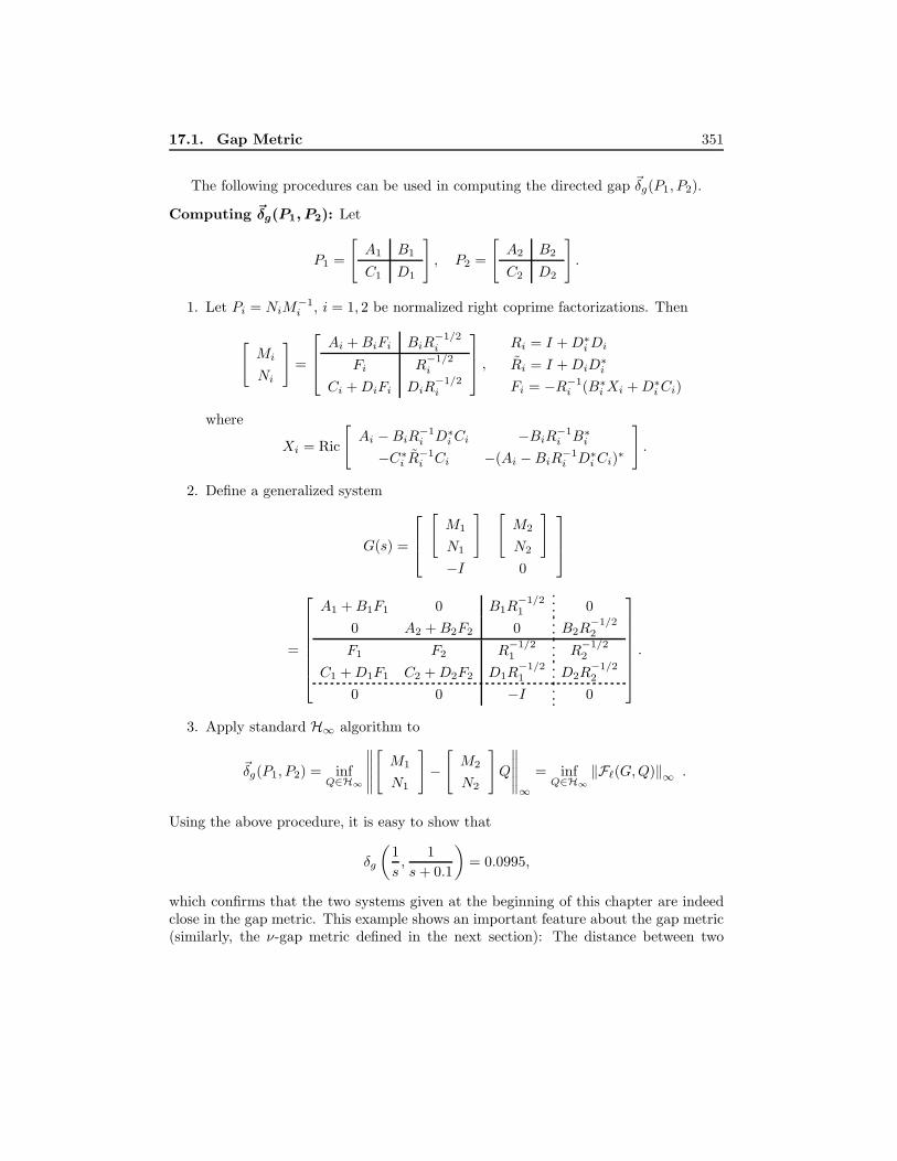
17.1. Gap Metric 351
The following procedures can be used in computing the directed gap ~δg(P1, P2).
Computing ~δg(P1, P2): Let
P1 =
[A1 B1
C1 D1
], P2 =
[A2 B2
C2 D2
].
1. Let Pi = NiM−1i , i = 1, 2 be normalized right coprime factorizations. Then
[Mi
Ni
]=
Ai +BiFi BiR−1/2i
Fi R−1/2i
Ci +DiFi DiR−1/2i
, Ri = I +D∗iDi
Ri = I +DiD∗i
Fi = −R−1i (B∗iXi +D∗iCi)
where
Xi = Ric
[Ai −BiR−1
i D∗iCi −BiR−1i B∗i
−C∗i R−1i Ci −(Ai −BiR−1
i D∗iCi)∗
].
2. Define a generalized system
G(s) =
[M1
N1
] [M2
N2
]−I 0
=
A1 +B1F1 0 B1R
−1/21 0
0 A2 +B2F2 0 B2R−1/22
F1 F2 R−1/21 R
−1/22
C1 +D1F1 C2 +D2F2 D1R−1/21 D2R
−1/22
0 0 −I 0
.
3. Apply standard H∞ algorithm to
~δg(P1, P2) = infQ∈H∞
∥∥∥∥∥[M1
N1
]−[M2
N2
]Q
∥∥∥∥∥∞
= infQ∈H∞
‖F`(G,Q)‖∞ .
Using the above procedure, it is easy to show that
δg
(1s,
1s+ 0.1
)= 0.0995,
which confirms that the two systems given at the beginning of this chapter are indeedclose in the gap metric. This example shows an important feature about the gap metric(similarly, the ν-gap metric defined in the next section): The distance between two

352 GAP METRIC AND ν-GAP METRIC
plants, as measured by the gap metric δg (or the ν-gap metric δν), has very little to dowith any difference between their open-loop behavior (indeed, there is no reason why itshould). This point will be further illustrated by an example in the next section.
A lower bound for the gap metric can also be obtained easily without actually solvingthe corresponding H∞ optimization. Let
Φ =
[M∼2 N∼2−N2 M2
].
Then Φ∼Φ = ΦΦ∼ = I and
~δg(P1, P2) = infQ∈H∞
∥∥∥∥∥[M∼2 N∼2−N2 M2
][M1
N1
]−[M2
N2
]Q
∥∥∥∥∥∞
= infQ∈H∞
∥∥∥∥∥[M∼2 M1 +N∼2 N1 −Q−N2M1 + M2N1
]∥∥∥∥∥∞
≥ ‖Ψ(P1, P2)‖∞
where
Ψ(P1, P2) := −N2M1 + M2N1 =[M2 N2
] [ 0 I
−I 0
][M1
N1
]. (17.1)
It will be seen in the next section that ‖Ψ(P1, P2)‖∞ is related to the ν-gap metric. Theabove lower bound may actually be achieved. Consider, for example,
P1 =k1
s+ 1, P2 =
k2
s+ 1.
Then it is easy to verify that Pi = Ni/Mi, i = 1, 2, with
Ni =ki
s+√
1 + k2i
, Mi =s+ 1
s+√
1 + k2i
,
are normalized coprime factorizations and it can be further shown, as in Georgiou andSmith [1990], that
δg(P1, P2) = ‖Ψ(P1, P2)‖∞ =
|k1 − k2||k1|+ |k2|
, if |k1k2| > 1;
|k1 − k2|√(1 + k2
1)(1 + k22), if |k1k2| ≤ 1.
An immediate consequence of Theorem 17.1 is the connection between the uncer-tainties in the gap metric and the uncertainties characterized by the normalized coprimefactors. The following corollary states that a ball of uncertainty in the directed gap isequivalent to a ball of uncertainty in the normalized coprime factors.

17.1. Gap Metric 353
Corollary 17.2 Let P have a normalized coprime factorization P = NM−1. Then forall 0 < b ≤ 1,
P1 : ~δg(P, P1) < b
=
P1 : P1 = (N + ∆N )(M + ∆M )−1, ∆N , ∆M ∈ H∞,
∥∥∥∥∥[
∆N
∆M
]∥∥∥∥∥∞
< b
.
Proof. Suppose ~δg(P, P1) < b and let P1 = N1M−11 be a normalized right coprime
factorization. Then there exists a Q ∈ H∞ such that∥∥∥∥∥[M
N
]−[M1
N1
]Q
∥∥∥∥∥∞
< b.
Define [∆M
∆N
]:=
[M1
N1
]Q−
[M
N
]∈ H∞.
Then
∥∥∥∥∥[
∆M
∆N
]∥∥∥∥∥∞
< b and P1 = (N1Q)(M1Q)−1 = (N + ∆N )(M + ∆M )−1.
To show the converse, note that P1 = (N + ∆N )(M + ∆M )−1 and there exists a
Q−1 ∈ H∞ such that P1 =
(N + ∆N )Q
(M + ∆M )Q−1
is a normalized right
coprime factorization. Hence by definition, ~δg(P, P1) can be computed as
~δg(P, P1) = infQ
∥∥∥∥∥[M
N
]−[M + ∆M
N + ∆N
∥∥∥∥∥∞
≤∥∥∥∥∥[M
N
]−[M + ∆M
N + ∆N
]∥∥∥∥∥∞
< b
where the first inequality follows by taking Q = Q−1 ∈ H∞. 2
The following is a list of useful properties of the gap metric shown by Georgiou andSmith [1990].
• If δg(P1, P2) < 1, then δg(P1, P2) = ~δg(P1, P2) = ~δg(P2, P1).
• If b ≤ λ(P ) := infRes>0
σ
([M(s)N(s)
]), then
P1 : ~δ(P, P1) < b
= P1 : δ(P, P1) < b .

354 GAP METRIC AND ν-GAP METRIC
Recall that
bobt(P ) :=
inf
K stabilizing
∥∥∥∥∥[I
K
](I + PK)−1
[I P
]∥∥∥∥∥∞
−1
=√
1− λmax(Y Q) =
√1−
∥∥∥[ N M]∥∥∥2
H
and
bP,K :=
∥∥∥∥∥[I
K
](I + PK)−1
[I P
]∥∥∥∥∥−1
∞
=
∥∥∥∥∥[I
P
](I +KP )−1
[I K
]∥∥∥∥∥−1
∞
.
The following results were shown by Qiu and Davison [1992a].
Theorem 17.3 Suppose the feedback system with the pair (P0,K0) is stable. Let P :=P : δg(P, P0) < r1 and K := K : δg(K,K0) < r2. Then
(a) The feedback system with the pair (P,K) is also stable for all P ∈ P and K ∈ Kif and only if
arcsin bP0,K0 ≥ arcsin r1 + arcsin r2.
(b) The worst possible performance resulting from these sets of plants and controllersis given by
infP∈P, K∈K
arcsin bP,K = arcsin bP0,K0 − arcsin r1 − arcsin r2.
The sufficiency part of the theorem follows from Theorem 17.8 in the next section. Notethat the theorem is still true if one of the uncertainty balls is taken as closed ball. Inparticular, one can take either r1 = 0 or r2 = 0.
Example 17.1 Consider
P1 =s− 1s+ 1
, P2 =2s− 1s+ 1
.
Then P1 = N1/M1 and P2 = N2/M2 with
N1 =1√2s− 1s+ 1
, M1 =1√2, N2 =
2s− 1√5s+
√2, M2 =
s+ 1√5s+
√2
are normalized coprime factorizations. It is easy to show that
δg(P1, P2) = 1/3 > ‖Ψ(P1, P2)‖∞ = supω
|ω|√10ω2 + 4
=1√10,

17.1. Gap Metric 355
which implies that any controller K that stabilizes P1 and achieves only bP1,K > 1/3will actually stabilize P2 by Theorem 17.3. The following Matlab command can beused to compute the gap:
δg(P1,P2) = gap(P1,P2, tol)
Next, note that bobt(P1) = 1/√
2 and the optimal controller achieving bobt(P1) is Kobt =0. There must be a plant P with δν(P1, P ) = bobt(P1) = 1/
√2 that can not be stabilized
byKobt = 0; that is, there must be an unstable plant P such that δν(P1, P ) = bobt(P1) =1/√
2. A such P can be found using Corollary 17.2:
P : δg(P1, P ) ≤ bobt(P1)
=
P : P =
N1 + ∆N
M1 + ∆M, ∆N , ∆M ∈ H∞,
∥∥∥∥∥[
∆N
∆M
]∥∥∥∥∥∞
≤ bobt(P1)
.
that is, there must be ∆N , ∆M ∈ H∞,∥∥∥∥∥[
∆N
∆M
]∥∥∥∥∥∞
= bobt(P1) such that
P =N1 + ∆N
M1 + ∆M
is unstable. Let∆N = 0, ∆M =
1√2s− 1s+ 1
.
ThenP =
N1 + ∆N
M1 + ∆M=s− 1
2s, δν(P1, P ) = bobt(P1) = 1/
√2.
Example 17.2 We shall now consider the following question: Given an uncertain plant
P (s) =k
s− 1, k ∈ [k1, k2],
(a) Find the best nominal design model P0 =k0
s− 1in the sense
infk0∈[k1,k2]
supk∈[k1,k2]
δg(P, P0).
(b) Let k1 be fixed and k2 be variable. Find the k0 so that the largest family of theplant P can be guaranteed to be stabilized a priori by any controller satisfyingbP0,K = bobt(P0).
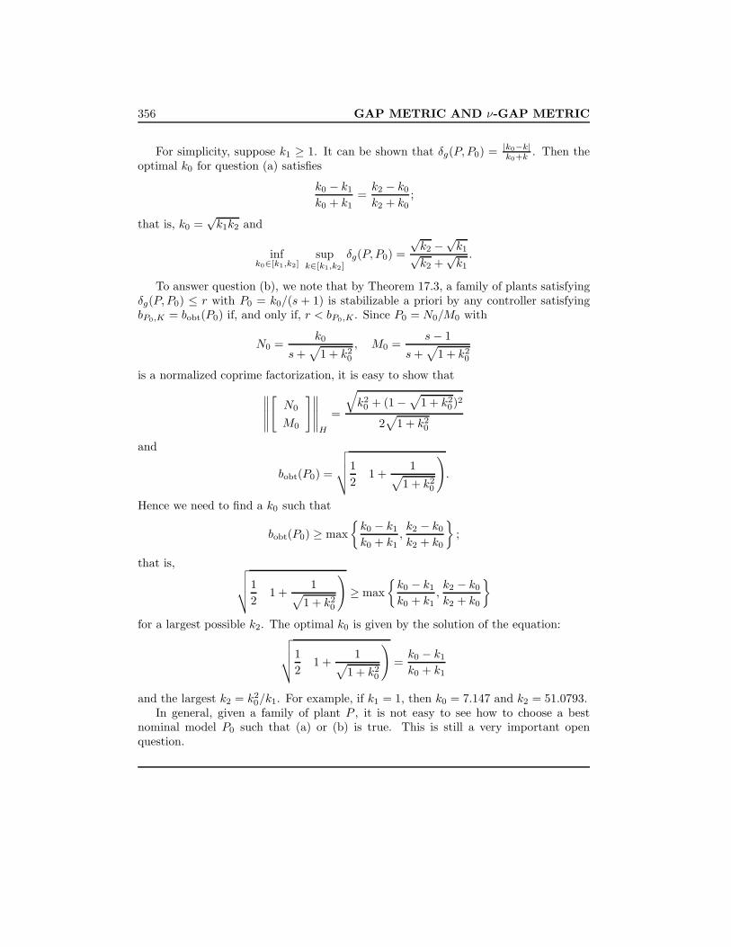
356 GAP METRIC AND ν-GAP METRIC
For simplicity, suppose k1 ≥ 1. It can be shown that δg(P, P0) = |k0−k|k0+k . Then the
optimal k0 for question (a) satisfies
k0 − k1
k0 + k1=k2 − k0
k2 + k0;
that is, k0 =√k1k2 and
infk0∈[k1,k2]
supk∈[k1,k2]
δg(P, P0) =√k2 −
√k1√
k2 +√k1
.
To answer question (b), we note that by Theorem 17.3, a family of plants satisfyingδg(P, P0) ≤ r with P0 = k0/(s + 1) is stabilizable a priori by any controller satisfyingbP0,K = bobt(P0) if, and only if, r < bP0,K . Since P0 = N0/M0 with
N0 =k0
s+√
1 + k20
, M0 =s− 1
s+√
1 + k20
is a normalized coprime factorization, it is easy to show that∥∥∥∥∥[N0
M0
]∥∥∥∥∥H
=
√k2
0 + (1−√
1 + k20)2
2√
1 + k20
and
bobt(P0) =
√√√√12
(1 +
1√1 + k2
0
).
Hence we need to find a k0 such that
bobt(P0) ≥ maxk0 − k1
k0 + k1,k2 − k0
k2 + k0
;
that is, √√√√12
(1 +
1√1 + k2
0
)≥ max
k0 − k1
k0 + k1,k2 − k0
k2 + k0
for a largest possible k2. The optimal k0 is given by the solution of the equation:√√√√1
2
(1 +
1√1 + k2
0
)=k0 − k1
k0 + k1
and the largest k2 = k20/k1. For example, if k1 = 1, then k0 = 7.147 and k2 = 51.0793.
In general, given a family of plant P , it is not easy to see how to choose a bestnominal model P0 such that (a) or (b) is true. This is still a very important openquestion.

17.2. ν-Gap Metric 357
17.2 ν-Gap Metric
The shortfall of the gap metric is that it is not easily related to the frequency responseof the system. On the other hand, the ν-gap metric to be introduced in this sectionhas a clear frequency domain interpolation and can, in general, be computed fromfrequency response. The presentation given in this section, Sections 17.3, 17.4, and17.5 are based on Vinnicombe [1993a, 1993b], to which readers are referred for furtherdetailed discussions.
To define the new metric, we shall first review a basic concept from the complexanalysis.
Definition 17.1 Let g(s) be a scalar transfer function and let Γ denote a Nyquistcontour indented around the right of any imaginary axis poles of g(s), as shown inFigure 17.1. Then the winding number of g(s) with respect to this contour, denotedby wno(g), is the number of counterclockwise encirclements around the origin by g(s)evaluated on the Nyquist contour Γ. (A clockwise encirclement counts as a negativeencirclement.)
Γ
0
Figure 17.1: The Nyquist contour
The following argument principle is standard and can be found from any complexanalysis book.
Lemma 17.4 (The Argument Principle) Let Γ be a closed contour in the complexplane. Let f(s) be a function analytic along the contour; that is, f(s) has no poles on Γ.Assume f(s) has Z zeros and P poles inside Γ. Then f(s) evaluated along the contourΓ once in an anticlockwise direction will make Z−P anticlockwise encirclements of theorigin.

358 GAP METRIC AND ν-GAP METRIC
Let G(s) be a matrix (or scalar) transfer matrix. We shall denote η(G) and η0(G),respectively, the number of open right-half plane and imaginary axis poles of G(s).
The winding number has the following properties:
Lemma 17.5 Let g and h be biproper rational scalar transfer functions and let F be asquare transfer matrix. Then
(a) wno(gh) = wno(g)+wno(h);
(b) wno(g) = η(g−1)− η(g);
(c) wno(g∼) = −wno(g)− η0(g−1) + η0(g);
(d) wno(1 + g) = 0 if g ∈ RL∞ and ‖g‖∞ < 1;
(e) wno det(I + F ) = 0 if F ∈ RL∞ and ‖F‖∞ < 1.
Proof. Part (a) is obvious by the argument principle. To show part (b), note that bythe argument principle wno(g) equals the excess of the number of open right-half planezeros of g over the number of open right-half plane poles of g; that is, wno(g) = η(g−1)−η(g), since the number of right-half plane zeros of g is the number of right-half planepoles of g−1. Next, suppose the order of g in part (c) is n. Then η(g∼) = n−η(g)−η0(g)and η
[(g∼)−1
]= n − η(g−1) − η0(g−1), which gives wno(g∼) = η
[(g∼)−1
]− η(g∼) =
η(g)− η(g−1)− η0(g−1) + η0(g) = −wno(g)− η0(g−1) + η0(g). Part (d) follows from thefact that 1 + Reg(jω) > 0, ∀ω since ‖g‖∞ < 1. Finally, part (e) follows from part (d)and det(I + F ) =
∏mi=1(1 + λi(F )) with |λi(F )| < 1. 2
Example 17.3 Let
g1 =1.2(s+ 3)s− 5
, g2 =s− 1s− 2
, g3 =2(s− 1)(s− 2)(s+ 3)(s+ 4)
, g4 =(s− 1)(s+ 3)(s− 2)(s− 4)
.
Figure 17.2 shows the functions, g1, g2, g3, and g4, evaluated on the Nyquist contour Γ.Clearly, we have
wno(g1) = −1, wno(g2) = 0, wno(g3) = 2, wno(g4) = −1
and they are consistent with the results computed from using Lemma 17.5.
The ν-gap metric introduced in Vinnicombe [1993a, 1993b] is defined as follows:

17.2. ν-Gap Metric 359
g1g2g3g4
−1 −0.5 0 0.5 1 1.5 2−2
−1.5
−1
−0.5
0
0.5
1
1.5
2
real
ima
gin
ary
Figure 17.2: g1, g2, g3, and g4 evaluated on Γ
Definition 17.2 The ν-gap metric is defined as
δν(P1, P2) =
‖Ψ(P1, P2)‖∞ , if det Θ(jω) 6= 0 ∀ω
and wno det Θ(s) = 0,
1, otherwise
where Θ(s) := N∼2 N1 +M∼2 M1 and Ψ(P1, P2) := −N2M1 + M2N1.
Note that it can be shown as in Vinnicombe [1993a] that
δν(P1, P2) = δν(P2, P1) = δν(PT1 , PT2 )
and δν is indeed a metric (a proof of this fact is quite complex).
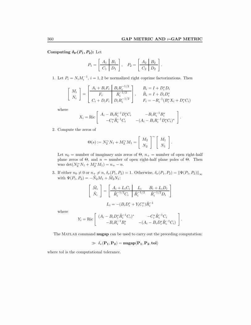
360 GAP METRIC AND ν-GAP METRIC
Computing δν(P1, P2): Let
P1 =
[A1 B1
C1 D1
], P2 =
[A2 B2
C2 D2
].
1. Let Pi = NiM−1i , i = 1, 2 be normalized right coprime factorizations. Then
[Mi
Ni
]=
Ai +BiFi BiR−1/2i
Fi R−1/2i
Ci +DiFi DiR−1/2i
, Ri = I +D∗iDi
Ri = I +DiD∗i
Fi = −R−1i (B∗iXi +D∗iCi)
where
Xi = Ric
[Ai −BiR−1
i D∗iCi −BiR−1i B∗i
−C∗i R−1i Ci −(Ai −BiR−1
i D∗iCi)∗
].
2. Compute the zeros of
Θ(s) := N∼2 N1 +M∼2 M1 =
[M2
N2
]∼ [M1
N1
].
Let n0 = number of imaginary axis zeros of Θ, n+ = number of open right-halfplane zeros of Θ, and n = number of open right-half plane poles of Θ. Thenwno det(N∼2 N1 +M∼2 M1) = n+ − n.
3. If either n0 6= 0 or n+ 6= n, δν(P1, P2) = 1. Otherwise, δν(P1, P2) = ‖Ψ(P1, P2)‖∞with Ψ(P1, P2) = −N2M1 + M2N1:[
Mi
Ni
]=
[Ai + LiCi Li Bi + LiDi
R−1/2i Ci R
−1/2i R
−1/2i Di
]
Li = −(BiD∗i + YiC∗i )R−1
i
where
Yi = Ric
[(Ai −BiD∗i R−1
i Ci)∗ −C∗i R−1i Ci
−BiR−1i B∗i −(Ai −BiD∗i R−1
i Ci)
].
The Matlab command nugap can be used to carry out the preceding computation:
δν(P1,P2) = nugap(P1,P2, tol)
where tol is the computational tolerance.

17.2. ν-Gap Metric 361
Example 17.4 Consider, for example, P1 = 1 and P2 =1s
. Then
M1 = N1 =1√2, M2 =
s
s+ 1, N2 =
1s+ 1
.
HenceΘ(s) =
1√2
1− s1− s =
1√2, Ψ(P1, P2) =
1√2s− 1s+ 1
,
and δν(P1, P2) = 1√2. (Note that Θ has no poles or zeros!)
The ν-gap metric can also be computed directly from the system transfer matriceswithout first finding the normalized coprime factorizations.
Theorem 17.6 The ν-gap metric can be defined as
δν(P1, P2) =
‖Ψ(P1, P2)‖∞ , if det(I + P∼2 P1) 6= 0 ∀ω and
wno det(I + P∼2 P1) + η(P1)− η(P2)− η0(P2) = 0,
1, otherwise
where Ψ(P1, P2) can be written as
Ψ(P1, P2) = (I + P2P∼2 )−1/2(P1 − P2)(I + P∼1 P1)−1/2.
Proof. Since the number of unstable zeros of M1 (M2) is equal to the number ofunstable poles of P1 (P2), and
N∼2 N1 +M∼2 M1 = M∼2 (I + P∼2 P1)M1,
we havewno det(N∼2 N1 +M∼2 M1) = wno det M∼2 (I + P∼2 P1)M1
= wno detM∼2 + wno det(I + P∼2 P1) + wno detM1.
Note that wno detM1 = η(P1), wno detM∼2 = −wno detM2 − η0(M−12 ) = −η(P2) −
η0(P2), and
wno det(N∼2 N1 +M∼2 M1) = −η(P2)− η0(P2) + wno det(I + P∼2 P1) + η(P1).
Furthermore,
det(N∼2 N1 +M∼2 M1) 6= 0, ∀ω ⇐⇒ det(I + P∼2 P1) 6= 0, ∀ω.

362 GAP METRIC AND ν-GAP METRIC
The theorem follows by noting that
Ψ(P1, P2) = (I + P2P∼2 )−1/2(P1 − P2)(I + P∼1 P1)−1/2
since Ψ(P1, P2) = −N2M1 + M2N1 = M2(P1 − P2)M1 and
M∼2 M2 = (I + P2P∼2 )−1, M1M
∼1 = (I + P∼1 P1)−1.
2
This alternative formula is useful when doing the hand calculation or when com-puting from the frequency response of the plants since it does not need to compute thenormalized coprime factorizations.
Example 17.5 Consider two plants P1 = 1 and P2 = 1/s. Then wno det(1 +P∼2 P1) =wno[(s− 1)/s] = 1, as shown in Figure 17.3(a), and wno det(1 + P∼2 P1) + η(P1) −η(P2) − η0(P2) = 0. On the other hand, wno det(1 + P∼1 P2) + η(P2) − η(P1) = wno(s+ 1)/s = 0, as shown in Figure 17.3(b).
(s−1)/s
−10 −5 0
−10
−5
0
5
10
(a)
(s+1)/s
0 5 10
−10
−5
0
5
10
(b)
Figure 17.3:s− 1s
ands+ 1s
evaluated on Γ
Similar to the gap metric, it is shown by Vinnicombe [1993a, 1993b] that the ν-gapmetric can also be characterized as an optimization problem (however, we shall not useit for computation).

17.2. ν-Gap Metric 363
Theorem 17.7 Let P1 = N1M−11 and P2 = N2M
−12 be normalized right coprime fac-
torizations. Then
δν(P1, P2) = infQ,Q−1 ∈ L∞
wno det(Q) = 0
∥∥∥∥∥[M1
N1
]−[M2
N2
]Q
∥∥∥∥∥∞
.
Moreover, δg(P1, P2)bobt(P1) ≤ δν(P1, P2) ≤ δg(P1, P2).
It is now easy to see thatP : δν(P0, P ) < r
⊃P = (N0 + ∆N )(M0 + ∆M )−1 :
[∆N
∆M
]∈ H∞,
∥∥∥∥∥[
∆N
∆M
]∥∥∥∥∥∞
< r
.
Define1
bP,K(ω):= σ
([I
K(jω)
](I + P (jω)K(jω))−1
[I P (jω)
])and
ψ(P1(jω), P2(jω)) = σ (Ψ(P1(jω), P2(jω))) .
The following theorem states that robust stability can be checked using the frequency-by-frequency test.
Theorem 17.8 Suppose (P0,K) is stable and δν(P0, P1) < 1. Then (P1,K) is stable if
bP0,K(ω) > ψ(P0(jω), P1(jω)), ∀ω.
Moreover,
arcsin bP1,K(ω) ≥ arcsin bP0,K(ω)− arcsinψ(P0(jω), P1(jω)), ∀ω
andarcsin bP1,K ≥ arcsin bP0,K − arcsin δν(P0, P1).
Proof. Let P1 = M−11 N1, P0 = N0M
−10 = M−1
0 N0 and K = UV −1 be normalizedcoprime factorizations, respectively. Then
1bP1,K(ω)
= σ
([V
U
](M1V + N1U)−1
[M1 N1
])= σ
((M1V + N1U)−1
).
That is,
bP1,K(ω) = σ(M1V + N1U) = σ
([M1 N1
] [ V
U
]).

364 GAP METRIC AND ν-GAP METRIC
Similarly,
bP0,K(ω) = σ(M0V + N0U) = σ
([M0 N0
] [ V
U
]).
Note that
ψ(P0(jω), P1(jω)) = σ
([M1 N1
] [ N0
−M0
])[
N0 M∼0−M0 N∼0
]∼ [N0 M∼0−M0 N∼0
]= I.
To simplify the derivation, define
G0 =
[N0
−M0
], G0 =
[M0 N0
], G1 =
[M1 N1
], F =
[V
U
].
Thenψ(P0, P1) = σ(G1G0), bP0,K(ω) = σ(G0F ), bP1,K(ω) = σ(G1F )
and [G0 G∼0
]∼ [G0 G∼0
]= I =⇒
[G0 G∼0
] [G0 G∼0
]∼= I.
That is,G0G
∼0 + G∼0 G0 = I.
Note that
I = G1G∼1 = G1(G0G
∼0 + G∼0 G0)G∼1 = (G1G0)(G1G0)∼ + (G1G
∼0 )(G1G
∼0 )∼.
Henceσ2(G1G
∼0 ) = 1− σ2(G1G0).
Similarly,
I = F∼F = F∼(G0G∼0 + G∼0 G0)F = (G∼0 F )∼(G∼0 F ) + (G0F )∼(G0F )
=⇒ σ2(G∼0 F ) = 1− σ2(G0F ).
By the assumption, ψ(P0, P1) < bP0,K(ω); that is,
σ(G1G0) < σ(G0F ), ∀ω
andσ(G∼0 F ) =
√1− σ2(G0F ) <
√1− σ2(G1G0) = σ(G1G
∼0 ).
Henceσ(G1G0)σ(G∼0 F ) < σ(G1G
∼0 )σ(G0F );

17.2. ν-Gap Metric 365
that is,σ(G1G0G
∼0 F ) < σ(G1G
∼0 G0F ), ∀ ω
=⇒∥∥∥(G1G
∼0 G0F )−1(G1G0G
∼0 F )
∥∥∥∞< 1.
NowG1F = G1(G∼0 G0 +G0G
∼0 )F = (G1G
∼0 G0F ) + (G1G0G
∼0 F )
= (G1G∼0 G0F )
(I + (G1G
∼0 G0F )−1(G1G0G
∼0 F )
).
By Lemma 17.5,
wno det(G1F ) = wno det(G1G∼0 G0F ) = wno det(G1G
∼0 ) + wno det(G0F ).
Since (P0,K) is stable =⇒ (G0F )−1 ∈ H∞ =⇒ η((G0F )−1) = 0
=⇒ wno det(G0F ) := η((G0F )−1)− η(G0F ) = 0.
Next, note thatPT0 = (NT
0 )(MT0 )−1, PT1 = (NT
1 )(MT1 )−1
and δν(PT0 , PT1 ) = δν(P0, P1) < 1; then, by definition of δν(PT0 , PT1 ),
wno det((NT0 )∼(NT
1 ) + (MT0 )∼(MT
1 )) = wno det(G1G∼0 )T = wno det(G1G
∼0 ) = 0.
Hence wno det(G1F ) = 0, but wno det(G1F ) := η((G1F )−1)− η(G1F ) = η((G1F )−1)since η(G1F ) = 0, so η((G1F )−1) = 0; that is, (P1,K) is stable.
Finally, note that
G1F = G1(G∼0 G0 +G0G∼0 )F = (G1G
∼0 )(G0F ) + (G1G0)(G∼0 F )
andσ(G1F ) ≥ σ(G1G
∼0 )σ(G0F )− σ(G1G0)σ(G∼0 F )
=√
1− σ2(G1G0)σ(G0F )− σ(G1G0)√
1− σ2(G0F )
= sin(arcsinσ(G0F )− arcsinσ(G1G0))
= sin(arcsin bP0,K(ω)− arcsinψ(P0(jω), P1(jω)))
and, consequently,
arcsin bP1,K(ω) ≥ arcsin bP0,K(ω)− arcsinψ(P0(jω), P1(jω))
and
infω
arcsin bP1,K(ω) ≥ infω
arcsin bP0,K(ω)− supω
arcsinψ(P0(jω), P1(jω)).
That is, arcsin bP1,K ≥ arcsin bP0,K − arcsin δν(P0, P1). 2

366 GAP METRIC AND ν-GAP METRIC
The significance of the preceding theorem can be illustrated using Figure 17.4. It isclear from the figure that δν(P0, P1) > bP0,K . Thus a frequency-independent stabilitytest cannot conclude that a stabilizing controller K for P0 will stabilize P1. However,the frequency-dependent test in the preceding theorem shows that K stabilizes both P0
and P1 since bP0,K(ω) > ψ(P0(jω), P1(jω)) for all ω. Furthermore,
bP1,K ≥ infω
sin (arcsin bP0,K(ω)− arcsinψ(P0, P1)) > 0.
b P0
ω
ψδ v(P P10, )
b P0,K
)ω(K,
P( 0(jω), P(1 jω))
Figure 17.4: K stabilizes both P0 and P1 since bP0,K(ω) > ψ(P0, P1) for all ω
The following theorem is one of the main results on the ν-gap metric.
Theorem 17.9 Let P0 be a nominal plant and β ≤ α < bobt(P0).
(i) For a given controller K,
arcsin bP,K > arcsinα− arcsinβ
for all P satisfying δν(P0, P ) ≤ β if and only if bP0,K > α.
(ii) For a given plant P ,
arcsin bP,K > arcsinα− arcsinβ
for all K satisfying bP0,K > α if and only if δν(P0, P ) ≤ β.
Proof. The sufficiency follows essentially from Theorem 17.8. The necessity proof isharder, see Vinnicombe [1993a, 1993b] for details. 2
The preceding theorem shows that any plant at a distance less than β from thenominal will be stabilized by any controller stabilizing the nominal with a stability

17.2. ν-Gap Metric 367
margin of β. Furthermore, any plant at a distance greater than β from the nominal willbe destabilized by some controller that stabilizes the nominal with a stability margin ofat least β.
Similarly, one can consider the system robust performance with simultaneous per-turbations on the plant and controller.
Theorem 17.10 Suppose the feedback system with the pair (P0,K0) is stable. Then
arcsin bP,K ≥ arcsin bP0,K0 − arcsin δν(P0, P )− arcsin δν(K0,K)
for any P and K.
Proof. Use the fact that bP,K = bK,P and apply Theorem 17.8 to get
arcsin bP,K ≥ arcsin bP0,K − arcsin δν(P0, P ).
Dually, we have
arcsin bP0,K ≥ arcsin bP0,K0 − arcsin δν(K0,K).
Hence the result follows. 2
Example 17.6 Consider again the following example, studied in Vinnicombe [1993b],with
P1 =s− 1s+ 1
, P2 =2s− 1s+ 1
and note that1 + P∼2 P1 = 1 +
−2s− 1−s+ 1
s− 1s+ 1
=3s+ 2s+ 1
.
Then
1 + P∼2 (jω)P1(jω) 6= 0, ∀ω, wno det(I + P∼2 P1) + η(P1)− η(P2) = 0
and
δν(P1, P2) = ‖Ψ(P1, P2)‖∞ = supω
|P1 − P2|√1 + |P1|2
√1 + |P2|2
= supω
|ω|√10ω2 + 4
=1√10.
This implies that any controller K that stabilizes P1 and achieves only bP1,K > 1/√
10will actually stabilize P2. This result is clearly less conservative than that of usingthe gap metric. Furthermore, there exists a controller such that bP1,K = 1/
√10 that
destabilizes P2. Such a controller is K = −1/2, which results in a closed-loop systemwith P2 illposed.

368 GAP METRIC AND ν-GAP METRIC
Example 17.7 Consider the following example taken from Vinnicombe [1993b]:
P1 =100
2s+ 1, P2 =
1002s− 1
, P3 =100
(s+ 1)2.
P1 and P2 have very different open-loop characteristics—one is stable, the other unsta-ble. However, it is easy to show that
δν(P1, P2) = δg(P1, P2) = 0.02, δν(P1, P3) = δg(P1, P3) = 0.8988,
δν(P2, P3) = δg(P2, P3) = 0.8941,
which show that P1 and P2 are very close while P1 and P3 (or P2 and P3) are quite faraway. It is not surprising that any reasonable controller for P1 will do well for P2 butnot necessarily for P3. The closed-loop step responses under unity feedback,
K1 = 1,
are shown in Figure 17.5.
P1
P2
P3
0 0.1 0.2 0.3 0.4 0.5 0.6 0.7 0.8 0.9 10
0.2
0.4
0.6
0.8
1
1.2
1.4
1.6
1.8
Figure 17.5: Closed-loop step responses with K1 = 1
The corresponding stability margins for the closed-loop systems with P1 and P2 are
bP1,K1 = 0.7071, and bP2,K1 = 0.7,
respectively, which are very close to their maximally possible margins,
bobt(P1) = 0.7106, and bobt(P2) = 0.7036

17.2. ν-Gap Metric 369
(in fact, the optimal controllers for P1 and P2 are K = 0.99 and K = 1.01, respectively).While the stability margin for the closed-loop system with P3 is
bP3,K1 = 0.0995,
which is far away from its optimal value, bobt(P3) = 0.4307, and results in poor perfor-mance of the closed loop. In fact, it is not hard to find a controller that will performwell for both P1 and P2 but will destabilize P3.
Of course, this does not necessarily mean that all controllers performing reasonablywell with P1 and P2 will do badly with P3, merely that some do — the unit feedbackbeing an example. It may be harder to find a controller that will perform reasonablywell with all three plants; the maximally stabilizing controller of P3,
K3 =2.0954s+ 10.8184
s+ 23.2649,
is a such controller, which gives
bP1,K3 = 0.4307, bP2,K3 = 0.4126, and bP3,K3 = 0.4307.
The step responses under this control law are shown in Figure 17.6.
P1
P2
P3
0 0.1 0.2 0.3 0.4 0.5 0.6 0.7 0.8 0.9 10
0.2
0.4
0.6
0.8
1
1.2
Figure 17.6: Closed-loop step responses with K3 =2.0954s+ 10.8184
s+ 23.2649

370 GAP METRIC AND ν-GAP METRIC
17.3 Geometric Interpretation of ν-Gap Metric
The most salient feature of the ν-gap metric is that it can be computed pointwise infrequency domain:
δν(P1, P2) = supωψ(P1(jω), P2(jω))
provided the winding number condition is satisfied. (For a more extensive coverage ofmaterial presented in this section and the next two sections, readers are encouraged toconsult the original references by Vinnicombe [1992a, 1992b, 1993a, 1993b].)
In particular, for a single-input single-output system,
ψ(P1(jω), P2(jω)) =|P1(jω)− P2(jω)|√
1 + |P1(jω)|2√
1 + |P2(jω)|2. (17.2)
This function has the interpretation of being the chordal distance between P1(jω) andP2(jω). To illustrate this, consider the Riemann sphere, which is a unit sphere tangentat its “south pole” to the complex plant at its origin shown in Figure 17.7.
Figure 17.7: Projection onto the Riemann sphere
A point s1 (e.g., s1 = 1−j) in the complex plane is stereographically projected on theRiemann sphere by connecting the “north pole” to s1 and determining the intersectionof this straight line with the Riemann sphere, resulting in the projection, q1, of s1. The

17.3. Geometric Interpretation of ν-Gap Metric 371
coordinates of q1 are
x1 =Res1
1 + |s1|2, y1 =
=s1
1 + |s1|2, z1 =
|s1|21 + |s1|2
.
Thus, the north pole represents the point at infinity and the unit circle is projected ontothe “equator.” The chordal distance between two points, s1 and s2, is the Euclideandistance between their stereographical projections, q1 and q2:
d(s1, s2) =√
(x1 − x2)2 + (y1 − y2)2 + (z1 − z2)2 =|s1 − s2|√
1 + |s1|2√
1 + |s2|2.
−0.5
0
0.5
1
1.5 −0.5
0
0.5
0
0.2
0.4
0.6
0.8
1
real axis imaginary axis
Figure 17.8: Projection of a disk on the Nyquist diagram onto the Riemann sphere
Now consider a circle of chordal radius r centered at P0(jω0) on the Riemann spherefor some frequency ω0; that is,
|P (jω0)− P0(jω0)|√1 + |P (jω0)|2
√1 + |P0(jω0)|2
= r.
Let P (jω0) = R+ jI and P0(jω0) = R0 + jI0. Then it is easy to show that(R− R0
1− α
)2
+(I − I0
1− α
)2
=α(1 + |P0|2 − α)
(1− α)2, if α 6= 1
where α = r2(1 + |P0|2). This means that a ball of uncertainty on the ν-gap metriccorresponds to a (large) ball of uncertainty on the Nyquist diagram. Figure 17.8 shows
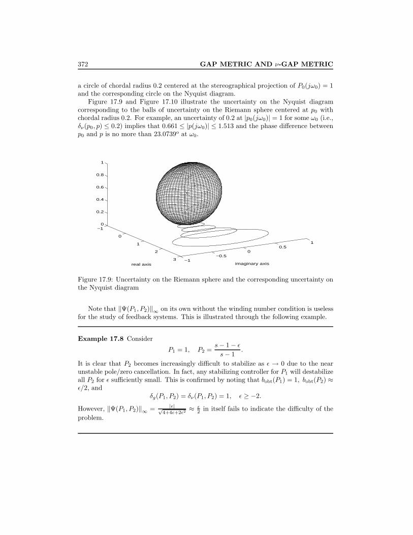
372 GAP METRIC AND ν-GAP METRIC
a circle of chordal radius 0.2 centered at the stereographical projection of P0(jω0) = 1and the corresponding circle on the Nyquist diagram.
Figure 17.9 and Figure 17.10 illustrate the uncertainty on the Nyquist diagramcorresponding to the balls of uncertainty on the Riemann sphere centered at p0 withchordal radius 0.2. For example, an uncertainty of 0.2 at |p0(jω0)| = 1 for some ω0 (i.e.,δν(p0, p) ≤ 0.2) implies that 0.661 ≤ |p(jω0)| ≤ 1.513 and the phase difference betweenp0 and p is no more than 23.0739o at ω0.
−1
0
1
2
3 −1−0.5
00.5
1
0
0.2
0.4
0.6
0.8
1
real axis imaginary axis
Figure 17.9: Uncertainty on the Riemann sphere and the corresponding uncertainty onthe Nyquist diagram
Note that ‖Ψ(P1, P2)‖∞ on its own without the winding number condition is uselessfor the study of feedback systems. This is illustrated through the following example.
Example 17.8 Consider
P1 = 1, P2 =s− 1− εs− 1
.
It is clear that P2 becomes increasingly difficult to stabilize as ε → 0 due to the nearunstable pole/zero cancellation. In fact, any stabilizing controller for P1 will destabilizeall P2 for ε sufficiently small. This is confirmed by noting that bobt(P1) = 1, bobt(P2) ≈ε/2, and
δg(P1, P2) = δν(P1, P2) = 1, ε ≥ −2.
However, ‖Ψ(P1, P2)‖∞ = |ε|√4+4ε+2ε2
≈ ε2 in itself fails to indicate the difficulty of the
problem.

17.4. Extended Loop-Shaping Design 373
0 0.5 1 1.5 2−1
−0.5
0
0.5
1
Real Axis
Imag
inar
y A
xis
p0=0.1
p0=0.5
p0=1
p0=1.5
23.0739 degree
Figure 17.10: Uncertainty on the Nyquist diagram corresponding to the balls of uncer-tainty on the Riemann sphere centered at p0 with chordal radius 0.2
17.4 Extended Loop-Shaping Design
Let P be a family of parametric uncertainty systems and let P0 ∈ P be a nominal designmodel. We are interested in finding a controller so that we have the largest possiblerobust stability margin; that is,
supK
infP∈P
bP,K .
Note that by Theorem 17.8, for any P1 ∈ P , we have
arcsin bP1,K(ω) ≥ arcsin bP0,K(ω)− arcsinψ(P0(jω), P1(jω)), ∀ω.
Now suppose we need infP∈P bP,K > α. Then it is sufficient to have
arcsin bP0,K(ω)− arcsinψ(P0(jω), P1(jω)) > arcsinα, ∀ω, P1 ∈ P ;
that is,
bP0,K(ω) > sin (arcsinψ(P0(jω), P1(jω)) + arcsinα) , ∀ω, P1 ∈ P .
Let W (s) ∈ H∞ be such that
|W (jω)| ≥ sin (arcsinψ(P0(jω), P1(jω)) + arcsinα) , ∀ω, P1 ∈ P .

374 GAP METRIC AND ν-GAP METRIC
Then it is sufficient to guarantee
|W (jω)|bP0,K(ω)
< 1.
Let P0 = M−10 N0 be a normalized left coprime factorization and note that
1bP0,K(ω)
:= σ
([I
K(jω)
](I + P0(jω)K(jω))−1 M−1
0 (jω)
).
Then it is sufficient to find a controller so that∥∥∥∥∥[I
K
](I + P0K)−1
M−10 W
∥∥∥∥∥∞
< 1.
The process can be iterated to find the largest possible α.Combining the preceding robust stabilization idea and theH∞ loop-shaping in Chap-
ter 16, one can devise an extended loop-shaping design procedure as follows. (A moreadvanced loop-shaping procedure can be found in Vinnicombe [1993b].)
Design Procedure:
Let P be a family of parametric uncertain systems and let P0 be a nominal model.
(a) Loop-Shaping: The singular values of the nominal plant are shaped, using a prec-ompensator W1 and/or a postcompensator W2, to give a desired open-loop shape.The nominal plant P0 and the shaping functions W1,W2 are combined to formthe shaped plant, Ps, where Ps = W2P0W1. We assume that W1 and W2 are suchthat Ps contains no hidden modes.
(b) Compute frequency-by-frequency:
f(ω) = supP∈P
ψ(Ps(jω),W2(jω)P (jω)W1(jω)).
Set α = 0.
(b) Fit a stable and minimum phase rational transfer function W (s) so that
|W (jω)| ≥ sin(arcsin f(ω) + arcsinα) ∀ω.
(c) Find a K∞ such that
β := infK∞
∥∥∥∥∥[
I
K∞
](I + P0K∞)−1
M−10 W
∥∥∥∥∥∞
.
(d) If β ≈ 1, stop and the final controller is K = W1K∞W2. If β 1, increase α andgo back to (b). If β 1, decrease α and go back to (b).

17.5. Controller Order Reduction 375
17.5 Controller Order Reduction
The controller order-reduction procedure described in Chapter 15 can, of course, beapplied to the loop-shaping controller design in Chapter 16 and the gap or ν-gap metricoptimization here. However, the controller order-reduction in the loop-shaping con-troller design, or gap metric, or ν-gap metric optimization is especially simple. Thefollowing theorem follows immediately from Theorems 17.7 and 17.10.
Theorem 17.11 Let P0 be a nominal plant and K0 be a stabilizing controller suchthat bP0,K0 ≤ bobt(P0). Let K0 = UV −1 be a normalized coprime factorization and letU , V ∈ RH∞ be such that ∥∥∥∥∥
[U
V
]−[U
V
]∥∥∥∥∥∞
≤ ε.
Then K := U V −1 stabilizes P0 if ε < bP0,K0. Furthermore,
arcsin bP,K ≥ arcsin bP0,K0 − arcsin ε− arcsinβ
for all P : δν(P, P0) ≤ β.
Hence to reduce the controller order one only needs to approximate the normalizedcoprime factors of the controller. An algorithm for finding the best approximation isalso presented in Vinnicombe [1993a, 1993b].
17.6 Notes and References
This chapter is based on Georgiou and Smith [1990] and Vinnicombe [1993a, 1993b].Early studies of the gap metric can be found in Zames and El-Sakkary [1980] and El-Sakkary [1985]. The pointwise gap metric was introduced by Qiu and Davision [1992b].
17.7 Problems
Problem 17.1 Calculate the gap δg(Pi, Pj) with
P1 =1
s+ 1, P2 =
1s− 1
, P3 =s+ 2
(s+ 1)2, P4 =
s− 2(s+ 1)2
, P5 =1
(s+ 1)2.
Problem 17.2 Let P = 10τs+1 , τ ∈ [1, 3] and let P0 = 10
τ0s+1 . Find the optimal τ0 ∈ [1, 3]minimizing
minτo
maxτ
δg(P, P0).
Problem 17.3 Repeat Problems 17.1–17.2 for the ν-gap metric.

376 GAP METRIC AND ν-GAP METRIC

Chapter 18
Miscellaneous Topics
This chapter considers two somewhat different problems. The first section gives a briefintroduction into the problem of model validation and the second section considers themixed real and complex µ analysis and synthesis.
18.1 Model Validation
A key to the success of the robust control theory developed in this book is to haveappropriate descriptions of the uncertain system (whether it is an additive uncertaintymodel or a general linear fractional model). Then an important question is how one candecide if a model description is appropriate (i.e., how to validate a model).
For simplicity of presentation, we have chosen to present the discrete time modelvalidation in this section with the understanding that a continuous time problem can beapproximated by fast sampling. Suppose we have modeled a set of uncertain dynamicalsystems by
∆ := ∆ : ∆ ∈ H∞, ‖∆‖∞ ≤ 1
where the H∞ norm of a discrete time system ∆ ∈ H∞ is defined as ‖∆(z)‖∞ =sup|z|>1 σ (∆(z)). In order to verify whether this model assumption is correct, someexperimental data are collected. For example, let the input to the system be the sequenceu = (u0, u1, . . . , ul−1) and the output y = (y0, y1, . . . , yl−1). A natural question iswhether these data are consistent with our modeling assumption. In other words, doesthere exist a model ∆ ∈ ∆ such that the output of the ∆ for the period of t =0, 1, . . . , l − 1 is exactly y = (y0, y1, . . . , yl−1) with the input u = (u0, u1, . . . , ul−1)? Ifthere does not exist a such ∆, then the model is invalidated. If there exists a such ∆,however, it does not mean that the model is validated but it only means that the modelis not validated by this set of data and it may be invalidated by another set of data inthe future. Hence it is actually more accurate to say our validation procedure is modelinvalidation.
377

378 MISCELLANEOUS TOPICS
Let ∆ be a stable, causal, linear, time-invariant system with transfer matrix
∆(z) = h0 + h1z−1 + h2z
−2 + · · ·
where hi, i = 0, 1, . . . are the matrix Markov parameters. Suppose we have applied theinput sequence u = (u0, u1, . . . , ul−1) to the system and collected the output for theperiod t = 0, 1, . . . , `− 1, y = (y0, y1, . . . , yl−1). Then the input and output sequencesare related by a Toeplitz matrix:
y0
y1
...yl−1
=
h0 0 · · · 0
h1 h0. . . 0
......
. . . 0hl−1 hl−2 · · · h0
u0
u1
...ul−1
.
This equation shows that, for u0 6= 0 and SISO ∆, the inputs and outputs uniquelydetermine the first ` Markov parameters of the transfer function ∆(z). The model isvalidated (or more accurately not invalidated) if the remaining Markov parameters canbe chosen so that ∆(z) ∈ ∆. The existence of such a choice is the classical tangentialCaratheodory-Fejer interpolation problem, for which a solution to the MIMO case canbe found in Foias and Frazho [1990, page 195]. We shall state this result in the followingtheorem. But we shall define some notation first.
Let (v0, v1, . . . , v`−1, v`, v`+1, . . .) be a sequence and let π` denote the truncationoperator such that
π`(v0, v1, . . . , v`−1, v`, v`+1, . . .) = (v0, v1, . . . , v`−1).
Let v = (v0, v1, . . . , v`−1) be a sequence of vectors and denote
Tv :=
v0 0 · · · 0
v1 v0. . . 0
......
. . . 0vl−1 vl−2 · · · v0
.
Theorem 18.1 Given u = (u0, u1, . . . , ul−1) and y = (y0, y1, . . . , yl−1), there exists a∆ ∈ H∞, ‖∆‖∞ ≤ 1 such that
y = π`∆u
if and only if T ∗y Ty ≤ T ∗uTu.
Note that the output of ∆ after time t = `− 1 is irrelevant to the test. The conditionT ∗y Ty ≤ T ∗uTu is equivalent to
i∑j=1
‖yj‖2 ≤i∑
j=1
‖uj‖2 , i = 0, 1, . . . , `− 1

18.1. Model Validation 379
or‖πiy‖2 ≤ ‖πiu‖2 , i = 0, 1, . . . , `− 1,
which is obviously necessary. In fact, the last condition holds for stable, linear, time-varying operator ∆ with supu6=0
‖∆u‖2‖u‖2
≤ 1; see Poolla et al. [1994]. Note that ifu0 6= 0, then Tu is of full column rank and the condition can also be written asσ(Ty(T ∗uTu)−
12
)≤ 1.
Using the above theorem, we can derive solutions to some model validation problemseasily. For example, consider a set of additive models shown in Figure 18.1.
f f P (z)
∆(z) W (z)
?
D(z)
?
?y
d
u
Figure 18.1: Model validation for additive uncertainty
In this case,y = (P + ∆W )u+Dd, ‖∆‖∞ ≤ 1
where P (z),W (z), D(z) and ∆(z) are causal, linear, time-invariant systems (but notnecessarily stable). The disturbance d is assumed to come from a convex set, d ∈ Dconvex;for example, Dconvex = d : d ∈ `2[0,∞), ‖d‖2 ≤ 1. For simplicity, we shall also assumethat W (∞) is of full column rank. Let
D(z) = D0 +D1z−1 +D2z
−2 + · · · .
Theorem 18.2 Given a set of input-output data uexpt = (u0, u1, . . . , u`−1) with u0 6= 0,yexpt = (y0, y1, . . . , y`−1) for the additive perturbed uncertainty system with an additivedisturbance d ∈ Dconvex, where Dconvex is a convex set, let
u = (u0, u1, . . . , u`−1) = π`(Wuexpt)
y = (y0, y1, . . . , y`−1) = yexpt − π`Puexpt.
Then there exists a ∆ ∈ H∞, ‖∆‖∞ ≤ 1 such that
yexpt = π` ((P + ∆W )uexpt +Dd)
for some d ∈ Dconvex if and only if there exists a d = (d0, d1, . . . , dl−1) ∈ π`Dconvex suchthat
σ[(Ty − TDTd)(T ∗uTu)−1/2
]≤ 1

380 MISCELLANEOUS TOPICS
where
TD :=
D0 0 · · · 0
D1 D0. . . 0
......
. . . 0Dl−1 Dl−2 · · · D0
.
Proof. Note that the system input-output equation can be written as
(y − Pu)−Dd = ∆(Wu).
Since P,W,D, and ∆ are causal, linear, and time invariant, we have π`Dd = π`Dπ`d,π`(y − Pu) = yexpt − π`Pπ`u = yexpt − π`Puexpt and π`Wu = π`Wπ`u = π`Wuexpt.Denote
d = (d0, d1, . . . , d`−1) = π`(Dd).
Then it is easy to show that d0
d1
...d`−1
= TD
d0
d1
...d`−1
and Td = TDTd. Now note that
Tπ`(y−Pu−Dd) = Tπ`(y−Pu) − Tπ`(Dd) = Ty − TDTd, Tπ`Wu = Tu
and π`∆Wu = π`∆π`(Wu) since ∆ is causal. Applying Theorem 18.1, there exists a∆ ∈ H∞, ‖∆‖∞ ≤ 1 such that
π` [(y − Pu)−Dd] = π`∆(Wu) = π`∆π`(Wu)
if and only if(Ty − TDTd)∗(Ty − TDTd) ≤ T ∗uTu
which is equivalent toσ[(Ty − TDTd)(T ∗uTu)−
12
]≤ 1.
Note that Tu is of full column rank since W (∞) is of full column rank and u0 6= 0,which implies u0 6= 0. 2
Note thatinf
d∈Dconvexσ[(Ty − TDTd)(T ∗uTu)−
12
]≤ 1
is a convex problem and can be checked numerically.

18.2. Mixed µ Analysis and Synthesis 381
Many other classes of model validation problems can be solved analogously. Forexample, consider a coprime factor model validation problem with
y = (M + ∆MWM )−1(N + ∆NWN )u+ d
where M,N,WM , and WN are causal, linear, time-invariant systems, and ∆M ,∆N ∈H∞,
[∆M ∆N
]∞≤ 1. Then the problem can be solved by multiplying M+∆MWM
from the left of the system equation and rewriting the system equation as
(My −Nu−Md) =[
∆M ∆N
] [ WM (d− y)WNu
].
The model validation of a general LFT uncertainty system is considered in Davis [1995]and Chen and Wang [1996]. For continuous time model validation, see Rangan andPoolla [1996] and Smith and Dullerud [1996].
18.2 Mixed µ Analysis and Synthesis
In Chapter 10, we considered analysis and synthesis of systems with complex uncertain-ties. However, in practice, many systems involve parametric uncertainties that are real(for example, the uncertainty about a spring constant in a mechanical system). In thiscase, one has to cover this real parameter variation with a complex disk in order touse the complex µ analysis and synthesis tools, which usually results in a conservativesolution. In this section, we shall consider briefly the analysis and synthesis problemswith possibly both real parametric and complex uncertainties.
The mixed real and complex µ involves three types of blocks: repeated real scalar,repeated complex scalar, and full blocks. Three nonnegative integers, Sr, Sc, and F ,represent the number of repeated real scalar blocks, the number of repeated complexscalar blocks, and the number of full blocks, and they satisfy
Sr∑i=1
ki +Sc∑i=1
ri +F∑j=1
mj = n.
The ith repeated real scalar block is ki × ki, the jth repeated complex scalar block isrj×rj , and the `th full block is m`×m`. The admissible set of uncertainties ∆ ⊂ Cn×nis defined as
∆ =
diag[φ1Ik1 , . . . , φsrIksr , δ1Ir1 , . . . , δscIrsc ,
∆1, . . . ,∆F ] : φi ∈ R, δj ∈ C, ∆` ∈ Cm`×m`. (18.1)
The mixed µ is defined in the same way as for the complex µ: Let M ∈ Cn×n; then
µ∆(M) := (min σ(∆) : ∆ ∈∆,det (I −M∆) = 0)−1 (18.2)

382 MISCELLANEOUS TOPICS
unless no ∆ ∈∆ makes I−M∆ singular, in which case µ∆(M) := 0. Or, equivalently,
1µ∆(M)
:= inf α : det(I − αM∆) = 0, σ(∆) ≤ 1, ∆ ∈∆ .
Let ρR(M) be the real spectral radius (i.e., the largest magnitude of the real eigen-values of M). For example, if a 4 × 4 matrix M has eigenvalues 1 ± j3,−2, 1, thenρ(M) = |1 + j3| =
√10 and ρR(M) = | − 2| = 2. It is easy to see that
µ∆(M) = max∆∈B∆
ρR(M∆)
where B∆ := ∆ : ∆ ∈∆, σ(∆) ≤ 1. Note that max∆∈B∆
ρR(M∆) = max∆∈B∆
ρ(M∆) if
sr = 0. [This should not be confused with the fact that, for a given matrix ∆ ∈ B∆and M , ρR(M∆) may not be equal to ρ(M∆). For example, M = 2ej
π4 and ∆ = 1;
then ρ(M∆) = 2 but ρR(M∆) = 0 since M has no real eigenvalues. However, one canchoose another ∆1 = e−j
π4 such that ρR(M∆1) = 2 = ρ(M∆).]
DefineQ = ∆ ∈∆ : φi ∈ [−1, 1], |δi| = 1, ∆i∆∗i = Imi
D =
diag
[D1, . . . , Dsr , D1, . . . , Dsc , d1Im1 , . . . , dF−1ImF−1 , ImF
]:
Di ∈ Cki×ki , Di = D∗i > 0, Di ∈ Cri×ri , Di = D∗i > 0, dj ∈ R, dj > 0
.
G =
diag [G1, . . . , Gsr , 0, . . . , 0] : Gi = G∗i ∈ Cki×ki.
It was shown in Young [1993] that
µ∆(M) = maxQ∈Q
ρR(QM).
Note that the above maximization is not necessarily achieved on the vertices for thereal parameters; hence one must search over the entire interval for each real parameter.Again this maximization problem can have many local maximums and a power algorithmhas been developed in Young [1993] to compute a lower bound.
It should also be noted that even though the complex µ (i.e., sr = 0) is a continuousfunction of the data, the mixed µ (i.e., sr 6= 0) may only be upper semicontinuous; seePackard and Pandey [1993]. It was also shown in Braatz et al. [1994] and Toker andOzbay [1995] that the computation of µ is a NP hard problem, which means that itmay not be computable in a polynomial time. Of course, it should not be interpretedas every µ problem will not be solvable in a polynomial time; merely some might not.
Obviously, the upper bound for the complex µ can be applied for the mixed µ whenthe intervals of the real parameters are covered by complex disks. However, a betterbound can be obtained for the mixed µ by exploiting the phase information of the realparameters. To motivate the improved bound for the mixed µ, we consider again theupper bound for the complex µ problem. It is known that
µ∆(M) ≤ infD∈D
σ(DMD−1).

18.2. Mixed µ Analysis and Synthesis 383
This bound can be reformulated using linear matrix inequalities by noting the following:
σ(DMD−1) ≤ β ⇐⇒ (DMD−1)∗DMD−1 ≤ β2I ⇐⇒ M∗D∗DM − β2D∗D ≤ 0.
Since D is nonsingular and D∗D ∈ D, we have
µ∆(M) ≤ infD∈D
minβ
β : M∗DM − β2D ≤ 0
.
The following upper bound for the mixed µ was derived by Fan, Tits, and Doyle [1991]and reformulated in the current form by Young [1993].
Theorem 18.3 Let M ∈ Cn×n and ∆ ∈∆. Then
µ∆(M) ≤ infD∈D,G∈G
minβ
β : M∗DM + j(GM −M∗G)− β2D ≤ 0
.
Proof. Suppose we have a Q ∈ Q such that QM has a real eigenvalue λ ∈ R. Thenthere is a vector x ∈ Cn such that
QMx = λx.
Let D ∈ D. Then D12 ∈ D, D
12Q = QD
12 and
D12QMx = QD
12Mx = λD
12x.
Since σ(Q) ≤ 1, it follows that
λ2∥∥∥D 1
2x∥∥∥2
=∥∥∥QD 1
2Mx∥∥∥2
≤∥∥∥D 1
2Mx∥∥∥2
.
Hencex∗(M∗DM − λ2D)x ≥ 0.
Next, let G ∈ G and note that Q∗G = QG = GQ; then
x∗GMx =(
1λQMx
)∗GMx =
1λx∗M∗Q∗GMx =
1λx∗M∗QGMx
=1λx∗M∗GQMx =
1λx∗M∗G(QMx) = x∗M∗Gx.
That is,x∗(GM −M∗G)x = 0.
Note that j(GM −M∗G) is a Hermitian matrix, so it follows that for such x
x∗(M∗DM + j(GM −M∗G)− λ2D)x ≥ 0.
It is now easy to see that if we have D ∈ D, G ∈ G and 0 ≤ β ∈ R such that
M∗DM + j(GM −M∗G)− β2D ≤ 0

384 MISCELLANEOUS TOPICS
then |λ| ≤ β, and hence µ∆(M) ≤ β. 2
This upper bound has an interesting interpretation: covering the uncertainties onthe real axis using possibly off-axis disks. To illustrate, let M ∈ C be a scalar and∆ ∈ [−1, 1]. We can cover this real interval using a disk as shown in Figure 18.2.
The off-axis disk can be expressed as
jG
β+
√1 +
(G
β
)2
∆, ∆ ∈ C,∣∣∣∆∣∣∣ ≤ 1.
Centered Disk Off-Axis Disk
Re Re
Im
11
βj G
-1-1
-j
Im
j
Figure 18.2: Covering real parameters with disks
Hence 1−∆Mβ 6= 0 for all ∆ ∈ [−1, 1] is guaranteed if
1−
jGβ
+
√1 +
(G
β
)2
∆
M
β6= 0, ∆ ∈ C,
∣∣∣∆∣∣∣ ≤ 1
⇐⇒ 1−
√1 +
(Gβ
)2Mβ
1− jGβMβ
∆ 6= 0, ∆ ∈ C,∣∣∣∆∣∣∣ ≤ 1
⇐⇒
√
1 +(Gβ
)2Mβ
1− jGβMβ
∗
√1 +
(Gβ
)2Mβ
1− jGβMβ
≤ 1
⇐⇒ M∗
β
M
β+ j(
G
β
M
β− M∗
β
G
β)− 1 ≤ 0
⇐⇒ M∗M + j(GM −M∗G)− β2 ≤ 0.

18.2. Mixed µ Analysis and Synthesis 385
The scaling G allows one to exploit the phase information about the real parameters sothat a better upper bound can be obtained. We shall demonstrate this further using asimple example.
Example 18.1 Let
G(s) =s2 + 2s+ 1
s3 + s2 + 2s+ 1.
Nyquist diagram 1/G
disk centered at (0,0)
disk centered at (0,−0.2j)
disk centered at (0, −j)
−1.5 −1 −0.5 0 0.5 1 1.5−2
−1.5
−1
−0.5
0
0.5
1
Figure 18.3: Computing the real stability margin by covering with disks
We are interested in finding the largest k such that 1 + ∆G(s) has no zero in theright-half plane for all ∆ ∈ [−k, k]. Of course, the largest k can be found very easily byusing well-known stability test, which gives
kmax =(
supωµ∆(G(jω))
)−1
=(
supω
maxφ∈[−1,1]
ρR(φG(jω)))−1
=(
supω|G(jω)| : =G(jω) = 0
)−1
= infω
1
|G(jω)| : =G(jω) = 0
= 0.5.

386 MISCELLANEOUS TOPICS
Now we use the complex covering idea to find the best possible k. Note that we onlyneed to find the smallest |∆| so that 1 + ∆G(jω0) = 0 for some ω0 or, equivalently,∆ + 1/G(jω0) = 0. The frequency response of 1/G and the disks covering an interval[−k, k] are shown in Figure 18.3. It is clear that a centered disk would give k =1/ ‖G‖∞ = 0.2970 and an off-axis disk centered at (0,−0.2j) would give k = 0.3984while an off-axis disk centered at (0,−j) would give the exactly value k = 0.5.
The following alternative characterization of the upper bound is useful in the mixedµ synthesis.
Theorem 18.4 Given β > 0, there exist D ∈ D and G ∈ G such that
M∗DM + j(GM −M∗G)− β2D ≤ 0
if and only if there are D1 ∈ D and G1 ∈ G such that
σ
((D1MD−1
1
β− jG1
)(I +G2
1)−12
)≤ 1.
Proof. Let D = D21 and G = βD1G1D1. Then
M∗DM + j(GM −M∗G)− β2D ≤ 0
⇐⇒ M∗D21M + j(βD1G1D1M − βM∗D1G1D1)− β2D2
1 ≤ 0
⇐⇒ (D1MD−11 )∗(D1MD−1
1 ) + j(βG1D1MD−11 − β(D1MD−1
1 )∗G1)− β2I ≤ 0
⇐⇒(D1MD−1
1
β− jG1
)∗(D1MD−1
1
β− jG1
)− (I +G2
1) ≤ 0
⇐⇒ σ
[(D1MD−1
1
β− jG1
)(I +G2
1)−12
]≤ 1.
2
Similarly, the following corollary can be shown.
Corollary 18.5 µ∆(M) ≤ rβ if there are D1 ∈ D and G1 ∈ G such that
σ
((D1MD−1
1
β− jG1
)(I +G2
1)−12
)≤ r ≤ 1.

18.2. Mixed µ Analysis and Synthesis 387
Proof. This follows by noting that
σ
((D1MD−1
1
β− jG1
)(I +G2
1)−12
)≤ r ≤ 1
=⇒(D1MD−1
1
rβ− jG1
r
)∗(D1MD−1
1
rβ− jG1
r
)≤ I +G2
1 ≤ I +(G1
r
)2
.
Let G2 =G1
r∈ G. Then
(D1MD−1
1
rβ− jG2
)∗(D1MD−1
1
rβ− jG2
)≤ I +G2
2
=⇒ σ
((D1MD−1
1
rβ− jG2
)(I +G2
2)−12
)≤ 1
=⇒ µ∆(M) ≤ rβ.
2
Note that this corollary is not necessarily true if r > 1. It is fairly easy to checkthat the well-posedness condition, main loop theorem, robust stability, and robust per-formance theorems for the mixed µ setup are exactly the same as the ones for complexµ problems.
We are now in the position to consider the synthesis problem with mixed uncer-tainties. Consider again the general system diagram in Figure 18.4. By the robustperformance condition, we need to find a stabilizing controller K so that
minK
supωµ∆ (F`(P,K)) ≤ β.
wz
-
P
K
Figure 18.4: Synthesis framework
By Theorems 18.3 and 18.4, µ∆ (F` (P (jω),K(jω))) ≤ β, ∀ω if there are frequency-dependent scaling matrices Dω ∈ D and Gω ∈ G such that
supωσ
[(Dω (F` (P (jω),K(jω)))D−1
ω
β− jGω
)(I +G2
ω)−12
]≤ 1, ∀ω.

388 MISCELLANEOUS TOPICS
Similar to the complex µ synthesis, we can now describe a mixed µ synthesis procedurethat involves D,G−K iterations.
D,G−K Iteration:
(1) Let K be a stabilizing controller. Find initial estimates of the scaling matricesDω ∈ D, Gω ∈ G and a scalar β1 > 0 such that
supωσ
[(Dω (F` (P (jω),K(jω)))D−1
ω
β1− jGω
)(I +G2
ω)−12
]≤ 1, ∀ω.
Obviously, one may start with Dω = I, Gω = 0, and a large β1 > 0.
(2) Fit the frequency response matrices Dω and jGω with D(s) and G(s) so that
D(jω) ≈ Dω, G(jω) ≈ jGω , ∀ ω.
Then for s = jω
supωσ
((Dω (F` (P (jω),K(jω)))D−1
ω
β1− jGω
)(I +G2
ω)−12
)
≈ supωσ
[(D(s) (F` (P (s),K(s)))D−1(s)
β1−G(s)
)(I +G∼(s)G(s))−
12
].
(3) Let D(s) be factorized as
D(s) = Dap(s)Dmin(s), D∼ap(s)Dap(s) = I, Dmin(s), D−1min(s) ∈ H∞.
That is, Dap is an all-pass and Dmin is a stable and minimum phase transfermatrix. Find a normalized right coprime factorization
D∼ap(s)G(s)Dap(s) = GNG−1M , GN , GM ∈ H∞
such thatG∼MGM +G∼NGN = I.
ThenG−1M D∼ap(I +G∼G)−1Dap(G−1
M )∼ = I
and, for each frequency s = jω, we have
σ
[(D(s) (F` (P (s),K(s)))D−1(s)
β1−G(s)
)(I +G∼(s)G(s))−
12
]
= σ
[(Dmin (F` (P,K))D−1
min
β1−D∼apGDap
)D∼ap(I +G∼G)−
12
]

18.3. Notes and References 389
= σ
[(Dmin (F` (P,K))D−1
min
β1−GNG−1
M
)D∼ap(I +G∼G)−
12
]
= σ
[(Dmin (F` (P,K))D−1
minGMβ1
−GN)G−1M D∼ap(I +G∼G)−
12
]
= σ
[Dmin (F` (P,K))D−1
minGMβ1
−GN].
(4) Define
Pa =
[Dmin(s)
I
]P (s)
[D−1
min(s)GM (s)I
]− β1
[GN
0
]
and find a controller Knew minimizing ‖F`(Pa,K)‖∞.
(5) Compute a new β1 as
β1 = supω
infDω∈D,Gω∈G
β(ω) : Γ ≤ 1
where
Γ := σ
[(DωF`(P,Knew)D−1
ω
β(ω)− jGω
)(I + G2
ω)−12
].
(6) Find Dω and Gω such that
infDω∈D,Gω∈G
σ
[(DωF`(P,Knew)D−1
ω
β1− jGω
)(I + G2
ω)−12
].
(7) Compare the new scaling matrices Dω and Gω with the previous estimates Dω
and Gω. Stop if they are close, else replace Dω, Gω and K with Dω, Gω andKnew, respectively, and go back to step (2).
18.3 Notes and References
The model validation problems are discussed in Smith and Doyle [1992] in the frequencydomain; in Poolla, Khargonekar, Tikku, Krause, Nagpal [1994 in the discrete timedomain (on which Section 18.1 is based); and in Rangan and Poolla [1996] and Smithand Dullerud [1996] in the continuous time domain. See also Davis [1995] and Chenand Wang [1996]. The mixed µ problems are discussed in detail in Young [1993] (onwhich Section 18.2 is based), Fan, Tits, and Doyle [1991], Packard and Pandey [1993],and references therein.

390 MISCELLANEOUS TOPICS
18.4 Problems
Problem 18.1 Write a Matlab program for the additive model validation problemand try it on a simple experiment in your laboratory.

Bibliography
[1] Al-Saggaf, U. M. and G. F. Franklin (1987). “An error bound for a discrete reducedorder model of a linear multivariable system,” IEEE Trans. Automat. Contr., Vol.AC-32, pp. 815-819.
[2] Al-Saggaf, U. M. and G. F. Franklin (1988). “Model reduction via balanced realiza-tions: an extension and frequency weighting techniques,” IEEE Trans. Automat.Contr., Vol. AC-33, No. 7, pp. 687-692.
[3] Anderson, B. D. O. (1967). “An algebraic solution to the spectral factorizationproblem,” IEEE Trans. Automat. Contr., Vol. AC-12, pp. 410-414.
[4] Anderson, B. D. O. (1993). “Bode Prize Lecture (Control design: moving fromtheory to practice),” IEEE Control Systems, Vol. 13, No.4, pp. 16-25.
[5] Anderson, B. D. O. and Y. Liu (1989). “Controller reduction: concepts and ap-proaches, ” IEEE Trans. Automat. Contr. , Vol. AC-34, No. 8, pp. 802-812.
[6] Anderson, B. D. O. and J. B. Moore (1989). Optimal Control: Linear QuadraticMethods. Prentice Hall, Englewood Cliffs, New Jersey.
[7] Anderson, B. D. O. and S. Vongpanitlerd (1973). Network Analysis and Synthesis:A Modern System Theory Approach. Prentice Hall, Englewood Cliffs, New Jersey.
[8] Arnold, W. F. and A. J. Laub (1984). “Generalized Eigenproblem algorithms andsoftware for algebraic Riccati equations,” Proceedings of the IEEE, Vol. 72, No.12, pp. 1746-1754.
[9] Balas, G. (1990). Robust Control of Flexible Structures: Theory and Experiments,PhD. Thesis, California Institute of Technology.
[10] Balas, G., J. C. Doyle, K. Glover, A. Packard, and R. Smith (1994). µ-Analysisand Synthesis Toolbox, MUSYN Inc. and The MathWorks, Inc.
[11] Basar, T. and P. Bernhard (1991). H∞-Optimal Control and Related MinimaxDesign Problems: A Dynamic Game Approach. Systems and Control: Foundationsand Applications. Birkhauser, Boston.
391

392 BIBLIOGRAPHY
[12] Bernstein, D. S. and W. M. Haddard (1989). “LQG control with an H∞ perfor-mance bound: A Riccati equation approach,” IEEE Trans. Automat. Contr., Vol.AC-34, pp. 293-305.
[13] Bode, H. W. (1945). Network Analysis and Feedback Amplifier Design, Van Nos-trand, Princeton.
[14] Boyd, S., V. Balakrishnan, and P. Kabamba (1989). “A bisection method for com-puting the H∞ norm of a transfer matrix and related problems,” Math. Control,Signals, and Systems, Vol. 2, No. 3, pp. 207-220.
[15] Boyd, S. and C. Barratt (1991). Linear Controller Design -Limits of Performance,Prentice Hall, Englewood Cliffs, New Jersey.
[16] Boyd, S. and C. A. Desoer (1985). “Subharmonic functions and performancebounds in linear time-invariant feedback systems,” IMA J. Math. Contr. andInfo., Vol. 2, pp. 153-170.
[17] Boyd, S., L. El Ghaoui, E. Feron, and V. Balakrishnan (1994). Linear MatrixInequalities in Systems and Control Theory, SIAM, Philadelphia.
[18] Braatz, R. D., P. M. Young, J. C. Doyle, and M. Morari (1994). “Computationalcomplexity of µ calculation,” IEEE Trans. Automat. Contr., Vol. 39, No. 5, pp.1000-1002.
[19] Brogan, W. L. (1991). Modern Control Theory, 3rd ed., Prentice Hall, EnglewoodCliffs, New Jersey.
[20] Bruinsma, N. A. and M. Steinbuch (1990). “A fast algorithm to compute theH∞-norm of a transfer function matrix”, Systems and Control Letters, Vol. 14,pp. 287-293.
[21] Bryson Jr., A. E. and Y-C. Ho (1975). Applied Optimal Control, HemispherePublishing Corporation.
[22] Chen, C. T. (1984). Linear System Theory and Design, Holt, Rinehart and Win-ston.
[23] Chen, J. (1995). “Sensitivity integral relations and design trade-offs in linear mul-tivariable feedback systems,” IEEE Trans. Auto. Contr., Vol. 40, No. 10, pp.1700-1716.
[24] Chen, J. and S. Wang (1996). “Validation of linear fractional uncertain models:solutions via matrix inequalities,” IEEE Trans. Auto. Contr., Vol. 41, No. 6, pp.844-849.
[25] Chen, T. and B. A. Francis (1992). “H2-optimal sampled-data control,” IEEETrans. Automat. Contr., Vol. 36, No. 4, pp. 387-397.

BIBLIOGRAPHY 393
[26] Chen, X. and K. Zhou (1996). “On the algebraic approach to H∞ control,” 1996IFAC World Congress, San Francisco, California, pp. 505-510.
[27] Chilali, M. and P. Gahinet (1996). “H∞ design with pole placement constraints:an LMI approach,” IEEE Trans. Automat. Contr., Vol. 41, No. 3, pp. 358-367.
[28] Christian, L. and J. Freudenberg (1994). “Limits on achievable robustness againstcoprime factor uncertainty,” Automatica, Vol. 30, No. 11, pp. 1693-1702.
[29] Chu, C. C. (1985).H∞ optimization and robust multivariable control. Ph.D. thesis,University of Minnesota.
[30] Dahleh, M. and I. J. Diaz-Bobillo (1995). Control of Uncertain Systems: A LinearProgramming Approach, Prentice Hall, Englewood Cliffs, New Jersey.
[31] Daniel, R. W., B. Kouvaritakis, and H. Latchman (1986). “Principal directionalignment: a geometric framework for the complete solution to the µ problem,”IEE Proceedings, Vol. 133, Part D, No. 2, pp. 45-56.
[32] Davis, R. A. (1995). Model Validation for Robust Control, Ph.D. dissertation,University of Cambridge, UK.
[33] Desoer, C. A., R. W. Liu, J. Murray, and R. Saeks (1980). “Feedback systemdesign: the fractional representation approach to analysis and synthesis,” IEEETrans. Automat. Contr., Vol. AC-25, No. 6, pp. 399-412.
[34] Desoer, C. A. and M. Vidyasagar (1975). Feedback Systems: Input-Output Prop-erties, Academic Press, New York.
[35] Doyle, J. C. (1978). “Guaranteed Margins for LQG Regulators,” IEEE Trans.Automat. Contr., Vol. AC-23, No. 4, pp. 756-757.
[36] Doyle, J.C. (1982). “Analysis of feedback systems with structured uncertainties,”IEE Proceedings, Part D, Vol.133, pp. 45-56.
[37] Doyle, J. C. (1984). “Lecture notes in advances in multivariable control,”ONR/Honeywell Workshop, Minneapolis.
[38] Doyle, J. C. (1985). “Structured uncertainty in control system design”, Proc.IEEE Conf. Dec. Contr., Ft. Lauderdale.
[39] Doyle, J. C., B. Francis, and A. Tannenbaum (1992). Feedback Control Theory,Macmillan Publishing Company.
[40] Doyle, J. C., K. Glover, P.P . Khargonekar, B. A. Francis (1989). “State-space so-lutions to standardH2 andH∞ control problems,” IEEE Trans. Automat. Contr.,Vol. AC-34, No. 8, pp. 831-847. Also see 1988 American Control Conference, At-lanta, June 1988.
394 BIBLIOGRAPHY
[41] Doyle, J., K. Lenz, and A. Packard (1986). “Design examples using µ synthesis:space shuttle lateral axis FCS during reentry,” IEEE Conf. Dec. Contr., December1986, pp. 2218-2223.
[42] Doyle, J. C., A. Packard and K. Zhou (1991). “Review of LFTs, LMIs and µ,”Proc. IEEE Conf. Dec. Contr., England, pp. 1227-1232
[43] Doyle, J. C., R. S. Smith, and D. F. Enns (1987). “Control of plants with inputsaturation nonlinearities,” American Control Conference, pp. 1034-1039.
[44] Doyle, J. C. and G. Stein (1981). “Multivariable feedback design: Concepts fora classical/modern synthesis,” IEEE Trans. Automat. Contr., Vol. AC-26, pp.4-16, Feb. 1981.
[45] Doyle, J. C., J. Wall and G. Stein (1982). “Performance and robustness analysisfor structured uncertainty,” in Proc. IEEE Conf. Dec. Contr., pp. 629-636.
[46] Doyle, J. C., K. Zhou, K. Glover, and B. Bodenheimer (1994). “Mixed H2 andH∞ performance objectives II: optimal control,” IEEE Trans. Automat. Contr.,Vol. 39, No. 8, pp. 1575-1587.
[47] El-Sakkary, A. (1985). “The gap metric: robustness of stabilization of feedbacksystems,” IEEE Trans. Automat. Contr., Vol. 30, pp. 240-247.
[48] Enns, D. (1984a). Model Reduction for Control System Design, Ph.D. dissertation,Department of Aeronautics and Astronautics, Stanford University, Stanford, Cal-ifornia.
[49] Enns, D. (1984b). “Model reduction with balanced realizations: an error boundand a frequency weighted generalization,” Proc. Conf. Dec. Contr., Las Vegas,Nevada.
[50] Fan, M. K. H. and A. L. Tits (1986). “Characterization and efficient computationof the structured singular value,” IEEE Trans. Automat. Contr., Vol. AC-31, No.8, pp. 734-743.
[51] Fan, M. K. H., A. L. Tits, and J. C. Doyle (1991). “Robustness in the presence ofmixed parametric uncertainty and unmodeled dynamics,” IEEE Trans. Automat.Contr., Vol. AC-36, No. 1, pp. 25-38.
[52] Foias, C. and A. E. Frazho (1990). The commutant Lifting Approach to Interpo-lation Problems, Birkhauser.
[53] Francis, B. A. (1987). A course in H∞ control theory, Lecture Notes in Controland Information Sciences, Vol. 88, Springer-Verlag.
[54] Francis, B. A. and J. C. Doyle (1987). “Linear control theory with an H∞ opti-mality criterion,” SIAM J. Contr. Optimiz., Vol. 25, pp. 815-844.

BIBLIOGRAPHY 395
[55] Franklin, G. F., J. D. Powell, and M. L. Workman (1990), Digital Control ofDynamic Systems, 2nd Ed, Addison-Wesley Publishing company.
[56] Freudenberg, J. S. (1986). “The general structured singular problem with twoblocks of uncertainty.” Proc. 1986 Allerton Conf., Monticello, Illinois.
[57] Freudenberg, J. S. and D. P. Looze (1988). Frequency Domain Properties of Scalarand Multivariable Feedback Systems, Lecture Notes in Contr. and Info. Science,Vol. 104, Springer-Verlag, Berlin.
[58] Gahinet, P. (1996). “Explicit controller formulas for LMI-based H∞ synthesis,”Automatica, Vol. 32, No. 7, pp. 1007-1014.
[59] Gahinet, P. and P. Apkarian (1994). “A linear matrix inequality approach to H∞control,” Int. J. Robust and Nonlinear Control, Vol. 4, pp. 421-448.
[60] Garnett, J. B. (1981). Bounded Analytic Functions, Academic Press.
[61] Georgiou, T. T. (1988). “On the computation of the gap metric,” Systems andControl Letters, Vol. 11, pp. 253-257.
[62] Georgiou, T. T. and M. C. Smith (1990). “Optimal robustness in the gap metric,”IEEE Trans. Automat. Contr., Vol. AC-35, No. 6, pp. 673-686.
[63] Georgiou, T. T. and M. C. Smith (1992). “Robust stabilization in the gap metric:controller design for distributed plants,” IEEE Trans. Automat. Contr., Vol. AC-37, No. 8, pp. 1133-1143.
[64] Glover, K. (1984). “All optimal Hankel-norm approximations of linear multivari-able systems and their L∞-error bounds,” Int. J. Contr., Vol. 39, pp. 1115-1193,1984.
[65] Glover, K. (1986a). “Robust stabilization of linear multivariable systems: Rela-tions to approximation,” Int. J. Contr., Vol. 43, No. 3, pp. 741-766.
[66] Glover, K. (1986b). “Multiplicative approximation of linear multivariable systemswith L∞ error bounds, ” Proc. Amer. Contr. Conf., Seattle, WA, pp. 1705-1709.
[67] Glover, K. and J. Doyle (1988). “State-space formulae for all stabilizing controllersthat satisfy an H∞ norm bound and relations to risk sensitivity,” Systems andControl Letters, Vol. 11, pp. 167-172.
[68] Glover, K. and J. C. Doyle (1989). “A state space approach to H∞ optimal con-trol,” in Three Decades of Mathematical Systems Theory: A Collection of Surveysat the Occasion of the 50th Birthday of Jan C. Willems, H. Nijmeijer and J. M.Schumacher (Eds.), Springer-Verlag, Lecture Notes in Control and InformationSciences, Vol. 135, 1989.
396 BIBLIOGRAPHY
[69] Glover, K., D. J. N. Limebeer, J. C. Doyle, E. M. Kasenally, and M. G. Safonov(1991). “A characterization of all solutions to the four block general distanceproblem,” SIAM J. Contr. Optimiz., Vol. 29, No. 2, pp. 283-324.
[70] Glover, K., D. J. N. Limebeer, and Y. S. Hung (1992). “A structured approxima-tion problem with applications to frequency weighted model reduction, ” IEEETrans. Automat. Contr., Vol. AC-37, No. 4, pp. 447-465.
[71] Glover, K. and D. McFarlane (1989). “Robust stabilization of normalized coprimefactor plant descriptions with H∞ bounded uncertainty,” IEEE Trans. Automat.Contr., Vol. 34, No. 8, pp. 821-830.
[72] Glover, K. and D. Mustafa (1989). “Derivation of the maximum entropy H∞controller and a state space formula for its entropy,” Int. J. Contr., Vol. 50, pp.899.
[73] Goddard, P. J. and K. Glover (1993). “Controller reduction: weights for stabilityand performance preservation,” Proceedings of the 32nd Conference on Decisionand Control, San Antonio, Texas, December 1993, pp. 2903-2908.
[74] Goddard, P. J. and K. Glover (1994). “Performance preserving frequency weightedcontroller approximation: a coprime factorization approach,” Proceedings of the33nd Conference on Decision and Control, Orlando, Florida, December 1994.
[75] Gohberg, I., and S. Goldberg (1981). Basic Operator Theory. Birkhauser, Boston.
[76] Gohberg, I., P. Lancaster, and L. Rodman (1986). “On Hermitian solutions of thesymmetric algebraic Riccati equation,” SIAM J. Contr. Optimiz., Vol. 24, No. 6,November 1986, pp. 1323-1334.
[77] Golub, G. H., and C. F. Van Loan (1983). Matrix Computations, Johns HopkindUniv. Press, Baltimore.
[78] Green, M. (1988). “A relative error bound for balanced stochastic truncation,”IEEE Trans. Automat. Contr., Vol. AC-33, No. 10, pp. 961-965.
[79] Green, M. (1992). “H∞ controller synthesis by J-lossless coprime factorization,”SIAM J. Contr. Optimiz., Vol. 30, No. 3, pp. 522-547.
[80] Green, M., K. Glover, D. J. N. Limebeer, and J. C. Doyle (1988), “A J-spectralfactorization approach to H∞ control,” SIAM J. Contr. Optimiz., Vol. 28, pp.1350-1371.
[81] Green, M. and D. J. N. Limebeer (1995). Linear Robust Control, Prentice Hall,Englewood Cliffs, New Jersey.
[82] Hinrichsen, D., and A. J. Pritchard (1990). “An improved error estimate forreduced-order models of discrete time system,” IEEE Trans. Automat. Contr.,AC-35, pp. 317-320.

BIBLIOGRAPHY 397
[83] Hoffman, K. (1962). Banach Spaces of Analytic Functions, Prentice Hall, Engle-wood Cliffs, New Jersey.
[84] Horn, R. A. and C. R. Johnson (1990). Matrix Analysis, Cambridge UniversityPress, first published in 1985.
[85] Horn, R. A. and C. R. Johnson (1991). Topics in Matrix Analysis, CambridgeUniversity Press.
[86] Horowitz, I. M. (1963). Synthesis of Feedback Systems, Academic Press, London.
[87] Hung, Y. S. (1989).“H∞-optimal control–Part I: model matching, – Part II: solu-tion for controllers,” Int. J. Contr., Vol. 49, pp. 1291-1359.
[88] Hung, Y. S. and K. Glover (1986). “Optimal Hankel-norm approximation of stablesystems with first order stable weighting functions,” Systems and Control Letters,Vol. 7, pp. 165-172.
[89] Hyde, R. A. and K. Glover (1993). “The application of scheduled H∞ controllersto a VSTOL aircraft,” IEEE Trans. Automat. Contr., Vol. 38, No. 7, pp. 1021-1039.
[90] Jonckheere, E. and L. M. Silverman (1983). “A new set of invariants for linearsystems - applications to reduced order compensator design,” IEEE Transactionson Automatic Control, Vol 28, No. 10, pp. 953-964.
[91] Kailath, T. (1980). Linear Systems, Prentice Hall, Englewood Cliffs, New Jersey.
[92] Kalman, R. E. (1964). “When is a control system optimal?” ASME Trans. SeriesD: J. Basic Engineering, Vol. 86, pp. 1-10.
[93] Kalman, R. E. and R. S. Bucy (1960). “New results in linear filtering and predic-tion theory,” ASME Trans. Series D: J. Basic Engineering, Vol. 83, pp. 95-108.
[94] Khargonekar, P. P., I. R. Petersen, and M. A. Rotea (1988). “H∞- optimal controlwith state-feedback,” IEEE Trans. Automat. Contr., Vol. AC-33, pp. 786-788.
[95] Khargonekar, P. P., I. R. Petersen, and K. Zhou (1990). “Robust stabilization andH∞-optimal control,” IEEE Trans. Automat. Contr., Vol. 35, No. 3, pp. 356-361.
[96] Khargonekar, P. P. and E. Sontag (1982). “On the relation between stable matrixfraction factorizations and regulable realizations of linear systems over rings,”IEEE Trans. Automat. Contr., Vol. 27, pp. 627-638.
[97] Khargonekar, P. P. and A. Tannenbaum (1985). “Noneuclidean metrics and the ro-bust stabilization of systems with parameter uncertainty,” IEEE Trans. Automat.Contr., Vol. AC-30, pp. 1005-1013.

398 BIBLIOGRAPHY
[98] Kimura, H. (1997). Chain-Scattering Approach to H∞-Control, Birkhauser,Boston.
[99] Kwakernaak, H. and R. Sivan (1972). Linear Optimal Control Systems, Wiley-Interscience, New York.
[100] Kucera, V. (1972). “A contribution to matrix quadratic equations,” IEEE Trans.Automat. Contr., AC-17, No. 3, 344-347.
[101] Lancaster, P. and L. Rodman (1995). Algebraic Riccati Equations. Oxford Uni-versity Press, Oxford.
[102] Lancaster, P. and M. Tismenetsky (1985). The Theory of Matrices: with applica-tions, 2nd ed., Academic Press.
[103] Latham, G. A. and B. D. O. Anderson (1986). “Frequency weighted optimalHankel-norm approximation of stable transfer function,” Systems and ControlLetters, Vol. 5, pp. 229-236.
[104] Laub, S. J. (1980). “Computation of ’balancing’ transformations,” Proc. 1980JACC, Session FA8-E.
[105] Lenz, K. E., P. P. Khargonekar, and John C. Doyle (1987). “Controller orderreduction with guaranteed stability and performance, ” American Control Con-ference, pp. 1697-1698.
[106] Limebeer, D. J. N., B. D. O. Anderson, P. P. Khargonekar, and M. Green (1992).“A game theoretic approach to H∞ control for time varying systems,” SIAM J.Contr. Optimiz., Vol. 30, No. 2, pp. 262-283.
[107] Liu, K. Z., T. Mita, and R. Kawtani (1990). “Parameterization of state feedbackH∞ controllers,” Int. J. Contr., Vol. 51, No. 3, pp. 535-551.
[108] Liu, Y. and B. D. O. Anderson (1986). “Controller reduction via stable factoriza-tion and balancing,” Int. J. Contr., Vol. 44, pp. 507-531.
[109] Liu, Y. and B. D. O. Anderson (1989). “Singular perturbation approximation ofbalanced systems,” Int. J. Contr., Vol. 50, No. 4, pp. 1379-1405.
[110] Liu, Y. and B. D. O. Anderson (1990). “Frequency weighted controller reductionmethods and loop transfer recovery,” Automatica, Vol. 26, No. 3, pp. 487-497.
[111] Liu, Y., B. D. O. Anderson, and U. Ly (1990). “Coprime factorization controllerreduction with Bezout identity induced frequency weighting,” Automatica, Vol.26, No. 2, pp. 233-249.
[112] Lu, W. M., K. Zhou, and J. C. Doyle (1996). “Stabilization of uncertain linear sys-tems and linear multidimensional systems,” IEEE Trans. on Automatic Control,vol. 41, No. 1, pp. 50-65.

BIBLIOGRAPHY 399
[113] Luenberger, D. G. (1971). “An introduction to observers,” IEEE Trans. Automat.Contr., Vol. 16, No. 6, pp. 596-602.
[114] Maciejowski, J. M. (1989). Multivariable Feedback Design, Addison-Wesley, Read-ing, Massachusetts.
[115] Mageirou, E. F. and Y. C. Ho (1977). “Decentralized stabilization via game the-oretic methods,” Automatica, Vol. 13, pp. 393-399.
[116] Martensson, K. (1971). “On the matrix Riccati equation,” Information Sciences,Vol. 3, pp. 17-49.
[117] McFarlane, D. C., K. Glover, and M. Vidyasagar (1990). “Reduced-order con-troller design using coprime factor model reduction,” IEEE Trans. Automat.Contr., Vol. 35, No. 3, pp. 369-373.
[118] McFarlane, D. C. and K. Glover (1990). Robust Controller Design Using Normal-ized Coprime Factor Plant Descriptions, Vol. 138, Lecture Notes in Control andInformation Sciences, Springer-Verlag.
[119] McFarlane, D. C. and K. Glover (1992). “A loop shaping design procedure usingH∞ synthesis,” IEEE Trans. Automat. Contr., Vol. 37, No. 6, pp. 759-769.
[120] Meyer, D. G. (1990). “Fractional balanced reduction: model reduction via frac-tional representation,” IEEE Trans. Automat. Contr., Vol. 35, No. 12, pp. 1341-1345.
[121] Meyer, D. G. and G. Franklin (1987). “A connection between normalized co-prime factorizations and linear quadratic regulator theory,” IEEE Trans. Au-tomat. Contr., Vol. 32, pp. 227-228.
[122] Molinari, B. P. (1975). “The stabilizing solution of the discrete algebraic Riccatiequation,” IEEE Trans. Automat. Contr., June 1975, pp. 396-399.
[123] Moore, B. C. (1981). “Principal component analysis in linear systems: control-lability, observability, and model reduction,” IEEE Trans. Automat. Contr., Vol.26, No. 2, pp. 17-32.
[124] Moore, J. B., K. Glover, and A. Telford (1990). “All stabilizing controllers asfrequency shaped state estimate feed back,” IEEE Trans. Auto. Contr., Vol. AC-35, pp. 203-208.
[125] Morari, M. and E. Zafiriou (1989). Robust Process Control. Prentice Hall, Engle-wood Cliffs, New Jersey.
[126] Mullis, C. T. and R. A. Roberts (1976). “Synthesis of minimum roundoff noisefixed point digital filters,” IEEE Trans. Circuits Syst., Vol. 23, pp. 551-562.

400 BIBLIOGRAPHY
[127] Mustafa, D. (1989). “Relations between maximum entropy / H∞ control andcombined H∞/LQG control,” Systems and Control Letters, Vol. 12, No. 3, p.193.
[128] Mustafa, D. and K. Glover (1990). Minimum Entropy H∞ Control, Lecture Notesin Control and Information Sciences, Springer-Verlag.
[129] Mustafa, D. and K. Glover (1991). “Controller reduction by H∞-balanced trun-cation,” IEEE Trans. Automat. Contr., Vol. AC-36, No. 6, pp. 669-682.
[130] Naylor, A. W., and G. R. Sell (1982). Linear Operator Theory in Engineering andScience, Springer-Verlag.
[131] Nagpal, K. M. and P. P. Khargonekar (1991). “Filtering and smoothing in an H∞setting,” IEEE Trans. Automat. Contr., Vol. AC-36, No. 2, pp. 152-166.
[132] Nehari, Z. (1957). “On bounded bilinear forms,” Annals of Mathematics, Vol. 15,No. 1, pp. 153-162.
[133] Nett, C. N., C. A. Jacobson and N. J. Balas (1984). “A connection between state-space and doubly coprime fractional representations,” IEEE Trans. Automat.Contr., Vol. AC-29, pp. 831-832.
[134] Nett, C. N. and J. A. Uthgenannt (1988). “An explicit formula and an optimalweight for the 2-block structured singular value interaction measure,” Automatica,Vol. 24, No. 2, pp. 261-265.
[135] Packard, A. (1991). Notes on µ∆. Unpublished lecture notes.
[136] Packard, A. (1994). “Gain scheduling via linear fractional transformations.” Sys-tems and Control Letters, Vol. 22, pp. 79-92.
[137] Packard, A. and J. C. Doyle (1988a). “Structured singular value with repeatedscalar blocks,” Proc. American Control Conference, Atlanta.
[138] Packard, A. and J. C. Doyle (1988b). Robust Control of Multivariable and LargeScale Systems, Final Technical Report for Air Force Office of Scientific Research.
[139] Packard, A. and J. C. Doyle (1993), “The complex structured singular value,”Automatica, Vol. 29, pp. 71-109.
[140] Packard, A. and P. Pandey (1993). “Continuity properties of the real/complexstructured singular value,” IEEE Trans. Automat. Contr., Vol. 38, No. 3, pp.415-428.
[141] Packard, A., K. Zhou, P. Pandey, J. Leonhardson, and G. Balas (1992). “Optimal,constant I/O similarity scaling for full information and state feedback controlproblems,” Systems and Control Letters, Vol. 19, No. 4, pp. 271-280.

BIBLIOGRAPHY 401
[142] Paganini, F. (1995). “Necessary and sufficient conditions for robust H2 perfor-mance,” Proc. IEEE Conf. dec. Contr., New Orleans, Louisiana, pp. 1970-1975.
[143] Paganini, F. (1996). “A set-based approach for white noise modeling,” IEEETrans. Automat. Contr., Vol. AC-41, No. 10, pp. 1453-1465.
[144] Pernebo, L. and L. M. Silverman (1982). ”Model reduction via balanced statespace Representation,” IEEE Trans. Automat. Contr., Vol. AC-27, No. 2, pp.382-387.
[145] Petersen, I. R. (1987). “Disturbance attenuation and H∞ optimization: a designmethod based on the algebraic Riccati equation,” IEEE Trans. Automat. Contr.,Vol. AC-32, pp. 427-429.
[146] Poolla, K., P. P. Khargonekar, A. Tikku, J. Krause and K. Nagpal (1994). “Atime domain approach to model validation,” IEEE Trans. Automat. Contr., Vol.39, No. 5, pp. 951-959.
[147] Poolla, K. and A. Tikku (1995). “Robust performance against time-varying struc-tured perturbations,” IEEE Trans. Automat. Contr., Vol. 40, No. 9, pp. 1589-1602.
[148] Qiu, L. and E. J. Davison (1992a). “Feedback stability under simultaneous gapmetric uncertainties in plant and controller,” Systems and Control Letters, Vol.18, pp. 9-22.
[149] Qiu, L. and E. J. Davison (1992b). “Pointwise gap metrics on transfer matrices,”IEEE Trans. Automat. Contr., Vol. 37, No. 6, pp. 741-758.
[150] Qiu, L. (1995). “On the robustness of symmetric systems,” Proc. IEEE Conf. Dec.Contr., New Orleans, Louisiana, pp. 2659-2660.
[151] Qiu, L., B. Bernhardsson, A. Rantzer, E. J. Davison, P. M. Young, and J. C. Doyle(1995). “A formula for computation of the real stability Radius,” Automatica, Vol.31, No. 6, pp. 879-890.
[152] Ran, A. C. M. and R. Vreugdenhil (1988). “Existence and comparison theoremsfor algebraic Riccati equations for continuous- and discrete-time systems,” LinearAlgebra and its Applications, Vol. 99, pp. 63-83.
[153] Redheffer, R. M. (1959). “Inequalities for a matrix Riccati equation,” Journal ofMathematics and Mechanics, Vol. 8, No. 3.
[154] Redheffer, R. M. (1960). “On a certain linear fractional transformation,” J. Math.and Physics, Vol. 39, pp. 269-286.
[155] Rangan, S. and K. Poolla (1996). “Time domain validation for sampled-data un-certainty models,” IEEE Trans. Automat. Contr., Vol. 41, No. 7, pp. 980-991.

402 BIBLIOGRAPHY
[156] Rosenbrock, H. H. (1974). Computer-Aided Control System Design. AcademicPress, London.
[157] Safonov, M. G. (1980). Stability and Robustness of Multivariable Feedback Systems,MIT Press.
[158] Safonov, M. G. (1982). “Stability margins of diagonally perturbed multivariablefeedback systems,” Proc. IEE, Part D, Vol. 129, No. 6, pp. 251-256.
[159] Safonov, M. G. (1984). “Stability of interconnected systems having slope-boundednonlinearities,”6th Int. Conf. on Analysis and Optimization of Systems, Nice,France.
[160] Safonov, M. G. and J. C. Doyle (1984). “Minimizing conservativeness of robustnesssingular values,” in Multivariable Control, S.G. Tzafestas, Ed., Reidel, New York.
[161] Safonov, M. G. and D. J. N. Limebeer, and R. Y. Chiang (1990). “Simplifyingthe H∞ Theory via Loop Shifting, matrix pencil and descriptor concepts,” Int. J.Contr., Vol 50, pp. 2467-2488.
[162] Sampei, M., T. Mita, and M. Nakamichi (1990). “An algebraic approach to H∞output feedback control problems,” Systems and Control Letters, Vol. 14, pp.13-24.
[163] Scherer, C. (1992). “H∞ control for plants with zeros on the imaginary axis,”SIAM J. Contr. Optimiz., Vol. 30, No. 1, pp. 123-142.
[164] Scherer, C. (1992). “H∞ optimization without assumptions on finite or infinitezeros,” SIAM J. Contr. Optimiz., Vol. 30, No. 1, pp. 143-166.
[165] Seron, M. M., J. H. Braslavsky, and G. C. Goodwin (1997). Fundamental Limi-tations in Filtering and Control, Springer, Berlin.
[166] Shamma, J. (1994). “Robust stability with time-varying structured uncertainty,”IEEE Trans. Automat. Contr., Vol. 39, No. 4, pp. 714-724.
[167] Skogestad, S. and I. Postlethwaite (1996). Multivariable Feedback Control, JohnWiley & Sons, New York.
[168] Smith, R. S. and J. C. Doyle (1992). “Model validation: a connection betweenrobust control and identification,” IEEE Trans. Automat. Contr., Vol. 37, No. 7,pp. 942-952.
[169] Smith, R. S. and G. Dullerud (1996). “Continuous-time control model validationusing finite experimental data,” IEEE Trans. Automat. Contr., Vol. 41, No. 8, pp.1094-1105.
[170] Stein, G. and J. C. Doyle (1991). “Beyond singular values and loop shapes,” AIAAJournal of Guidance and Control, Vol. 14, No. 1, pp. 5-16.

BIBLIOGRAPHY 403
[171] Stoorvogel, A. A. (1992). The H∞ Control Problem: A State Space Approach,Prentice Hall, Englewood Cliffs, New Jersey.
[172] Tadmor, G. (1990). “Worst-case design in the time domain: the maximum princi-ple and the standard H∞ problem,” Mathematics of Control, Systems and SignalProcessing, pp. 301-324.
[173] Tits, A. L. (1995). “On the small mu theorem,” Proc. American Control Confer-ence, Seattle, Washington, pp. 2870-2872.
[174] Tits, A. L. and M. K. H. Fan (1995). “On the small µ theorem,” Automatica, Vol.31, No. 8, pp. 1199-1201.
[175] Toker, O. and H. Ozbay (1995). “On the NP-hardness of the purely complex µcomputation, analysis/synthesis, and some related problems in multidimensionalsystems,” Proc. American Control Conference, Seattle, Washington, pp. 447-451.
[176] Ushida, S. and H. Kimura (1996). “A counterexample to Mustafa-Glovers’ mono-tonicity conjecture,” Systems and Control Letters, Vol. 28, No. 3, pp. 129-137.
[177] Van Dooren, P. (1981). “A generalized eigenvalue approach for solving Riccatiequations,” SIAM J. Sci. Stat. Comput., Vol. 2, No. 2, pp. 121-135.
[178] Vidyasagar, M. (1984). “The graph metric for unstable plants and robustnessestimates for feedback stability,” IEEE Trans. Automat. Contr., Vol. 29, pp. 403-417.
[179] Vidyasagar, M. (1985). Control System Synthesis: A Factorization Approach. MITPress, Cambridge, Massachusetts.
[180] Vidyasagar, M. (1988). “Normalized coprime factorizations for non-strictly propersystems,” IEEE Trans. Automat. Contr., Vol. 33, No. 3, pp. 300-301.
[181] Vidyasagar, M. and H. Kimura (1986). “Robust controllers for uncertain linearmultivariable systems,” Automatica, Vol. 22, pp. 85-94.
[182] Vinnicombe, G. (1992a). “On the frequency response interpretation on an indexedL2-gap metric,” Proceedings of the American Control Conference, Chicago, Illi-nois, pp. 1133-1137.
[183] Vinnicombe, G. (1992b). “Robust Design in the graph topology: a benchmarkexample,” Proceedings of the American Control Conference, Chicago, Illinois, pp.2063-2064.
[184] Vinnicombe, G. (1993a). “Frequency domain uncertainty and the graph topology,”IEEE Trans. Automat. Contr., Vol. 38, No. 9, pp. 1371-1383.
[185] Vinnicombe, G. (1993b). Measuring the Robustness of Feedback Systems, Ph.D.dissertation, Cambridge University.

404 BIBLIOGRAPHY
[186] Whittle, P. (1990). Risk-sensitive Optimal Control, John Wiley and Sons, NewYork.
[187] Willems, J.C. (1971). “Least Squares Stationary Optimal Control and the Alge-braic Riccati Equation”, IEEE Trans. Automat. Contr., Vol. AC-16, No. 6, pp.621-634.
[188] Willems, J. C. (1981). “Almost invariant subspaces: an approach to high gainfeedback design – Part I: almost controlled invariant subspaces,” IEEE Trans.Automat. Contr., Vol. AC-26, pp. 235-252.
[189] Willems, J. C., A. Kitapci and L. M. Silverman (1986). “Singular optimal control:a geometric approach,” SIAM J. Contr. Optimiz., Vol. 24, pp. 323-337.
[190] Wimmer, H. K. (1985). “Monotonicity of Maximal solutions of algebraic Riccatiequations,” Systems and Control Letters, Vol. 5, April 1985, pp. 317-319.
[191] Wonham, W. M. (1985). Linear Multivariable Control: A Geometric Approach,third edition, Springer-Verlag, New York.
[192] Yang, X. H. and A. Packard (1995). “A low order controller design method,” Proc.IEEE Conf. Dec. Contr., New Orleans, Louisiana, pp. 3068-3073.
[193] Youla, D. C. and J. J. Bongiorno, Jr. (1985). “A feedback theory of two-degree-of-freedom optimal Wiener-Hopf design,” IEEE Trans. Automat. Contr., Vol. AC-30,No. 7, pp. 652-665.
[194] Youla, D. C., H. A. Jabr, and J. J. Bongiorno (1976a). “Modern Wiener-Hopfdesign of optimal controllers: part I,” IEEE Trans. Automat. Contr., Vol. AC-21,pp. 3-13.
[195] Youla, D. C., H. A. Jabr, and J. J. Bongiorno (1976b). “Modern Wiener-Hopfdesign of optimal controllers: part II,” IEEE Trans. Automat. Contr., Vol. AC-21, pp. 319-338.
[196] Youla, D. C., H. A. Jabr, and C. N. Lu (1974). “Single-loop feedback stabilizationof linear multivariable dynamical plants,” Automatica, Vol. 10, pp. 159-173.
[197] Youla, D. C. and M. Saito (1967). “Interpolation with positive-real functions,”Journal of The Franklin Institute, Vol. 284, No. 2, pp. 77-108.
[198] Young, N. (1988). An Introduction to Hilbert Space, Cambridge University Press.
[199] Young, P. M. (1993). Robustness with Parametric and Dynamic Uncertainty,Ph.D. thesis, California Institute of Technology.
[200] Zames, G. (1966). “On the input-output stability of nonlinear time-varying feed-back systems, parts I and II,” IEEE Trans. Automat. Contr., Vol. AC-11, pp. 228and 465.

BIBLIOGRAPHY 405
[201] Zames, G. (1981). “Feedback and optimal sensitivity: model reference transfor-mations, multiplicative seminorms, and approximate inverses,” IEEE Trans. Au-tomat. Contr., Vol. AC-26, pp. 301-320.
[202] Zames, G. and A. K. El-Sakkary (1980). “Unstable systems and feedback: Thegap metric,” Proc. Allerton Conf., pp. 380-385.
[203] Zhang, C. and M. Fu (1996). “A revisit to the gain and phase margins of linearquadratic regulators,” IEEE Trans. Automat. Contr., Vol. 41, No. 10, pp. 1527-1530.
[204] Zhou, K. (1992). “On the parameterization of H∞ controllers,” IEEE Trans. Au-tomat. Contr., Vol. 37, No. 9, pp. 1442-1445.
[205] Zhou, K. (1995). “Frequency weighted L∞ norm and optimal Hankel norm modelreduction,” IEEE Trans. Automat. Contr., vol. 40, no. 10, pp. 1687-1699, October1995.
[206] Zhou K. and J. Chen (1995). “Performance bounds for coprime factor controllerreductions,” Systems and Control Letters, Vol. 26, No. 2, pp. 119-127.
[207] Zhou, K., J. C. Doyle and K. Glover (1996). Robust and Optimal Control. PrenticeHall, Upper Saddle River, New Jersey.
[208] Zhou, K. and P. P. Khargonekar (1988). “An algebraic Riccati equation approachto H∞ optimization,” Systems and Control Letters, Vol. 11, pp. 85-92.
[209] Zhou, K., K. Glover, B. Bodenheimer, and J. Doyle (1994). “Mixed H2 and H∞performance objectives I: robust performance analysis,” IEEE Trans. Automat.Contr., Vol. 39, No. 8, pp. 1564-1574.
[210] Zhou, T. and H. Kimura (1992). “Minimal H∞-norm of transfer functions con-sistent with prescribed finite input-output data,” in Proc. SICE’ 92, Kumamotp,Japan, pp. 1079-1082.
[211] Zhu, S. Q. (1989). “Graph topology and gap topology for unstable systems,” IEEETrans. Automat. Contr., Vol. 34, No. 8, pp. 848-855.

406 BIBLIOGRAPHY

Index
additive approximation, 105additive uncertainty, 131, 142admissible controller, 222algebraic Riccati equation, 6, 233
complementarity property, 234solutions, 15stability property, 234stabilizing solution, 234
all-pass dilation, 120all-pass function, 245Al-Saggaf, U. M., 126analytic function, 47Anderson, B. D. O., 312Argument Principle, 357Arnold, W. F., 246
Balakrishnan, V., 62, 299balanced model reduction, 99
additive, 105error bound, 119frequency-weighted, 124multiplicative, 125relative, 125stability, 117
balanced realization, 4, 37, 105, 107Balas, G., 216Balas, N. J, 77basis, 11Bezout identity, 71bisection algorithm, 57Bode, H. W., 102Bode integral, 81Bode’s gain and phase relation, 94Bongiorno, J. J., 231
bounded real lemma, 7, 238Boyd, S., 50, 62, 102, 299Braatz, R. D., 382Braslavsky, J. H., 102Brogan, W., 24, 41Bruinsma, N. A., 62
Cauchy-Schwarz inequality, 46Chen, C. T., 41Chen, J., 102, 344, 381, 389Chen. T., 54Chen, X., 299Chilali, M., 299Christian, L., 341co-inner function, 245complementary inner function, 246complementary sensitivity, 82conjugate system, 34controllability, 3, 27
Gramian, 3, 53, 106matrix, 29
controllable canonical form, 36controller parameterization, 221controller reduction, 8, 305coprime factor uncertainty, 144, 315coprime factorization, 4, 71, 228, 315
normalized, 318
Davis, R. A., 381, 389Davison, E. J., 341, 354, 375design limitation, 4, 81design model, 129design tradeoff, 81
407

408 INDEX
Desoer, C. A., 50, 62, 102, 139, 158, 231detectability, 27, 31D-G-K iteration, 388D-K iteration, 214directed gap, 350dom(Ric), 234double coprime factorization, 71Doyle, J. C., 3, 77, 102, 152, 180, 192,
194, 206, 216, 231, 246, 267,299, 312, 383, 389
dual system, 34Dullerud, G., 381, 389
eigenvalue, 12eigenvector, 12, 234El Ghaoui, L., 299El-Sakkary, A., 341, 349, 375Enns, D., 126, 312entropy, 286error bound, 4
F`, 165Fu, 166Fan, M. K. H., 201, 217, 383, 389Feron, E., 299feedback, 65filtering, 297Foias, C., 378Fourier transform, 49Francis, B. A., 54, 77, 102, 231, 299Franklin, G. F., 126Frazho, A. E., 378frequency weighting, 85frequency-weighted balanced reduction,
8, 124Freudenberg, J. S., 102, 341, 348Frobenius norm, 18
Gahinet, P., 299gain, 94gap metric, 9, 154, 341, 349generalized eigenvector, 15, 234
Georgiou, T. T., 334, 341, 350, 375Gilbert’s realization, 37Glover, K., 3, 126, 246, 299, 309, 312,
325, 341, 344Goddard, P. J., 309, 312Gohberg, I., 62Goldberg, I., 62Golub, G. H., 24Goodwin, G. C., 102Gramian, 106, 110graph metric, 341graph topology, 341Green, M., 126
Hamiltonian matrix, 56, 233Hankel singular value, 110Hardy spaces, 48Hermitian matrix, 13H∞ control, 2, 7, 269
loop shaping, 315singular problem, 294
H∞ filtering, 8, 297H∞ norm, 2, 55H∞ optimal controller, 282, 286H∞ performance, 85, 88H∞ space, 45, 47, 50H−∞ space, 50Hilbert space, 45Hinrichsen, D., 126Horn, R. A., 24Horowitz, I. M., 102, 341H2 norm, 53H2 optimal control, 253H2 performance, 85, 87H2 space, 45, 47H2 stability margin, 265H⊥2 space, 48Hung, Y. S., 126Hurwitz, 29Hyde, R. A., 341
image, 12

INDEX 409
induced norm, 17inner function, 245inner product, 46inner-outer factorization, 248input sensitivity, 82integral control, 8, 294internal model principle, 294internal stability, 4, 68invariant subspace, 15invariant zero, 39, 242inverse of a transfer function, 35
Jacobson, V. A., 77Johnson, C. R., 24Jonckheere, E., 347
Kabamba, P., 62Kailath, T., 41, 71kernel, 12Khargonekar, P. P., 299, 312, 379, 389Kimura, H., 302Kitapci, A., 294Krause, J., 379, 389Kwakernaak, H., 267
Lancaster, P., 24, 246Laub, A. J., 246Lebesgue measure, 46left coprime factorization, 71Lenz, K., 312L∞ norm, 55L∞ space, 50Limebeer, D. J. N., 126linear combination, 11linear fractional transformation (LFT),
2, 5, 163linear matrix inequality (LMI), 239, 277Liu, Y., 312loop gain, 83loop shaping, 9, 315, 325loop transfer matrix, 82Looze, D. P., 102, 348
LQG stability margin, 265LQG/LTR, 102LQR porblem, 255LQR stability margin, 259L2 norm, 53L2 space, 48L2(−∞,∞) space, 47Lu, W. M., 231Ly, U., 312Lyapunov equation, 13, 53, 106
main loop theorem, 197Martensson, K., 246matrix
Hermitian, 13inequality, 239inversion formulas, 13norm, 16square root of a, 23
maximum modulus theorem, 47McFarlane, D. C., 312, 325, 341, 344minimal realization, 35, 109minimum entropy controller, 286Mita, T., 299mixed µ, 9, 381modal controllability, 31modal observability, 31model invalidation, 377model reduction, 105model uncertainty, 65, 129model validation, 9, 377Moore, B. C., 126Moore, J. B., 231µ, 5, 183
lower bound, 192synthesis, 213upper bound, 192
Mullis, C. T., 126multiplication operator, 50multiplicative approximation, 125multiplicative uncertainty, 131, 143Mustafa, D., 312

410 INDEX
Nagpal, K. M., 299, 379, 389Nakamichi, M., 299Naylor, A. W., 62Nett, C. N., 77nominal performance (NP), 137nominal stability (NS), 137nonminimum phase zero, 81norm, 16normal rank, 38normalized coprime factorization, 8, 154
loop shaping, 325ν-gap metric, 9, 154, 349null space, 12
observability, 3, 27Gramian, 3, 53, 106
observable canonical form, 36observable mode, 31observer, 31observer-based controller, 31optimality of H∞ controller, 282orthogonal complement, 12orthogonal matrix, 12output sensitivity, 82Ozbay, H., 382
Packard, A., 180, 192, 216, 299, 314,382, 389
Pandey, P., 217, 382, 389Parseval’s relations, 49PBH (Popov-Belevitch-Hautus) tests, 31performance limitation, 81Pernebo, L., 126phase, 94plant condition number, 150Poisson integral, 81, 335, 348pole, 38Poolla, K., 379, 381, 389positive (semi-)definite matrix, 23positive real, 247Postlethwaite, I., 102Pritchard, A. J., 126
Qiu, L., 220, 341, 354, 375quadratic performance, 253
Ran, A. C. M., 299Rangan, S., 381, 389range, 12real µ, 381real spectral radius, 13realization, 35
balanced, 110input normal, 113minimal, 35output normal, 113
Redheffer star product, 178reduced-order controller, 8regulator problem, 253relative approximation, 125return difference, 82RH∞ space, 50RH−∞ space, 50RH2 space, 48RH⊥2 space, 48Riccati equation, 233Riccati operator, 234right coprime factorization, 71Roberts, R. A., 126robust performance, 137H2 performance, 147H∞ performance, 147, 197structured, 202
robust stability (RS), 5, 137structured, 200
robust stabilization, 315Rodman, L., 246
Safonov, M. G., 132Saito, M., 215Sampei, M., 299Schur complement, 14Sell, G. R., 62sensitivity function, 82Seron, M. M., 102

INDEX 411
Silverman, L. M., 126, 347singular value decomposition (SVD), 19,
51singular H∞ problem, 294singular vector, 20Sivan, R., 267skewed performance specification, 150Skogestad, S., 102small gain theorem, 3, 129, 137Smith, M. C., 334, 341, 375Smith, R. S., 381, 389span, 11spectral radius, 12stability, 27
internal, 68margin, 265
stabilizability, 27stabilizable, 29stabilization, 221stabilizing controller, 6, 221stable invariant subspace, 15, 234star product, 178Stein, G., 102, 152, 217, 267Steinbuch, M., 62strictly positive real, 247Stoorvogel, A. A., 294, 299structured singular value, 5, 183
lower bound, 192upper bound, 192
structured uncertainty, 5, 183Sylvester equation, 13
Tannenbaum, A., 102Tikku, A., 379, 389Tismenetsky, M., 24Tits, A. L., 201, 217, 383, 389Toker, O., 382trace, 12tradeoff, 81
uncertainty, 1, 65, 129state space, 171
unstructured, 5, 129unitary matrix, 12Ushida, S., 302
Van Dooren, P., 246Van Loan, C. F., 24Vidyasagar, M., 62, 77, 139, 158, 231,
341, 349Vinnicombe, G., 312, 341, 349, 366, 375Vreugdenhil, R., 299
Wall, J., 158Wang, S., 381, 389weighted model reduction, 124weighting function, 4, 85, 89well-posedness, 66, 167Willems, J. C., 246winding number, 357Wonham, W. M., 41
Yang, X. H., 314Youla, D. C., 215, 221, 231Youla parameterization, 224, 228Young, P. M., 217, 382, 389
Zames, G., 9, 132, 158, 349, 375zero, 3, 38Zhou, K., 3, 126, 180, 217, 246, 299, 344Zhu, S. Q., 341