est practices for surveying and mapping roadways and ......in the connected vehicle reference...
TRANSCRIPT

Best Practices for Surveying and Mapping Roadways and Intersections
for Connected Vehicle Applications
Final Report
Sponsor: Connected Vehicle Pooled Fund Study
Written by:
J. A. Farrell, M. Todd, and M. Barth
Department of Electrical and Computer Engineering
University of California, Riverside (UCR)
900 University Ave, Riverside CA 92521
Latest version: May 15, 2016
i
Final Report University of California, Riverside
Executive Summary
Connected Vehicle applications require established methods of roadway feature representation and
reference in the form of a map. Numerous mapping methods exist to acquire and record geospatial
data that represent roadway relevant objects and terrain. Based on our extensive analysis carried
out in this research project, the preferred existing acquisition method for roadway mapping will
likely utilize GPS/IMU-integrated LIDAR sensing that generates a three dimensional georectified
point cloud data set. When data acquisition is conducted with multiple integrated sensors at a high
frequency, the resulting dataset will be sufficiently large to require automated application specific
data processing for roadway relevant feature mapping. This is particularly true when mapping at
the national or global scales is necessary for commercial success.
This report entitled “Best Practices for Surveying and Mapping Roadways and Intersections for
Connected Vehicle Applications” presents a technology and methodology review of current map-
ping methods and technologies. The main body of the report is divided into six main chapters:
1. Mapping Methodology Assessment;
2. Mobile Mapping System Enhancement;
3. Map Representations;
4. Map Representation Updating;
5. Feature Extraction Methods, and;
6. Intersection Mapping Experimental Results.
Subsequent chapters discuss best practices, conclusions, and future work. The report also includes
a list of references and three appendices.
Connected vehicles require accurate and up-to-date maps both to allow coordination between ve-
hicles and with the infrastructure. Such maps may also have utility for application aspects such as
vehicle position estimation or control. In Chapter 1, Mapping Methodology Assessment, we de-
scribe several ways that maps can be acquired. Based on the analysis, it was found that mobile
terrestrial laser scanning (MTLS) methods work best for connected vehicles purposes. The re-
search team has previously participated in the development and operation of a Mobile Positioning
and Mapping System (MPMS) deployed and tested at Turner Fairbanks Highway Research Center.
This system meets a number of key criteria including accuracy, robustness, efficiency, cost, safety,
and usability. Chapter 1 reviews the MTLS approach and examines the mapping and positioning
accuracy requirements of a large number of CV applications, particularly those applications listed
in the Connected Vehicle Reference Implementation Architecture (CVRIA).
MPMS’s are mounted on a vehicle platform which collects positioning and mapping data from a
variety of sensors and combines them to provide accurate, and continuously available information
about both the trajectory of the MPMS and the surrounding areas, yielding more accurate and
precise location detail and associated feature maps. This is achieved through a combination of
global positioning satellite (GPS) technology, feature-based aiding sensors (vision, RADAR, LI-
DAR) and high-rate kinematic sensors (wheel encoders or inertial measurement units (IMU)) to
capture and process multiple location and feature-based signals and to bridge data gaps whenever

ii
Final Report University of California, Riverside
sensor reception is interrupted. The improvement to the UCR MPMS hardware and software is the
focus of Chapter 2.
For successful collaboration with automakers, it is expected that some entities (government or
commercial) will develop and maintain continent-scale roadway map databases, and eventually
global scale. Maintenance of this master map will result in differences between the master map
and the maps stored on user vehicles. The master map is too large to be convenient for wireless
communication to users in its entirety; therefore, mechanisms have been defined for communica-
tion of application relevant pieces of the map to connected vehicles. Chapter 3 discusses the pro-
cesses, general standards, and the SAE J2735 standard, which along with its modifications for
demonstration purposes is the dominant standard for connected vehicle applications.
It is certain that the infrastructure and roadway features will change over time, particularly for
corridors that are heavily utilizing connected vehicle technology. Therefore, once a map database
is established (as described in Chapters 2 and 3), a key issues is how it can be updated to accom-
modate changes in the infrastructure, the introduction of new mapping techniques, or the desire to
map additional features. Chapter 4 briefly describes different possible update technologies and
approaches.
Chapter 5 presents an automated feature extraction approach explaining the data processing steps
utilized to transform a georectified point cloud representation of the roadway environment to rel-
evant intersection features represented in a SAE J2725 map message. SAE J2735 is the dominant
communication media and associated map message format intended to represent intersection ge-
ometry and features appropriate for connected vehicle applications. The feature extraction meth-
odology presented is intended to exemplify a uniform approach applicable to standardized inter-
sections meeting accepted roadway design criteria. As such, the feature extraction methodology
can serve as a template for feature extraction beyond the scope of J2735 based applications.
The roadway feature extraction process consists of the following primary steps:
Preprocessing to extract the georectified point cloud and associated MPMS trajectory por-
tions relevant to an intersection that is of interest;
Identification and extraction of the road surface point cloud, road edge curves, and median
edge curves;
Conversion of the intersection road surface point cloud to an image to enable feature ex-
traction using image processing techniques;
Image-based roadway feature extraction; and
Translation to a J2735 intersections feature map output format.
The feature extraction and map representation methodology are described with a detailed expla-
nation of data processing and integration, including examples. This detailed approach allows for
future feature extraction of relevant roadway features in a connected vehicle environment. The
performance of the semi-automated feature extraction approach is demonstrated using eleven ex-
ample intersections along El Camino Real in Palo Alto California. Separate lists of recommended
best practices are included in Section 7 for equipment, data collection, and data post-processing.

iii
Final Report University of California, Riverside
Table of Contents
1. MAPPING METHODOLOGY OVERVIEW ......................................................................................................... 1
1.1 INTRODUCTION .................................................................................................................................................... 1 1.2 SENSOR BASED MAPPING ...................................................................................................................................... 1
Sensor Based Mapping Overview ......................................................................................................................... 2 Typical Sensor Packages ....................................................................................................................................... 3 Georectification .................................................................................................................................................... 4 Laser Scanning and Photogrammetry: STLS, MTLS, ALS....................................................................................... 5 Crowd Sourced Data ............................................................................................................................................. 8 Summary .............................................................................................................................................................. 9
1.3 MTLS PROCESS, INSTRUMENTS, SOFTWARE ............................................................................................................ 10 1.4 APPLICATIONS: FEATURES AND ACCURACY REQUIREMENTS ......................................................................................... 11
Mapping and Real-time Positioning Tradeoffs ................................................................................................... 12 Connected Vehicle (CV) Application Accuracy Requirements ............................................................................. 13
1.5 APPLICATIONS: EXAMPLES .................................................................................................................................... 14 Safety Application Example – Emergency Electronic Brake Light (EEBL) ........................................................... 14 Mobility Application Example – Cooperative Adaptive Cruise Control (CACC) ................................................... 15 Environmental Application Example – Eco Approach and Departure (EAD) ...................................................... 16
1.6 BUSINESS MODELS ............................................................................................................................................. 27 1.7 CONCLUDING STATEMENT .................................................................................................................................... 29
2. MOBILE MAPPING SYSTEM ENHANCEMENTS ............................................................................................. 30
2.1 INTRODUCTION .................................................................................................................................................. 30 2.2 MOBILE POSITIONING AND MAPPING SYSTEM ......................................................................................................... 30 2.3 DATA COLLECTION PROCEDURE ENHANCEMENT ....................................................................................................... 31
Calibration .......................................................................................................................................................... 32 Data Handling .................................................................................................................................................... 33 Data Preparation ................................................................................................................................................ 33
3. MAP REPRESENTATIONS ............................................................................................................................. 36
3.1 MAP REPRESENTATION APPROACHES ..................................................................................................................... 36 Geographic Information Systems (GIS) .............................................................................................................. 36 Proprietary Corporate Approaches .................................................................................................................... 37 Navigation Data Standard (NDS) ....................................................................................................................... 37 Connected Vehicle Standard .............................................................................................................................. 38
3.2 SAE J2735 ....................................................................................................................................................... 39 SAE J2735 Message Set Overview ...................................................................................................................... 39 SAE J2735 Message Set Status ........................................................................................................................... 40 SAE J2735 Data Structure and Example ............................................................................................................. 40
4. MAP REPRESENTATION UPDATING ............................................................................................................. 42
4.1 DIFFERENT METHODS OF DATA COLLECTION FOR UPDATING ...................................................................................... 42 4.2 PROPOSED UPDATING TECHNIQUE......................................................................................................................... 43
5. FEATURE EXTRACTION METHOD ................................................................................................................. 44
5.1 INTRODUCTION .................................................................................................................................................. 44 5.2 DATA ............................................................................................................................................................... 44 5.3 INTERSECTION FEATURE EXTRACTION PROCEDURE .................................................................................................... 46
iv
Final Report University of California, Riverside
Preprocessing to extract Intersection Point Clouds ............................................................................................ 47 Road Surface Extraction ..................................................................................................................................... 48 Definition of Intersection Regions ...................................................................................................................... 48 Extraction of Road Edges per Section ................................................................................................................. 51 Extraction of the Road Surface per Section ........................................................................................................ 53 Map 3D points to 2D image ............................................................................................................................... 54
5.4 ROADWAY FEATURE EXTRACTION .......................................................................................................................... 55 Image enhancement .......................................................................................................................................... 55 Stop Bar Detection ............................................................................................................................................. 55 Lane Divider Detection ....................................................................................................................................... 56 Challenges .......................................................................................................................................................... 57
5.5 J2735 INTERSECTION FEATURE MAP ESTIMATION .................................................................................................... 57 5.6 SUMMARY OF AUTOMATION STATUS ..................................................................................................................... 59
6. EXPERIMENTAL RESULTS ............................................................................................................................ 60
6.1 INTERSECTION 01: .............................................................................................................................................. 61 6.2 INTERSECTION 02: .............................................................................................................................................. 62 6.3 INTERSECTION 03: .............................................................................................................................................. 63 6.4 INTERSECTION 04: .............................................................................................................................................. 64 6.5 INTERSECTION 05: .............................................................................................................................................. 65 6.6 INTERSECTION 06: .............................................................................................................................................. 67 6.7 INTERSECTION 07: .............................................................................................................................................. 68 6.8 INTERSECTION 08: .............................................................................................................................................. 69 6.9 INTERSECTION 09: .............................................................................................................................................. 70 6.10 INTERSECTION 10: ......................................................................................................................................... 71 6.11 INTERSECTION 11: ......................................................................................................................................... 72 6.12 PERFORMANCE SUMMARY .............................................................................................................................. 72
7. BEST PRACTICES FOR MTLS BASED AUTOMATED EXTRACTION OF ROADWAY RELEVANT FEATURES .......... 74
7.1 EQUIPMENT ...................................................................................................................................................... 74 7.2 DATA COLLECTION PROCEDURE ............................................................................................................................. 74 7.3 DATA POST PROCESSING ...................................................................................................................................... 75
8. CONCLUSIONS ............................................................................................................................................ 77
9. FUTURE WORK ............................................................................................................................................ 78
BIBLIOGRAPHY ..................................................................................................................................................... 80
APPENDIX A: ACRONYM DEFINITIONS ................................................................................................................. 83
APPENDIX B: CONTACTS ...................................................................................................................................... 84
APPENDIX C: USDOT CONNECTED VEHICLE PILOT DEPLOYMENT PROGRAM: MAPPING NEEDS ........................... 85

1
Final Report University of California, Riverside
1. MAPPING METHODOLOGY OVERVIEW 1.1 Introduction
This research project focuses on best practices for sensor-based surveying and mapping of road-
ways and intersections relative to the needs of Connected Vehicle (CV) applications. CV applica-
tions will put new demands on transportation surveying and mapping given that detailed roadway
feature maps will need to be developed, maintained, and communicated consistently to connected
vehicles. To enable these applications, within the U.S. alone, hundreds of thousands of intersec-
tions and other roadway locations will need to be surveyed, with application-relevant roadway
features mapped to application-specific accuracies. This chapter documents the results of a sensor-
based mapping methodology assessment. The assessment methodology included interviews with
persons listed in Appendix B and a literature survey of the documents in the Bibliography.
There are several alternative methodologies for roadway mapping. For CV applications, the meth-
ods must be capable of creating and maintaining maps of roadway features such as lane edges,
road edges, and stop bars. Maps could be extracted from design and as-built construction docu-
ments. The advantage is that these documents are often already available in computer-aided design
files. The disadvantage is that the current reality on the ground, especially regarding lane and stop
bar striping, may diverge significantly from the design documents over time, necessitating map
updating by other means. Other methods include photogrammetry, laser scanning, probe vehicles,
and crowd sourcing, all of which will be referred to as sensor-based.
This chapter focuses on sensor-based mapping and is organized as follows. Sections 1.2 provides
an introduction to sensor-based mapping, introduces stationary, mobile and aerial laser scanning
approaches, and discusses related tradeoffs. Section 1.3 discusses the mobile terrestrial laser scan-
ning (MTLS) map production process. The discussion includes current practices, expected im-
provements, and issues affecting attainable accuracy. Section 1.4 discusses selected CV applica-
tions (based on the Connected Vehicle Reference Implementation Architecture or CVRIA, version
1, see http://www.iteris.com/cvria/) along with necessary feature and required mapping accuracy.
It also discusses the effect that the map accuracy specification has on real-time vehicle position
estimation specifications. Section 1.6 discusses various map production business models.
1.2 Sensor Based Mapping
For existing CV testbeds, the surveying/mapping work has been accomplished using whatever
means were readily available. Manual surveying can achieve high accuracy, but with a high cost
per intersection. Manual extraction of roadway features from satellite (e.g., Google Earth)1 im-
agery yields relative accuracy at the decimeter level with absolute accuracy at the meter level, but
is a slow human-involved process. Such non-automated processes have been feasible to date, be-
cause the number of locations to be mapped has been small. In the future, however, many more
locations will need to be completed. Some examples of map information required by connected
vehicle applications include: lane edges, road edges, location of intersection center, number of
1 Manual CV testbed data feature extraction from DOT geo-rectified photo logs should also be feasible, but to the
authors’ knowledge, this has not been implemented.

2
Final Report University of California, Riverside
approaches, number of lanes on each approach, lane widths, location of stop bars, and length of
storage space in left turn lanes.
Commercial success of CV applications requires buy-in from automobile manufacturers. Auto
manufacturers become interested when there is a uniform and global scale solution. Numerous
local solutions are infeasible from their production, marketing, and maintenance perspectives. In
the future, when maps for roadways and intersections across a variety of nations must be developed
maintained, and distributed, in addition to cost and accuracy, several technical issues become im-
portant:
Initialization of the map;
Detection of changes to or obsolescence of regions within existing maps;
Adaptation or replacement of regions within existing maps; and
Continuity of maps across jurisdictional or geographic boundaries.
The following sections discuss the use of various sensor technologies to automate such processes.
The required sensors are currently available. Both the sensors and the processes discussed below
are being used at present in manual and semi-automated processes. Due to the vast quantities of
data that are involved, further automation of the mapping construction and updating processes are
required for these technologies to move from testbeds to global realities.
Sensor Based Mapping Overview
The high-level steps of the sensor based mapping process are illustrated in Fig. 1.1 [1, 2].
Figure 1.1 Sensor Based Mapping Process

3
Final Report University of California, Riverside
A rigid platform containing a suite of sensors is placed in or moved through an environment for
which a digital map is to be constructed. Sensor data are acquired and processed (see Section 1.3)
to produce a map of roadway features.
A variety of databases may be involved in the above steps:
1. The raw uncalibrated sensor data that are the output of the upper gray box, prior to the
georectification process, are usually not distributed publicly, except by special request. In-
stead, it is maintained in a variety of formats within the databases of the entity that acquires
the data. The database formats may be proprietary to the instrument manufacturer or con-
verted to standard formats such as Rinex for Global Navigation Satellite System (GNSS)
[3] or LAS for LIDAR (Light Detection and Ranging) [4].
2. The calibrated and georectified imagery and point cloud data are the output of the green
box and is potentially available for distribution. Photologs and LIDAR calibrated photologs
(colorized point clouds) are two of the most common types of mapping database distribu-
tions at the present time. State Departments of Transportation (DOT’s) use photologs for a
variety of purposes, such as for roadway assessment, roadway inventory management, ac-
cident analysis, and safety analysis. Software products are available that allow the user to
“fly through” and make position related calculations using the calibrated imagery.
3. After manual or automated processing of the calibrated imagery and point cloud data, cer-
tain roadway features can then be extracted along with their locations and metadata de-
scriptors. These are the output of the Cyan box. Distribution of such feature maps is still in
its infancy, especially over large regions. Effective distribution and use will require speci-
fications for feature descriptors. Examples include the Navigation Data Standard (NDS)
[5] and the SAE J2735 [6]
To enable CV applications, within the limited communication constraints, subsets of the roadway
feature database are communicated to the end-users (connected vehicles and infrastructure) using
communication standards such as SAE J2735 [6].
Typical Sensor Packages
Typical sensors include Global Navigation Satellite System (GNSS) receivers, an inertial meas-
urement unit (IMU), cameras, and LIDARs [1, 2, 7]. The purpose of the cameras and LIDAR
sensors is to sense the roadway environment to enable analysis of that environment, including
feature detection and mapping. The camera and LIDAR sense the roadway feature locations rela-
tive to the sensor platform. The georectification process requires knowledge of the platform ori-
entation and location (i.e. the platform pose) to compute the feature locations in an Earth Centered
Earth Fixed reference frame suitable for a map. The purpose of the GNSS and IMU data is to
compute the sensor platform pose with high accuracy at a high rate.
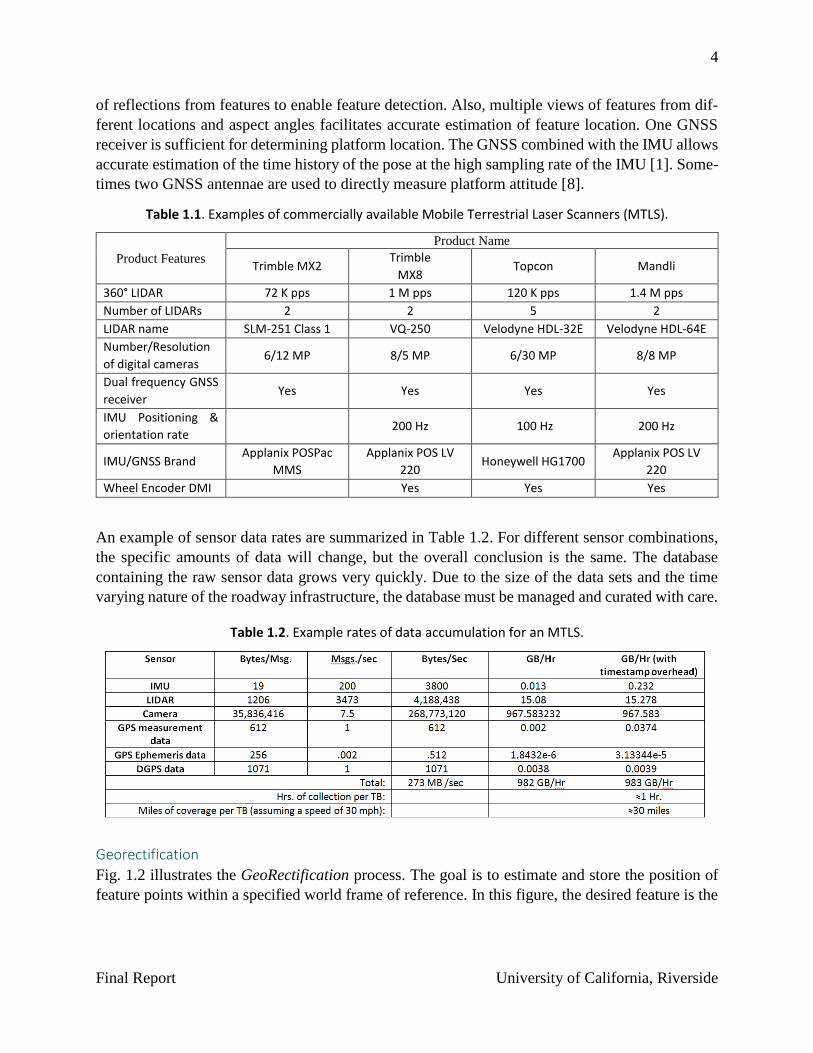
A few examples of sensor packages that are currently available are summarized in Table 1.1. Each
contains at least 6 cameras, providing a nearly 360 degree field-of-view, and at least two LIDAR
sensors. Each contains at least one dual frequency GNSS receiver and an IMU. Multiple cameras
are useful to help ensure that visual imagery is available of the roadway, features, and overhead
structures in spite of occlusions. Multiple LIDAR sensors help to ensure a sufficiently dense set
4
Final Report University of California, Riverside
of reflections from features to enable feature detection. Also, multiple views of features from dif-
ferent locations and aspect angles facilitates accurate estimation of feature location. One GNSS
receiver is sufficient for determining platform location. The GNSS combined with the IMU allows
accurate estimation of the time history of the pose at the high sampling rate of the IMU [1]. Some-
times two GNSS antennae are used to directly measure platform attitude [8].
Table 1.1. Examples of commercially available Mobile Terrestrial Laser Scanners (MTLS).
Product Features
Product Name
Trimble MX2 Trimble
MX8 Topcon Mandli
360° LIDAR 72 K pps 1 M pps 120 K pps 1.4 M pps
Number of LIDARs 2 2 5 2
LIDAR name SLM-251 Class 1 VQ-250 Velodyne HDL-32E Velodyne HDL-64E
Number/Resolution
of digital cameras 6/12 MP 8/5 MP 6/30 MP 8/8 MP
Dual frequency GNSS
receiver Yes Yes Yes Yes
IMU Positioning &
orientation rate 200 Hz 100 Hz 200 Hz
IMU/GNSS Brand Applanix POSPac
MMS
Applanix POS LV
220 Honeywell HG1700
Applanix POS LV
220
Wheel Encoder DMI Yes Yes Yes
An example of sensor data rates are summarized in Table 1.2. For different sensor combinations,
the specific amounts of data will change, but the overall conclusion is the same. The database
containing the raw sensor data grows very quickly. Due to the size of the data sets and the time
varying nature of the roadway infrastructure, the database must be managed and curated with care.
Table 1.2. Example rates of data accumulation for an MTLS.
Georectification
Fig. 1.2 illustrates the GeoRectification process. The goal is to estimate and store the position of
feature points within a specified world frame of reference. In this figure, the desired feature is the

5
Final Report University of California, Riverside
center of the left hand turn sign. The frame of ref-
erence has its origin at the center of the intersec-
tion. This feature position is depicted by the green
arrow, which is indicated by the symbol 𝑃𝐹𝑊for the
position of the feature F relative to the World.
There is no single sensor that can efficiently pro-
vide 𝑃𝐹𝑊, so the vector is instead measured indi-
rectly through the various quantities shown in the
right hand side of the equation at the bottom of the
figure. GNSS and IMU data can be processed to
determine the position and rotation (i.e., the pose)
of the sensor platform relative to the world. This
vector is represented by the purple arrow in the fig-
ure. The position and orientation are represented by the purple symbols 𝑇𝑊𝑃𝑊 and 𝑅𝑊𝑃 in the equa-
tion at the bottom of the figure. The translation and orientation of the LIDAR and Camera frames
relative to the IMU are known and fixed when the platform is designed. These quantities a repre-
sented by the red arrow and the red symbols 𝑇𝑃𝐿𝑃 and 𝑅𝑃𝐿 in the equation at the bottom of the figure.
Finally, the yellow arrow represents the LIDAR measurement of the feature location relative to
the LIDAR frame, which is represented by 𝑃𝐹𝐿. Because all the quantities on the right hand side of
the equation can be computed from the sensor data, the desired position of the feature in the world
frame 𝑃𝐹𝑊, as necessary for a map, can be computed.
Various factors affect the accuracy and success of sensor based mapping. The right-hand side of
the georectification equation in Fig. 1.2 contains five quantities that are estimated from the data.
Any inaccuracies in the determination of these five quantities accumulates into the overall inaccu-
racy of 𝑃𝐹𝑊 . The quality of the IMU, GNSS and processing algorithms determine the accuracy of
𝑇𝑊𝑃𝑊 and 𝑅𝑊𝑃, which are computed at high-rates. Processing algorithms typically smooth IMU and
GNSS data optimally in a post-processing mode [1,9,10,11]. While the quantities 𝑇𝑃𝐿𝑃 and 𝑅𝑃𝐿 are
accurately initialized based on design calculations, their values may also be refined in the post-
processing optimization process. The reliability of detecting features and the accuracy of estima-
tion of 𝑃𝐹𝐿 are determined by various LIDAR and operational issues, predominantly the distribution
and density of LIDAR reflections from the feature’s surface. Various articles discuss the pro-
cessing of LIDAR point clouds to detect roadway relative features [12-20].
Laser Scanning and Photogrammetry: STLS, MTLS, ALS
The principles underlying Laser Scanning and Photogrammetry are similar and will be treated
together in three different scenarios [21]: Stationary Terrestrial Laser Scanning (STLS), Mobile
Terrestrial Laser Scanning (MTLS), and Aerial Laser Scanning (ALS).
Figure 1.2 Georectification Process
6
Final Report University of California, Riverside
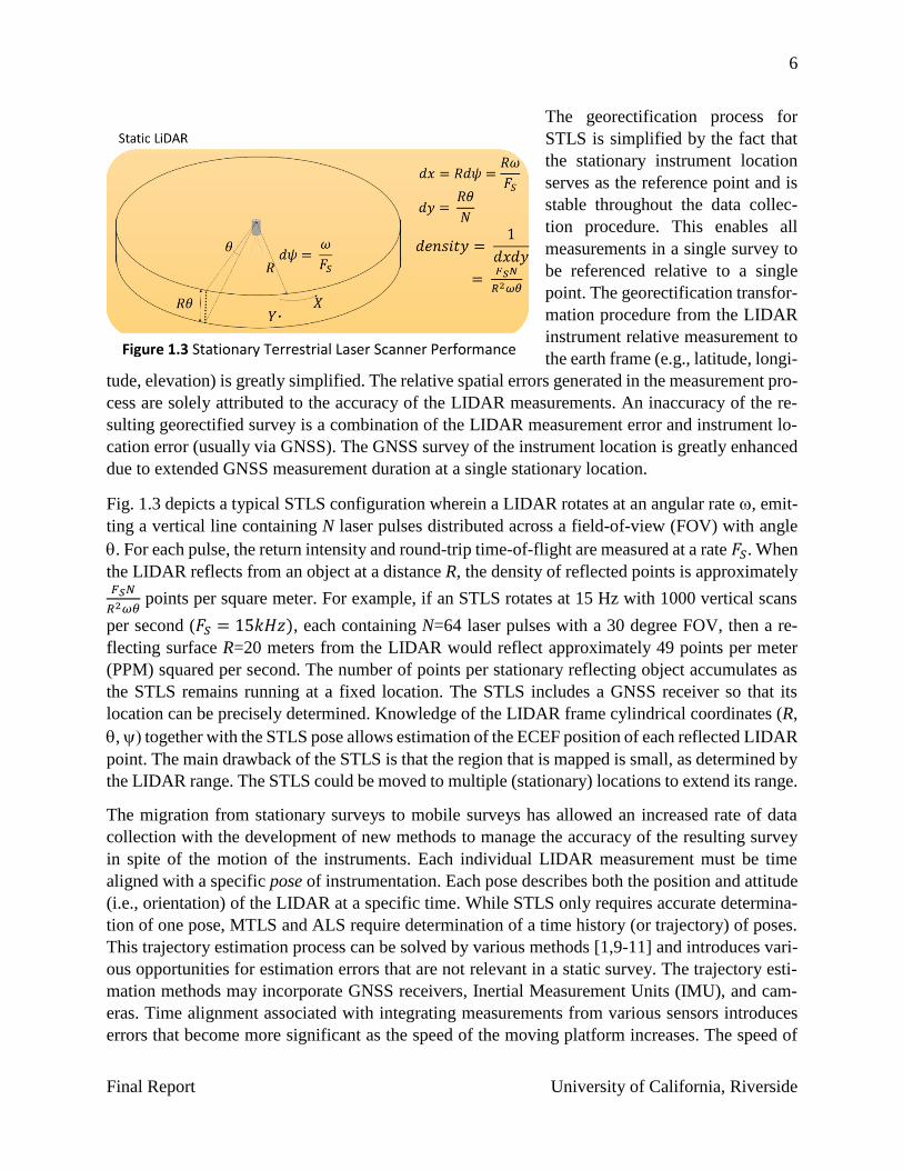
The georectification process for
STLS is simplified by the fact that
the stationary instrument location
serves as the reference point and is
stable throughout the data collec-
tion procedure. This enables all
measurements in a single survey to
be referenced relative to a single
point. The georectification transfor-
mation procedure from the LIDAR
instrument relative measurement to
the earth frame (e.g., latitude, longi-
tude, elevation) is greatly simplified. The relative spatial errors generated in the measurement pro-
cess are solely attributed to the accuracy of the LIDAR measurements. An inaccuracy of the re-
sulting georectified survey is a combination of the LIDAR measurement error and instrument lo-
cation error (usually via GNSS). The GNSS survey of the instrument location is greatly enhanced
due to extended GNSS measurement duration at a single stationary location.
Fig. 1.3 depicts a typical STLS configuration wherein a LIDAR rotates at an angular rate , emit-
ting a vertical line containing N laser pulses distributed across a field-of-view (FOV) with angle
. For each pulse, the return intensity and round-trip time-of-flight are measured at a rate 𝐹𝑆. When
the LIDAR reflects from an object at a distance R, the density of reflected points is approximately 𝐹𝑆𝑁
𝑅2𝜔𝜃 points per square meter. For example, if an STLS rotates at 15 Hz with 1000 vertical scans
per second (𝐹𝑆 = 15𝑘𝐻𝑧), each containing N=64 laser pulses with a 30 degree FOV, then a re-
flecting surface R=20 meters from the LIDAR would reflect approximately 49 points per meter
(PPM) squared per second. The number of points per stationary reflecting object accumulates as
the STLS remains running at a fixed location. The STLS includes a GNSS receiver so that its
location can be precisely determined. Knowledge of the LIDAR frame cylindrical coordinates (R,
, together with the STLS pose allows estimation of the ECEF position of each reflected LIDAR
point. The main drawback of the STLS is that the region that is mapped is small, as determined by
the LIDAR range. The STLS could be moved to multiple (stationary) locations to extend its range.
The migration from stationary surveys to mobile surveys has allowed an increased rate of data
collection with the development of new methods to manage the accuracy of the resulting survey
in spite of the motion of the instruments. Each individual LIDAR measurement must be time
aligned with a specific pose of instrumentation. Each pose describes both the position and attitude
(i.e., orientation) of the LIDAR at a specific time. While STLS only requires accurate determina-
tion of one pose, MTLS and ALS require determination of a time history (or trajectory) of poses.
This trajectory estimation process can be solved by various methods [1,9-11] and introduces vari-
ous opportunities for estimation errors that are not relevant in a static survey. The trajectory esti-
mation methods may incorporate GNSS receivers, Inertial Measurement Units (IMU), and cam-
eras. Time alignment associated with integrating measurements from various sensors introduces
errors that become more significant as the speed of the moving platform increases. The speed of
Figure 1.3 Stationary Terrestrial Laser Scanner Performance
Analysis

7
Final Report University of California, Riverside
the survey platform transitioning through the environment also affects the quantity of data col-
lected for a specific region. The point density in a mobile survey will become sparser as the veloc-
ity of the measurement platform increases.
ALS mounts the sensor platform on either a piloted or autonomous aerial vehicles (UAVs). The
mapping error in an ALS approach is strongly influenced by two factors: the speed of the platform
and the distance of the LIDAR reflections. Traditional ALS vehicles are fixed wing vehicles that
move at high speeds and cannot hover. The high speed lowers the point density per pass over a
given area and makes time alignment more critical. Long range due to high altitude makes platform
attitude estimation more critical. Imaging of surveyed control points on the ground or incorporat-
ing an IMU provides additional measurements to calibrate these error sources.
For fixed wing aircraft the ALS survey accuracy is typically reduced relative to MTLS and STLS.
This issue is overcome in some ALS implementations where the aerial vehicle (e.g., a quadrotor)
is capable of travelling at slow speeds, hovering, and flight at low altitudes.
Fig. 1.4 depicts a traditional ALS configuration
wherein a LIDAR emits a line containing N laser
pulses distributed across a FOV with angle The
LIDAR line scanner is rigidly mounted so that
straight and level flight results in a scan on the
Earth surface, below the plane, perpendicular to
the direction of travel. The lines are generated
and the return intensity and round-trip time-of-
flight are measured at a rate 𝐹𝑆. When the LIDAR
reflects from an object at a vertical distance h, the
density of reflected points is approximately 𝐹𝑆
𝑉ℎ tan (𝜃
𝑁) points per square meter. For example, if
an ALS at traveling at V=100 m/s emits pulses at a line rate of 𝐹𝑆 =15 kHz, with N=64 laser pulses
per line over a 30 degree FOV, then a reflecting surface h=5000m below the LIDAR would reflect
approximately 4 PPM. The number of points per reflecting object does not accumulate, unless the
aircraft traverses the airspace above the reflecting object multiple times. Because the aircraft is
moving, it typically is instrumented with at least one GNSS antenna and receiver and an IMU.
These instruments allow accurate determination of the LIDAR attitude and position at the high
LIDAR sampling rate. The aircraft is typically also instrumented with cameras allowing the detec-
tion of known survey points on the earth for calibration and cross-checking. A main advantage of
ALS is that it can cover a large geographic area much faster that is possible with an STLS. The
main disadvantages are the lower density and position accuracy of the reflected points.
An MTLS mounts one or more rotating LIDARs onboard a land vehicle that can be driven through
the environment to be mapped. The MTLS is more mobile than an STLS allowing it to acquire
data more rapidly for mapping a roadway network. However, reflecting objects may be occluded
Figure 1.4. Aerial Laser Scanner Performance
Analysis

8
Final Report University of California, Riverside
from the LIDAR by interfering entities such as other vehicles. The density of the point cloud along
the roadway is approximately 𝐹𝑆𝑁
𝑅2𝜔𝜃 points per meter. The number of points reflected per object
does accumulate as the MTLS drives by, but only over a short time-window determined by the
speed of travel of the vehicle. Multiple transits within a given section of roadway, although not
required, may have several benefits: increased point cloud density, decreasing the likelihood of
occluded sections, and acquiring surface reflections from various aspect angles.
Tables 1.3 and 1.4 compare the accuracy, collection speed and range of STLS, MTLS, and ALS.
Table 1.3 is qualitative, while Table 1.4 gives example numbers based on assumed experimental
conditions [21]. The point density is critical to the performance of automated feature (e.g., lane
stripe) detection.
Table 1.3. Qualitative comparison of STLS, MTLS, and ALS.
Laser Scanner Stationary Mobile Aerial
Collection Range/ Speed Small Large Very Large
Point Density High Medium Low
Table 1.4. Example quantitative comparison of MTLS and ALS [21].
Laser Scanner Mobile Aerial
Point Density (ppm) 100 - 3000 10-50
Field of View (degree) 360 45-60
Measurement Rate (pps) 160,000 – 400,000 200,000
Relative Accuracy (ft) 0.023 0.065
Absolute Accuracy (ft) Submeter 0.25 – 0.5
The ALS and MTLS instrument suite includes GNSS and IMU to enhance the accuracy of the
platform trajectory (pose history) estimation. The IMU also enhances that ability to accurately time
align the instrument measurements with the appropriate vehicle pose. Commercial trajectory esti-
mation approaches reliably achieve meter level trajectory estimation with the MTLS system mov-
ing at highway speeds. Use of advanced estimation methods has demonstrated decimeter level (or
better) automated survey results [1]. When accuracies equivalent to a stationary survey are re-
quired with a mobile application, individual control points can be surveyed and used to improve
the accuracy of the MTLS survey.
Crowd Sourced Data
Crowd sourced-based mapping data consist of vehicle trajectories from connected vehicles them-
selves, or ordinary from drivers that have navigation software running either through their cellular
phone or through on-board devices typically used for general navigational purposes. These anon-
ymized trajectories provide very large datasets that explicitly contain potentially useful infor-
mation about traffic conditions. The datasets do not contain explicit information about roadway
features such as stop bars or lane edges; however, bundles of closely spaced trajectories provide
useful information about number of lanes, lane centerlines, lane and route connectivity, road con-
ditions, and other items. The individual trajectory data are not highly accurate, because the location
of the data recording device in the vehicle is typically not known and cellphone or on-vehicle
position determination is currently not accurate to more than a few meters. Enhanced processing
9
Final Report University of California, Riverside
algorithms may be able to improve accuracy. Most importantly, the data are timely and low cost,
and can serve complementary purposes to accurate surveyed data sets, as described in Chapter 4.
The data can, for example, detect accidents, pot holes, obstacles, road closures, or newly opened
streets or roadway connections, which could trigger a request for mapping by more accurate means.
The use of crowd-sourced trajectory data for various mapping purposes is a subject of a separate
technical report outside the scope of this project (see [37]).
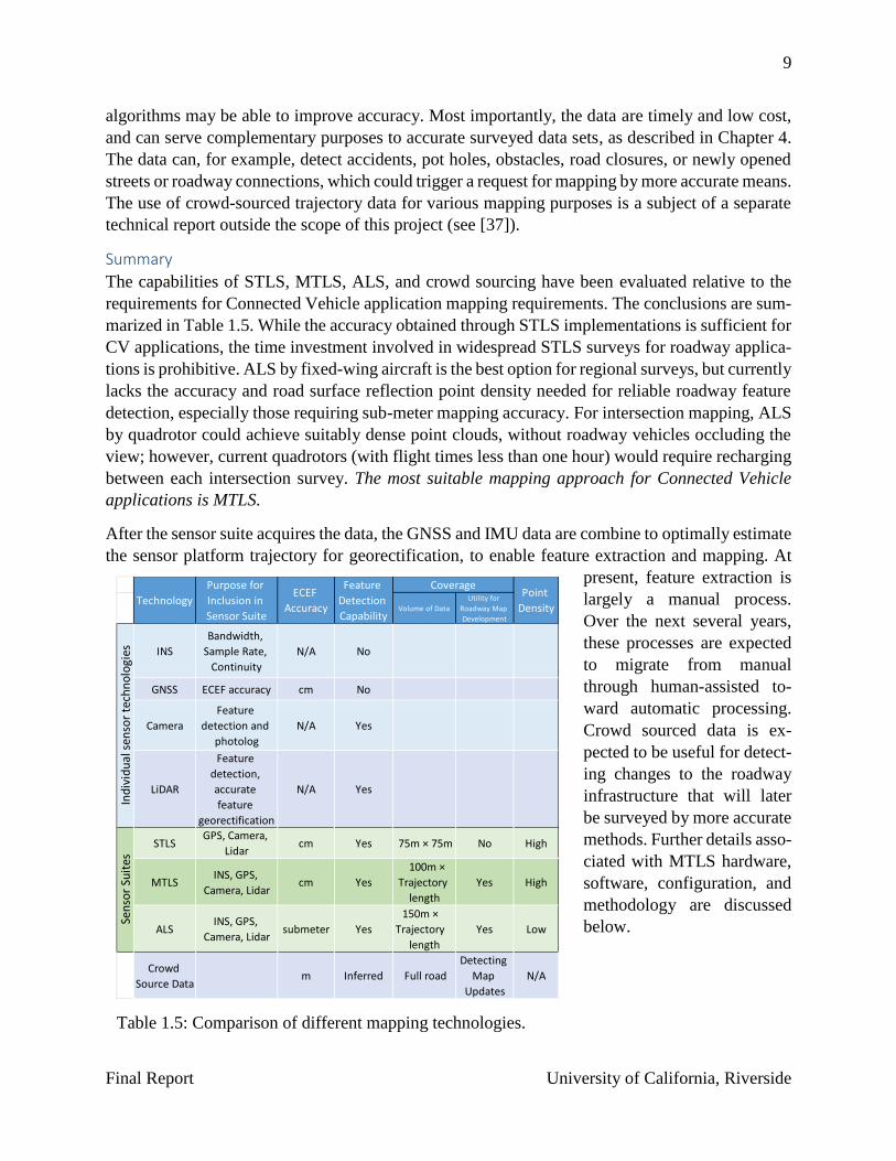
Summary
The capabilities of STLS, MTLS, ALS, and crowd sourcing have been evaluated relative to the
requirements for Connected Vehicle application mapping requirements. The conclusions are sum-
marized in Table 1.5. While the accuracy obtained through STLS implementations is sufficient for
CV applications, the time investment involved in widespread STLS surveys for roadway applica-
tions is prohibitive. ALS by fixed-wing aircraft is the best option for regional surveys, but currently
lacks the accuracy and road surface reflection point density needed for reliable roadway feature
detection, especially those requiring sub-meter mapping accuracy. For intersection mapping, ALS
by quadrotor could achieve suitably dense point clouds, without roadway vehicles occluding the
view; however, current quadrotors (with flight times less than one hour) would require recharging
between each intersection survey. The most suitable mapping approach for Connected Vehicle
applications is MTLS.
After the sensor suite acquires the data, the GNSS and IMU data are combine to optimally estimate
the sensor platform trajectory for georectification, to enable feature extraction and mapping. At
present, feature extraction is
largely a manual process.
Over the next several years,
these processes are expected
to migrate from manual
through human-assisted to-
ward automatic processing.
Crowd sourced data is ex-
pected to be useful for detect-
ing changes to the roadway
infrastructure that will later
be surveyed by more accurate
methods. Further details asso-
ciated with MTLS hardware,
software, configuration, and
methodology are discussed
below.
Table 1.5: Comparison of different mapping technologies.
Volume of Data
Utility for
Roadway Map
Development
INS
Bandwidth,
Sample Rate,
Continuity
N/A No
GNSS ECEF accuracy cm No
Camera
Feature
detection and
photolog
N/A Yes
LiDAR
Feature
detection,
accurate
feature
georectification
N/A Yes
STLSGPS, Camera,
Lidarcm Yes 75m × 75m No High
MTLSINS, GPS,
Camera, Lidarcm Yes
100m ×
Trajectory
length
Yes High
ALSINS, GPS,
Camera, Lidarsubmeter Yes
150m ×
Trajectory
length
Yes Low
Crowd
Source Datam Inferred Full road
Detecting
Map
Updates
N/A
Ind
ivid
ual
sen
sor
tech
no
logi
esSe
nso
r Su
ites
Technology
Feature
Detection
Capability
CoveragePoint
Density
ECEF
Accuracy
Purpose for
Inclusion in
Sensor Suite

10
Final Report University of California, Riverside
1.3 MTLS Process, Instruments, Software
Due to the conclusion of the prior section that MTLS is currently the most appropriate approach
for automated intersection mapping, this section expands on the MTLS process, instruments, and
software processing. MTLS’s are composed of numerous individual sensors mounted upon a sin-
gle platform, as summarized in Table 1.5.
The common sensors and components comprising an MTLS include:
LIDAR(s) – either planar or rotating LIDAR sensor(s)
Camera(s) – one or more cameras
GNSS – Real Time Kinematic (RTK) capable GNSS receiver
IMU – Inertial measurement
Processors – Data logging with precisely time aligned data streams
Data Storage – repository for partially processed data onboard the vehicle
Power support – energy storage and/or generation to handle additional power loads
The physical construction of the MTLS requires significant consideration to physical layout, oc-
clusions, signal processing, calibration, and configuration. Each individual sensor possesses spe-
cific operational constraints and considerations. When properly integrated and configured the sys-
tem provides accurate and robust system for mapping roadway infrastructure effectively and effi-
ciently [2, 22]. The overall process is depicted in Fig. 1.1.
The physical layout attempts to provide a rigid structure, so that the pose variables 𝑇𝑃𝐿𝑃 and 𝑅𝑃𝐿
defined relative to Fig. 2.1 are constant. The camera(s) and LIDAR(s) are mounted to not be oc-
cluded by the mounting structure and the other instruments, while also having a clear view of the
roadway and its environment. It is critical that the LIDAR(s) are able to acquire a high density of
roadway reflections to allow detection and recognition of roadway features.
While the sensor data may be processed in real-time for quality assurance, all the data is saved to
the disk with precise time stamps for post-processing. Accurate time alignment is necessary be-
cause the platform is moving. The georectification process sums three vectors to construct the
desired vector 𝑃𝐹𝑊. Three of the quantities in the georectification formula change with the pose of
the vehicle. Accurate time alignment ensures that the correct set of quantities is estimated and
summed.
The first step of the georectification process is determination of the platform trajectory by use of
the GNSS and IMU data. The (differential) GNSS measurements provide constraints on the vehi-
cle location at the measurement time instants at a low rate (i.e., 1 Hz). The IMU measurements
provide constraints on the platform motion between the GNSS measurement epochs at very high
rates (i.e., >200 Hz). Optimal nonlinear smoothing algorithms [1,9,19] combine these data in a
post-processing operation to estimate the platform trajectory. These algorithms can also incorpo-
rate the LIDAR and Camera measurements. For example reflectors easily detectable by either the
LIDAR or Camera may be placed at surveyed locations to serve as control points. This GNSS/IMU
smoothed result provides the time history of the platform pose at the IMU sample rate which is
necessary to perform LIDAR and camera georectification.

11
Final Report University of California, Riverside
The LIDAR data and camera data are stored onboard. The translation of camera data and LIDAR
data into a georectified point cloud and photolog requires extensive post processing, filtering, and
manipulation. The photolog and colorized point cloud are direct outputs of the georectification
process. Commercial companies (e.g., HERE) will soon stitch the photolog images together into a
continuous panoramic image. In either case, the user can fly though this database seeing and ana-
lyzing the roadway environment.
The georectified LIDAR point cloud data are useful for feature detection and mapping. After data
reduction to a small specific region, the first task is to identify the individual points within the
point cloud subset that are expected to belong to the same surface (e.g., high intensity points lying
on a near horizontal surface). These individual points are processed to remove outliers and used to
estimate the desired characteristics to describe the feature (e.g., location).
The designated features such as lane markings, road edges, stop bars, and intersections can be
identified, characterized and defined. This feature extraction process is specific to the attribute and
requires very specific programming. A high density of LIDAR reflections on the surface of interest
greatly facilitates feature detection and mapping.
The process of creating a georectified photolog is similar to processing the LIDAR data but entails
special image processing steps when transitioning from one survey frame to the next. Each image
will possess a small amount of location measurement error. When two or more images are being
merged the images must be processed and aligned to avoid visual blurring and distortion. This
process is well-documented (see, e.g., [23]) but requires significant processing power as the size
of the images increase. Due to the extensive processing requirements the integrated and georecti-
fied photolog (or panoramic image) is created as a post-processing step.
1.4 Applications: Features and accuracy requirements
Numerous ITS applications have been identified with the potential to improve mobility, safety,
and the environment [24-26]. Connected vehicle technology has been identified as an enabling
technology for many of the identified applications. The V2V and V2I connected vehicle imple-
mentations often require accurate positional information relative to a reference map. The reference
map contains road features, such as, lane markings, stop bars, road edges, turn pockets and inter-
section geometry. The goal of this section is to discuss mapping and real-time positioning tradeoffs
and to characterize the accuracy requirements of a variety of connected vehicle applications. For
a common list of connected vehicle applications, we reference the CVRIA
(http://www.iteris.com/cvria/). The CVRIA CV application list is based on the results of an exten-
sive connected vehicle research program carried out by the USDOT over the last decade.

12
Final Report University of California, Riverside
Mapping and Real-time Positioning Tradeoffs
The Fig. 1.5 illustrates a connected vehicle maneuvering within
a lane near an intersection. Various quantities of interest for the
application – forward distance 𝑠𝐹, left distance 𝑠𝐿, and right
distance 𝑠𝑅 – are illustrated. Each of these quantities is com-
puted in real-time at a high rate by differencing the vehicle po-
sition 𝑝𝑉 with a quantity computed from the map information:
𝑝𝐿, 𝑝𝐹, or 𝑝𝑅. For example, 𝑠𝐹 = 𝑝𝐹 − 𝑝𝑉, each of which is un-
certain, with uncertainty indicated in the figure by the size of
the concentric circles around the point. Therefore, the uncer-
tainty in the computed quantity is related to the uncertainty in
the positions. If we characterize the uncertainty by a standard
deviation, then the equation is
𝜎𝑠𝐹= √(𝜎𝑝𝑉
)2
+ (𝜎𝑝𝐹)
2.
This equation is important as it shows the tradeoff between the accuracy specifications of the map
features denoted by 𝜎𝑝𝐹 and the implied accuracy requirements for real-time positioning (i.e., nav-
igation) denoted by 𝜎𝑝𝑉.
Fig. 1.6 illustrates this tradeoff. Assume that for a given application, the distance to the stop bar
‖𝑠𝐹‖ must be computed with a standard deviation of less than one meter. The outermost curve in
the figure shows the locus of points that satisfy this specification. If for example, the map is
accurate to 10 cm, then real-time vehicle position estimated to 0.99 meter accuracy is sufficient.
However, if the map is only accurate to 0.9m, then the vehicle position must be estimated in real-
time to an accuracy of approximately 40 cm.
sL
sF
sR pR
pF
pV
pL
Figure 1.5 CV application varia-
ble definitions

13
Final Report University of California, Riverside
Connected Vehicle (CV) Application Accuracy Requirements
The CV applications from the CVRIA version 1 are presented in three tables (Table 1.6a-1.6c)
segregated as either a mobility, environmental, or safety application2. In these tables, we also de-
scribe to the best of our analysis the mapping accuracy requirements. Vehicles possessing CV
technology will typically possess a GNSS receiver capable of 2 to 3 meters accuracy in many road
environments. This level of GNSS technology will likely provide sufficient accuracy for applica-
tions requiring “Coarse Positioning” in the following tables. The mobility applications requiring
“Lane Level Positioning” or “Where in Lane Positioning” will require improved positioning tech-
nology (e.g., a GNSS receiver capable of receiving differential corrections, perhaps processing the
carrier phase information) and likely require an accurate reference map of the roadway.
The CV safety applications, as shown in Table 1.6a, identify numerous applications requiring po-
sitioning better than 3 meters. The pure V2V applications that are independent of lane arrangement
do not require a detailed map representation. Alternately the V2V applications such as Intersection
Movement Assist requires detailed knowledge of the intersection geometry and the position of
vehicles within the intersection. This example clearly requires a detailed intersection reference
map as well as accurate vehicle positioning.
The CV mobility applications, as outlined in Table 1.6b, have several V2I implementations that
required accurate knowledge of a vehicle’s position within the roadway, both from a lateral point-
of-view (e.g., lane markings) and a longitudinal point-of-view (e.g., stop bars at intersections).
Examples include: Traffic Signal Priority, Speed Harmonization, and Intermittent Bus Lanes.
2 Please note that the initial mapping and positioning accuracy analysis was carried out on CVRIA version 1; as of
August 3, 2015 CVRIA version 2 has been released, describing an expanded list of CV applications..
Figure 1.6 CV Mapping and positioning
tradeoffs.
14
Final Report University of California, Riverside
These applications must coordinate specific vehicle movements within a lane and require detailed
reference maps in conjunction with accurate vehicle positioning.
Several CV environmental applications, as shown in Table 1.6c, also require accurate map relative
positioning. Eco Approach and Departure, Eco Speed Harmonization, and Eco Transit Signal Pri-
ority all require detailed knowledge of vehicle position within the roadway. It is important to note
that the required positional accuracy for a specific application must consider the additive errors of
vehicle positioning error and map errors. A two meter vehicle positioning error and two meter map
error leads to a potential four meter error in the CV application deployment. Since errors are more
easily controlled during a mapping survey it is important to reduce map errors whenever feasible.
1.5 Applications: Examples
Rather than report explicitly on each application in Table 1.6, we discuss three example applica-
tions below to provide background on the positioning and mapping needs from the areas of safety,
mobility, and the environment.
Safety Application Example – Emergency Electronic Brake Light (EEBL)
The EEBL application enables a vehicle to broadcast a self-generated emergency brake event to
surrounding vehicles. The receiving vehicle determines the relevance of the event and if appropri-
ate provides a warning to the driver in order to avoid a crash. This application improves driver
safety for both the host vehicle and the remote vehicle as seen in Fig. 1.7. The EEBL equipped
braking vehicle (RV) and the EEBL vehicle receiving the message (HV) can interact in numerous
beneficial scenarios. The most beneficial situation in Fig. 1.7 is scenario 4 when a heavy braking
event occurs and the equipped HV can not only avoid impacting the RV but can moderate is own
deceleration rate. The moderation of deceleration by the HV reduces the risk of additional colli-
sions of non-equipped vehicle following the HV. Many potential scenarios exist for the potential
deployment of EEBL with varying levels of technology implementation.
At the simplest EEBL technology level a vehicle can be equipped to sense the distance and decel-
eration rate of a vehicle directly in front of a host vehicle. This can be accomplished without the
need of absolute vehicle position and only requires proximity (e.g. radar, LIDAR, stereo vision
camera) sensing. EEBL applications which only utilize on-board proximity sensors will be limited
to responding only to vehicles directly in front of a host vehicle. Any obstructions will reduce the
effectiveness of the application.
EEBL applications utilizing CV technology will integrate the equipped vehicles’ absolute position
into the EEBL algorithm. When a vehicle’s positional accuracy is “coarse positioning”, the ben-
efits are limited by approximation relative vehicle positioning between equipped vehicles. A hard
braking event can be broadcast to nearby vehicle as a warning, but countermeasures cannot be
fully deployed since vehicle proximity is unknown and the vehicle may be in different lanes.
EEBL applications utilizing “lane level positioning” can improve the fidelity of the application by
limiting warnings to vehicles in the same lane. This greatly improves the effectiveness of the ap-
plication. Finally, “where in lane” positioning provides the greatest benefit to equipped vehicles.
The scenarios shown in Fig. 1.7 can be fully optimized with where in lane positioning. The relative
position between equipped vehicles will be accurately determined even when line-of-sight doesn’t

15
Final Report University of California, Riverside
exist. The EEBL application is particularly useful when there is line of sight obstruction by other
vehicles or poor weather conditions (e.g., fog, heavy rain). Various automotive OEMs have exper-
imented with the EEBL concept.
Figure 1.7 EEBL Safety CVRIA application as envisioned by OEM (Honda).
Mobility Application Example – Cooperative Adaptive Cruise Control (CACC)
The goal of CACC is through partial automation to coordinate the longitudinal motion of a string
of vehicles by utilizing V2V communications in addition to traditional adaptive cruise control
(ACC) systems. There are a wide variety of CACC implementations, but in general CACC imple-
mentations employ the following conditions:
• V2V messages are communicated between leading and following vehicles, and the appli-
cation performs calculations to determine how and if a string can be formed;
• The CACC system provides speed and lane information of surrounding vehicles in order
to efficiently and safely form or decouple platoons of vehicles; and,
• the “groups” of vehicles that are formed are referred to as “strings” rather than “platoons”
of vehicles (strings are sometimes called loosely coupled platoons).
The simplest CACC technology can be deployed with only proximity (e.g. radar, LIDAR, stereo
vision camera) sensing and with significant gaps between the vehicles. This “no-positioning” ver-
sion would not be able to coordinate platoon formation or decoupling. The application would only
be able to loosely keep a group of vehicles traveling a constant speed. More meaningful imple-
mentations of CACC require some level of absolute vehicle positioning.
When a vehicle’s positional accuracy is at “coarse positioning”, the benefits are limited by approx-
imating relative vehicle positions between equipped vehicles. Lateral maneuvers would not be
feasible without the addition of on-board sensors to determine lane markings and nearby vehicle
proximity. When at “Lane Level” positioning accuracy, it is possible to have the application coor-
dinate vehicle strings with formation and de-coupling maneuvers. But to maximize CACC poten-
tial, “where in lane” accuracy is required to manage complex merge and split maneuvers and min-
imize headway within a string. The additional integration of lane keeping can be assisted by on-
Effectiveness
Scenario
1
Scenario
2
Scenario
3
Scenario
4 • Host vehicle gains benefited
as long as the remote braking
vehicle is: Equipped with DSRC
In the same traffic lane
• Effectiveness metrics
examples:• Crash rate
• Crash mitigation rate speed
reduction

16
Final Report University of California, Riverside
board proximity sensing and sub-meter relative position accuracy. Fig. 1.8 depicts a CACC appli-
cation with relevant gap, headway, and vehicle roles.
Figure 1.8 CACC Mobility CVRIA application as deployed in pilot demonstrations.
Environmental Application Example – Eco Approach and Departure (EAD)
An EAD implementation at signalized intersections provides speed advice to the driver of the ve-
hicle traveling through the intersection. Longitudinal control can be carried out by driver using
driver vehicle interface or the longitudinal control can be automated (e.g., see the GlidePath pro-
gram). The speed of the vehicle is managed to pass the next traffic signal on green or to decelerate
to a stop in the most eco-friendly manner. The application also considers a vehicle's acceleration
as it departs from a signalized intersection. An EAD equipped vehicle will be advised to follow a
speed trajectory based on: SPaT data sent from a roadside equipment (RSE) unit to connected
vehicles via V2I communications; Intersection geometry information; signal phase movement in-
formation; and, potential data from nearby vehicles can also be utilized using V2V communica-
tions. Fig. 1.9 shows the current pilot deployment architecture of EAD at signalized intersections.
At the simplest EAD technology can be deployed with “coarse positioning” and serve as a loose
advisory to the driver. The coarse positioning application would lack precision and only provide
limited environmental or fuel improvements. To improve the potential for EAD, a minimum of
“Lane-level” positioning is required with some level of on-board proximity sensors. The proximity
sensors determine the presence of forward vehicles relative to the equipped vehicle. To fully max-
imize the EAD application potential, “where in lane” accuracy is required to manage maneuvers
during congestion and brief signal opportunities. Careful coordination of SPaT, vehicle position,
vehicle speed, and frontal vehicle’s provide the greatest environmental improvements. Fig. 1.10
depicts a EAD application with signal timing scenarios.
Loosely coupled platoon reduce gaps and reaction delays
“Green” lead vehicle maneuvers (e.g.,
vehicle receives eco-speed limits)
“Green” maneuvers to join a loosely coupled platoon

17
Final Report University of California, Riverside
Figure 1.9 EAD Environmental CVRIA application as deployed in pilot demonstrations.
Figure 1.10 EAD signalized intersection timing scenarios.
Source: Noblis, November 2013
Vehicle Equipped with the Eco-Approach and Departure
at Signalized Intersections Application
(CACC capabilities optional)
Traffic Signal Controller with SPaT Interface
Traffic Signal Head
Roadside Equipment Unit
V2I Communications:
SPaT and GID
Messages
V2V Communications:
Basic Safety
Messages
18
Final Report University of California, Riverside
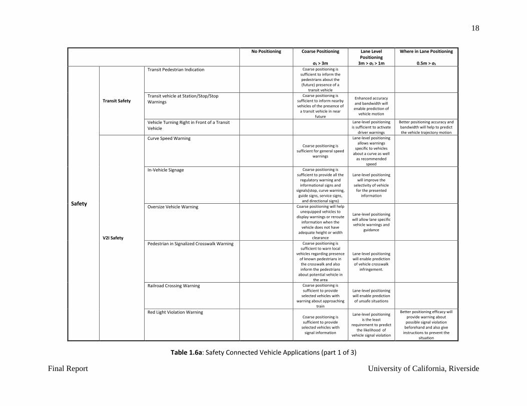
Table 1.6a: Safety Connected Vehicle Applications (part 1 of 3)
No Positioning Coarse Positioning
σS > 3m
Lane Level Positioning
3m > σS > 1m
Where in Lane Positioning
0.5m > σS
Safety
Transit Safety
Transit Pedestrian Indication
Coarse positioning is sufficient to inform the pedestrians about the (future) presence of a
transit vehicle
Transit vehicle at Station/Stop/Stop Warnings
Coarse positioning is sufficient to inform nearby vehicles of the presence of
a transit vehicle in near future
Enhanced accuracy and bandwidth will enable prediction of
vehicle motion
Vehicle Turning Right in Front of a Transit Vehicle
Lane-level positioning is sufficient to activate
driver warnings
Better positioning accuracy and bandwidth will help to predict the vehicle trajectory motion
V2I Safety
Curve Speed Warning
Coarse positioning is
sufficient for general speed warnings
Lane-level positioning allows warnings
specific to vehicles about a curve as well
as recommended speed
In-Vehicle Signage
Coarse positioning is sufficient to provide all the
regulatory warning and informational signs and
signals(stop, curve warning, guide signs, service signs,
and directional signs)
Lane-level positioning will improve the
selectivity of vehicle for the presented
information
Oversize Vehicle Warning
Coarse positioning will help unequipped vehicles to
display warnings or reroute information when the vehicle does not have
adequate height or width clearance
Lane-level positioning will allow lane specific vehicle warnings and
guidance
Pedestrian in Signalized Crosswalk Warning
Coarse positioning is sufficient to warn local
vehicles regarding presence of known pedestrians in the crosswalk and also inform the pedestrians
about potential vehicle in the area
Lane-level positioning will enable prediction of vehicle crosswalk
infringement.
Railroad Crossing Warning
Coarse positioning is sufficient to provide
selected vehicles with warning about approaching
train
Lane-level positioning will enable prediction of unsafe situations
Red Light Violation Warning
Coarse positioning is sufficient to provide
selected vehicles with signal information
Lane-level positioning is the least
requirement to predict the likelihood of
vehicle signal violation
Better positioning efficacy will provide warning about possible signal violation
beforehand and also give instructions to prevent the
situation

19
Final Report University of California, Riverside
Table 1.6a: Safety Connected Vehicle Applications (part 2 of3)
Reduced Speed Zone Warning
Coarse positioning is sufficient
Lane-level positioning allows per lane
guidance
Restricted Lane Warnings
Coarse positioning allows
identical communication to all vehicles
Lane-level positioning allows vehicle specific restriction warnings
and alternative route advice specific to each
lane
Spot Weather Impact Warning
Coarse positioning is necessary to alert drivers about unsafe and blocked
road conditions
Lane specific warning is possible along with
substitute route advice
Automated driver assistance is feasible for local road
conditions
Stop Sign Gap Assist
Lane-level positioning enables warning
drivers on minor roads about unsafe gaps on
the major road
Enhance accuracy improves prediction about possible
collision, especially for multiple vehicles on minor roads
Stop Sign Violation Warning
Lane-level positioning is sufficient to warn
drivers about predicted stop sign
violations
Enhanced accuracy enables automated assistance for better
prediction or prevention
Warnings about Hazards in a Work Zone
Coarse positioning enables warnings about general
hazards (vehicle approaching at high speed) to maintenance personnel
within a work zone
Lane-level accuracy
significantly enhances accuracy of
predictions (giving warnings to more specific vehicles),
reducing false alarms.
Warnings about Upcoming Work Zone
Coarse positioning is sufficient to provide
information about an approaching work zone
condition
Lane-level allows per
vehicle alternate routing suggestions.
V2V Safety
Blind Spot Warning Relative vehicle position is sufficient for applying
currently
Where in lane positioning is necessary when absolute positioning is used in both
vehicles
Control Loss Warning Internal vehicle detection of loss of traction control enables broadcast to all
vehicles within range
Absolute positioning allows far away vehicles to ignore
the message
Allows nearby vehicles to display driver
warnings
Allows automatic vehicle reaction
Do Not Pass Warning
Lane level positioning is necessary to warn about passing zone
which is occupied by vehicles in the
opposite direction of travel
Where in lane will assist drivers regarding when to pass
Emergency Electronic Brake Light No positioning is necessary to broadcast a
self-generated emergency brake event to
surrounding vehicles
Absolute positioning allows far away vehicles to ignore
the message
Allows nearby vehicles to display driver
warnings

20
Final Report University of California, Riverside
Table 1.6a: Safety Connected Vehicle Applications (part 3 of 3)
Emergency Vehicle Alert No positioning is necessary to alert the
driver about the location of and the movement of
public safety vehicles responding to an incident
Absolute positioning allows far away vehicles to ignore
the message
Allows nearby vehicles to display driver
warnings
Forward Collision Warning Relative positioning is
sufficient to implement in current technology
Where in lane positioning is necessary when absolute
positioning is used on both vehicles, plus V2V communications
Motorcycle Approaching Indication Relative positioning can be implemented in today’s
technology to give warnings
Coarse positioning is sufficient for providing
warnings to all the vehicles in specific region
More accurate positioning will
provide more vehicle specific warnings
More accurate positioning will help vehicles to predict any future collision or accident
Intersection Movement Assist
Lane level positioning is necessary to warn
about potential conflicts
Where in lane positioning will improve prediction
Pre-crash Actions
Lane level positioning is necessary to
mitigate the injuries in a crash by activating
pre-crash actions
Where in lane positioning enables faster predictions with
more warning time
Situational Awareness
Coarse positioning is sufficient to broadcast a
general warning to all vehicles about road
conditions measured by other vehicles
Lane level positioning allows more lane
specific warnings, plus vehicles can determine
warning relevance
Slow Vehicle Warning
Coarse positioning is sufficient to warn the
driver about approaching a slow vehicle
Lane level positioning will help providing
warnings to vehicles in specified lane
Stationary Vehicle Warning
Coarse positioning is sufficient to warn the
driver about an approaching stationary
vehicle
Lane specific warnings can be implemented
Tailgating Advisory Relative positioning can be used to provide tailgating
warning with no positioning requirement
Lane level positioning on both vehicles is
necessary in case of absolute positioning
Where in lane will help provide more accurate warnings and
discard the false alarms
Vehicle Emergency Response
Coarse positioning is needed for public safety
vehicles to get information from connected vehicles
involved in a crash
Improved positioning will help to gather more information
Allows diagnosis of how the accident happened

21
Final Report University of California, Riverside
Table 1.6b: Mobility Connected Vehicle Applications (part 1 of 4)
No Positioning Coarse Positioning
σS > 3m
Lane Level Positioning
3m > σS > 1m
Where in Lane Positioning
0.5m > σS
Mobility
Border Border Management Systems No positioning is necessary for electronic
interactions if RF transponder is used
Lane level positioning is necessary when the use of RF transponder
is limited or absent
Commercial Vehicle Fleet Operations
Container Security No positioning is necessary for container
security operation
Container/Chassis Operating Data No positioning is necessary for this
application
Coarse positioning can include more operating
data like route log
Electronic Work Diaries Coarse positioning is necessary to collect
information relevant to the activity of a commercial
vehicle
Better positioning will collect more detailed
work information (routing, log activity,
driving pattern etc.) in future
Intelligent Access Program Coarse positioning is necessary for remote
compliance monitoring
Better positioning will enable more detailed
monitoring
Intelligent Access Program – Mass Monitoring
Commercial Vehicle Roadside Operations
Intelligent Speed Compliance Coarse positioning is necessary for monitoring
speed
Lane level positioning will provide more
information about the driving pattern
Smart Roadside Initiative Coarse positioning is necessary to activate the
application
Lane level positioning will provide more
detailed information
Electronic Payment Electronic Toll Collection No positioning is required when RF
transponder is used to collect tolls electronically and detect and process
violation
Lane level positioning of vehicle is necessary
when the use of RF transponder is limited
or absent
Road Use Charging
Freight Advanced Traveler Information Systems
Freight Drayage Optimization Coarse positioning of the vehicle is necessary for information exchanges
Freight Specific Dynamic Travel Planning Coarse positioning is necessary to have pre-trip
and enroute travel planning, routing, and
other traveler information such as truck parking locations and current
status
Better positioning will help by providing
more detailed route and nearby facility
information in future

22
Final Report University of California, Riverside
Table 1.6b: Mobility Connected Vehicle Applications (part 2 of 4)
Planning and Performance Monitoring
Performance Monitoring and Planning Coarse positioning is necessary to monitor and
collect data including transportation planning,
condition monitoring, safety analyses, and
research and predict speed and travel times
Lane level positioning will predict lane level
speed and travel times and thus improve the application efficiency
Public Safety
Advanced Automatic Crash Notification Relay
Coarse positioning is necessary to automatically
transmit an emergency message in times of crash or other distress situation
Lane level positioning will enable the vehicle to broadcast messages to nearby vehicles only
Emergency Communications and Evacuation
Coarse positioning is sufficient to activate the
application
Incident Scene Pre-Arrival Staging Guidance for Emergency Responders
Coarse positioning is necessary to activate the
application
Incident Scene Work Zone Alerts for Drivers and Workers
Coarse positioning is necessary to activate the
application
Traffic Network Cooperative Adaptive Cruise Control Lane level positioning is sufficient for automatically
synchronizing the movements of many
vehicles within a platoon
Where in lane positioning will improve the applications efficiency and reduce the
occurrences of wanted circumstance
Queue Warning Lane level positioning is sufficient to
broadcast the queued status information
(rapid deceleration, disabled status, lane
location) give warnings to vehicles in
times of potential crash situation
Speed Harmonization Coarse positioning is necessary speed
recommendations based on weather information
Lane level positioning is suitable for speed recommendations
based on traffic conditions

23
Final Report University of California, Riverside
Table 1.6b: Mobility Connected Vehicle Applications (part 3 of 4)
Vehicle Data for Traffic Operations Coarse positioning helps pointing out the changes in
vehicle speeds indicating the disruption of traffic
flow as well as the location of potential incidents
Lane level positioning will help detecting the incident location more
efficiently and accurately
Traffic Signals Emergency Vehicle Preemption Coarse positioning is necessary to activate the
application
Lane level positioning is necessary to plan travelling route and facilitate safe and
efficient movement through intersections
for high priority emergency vehicle
Freight Signal Priority Lane level positioning of freight and
commercial vehicles is necessary to provide traffic signal priority
for traveling in a signalized network
Intelligent Traffic Signal System Lane level positioning of vehicle is necessary to get vehicle location
and movement information to
improve the operations of traffic
signal control systems
Transit Signal Priority Where in lane positioning of transit vehicle is necessary to respond to a transit vehicle
request for a priority at one or a series of intersection
Transit Dynamic Ridesharing Coarse positioning is a necessity to gather
information from both passengers and drivers to
provide them with convenient route by
arranging carpool trips
Better positioning will improve the dynamic
ridesharing application
Dynamic Transit Operations Coarse positioning is necessary to plan,
schedule, modify and dispatch users trips and
itinerary by using automated vehicle location
Better positioning will improve the efficiency
of the application in future
Integrated Multi-Modal Electronic Payment
No positioning is necessary for electronic
interactions if RF transponder is used
Lane level positioning is necessary when the use of RF transponder
is limited or absent

24
Final Report University of California, Riverside
Table 1.6b: Mobility Connected Vehicle Applications (part 4 of 4)
Intermittent Bus Lanes No positioning is necessary to create and
remove a bus lane during peak demand times to
enhance transit operation mobility
Lane level positioning will help maintaining
the lanes
Road ID for the Visually Impaired Coarse positioning is necessary to assist visibly
impaired travelers to identify the appropriate bus and route options to
their intended destination.
Better positioning will help the traveler in
times of distress (road accident, weather
hazard etc.)
Smart Park and Ride System Coarse positioning is sufficient to provide
travelers with real-time information on Park and
Ride capacity
Lane level positioning will provide travelers with the location of
the park and ride capacity
Transit Connection Protection Coarse positioning is necessary to help the
passenger with the information of
approximate arrival time, vehicle transfer to reach safely to the destination
Better positioning will improve the
applications efficiency
Transit Stop Requested Coarse positioning allows a transit passenger to send a
stop request to an approaching transit vehicle
Traveler Information Advanced Traveler Information Systems Coarse positioning is sufficient for the collection
of information including traffic, transit, road
weather, work zone, and connected vehicle related
data
Receive Parking Space Availability and Service Information
Coarse positioning is necessary for providing
pre-trip and enroute traveler information such as truck parking locations
Better positioning will improve the
applications efficiency
Traveler Information-Smart Parking Lane level positioning of the vehicle is
suitable to provide real-time location,
availability, type (e.g., street, garage, AFV
only), and the price of parking

25
Final Report University of California, Riverside
Table 1.6c: Environmental Connected Vehicle Applications (part 1 of 2)
No Positioning Coarse Positioning
σS > 3m
Lane Level Positioning
3m > σS > 1m
Where in Lane Positioning
0.5m > σS
Environmental AERIS/ Sustainable Travel
Connected Eco-Driving Coarse positioning is
required for longitudinal actions such as following
speed advice
Could be necessary to differentiate between lane-based eco-driving
advice
Dynamic Eco-Routing Coarse positioning is
necessary to enable the application
Eco- Approach and Departure at Signalized Intersections
Required for longitudinal speed trajectory planning
Required for differentiating lane-
based SPaT
Required for scenario 3 where vehicle has to stop precisely at
stop bar
Eco-Cooperative Adaptive Cruise Control
Required for lateral and longitudinal
control, with sensor assist
Sensor-based relative positioning is required
Eco-Freight Signal Priority Required for longitudinal speed trajectory planning
Required for differentiating lane-
based SPaT
Eco-Integrated Corridor Management Decision Support System
No positioning is necessary to enable the
application
Coarse positioning provides advanced
functions
Eco-lanes Management Coarse positioning is
necessary to enable the application
Lane level positioning will improve the
application’s efficiency in future
Eco-Multimodal Real-Time Traveler Information
No positioning is necessary to enable the
application
Coarse positioning provides advanced
functions
Eco-Ramp Metering
Lane Level positioning is necessary to
differentiate lane speeds
Eco-Smart Parking Coarse positioning is
necessary to enable the application
Eco-Speed Harmonization Coarse positioning is
necessary to enable the application
Lane level positioning is necessary to
differentiate lane-based speed advice
Eco-Traffic Signal Timing No positioning is
necessary to enable the application
Eco-Transit Signal Priority Required for longitudinal speed trajectory planning
Required for differentiating lane-
based SPaT
Electric Charging Stations Management Coarse positioning is
necessary to enable the application
Low Emissions Zone Management Coarse positioning is
necessary to enable the application

26
Final Report University of California, Riverside
Table 1.6c: Environmental Connected Vehicle Applications (part 2 of 2)
In addition to this CVRIA applications mapping requirements analysis, we also provide an analysis of the requirements of the three
recently initiated Connected Vehicle Pilot Deployment projects in Appendix C.
Roadside Lighting
Coarse positioning is necessary to enable the
application
Road Weather
Enhanced Maintenance Decision Support System
Coarse positioning is
necessary to enable the application
Road Weather Advisories and Warning for Motorists
Coarse positioning is
necessary to enable the application
Possible lane differentiation
required for hazards
Road Weather Information and Routing Support for Emergency Responders
Coarse positioning is
necessary to enable the application
Road Weather Information for Freight Carriers
Coarse positioning is
necessary to enable the application
Road Weather Information for Maintenance and Fleet Management Systems
Coarse positioning is
necessary to enable the application
Variable Speed Limits for Weather-Responsive Traffic Management
Coarse positioning is
necessary to enable the application

27
Final Report University of California, Riverside
1.6 Business Models
The main focus of this Task 1 effort was sensor based mapping approaches and requirements re-
lated to CV applications. Accurate roadway digital databases are also important to other roadway
applications, for example: roadway planning, construction documentation, accident investigation,
roadway inventory assessment, pavement characterization, and vertical clearances. Numerous
sources and methodologies exist to acquire digital roadway infrastructure maps and representa-
tions. The focus thus far has been to explain and analyze the existing technologies, requirements,
and applications. Telephone interviews make clear that the FHWA, state DOT’s and commercial
enterprises are all at various stages of constructing roadway digital data bases.
Before summarizing existing business models, it is useful to consider the issues, tradeoffs, and
desired characteristics related to digital roadway data bases:
Huge data sets: The raw data produced by the instruments is huge. To illustrate the order
of magnitude of data consider the data in Table 1.2: given 4.1 million miles of US public
roads, driven at 50 mph, with 1 TB/hr of data generation, yields about 82x103 TB of raw
data. Much of the data may be irrelevant or redundant. Which raw data should be stored?
How and where should it be stored? Who should have access to it?
Time variation: The roadways, the plates on which they sit, the roadway environment,
and the coordinate systems in which they are defined are all time varying. How often should
the data sets be reacquired? How can obsolete data be detected and removed or replaced?
Database spatial continuity: Connected vehicle commercial success will require uni-
formity of database contents, accuracy, and behavior across geographic boundaries.
Automaker uniformity: Market success will require uniform vehicle behavioral expecta-
tions across auto manufacturers.
State DOTs are required to perform maintenance, management, construction, and oversight of a
state owned roads and highways. This responsibility requires detailed knowledge of the road net-
work, features, attributes, condition, and geometry. The traditional survey methods and photologs
are rapidly being updated with georeferenced GIS databases. When the DOT desires data along an
extensive network, GIS databases are frequently created with data collected through STLS, MTLS,
and ALS. Since the primary interest of state DOTs is the road network, the predominate method
of georeferenced data collection is transitioning toward MTLS mounted on a vehicle and driven
on the state owned roads. The MTLS data collection for state DOTs is either contracted to third
party service providers of MTLS data or state DOTS purchase MTLS equipment and perform their
own georeferenced data collection.
State DOTs that purchase their own hardware and software have the upfront cost for hardware,
software, training, and integration. Once the equipment and methods have been integrated within
the institution there is the incremental cost of performing MTLS based surveys. Software packages
are available to help with data management, georectification, and construction of photologs. This
approach requires highly trained data processing personnel within the DOT are available as con-
sultants. An advantage is that the DOT has complete control of the MTLS equipment and its sched-
ule, plus direct access to the raw and processed to use as is needed. A disadvantage is that the high

28
Final Report University of California, Riverside
quantities of data must be managed and curated. Also, in states where MTLS is performed sepa-
rately by each district, special attention must be paid to combining maps across district boundaries.
Other states contract to third parties (e.g., Mandli) to collect and process the MTLS data. This
shifts the costs of equipment purchase and maintenance, data curation and management, and train-
ing of data processing personnel from the states to the third parties; however, the DOT may be
limited in its access to some forms of data. The third parties try may be able to present the state
DOT’s with a cost savings by more fully utilizing their equipment and expertise, so that their fixed
costs are spread over more projects. Some third parties are working towards automated feature
detection. While the third party is responsible for managing and curating all data from a given
contract period, it may be difficult to combine map information if the state DOT switches between
third party vendors at the end of a contract.
The MTLS generated data is most useful if it can be accessed and used by all knowledgeable
employees of the DOT. Some states and third party providers have developed the expertise to make
this possible through web interfaces.
Finally, if the state DOT’s will be generating the maps for CV applications, those states would
need to specify methods at an early stage to ensure full coverage of all roads, nationwide (or global)
coverage, uniform accuracy, and common interface standards. Without these characteristics, the
automobile manufacturers will not be able to utilize the resulting map databases.
Certain corporate entities are also developing maps intended to have global coverage. Certain cor-
porations (e.g., Apple, Bing, Google) are developing maps intended to be used in consumer appli-
cations (routing, advertising, context based search, autonomous taxi service). Such maps do not
require high-accuracy and do not contain roadway relative features.
Other corporations (HERE, CivilMaps, QUANERGY) are developing highly accurate maps with
global coverage, intending to use a “data as a service” business model.
HERE will have a fleet of over 300 MTLS vehicle allowing them to guarantee a maximum time
between surveys of three years for any road in the U.S., with higher frequency surveys in urban
areas, or surveys on demand in areas that are thought to have changed. Changes are detected using
crowd sourced data or through authorized persons (e.g., DOT employees). They are developing at
least two products of interest:
HERE Reality Lens provides calibrated street-level panoramic views. The user can fly
thorough the roadway environment and perform various types of measurements to support
analysis. This product builds on the EarthMine technology. The database can be accessed
via an internet user interface or downloaded (regionally) to the user computer.
HERE HD Live Map provides a lane-level map with lane edges and centerline. This prod-
uct is intended for connected vehicle and autonomous vehicle type of applications. Point
features can be stored along the lanes. Both real-time and historical traffic information is
expected to be included on a per lane basis.

29
Final Report University of California, Riverside
Both of these products are still under development. HERE is open to discussions about map content
and features, along with contracting options. If they succeed, it would be the first global roadway
map.
There have also been discussions on how the federal government could assist in organizing da-
tasets. Several discussions have been carried out as part of the CVRIA development, and the role
it should play in terms of defining map features and databases.
1.7 Concluding Statement
Connected vehicle applications will continue to improve in performance and feasibility as roadway
feature maps become more accurate and available. The methods and procedures implemented in
the early stages will help define the future needs and requirements. This review and analysis has
characterized the current and existing methods utilized by state DOTs, vendors, and corporations
for collecting and mapping relevant road features and attributes. While most feature extraction and
mapping is currently performed manually, globally applicable feature maps will necessitate that
the processes progress toward human-assisted and eventually to automated processes.

30
Final Report University of California, Riverside
2. MOBILE MAPPING SYSTEM ENHANCEMENTS
2.1 Introduction
Detailed roadway feature maps will need to be developed, maintained, and communicated consist-
ently to support Connected Vehicle (CV) applications. As a result, within the U.S. alone, hundreds
of thousands of intersections and millions of miles of roadway will need to be surveyed, with
application-relevant roadway features mapped to application-specific accuracies. The UC River-
side research team developed a Mobile Positioning and Mapping System (MPMS) platform that
provides an accurate geometric representation of the roadway and relevant roadway features. The
associated data processing interprets the relevant data and provides properties of the roadway and
features in and digitally transmittable map message. Most mapping solutions relevant to the con-
nected vehicle program involve the use of some combination of sensors and equipment, platforms,
processes, and software.
The MMPS is a vehicle mounted technology involving the use of positioning and sensor Global
Position System (GPS) technology, Inertial Measurement Units (IMU), Light Detection and Rang-
ing (LIDAR), and video cameras mounted on vehicles to capture data required for characterizing
roadway geometries as well as the features associated with each roadway. The map data integration
involves the use of input sensor data from multiple sources and the subsequent manipulation, trans-
formation, and integration of the data sources to create new map data that are more accurate, com-
plete, detailed, and current than the individual data sources.
Although certain functions of connected vehicle applications may be performed without requiring
the use of roadway maps, mapping provides some distinct advantages in that it can facilitate the
improvement of positioning accuracy and provide details on roadway features. Connected vehicle
applications use map data to establish vehicle location relative to a map, facilitate positional accu-
racy, and provide data on roadway features over a specified time frame with a level of reliability.
The MPMS is part of a mobile test-bed platform which collects positioning and mapping data from
a variety of sensors and combines them to provide accurate, available and continuous intelligence
on the state of the MPMS moving vehicle and on the surrounding areas, yielding more accurate
and precise location detail and associated feature maps. This current task addresses and details
hardware, software, and configuration enhancements associated with the MMPS to achieve oper-
ational improvements for subsequent tasks.
2.2 Mobile Positioning and Mapping System
The University of California-Riverside’s MPMS mobile test-bed platform collects positioning
and mapping data from a variety of sensors and combines them to provide accurate, continuously
available intelligence about the state of the MPMS and its environment. The system allows cen-
timeter accurate feature maps. The sensor suite includes the following technologies:
LIDAR, Panoramic camera, RADAR: to enable detection of features in platform frame;
GNSS (e.g., GPS): to enable the centimeter accurate estimation of absolute (e.g., ECEF or
state plane) platform position;
High-rate kinematic sensors (e.g., INS): to enable continuous availability and high
time resolution.

31
Final Report University of California, Riverside
This system is mounted on a roadway vehicle which is driven through the environment to capture
roadway data. The UCR MPMS at the start of the project is shown in Fig. 2.1a. The UCR
MPMS at the end of the project is shown in Fig. 2.1b. The purpose of the reconfiguration was to
decrease the extent to which the feature sensors occluded each other. The reconfiguration also
included improvement of the signal and power wiring for the system.
Data captured through the MPMS integrated vehicle telematics is utilized to create a coordi-
nate-based map of features accurately surveyed down to the decimeter level. Such maps are
needed both for CV applications and enabling feature-based sensors to be effectively used as
navigation aids. This mobile mapping can be performed at normal arterial roadway speeds, ena-
bling much faster data collection than what would be possible with conventional surveying tech-
niques. Integration of data from high-rate and aiding sensors increase the accuracy and relia-
bility of sensor fusion algorithms to accommodate asynchronous and latent sensor measure-
ments. This Chapter provides details on the hardware and software improvements implemented to
benefit the subsequent tasks.
2.3 Data Collection Procedure Enhancement
The high-level steps sensor based mapping process is summarized in the Fig. 2.2. The MPMS
platform containing a suite of sensors is placed on the vehicle and moved through the environment
for which a digital map is to be constructed. Sensor data are acquired and processed to produce a
map of roadway features.
A variety of databases are involved in the above steps:
The raw point cloud data set obtained from the LIDAR sensor is usually not distributed
publicly prior to the georectification process, except by special request. Instead, it is main-
tained in a variety of formats within the databases of the entity that acquires the data. The
database formats have been optimized to reduce size and improve handling in post-pro-
cessing steps.
Figure 2.1a: Initial Configuration of UCR MPMS Platform
GPS/IMU
LIDAR
panoramiccamera
Figure 2.1b: Final Platform Configuration of UCR MPMS Platform
GPS Antenna
Color Digital Camera
Hokuyo Planar LiDAR
Delphi ESR ACC Radar
IMU and GPS Receiver
Ladybug Panoramic Camera
Velodyne HDL-64E 3D LiDAR

32
Final Report University of California, Riverside
The raw data from the LIDAR sensor goes through a calibration and georectification pro-
cess which creates a point cloud containing all necessary information for map creation with
high accuracy. The accuracy of the final map representation is highly dependent on the
accuracy of georectification process. Subsequent feature extraction techniques are im-
proved as a result of enhanced calibration and georectification during the data collection
and data processing steps.
A georectified point cloud contains a large amount of redundant information which makes
its use and maintenance difficult and costly. Hence, after manual or automated processing
of the georectified point could data, specific roadway features are extracted along with their
locations and metadata descriptors (these steps are further detailed in Chapter 5) which
remove a large part of redundant information and makes the map representation managea-
ble.
Additional details regarding data calibration and processing are provided below.
Figure 2.2: Data collection and processing flow chart Mobile Positioning Mapping System
Calibration
Prior to the data collection in the field, the MPMS undergoes setup and calibration. The prepara-
tion involves two types of calibration, specifically intrinsic and extrinsic sensor parameter calibra-
tion. Intrinsic sensor parameter calibration involves calibrating the final output according to inter-
nal configuration of the sensor system. Extrinsic sensor calibration involves calibrating the final
output based on the configuration of different sensors relative to each other on the same platform.
To guarantee the accuracy of the final map attributes, the entire system calibration methodology

33
Final Report University of California, Riverside
has been refined, improving sensor alignment and providing measurement parameters established
in a real-world setting.
The MPMS has been transported to a variety of test sites, mounted on a test vehicle, and recali-
brated for procedural validation. Several data collections are then performed in a controlled
environment with known objects to refine the calibration parameters. Following the improved
calibration process, data are collected for comparison purposes. The vehicle with the system is then
driven repeatedly over the test site at different times of the day, with varying levels of congestion.
At the end of each data run, the raw data are examined to determine the data validity which guides
the subsequent data collection process. Once enough data are gathered for a test site, the raw
data collection is complete.
Data Handling
The logged raw data processing has been refined as shown by three major blocks in Fig. 2.3. Raw
GPS, IMU, LIDAR and/or camera measurements are input to the offline processing system. The
data preparation block is the common step for all road feature extraction algorithms. In this block,
the sensor platform trajectory is estimated by smoothing the whole log of GPS and IMU meas-
urements. Subsequently, the raw LIDAR data are calibrated with the factory parameters and con-
verted to global coordinate frame using the optimized vehicle trajectory and extrinsic parame-
ters with respect to IMU, known as the georectification process. Finally, the LIDAR point cloud
is stored into a GIS database. The second block generates the bird’s eye view intensity image of
selected intersection regions and then enhances the intensity image using morphological operations.
In the third block, image processing algorithms are utilized on the intensity image to extract lane
edges and stop bars.
Data Preparation
The LIDAR point cloud is recorded in the reference frame of the LIDAR. The first fundamental
step for all mobile mapping systems is the georectification process, which relies on an accurate estimate
of the position and attitude of the platform trajectory as a function of time. Because the LIDAR is
recording thousands of scans per second and is moving, the platform trajectory is needed at very
high rates. This platform trajectory estimate is obtained by combining the IMU and GPS
data in a post-processing operation referred to as smoothing. The initial condition of
the smoothing process may be the real-time trajectory as obtained from an Extended
Kalman Filter (EKF); however, the post-processed smoothed trajectory will be much
more accurate and reliable. An example smoothed trajectory with accuracy characteri-
zation from [1] is shown in Fig. 2.4.
In the LIDAR preprocessing block of Fig. 2.3, the raw LIDAR measurements are converted to
3D Cartesian coordinates with reference to the LIDAR frame using the calibration parameters and
methods provided by the manufacturer. The 3D coordinates are then passed into the next block to
be transformed to global coordinate frames (i.e., georectification).
The LIDAR points in LIDAR coordinate frame are stored as a list with the time reference when
the laser point detection took place. To convert the LIDAR measurement to global coordinate
frame, we need to find the corresponding vehicle pose at the specific laser detection time.

34
Final Report University of California, Riverside
The pose is obtained by interpolation of the two states in the smoothed trajectory whose times are
closest to the given LIDAR time step. The extrinsic calibration parameters between LIDAR and
body frame must be applied to every data point prior to subsequent processing steps.
Figure 2.3: Data processing flow chart of our LIDAR based Mobile Mapping System
The size of preprocessed data for the 1000 second experiment shown in Fig. 2.4 is about 4
gigabytes. Such datasets hardly fit within standard computer memory. For processing, it is parti-
tioned into 40 megabytes pieces. Each partition is converted to global frame separately, and then
passed into the next processing step. The UCR data storage methodology onboard has been im-
proved to allow for extended data collection events.
The LIDAR dataset in global frame from the previous block is stored in a GIS database. Later
portions of it may be extracted as simple data files, because different applications could imple-
ment different algorithms on these preprocessed data. Instead of using the whole point cloud
database, the feature extraction algorithms usually process only small sections of data to fit within
limited computer memory. The improved partitioning procedure allows for advanced feature ex-
traction as detailed in following tasks.
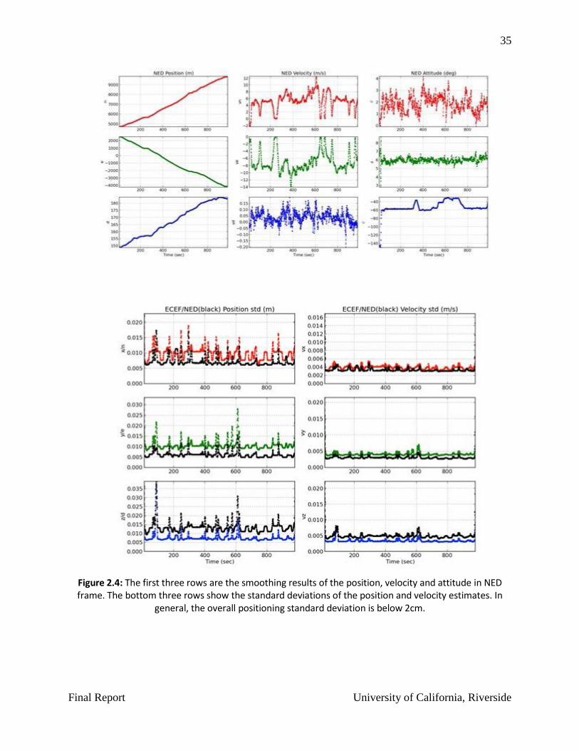
35
Final Report University of California, Riverside
Figure 2.4: The first three rows are the smoothing results of the position, velocity and attitude in NED frame. The bottom three rows show the standard deviations of the position and velocity estimates. In
general, the overall positioning standard deviation is below 2cm.

36
Final Report University of California, Riverside
3. MAP REPRESENTATIONS Detailed roadway feature maps will need to be developed, maintained, and communicated consist-
ently to support Connected Vehicle (CV) applications. As a result, within the U.S. alone, hundreds
of thousands of intersections and millions of miles of roadway will need to be surveyed, with
application-relevant roadway features mapped to application-specific accuracies. Besides con-
nected vehicle applications, accurate roadway digital databases are also important to other road-
way applications such as: roadway planning, construction documentation, accident investigation,
roadway inventory assessment, pavement characterization, and vertical clearances. While many of
these applications have been of interest to Departments of Transportation (DOT’s) for decades,
connected and autonomous vehicles are now bringing these high accuracy maps within the inter-
ests of entities with commercial ambitions, such as auto manufacturers. Successful global com-
mercialization of products incorporating high-accuracy digital maps has created a need for a stand-
ard digital map representation of the road way features and attributes. The digital map representa-
tion should possess the following important characteristics:
- Spatial continuity: Connected vehicle commercial success will require uniformity of da-
tabase contents, accuracy, and behavior across geographic boundaries.
- Automaker uniformity: Connected vehicle market success will require uniform vehicle
behavioral interactions with infrastructure and other vehicles across auto manufacturers.
- Concise and transmittable: Map information should be efficiently and reliably transmit-
table as certain roadway and intersection features must be shared in real-time with vehicles
supporting CV applications.
- Updatable: The roadways, the continental plates on which they sit, the roadway environ-
ment, and the coordinate systems in which they are defined are all time varying. Hence,
roadway maps should be readily updatable.
The automated sensor-based precision mapping process is discussed in Chapter 1. Map updating
will be discussed in Chapter 4.
3.1 Map Representation Approaches
This section reviews various map representations currently known to be available. For successful
collaboration with automakers, it is expected that some entities (government or commercial) will
develop and maintain a continent scale map database, eventually global scale, in some implemen-
tation of a GIS. That GIS maintenance will result in differences between the master GIS and the
maps stored on user vehicles. The master GIS is too large to be convenient for wireless communi-
cation to users in its entirety; therefore, mechanisms have been defined for communication of ap-
plication relevant pieces of the map to connected vehicles.
Geographic Information Systems (GIS)
Geographic information system (GIS) is a system designed to capture, store, manipulate, analyze,
manage, and present all types of spatial or geographical data. ESRI is the dominant supplier of
GIS database, display, management, and analysis tools (e.g., ArcGIS). Such GIS store related data
in layers each of which contains one type of attribute data: street-level data (highways, major roads,
minor roads, one-way arrow indicators, railways), water features, landmarks, building footprints,

37
Final Report University of California, Riverside
administrative boundaries and shaded relief imagery. Even within a single jurisdiction, there may
be many different GIS databases or one combined GIS data base. The GIS itself does not impose
any standardized set of layers nor requirements for accuracy or data representation format for any
given layer. Such standards are determined by outside professional organizations (e.g., SAE, ISO).
As an example, the National Map is a collaborative effort of the United States Geological Survey
(USGS) and other federal, state, and local agencies to improve and deliver topographic information
for the United States. The National Map is part of the USGS National Geospatial Program. The
geographic information available includes orthoimagery (aerial photographs), elevation, geo-
graphic names, hydrography, boundaries, transportation, structures and land cover. The National
Map is accessible via the Web, as products and services, and as downloadable data. Its applications
range from recreation to scientific analysis to emergency response.
Related to transportation, various entities (e.g., federal, state, and regional DOT’s; commercial
entities) maintain their own internal GIS roadway and roadway feature databases. These may be
in unique or proprietary formats, with unique data representations, and entity and geographically
dependent accuracies.
The GIS master roadway map of any of these entities is typically very large, containing the road-
way map for a large region, possibly with underlying raw sensor data, and many features and
attributes necessary for other current and potential applications; therefore, this master GIS is not
concise and transmittable as required for CV applications. Instead, certain portions of the master
GIS are extracted and converted into other formats (e.g., SAE J2735, ISO 14825) that are designed
to be concise and transmittable.
Proprietary Corporate Approaches
There are efforts to develop digital maps with global coverage. Certain corporations (e.g., Apple,
Bing, Google) are developing maps intended to be used in consumer applications (routing, adver-
tising, context based search, autonomous taxi service). Such maps do not require high-accuracy
and do not contain roadway relative features.
Other corporations are developing highly accurate maps specifically intended for consumer and
commercial transportation applications, see Section 1.7.
Corporate entities define proprietary GIS data structures convenient for their internal use and man-
agement. Selected portions of their internal GIS can be export in the pieces and formats (e.g., SAE
J2735) defined by DOT’s and automobile manufacturers for specific applications such as CV’s.
Navigation Data Standard (NDS)
The effort and cost required to maintain proprietary internal GIS formats and convert them to
various customer and application specific standards led a consortium of entities to form of the
Navigation Data Standard (NDS) Association3 in 2006. The Navigation Data Standard (NDS)
3 The members of the NDS consortium as of January 2016 includes at least: Auto Navi, BMW, Bosch, Daimler,
Denso, Garmin, HERE, Hyundai, Mitsubishi Electric, Mxnavi, Nav Info, Panasonic, Tom Tom, Volkswagen, Volvo.

38
Final Report University of California, Riverside
specifies the content (e.g., which items), structure (e.g., how stored), and precision of the physical
format (e.g., SD card) of a map database suitable for automotive applications [5].
The NDS specification includes in its HD model various items useful for Advanced Driver Assis-
tance Systems (ADAS), Connected Vehicles (CV), and Autonomous Vehicles (AV):
High-definition lane models: Store the centerline, boundaries, number of lanes, and at-
tributes (e.g., stop bar, speed limit).
o May be stored as vectors or splines. Current accuracy is at the meter level. Deci-
meter level (5-10 cm) accuracy is desired, as it is expected to be required and suf-
ficient for such advanced applications. Items are stored with centimeter precision.
o Lane connectivity is included, even across intersections, merged lanes, turning
pockets, and stopping lanes.
3d positioning objects: These are items with locations that may be useful for estimating
the position (and state) of a vehicle.
Grade is accounted for as suitable for Eco-driving and EV range conscious routing.
The standard was originally designed for map databases physically stored on the vehicle.
At present, the on-vehicle physical format map is the main approach on which the system will rely.
When there is a communication link, two way communications are possible. Cars could sense the
infrastructure and communicate to a server roadway features that are detected. The cars do not
communicate to each other. The server (i.e. the cloud), after accumulating sufficient confidence,
may alter the map database with such crowd sourced information. The server may communicate
map updates to the vehicles. At present, the methods in this paragraph are not standardized, but
under consideration.
The standard does discuss methods and means for incremental updates. The communication me-
dium is outside the scope of the specification. Whether or not to include a specification for com-
munication of mapping messages is currently under discussion.
Connected Vehicle Standard
Connected vehicle applications expect to communicate map representations for smaller sections
of roadway, via wireless mechanisms, either between vehicles or from the infrastructure to vehi-
cles. This need for transmit-ability, reliability, and accuracy yields a very different set of require-
ments from those for the large internal roadway GIS’s used either statically (without real-time
updates) on a vehicle or within government and commercial entities. These specialized needs for
communicable roadway map pieces have resulted in the SAE J2735 standard that is reviewed next.
At present, the SAE J2735 is the dominant standard intended to CV applications.
BMW, Volkswagen and Daimler (Mercedes) are already offering their infotainment systems with NDS. TomTom and
Nav Info also have NDS products.
Note that the NDS Association is a separate entity from either Society of Automotive Engineers (SAE) or the Inter-
national Standards Organization (ISO).
39
Final Report University of California, Riverside
3.2 SAE J2735
The SAE J2735 standard [6, 28] was designed to enable the mapping needs of CV applications,
within limited communication constraints. SAE J2735 specifies the format by which selected ele-
ments of a larger roadway feature database are communicated between end-users (connected ve-
hicles and infrastructure).
SAE J2735 Message Set Overview
SAE J2735 supports communication of roadway feature and attribute information between vehi-
cles and infrastructure. Typically, the Map GIS is stored on the infrastructure and communicated
to the vehicles, where it is stored and used for some short period of time in support of a CV appli-
cation. For example, in signal, phase, and timing applications, the intersection controller might
broadcast a description of the intersection to all vehicles in the vicinity of the intersection. The
vehicles would maintain that intersection map in their local memory at least until they leave the
vicinity of the intersection.
SAE J2735 Standard specifies a message set, data frames and data elements and is specifically
designed to support applications intended to utilize the 5.9 GHz Dedicated Short Range Commu-
nications for Wireless Access in Vehicular Environments (DSRC/WAVE, referred in this docu-
ment simply as “DSRC”), communications systems [28]. As an example, one of the message sets
that is transmitted from roadway to vehicle includes: current operational status, signal phase and
timing information, intersection geometry, surface conditions, warnings of potential violations or
hazardous conditions, and approaching vehicle information.
The MapData message is used to convey many types of geographic information used in the mes-
sage set. At present, its primary use is to convey one or more intersection lane geometry maps in
a single message. The map message content can include such items as complex intersection de-
scriptions, road segment descriptions, high speed curve outlines (used in curve safety alerts), and
segments of roadway (used in platoon applications).
The MapData message can contain information for up to 32 intersections and 32 roadway seg-
ments. It contains information regarding intersection geometry such as, total number of lanes in
the intersection, lane width, position of the nodes that make up the lanes, position of the stop bar,
crown angle of the road etc. It also contains other attributes like direction of a lane, permitted
maneuvers in a lane, connection to other lanes, lane sharing attributes etc.
The Signal Phase and Timing (SPAT) message communicates dynamic information related to the
map. The SPAT message sends the current movement state of each active phase in the system as
needed (values of what lights are active and values for the current status of the light is expected to
continue). The state of un-active movements (typically all red) is not normally transmitted. Move-
ments are mapped to specific lanes and approaches by use of lane identifiers present in the mes-
sage. These lane identifiers correspond to the specific lanes described in the MAP message for that
intersection. The current signal preemption and priority status values (when present or active) are
also sent.

40
Final Report University of California, Riverside
SAE J2735 Message Set Status
Distribution of such feature maps is still in its infancy. To date, it has not been implemented and
tested over large regions (i.e., states, countries).
To date, various CV testbeds, on increasing size scales have been implemented. As these demon-
strations have progressed recommended changes (e.g., larger sized messages to allow accurate
descriptions of large intersections, additional features) to SAE J2735 have been one of the demon-
stration outcomes.
SAE J2735 Data Structure and Example
Fig. 3.1 illustrates the J2735 data structure and an example drawn on an image of an intersection.
The J2735 is hierarchical. The description of each intersection would contain all of the portions
indicted with colors. The green block describes high-level intersection information: ID, origin and
default lane-width. Lower-level blocks specify the number of lanes followed by descriptions of
each lane, including a lane identifier and a list of nodes along the lane centerline with the first node
on the stopbar. Meta information about the lane can indicate its purpose: ingress, egress, left turn,
etc.

41
Final Report University of California, Riverside
Figure 3.1: J2735 Data Structure and Example.
Orange Node: Intersection center
Red Nodes: Stop bar position
Green Nodes: Ingress node positions
Yellow Nodes: Egress node positions
Black Nodes: Nodes with undecidable
direction
Intersection
ID, center and
lane width
List of lanes
Lane ID,
direction etc.
Lane node
positions
Optional
features
42
Final Report University of California, Riverside
4. MAP REPRESENTATION UPDATING As described in Chapter 3, roadway feature maps are necessary to enable collaboration between
vehicles and with the infrastructure in Connected Vehicle (CV) applications. Therefore, detailed
roadway feature maps will need to be developed, maintained, and communicated consistently. Successful global commercialization of products incorporating high-accuracy digital maps will
require a standard digital map representation of the roadway features and attributes. The roadway
environment is constantly changing based on many factors; in addition, the roadways themselves,
along with the continental plates on which they sit, are also moving. Therefore, in addition to
having spatial continuity across large areas, uniformity between developers/users, and an efficient
data representation, high-accuracy maps databases will need to be updatable. Given the need for
the maps to be updateable, various interesting questions arise:
1) How will the need for local map updates be detected or communicated to the map manager?
2) How will local map updates be integrated into the map database efficiently while maintaining
spatial continuity?
3) How can data integrity be assured if map updates are obtained from different sources?
This section discusses the considerations and methods to address these questions and maintain
maps for utilization in a connected vehicle environment. A suitable approach and methodology is
presented that utilizes data and methodologies currently available.
4.1 Different Methods of Data Collection for Updating
For roadway map-building there are two main methods of information data collection:
Direct – Examples of direct methods include: human surveys, photogrammetry, stationary
terrestrial laser scanning, mobile terrestrial laser scanning, and aerial terrestrial laser scan-
ning. Each of these involves direct detection and calibration of roadway feature locations.
For further detail, see Chapter 1 of this project. Direct methods are performed by trusted
entities either as employees or contractors; therefore, their data have a high-level of integ-
rity and accuracy. These direct methods typically provide the best data, however the data
collection can be expensive and time consuming. Scheduling is either periodic or by re-
quest. These direct methods are typically used by governmental entities and various com-
panies (e.g., Mandli, HERE, CivilMaps).
Indirect (or inferred) – The main example of an indirect method of map data collection is
crowd-sourced data, which for roadway mapping applications refers to the accumulation
of sensor trajectory data from the millions of connected vehicles and/or users driving on
the nations roadways. The “sensors” in this case could be cell phones, navigation sensors
within the vehicle, or standardized Basic Safety Messages (BSMs). This crowd-sourced
method supplies huge quantities of sensor trajectory data from which it may be possible to
mine different types of information about the roadways, such as lane centerlines and inter-
section stop bars. Of particular importance, these crowd-sourced methods can provide data
useful for the prompt detection of changes to the roadway infrastructure. It is important to

43
Final Report University of California, Riverside
note that any map information extracted from crowd-sourcing is inferred, because there is
no direct measurement of the sensor location relative to the roadway features. For example,
tight bundles of similar trajectories might be inferred to represent lanes. Frequent stopping
locations nearest to an intersection ingress point for such a bundle could be inferred to be
a stop bar location. Frequent paths through intersections could be processed to infer in-
gress-egress lane connectivity. Indirect methods can accumulate data rapidly at very low
cost. While the data integrity of each sensor may be suspect, the expectation is that statistics
of the huge data set are very difficult for a small number of users to affect. The potential
limiting factors are that the accuracy of the measured data by the inexpensive user sensors
and validity of the various inferences are uncertain. Crowd-sourced methods have been
investigated by various university research groups and commercial entities, such as,
TomTom Inc.
4.2 Proposed Updating Technique
Experience has demonstrated that these direct and indirect methods are complementary, with each
having a role to play, as depicted in Fig. 4.1. In this figure, the red arrows depict unprocessed
sensor data. When compared to the master roadway GIS database (via the gold arrows), the sensor
data are processed to detect, calibrate and map roadway features and information that can serve as
map updates. These suggested map updates (blue arrows) are recommended to a decision processor
that may make comparisons between the direct and indirect data sources and the master roadway
GIS to determine whether or not to accept the recommendations for incorporation or to schedule a
local survey using direct methods (green arrow). One example is the crowd source data indicating
a connection between two roadways that is not represented in the database, which could automat-
ically trigger a direct survey for that location.
Figure 4.1: Complementary nature of Direct and Indirect map production methods.
Other tasks in this research project describe in detail how the LIDAR-based survey method collects
data, followed by a filtering a feature extraction process. It has been shown how a mapping data
set can be created (e.g., SAE J2735 map standard) going left to right in Fig. 4.1. In addition, crowd-
sourced trajectory data from connected vehicles can be filtered followed by feature extraction,
creating similar map features, as illustrated going right to left in Fig. 4.1. Because these methods
are independent, they can be used for data and map validation, as well as for triggering a need for
updating if the two results do not agree.

44
Final Report University of California, Riverside
5. FEATURE EXTRACTION METHOD
5.1 Introduction
The output of the Mobile Terrestrial Laser Scanning (MTLS) mapping platform is a georectified
3D point cloud of the scanned area which is a set of four dimensional points representing reflection
intensity and centimeter level accuracy Earth-referenced position. Additionally, as a byproduct of
the georectification process the trajectory of the MTLS platform during the data collection process
is available.
The point cloud contains information useful for mapping road features. However, it also contains
large amounts of redundant or non-relevant sensor data. The objective of the feature extraction
task is to extract relevant road feature information from the available MTLS data in a format, such
as the SAE J2735 map message, that is useful for connected vehicle applications. The J2735 map
message is designed for convenience of storage and communication between infrastructure and
users. Such formats include metadata information such as number of lanes and whether lanes are
intersection ingress or egress, which can be extracted from the MTLS platform trajectory data.
Chapter 5 presents the method and results used to extract J2735 map representations from MTLS
data for eleven intersections along the Palo Alto testbed in California. For this study, the features
of interest near intersections include: lane divider markings, road edges, center of intersection, and
stop bars.
Section 5.2 describes this testbed, the data, and data acquisition. Sections 5.3-5.5 describe the data
processing for feature extraction. Chapter 6 will describe the feature extraction results.
5.2 Data
The point cloud data used in this study was collected by the AHMCT research center at UC Davis.
The data were obtained by scanning the California Connected Vehicle testbed on California State
Route 82 (El Camino Real) in Palo Alto. The test bed spans 11 consecutive intersections.
The MTLS includes a Trimble MX8 with two Riegl VQ450 LIDAR scanners, and an Applanix
POS 520 platform positioning system. The left LIDAR has vehicle relative azimuth, roll and pitch
angles of 143, -19 and 23.5 degrees respec-
tively. The LIDAR has vehicle relative azi-
muth, roll and pitch angles of -143, 19 and
23.5 degrees respectively [2]. The platform
mounted on the vehicle is shown in Fig. 5.1.
The platform received corrections from a sin-
gle GNSS base station that used a Trimble R8
receiver located near the testbed. The GNSS
base station location was determined using
NGS OPUS: Online Positioning User Service
and the two hours GNSS base station log data.
Figure 5.1: AHMCT MTLS vehicle.

45
Final Report University of California, Riverside
The testbed contains 11 signalized intersections at the locations listed and as shown in Table 5.1.
The MTLS platform was driven along the ingress and egress sections of the main thoroughfare (El
Camino Real). At each intersection, The MTLS platform was driven along each cross street at least
once. While completing this, the MTLS was driven along each El Camino Real section at least
four times, two northbound and two southbound. The multiple passes along each section provide
a dense points cloud on the surface of the street, which facilitates reliable feature extraction. A
second reason for the multiple passes along a road section is that the effect of dynamic obstructions
(e.g., other vehicles) is unlikely to be the same in the multiple passes, so their effect is a slightly
lower density of returns, instead of the absence of data that would be caused by a single run. The
Table 5.1: Attributes of the testbed intersections
Cross street name Center coordinates Number of points in
million Latitude Longitude
Stanford Ave 37.4277640 122.1492539 77.57
Cambridge Ave 37.4255950 122.1467851 75.36
California Ave 37.4250803 122.1458624 66.03
Page Mill Rd 37.4230638 122.1420467 95.04
Portage Ave/Hansen Way 37.4210617 122.1382334 154.58
Matadero Ave 37.4191602 122.1345428 68.68
Curtner Ave 37.4176288 122.1315912 70.04
Ventura Ave 37.4168366 122.1300875 50.64
Los Robles Ave 37.4157300 122.1281376 70.48
Maybell Ave 37.4120037 122.1246158 59.78
Charleston Ave 37.4104459 122.1233336 83.45
Total Size 871.65
Total Data Size 2559.70
Discarded Points 1688.05

46
Final Report University of California, Riverside
resulting dataset provides both an MTLS georectified point cloud and the trajectory of the plat-
form. The platform trajectory is shown in Fig 5.2a (left). The entire point cloud acquired along this
trajectory contains approximately 2,560 million points.
For each intersection, the J2735 map message requires definition of the intersection center point.
This is a designated reference point that should be near the center and later provided in the J2735
map message. All intersections features described in the J2735 for that intersection will be speci-
fied as offsets relative to the defined center.
Table 5.1 lists the names of the intersection cross streets, the latitude and longitude defined as the
center of the intersection, and the number of points within a radius R=60 meters of the intersection
center. On average each intersection contains around 80 million points on average. Of the 2,560
million points in the full point cloud, approximately 872 million are within the radius R of at least
one of the intersection centers. The remaining 1688 million points are discarded.
5.3 Intersection Feature Extraction Procedure
The full geo-rectified point cloud 𝑃 contains a large number of points obtained while driving the
vehicle along the roadway during the MTLS data acquisition process. To facilitate data processing,
each intersection is processed independently.
The roadway features of interest for this project include lane markings such as lane edges and stop
bars. These features are painted onto the road surface using high-reflectivity paint. The point cloud
Pi for the i-th intersection is designed to contain LIDAR reflection intensity data from which the
desired roadway lane markings and their position information can be extracted. Many other un-
wanted items with high reflectivity also exist within the roadway environment (e.g., signs and
portions of vehicles or buildings). Because the desired lane markings are painted onto the road
surface, many unwanted high reflectivity items can be removed by focusing the feature extraction
process on the road surface; therefore, an important data processing step is to extract the subset of
Pi that contains the road surface. The road surface is modeled as a flat and continuous two-dimen-
sional surface along each ingress or egress portion of an intersection.
The high-level steps in the UCR MTLS roadway feature extraction process can be summarized as
follows.
A. Preprocessing to extract the portions of the point cloud (P) and trajectory (T) relevant to each
intersection. The portion of the point cloud and trajectory relevant to the i-th intersection will
be denoted by 𝑃𝑖 and 𝑇𝑖, respectively.
B. Extraction of road surface point cloud for each intersection. The portion of the point cloud 𝑃𝑖
that corresponds to the road surface of the j-th section of the i-th intersection will be denoted
by 𝑆𝑖𝑗. Additional extracted information from this step includes roadway inner (median) and
outer (curb) edge data that may be extracted during the road surface extraction process. This is
useful as these edges are often not marked with high-reflectance paint and therefore not de-
tectable from the LIDAR intensity data in later steps.
C. Conversion of the intersection road surface point cloud to an image. This step enables use of
image processing tools that are well established and easily available.

47
Final Report University of California, Riverside
D. Image-based roadway feature extraction.
E. Definition of the J2735 feature map for each intersection, including metadata concerning
whether the j-th intersection is an ingress or egress, which is extracted from the trajectory
subset 𝑇𝑖𝑗.
The subsections below provide detailed explanations for input data, output data, and process in-
volved in each high-level step.
Preprocessing to extract Intersection Point Clouds
The accuracy of the geo-rectification process and simplicity of the MTLS data acquisition process
are both enhanced by driving the vehicle through the entire sequence of intersections without turn-
ing off the sensor suite. Also, by leaving the sensor suite turned on while driving between inter-
sections, the data may be useful for multiple purposes besides projects such as this that are mainly
focused on intersections.
The data acquisition process, after geo-rectification provides the point cloud denoted by 𝑃 and
trajectory denoted by 𝑇. The point cloud 𝑃 is too large to process conveniently and contains data
not relevant to the intersections that are of interest. See Fig. 5.2a which shows the trajectory ac-
quired for the Palo Alto corridor. The eleven intersections with centers as defined in Table 5.1 are
marked with circles of radius R. The intersections are ordered with i=1 at the upper left and i=11
at the lower right. The fifth intersection is decomposed into two distinct parts with two centers due
to its unique shape. Fig. 5.2b shows a magnified portion of the trajectories in the vicinity of the
sixth intersection.
To develop a computationally reasonable approach, the first step is to subdivide 𝑃 and 𝑇 into
subsets relevant to each intersection. The center point of the i-th intersection will be denoted as 𝐶𝑖.
These centers are user specified. For the Palto Alto dataset, the values listed in Table 5.1, are
defined within the metadata of the dataset [2]. The user also specifies an intersection radius pa-
rameter R. Given these two parameters, we define for i = 1,…11:
𝑃𝑖 = {x ∈ P | ‖x − C𝑖‖ < R} and 𝑇𝑖 = {x ∈ T | ‖x − C𝑖‖ < R}. (1)
The sets 𝑃𝑖 and 𝑇𝑖 will be processed to extract a J2735 feature map for the i-th intersection. That
process will be repeated eleven times to extract the eleven intersection maps necessary for the Palo
Alto corridor.
Once 𝑃𝑖 and 𝑇𝑖 are defined for all intersection then, the original data sets P and T can be decom-
posed as
𝑃 = ⋃ 𝑃𝑖 + 𝑄11𝑖=1 and 𝑇 = ⋃ 𝑇𝑖 + 𝑈11
𝑖=1 (2)
where 𝑄 and 𝑈 contain point cloud and trajectory data not relevant to the intersections, which will
be ignored in subsequent processing. For the Palo Alto dataset, the quantity of points in each 𝑃𝑖
and in Q is stated in Table 5.1.

48
Final Report University of California, Riverside
Figure 5.2: (a) The platform trajectory data for all 11 intersections. The orange box labeled 1 indicates the
main thoroughfare. Each green circle encloses one intersection. (b) Magnified view of the trajectory
through one intersection, clearly showing multiple traversals of the platform along the main thoroughfair.
To further automate the process in the future, the intersection centers 𝐶𝑖 can be extracted
automatically from the trajectory T or from a network description.
Road Surface Extraction
The inputs for this processing step are the sets 𝑃𝑖 and 𝑇𝑖 defined in eqn. (1) of Section III.A. The
goal of this step is to output a reduced point cloud that only contains those points on the roadway
surface, thereby removing high reflectivity points from extraneous objects (e.g., buildings, vehi-
cles, signs). Each extracted intersection is processed separately, so the process described in this
section is repeated for i = 1, …, 11.
The roadway is modeled as a smooth 2-dimensional surface. This assumption is only locally valid
within each well-defined ingress or egress section of the intersection; therefore, an important step
is to process the intersection trajectory 𝑇𝑖 to extract useful meta-data such as the number of inter-
section components and the direction of traffic flow (i.e., ingress or egress). This metadata will
then be used to divide each 𝑃𝑖 into regions where the 2-dimensional assumption is valid.
The road surface extraction process includes the following steps:
1. Definition of a set of polygons 𝑅𝑖𝑗 each expected to contain the portion of one of the inter-
secting streets from the interior of the intersection to the boundary of 𝑃𝑖;
2. Process the portion of 𝑃𝑖 within 𝑅𝑖𝑗 to extract the road and median edges.
3. Extract point cloud subsets 𝑆𝑖𝑗 for each road segment that only contain points on the road
surface.
Each of these is discussed in the following subsections.
Definition of Intersection Regions
The point cloud 𝑃𝑖 contains many points, only a small percentage of which are on the road surface.
At the start of the processing the only information about the location of the road is the trajectory

49
Final Report University of California, Riverside
𝑇𝑖 and the center location 𝐶𝑖. The initial step uses 𝑇𝑖 to define polygons 𝑅𝑖𝑗 to decompose the point
cloud 𝑃𝑖 into overlapping regions that divide each cross street at the intersection and extend along
that cross street to the boundary of 𝑃𝑖. For a T-intersection this would produce three polygons:
j=1,…,3. For an X-shaped intersection, there would be four regions: j=1,…,4.
Fig. 5.3a shows the extracted trajectory data 𝑇𝑖 for the sixth intersection. The trajectory data is first
rotated to align the main thoroughfare with the horizontal axis, as illustrated in Fig. 5.3b. Next, a
sliding rectangular window, indicated by the yellow box in Fig. 5.3c, is moved vertically from the
bottom to top of 𝑇𝑖 (i.e., from 𝑌𝑚𝑖𝑛 to 𝑌𝑚𝑎𝑥 in Fig. 5.3c). The horizontal width of the trajectory
within that vertical window is recorded as a function of the vertical position, as depicted in Fig.
5.3d. As the sliding window passes through the main thoroughfare, the trajectory width greatly
increases. The values of y at which this widening begins and ends are recorded as 𝑌𝑚𝑖𝑑1 and 𝑌𝑚𝑖𝑑2.
When the sliding window is in the position of 𝑌𝑚𝑖𝑑1 (and 𝑌𝑚𝑖𝑑2), the mean of the horizontal posi-
tion of the trajectory data within that sliding window is defined to be 𝑋𝑝𝑜𝑠1 (and 𝑋𝑝𝑜𝑠2).
The first polygon for the main thoroughfare is defined to contain the corners defined by
(𝑋𝑚𝑖𝑛, 𝑌𝑚𝑖𝑑1), (𝑋𝑚𝑖𝑛, 𝑌𝑚𝑖𝑑2), (𝑋𝑝𝑜𝑠1, 𝑌𝑚𝑖𝑑1) and (𝑋𝑝𝑜𝑠2, 𝑌𝑚𝑖𝑑2). The second polygon for the main
thoroughfare is defined to contain the corners defined by (𝑋𝑚𝑎𝑥, 𝑌𝑚𝑖𝑑1), (𝑋𝑚𝑎𝑥, 𝑌𝑚𝑖𝑑2),
(𝑋𝑝𝑜𝑠1, 𝑌𝑚𝑖𝑑1) and (𝑋𝑝𝑜𝑠2, 𝑌𝑚𝑖𝑑2). The first polygon for the cross street extends vertically between
𝑌𝑚𝑖𝑛 and 𝑌𝑚𝑖𝑑1 with the x-values of the corners defined by the horizontal width of the trajectory
at those y-values. The second polygon for the cross street extends vertically between 𝑌𝑚𝑖𝑑2 and
𝑌𝑚𝑎𝑥 with the x-values of the corners defined by the horizontal width of the trajectory at those y-
values. Each of these corners is expanded horizontally and vertically by a buffer value B=30 me-
ters, because the road surface will be wider that the width defined based on the trajectory 𝑇𝑖. Fig.
5.3e shows the bounding polygons defined for intersection six.
Finally, these polygons are rotated back to the world frame and used to define
𝑃𝑖𝑗
= {(𝑥 ∈ 𝑃𝑖) ⋂(𝑥 ∈ 𝑅𝑖𝑗)}
where 𝑥 ∈ 𝑅𝑖𝑗 is interpreted as the horizontal components of x being in the interior of the polygon.
This segmented intersection can be represented as
𝑃𝑖 = ⋃ 𝑃𝑖𝑗
+ 𝐺
𝐽
𝑗=1
where G contains the elements of the point cloud that are not in any of the J polygons. The points
in G will be ignored after this point. The value of 𝐽 can be 3 or 4 depending on whether the inter-
section is “T” or “X” shaped.

50
Final Report University of California, Riverside
(a) (b)
(c) (d)
(e)
Xpos2
Xpos1
Ymid1
Ymid2
Ymax
Ymin
Ymid2
Ymid1
Main1
side2
side1
Main2
Figure 5.3: (a) Trajectory data Ti for i = 6. (b)
Rotated trajectory data. (c) Process for road
segmentation. (d) Trajectory width as a func-
tion of vertical position. (e) Final output of the
road segmentation process.

51
Final Report University of California, Riverside
Extraction of Road Edges per Section
Given the point cloud subsets 𝑃𝑖𝑗 each containing a segment of an intersecting street, the next step
is to extract the road and median edges for each segment. If any segment does not contain medians,
only road edges are extracted.
For each segment, a one meter wide rectangular window of point cloud data is extracted and pro-
cessed. See Fig. 5.4a. When this rectangle processing is complete, the rectangle slides along the
road segment one meter and the process repeats. Within this narrow window, the road surface is
assumed to be two-dimensional. This assumption is used to detect the road and median edges
within the window. Once these edges are determined, discarding point cloud elements outside the
road edges will automatically remove reflections from roadside entities such as buildings and trees.
Fig. 5.4b shows a sample of the point cloud elements within 𝑃𝑖𝑗 and the sliding rectangle, with
elevation denoted by z plotted versus cross-sectional position denoted by y. The processing records
the mode of the z-value as a function of y. On the road surface, the mode is continuous. At the road
and median edges this function changes abruptly. These abrupt changes are detected by monitoring
both the derivative and inflection points of the curve. The detected points are indicated by red dots
in Fig. 5.4b.
After the road and median edges are extracted for each rectangle, each road and median edge is
processed to remove outliers and insert estimates for missing data items. After that a piecewise
fitting approach is used to fit lines to the road and meridian edge points. Results for one portion of
intersection 6 are shown as red dots in Fig. 5.5. A curve is then defined for each road and median
edge.
After the road edge extraction, points outside the road edges are discarded and the reduced point
cloud
�̅�𝑖𝑗
= {𝑥𝑚 ∈ 𝑃𝑖𝑗|𝑥𝑚 is within the outer edges of the segment}
and the road and median curves are passed to the surface extraction process.

52
Final Report University of California, Riverside
(a) (b)
Figure 5.4: (a) Intersection 6 road segment 𝑃𝑖𝑗. The yellow box depicts the rectangular window that
is slid along the roadway (x- axis). (b) Elevation versus cross-sectional position for points within the
sliding rectangle. Detected road and meridian edge points are marked with red dots.
Figure 5.5: The estimated inner and outer edge points of a road
segment after discarding the outliers and piecewise line fitting.
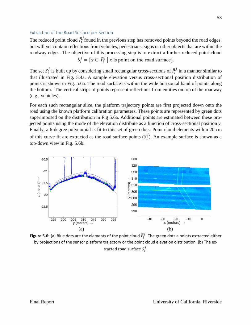
53
Final Report University of California, Riverside
Extraction of the Road Surface per Section
The reduced point cloud �̅�𝑖𝑗found in the previous step has removed points beyond the road edges,
but will yet contain reflections from vehicles, pedestrians, signs or other objects that are within the
roadway edges. The objective of this processing step is to extract a further reduced point cloud
𝑆𝑖𝑗
= {𝑥 ∈ �̅�𝑖𝑗 | 𝑥 is point on the road surface}.
The set 𝑆𝑖𝑗 is built up by considering small rectangular cross-sections of �̅�𝑖
𝑗 in a manner similar to
that illustrated in Fig. 5.4a. A sample elevation versus cross-sectional position distribution of
points is shown in Fig. 5.6a. The road surface is within the wide horizontal band of points along
the bottom. The vertical strips of points represent reflections from entities on top of the roadway
(e.g., vehicles).
For each such rectangular slice, the platform trajectory points are first projected down onto the
road using the known platform calibration parameters. These points are represented by green dots
superimposed on the distribution in Fig 5.6a. Additional points are estimated between these pro-
jected points using the mode of the elevation distribute as a function of cross-sectional position y.
Finally, a 6-degree polynomial is fit to this set of green dots. Point cloud elements within 20 cm
of this curve-fit are extracted as the road surface points (𝑆𝑖𝑗). An example surface is shown as a
top-down view in Fig. 5.6b.
(a) (b)
Figure 5.6: (a) Blue dots are the elements of the point cloud �̅�𝑖𝑗. The green dots a points extracted either
by projections of the sensor platform trajectory or the point cloud elevation distribution. (b) The ex-
tracted road surface 𝑆𝑖𝑗.

54
Final Report University of California, Riverside
Map 3D points to 2D image
The purpose of this step is to convert each road surface point cloud 𝑆𝑖𝑗 into either one or two raster
images, one for each ingress or egress roadway section separated by a median. Many image pro-
cessing tools are available to extract features from such images. This conversion is completed in
the following steps.
First, for roadway segments where Step B detects a median, the median curve is used to divide 𝑆𝑖𝑗
into two separate branches 𝑆𝑖𝑗𝑘
for k=1, 2. If a road segment does not have a median, then the
segment is treated as one branch with k=1.
Second, for each road surface segment branch 𝑆𝑖𝑗𝑘
, points with low reflectivity are removed from
𝑆𝑖𝑗𝑘
to generate a new point cloud subset
𝑆̅𝑖𝑗𝑘
= {𝑥 ∈ 𝑆𝑖𝑗𝑘
| 𝐼(x) > 𝜏}
where is a user defined intensity threshold. A segment before (i.e., 𝑆𝑖𝑗𝑘
) and after (i.e., 𝑆̅𝑖𝑗𝑘
)
intensity thresholding is shown in Figs. 5.7a and 5.7b.
(a) (b)
Figure 5.7: (a) Two branches 𝑆𝑖𝑗𝑘
for k=1, 2 of an extracted road surface segment. (b) Two branches 𝑆̅𝑖𝑗𝑘
for k=1, 2 of an extracted road surface segment after intensity thresholding.
A 2D raster image �̅�𝑖𝑗𝑘
is generated from each point cloud 𝑆̅𝑖𝑗𝑘
. The pixel size of the raster image
in meters is a trade-off between computational complexity and feature position estimation accu-
racy. For the feature extraction approach described herein, each raster pixel is 3 𝑐𝑚 × 3 𝑐𝑚.
Therefore, each raster pixel maps to a 3 cm square cell in the XY region. The value of the pixel
for each cell depends on the elements of 𝑆̅𝑖𝑗𝑘
that map to the cell. When no elements of 𝑆̅𝑖𝑗𝑘
map
to a cell, the pixel value is zero. Otherwise, the pixel value is the average value of the intensities
of the elements of 𝑆̅𝑖𝑗𝑘
that map to the cell. The raster image corresponding to Fig. 5.7 is shown in
Fig. 5.8.
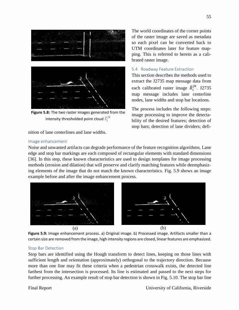
55
Final Report University of California, Riverside
The world coordinates of the corner points
of the raster image are saved as metadata
so each pixel can be converted back to
UTM coordinates later for feature map-
ping. This is referred to herein as a cali-
brated raster image.
5.4 Roadway Feature Extraction
This section describes the methods used to
extract the J2735 map message data from
each calibrated raster image �̅�𝑖𝑗𝑘
. J2735
map message includes lane centerline
nodes, lane widths and stop bar locations.
The process includes the following steps:
image processing to improve the detecta-
bility of the desired features; detection of
stop bars; detection of lane dividers; defi-
nition of lane centerlines and lane widths.
Image enhancement
Noise and unwanted artifacts can degrade performance of the feature recognition algorithms. Lane
edge and stop bar markings are each composed of rectangular elements with standard dimensions
[36]. In this step, these known characteristics are used to design templates for image processing
methods (erosion and dilation) that will preserve and clarify matching features while deemphasiz-
ing elements of the image that do not match the known characteristics. Fig. 5.9 shows an image
example before and after the image enhancement process.
(a)
(b)
Figure 5.9: Image enhancement process. a) Original image. b) Processed image. Artifacts smaller than a
certain size are removed from the image, high intensity regions are closed, linear features are emphasized.
Stop Bar Detection
Stop bars are identified using the Hough transform to detect lines, keeping on those lines with
sufficient length and orientation (approximately) orthogonal to the trajectory direction. Because
more than one line may fit these criteria when a pedestrian crosswalk exists, the detected line
farthest from the intersection is processed. Its line is estimated and passed to the next steps for
further processing. An example result of stop bar detection is shown in Fig. 5.10. The stop bar line
Figure 5.8: The two raster images generated from the
intensity thresholded point cloud 𝑆̅𝑖𝑗𝑘

56
Final Report University of California, Riverside
is shown in red. Other detected lines of sufficient length that are oriented (approximately) orthog-
onal to the lane direction are shown in green.
Figure 5.10: Example of detected stop bar candidates.
Lane Divider Detection
The goal of this step is to divide each branch into lanes. The inputs to this process are the calibrated
raster image �̅�𝑖𝑗𝑘
and the curves defining the road and median edges.
The Hough transform of �̅�𝑖𝑗𝑘
from the previous step also returns lines parallel to the direction of
traffic flow, which are candidates for lane dividers. Good candidates will have sufficient length,
sufficient separation from other lane dividers, and match one of the templates defined in the sub-
sequent sentences. Left turn lanes are frequently set-off by a solid line to their right. On multi-lane
roads, lanes are separated by dashed lines where dashes are 2-3 m long and 4-6 m apart (approxi-
mately) [36].
The software uses a decision tree to process the lines returned by the Hough transform and road
and median edge curves. Depending on the branch width as determined from the median, lane
dividers, and road edge curves, the algorithm labels the branch as a single lane or multi-lane. The
algorithm first checks for solid lines, as used to demarcate turning lanes. The criteria for accepting
solid lines as lane dividers include distance of the line from the branch edges, distance of this line
from already accepted lane edges, line direction and length. After finding solid lines that demarcate
lane edges, the remaining road width is computed, as the basis for a decision concerning the max-
imum number of remaining lanes. Given this estimate of the maximum number of remaining lanes,
the algorithm begins searching through the remaining dashed line checking direction, dash length
and spacing, and separation between previously accepted lane edges and median and road edges.
The process concludes either when the remaining maximum number of remaining lanes is less
than one or when there are no remaining suitable lines to serve as lane dividers. In some cases, for
cross-streets, the branch is too narrow to support multiple lanes and has not lane markings. In this
case, the lane edges are defined to be the road and or median edges. In some cases, such as cross-
streets, the branch has two lanes with no or undetectable markings, yet has width sufficient for two
lanes. In this case, the algorithm defines the curve half way between the branch edges as the lane
separator and processes each lane as a single lane.

57
Final Report University of California, Riverside
Once the lane edges are determined, the lane centerline is computed by dropping nodes midway
between the two lane edges. Nodes are separated by a distance D = 6 m (200 pixels apart). The
first node of the centerline is defined to be at the midpoint of the line segment between the inter-
sections of the lane edges and the stop bar. Lane width is calculated as the inner product of the line
connecting the two points defined by the two lane edges intersecting with the stop bar and the unit
vector that is perpendicular to the lane edge.
Fig. 5.11 illustrates the output of the feature extraction algorithm. The input image �̅�𝑖𝑗𝑘
is the
background. The input road edges are shown as green dotted lines. The extracted stop bar by a
solid yellow line and extracted nodes by blue circles.
Figure 5.11: Output of the feature extraction algorithm.
Challenges
When the road markings are severely faded, the road has no markings, or the input image is very
noisy, the algorithm cannot succeed in its automated processing. In such cases, it generates a warn-
ing and marks the segment for human oversight or intervention. Another issue arises when only
one stop bar is detected, in which case the algorithm proceeds with the detected stop bar and gen-
erates a warning for further human inspection.
Further examples of when such warnings occur are presented in Section IV.
5.5 J2735 Intersection Feature Map Estimation
After the lane centerline nodes and lane widths are estimated, the image coordinates of these nodes
are converted back to UTM coordinates using the metadata saved during raster generation. The
intensity thresholded road surface segments are first rotated back to their original orientation and
then joined together to get an intensity thresholded point cloud 𝑆�̅� for the whole intersection. These
nodes are then superimposed 𝑅𝑖 for analytic comparison.
Top-down view of an intensity thresholded point cloud 𝑆�̅� with the extracted J2735 nodes super-
imposed is shown in Fig. 5.12. According to the specification of the J2735, the first node of each
lane starts from the position of the stop bar which is represented with a red node. The rest of the
nodes in the lane are marked green if it’s a ingress lane and yellow if it’s a egress lane. Sometimes,
in the side road segments, the mapping vehicle did not go through all the lanes; therefore, due to
the absence of a meridian, the algorithm was unable to conclude the direction of travel for those
lane. Those lanes are marked with black nodes. In addition, the nodes coordinates are converted
from UTM to lat-long to superimpose on Google Earth to make a second comparison. The Google
Earth image is shown in Fig. 5.13.

58
Final Report University of California, Riverside
Figure 5.12: Extracted nodes superimposed on the point cloud.
Figure 5.13: Extracted nodes overlaid on google earth.

59
Final Report University of California, Riverside
5.6 Summary of Automation Status
Fig. 5.14 summarizes the automation status of the various processing steps described above. Given
the short (one-year) period of the project, the algorithms that UCR developed focused on “standard
intersections”. These are described by two straight streets intersection at near right angles and
possibly one meridian separating the ingress and egress lanes of each road.
Fig. 5.14 highlights various directions for future work. The automation level of Step 1 might be
enhanced by using existing (low accuracy) roadway network descriptions both to identify to rough
intersection locations and metadata such as the number of ingress and egress lanes per road at each
intersection. The automation level of Step 2 could be generalized to accommodate more general
intersection entities such as pedestrian islands (see example in Fig. 6.4). Step 4 is the fragile step
of the current approach. The comment for Step 5 points to an approach that would automated and
robustify the choice of the intensity threshold and eliminate Step 4 (conversion to an image).
Figure 5.14: Summary of Automation status of the various steps in the process of
generating J2735 intersection maps from MTLS data.
Step Function UCR Automation level Comments
1 PreprocessingGiven a list of intersection locations, the
process is semi-automated.
Most articles in the literature do not describe their
approach to this step.
Segment detection may fail for non-standard
intersections.
2 Road Edge DetectionAutomated for road sections with one curb
and one median, no islands.
3 Road surface extraction Automated
4Mapping of 3D point cloud
to 2D imageSemi-automated
Intensity threshold parameter are tuned for
different road segments.
5Image Enhancement and
Feature ExtractionSemi-automated.
A new graph construction and cutting method
using Otsu's method shows much more
automated performance, combining steps 4 and 5.
6Map message (e.g., J2735)
metadata extraction
Automated for segments with straight lanes.
Semi-automated for non-standard
intersections with curved lanes.
Performance is affected by faded or missing
roadway markings.
7Three dimensional J2735
output with metadataAutomated

60
Final Report University of California, Riverside
6. EXPERIMENTAL RESULTS This section presents the results of applying the method of Chapter 5 to all eleven intersections
along the Palo Alto testbed. Each intersection map is output in the SAE J2735 format.
The J2735 map message includes:
coordinates for the intersection center
the number of lanes
a data structure for each lane including
o a lane identifier
o a sequence of nodes defining the lane centerline
o the lane width
o a point indicating the start of the centerline at the stop bar
o lane attributes such as whether the lane is for ingress or egress.
This project has focused on standard intersections, where essentially orthogonal and straight streets
intersect. The MTLS based approach assumes that the lane markings are clearly painted.
The automated mapping results are illustrated by drawing the J2735 map centerline nodes overlaid
on both the point cloud and a Google Earth image of the intersection. The point cloud data acqui-
sition process includes surveyed control points such that the point cloud has a known accuracy at
the centimeter level [2]. The J2735 overlaid on the point cloud allows evaluation of the absolute
accuracy of the J2735 intersection map. The J2735 overlaid on the Google Earth image gives a
visually interpretable result. The Google Earth imagery is only accurate to 2-5 meters [33, 34, 35].
Therefore, in some instances the entire J2735 overlay is offset relative to the Google Earth image
while aligning well with the point cloud. Such images clearly show the lesser accuracy of the
Google Earth imagery relative to the point cloud. The visual overlay of the J2735 onto the Google
Earth imagery is useful for detecting relative errors between portions of the J2735, for example a
stop bar at the wrong location.
Most of the intersections process completely with correct outputs. In cases where the road mark-
ings are severely faded, the road has no markings, or the input image is very noisy the algorithm
generates a warning and marks the segment for human processing. Another issue arises when only
one stop bar is detected, in which case the algorithm proceeds with the detected stop bar and gen-
erates a warning for further human inspection. In case no stop bar is detected and the algorithm
generates a warning. For these cases, in our results, a stop bar is added manually so the algorithm
can perform the rest of the tasks. The discussion will point out any known processing issues or
errors.
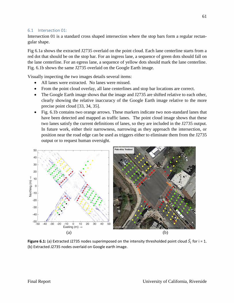
61
Final Report University of California, Riverside
6.1 Intersection 01:
Intersection 01 is a standard cross shaped intersection where the stop bars form a regular rectan-
gular shape.
Fig 6.1a shows the extracted J2735 overlaid on the point cloud. Each lane centerline starts from a
red dot that should be on the stop bar. For an ingress lane, a sequence of green dots should fall on
the lane centerline. For an egress lane, a sequence of yellow dots should mark the lane centerline.
Fig. 6.1b shows the same J2735 overlaid on the Google Earth image.
Visually inspecting the two images details several items:
All lanes were extracted. No lanes were missed.
From the point cloud overlay, all lane centerlines and stop bar locations are correct.
The Google Earth image shows that the image and J2735 are shifted relative to each other,
clearly showing the relative inaccuracy of the Google Earth image relative to the more
precise point cloud [33, 34, 35].
Fig. 6.1b contains two orange arrows. These markers indicate two non-standard lanes that
have been detected and mapped as traffic lanes. The point cloud image shows that these
two lanes satisfy the current definitions of lanes, so they are included in the J2735 output.
In future work, either their narrowness, narrowing as they approach the intersection, or
position near the road edge can be used as triggers either to eliminate them from the J2735
output or to request human oversight.
(a) (b)
Figure 6.1: (a) Extracted J2735 nodes superimposed on the intensity thresholded point cloud 𝑆�̅� for i = 1.
(b) Extracted J2735 nodes overlaid on Google earth image.

62
Final Report University of California, Riverside
6.2 Intersection 02:
This is an almost regular shaped intersection. The main thoroughfare is slightly curved and the
intersecting streets not quite orthogonal, yet the approach worked well.
Fig. 6.2a shows the extracted J2735 overlaid on the point cloud. Each lane centerline starts from a
red dot that should be on the stop bar. For an ingress lane, a sequence of green dots should fall on
the lane centerline. For an egress lane, a sequence of yellow dots should mark the lane centerline.
Fig. 6.2b shows the same J2735 overlaid on the Google Earth image
Visually inspecting the two images details several items:
All lanes were extracted. No lanes were missed.
From the point cloud overlay, all lane centerline locations are correct.
The Google Earth image shows that the image and J2735 are shifted relative to each other,
such that the J2735 centerlines sit on the paint stripes. This clearly showing the relative
inaccuracy of the Google Earth image relative to the point cloud [33,34,35].
Fig. 6.2b has two orange arrows. These markers point to two J2735 stop bar locations
which have been detected and mapped at the wrong line of the pedestrian cross walk. For
the arrow at the lower left, the error is due to worn lane markings. In future work, this issue
could be detected by the fact that stop bar location discontinuously changes from the in-
gress and egress portions of that road segment.
(a) (b)
Figure 6.2: (a) Extracted J2735 nodes superimposed on the intensity thresholded point cloud 𝑆�̅� for i = 2.
(b) Extracted J2735 nodes overlaid on Google earth image.

63
Final Report University of California, Riverside
6.3 Intersection 03:
Intersection 03 is a regular rectangular shaped intersection.
Fig. 6.3a shows the extracted J2735 overlaid on the point cloud. Each lane centerline starts from a
red dot that should be on the stop bar. For an ingress lane, a sequence of green dots should fall on
the lane centerline. For an egress lane, a sequence of yellow dots should mark the lane centerline.
Fig. 6.3b shows the same J2735 overlaid on the Google Earth image.
Visually inspecting the two images details several items:
All lanes were extracted. No lanes were missed.
From the point cloud overlay, all lane centerline locations are correct.
The Google Earth image and J2735 are well aligned.
Note in the Google Earth image that the upper half of the cross street appears to be newly
paved without any lane striping. The point cloud image indicates high intensity lines, so
we suspect that the point cloud was acquired prior to the street being repaved. The mapping
process worked well. This bullet clarifies why no lane striping is visible on this road seg-
ment.
(a) (b)
Figure 6.3: (a) Extracted J2735 nodes superimposed on the intensity thresholded point cloud 𝑆�̅� for i = 3.
(b) Extracted J2735 nodes overlaid on Google earth image.

64
Final Report University of California, Riverside
6.4 Intersection 04:
Intersection 04 is an irregularly shaped intersection that has one side road with a dedicated right-
turn lane with an extra stop bar (see box 1 in Fig. 6.4b), wide side roads with medians, and faded
paintings.
Fig. 6.4a shows the extracted J2735 overlaid on the point cloud. Each lane centerline starts from a
red dot that should be on the stop bar. For an ingress lane, a sequence of green dots should fall on
the lane centerline. For an egress lane, a sequence of yellow dots should mark the lane centerline.
Fig. 6.4b shows the same J2735 overlaid on the Google Earth image.
Visually inspecting the two images details the following items:
The region indicated by the brown and red boxes could not be processed due to the non-
standard road geometry and faded lane striping.
For other road segments the detection of centerline nodes of every lane in all the ingress
and egress branches and the position of the stop bars are estimated correctly.
(a) (b)
Figure 6.4: (a) Extracted J2735 nodes superimposed on the intensity thresholded point cloud 𝑆�̅� for i = 4.
(b) Extracted J2735 nodes overlaid on Google earth image.

65
Final Report University of California, Riverside
6.5 Intersection 05:
Intersection 05 has two T-shaped intersections in close proximity. See Figs. 6.5 and 6.6. Due to
this special structure we decomposed the intersection into intersections 5a and 5b, which are each
much closer to being standard. Each is processed separately.
Intersection 5(a): It is a T-shaped intersection with three road segments. Fig. 6.5a shows the ex-
tracted J2735 overlaid on the point cloud. Each lane centerline starts from a red dot that should be
on the stop bar. For an ingress lane, a sequence of green dots should fall on the lane centerline. For
an egress lane, a sequence of yellow dots should mark the lane centerline. Fig. 6.5b shows the
same J2735 overlaid on the Google Earth image.
Visually inspecting the two images details several items:
There are no stop bar markings on the pavement at the egress section marked as item 1 in
Fig. 6.5b. Given this situation, this system generated a warning to the human operator for
inspection. To proceed, the human manually extends the stop bar line from the parallel
ingress section.
With the manually inserted stop bar, all roadway feature nodes (i.e., centerline and stop bar
nodes in every ingress and egress section) have been detected and mapped correctly. The
stop bar nodes extracted from the manually inserted stop bar are marked with orange.
Note that the stop bar of the left segment of the main thoroughfare (i.e., item 2) is not a
straight line; nonetheless, all the stop bar positions have been correctly detected.
In future work, the insertion of stop bars could be automated, for the cases where the pavement is
unmarked. It is still recommended that the human be alerted, for verification, since this extrapola-
tion of information may not be applicable in non-standard situations. The item 2 in Fig. 6.5b is an
example of a non-standard situation where extending the stop bar between roadway sections would
be inappropriate.
(a) (b)
Figure 6.5: (a) Extracted J2735 nodes superimposed on the intensity thresholded point cloud 𝑆�̅� for i = 5a.
(b) Extracted J2735 nodes overlaid on Google earth image.

66
Final Report University of California, Riverside
Intersection 5(b): It is a non-standard T-shaped intersection with three road segments. The side
road has two dedicated lanes for ingress and egress with extra stop bars (marked in Fig. 6.6b as
items 2 and 3). Along with that structural ambiguity there is an egress segment of the main thor-
oughfare without a painted stop bar (see item 1 in Fig. 6.6b).
Fig. 6.6a shows the extracted J2735 overlaid on the point cloud. Each lane centerline starts from a
red dot that should be on the stop bar. For an ingress lane, a sequence of green dots should fall on
the lane centerline. For an egress lane, a sequence of yellow dots should mark the lane centerline.
Fig. 6.6b shows the same J2735 overlaid on the Google Earth image.
Visually inspecting the two images details several items:
At the egress to the main thoroughfare indicated as item 1, there is no painted stop bar on
the road surface. In this case, the program alerts the user, who manually extends the line
from the parallel ingress lane so that the stop bar definition can be completed.
Items 2-5 all relate to the non-standard structure of the intersection. The current software
is not written to accommodate the curved lane marked by items 4-5 nor the extra stop bars
indicated by items 2-3.
Other than the exceptions note above, the stop bars and centerline nodes of all lanes of both
ingress and egress have been identified correctly.
In future work, the insertion of stop bars could be automated, for the cases where the pavement
is unmarked. It is still recommended that the human be alerted, for verification, since this ex-
trapolation of information may not be applicable in non-standard situations. It is also expected
that the curved right-hand turn lanes can be incorporated into the automated process.
(a) (b)
Figure 6.6: (a) Extracted J2735 nodes superimposed on the intensity thresholded point cloud 𝑆�̅� for i = 5b.
(b) Extracted J2735 nodes overlaid on Google earth image.

67
Final Report University of California, Riverside
6.6 Intersection 06:
This is a non-standard cross-shaped intersection. Note that the cross street sections are off-set lat-
erally relative to each other and the stop bar indicated as item 1 is not orthogonal to the lane cen-
terline and not a straight-line across the entire road.
Fig. 6.7a shows the extracted J2735 overlaid on the point cloud. Each lane centerline starts from a
red dot that should be on the stop bar. For an ingress lane, a sequence of green dots should fall on
the lane centerline. For an egress lane, a sequence of yellow dots should mark the lane centerline.
Fig. 6.7b shows the same J2735 overlaid on the Google Earth image.
Visually inspecting the two images details several items:
Despite its nonstandard aspects all the lanes of every egress and ingress section have been
correctly extracted.
The lane striping is barely visible on the google image.
All the centerline nodes of every lane have been identified correctly.
All the stop bars are positioned correctly except for one side road segment part (indicated
in Fig. 6.7b as item 2).
The misplaced stop bar is expected to be fixable in future efforts.
(a) (b)
Figure 6.7: (a) Extracted J2735 nodes superimposed on the intensity thresholded point cloud 𝑆�̅� for i = 6.
(b) Extracted J2735 nodes overlaid on Google earth image.

68
Final Report University of California, Riverside
6.7 Intersection 07:
This is a standard T-shaped intersection with three road segments.
Fig. 6.8a shows the extracted J2735 overlaid on the point cloud. Each lane centerline starts from a
red dot that should be on the stop bar. For an ingress lane, a sequence of green dots should fall on
the lane centerline. For an egress lane, a sequence of yellow dots should mark the lane centerline.
Fig. 6.8b shows the same J2735 overlaid on the Google Earth image.
Visually inspecting the two images details several items:
All lanes were extracted. No lanes were missed.
All centerlines are correct.
Box 1 shows misplacement of stop bar at an ingress branch of the main road.
Box 2 indicates a main thoroughfare egress where there is no painted stop bar. In this case,
the program alerts the user, who manually extends the line from the parallel ingress lane
so that the stop bar definition can be completed.
The issues pointed to by boxes 1 and 2 could both be addressed in future work.
(a) (b)
Figure 6.8: (a) Extracted J2735 nodes superimposed on the intensity thresholded point cloud 𝑆�̅� for i = 7.
(b) Extracted J2735 nodes overlaid on Google earth image.

69
Final Report University of California, Riverside
6.8 Intersection 08:
This is a standard T-shaped intersection.
Fig. 6.9a shows the extracted J2735 overlaid on the point cloud. Each lane centerline starts from a
red dot that should be on the stop bar. For an ingress lane, a sequence of green dots should fall on
the lane centerline. For an egress lane, a sequence of yellow dots should mark the lane centerline.
Fig. 6.9b shows the same J2735 overlaid on the Google Earth image.
Visually inspecting the two images details several items:
The number of lanes, lane centerlines, and lane widths in every ingress and egress branch
are extracted correctly. No lanes were missed.
Box 1 points to a main thoroughfare egress section for which there is no stop bar painted
on the road surface. This is clear in the point cloud image. The Google Earth image appears
to show a stop bar; however, more careful observation shows that this is an overhead traffic
signal and its shadow on the road surface. The absence of the painted stop bar on the road
surface causes the automatic processing to end with an alert to the user. The user then
manually extends the line of the stop bar from the parallel ingress road section to allow
definition of the J2735 stop bar for each egress lane.
With human interaction for the stop bar at the single egress section, correct extraction and
placement of all stop bars and lane centerline nodes has been achieved.
In future work, the insertion of stop bars could be automated, for the cases where the pavement is
unmarked. It is still recommended that the human be alerted, for verification, since this extrapola-
tion of information may not be applicable in non-standard situations.
(a) (b)
Figure 6.9: (a) Extracted J2735 nodes superimposed on the intensity thresholded point cloud 𝑆�̅� for i = 8.
(b) Extracted J2735 nodes overlaid on Google earth image.

70
Final Report University of California, Riverside
6.9 Intersection 09:
Intersection 09 is an irregularly shaped intersection with one curved and two merging road seg-
ments.
Fig. 6.10a shows the extracted J2735 overlaid on the point cloud. Each lane centerline starts from
a red dot that should be on the stop bar. For an ingress lane, a sequence of green dots should fall
on the lane centerline. For an egress lane, a sequence of yellow dots should mark the lane center-
line. Fig. 6.10b shows the same J2735 overlaid on the Google Earth image.
Visually inspecting the two images details several items:
The two brown boxes mark two road segments that cannot be processed due to irregular
geometric structure and light paint markings. The irregular structure prevents segmenta-
tion, therefore, the remainder of the feature extraction process cannot complete for those
segments of the intersection.
The experiment operated successfully on all the regular shaped road segments with all cen-
terlines mapped identified correctly.
The orange arrow marked box 1 indicates the misplacement of the stop bar of the ingress
branch of the main road segment.
Improvement of the segmentation process for non-standard intersections is a topic for future work.
(a) (b)
Figure 6.10: (a) Extracted J2735 nodes superimposed on the intensity thresholded point cloud 𝑆�̅� for i =9.
(b) Extracted J2735 nodes overlaid on Google earth image.
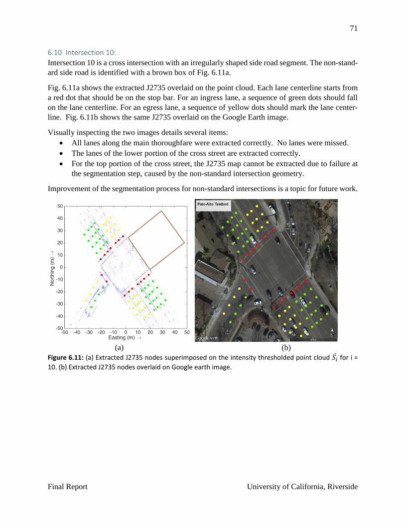
71
Final Report University of California, Riverside
6.10 Intersection 10:
Intersection 10 is a cross intersection with an irregularly shaped side road segment. The non-stand-
ard side road is identified with a brown box of Fig. 6.11a.
Fig. 6.11a shows the extracted J2735 overlaid on the point cloud. Each lane centerline starts from
a red dot that should be on the stop bar. For an ingress lane, a sequence of green dots should fall
on the lane centerline. For an egress lane, a sequence of yellow dots should mark the lane center-
line. Fig. 6.11b shows the same J2735 overlaid on the Google Earth image.
Visually inspecting the two images details several items:
All lanes along the main thoroughfare were extracted correctly. No lanes were missed.
The lanes of the lower portion of the cross street are extracted correctly.
For the top portion of the cross street, the J2735 map cannot be extracted due to failure at
the segmentation step, caused by the non-standard intersection geometry.
Improvement of the segmentation process for non-standard intersections is a topic for future work.
(a) (b)
Figure 6.11: (a) Extracted J2735 nodes superimposed on the intensity thresholded point cloud 𝑆�̅� for i =
10. (b) Extracted J2735 nodes overlaid on Google earth image.
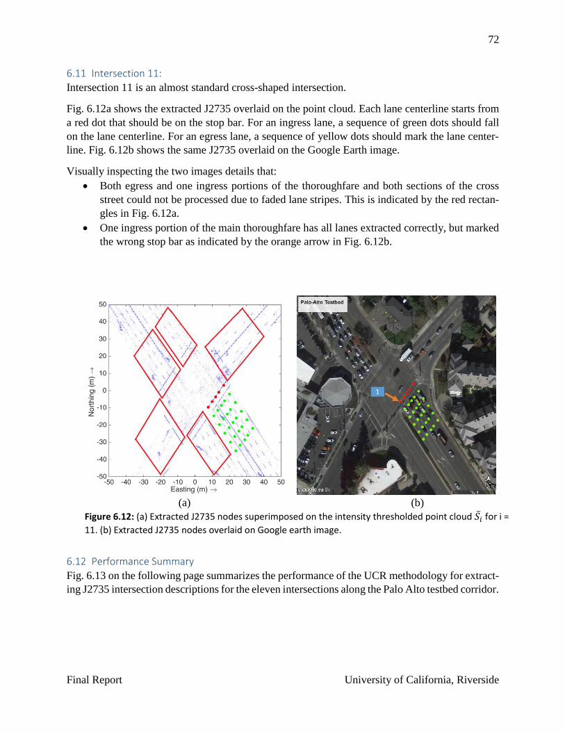
72
Final Report University of California, Riverside
6.11 Intersection 11:
Intersection 11 is an almost standard cross-shaped intersection.
Fig. 6.12a shows the extracted J2735 overlaid on the point cloud. Each lane centerline starts from
a red dot that should be on the stop bar. For an ingress lane, a sequence of green dots should fall
on the lane centerline. For an egress lane, a sequence of yellow dots should mark the lane center-
line. Fig. 6.12b shows the same J2735 overlaid on the Google Earth image.
Visually inspecting the two images details that:
Both egress and one ingress portions of the thoroughfare and both sections of the cross
street could not be processed due to faded lane stripes. This is indicated by the red rectan-
gles in Fig. 6.12a.
One ingress portion of the main thoroughfare has all lanes extracted correctly, but marked
the wrong stop bar as indicated by the orange arrow in Fig. 6.12b.
6.12 Performance Summary
Fig. 6.13 on the following page summarizes the performance of the UCR methodology for extract-
ing J2735 intersection descriptions for the eleven intersections along the Palo Alto testbed corridor.
(a) (b)
Figure 6.12: (a) Extracted J2735 nodes superimposed on the intensity thresholded point cloud 𝑆�̅� for i =
11. (b) Extracted J2735 nodes overlaid on Google earth image.

73
Final Report University of California, Riverside
Figure 6.13: Tabular summary of the J2735 intersection map extraction from MTLS data along the Palo Alto testbed corridor.
Surface
Detection
Lane Edge
Detection
Stop Bar
detection
Surface
Detection
Lane Edge
Detection
Stop Bar
Detection
1 Standard cross 8 of 8 100% 13 of 11 4 of 4 100% 8 of 8 4 of 4 2 • 2 bike lanes were detected in addition to traffic lanes
2 Non-Standard cross 8 of 8 100% 11 of 11 4 of 4 100% 8 of 8 4 of 4• 1 stop bar line has been detected and mapped at the
wrong line of the pedestrian cross walk
3 Non-Standard cross 8 of 8 100% 11 of 11 4 of 4 100% 8 of 8 4 of 4
• The direction of flow for one lane could not be
automatically determined because the mapping
vehicle did not drive in that ingress section.
4 Non-Standard cross 7 of 8 100% 9 of 20 2 of 4 100% 5 of 11 2 of 4
• 2 road segments (both ingress and egress) could not
be processed due to the non-standard road geometry
and faded lane striping.
5(a) Non-Standard T 6 of 6 100% 8 of 8 3 of 3 100% 7 of 7 2 of 3 2
• The direction of flow for one lane could not be
automatically determined because the mapping
vehicle did not drive in that ingress section.
• One stop bar has been detected manually because
stop bar marking was absent
5(b) Non-Standard T 6 of 6 100% 9 of 9 3 of 3 100% 7 of 7 2 of 3
• The direction of flow for one lane could not be
automatically determined.
• One stop bar has been detected manually because
stop bar marking was absent.
6 Non-Standard T 6 of 6 100% 10 of 10 3 of 3 100% 8 of 8 3 of 3• 1 misplaced stop bar is expected to be fixable in
future efforts.
7 Standard T 7 of 8 100% 9 of 9 3 of 3 100% 7 of 7 2 of 3 2 of 2
• The direction of flow for one lane could not be
automatically determined because the mapping
vehicle did not drive in that ingress section.
• 1 stop bar has been detected manually because stop
bar marking was absent.
• 1 misplaced stop bar is expected to be fixable in
future efforts.
8 Standard T 6 of 6 100% 9 of 9 3 of 3 100 7 of 7 2 of 3
• The programmer specified one stop bar due to the
absence of a painted stop bar on the road surface.
• The direction of flow for one lane could not be
automatically determined because the mapping
vehicle did not drive in that ingress section.
9 Non-Standard cross 4 of 8 100% 6 of 13 2 of 4 100% 4 of 8 2 of 4
• 2 road segments (both ingress and egress) could not
be processed due to the non-standard road geometry.
• 1 ingress lane could not be identified because there
was no trajectory information
10 Non-Standard cross 6 of 8 100% 9 of 11 3 of 4 100% 7 of 9 3 of 4• 2 road segments (both ingress and egress) could not
be processed due to the non-standard road geometry.
11 Standard cross 8 of 8 100% 4 of 14 1 of 4 100% 0 of 9 0 of 4• 2 road segments (both ingress and egress) could not
be processed due to the non-standard road geometry.
Intersection
Number
Intersection Type
(Standard cross,
Standard T, Non-
standard)
RemarksRoad Edge
Detection
Lanes
without
markings
Ingress Branch Egress Branch
Performance Analysis

74
Final Report University of California, Riverside
7. BEST PRACTICES FOR MTLS BASED AUTOMATED EXTRACTION OF
ROADWAY RELEVANT FEATURES This section summarizes several recommended practices based on the outcomes of the research
effort.
7.1 Equipment
LIDAR: As an active imaging sensor for roadway feature mapping, LIDAR should have
a field-of-view sufficient to simultaneously capture inner and outer roadway edges when
the vehicle is driven in the center lane.
High-resolution 360 degree camera: This sensor will enable photogrammetry to assist
visual interpretation.
Two-frequency carrier phase GNSS receiver: This enables high-precision (centimeter
accuracy) georectification (estimation of position and attitude) of the LIDAR and camera
data.
Inertial Measurement Unit (IMU): An IMU enables georectification to be implemented
at the high LIDAR (15-20 Hz) and camera rates (30 Hz), even though the GNSS makes
precise, independent position and attitude dependent measurements only at much lower
rates.
Differential GPS corrections: This is necessary to achieve the desired centimeter to dec-
imeter map position accuracy. One means of implementation is by a proximal (< 10 km)
base station. Another is by network computation of corrections. In either case, corrections
may be communicated by RF means in real-time or combined with GPS in post-pro-
cessing.
Power: Sufficient support power is required to run all equipment.
Data-storage: Sufficient to save the raw, time-stamped, sensor data over the time re-
quired to complete the data collection exercise.
7.2 Data collection procedure
The goal is to ensure a high-density of LIDAR reflections from roadway relevant features, to fa-
cilitate reliable automated extraction and mapping of those features.
Means to obtain a high-density of reflections:
The mapping vehicle should traverse each entry and exit point for each intersec-
tion a few times. These traverses should travel along different lanes. It is not neces-
sary to traverse each lane, but one traverse of the inner-most and outer-most lanes is
useful, due to the different perspectives that they provide. The tradeoff is that more
traverses gives a higher density of LIDAR reflections, different perspectives, and dif-
ferent obstructions; however, each traverse adds cost due to time, fuel, and data stor-
age.
Mapping vehicle should travel at reduced speeds (20-30mph), when appropriate.
The tradeoff is slower speeds provide gives a higher density of LIDAR reflections;
however, adds cost due to time and data storage requirements.

75
Final Report University of California, Riverside
Including multiple LIDAR’s, directly improves the density of reflections, per mile
driven.
Ensure that the LIDAR’s are mounted such that they illuminate the regions ex-
pected to contain the roadway features of interest.
Means to facilitate automatic extraction of features:
In post-processing, the GNSS and IMU data will be used to estimate the platform tra-
jectory and to geo-rectify the LIDAR and camera data. Both the geo-rectified data
and the platform trajectory should be saved for the feature extraction pro-
cessing. The platform trajectory provides useful data, such as the number of intersec-
tion entry and exit points and direction of travel along each.
For roads without a meridian, to aid the automatic extraction of the divider between
ingress and egress lanes, the mapping vehicle should be driven along those lanes
nearest to this divider. This is recommended so that the direction-of-travel metadata
for each lane can be extracted.
Means to avoid occlusion of roadway features:
Fore and aft rolling closure and/or traffic break minimizes artifacts from vehicle in-
trusions.
Performing multiple traverses provides multiple opportunities to receive reflections
from each roadway feature. The traverses occurring at different time improves the
chances that the occluding object is no longer occluding the same features.
Means to confirm accuracy:
Occasional control points (known locations) consisting of highly reflective material
allows both instrument calibration and confirmation of the accuracy of mapped fea-
tures.
7.3 Data post processing
After determining the platform trajectory and collecting the georectified LIDAR point cloud and
camera photolog, the key recommendations for data post processing are as follows:
Retain the raw sensor data as long as possible.
Retain the point cloud data for the entire roadway region of interest.
Utilize control points to assist with calibration, validation, and merging of data sets.
For georectification and feature mapping use a consistent Earth Center Earth Fixed
(ECEF) reference frame in addition to other formats (state plane; latitude, longitude, ele-
vation)
In the mapping of intersections, the following have also proved useful:
Define a reduced point cloud for each intersection, for example all points within a radius
R for the defined origin of the intersection.
Within this region, process the sensor platform trajectory to determine the number of ap-
proaches and exits to the intersection.

76
Final Report University of California, Riverside
From the intersection point cloud, extract a subset that represents one approach or exit.
Filter and remove data from interfering objects (e.g., vehicles, trees, people). This can be
accomplished for example by extracting from the point cloud only those points that form
a smooth two-dimensional surface, discarding any points too far from that surface.
Perform feature extraction as necessary for the application of interest.
Use the sensor platform trajectory to specify directions of travel metadata.
Store the extracted lane markings, road edges, and other features of interest with preci-
sion (perhaps 10 times) greater than the desired accuracy of the map.

77
Final Report University of California, Riverside
8. CONCLUSIONS Connected Vehicle applications require roadway feature digital maps stored and communicated
using uniform methods for representation and reference. These maps must conform to well under-
stood accuracy specifications to ensure the safety of life and infrastructure. Due to the scope of the
mapping requirements, when considered at the national and global scales, automated and data
driven mapping approaches must be considered.
Numerous methods exist to acquire and record data indicative of geospatial objects and terrain.
Based on our analysis, the preferred existing acquisition methods for roadway mapping utilize
GPS/IMU integrated LIDAR sensing to generate a three dimensional georectified point cloud data
set. At present, the state of the art approaches to feature extraction are human intensive. When data
acquisition is conducted with multiple integrated sensors at a high frequency and national (or
global) scale, the resulting dataset is sufficiently large that automated and application specific data
processing become necessary for economic feasibility. This project report has presented an auto-
mated feature extraction approach and demonstrated its use on eleven intersections. The resulting
processed dataset presented herein provides a meaningful representation of roadway features of
interest for intersections, while excluding irrelevant data.
The roadway feature extraction process included the following primary steps:
Preprocessing to extract the georectified point cloud and associated trajectory portions of
interest for given intersections;
Identification and extraction of the road surface point cloud, road edge curves, and median
edge curves;
Conversion of the intersection road surface point cloud to an image to enable feature ex-
traction by image processing methods;
Image-based roadway feature extraction; and
Translation to a J2735 feature map for intersections of interest.
This methodology for feature extraction and map representation has been presented with a detailed
explanation of data processing and integration. This detailed approach allows for future feature
extraction of relevant roadway features in connected vehicle environments.
Mapping needs relevant to the USDOT Connected Vehicle Pilot Deployment Program are dis-
cussed in Appendix C.
The analysis of the algorithm performance shows that it works very well for “standard” intersec-
tions. However, additional work is required to achieve functionality for non-standard intersections.
Also, on the continuum between manual and fully automated, the algorithms described in Chapter
5 are somewhere in the middle, and are considered to be human-assisted. When the algorithm
detects an anomalous situation, it stops to alert the human before moving further forward. This is
considered good practice as the generated maps have implications for human safety. The authors
caution against learning or deep learning approaches as they cannot discriminate those portions of
the map that are certain and those that are not.

78
Final Report University of California, Riverside
9. FUTURE WORK The feature extraction methodology and its evaluation on eleven intersections demonstrate the
complexity of representing relevant roadway features in a standard usable format within a con-
nected vehicle environment. The algorithm worked well in spite of these complexities, making a
significant advance from manual feature extraction toward automated data processing for roadway
relevant feature extraction. Following are a few avenues fruitful for future efforts:
Georectification: The accuracy of roadway feature maps rests upon the georectification
process. That step relies on accurate and reliability knowledge of the sensor platform tra-
jectory during data acquisition. Both accuracy and reliability are challenging in dense ur-
ban environments where GNSS signals are not reliable. Multisensor approaches fusing
GNSS, LIDAR, Camera and IMU data should be investigated.
Feature Extraction and Mapping: Several directions are available for future work:
o This project focused on lane edges and stop bars. The method worked well in a
semi-automated fashion for standard intersections. Advancing toward more fully
automated processes enhances the rate and decreases the cost of roadway mapping.
o Methods should be developed to accommodate more complex, non-standard inter-
sections.
o As CV applications develop, additional features will become of interest. Additional
feature extraction algorithms will be required, across a wide range of roadways and
features.
o This effort has worked with georectified LIDAR point clouds. Also including
georectified photologs in the automated processing could yield enhanced reliability
and performance.
Research should be done in conjunction with government agencies, academic groups, and
commercial entities for testbed applications and demonstration projects that require road-
way relevant maps and allow the opportunity for advancements within the automated map-
ping field.
Crowd-sourced data: This area is in its infancy and could yield more efficient approaches
for detecting the need for map database updating; collection of map metadata such as in-
tersection lane connectivity; and real-time detection of road hazards.
Integration of Crowd-sourced and MTLS: Crowd-sourced and MTLS data have very
different characteristics in accuracy, security, reliability, and timeliness. Studies of how to
securely and effectively combine this information is critical.
CV Application Mapping Requirements: As CV pilot deployments progress the
achieved mapping and vehicle positioning accuracy should be noted and studied relative
to the performance and capabilities that could have been achieved with greater accuracy.
Development and Demonstration: The approach presented herein was limited in scope
to a small set of intersections (11) and specific features. Broadening this to a larger set of
intersections across the country is critical for characterizing existing capabilities and dis-
covering their strengths and weaknesses prior to large scale deployment.

79
Final Report University of California, Riverside
Evolution of geospatial data acquisition will yield increasingly accurate and reliable topology data
for the roadway environment. The necessity to identify and automatically extract relevant roadway
features will become significantly more valuable. The methodology presented herein focused on
roadway attributes associated with intersection relevant road surface features. It should be viewed
as a glimpse of what is possible in the future as the technology develops. Present and future sensing
and computing resources are not the limiting factors. This field is in its infancy. Feature extraction
algorithms, mapping standards, commercial approaches, and potential connected vehicle applica-
tions are still in their formative and demonstration phases.

80
Final Report University of California, Riverside
BIBLIOGRAPHY [1] A. Vu, J. A. Farrell, M. Barth, “Centimeter-Accuracy Smoothed Vehicle Trajectory Esti-
mation,” IEEE Intelligent Transportation Magazine, pp. 121-135, Winter 2013.
[2] K. Yen, B. Ravani, and T. A. Lasky, “Mobile Terrestrial Laser Scanning Workflow devel-opment, Technical Support and Evaluation,” UCD-ARR-14-06-14-01, June 14, 2014.
[3] IGS, International GNSS Service, RINEX: The Receiver Independent Exchange Format, Version 3.02, ftp://igs.org/pub/data/format/rinex302.pdf, April 3, 2013.
[4] ASPRS Board, LAS file format specification, http://www.asprs.org/a/society/commit-tees/standards/asprs_las_format_v12.pdf, Sept. 2, 2008.
[5] NDS: Navigation Data Standard Website, http://www.nds-association.org/, accessed July 30, 2015.
[6] SAE International, J2739 Standard, “Dedicated Short Range Communication (DSRC) Message Set Dictionary,” http://standards.sae.org/j2735_200911/, November 19, 2009.
[7] A. Vu, J. A. Farrell, “Feature Mapping and State Estimation for Highly Automated Vehi-cles,” Journal of Control and Decision, 2:1, 1-25, 2015.
[8] C. E. Cohen, B. D. McNally, B. W. Parkinson, “Flight Tests of Attitude Determination using GPS Compared against an Inertial Navigation Unit,” ION National Technical Meet-ing, Jan. 1993.
[9] B. Triggs, P. Mclauchlan, R. Hartley, A. Fitzgibbon, “Bundle Adjustment—A Modern
Synthesis,” HAL, Dec. 20, 2010.
[10] R. M. Eustice, H. Singh, J. J. Leonard, “Exact Sparse Delayed-State Filters for View-Based SLAM,” IEEE T. Robotics, 22:6, pp. 1100-1114, 2006.
[11] F. Dellaert, M. Kaess, “Square Root SAM: Simultaneous Localization and Mapping via Square Root Information Smoothing,” Int. J. of Robotics Research, pp. 1181-1203, Dec. 2006.
[12] S. Ibrahim and D. Lichti, 2012. Curb-Based Street Floor Extraction from Mobile Terres-trial LIDAR Point Cloud, ISPRS - International Archives of the Photogrammetry, Remote Sensing and Spatial Information Sciences, Volume XXXIX-B5, pp.193-198, 2012.
[13] B. Yang, L. Fang, Q. Li, J. Li, "Automated Extraction of Road Markings from Mobile LIDAR Point Clouds," Photogrammetric Engineering & Remote Sensing, 8: 4, pp. 331-338, 2012.
[14] B. Yang, L. Fang, J. Li, “Semi-automated extraction and delineation of 3D roads of street scene from mobile laser scanning point clouds,” ISPRS J. of Photogrammetry and Re-mote Sensing, 79, 80-93, 2013.
[15] B. Yang, Z. Wei, Q. Li, J. Li, “Automated extraction of street-scene objects from mobile LIDAR point clouds,” International J. of Remote Sensing, 33(18): 5839-5861, 2012.
[16] P. Kumar, Conor P. McElhinney, P. Lewis, T. McCarthy, "Automated road markings ex-traction from mobile laser scanning data," International J. of Applied Earth Observation and Geoinformation, 32, Pages 125–137, Oct. 2014
[17] H. Guan, J. Li, Y. Yu, M. Chapman, C. Wang, "Automated Road Information Extraction From Mobile Laser Scanning Data," IEEE T. Intelligent Transportation Systems, 16:1, pp 194-205, 2014
81
Final Report University of California, Riverside
[18] H. Guan, J. Li, Y. Yu, Z. Ji, C. Wang, “Using mobile LIDAR data for rapidly updating road markings,” IEEE Transactions on Intelligent Transportation Systems, DOI: 10.1109/ TITS.2015.2409192, 2015.
[19] H. Guan, J. Li, Y. Yu, C. Wang, M. Chapman, B. Yang, "Using mobile laser scanning data for automated extraction of road markings," ISPRS J. of Photogrammetry and Remote Sensing, 87, pp. 93–107, January 2014.
[20] Y. Yu, J. Li, H. Guan, F. Jia, C. Wang, “Learning hierarchical features for automated ex-traction of road markings from 3-D mobile LIDAR point clouds,” IEEE J. of Selected Top-ics in Applied Earth Observations and Remote Sensing, 8(2): 709-726, 2015
[21] S. Kieval, "Aerial, Mobile and Terrestrial LIDAR." 2015 ESRI Petroleum GIS Conference Proceedings, Apr. 2015.
[22] D. Berber, J. Mills, S. Smith-Voysey, “Geometric validation of a ground-based mobile laser scanning system,” Photogrammetry and Remote Sensing, 63, pp. 128-141, 2008.
[23] D. Forsyth and J. Ponce, Computer Vision: A Modern Approach (second edition), Pearson Publishing, New York, ISBN-13: 978-0136085928].
[24] ED-Map, “Enhanced Digital Mapping Project, final report, November 19, 2004.
[25] MTA, Mapping Technology Assessment for Connected Vehicle Highway Network Appli-cations, Booz, Allen, Hamilton, September 2012.
[26] B. Spear, A. Vandervalk, D. Snyder, “Roadway Geometry and Inventory Trade Study for IntelliDrive Applications,” FHWA-HRT-10-073, November 2010.
[27] J. A. Farrell, M. Todd, and M. Barth, “Best Practices for Surveying and Mapping Road-
ways and Intersections for Connected Vehicle Applications,” Task 1 Report: Mapping
Methodology Assessment, University of California Riverside, August 4, 2015.
[28] DSRC Implementation Guide: A guide to users of SAE J2735 message sets over DSRC, SAE International, Feb. 16, 2010.
[29] Enhanced Digital Mapping Project, Final Report, CAMP, November 19, 2004.
[30] Mapping Technology Assessment for Connected Vehicle Highway Network Applications, Final Report, Booz, Allen, Hamilton, September 2012.
[31] D. Betaille, R. Toledo-Moreo, Creating Enhanced Maps for Lane-Level Vehicle Naviga-tion. IEEE Transactions on Intelligent Transportation Systems, 11(4), 786-798, 2010.
[32] J. Liu, B. Cai, Y. Wang, J. Wang, “Generating Enhanced Intersection Maps for Lane Level Vehicle Positioning based Applications,” Procedia: Social and Behavioral Sciences, 96, pp. 2395-2403, 2013.
[33] N. Mohammed, A. Ghazi and H. E. Mustafa, “Positional Accuracy Testing of Google
Earth,” International Journal of Multidisciplinary Sciences And Engineering, Vol. 4, No.
6, July 2013.
[34] C. Paredes-Hernandez, W. Salinas-Castillo, F. Guevara-Cortina and X. Martinez-Becerra,
“Horizontal Positional Accuracy of Google Earth’s Imagery Over Rural Areas: A Study
Case in Tamaulipas, Mexico,” BCG - Boletim de Ciências Geodésicas - On-Line version,
ISSN 1982-2170.

82
Final Report University of California, Riverside
[35] A. Farah and D. Algarni, “Positional Accuracy Assessment of Google Earth in Riyadh,”
Artificial Satellites, Vol. 49, No. 2 – 2014.
[36] California State Transportation Agency, “California Manual on Uniform Traffic Control
Devices,” p. 653, 2014, URL: http://www.dot.ca.gov/hq/traffops/engineering/mutcd/pdf/ca-
mutcd2014/CAMUTCD2014.pdf
[37] University of California-Riverside, “The role of crowd-sourced trajectory data in road-
way feature mapping”, pending technical report.

83
Final Report University of California, Riverside
APPENDIX A: ACRONYM DEFINITIONS ALS – Aerial Laser Scanner
CV – Connected Vehicles
DOT – Department of Transportation
GNSS – Global Navigation Satellite Systems
IMU – Inertial Measurement Unit
LAS – American Society for Photogrammetry and Remote Sensing laser file format
LIDAR – Light Detection and Ranging
MIRE – Model Inventory of Roadway Elements
MMITSS – Multi-Modal Intelligent Traffic Signal System
MMSTS – Manufacturing Major Subsystem Technical Specification
MTLS – Mobile Terrestrial Laser Scanner
NCHRP – National Cooperative Highway Research Program
PPM – Points per square meter
RINEX – Receiver Independent Exchange Format
STLS – Stationary Terrestrial Laser Scanner
UAV – Autonomous Aerial Vehicle

84
Final Report University of California, Riverside
APPENDIX B: CONTACTS This report was written in part using notes from many interviews with the people noted below. We
greatly appreciate their enthusiasm in discussing the related topics. The report has not yet been
distributed for comment. All statements and any errors are the responsibility of the authors.
People Interviewed:
Name Organization Phone Email Date
James Appleton Caltrans 916-227-7656 [email protected] 4-9-‘15
Terry Bills ESRI 909-793-2853 [email protected]
Stan Burns Utah DOT 801-633-6221 [email protected] 3-24-‘15
John Cassidy TomTom 603-290-2476 [email protected] 6-11-‘15
John Caya Mandli 608.835.3500 [email protected] 4-10-‘15
Dan Dailey FHWA 202-493-3395 [email protected]
Walt Fehr USDOT 202-366-0278 [email protected]
Robert Ferlis FHWA 202-493-3268 [email protected]
Matt Friedman Caltrans 916-654-4823 [email protected] 3-24-‘15
Keith Hangland HERE 303-974-8111 [email protected] 4-21-‘15
Larry Head Arizona University 520-621-2264 [email protected] 5-18-‘15
David Kelley SAE 2735 Committee 626-513-7715 [email protected] 4-14-‘15
Ty Lasky AHMCT, UC-Davis 530-752-6366 [email protected] 6-24-‘15
Elmain Mair Bosch
Hesham Rakha Virginia Tech 540-231-1505 [email protected] 5-8-‘15
Ron Singh Oregon DOT 503-986-3033 [email protected] 4-14-‘15
Mark Turner Caltrans 916-227-7669 [email protected] 4-9-‘15
Kin Yen AHMCT, UC Davis 530-754-7401 [email protected] 6-24-‘15
Wei-Bin Zhang PATH, UC Berkeley 510 665-3515 [email protected] 5-18-‘15
Kun Zhou PATH, UC Berkeley 510 665-3666 [email protected] 5-18-‘15

85
Final Report University of California, Riverside
APPENDIX C: USDOT CONNECTED VEHICLE PILOT DEPLOYMENT PRO-
GRAM: MAPPING NEEDS As part of the Connected Vehicle Pilot Deployment (CVPD) Program, in late 2015, the USDOT
selected three U.S. sites to deploy large scale connected vehicle applications. In this appendix, we
briefly describe these different CVPD locations, their applications, and potential mapping needs.
This is based on information available as of May 2016. It should be noted that these CVPD sites
are currently defining their detailed concept of operations for various CV applications and are not
yet available publically.
Interstate-80 (I-80) Wyoming
I-80 is a major commercial and goods movement corridor with 30% to 70% of the road traffic
consisting of heavy-duty trucks. The length of I-80 extends greater than 400 miles with large por-
tions consisting of mountain passes at elevation greater than 7000 ft.
Due in part to challenging weather conditions, I-80 has an elevated frequency of collisions and
vehicular accidents. The weather conditions considered to increase travel risks include poor visi-
bility due to heavy snow or fog, icy roads, and high winds. Winds exceeding 65 mph impact high
profile vehicles especially when empty or lightly loaded. An additional challenge is providing
route closure and parking information to the drivers during closure events lasting many hours.
Much of I-80 is located in rural areas with towns located 45 to 150 miles apart with little or no
parking facilities in between. Fig 13.1 shows the map of this Wyoming CVPD site.
Figure 13.1: Map of Wyoming CVPD site.
The Connected Vehicle applications proposed for I-80 address the inherent safety issues described
above. This includes a variety of road weather applications. Roadway weather information can be
linked with enabled connected vehicles and will alert drivers to hazardous weather conditions,
roadway closures, and contingency planning. Other Connected Vehicle applications will allow
equipped vehicles to monitor roadway and vehicle conditions in close proximity.
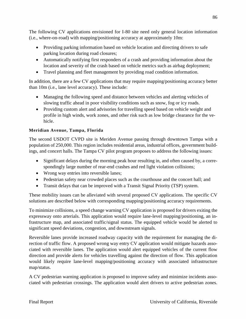
86
Final Report University of California, Riverside
The following CV applications envisioned for I-80 site need only general location information
(i.e., where-on-road) with mapping/positioning accuracy at approximately 10m:
Providing parking information based on vehicle location and directing drivers to safe
parking location during road closures;
Automatically notifying first responders of a crash and providing information about the
location and severity of the crash based on vehicle metrics such as airbag deployment;
Travel planning and fleet management by providing road condition information.
In addition, there are a few CV applications that may require mapping/positioning accuracy better
than 10m (i.e., lane level accuracy). These include:
Managing the following speed and distance between vehicles and alerting vehicles of
slowing traffic ahead in poor visibility conditions such as snow, fog or icy roads.
Providing custom alert and advisories for travelling speed based on vehicle weight and
profile in high winds, work zones, and other risk such as low bridge clearance for the ve-
hicle.
Meridian Avenue, Tampa, Florida
The second USDOT CVPD site is Meriden Avenue passing through downtown Tampa with a
population of 250,000. This region includes residential areas, industrial offices, government build-
ings, and concert halls. The Tampa CV pilot program proposes to address the following issues:
Significant delays during the morning peak hour resulting in, and often caused by, a corre-
spondingly large number of rear-end crashes and red light violation collisions;
Wrong way entries into reversible lanes;
Pedestrian safety near crowded places such as the courthouse and the concert hall; and
Transit delays that can be improved with a Transit Signal Priority (TSP) system.
These mobility issues can be alleviated with several proposed CV applications. The specific CV
solutions are described below with corresponding mapping/positioning accuracy requirements.
To minimize collisions, a speed change warning CV application is proposed for drivers exiting the
expressway onto arterials. This application would require lane-level mapping/positioning, an in-
frastructure map, and associated traffic/signal status. The equipped vehicle would be alerted to
significant speed deviations, congestion, and downstream signals.
Reversible lanes provide increased roadway capacity with the requirement for managing the di-
rection of traffic flow. A proposed wrong way entry CV application would mitigate hazards asso-
ciated with reversible lanes. The application would alert equipped vehicles of the current flow
direction and provide alerts for vehicles travelling against the direction of flow. This application
would likely require lane-level mapping/positioning accuracy with associated infrastructure
map/status.
A CV pedestrian warning application is proposed to improve safety and minimize incidents asso-
ciated with pedestrian crossings. The application would alert drivers to active pedestrian zones.
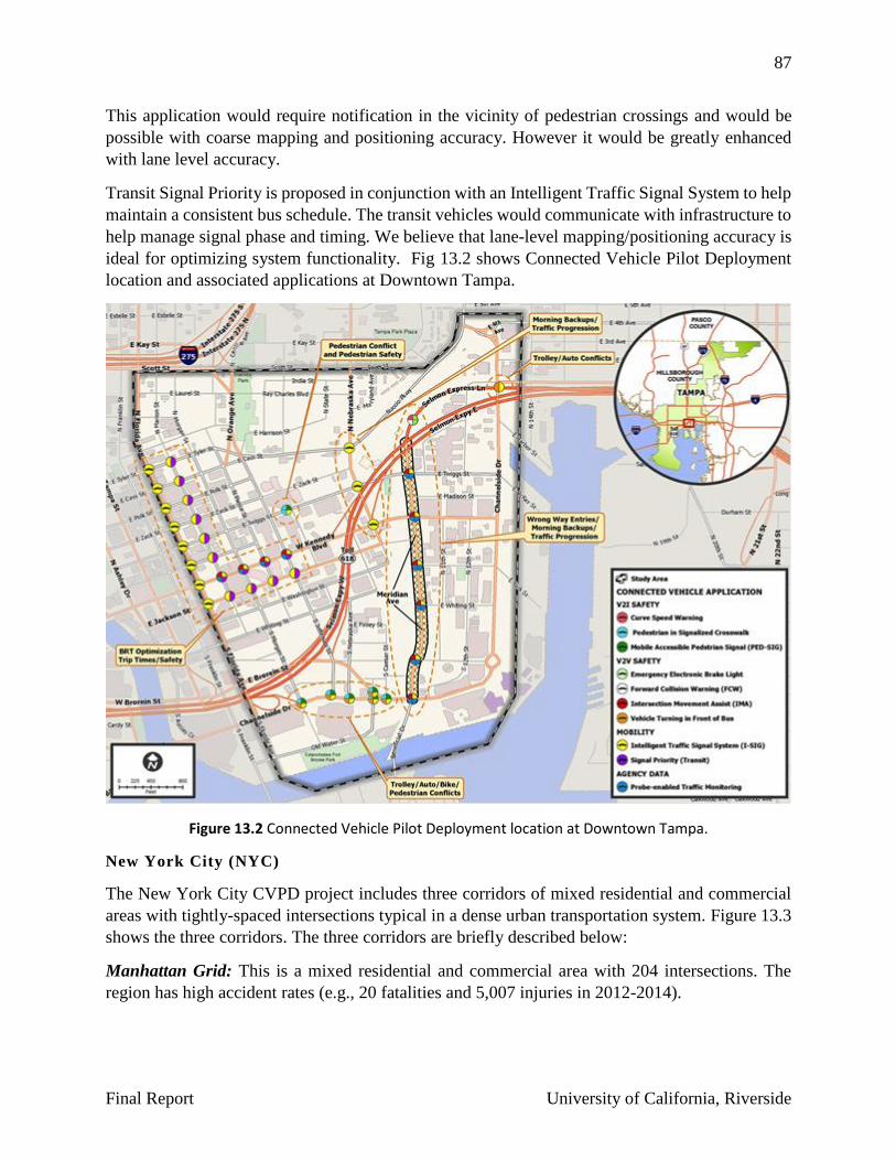
87
Final Report University of California, Riverside
This application would require notification in the vicinity of pedestrian crossings and would be
possible with coarse mapping and positioning accuracy. However it would be greatly enhanced
with lane level accuracy.
Transit Signal Priority is proposed in conjunction with an Intelligent Traffic Signal System to help
maintain a consistent bus schedule. The transit vehicles would communicate with infrastructure to
help manage signal phase and timing. We believe that lane-level mapping/positioning accuracy is
ideal for optimizing system functionality. Fig 13.2 shows Connected Vehicle Pilot Deployment
location and associated applications at Downtown Tampa.
Figure 13.2 Connected Vehicle Pilot Deployment location at Downtown Tampa.
New York City (NYC)
The New York City CVPD project includes three corridors of mixed residential and commercial
areas with tightly-spaced intersections typical in a dense urban transportation system. Figure 13.3
shows the three corridors. The three corridors are briefly described below:
Manhattan Grid: This is a mixed residential and commercial area with 204 intersections. The
region has high accident rates (e.g., 20 fatalities and 5,007 injuries in 2012-2014).

88
Final Report University of California, Riverside
Manhattan FDR Dr.: This is a limited access highway which excludes trucks and buses. It has
short radius curves and over-height restrictions.
Brooklyn Flatbush Ave.: This roadway has an average speed of 15 mph along 35 intersections. It
is a high accident rate arterial with 1,128 injuries and 8 fatalities in 2012-2014.
A B c Figure 13.3 NYC deployment sites. a) Manhattan Grid. b) Manhattan FDR. c) Flatbush Ave.
The primary objective of the NYC CV Pilot deployment site is to improve the safety of travelers
and pedestrians in New York City through connected vehicle technologies. The mobility and safety
issues that are to be addressed are as follows:
Discourage spot speeding;
Reduce accidents at high incident intersections;
Improve pedestrian safety and reduce bus related crashes on heavily traveled bus routes;
Improve safety of for disabled pedestrians (V2P);
Improve truck safety;
Address bridge low clearance issues;
Enforce truck route restrictions;
Improve work zone safety;
Balance mobility in heavily congested areas; and
Reduce crashes, injuries and delays.
The targeted improvements in the highly congested region will require a high accuracy maps with
coordinated status between vehicles and infrastructure. Lane-level mapping/positioning will be
required for almost all of the CV applications due to vehicular density and pedestrian interaction.
Generalized driver notification of roadway status can be achieved with low mapping/positional
accuracies, however applications targeted at specific vehicles and driver behavior will require in-
creased mapping/positional accuracy with corresponding infrastructure information. Another sig-
nificant concern is that many of the NYC CV applications will be carried out in areas where GPS
signals are blocked or suffer from a high degree of multi-path error. Both mapping and positioning
methods will need to deal with these potential problems.

89
Final Report University of California, Riverside
This brief review of CVPD programs provides initial insight into the mapping, vehicular, and po-
sitional requirements for the proposed implementations. Each application discussed has the poten-
tial to achieve higher levels of performance with improvements to positional accuracies, infra-
structure maps, and related data. This review serves as a general guide with the expectation that
any single CV application will undergo a thorough analysis for specific roadway conditions and
system requirements.