establishing tools to optimize surface traps for wiring up...
TRANSCRIPT

Establishing tools to optimizesurface traps for wiring up
trapped ions.
Dissertation
zur Erlangung des Doktorgrades an der
Fakultat fur Mathematik, Informatik und Physikder Leopold-Franzens-Universitat Innsbruck
vorgelegt von
Sankaranarayanan Selvarajan
durchgefuhrt am Institut fur Experimentalphysik
unter der Leitung vonDr. Hartmut Haffner
Innsbruck, 2017


Abstract
The ability to store, control, split and transport large ion strings and theease of fabrication, makes surface traps a promising technology for scaling upion trap quantum computation. However, despite the advantages of this traparchitecture, some important issues remain unsolved. On the one hand, wellestablished micromotion compensation methods used in linear Paul trap cannotbe easily extended to surface trap setup. On the other hand, the heating ratesobserved in surface trap are orders higher than the predicted value and thetheoretical model proposed to explain this still needs vindication. To harness thefull potential of the surface traps these problems needs to be addressed. In thiswork we present the experimental tools we developed to address some of theseproblems.
Conventional methods used to detect micromotion in linear Paul traps useDoppler shift induced by the ion motion to detect micromotion. This requiresthe laser beam to have a projection on all three directions of the ion motion.In a planar trap setup, the distance of the trapped ions from the surface of thetrap is very small compared to the width of the trap. This limits the laser beamalignment to be parallel to the surface of the trap. This implies the projectionof the laser beam on the motional mode of the ion perpendicular to the trapsurface is almost zero. This makes the extension of these micromotion detectionmethods to surface traps difficult. In this thesis we present a novel micromotioncompensation method well suited for surface traps. This method is simple anddoes not required ultra stable, low line-width lasers.
Another important problem that has to be solved before the surface trapscan be used for quantum computation experiments is the excess heating rates.The heating rates observed in the surface traps are more than 3 orders higherthan expected from Johnson noise. The different models proposed to explainthis observed heating rate are not verified yet. In this thesis we present themeasurements of heating rates carried out at various positions along the axis ofthe trap. This knowledge can lead to a better understanding of the cause of theelectric field fluctuations in the ion trap setup.
Lastly, we present a theoretical analysis of a new method to scale-up ion trapsby coupling ions using a macroscopic metallic wire. We also present the firstexperiments performed to assess the influence of the wire on the ion.
i


Zusammenfassung
Oberflachenfallen eignen sich hervoragend um selbst große Ionenkristallezu speichern, zu teilen und zu transportieren. Daruber hinaus lassen sichmit ihnen auch selbst komplexe Elektrodenkonfiguration leicht herzustellen.Diese Eigenschaften machen Oberflachenfallen als skalierbare Architektur furQuanteninformationsverarbeitung sehr interessant. Trotz dieser Vorteile, bleibenviele wichtige Fragen offen. Zum Einen, sind die in herkommlichen Paulfallenbenutzten Techniken zur Mikrobewegungskompensation nicht ohne weiteresauf Oberflachenfallen ubertragbar. Zum Anderen sind die gemessenen Heizratender Ionenbewegung in Oberflachenfallen um ein Vielfaches hoher als erwartetund Modelle, die solche erhohten Heizraten vorhersagen konnen, sind schwerzu uberprufen. Um das volle Potenzial von Oberflachenfallen auszuschopfen,mussen diese Fragen angegangen werden. Diese Arbeit etabliert Werkzeuge,die helfen konnen, diese Probleme zu losen.
Herkommliche Methoden, um Mikrobewegung in linearen Paulfallen zudetektieren, benutzen den Dopplereffekt der aus der Bewegung der Ionen resultiert.Dies bedeutet, dass Laserlicht mit einer Projektion auf all Raumrichtungenverfugbar sein muss. Allerdings sind die Ionen in einer Oberflachenfalle imVerhaltnis zur Ausdehnung der Oberflachenfalle sehr nahe an der Oberflachegespeichert. Daher ist es schwer, eine signifikante Projektion des Laserlichtssenkrecht zur Oberflache zu erreichen mit der Folge, dass die meisten Technikenzur Mikrobewegungskompensation nicht auf Oberflachenfallen ubertragbar sind.In dieser Arbeit prasentieren wir eine neuartige Methode zur Mikrobewegungs-kompensation, die kompatibel mit Oberflachenfallen ist. Unsere Technik istunkompliziert und benotigt keine stabilen schmalbandige Laser.
Das andere wichtige Problem, bevor Oberflachenfallen gewinnbringend zurQuanteninformationsverarbeitung eingesetzt werden konnen, sind Heizraten,die ca. drei Großenordnungen hoher sind als man es von Johnson-Rauschen derElektronik erwartet. Die verschiedenen theoretischen Modelle, die dies erklarensollen, konnten bis jetzt noch nicht experimentell uberpruft werden. In dieserArbeit prasentieren wir Heizratenmessungen fur Ionen, die uber verschiedenenStellen der Fall gespeichert wurden. Unsere Resultate tragen zu einem besserenVerstandnis der moglichen Mechanismen bei, die elektrisches Feldrauschen unddamit die erhohten Heizraten erzeugen.
Als letztes diskutieren wir eine theoretische Analyse einer neuartigen Methodebei der Ionen uber metallische Drahte gekoppelt werden, um die Ionenfallen-technologie zu skalieren. In diesem Zusammenhang prasentieren wir ersteexperimentelle Resultate, die den Einfluss einen Drahtes auf die Ionebewegungcharakterisieren.


Contents
Contents i
List of Figures iii
List of Tables v
1 Introduction 11.1 Thesis outline . . . . . . . . . . . . . . . . . . . . . . . . . . . . . . 3
2 Theory 52.1 Trapping and controlling ions . . . . . . . . . . . . . . . . . . . . . 5
2.1.1 Linear Paul traps . . . . . . . . . . . . . . . . . . . . . . . . 52.1.2 Planar surface traps . . . . . . . . . . . . . . . . . . . . . . 82.1.3 Efficient control of DC voltages . . . . . . . . . . . . . . . . 9
2.2 Quantum mechanics of trapped ions coupled to light fields . . . . 142.2.1 Motional Hamiltonian . . . . . . . . . . . . . . . . . . . . . 142.2.2 Two-level system . . . . . . . . . . . . . . . . . . . . . . . . 152.2.3 Laser-Ion interaction . . . . . . . . . . . . . . . . . . . . . . 16
2.3 Laser-cooling of trapped ions . . . . . . . . . . . . . . . . . . . . . 182.3.1 level scheme of 40Ca+ . . . . . . . . . . . . . . . . . . . . . 182.3.2 Doppler cooling . . . . . . . . . . . . . . . . . . . . . . . . . 192.3.3 Sideband cooling . . . . . . . . . . . . . . . . . . . . . . . . 20
2.4 Detection of the motional state . . . . . . . . . . . . . . . . . . . . 222.4.1 Motional sideband methods . . . . . . . . . . . . . . . . . . 222.4.2 Doppler recooling method . . . . . . . . . . . . . . . . . . . 24
2.5 Wiring up trapped ions . . . . . . . . . . . . . . . . . . . . . . . . . 242.5.1 Coupling mechanism . . . . . . . . . . . . . . . . . . . . . . 252.5.2 Sources of decoherence . . . . . . . . . . . . . . . . . . . . 29
3 Experimental setup 313.1 General Infrastructure . . . . . . . . . . . . . . . . . . . . . . . . . 31
i

ii CONTENTS
3.1.1 Surface traps . . . . . . . . . . . . . . . . . . . . . . . . . . 313.1.2 Optics and laser system . . . . . . . . . . . . . . . . . . . . 353.1.3 Vacuum chamber assembly . . . . . . . . . . . . . . . . . . 393.1.4 Coupling wire assembly . . . . . . . . . . . . . . . . . . . . 413.1.5 Magnetic field coils . . . . . . . . . . . . . . . . . . . . . . . 43
3.2 Voltage source . . . . . . . . . . . . . . . . . . . . . . . . . . . . . . 433.2.1 RF Voltage . . . . . . . . . . . . . . . . . . . . . . . . . . . . 443.2.2 DC Voltage . . . . . . . . . . . . . . . . . . . . . . . . . . . 45
3.3 Experimental control . . . . . . . . . . . . . . . . . . . . . . . . . . 45
4 Stray electric field sensing and compensation 494.1 Micromotion in ion traps . . . . . . . . . . . . . . . . . . . . . . . . 49
4.1.1 Principle of compensation . . . . . . . . . . . . . . . . . . 504.1.2 Implementation . . . . . . . . . . . . . . . . . . . . . . . . . 51
4.2 Electric field sensing . . . . . . . . . . . . . . . . . . . . . . . . . . 554.3 Possible sources of the stray electric field . . . . . . . . . . . . . . 59
4.3.1 Abrupt change in the stray fields . . . . . . . . . . . . . . . 594.3.2 Photoionization . . . . . . . . . . . . . . . . . . . . . . . . 614.3.3 Electrical field emission . . . . . . . . . . . . . . . . . . . . 63
4.4 Clean trap surfaces for reduced charging . . . . . . . . . . . . . . 64
5 Heating in ion traps 675.1 Heating rate measurement techniques . . . . . . . . . . . . . . . . 67
5.1.1 Sideband comparison method . . . . . . . . . . . . . . . . 695.1.2 Rabi flopping . . . . . . . . . . . . . . . . . . . . . . . . . . 695.1.3 Doppler recooling method . . . . . . . . . . . . . . . . . . . 71
5.2 Heating rate along the axis of the trap . . . . . . . . . . . . . . . . 76
6 Towards coupling ions using a macroscopic wire 776.1 Trapping simultaneously in two independent wells . . . . . . . . 776.2 Wire position measurement . . . . . . . . . . . . . . . . . . . . . . 796.3 Characterization of potentials . . . . . . . . . . . . . . . . . . . . . 806.4 Characterization of secular frequencies . . . . . . . . . . . . . . . . 856.5 Characterization of Heating rates . . . . . . . . . . . . . . . . . . . 86
7 Summary 897.1 Outlook . . . . . . . . . . . . . . . . . . . . . . . . . . . . . . . . . . 90
Bibliography 91
A Quantum state transfer between coupled ions 99

List of Figures
2.1 Paul trap structure and resultant quadrupole . . . . . . . . . . . . . . 62.2 Dynamics of Paul trap . . . . . . . . . . . . . . . . . . . . . . . . . . . 62.3 Linear trap to surface trap transformation . . . . . . . . . . . . . . . . 82.4 Multipole expansion . . . . . . . . . . . . . . . . . . . . . . . . . . . . 132.5 Coupled energy levels and motional sidebands . . . . . . . . . . . . . 172.6 The level structure of a 40Ca+ ion . . . . . . . . . . . . . . . . . . . . . 182.7 Schematic of sideband cooling . . . . . . . . . . . . . . . . . . . . . . . 212.8 Trapped ion coupling . . . . . . . . . . . . . . . . . . . . . . . . . . . . 252.9 Coupling rate as a function of wire height . . . . . . . . . . . . . . . . 29
3.1 Trap-GG: schematic of electrode structure . . . . . . . . . . . . . . . . 333.2 Trap A: schematic of electrode structure . . . . . . . . . . . . . . . . . 343.3 Laser alignment schematic . . . . . . . . . . . . . . . . . . . . . . . . . 363.4 Schematic of double-pass assembly . . . . . . . . . . . . . . . . . . . . 383.5 Vacuum chamber assembly . . . . . . . . . . . . . . . . . . . . . . . . 403.6 Wire holder schematic-single wire . . . . . . . . . . . . . . . . . . . . 413.7 Three-wire assembly: schematic and pictures . . . . . . . . . . . . . . 423.8 Magnetic field coil schematic . . . . . . . . . . . . . . . . . . . . . . . 443.9 Schematic of the experimental control . . . . . . . . . . . . . . . . . . 47
4.1 Laser projection on modes of ion micromotion . . . . . . . . . . . . . 504.2 Micromotion compensation schematic . . . . . . . . . . . . . . . . . . 524.3 Plot showing the excitation dip in the ion fluorescence . . . . . . . . . 534.4 Micromotion compensation data . . . . . . . . . . . . . . . . . . . . . 554.5 Plot of stray electric field along the axis of the trap . . . . . . . . . . . 574.6 Plot showing the gradient of the stray electric field . . . . . . . . . . . 584.7 Stray electric map along the axis of the trap . . . . . . . . . . . . . . . 604.8 Electric field emission data . . . . . . . . . . . . . . . . . . . . . . . . 63
5.1 Sideband comparison method of temperature measurement . . . . . 68
iii

iv LIST OF FIGURES
5.2 Carrier Rabi flops for different ion motional states . . . . . . . . . . . 705.3 Doppler recooling method . . . . . . . . . . . . . . . . . . . . . . . . . 725.4 Calibration of Doppler recooling method . . . . . . . . . . . . . . . . 745.5 Heating rate along the axis of the trap . . . . . . . . . . . . . . . . . . 75
6.1 Double-well potential . . . . . . . . . . . . . . . . . . . . . . . . . . . . 786.2 Process of loading in two wells . . . . . . . . . . . . . . . . . . . . . . 796.3 Artistic view showing the wire shadowing the ion fluorescence . . . 816.4 Artistic view showing the wire position above the ion . . . . . . . . . 826.5 Vertical compensation voltage as a function of ion-wire distance . . . 836.6 Effect of the wire on DC and RF quadrupoles . . . . . . . . . . . . . . 846.7 Micromotion compensation in the presence of wire . . . . . . . . . . 856.8 Radial frequencies as a function of the ion-wire distance . . . . . . . . 866.9 Heating rate as a function of ion-wire distance . . . . . . . . . . . . . 88

List of Tables
5.1 Motional temperature measurement techniques comparison . . . . . 73
v


List of Abbreviations
Abbreviation Description
AC Alternating CurrentAOM Acousto-Optic ModulatorAR Anti-ReflectionBBO Beta Barium BorateBSB Blue SidebandCa CalciumCCD Charge Coupled DeviceCLCC Ceramic Leadless Chip CarrierCPGA Ceramic pin grid arrayDAC Digital Analog ConverterDC Direct CurrentDDS Direct Digital SynthesizersFALC Fast Analog Linewidth ControlFPGA Field-Programmable Gate ArrayFWHM Full Width at Half MaximumGUI Graphical User InterfaceLD Lamb-DickePDH Pound-Drever-HallPID Proportional-Integral-DerivativePMT Photo-Multiplier TubePZT Piezo-Electric TransducerRF Radio FrequencyQC Quantum ComputationRSB Red SidebandTA Tapered AmplifierTCP Transmission Control ProtocolTi-Sub Titanium SublimationTTL Transistor-Transistor logicUHV Ultra-High VacuumUV Ultra-Violet
vii

Chapter 1
Introduction
In the early 1980’s Richard Feynman [1] and Yuri Manin [2] separately proposedthat certain quantum phenomena associated with entangled particles could beused to simulate quantum systems which are too complicated for classical com-puters. But Quantum Computation (QC) did not gain a great attraction formore than a decade till Peter Shor in 1992 discovered a quantum algorithm [3, 4]that can factor large numbers exponentially faster than with classical computers.Shortly afterwards Lov Grover found an algorithm [5] in 1996, which can beused to search an unstructured list and scales more efficiently with the size ofthe search-space than any known classical algorithm.
While the theory of Quantum computation was gaining popularity, consid-erable progress was made also on actualizing it. In 1995 Ignacio Cirac and PeterZoller presented an idea on how to realize the essential components of quantumcomputation [6]. Their idea was to mediate the interaction between the inter-nal degrees of freedom of individual trapped ions via their collective motion.The near perfect isolation of trapped ions from their environments results inlong coherence times, of the order of few seconds, making them ideal candi-dates for quantum registers. Trapping of ion crystals was first demonstratedby Neuhauser et al. [7] in 1980 using a quadrupole trap, proposed by WolfgangPaul in the 1950’s. This in combination with laser cooling techniques [8] to coolthe ions close to the motional ground state and the means to prepare and ma-nipulate the internal state, made ion traps one of the leading contenders in theexperimental realization of quantum computers.
For two decades, so-called linear Paul traps have been an effective workhorsein the field of ion trap quantum computers. They have been used to demonstratevarious quantum protocols and algorithms [9, 10, 11, 12, 13, 14, 15, 16] and toperform a variety of simulations of important quantum many-body effects. [17].But as the complexity of the problems grows the number of ion require to solve
1
2 CHAPTER 1. INTRODUCTION
these problems also grow. Manipulation of a large number of ions in a single trappresent an immense technical challenge and scaling arguments suggest that thisscheme is limited to computations on tens of ions [18, 19]. One way to overcomethis limitation involves quantum communication between a number of small ion-trap quantum registers. A promising proposal to realize this requires splitting,shuttling and recombining the ion crystal [20], which cannot be achieved withease using simple linear Paul traps.
The problem of scalability of ion traps was addressed by the introduction ofplanar surface traps [19, 20]. Instead of having a three-dimensional structure,the electrodes of the surface trap are arranged in a single plane. The confiningquadrupole above the surface and the axial confinement is achieved by a set ofsegmented electrodes. A detailed discussion of these traps is presented in thefollowing chapters of this thesis. The segmentation of the electrodes allows forflexible potentials to split, transport and merge the ion crystals [20]. Unlike thedifficulties in achieving the precision in the assembly of the linear Paul traps,surfaces traps can be fabricated using established micro-fabrication techniques[21, 22, 23].
While surface traps solve some of the important problems associated withtraditional linear Paul traps, surface traps also bring new problems with them.One of the most important problems is the excessive heating rate observedin surface ion traps [19, 24]. Since ions are charged particles, they are verysensitive to electric fields. If the electric field at the ion position changes witha spectral component matching the frequency of one of the motional modes ofthe ion, the field excites the ion. We see this as an increase in the temperatureof the ion and this process is called heating of the ion. In surface traps, toachieve quadrupole strengths comparable to standard linear Paul traps withoutincreasing the voltages, the ion needs to be trapped much closer to the electrodes.Thus, planar traps with ion-surface separations of less than 100 µm are beingpursued. However, ions so close to the surface experience particularly strongelectric field noise, up to 3 orders of magnitude higher than that expected fromJohnson noise considerations [19, 24], imposing a major obstacle in developingthis approach
Another problem that plagues the surface traps is the laser access. Since theions are trapped very close to the surface of the trap, it is not possible to have agood overlap of the laser beam with the motional mode of the ions perpendicularto the surface of the trap without scattering laser light off the trap. This makeslaser cooling of those modes inefficient on surface traps.

1.1. THESIS OUTLINE 3
1.1 Thesis outline
The main objective of this thesis is to perform experiments on wiring up distantions via a metallic electrode. Such a quantum interface could link a numberof ion trap quantum processors and thus be a powerful tool in scaling ion trapquantum computation to a useful size. The biggest impediment towards thisgoal is the lack of well established tools for quantum control in small surfacetraps. The work of this thesis is focused on the development of tools for ionsconfined in surface traps. We present methods to characterize surface traps andto circumvent laser access restrictions. We also measure heating rates and studyhow the presence of a nearby electrically isolated electrode modifies the trappingpotential.
This thesis is divided into five main chapters, excluding the introduction andthe concluding chapters. In chapter 2, I discuss in detail the theory related tovarious aspects of ion traps and laser cooling as well as the idea of ion-wirecoupling. In chapter 3, I describe the different traps we used, the experimentalsetup and the configuration of the various laser beam paths. In chapter 4, Idescribe our method of micromotion compensation in surface ion traps [25],possible sources of stray charges and how the compensation of micromotion canbe used to sense the stray fields on the trap. Chapter 5 focuses on the heating ratesin surface traps and different methods of measuring the heating rates. Finally inchapter 6, we discuss our experiments towards coupling ions using the wire.


Chapter 2
Theory
In this chapter we present the theoretical analysis required to understand theexperiments discussed in this thesis. We start with the basic theory of trappingand controlling single ions in Radio Frequency (RF) traps. Later we describe theinteraction of the ion with laser light and different ways of laser cooling them.We conclude this chapter with the analysis of our proposal to couple two ionsusing a macroscopic metallic wire.
2.1 Trapping and controlling ions
2.1.1 Linear Paul traps
According to Gauss law, the divergence of an electric force field derived fromthe potential Φ(r) is always zero [26]
∇2Φ = 0. (2.1)
In 1842 Samuel Earnshaw pointed out that for a static harmonic potentialΦ(r) = Φ0 · (αxx2 + αyy2 + αzz2), where Φ0 is in units of volts, at least one of thecoefficients αx, αy, αz must be negative to satisfy equation 2.1, i.e. in free spacethere can be only saddle points and no local minima or maxima of the potential.This implies a point charge cannot be trapped using only static potentials. In1950s, Wolfgang Paul came up with an idea to confine ions using oscillatingelectric fields [27, 28].
A typical linear Paul trap consists of four cylindrical electrodes as shownin Fig. 2.1a. A pair of diagonally opposing electrodes is connected to an RFvoltage while grounding the second pair. This combination of electrodes formsa quadrupole with an RF null in its center where the ions are stored (see Fig. 2.1b).During the first half of the RF drive cycle, the positively charged ion experiences
5

6 CHAPTER 2. THEORY
(a) (b)
Figure 2.1: Basic Paul trap assembly and the resultant quadrupole a) Schematicof the four rod linear Paul trap, along with a three-ion chain in the center. TheRF electrodes are depicted with a shade of red and the ground electrodes in gray.Axial confinement is achieved by splitting the ground electrode and applying aDC voltage in the outer segments. b) The resulting quadrupole in the XY planeat the trapping region
Figure 2.2: Electric potential in the XY plane of a Paul trap, during the peak ofthe positive and negative cycle of the RF drive is shown on the left. The ionsitting at the saddle point sees an effective potential shown on the right
a local maximum along one of the radial directions and a local minimum alongthe second (see Fig. 2.2). The frequency of the RF drive is adjusted such that thepotential changes sign before the ion moves significantly along the x direction. Itcan be shown that the ion experiences an effective harmonic potential in both theradial directions x and y [29]. Trapping in the z direction is achieved by adding aDC end-cap electrode or by splitting the ground electrode in to three parts, andconnecting the ends to a positive voltage.
For an applied RF voltage of V cos(ΩRFt), the time dependent quadrupolepotential is given by
Φr f (x, y, z) =V cos(ΩRFt)
2
(αr f x2 + βr f y2 + γr f z2
), (2.2)
We also apply a static voltage U to the end caps to provide confinement along

2.1. TRAPPING AND CONTROLLING IONS 7
the z direction given by
Φdc(x, y, z) =U2
(αdcx2 + βdcy2 + γdcz2
). (2.3)
Here γdc has to be a positive in order to achieve confinement in the z direction.The equation of motion of a particle with a charge Q and mass m, in the presenceof the resultant potential along the x direction is given by
mx = −2Q(Uαdc + Vαr f cos ΩRFt)x. (2.4)
The above equation can be written in the form of the canonical Mathieuequation [30]
d2udξ2 +
(a − 2q cos(2ξ)
)u = 0, (2.5)
with the following substitutions
ξ =ΩRFt
2,
ax = −8αdcQUmΩ2
RF
,
qx =4αr f QV
mΩ2RF
.
(2.6)
where ax and qx are the dimensionless quantities representing the strengthof the static and the oscillating fields respectively. The components of qi, wherei = x, y, z for the three directions can be defined as qx = -qy and qz = 0. In thelowest-order approximation, i.e. |a|, q 1, the solution of equation 2.4 is givenby
ui(t) = A cos(ωit)[1 +
qi
2cos(ΩRFt)
]. (2.7)
According to this equation the ion exhibits an oscillatory motion with theamplitude A and frequency ωi given by
ωi =ΩRF
2
√ai + q2
i /2. (2.8)
This frequency component of the ion motion is known as secular motion.The second frequency component ΩRF in the solution is the driven motion calledmicromotion. The amplitude of micromotion is reduced by a factor of qi/2 andis usually neglected for all practical purposes.

8 CHAPTER 2. THEORY
2.1.2 Planar surface traps
Linear Paul traps described in the Sec. 2.1.1 have been a versatile tool in thefield of ion trap quantum computation [9, 10, 11, 12, 13, 14, 15, 16]. But thethree dimensional structure and the high precision required for the assembly ofPaul traps, makes it less suitable for using it to scale up quantum computers.This shortcoming lead to the invention of planar surface traps [20, 21, 22]. The
(a)
(b) (c)
Figure 2.3: (a) Schematic describing the realignment of the electrodes of a 3Dlinear Paul trap to form a surface trap. The RF electrodes are moved downtill they lie in the same plane as the lower ground electrode. The top groundelectrode is duplicated and placed on either sides of the RF electrodes. Theelectric field lines generated by the corresponding surface trap is shown on theright. Close to the trapping region they can be approximated to a quadrupole(b) Schematic showing the trapping along the axial direction. This is achieved bysegmenting the outer ground electrodes on either sides of the RF electrode andapplying a set of voltages to form a minimum in the center. (c) A picture of realsurface trap provided by Prof. Isaac Chuang at the Massachusetts Institute ofTechnology. The RF and DC electrodes are clearly marked. The center electrodeis connected to the ground plane in this particular design. The gold bondingwires used to make the electrical connections can be seen on the edges of thetrap.
2.1. TRAPPING AND CONTROLLING IONS 9
principle of trapping in surface trap is same as that of the linear trap. But allthe electrodes of this trap lie in the same plane, thus, easing high precisionfabrication substantially. A schematic of how the electrodes of the a linear trapcan be arranged in a plane, to form a surface trap is shown in Fig. 2.3a. The axialconfinement can be achieved by splitting the outer DC electrodes into segmentsand applying static voltages to form a minimum in the center along the axis ofthe trap as shown in Fig. 2.3b.
By putting all the electrodes in the same plane we can take advantages ofwell-established micro-fabrication techniques to produce traps with elaborateelectrode structures, to perform complex maneuvers required for the scaling upion traps [21].
2.1.3 Efficient control of DC voltages
In the experiments using planar ion traps various procedures such as excessmicromotion compensation (discussed in chapter 4) and secular trap frequencyadjustment, require precision control of the DC voltages. During these proce-dures, it is important that the parameters of the trap, such as the curvature andthe direction of the electric field are controlled independently. To achieve this,we expand the DC potential in spherical coordinates and map the DC electrodevoltages to the coefficients of the spherical harmonics that affect the various trapparameters. In this section, we present the details of this mapping process. Amore detailed explanation of this can be found in the Master thesis of GebhardLittich [31].
In spherical coordinates the Laplace operator is given by [26]
∆ =1r2∂∂r
(r2 ∂∂r
)+
1r2 sin2 θ
∂∂θ
(sinθ
∂∂θ
)+
1r2 sin2 θ
∂2
∂ϕ2 , (2.9)
where r, θ and ϕ represent the radial distance, azimuthal angle, and polarangle with respect to the ion position respectively. The Laplace equation can besolved using separation of variables by writing the potential as
Φ(r, θ, ϕ) = R(r)Θ(θ)φ(ϕ). (2.10)
The general solution of this equation is given by
Φ(r, θ, ϕ) =
∞∑l=0
l∑m=−l
AlmrlYlm(θ,ϕ), (2.11)
where Alm are constants and rlYlm are the spherical harmonics, which are ex-pressed in form of complex exponentials and associated Legendre polynomials.

10 CHAPTER 2. THEORY
Ylm(θ,ϕ) =
√(2l + 1)
4π(l −m)!(l + m)!
Pml (cosθ)eimϕ (2.12)
where the associated Legendre function Pml for a positive m is defined by the
formula
pml (x) = (−1)m(1 − x2)m/2
dm
dxmPl(x). (2.13)
The Ylm terms up to the second order can be written as follows.
l = 0 :
Y0,0 =
√1
4π
l = 1 :
Y1,−1 =
√3
8π
(x − iy)
r
Y1,0 =
√1
4π
z
r
Y1,1 = −
√3
8π
(x + iy)
r
l = 2 :
Y2,−2 =
√15
32π
(x − iy)2
r2
Y2,−1 =
√15
8π
(x − iy)z
r2
Y2,0 =
√5
16π
(2z2− x2− y2)
r2
Y2,1 = −
√15
8π
(x + iy)z
r2
Y2,2 =
√15
32π
(x + iy)2
r2
(2.14)
To simplify further calculations we rewrite the equation 2.11 in a one-indexedreal basis defined by the following mapping

2.1. TRAPPING AND CONTROLLING IONS 11
Y j =
i√
2rl j(Yl j,m j − (−1)m jYl j,−m j) if m j < 0
rl jYl j,0 if m j = 01√
2rl j((−1)m jYl j,m j + Yl j,−m j) if m j > 0
(2.15)
along with the corresponding complex coefficients
M j =
− i√
2(Al j,m j − (−1)m jAl j,−m j) ifm j < 0
Al j,0 if m j = 01√
2((−1)m jAl j,m j + Al j,−m j) ifm j > 0
(2.16)
In the above equations, l j and m j map the indices j of the single-indexedspherical harmonics Y j to the indices l and m of the double-indexed Y j,m definedin equation 2.12. The mapping is given by
l j =
0 if j = 0
b√
j − 1c if j > 0,(2.17)
where b·c is the floor function and
m j = j − (2l j + 1) − l j(l j − 1). (2.18)
The mapping up to the order 2 ( j = 9) is given below
j123456789
→
l j m j
0 01 −11 01 12 −22 −12 02 12 2
(2.19)
Substituting these values and expanding the spherical harmonics up to thesecond order Legendre polynomials, equation 2.11 takes the form

12 CHAPTER 2. THEORY
Φ(x, y, z) =M1 + M2
( yr0
)+ M3
( zr0
)+ M4
( xr0
)+ M5
( xy2r2
0
)+ M6
( zy2r2
0
)+ M7
(2z2− x2− y2
2r20
)+ M8
( zx2r2
0
)+ M9
(x2− y2
2r20
)+ . . . (2.20)
Φ =
9∑j=1
M jY j + . . . (2.21)
Here the spherical harmonics are normalized to a dimensionless quantity bydividing it by a constant length r0 (in units of meters) and M1,M2 . . . are thecomplex coefficients defined in equation 2.16.
The first term is a constant potential term which has no contribution to theelectric field. Terms 2 to 4 describe the dipole contributions of the potential,which in terms of electric fields represent constant fields
−→Ex,−→Ey,−→Ez along x, y, z
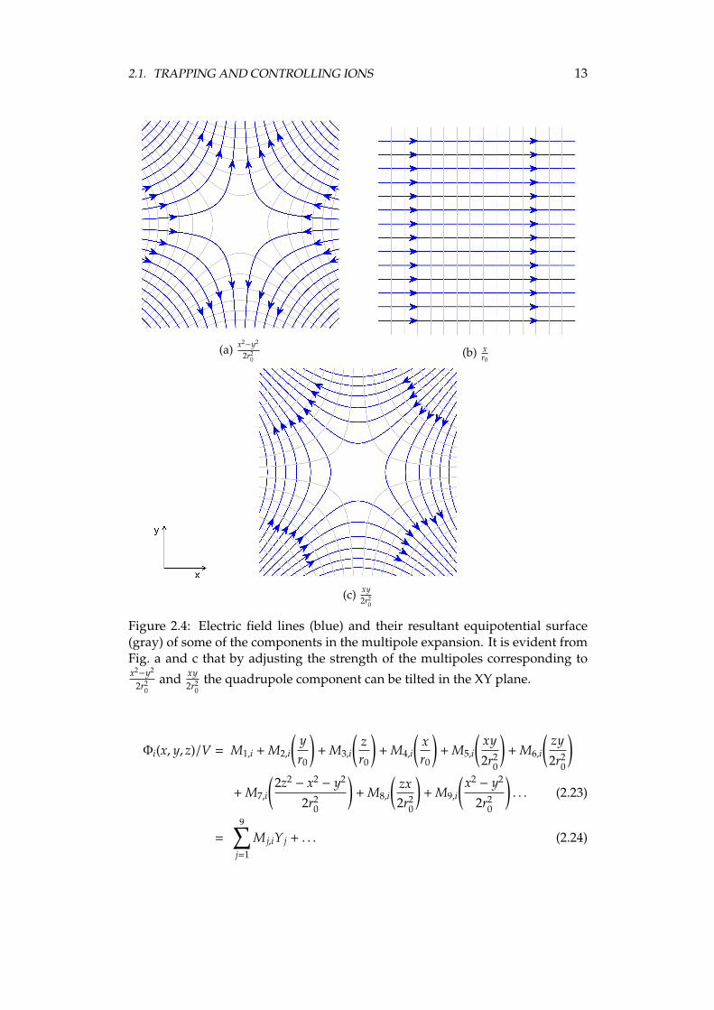
directions, respectively. Terms 5 to 9 describe the quadrupole contributions ofthe potential, which are responsible for the curvature of the potential. A pictorialrepresentation of some of the multipoles is shown in Fig. 2.4.
Mapping DC electrode voltages to the multipoles
To control the strengths of the individual multipoles of the trapping potentialthe multipoles have to be mapped on to the electrode voltages. To achieve thisthe contributions of the independent electrodes to the total potential is estimatedusing an electrostatic solver. This corresponds to the potential Φi created whena voltage of 1 V is applied to the ith electrode and 0 V to all the other electrodes,multiplied by the voltage Vi applied on it. The superposition principle dictatesthat the total potential Φ due to all the electrodes of the trap is equal to the sumof independent potentials
Φ =
N∑i=1
ViΦi
V, (2.22)
where N is the number of DC electrodes. It has to be noted that we renormal-ize Φi into a dimensionless quantity by dividing it by 1 V. This is done to preservethe units of the total potential Φ which is the summation of the products of Φi
and Vi. This is justified because Φi corresponds to the potential due to 1 V onthe ith electrode.
2.1. TRAPPING AND CONTROLLING IONS 13
(a) x2−y2
2r20
(b) xr0
(c) xy2r2
0
Figure 2.4: Electric field lines (blue) and their resultant equipotential surface(gray) of some of the components in the multipole expansion. It is evident fromFig. a and c that by adjusting the strength of the multipoles corresponding tox2−y2
2r20
and xy2r2
0the quadrupole component can be tilted in the XY plane.
Φi(x, y, z)/V = M1,i + M2,i
(yr0
)+ M3,i
(zr0
)+ M4,i
(xr0
)+ M5,i
(xy2r2
0
)+ M6,i
(zy2r2
0
)+ M7,i
(2z2− x2− y2
2r20
)+ M8,i
(zx2r2
0
)+ M9,i
(x2− y2
2r20
). . . (2.23)
=
9∑j=1
M j,iY j + . . . (2.24)

14 CHAPTER 2. THEORY
Here Y j is the jth multipole and M j,i is the coefficient describing the contri-bution of the jth multipole to the potential due to ith electrode. M j,i is a unitlessquantity that depends only on the geometry of the electrode.
The total potential in Eq. 2.22 can be written as
Φ =
N∑i=1
9∑j=1
M j,iViY j. (2.25)
Comparing 2.20 and 2.25, the coefficient vector M = M j can be written interms of the voltage vector V = Vi and the individual multipole coefficientmatrix M = M j,i as
M = MV. (2.26)
This equation can be inverted to compute the voltage vector for a given set ofM that determines the contribution of each multipole to the trapping potential
V = M−1M. (2.27)
This mapping of the multipoles to the voltages enables us to rapidly computethe set of voltages in real time, for any desired set of multi-pole coefficients.
2.2 Quantum mechanics of trapped ions coupled to lightfields
The Hamiltonian, H describing the behavior of a trapped ion interacting withthe lasers field consist of three parts [32, 30].
H = Hm + He + Hi. (2.28)
Here Hm and He describes the motional and internal state of the ion respec-tively and Hi describes the ion-laser interaction.
2.2.1 Motional Hamiltonian
In the pseudo-potential model [33], the motion of the ion is treated as a harmonicoscillator, with the Hamiltonian written as follows
Hm =p2
2m+
12
mω2r2. (2.29)
Eq. 2.29 equation can be rewritten in terms of creation and annihilationoperators as
Hm = ~ω(a†a +
12
). (2.30)

2.2. QUANTUM MECHANICS OF TRAPPED IONS COUPLED TO LIGHT FIELDS15
where
a =
√mω
2~r +
i√
2m~ωp,
a† =
√mω
2~r −
i√
2m~ωp.
(2.31)
The position and the momentum operators can be written as
r =
√~
2mω(a + a†), (2.32)
and the spread of the wavefunction can be calculated using
√〈n|r2|n〉 =
√(2n + 1)
√~
2mω. (2.33)
In a trap with secular frequencyω = 2π·1 MHz, we find that a single 40Ca+ ionin the ground state of the trap has a characteristic wavepacket size of 11 nm.
2.2.2 Two-level system
To interpret the results presented in this thesis the internal electronic structureof 40Ca+ ion is approximated as a two-level system with levels |g〉 and |e〉 withan energy difference of ~ω0 = ~(ωe − ωg). This is justified for the real ions if thedetuning of the laser from the transition of interest is much smaller than thatfrom any other transitions that might occur and if the Rabi frequency couplingthe two levels is much smaller than the detuning from those other transitions.
The corresponding Hamiltonian is given by
He = ~ωg|g〉〈g| + ~ωe|e〉〈e|
= ~ωe + ωg
2
(|g〉〈g| + |e〉〈e|
)+ ~
ω0
2
(|e〉〈e| − |g〉〈g|
).
(2.34)
By mapping the operators onto the spin-1/2 operator basis the above equationcan be written in terms of Pauli matrices as
He = ~ω0
2σz. (2.35)

16 CHAPTER 2. THEORY
2.2.3 Laser-Ion interaction
For the laser field E(r, t) = E0
(ei(k·x−ωLt) + e−i(k·x−ωLt)
), directed along the x-axis
of the trap and tuned close to a transition of the ion described as a two-levelsystems, the coupling Hamiltonian is given by
Hi =~
2Ω
(|g〉〈e|e−i(k·x−ωLt+φ) + |e〉〈g|ei(k·x−ωLt+φ)
)(2.36)
where k and ωL are the wave-vector and the frequency of the laser fieldrespectively. The Rabi frequency Ω describes the coupling strength. For a dipole-transition this is defined as (~/2)Ω = e〈g|E0 · x|e〉. The interaction Hamiltoniancan be obtained by performing the transformation Hint = U†HiU with U = eiH0t/~
Hint(t) =~
2Ωσ+e−i
(φ+η(a+a†)−δt
)+ H.C. (2.37)
where σ+ → |e〉〈g| and H.C. denotes the Hermitian conjugate of the precedingterm. Here H0 = Hm + He is the free Hamiltonian of the ion. In this equation weintroduce the Lamb-Dicke parameter, η, which is a measure of the ratio betweenthe wavelength and the extent of the ion’s ground state wave function.
η = k
√~
2mω(2.38)
Lamb-Dicke regime
The limit where the size of the motional wave function is much less than thewavelength of the light interacting with the ion is defined as Lamb-Dicke regime,i.e.
√〈n|r2|n〉 λ. Combining this with Equation 2.33, it can be observed that this
limit is satisfied when η√
2n + 1 1. In this regime the interaction Hamiltoniancan be further simplified. By expanding the argument in the exponential in Eq.2.37 to first order, we find three resonances depending on the values of δ [30].The resonance for δ = 0 is called the carrier resonance and has the form
Hcar =~
2Ω0(σ+eiφ + σ−e−iφ). (2.39)
This Hamiltonian describes the coupling of the electronic ground and excitedstates of the ion without affecting the motional state, i.e. |n〉|g〉 ↔ |n〉|e〉, with Rabifrequency of Ω0.
The resonance at δ = −ω is called the first red sideband, and the Hamiltonianreduces to the Jaynes-Cummings Hamiltonian [34], which has the form
Hrsb =~
2Ω0η(aσ+eiφ + a†σ−e−iφ). (2.40)
Assuming the ion in |g〉, this resonance reduces the motional state of the ionby one quanta while driving it between the ground and excited state, |n〉|g〉 ↔

2.2. QUANTUM MECHANICS OF TRAPPED IONS COUPLED TO LIGHT FIELDS17
(a)
(b)
Figure 2.5: (a) Schematic depicting the coupling of internal and motionalstates of the ion. When the 729 nm laser is tuned to resonance with theS1/2 ↔ D5/2 transition the population gets transferred to the excited state withouteffecting the motional state of the ion (black). If the laser is detuned to the redsideband of the transition by a secular frequency (red), the ion loses a motionalquantum while transferring the population to the excited state and similarly itgains a phonon if it is detuned to the blue sideband of the transition(blue) (b) Theresultant expected spectrum when the frequency of the 729 nm laser is scannedover the carrier and the red and the blue sidebands of a transition.
|n − 1〉|e〉. This transition can be used to entangle the motional state with theinternal state of the ion. We use this transition to perform cooling of the ionclose to its motional ground state (section 2.3.3) and to measure its motionalstate (section 2.4). The Rabi frequency for this transition is given by
Ωn,n−1 = Ω0√
nη (2.41)
Similarly the resonance at δ = +ω describes the first blue sideband transitionand the Hamiltonian has the form

18 CHAPTER 2. THEORY
Figure 2.6: The level structure of a 40Ca+ ion
Hbsb =~
2Ω0η(a†σ+eiφ + aσ−e−iφ). (2.42)
Assuming the ion in |g〉, This transition adds one phonon of secular motionwhile the ion goes to an excited state, |n〉|g〉 ↔ |n − 1〉|e〉. The Rabi frequency ofthis transition is given by
Ωn,n+1 = Ω0√
n + 1η (2.43)
A schematic of the carrier, red and blue sideband transitions, along with theresultant spectral lines is shown in Fig. 2.5
2.3 Laser-cooling of trapped ions
2.3.1 level scheme of 40Ca+
All of the experiments discussed in this thesis were carried out using 40Ca+ .40Ca+ has a simple level structure amenable for laser cooling as well as a narrowtransition allowing us to implement a qubit. Moreover, all transitions can be con-veniently driven with commercially available diode-laser systems. A schematicof the relevant energy levels of 40Ca+ with the corresponding laser wavelengthsis shown in Fig. 2.6.
The S1/2 ↔ P1/2 is a dipole transition with wavelength λ = 397 nm. The lifetime of the P1/2 level is about 7.4 ns, and the natural line width of this transitionis about 21 MHz. In our experiments we use this transition for Doppler coolingand detection of the ion. The P1/2 state can decay into the metastable D3/2 with aprobability of 7%, resulting in the obstruction of Doppler cooling and detection.To prevent this, the ion is repumped out of the D3/2 state using laser light at λ =

2.3. LASER-COOLING OF TRAPPED IONS 19
866 nm, driving the P1/2 ↔ D3/2 transition and thus emptying the metastableD3/2 state.
The state D5/2 is a metastable state with a life time of 1.2 s. We use thelong-lived S1/2 and D5/2 states as logical qubit states. The S1/2 ↔ D5/2 transitionis a quadrupole transition with wavelength λ = 729 nm and a linewidth of120 mHz. This transition is used for the coherent manipulation of the logicalqubit states. Since the natural linewidth of this transition is much smaller thanthe motional frequency of the ion, the S1/2 ↔ D5/2 transition is used to resolvethe motional modes of the ion to cool them to the motional ground state usingsideband cooling method (section 2.3.3). A dressing laser at λ = 854 nm couplesthe transition P3/2 ↔ D5/2 and ”quenches” the metastable state D5/2 by excitingion to P3/2 from which it rapidly decays back to the ground state S1/2 [35].
2.3.2 Doppler cooling
For the experiments that utilize trapped ion for quantum information processingit is necessary that the ions are cooled to the Lamb-Dicke regime (see section 2.2).This is achieved using various laser cooling methods and Doppler cooling is thefirst step in this process. Doppler cooling was first demonstrated in late 70s bydifferent groups [8, 36].
Doppler cooling involves monochromatic light with frequency tuned slightlybelow an electronic transition in an atom. The atom moving towards the lightsource experiences an increase in the frequency because of the Doppler shift. Ifthe detuning of the light frequency is adjusted such that the increased frequencyis in resonance with the electronic transition of the atom it absorbs the photon.In each absorption event, the atom loses a momentum equal to the momentumof the photon. The absorption also transfers the atom from the internal groundstate to an excited state. The atom returns to the ground state by spontaneouslyemitting the photon. Since spontaneous emission is isotropic there is no changein the average momentum of the atom. As a result the atom slows down aftermultiple absorption and emission cycles.
In case of free atoms two laser beams from opposite directions are neededto decelerate the atomic motion in one direction. However, for an ion trappedin a harmonic potential the trap reverses the ion’s velocity every half-cycle ofthe harmonic motion, so that a single laser beam can cool the ion motion [37] inthe direction of the beam. The ion trapped in a 3-dimensional Paul trap can becooled by choosing the angle of the laser beam to have a projection on all threeprincipal axes of ion’s secular motion, thereby cooling the ion in all 3 directions.
A complete analysis of laser cooling including micromotion of the ion wasderived by Cirac et.al. [38] and summarized in the review article by Leibfriedet.al. [30]. Doppler cooling is carried out using an atomic transition which hasa radiative decay rate much higher than the motional frequency of the ion,

20 CHAPTER 2. THEORY
ωi Γ, which implies the absorption and spontaneous emission of photonoccurs in a time span in which the velocity v of the ion undergoing harmonicoscillations does not change noticeably. In this limit the harmonic potential haslittle influence on the laser cooling process [39]. For a given frequency of thelaser ωL, detuning by ∆ = ωL − ω0 from the atomic transition ω0 with the Rabifrequency Ω, the radiation pressure force exerted by the laser is given by [30]
F = ~kΓρee (2.44)
where the excited state probability is
ρee =Ω2
Γ2 + 4(∆ − kv)2 . (2.45)
At lower intensities and smaller velocities, with ∆ < 0, the force describedin the equation 2.44 acts as a viscous force resulting in the cooling of the ion.Whenever a photon is emitted, the ion recoils and changes its kinetic energy.Even though the recoil kicks averages out to give a mean momentum 〈p〉 = 0, thediscrete nature of this process gives rise to a random walk in momentum space.This means that the ion is always moving and does not come to a completestop. This random walk in momentum space is what sets the lower bound of thecooling process known as Doppler limit and is given by
TDoppler =~Γ
2kB(2.46)
where kB is the Boltzmann constant.
2.3.3 Sideband cooling
Sideband cooling is a laser cooling technique employed to cool the ion beyondthe Doppler limit. Using this method the ion can be placed in the motionalground state of the trapping potential with a high probability [40, 41]. To achievesideband cooling the frequency of the laser light is tuned to address the lowermotional sideband of the transitionω0−ωi. In the Lamb-Dicke regime, forωi Γ
the spontaneous decay from the excited state will happen primarily at the carrierfrequency (see Sec. 2.2.3). This cycle results in the loss of a motional excitationevery time the atom is excited. This process is repeated until the ground state isreached, where the excitation of the red motional sideband is not possible. Anillustration of this process is presented in Fig. 2.7. The linewidth of the laser ischosen to be much smaller than the motional frequency of the ion to suppressthe excitation of the blue sideband transition.
The cooling rate of the process depends on the scattering rate. Each sidebandcooling cycle removes one phonon, hence the cooling rate is given by the productof the excited state’s decay rate, Γ and the excited level population, ρee [30],

2.3. LASER-COOLING OF TRAPPED IONS 21
Figure 2.7: Schematic describing the sideband cooling process. When the atom isexcited using the laser addressed to the red sideband transition it loses a phononand decays at the carrier frequency with a high probability. This process isrepeated until the atom reaches the motional ground state.
Rn = Γρee = Γ(Ωη√
n)2
2(Ωη√
n)2 + Γ2. (2.47)
Where Ω is the Rabi frequency, η is the Lamb-Dicke parameter and n is thequantum number of the motional state. When the ion reaches the ground state(n = 0), the cooling ceases and there will be no further excitation at the redsideband frequency. In the presence of no other heating mechanism, the low-est temperature that can be attained by the sideband cooling is limited by thenon-resonant excitations from the |n = 0〉 state. Considering the non-resonantexcitations to the nearest vibrational levels and ηΩ Γ, the steady state temper-ature is given by [30]
〈n〉 = p1 =Γ2
4ω20
(η2
η2 +14
). (2.48)
Where η is the Lamb-Dicke factor for spontaneous decay, which is differentfrom the Lamb-Dicke factor for absorption, η. This is because the emissionprocess is not limited to the same direction as the absorption process and mightalso be a different frequency. Here only excitations to the nearest motional levelare considered. Changes in the motional quantum number by two or moreare neglected since they are suppressed by a factor of η4. In the limit where
22 CHAPTER 2. THEORY
ωi Γ, off-resonant scattering becomes negligible, and the ion can be cooled tothe ground state with high probability.
2.4 Detection of the motional state
Many of the experiments discussed in this thesis require estimation of the mo-tional temperature of the ion. The wide range of temperatures in these experi-ments require us to employ different methods for temperature measurements. Inthis section we discuss the three different methods we used in our experiments.
2.4.1 Motional sideband methods
For low ion temperatures, the most accurate method to measure the averagephonon number of the ion is to map the motional state of the ion onto its internalstate, which can be measured with high efficiency. The motional temperatureof the ion can be determined by repeated measurement of this mapped internalstate of the ion.
The measurement of the motional state by mapping it onto the internal statecan be done in two ways. First method is measuring the coupling strength of thecarrier and the sideband transitions through Rabi oscillations and second methodis comparing the strengths of the red and the blue sidebands of the transition. Inthis section we describe these methods of ion temperature measurement.
Sideband comparison method
This method relies on the fact that if the ion is in the motional ground stateit doesn’t get excited when driven at the red sideband frequency, whereas theblue sideband is still present. By comparing the strengths of both excitationsthe average number of phonons can be estimated. For the ion in the electronicground state with a thermal distribution of motional states, the probability offinding the ion in the excited state, after illuminating it with laser pulse at thered sideband frequency for a duration t is given by [30]
ρRSB =
∞∑n=1
〈n〉n
(〈n〉 + 1)n+1sin2(Ωn,n−1t/2). (2.49)
Similarly the excited state population after the pulse resonant with the bluesideband is given by
ρBSB =
∞∑n=1
〈n〉n
(〈n〉 + 1)n+1sin2(Ωn,n+1t/2). (2.50)

2.4. DETECTION OF THE MOTIONAL STATE 23
These two values can be easily measured experimentally. For the excitationtime of the order of the sideband Rabi oscillation time period, the ratio of thesetwo values yields [40]
ρRSB
ρBSB=〈n〉〈n〉 + 1
, (2.51)
and the average phonon number can be estimated using
〈n〉 =ρRSB
ρBSB − ρRSB. (2.52)
This method requires the ion to be close to the motional ground state withaverage phonon number on the order of few phonons. For high 〈n〉 the strengthsof the sidebands become comparable and the method becomes inaccurate.
Rabi oscillation on motional sidebands
In the Lamb-Dicke regime the coupling strength, Ωn,n+s, depends on the motionalstate of the ion. This dependency can be used to map the motional state onto theinternal state of the ion, which can be efficiently measured.
To begin with, consider the ion in the electronic ground state, with a thermaldistribution of motional states.
|ψ〉 = |g〉∞∑
n=0
cn|n〉 (2.53)
the population of the excited states after driving the ion with a pulse resonantwith the carrier (|g〉 ↔ |e〉) for a time t is given by
ρe =12
(1 −
∞∑n=0
Pncos(Ωn,nt/2)), (2.54)
where Pn is the probability of finding the ion in motional level n. Equation2.54 is used to extract 〈n〉 from the Rabi flops on the carrier. The higher themotional excitation the more motional levels are occupied leading to a largerspread in the effective Rabi frequencies Ωn,n. A similar method can be used tofind 〈n〉 from a sideband Rabi oscillation, by using the formula
ρbsbe =
12
(1 +
∞∑n=0
Pncos(Ωn,n+1t/2)). (2.55)
The advantage of using the sideband flops for estimating the motional tem-perature over the carrier flops is that the sideband coupling is sensitive to thetemperature of that particular mode. We can thus distinguish the temperaturein the individual modes.

24 CHAPTER 2. THEORY
2.4.2 Doppler recooling method
An alternative method to measure the motional temperature of an ion is Dopplerrecooling. Unlike the previous methods Doppler recooling cannot be used tomeasure the steady state temperature of the ion. Instead, it is used to measurethe motional energy of the ion when it is higher than its Doppler limit. Comparedto the other methods this technique is relatively simple to implement and it doesnot required any ultra stable lasers.
This method takes advantage of the increased Doppler shift for an ion withan increase in its kinetic energy. When the motional energy of the ion is increasedthe Doppler shift of the laser light perceived by the ion changes, affecting it’sscattering rate, which in turn affects the fluorescence of the ion. This changein fluorescence depends on the saturation parameter and frequency detuning ofthe cooling laser.
If the frequency of the cooling laser is detuned by less than half the linewidthof the transition from the resonance, the increase in the kinetic energy results in aDoppler shift that on average makes the ion go off-resonant with the laser light.So the fluorescence of the ion decreases. When the Doppler-cooling laser beamis switched on the ion starts to cool down. This brings the ion more in resonancewith the laser leading to an increase in the fluorescence until the temperatureof the ion reaches the Doppler limit. If the cooling laser is red detuned farfrom the resonance (more than the transition linewidth), the increase in themotional energy results in a increase in the fluorescence. By monitoring thefluorescence as a function of time during Doppler cooling, we can determine theinitial temperature of the ion. A detailed analysis of the change in fluorescenceand the motional energy of the ion in the Doppler recooling process is presentedin [42].
2.5 Wiring up trapped ions
To be able to use quantum computing to solve nontrivial problems, the quantumregisters must be scaled up to accommodate large number of qubits. One strat-egy is to work with small and easy-to-control ion strings and then physicallytransport ions between different zones [43]. Other schemes transfer quantum in-formation via optical cavities [44, 45] or use long distance entanglement [46, 47].In this thesis we present a different mechanism of coupling ions in two separatetraps by allowing the charges they induce in the electrodes to affect each other’smotion [48, 49]. Related schemes have been proposed for coupling Rydbergatoms [50] and oscillating electrons [51]. In this section we present a theoreticalanalysis of this coupling mechanism.

2.5. WIRING UP TRAPPED IONS 25
(a)
(b)
Figure 2.8: a) Schematic representation of the experimental setup used for thetrapped-ion coupling experiment. A planar trap with several dc electrode seg-ments provides multiple trapping regions on the same trap chip. An electricallyisolated electrode is in proximity to ions in different trapping regions and cou-ples their motional states. b) Schematic of a wire of radius a, length L, and totalcharge λL at height H and the ion at height y above the grounded plane. In thisschematic the wire is aligned perpendicular to the plane of the paper.
2.5.1 Coupling mechanism
The basic idea of this experiment is that the quantum information stored in theelectronic degree of freedom of a single ion cooled to the motional ground statecan be mapped onto the motional degree of freedom by driving the motionalsideband of the electronic transition [6]. Thus the information is stored in super-position of the form α|0〉+β|1〉, where |n〉 is the quantum number of the harmonicoscillator describing the ion motion. This oscillating motion yields a considerabledipole moment, of order 1.8×10⁻²⁷ Cm for a 40Ca+ ion at a secular frequency of1 MHz, which can be coupled to the motion of an ion in a different trap via theirCoulomb interaction. For instance, starting with one ion in (|0〉 + |1〉)/
√2 and
the other ion in |0〉, we expect that after some time tex, the ions have exchangedstates with an acquired phase. The main idea of these experiments is to enhancethe coupling using a wire and thus provide a valuable means of interconnectingtrapped ions.
A sketch of the experimental setup is shown in Fig. 2.8a. A planar RF trap is

26 CHAPTER 2. THEORY
used to confine two ions in two different potential wells above the trap surface.Each oscillating ion induce an image charge on the electrically floating wiremounted above the trap. This results in an oscillating potential on the wirewhich is transfered to the other ion. This in turn results in a Coulombic couplingof the ions. Here we study the dynamics of the coupled ions system using theHamiltonian described in [48, 49]
Ion-wire interaction
We start this exercise with the derivation of the electrostatic coupling term undersome simplified assumptions. A schematic of the experimental setup is shownin Fig. 2.8b. We consider a metal wire of radius a and length L, situated atheight H above a (infinite) ground plane and oriented parallel to the plane. Twopoint charges, henceforth ions 1 and 2, are located at (x0,i, y0,i), i = 1, 2 and(y0,1, y0,2 < H) above the ground plane parallel to the plane passing throughthe center of the wire. The horizontal distance d, between the ions satisfiesy0,1, y0,2, H d < L. The point charges are treated here as infinitesimallysmall conductors with variable, externally set charge. Consider the situationwhere the wire is at potential V and carries a charge per unit length λ, while the’point charge’ conductors carry zero charge. Using Gauss law the voltage on thewire can be written as [26]
V =λ
2πε0ln
(2H − a
a
), (2.56)
and the voltage at the ion positions is given by
φi =λ
4πε0ln
((x0,i + xi)2 + (H + y0,i + yi)2
(x0,i + xi)2 + (H − y0,i − yi)2
), i = 1, 2. (2.57)
Here xi, yi represents the displacement of the ion i from the equilibriumposition. Green’s reciprocity theorem states that if the charge distributions ρ1
and ρ2 produce voltage configuration ϕ1 and ϕ2 respectively then [52]∫ϕ1ρ2dV =
∫ϕ2ρ1dV (2.58)
In our setup we know one of the combinations. A convenient dual situationis the one in which both point charges carry the same charge, e, while the wirecarries zero net charge and is at a potential V’. By applying Green’s reciprocitytheorem we can write down the relation as follows
λLV′ = e(φ1 + φ2). (2.59)
By substituting equations 2.57 in the equation 2.59 we can write down thepotential on the wire as

2.5. WIRING UP TRAPPED IONS 27
V′ =e
4πε0L
( ∑i=1,2
ln(
(x0,i + xi)2 + (H + y0,i + yi)2
(x0,i + xi)2 + (H − y0,i − yi)2
)). (2.60)
Given the potential, the linear charge density on the wire can be calculatedusing the formula
λ′ = 2πε0V′
α(2.61)
where α = ln((2H − a)/a
). The potential energy of each of the ion can be
written as
Ui =eV′
2αln
((x0,i + xi)2 + (H + y0,i + yi)2
(x0,i + xi)2 + (H − y0,i − yi)2
), i = 1, 2. (2.62)
The total potential energy of the system can be written as U = 1/2 (U1 + U2).The factor 1⁄2 is introduced to avoid double counting of the electrostatic energy,as described in [26, pg. 41].
For small oscillation the above potential energy can be expanded around theequilibrium position using a Taylor series
U(y1, y2) = U0 +∑
i
(∂U∂yi
∣∣∣∣∣0
)yi +
12
∑i, j
(∂2U∂yi∂y j
∣∣∣∣∣0
)yiy j, i& j = 1, 2
≈12
∑i, j
(∂2U∂yi∂y j
∣∣∣∣∣0
)yiy j =
12
∑i, j
γyiy j.
(2.63)
The coupling constant of the vertical (y) mode that enters the Hamiltonian ofthe system is
γ =∂2U∂y1∂y2
. (2.64)
As stated above, each ion is confined in an independent harmonic trap. Thusthe Hamiltonian for the coupled ion system in the presence of the floating wireconsists of two harmonic oscillator terms corresponding to each ion plus thecoupling term
H =P2
1
2m+
12
mω21y2
1 +P2
2
2m+
12
mω22y2
2 + γy1y2. (2.65)
The time evolution of the above Hamiltonian has been studied for the reso-nant case (ω1 = ω2) exactly and also in the rotating wave approximation [53]. Itwas found that the rotating wave approximation is in almost complete agreementwith the exact solution in the limit of small coupling constants (γ/mω2 < 0.1).

28 CHAPTER 2. THEORY
Another solution in the rotating wave approximation showed that full ex-change of motional states occurs only in the resonant case and for specific initialstates [54]. Let us consider the case with one ion initially in a superposition ofFock states of the form (|0〉 + |n〉)/
√2 and the second ion in the ground state. In
this case, the inverse time for state exchange of the two ions is (see appendix A)
1tex
=γ
πωm, (2.66)
where the geometry constant α was defined below equation 2.61. After timetex, the first ion is in the ground state and the second ion is in (|0〉+ e−inΘ
|n〉)/√
2,where Θ = π(mω2/γ+1/2). In experiments aiming to transfer quantum informa-tion, the presence of the acquired phase Θ poses requirements similar to thosefor preserving the coherence of the motional state of a single ion.
Another important case concerns coupling of coherent states in the resonantsystem. As shown in appendix A, we can verify that if the first ion starts out in acoherent state |µ〉, with complex amplitude µ, and the second ion in the groundstate, then after time tex the first ion is in the ground state and the second ion isin a coherent state |µe−i2Θ
〉, where Θ, defined above, describes the change of thecoherent state’s complex amplitude. This effect will be present in the classicalregime. It is due to the fact that each oscillator continues to oscillate while thestate exchange is in process and thus acquires some phase. The presence of sucha phase can most easily be observed by allowing the coupled ions to evolve fortime 2tex, so that the first ion has returned to a state |µe−i2Θ
〉.An important aspect of the above result is the extraction of the dependence
of the coupling rate on experimental parameters. The coupling rate increaseswith decreasing size of the experimental setup. In the practically interesting casewhere the ions are much closer to the wire than the trap (y0,1, y0,2 ≈ H) the lengthof the wire as well as the ion-wire distances enter mainly as 1/[L(H−y0,1)(H−y0,2)].Fig. 2.9 shows the coupling rate (1/tex) between the ions as a function of thedistance of the wire from the trap (H). Dependence on the wire radius is onlylogarithmic, included in the geometric constant α. Physically, the increasedcoupling with smaller system sizes corresponds to the fact that for ions closerto the wire the induced charges are larger, and also that for shorter wires theinduced charges are distributed over shorter distances. The scaling of tex withsystem size yields a decrease of tex by roughly an order of magnitude for adecrease of the trap size, i.e. H, y0,i , and wire length, L, by a factor of 2. Besidesthese geometrical considerations, we find an inverse dependence of the couplingrate on the ion secular frequencies, tex ∝ ω. This can be understood physically asthe motional dipole moment corresponding to each ion (∝ 1/ω) increases withlower secular frequency.
Typical parameters in the current setup are H = 170 µm, y0,i = 90 µm, L =
800 µm, a = 13 µm, ω = 2π · 2.5 MHz. With these values and for two 40Ca+ ions,

2.5. WIRING UP TRAPPED IONS 29
150 200 250 300 350 4000
5
10
15
20
25
Distance of the wire from the trap, H (µm)
Co
up
ling
ra
te, 1
/tex (
s-1
)
Figure 2.9: Plot showing the rate of coupling as a function of the distance of thewire from the trap. This plot is calculated using equation 2.66, with the lengthof the wire L = 800 µm, ion position (x0,i, y0,i) = (30, 90) µm and the secularfrequency ω = 2π · 2.5 MHz
one obtains tex ≈ 85 ms. However by reducing the secular frequency of the ionto ω = 2π · 500 kHz, the length of the wire to L = 800 µm and moving it to adistance of 50 µm from the ion, tex can be reduced by a factor of 15. We pointout that the direct electrostatic interaction between the ions is smaller than thewire-mediated term by a factor of order (H − y0,1)(H − y0,2)/L2, which for theseparameters is∼3×10⁻⁵. Thus, the direct electrostatic interaction between the ionsis negligible.
2.5.2 Sources of decoherence
While the theoretical analysis shows that there are no known fundamental ob-stacles [55], it might be surprising that the quantum information can survive thetransfer through the wire. In this subsection we discuss some of the sources ofdecoherence that contribute to the loss of the quantum information.
One source of decoherence is the dissipation of the induced current insidethe wire. Using equation 2.61, the current induced by a single ion with a lowmotional quantum number will be of order

30 CHAPTER 2. THEORY
I =eβyH∼
eβ√~ω/mH
. (2.67)
where β = 2H2/α(H2− (y0,i + yi)2) is the geometry parameter. For the pa-
rameters mentioned above, this current amounts to approximately 0.1 fA, so weexpect that it takes approximately 2 × 10⁵ s to dissipate one motional quantumon a wire resistance of 0.6 Ω, in the form of heat. Considering the inverse processby which the ion picks up motional quanta from Johnson noise in the wire theheating power P is given by
Pnoise = kT∆ν, (2.68)
where kT is the thermal energy and ∆ν is the frequency bandwidth in whichthe ion accepts the power. The time τ in which one motional quantum of energyEq = hν is generated is given by
τ−1 =Pnoise
Eq=
kT∆νhν
, (2.69)
For the values used above, the expected heating time from Johnson noiseis τ ≈ 0.1 s/quantum at room temperature, which is of the same order of theexchange time, tex. However, with the coupling rates that are feasible the Johnsonnoise is not expected to prevent the coherent transfer of quantum information.
Ion-trap experiments usually report heating rates higher than what wouldbe expected from Johnson noise [30, 56]. Experiments hint that coating theelectrode surface with contaminants has a strong influence on the observedheating [30, 56, 19]. Recent experiments have shown that the fluctuations canbe suppressed many orders of magnitude by cleaning the trap electrodes [57].Furthermore, it has been observed that cooling the trap electrodes to cryogenictemperatures (∼ 4 K) significantly reduces the heating rate of the trap. Indeed,heating rates as small as a few motional quanta per second have been observedfor ions trapped as close as 75 µm to the nearest electrode of a planar trap atthese temperatures [58, 59].
Finally, we consider the effects of a leakage current from the coupling wireto ground. The insulating material supporting the electrically floating wirehas a very high but finite resistance of the order of R ∼ 1015 Ω. In additionto this resistance the coupling wire is capacitively coupled to the ground withcapacitance of the order C ∼ 10 fF. We estimate that the RC time constant ofthis assembly is more than 100 s, which is larger than the motional couplingtimescale, tex.

Chapter 3
Experimental setup
This chapter presents a detailed description of the experimental setup whichwas used to carry out the experiments discussed in this thesis. This chapter isdivided into three sections. The first section describes the hardware requirementsfor the ion trap experiments. In the second section, we describe the RF and staticvoltages for trapping and the final section describes the software control and thepulse sequencer used to run the experiments.
3.1 General Infrastructure
We start this section with the description of the different surface traps we used inour experiments. In the next subsection we talk about the laser systems and thealignment of the various laser beams on the trap. In the last part of this sectionwe discuss our vacuum chamber and the wire assembly used for the couplingexperiments.
3.1.1 Surface traps
The experiments described in this thesis are carried out predominantly usingtwo traps named Trap-GG and Trap-A. The letters GG and A in the trap namesare not abbreviations and are chosen to identify the particular trap in a batchof about 25 traps on the chip. Both of these are planar traps with asymmetric(2:1) RF electrodes. These traps are designed and built by Nikos Daniilidis, apost-doctoral researcher in our lab. The design and the operation of these trapsare discussed in separate sections below.
The asymmetric RF design was chosen with the assumption that a tilt in theRF quadrupole will improve Doppler cooling by rotating the motional modessuch that neither of them is orthogonal to the trap surface. However, a better
31

32 CHAPTER 3. EXPERIMENTAL SETUP
understanding revealed that the pseudopotential resulting from a linear elec-trode configuration is always rotationally symmetric and hence cannot break thesymmetry required to rotate the motional modes. Instead, one can use the DCpotentials to control the orientation of the motional modes [60].
Trap GG
A detailed description of design and fabrication of Trap-GG is published inRef. [61] and a schematic of the trap including important dimensions is shownin Fig. 3.1a. This trap consist of 21 independently controlled DC electrodes.The center DC electrode is about 5 mm long, 250 µm wide and is surroundedby the asymmetric RF electrode structure. Ten equal sized DC electrodes arelocated on each side of the RF electrode structure. These electrodes are 1 mmlong and 400 µm wide. The width of the narrow and wide RF electrode are200 µm and 400 µm respectively and both electrodes are about 5.5 mm long. Allthe electrodes are separated by 10 µm gap from each other and the ground planesurrounding the electrodes. The ions are trapped 200 µm from the surface of thetrap and are displaced 15 µm from the middle of the center electrode, towardsthe narrow RF electrode.
Trap-GG is built by electroplating a 5 µm thick layer of gold on a 500 µm thicksapphire substrate. The trap is glued on a custom made stainless steel mountthat covers most of the exposed ceramic region on the CPGA to prevent theaccumulation of stray charges. The mount contains an elevated section towardsthe calcium oven to protect the trap from getting contaminated by the calcium.Quartz slides are glued below the trap to adjust the height of the trap surfacewith respect to the mount. The mount is grounded to the vacuum chamber usinga 100 nF ceramic capacitor to reduce electrical noise at frequencies of the orderof 1 MHz. A picture of the Trap-GG installed on the homemade mounted andwire bonded to the CPGA pads is shown in Fig. 3.1b.
A 100 pin ceramic pin grid array (CPGA)1 is used to mount the trap in thechamber. The CPGA is plugged in to the pin receptacles2 sandwiched betweentwo holders made of UHV compatible plastic3. The electrical connection betweenthe pads of the CPGA and the DC electrodes of the trap are made using a 25 µmgold wire-bonding wire. The wire-bonding section of each electrode is locatedabout 1.5 mm from the actual electrode as shown in Fig. 3.1a. These so-calledbonding pad is connected to the electrode through a 50 µm wide strip. Thisconfiguration is chosen for better optical access and easy wire bonding of the DCelectrodes.
1Kyocera, KD-P85989-A2Mill-Max, 0672-3-15-15-30-27-10-03Dupont, Vespel SP-1

3.1. GENERAL INFRASTRUCTURE 33
(a)
(b)
Figure 3.1: (a) The drawing showing the details of the electrode structure of Trap-GG. Dimensions of the important trap features are included in the drawing. (b)The picture of Trap-GG mounted on a custom made mount fitted on a ceramicpin grid array (CPGA). The wire bond wire used for the electrical connection ofthe trap can be seen on the edges of the trap. Quartz slides used to adjust theheight of the trap surface with respect to the surface of the mount can be seenbelow the substrate of the trap. In this setup the center electrode is grounded,but it can also be used as an additional electrode.

34 CHAPTER 3. EXPERIMENTAL SETUP
(a)
(b) (c)
Figure 3.2: a) The drawing showing the details of the electrode structure of Trap-A. The length of the RF electrode is increased to minimize it’s influence along theaxial direction. b) Schematic describing the process of angle evaporation usedin fabrication of Trap-A. The substrate is coated with 100 nm of gold at an angleof 45 so that the walls of the electrodes are partially covered with gold. c) Apicture of the Trap A glued to a CLCC.
DC and the RF voltage break down tests were carried out to determine themaximum voltage that can be applied to this trap. The test was carried out onsimilar trap produced in the same batch as the one used in the experiments.For the DC voltage the break down occurred at about 500 V. With the RF drivevoltage at 10 MHz, we could go as high as 750 V amplitude, before it broke. Atypical RF voltage used for this trap has an amplitude of 150 V and a frequencyof about 15 MHz. The DC voltages used are in the range of ±40 V.

3.1. GENERAL INFRASTRUCTURE 35
Trap A
The second trap we used in our work is named Trap-A. This trap consist of 11DC electrodes located on either sides of the RF electrodes and a center electrodelocated in between the two RF electrodes. The length of each of these 11 DCelectrodes is 200 µm and their combined width is 2.3 mm. The width of thenarrow and wide RF electrode is 100 µm and 200 µm respectively. Unlike theearlier trap the length of the RF electrode is increased to about 4 times thecombined width of the 11 DC electrodes on either sides. This is done to reducemicromotion along the axis of the trap when the ion is moved away from thetrap center in the axial direction. The width of the bonding pads is increased aswell for easy wire bonding and moved away from the trap center to ease opticalaccess. All the electrodes are separated by 5 µm gap from each other and theground plane surrounding the electrodes. The ions are trapped 100 µm fromthe surface of the trap and are displaced 15 µm from the middle of the centerelectrode, towards the narrow RF electrode. A schematic of the trap includingimportant dimensions is shown in Fig. 3.2a.
The Trap-A is fabricated by evaporating gold on quartz. 25 µm deep and5 µm wide trenches are made on the substrate that served as gaps betweenthe electrodes. The substrate is coated with 200 nm gold using double angleevaporation method so that the walls of the electrodes in the gaps are coatedwith gold to prevent the accumulation of the stray charges. Schematic describingthe angle evaporation is showing in Fig. 3.2b. The trap is glued to the ceramiclead-less chip carrier (CLCC) using UHV-compatible epoxy4 and mounted on acustom made CLCC holder made of alumina. Since the size of the is bigger thanthe center cavity of the CLCC the trap is elevated using quartz slides to clear thebonding pads on the CLCC. A picture of the trap glued to the CLCC, before anyof the wire bonds are made, is shown in Fig. 3.2c.
After the trap is installed in the chamber all the DC and RF electrodes arechecked for the connectivity from the feedthrough by touching the trap electrodeswith a gold wirebonding wire connected to the test leads of the multimeter.Typical amplitudes of the RF drive voltage are about 150 V at a frequency ofabout 35 MHz. The DC voltages used are in the range of ±20 V.
3.1.2 Optics and laser system
In this section we describe the optics and laser setup used for the photoionisation,cooling, state control and the detection of the trapped ions. All laser systemsdiscussed in this thesis are installed in a separate room and the laser light istransfered to the experimental setup using independent 22 m long optical fibers.All laser beam out-couplers except for the 729 nm laser are mounted on two
4Epotek, 353-ND

36 CHAPTER 3. EXPERIMENTAL SETUP
Figure 3.3: The schematic depicting the laser and the Ca oven alignment withrespect to the trap. The laser beams at 866 nm and 375 nm are counter propagat-ing along the axis of the trap. The Ca oven is aligned 45 to the axis of the trap.The 422 nm laser beam is combined with the 397 nm laser beam and alignedperpendicular to the oven beam. The 729 nm laser beam is counter propagatingto the 422 nm laser beam
motorized translation stages, which can be positioned with a 1 µm precisionand are controlled using a computer for the fine alignment of the beams. Theout-coupler of the 729 nm laser is mounted on a manual translation stage whichcan be moved in the direction perpendicular to the trap surface. The schematicdescribing the alignment of the laser beams with respect to the trap is shown inFig. 3.3
Photoionisation
The ion species used in our experiment is Calcium 40 (40Ca+ ), which is producedby photoionizing neutral Calcium atoms. A resistively heated calcium ovencontaining 99.99% pure Ca is used to produce the neutral calcium vapor. A5 cm long stainless steel tube sealed at one end, with an inner diameter of 1 mmand a wall thickness of about 100 µm serves as the calcium oven. To producea collimated beam of neutral calcium the tube is filled with Ca up to half thelength of the tube and the open end of the tube is directed towards the trappingregion. The tube is heated by passing a current until the tube starts spraying

3.1. GENERAL INFRASTRUCTURE 37
Ca atoms. When the Ca oven is heated for the first time after installing in thevacuum chamber, the current of the oven should be increased in small steps inorder to avoid the sudden rise in the pressure and sputter of molten calcium andother impurities from the oven. This helps in keeping the trap clean.
The Ca atoms are photoionised using a two-step photoionisation processwith the laser light at 422 nm (41S0 to 41P1) and 375 nm (41P1 to continuum).As a 422 nm laser we use a Toptica DL Pro diode laser system at 844 nm, andfrequency double it by second harmonic generation using a Beta Barium Borate(BBO) crystal inside a ring cavity setup. To produce the laser light at 375 nm,we use a free running diode laser from Nichia. To make the frequency of the422 nm laser beam resonant with the atomic transition, part of the laser lightis coupled into a wavelength meter5 and tuned close to the desired frequency.Fine tuning is done by sweeping the frequency of the laser and detecting theneutral atom fluorescence using a photo multiplier tube (PMT)6. In our setup theintensity of the 422 nm laser beam is about 60 µW and the 375 nm beam is about300 µW with a waist of about 50 µm for both the beams. The 422 nm beam isaligned perpendicular to the Ca oven to minimize the Doppler broadening. The375 nm beam is aligned such that it overlaps with the 422 nm beam only at thetrapping region. This kind of alignment is chosen to reduce the generation ofphoto-electrons by preventing photoionization of the calcium atoms where it isnot required. A schematic of the alignment of all the lasers on the trap is shownin Fig. 3.3.
Cooling and detection lasers
Doppler cooling and detection of the trapped ions is carried out on S1/2 ↔
P1/2 transition, with laser light at 397 nm. We use a Toptica DL-100 system toproduce this light. The frequency of this laser is stabilized to a line width ofabout 100 kHz by locking it to an external cavity using the Pound Drever Hall(PDH) method. For a coarse tuning of the frequency, the length of the cavityis changed by applying a voltage to the pizo transducer attached to one of themirrors of the cavity. The beam is sent through an acousto-optic modulator(AOM) in a double-pass configuration for the fine tuning of the frequency andswitching of the laser beam. The AOM has a central frequency around 220 MHzand the bandwidth of the double-pass setup is 40 MHz. The first order beamafter the double-pass is coupled to the same optical fiber carrying the 422 nmbeam using a polarizing beam cube and focused on to the trap using a 60 mmfocal length collimator 7. The waist of the 397 nm beam is about 10 µm and wereach saturation at about 1 µW of laser power.
5HighFinesse WS-76ET enterprises, electron tube 9111B7Schafter+Kirchhoff collimator 60FC-4-M60-33

38 CHAPTER 3. EXPERIMENTAL SETUP
(a)
(b)
Figure 3.4: Schematic showing the two double-pass assemblies we use to switchlaser lights and change their frequencies (a) Top and side view of the blue double-pass assembly. (b) Top view of the red double-pass assembly. The side view isnot included because the laser beam propagates in the same plane.
The efficiency of the AOM used for switching and fine tuning the 397 nmlaser is polarization sensitive. Thus we could not use the standard double-passconfiguration relying on rotation of the polarization. Instead, we use a morecomplicated setup for the double-pass using a prism. The schematic of thissetup is shown in Fig. 3.4a
A laser beam at 866 nm is used to repump the ion from the D3/2 to theP1/2 level. Like the 397 nm beam, the 866 nm laser beam is also producedusing a Toptical DL-100 system and is also locked to a similar cavity. Switchingand frequency tuning of this laser is carried out using an AOM in double-pass configuration. The AOM anti-reflection (AR) coated at this wavelength isnot polarization sensitive and we used the AOM in the standard double-passconfiguration as shown in Fig. 3.4b. The center frequency of the AOM is 80 MHzand the bandwidth of the double-pass setup is about 30 MHz. The 866 nm beamhas a waist of about 100 µm with a power of about 150 µW and is aligned along

3.1. GENERAL INFRASTRUCTURE 39
the axis of the trap.
State detection and control
The ground state S1/2 and the metastable excited state D5/2 states constitute theinternal qubit state of the ion, as described in Sec. 2.3.1. A laser beam at 729 nmcoherently drives the S1/2 - D5/2 transition . This laser light is produced using atapered amplifier (TA) amplified diode laser system. A DL Pro diode laser systemfrom Toptica, produces seed laser light of about 50 mW at 729 nm. This light isamplified to about 300 mW using a home made TA system. The frequency ofthis laser is stabilized to about 100 Hz by locking it to an ultra-high finesse cavityusing proportional-integral-derivative (PID) and fast phase locking8 methods ofstabilization. An AOM in double-pass assembly is used to control its amplitudeand frequency of the laser light. The beam is then focused on to the ions using a60 mm focal length collimator from Schafter + Kirchhoff. The waist of the beamis about 10 µm with a power of up to 7 mW at the trapping region. The beam isaligned at a 45 to both x and z axes of the trap, as shown in Fig.3.3.
The life time of the excited, metastable D5/2 state is about 1.1 s [62]. Aquenching laser at 854 nm is used to speed up the spontaneous decay of theion to the ground state via the P3/2 state. This light is produced and frequencystabilized similar to that of the 866 nm laser and is coupled into the same opticalfiber carrying 866 nm light. The waist and power of the 854 nm laser beam issimilar to that of the 866 nm laser beam at the trapping region.
Detection and imaging
The fluorescence emitted by the ions is collected and focused on to the photo-multiplier tube (PMT) using a custom made objective9 with a focal length of67 mm and NA of 0.28. A 90:10 beam splitter in front of the PMT splits off 10%of the light for imaging the ions on a CCD camera10. Both devices are fitted withnarrow band pass filters11 to select for 397 nm light.
3.1.3 Vacuum chamber assembly
The ion trap experiments are carried out in an ultra-high vacuum (UHV) chamberat a pressures below 10−11 mbar to prevent the collision of ions with backgroundgas molecules. An isometric view of our UHV chamber assembly is shown inFig. 3.5. The vacuum chamber is a 6” stainless steel spherical octagon fromKimball Physics, which has eight equally spaced horizontal ports and two 6”
8Toptica FALC 110 module9Silloptics, Germany
10Andor, iXon DV885 JCS-VP11Semrock FF01-377/50-25 and FF01-417/60-25

40 CHAPTER 3. EXPERIMENTAL SETUP
Figure 3.5: Schematic of our vacuum chamber assembly. The Ca oven thatis missing in this picture is connected to the feedthrough opposite to the RFfeedthrough, via a flexible bellow for alignment of the oven. In future setups theion-pump will have to be moved to the position of the angle valve in an attemptto reduce the current high values of stray magnet fields on the order of 20 G.
vertical ports. The top 6” port is used for imaging. Four of the horizontal portsare fitted with viewports for optical access. Two horizontal ports are fitted with8 pin high power feedthroughs for oven and RF voltage supply. One horizontalport is fitted with a twin 25 pin D-sub connector for DC voltage supply. Theone remaining horizontal port is fitted with a six way cross, which attachesthe vacuum chamber to the ion pump12, ion gauge, angle valve and a 12 pinelectrical feedthrough to supply the voltage for piezo actuators holding the wire.A titanium sublimation (Ti-Sub) pump13 is attached to the bottom 6” port usinga zero length reducer and a three way cross.
To achieve the ultra-high vacuum, the vacuum chamber assembly should bethoroughly checked for leaks. Once the chamber is free of leaks it is baked at150 C while pumping with the turbomolecular pump until the pressure insidethe chamber drops well below 10−7 mbar. After the bake the ion gauge and theion pump are switched on. The Ti-Sub pump is heated by passing 50 A of currentthrough one of the filaments for one minute. This is done 4 to 5 times with aninterval of half an hour between each run. The angle valve is closed and theturbomolecular pump is disconnected from the angle valve. Now the pressureinside the chamber should be below 10−10 mbar. The Ti-Sub pump should beswitched on 2-3 times every day till the pressure stops going down.
12Varian, StarCell 20L/s13Varian, 9160050

3.1. GENERAL INFRASTRUCTURE 41
Figure 3.6: Schematic showing the first wire assembly. The earlier version ofthe wire holder is made using Macor (a machinable glass ceramic), but wasreplaced by a stainless steel holder fearing the build up of stray charges on theinsulator. The wire used for the experiments was a 25 µm gold wire bondingwire connected between the two prongs of the frame. This frame was mountedon a stack of PZT stages to control its alignment in the experiment.
3.1.4 Coupling wire assembly
To carry out the experiment of wire mediated coupling of two ions, described inSec. 2.5, we need a metallic wire which has a very low resistance and is electricallywell insulated from the surroundings. We should be able to control the positionof the wire during the experiment to avoid contamination of the wire duringloading. It is important that the natural vibrational frequency of the wire is notclose to any of the secular frequencies of the ion to prevent motional heating ofthe ion. In this section, we describe the two wire assemblies we used to studythe ion wire interaction.
Single wire assembly
The first version of the wire assembly consists of a 1 cm long, 25 µm thick goldwire-bond wire held using a frame made of a machinable glass ceramic materialcalled Macor14. A schematic of this assembly is shown in Fig. 3.6. In this setup theceramic portion was completely exposed and was getting electrically charged,which resulted in the instability of the trapped ion. To overcome this problem,the second version of the wire holder was manufactured using stainless steelinstead of Macor, with a small ceramic tip to keep the wire insulated from theframe.
14Corning Inc.

42 CHAPTER 3. EXPERIMENTAL SETUP
(a) (b)
(c)
Figure 3.7: (a) Schematic depicting the evaporation setup of the three wireassembly. When this structure is evaporated on both sides with gold, the stainlesssteel rods cast a shadow on the glass fibers, creating a insulating region duringevaporation. The wire used for the experiments is the electrically floating portionin between the two insulating regions. (b) The final assembly with three floatingwires just before it is mounted on the PZT stacks. (c) The complete assembly.along the trap, mounted inside the vacuum chamber.
The wire holder is mounted on a stack of 4 piezo driven nano-positioningstages from Attocube. The bottom two linear translation stages are used toposition the wire in the vertical (y) and horizontal (x) directions. The top twoare rotational stages which are used to make the wire parallel to the trap surfaceand to move the wire away from above the trap. These stages use a stick-slip method [63] to achieve the displacement. Independent sawtooth voltagesto operate the stages are supplied from a control unit through a 9 pin D-Subconnector. The holder is electrically insulated from the base of the stages, whichallows us to apply a voltage on the wire assembly. The length of the piezo stackis about 10 cm, to match the height of the trap with the wire, an extender isconnected to the bottom 6” port, of the octagon chamber.
Multiple wire assembly
The newer version of the wire assembly consist of three wires. The couplingwires in this assembly are gold coated, 25 µm thick glass fibers. To produce the

3.2. VOLTAGE SOURCE 43
wires, the three glass fibers are glued to a stainless steel square frame about 1 cmwide and 1 mm thick using UHV epoxy (cf. Fig. 3.7b). Two pairs of 75 µm thickrods separated by 800 µm, are placed on either sides of the wire to shadow thegold coating, as shown in Fig. 3.7a. The frame along with the wires is evaporatedwith gold to a thickness of 100 nm. The shadow rods are removed and the frameis left with 3 electrically floating wires, each 800 µm long, held in place by goldcoated fibers on both sides. One side of the frame holding the wires is madeto be electrically insulated from the other side for measuring the continuity ofthe wires. This yields useful information on whether the center wire might beelectrically connected to the frame.
The wire frame is mounted on the same set of piezo stacks described inSec. 3.1.4. A picture of the wire frame mounted in the vacuum chamber, alongwith the surface trap is shown in Fig. 3.7c. Even though the evaporation methodresults in a wire with a 12-fold increased resistance as compared to a solid goldwire of the same diameter, this method was preferred because it allowed us tomake the wire as short as 800 µm without compromising optical access.
3.1.5 Magnetic field coils
In an ion trap setup, magnetic field coils are essential for compensating straymagnetic fields and to define a quantization axis for the experiment. In oursetup we found that we have a large stray magnetic field of the order 20 Gaussalong the x direction of the trap. To compensate for the magnetic field along thedirection of the 729 nm laser beam, we use a 1200 turn coil with a radius of 10 cm.A current of about 1 A is passed through this coil. For the direction perpendicularto the 729 nm laser beam, which is also our direction of quantization, we use2 coils on each side of the vacuum chamber. One coil has 400 turns and aradius of 3 cm and the other one has 200 turns and a 15 cm radius. A currentof about 3 A is passed through these coils, which produces a magnetic field ofabout 10 Gauss to cancel the stray magnetic field. The combination results inquantization magnetic field of about 3.5 Gauss. A schematic of the magneticfield coil setup is shown in Fig.3.8.
3.2 Voltage source
This section describes the generation of RF and DC voltages required for trappingof ions as well as the stable current supply required to produce the quantizationmagnetic field.

44 CHAPTER 3. EXPERIMENTAL SETUP
Figure 3.8: Schematic showing the alignment of the magnetic field coils withrespect to the laser beams and the vacuum chamber. Because of the constraints inthe space around the vacuum chamber two coils are used for partial cancellationof the magnetic field along the axis of quantization, while one big coil is usedin the direction perpendicular to it. Since the stray magnetic field in the thirddirection is negligible, no coil is used in this direction.
3.2.1 RF Voltage
A 35 MHz radio frequency (RF) voltage with an amplitude up to 200 V is usedas a drive for trapping ions. A Rohde & Schwarz SMB100A frequency generatorproduces the RF signal, which is amplified using a Minicircuits ZHL-1-5W am-plifier. This RF voltage is stepped up using a helical resonator [64] and connectedto the RF feedthrough of the vacuum chamber. A helical resonator is a quarterwave resonator that converts the RF power to a high voltage low-current signal.It is an LC circuit consisting of a helical coil placed inside a conducting cylindri-cal can. The resonance frequency of the resonator can be changed by changingthe geometry and number of turns of the coil. The RF signal is coupled in to theresonator using a small antenna coil placed inside the helical coil [65]. The in-coupling is tuned by changing the position of the antenna coil while monitoringthe reflected signal. Good in-coupling is achieved when the reflected power isless than 2 orders of magnitude of the input power. The inductive coupling intothe helical resonator is chosen to keep the helical resonator electrically isolatedfrom the RF amplifier and source. The helical resonator couples to other metallic

3.3. EXPERIMENTAL CONTROL 45
objects nearby, such as chairs. This resulted in amplitude fluctuations in RFdrive when those objects are moved. To prevent this, the resonator along withthe amplifier is placed inside a 2 mm thick aluminum can which is grounded tothe optical table.
A rough calibration of the output voltage of the helical resonator to theinput power is done in the beginning, using a capacitive divider. For day-to-day operations the resonance of the helical resonator is monitored using adirectional coupler by connecting the output end of the directional coupler tothe RF amplifier and the input end to the helical resonator. The best estimateof the voltage applied is obtained by measuring the radial secular frequency ofions.
3.2.2 DC Voltage
Stable, tunable, ultra low noise static voltages are applied to all the DC electrodesfor trapping and control of the ion. To achieve this we built a 24 channel digitalanalog converter (DAC) board, controlled by a field-programmable gate array(FPGA). Each DAC channel has a range of ±10 V with a resolution of 32 bit.The output of the DACs are amplified using a OP-AMP amplification circuit toachieve a range of ±40 V. The amplified voltages are calibrated for each channelfor the whole range and the corrected voltages are used for the experiments.
3.3 Experimental control
Efficient running of the experiment requires us to simultaneously switch andvary multiple parameters with a high degree of accuracy. To achieve this weuse automated scripts running on computers to control various hardware com-ponents and data acquisition. The earlier version of our experimental controlwas based on LabView, supported by a python back-end. This was effectivefor the experiment in the initial stages, but as the complexity of the experimentincreased the core structure of the program became very complex and resultedin frequent failures. The intricate nature of the program also made it very hardto modify or troubleshoot the process.
These complications forced us to switch to LabRAD to control our experi-ments. LabRAD is an open source protocol, developed by the Martinis groupat University of California, Santa Barbara (UCSB). Using LabRAD, the exper-imental control can be written as collection of codes, called servers to controlindividual hardware components. This decentralized nature of LabRAD makesis possible to run the servers in multiple machines connected using TransmissionControl Protocol (TCP), allowing for a high modularity. The modular nature ofthis software also makes trouble shooting relatively easy.

46 CHAPTER 3. EXPERIMENTAL SETUP
The software control for our experiment is located in three independentcomputers, which are connected using ethernet and communicate via TCP. Theschematic of the various hardware components used in our experiment and theirconnection to the control software is shown in Fig. 3.9.
The Graphic User Interface(GUI) for our experimental control is located in themain computer which communicates with the most important hardware used inour experiments such as the pulse sequence generator. A detailed description ofthe experimental control based on LabRAD is given in Michael Ramm’s thesis[66].
The pulse sequence generator, or in short Pulser, is a field-programmablegate array (FPGA) based hardware that generates the TTL pulses required totrigger the hardware components. It also controls the frequency, amplitudeand phase of various Direct Digital Synthesizers (DDS) used to control the laserfields. Apart from producing pulse sequences the pulser can also be used for theacquisition of digital signals, which we use to read our PMT signal. The Pulsercan also be used to control the DAC for the generation of DC voltages requiredfor the trapping. However, we use a second scaled down version of the Pulserfor the DC voltages in order to free up some channels in our main pulser. ThePulser communicates with the computer via TCP. A detailed description of thishardware give in Thaned Pruttivarasin’s thesis [67].
Most experiments sensitive to magnetic field noise can be improved by syn-chronizing them to the frequency of the alternating current (AC) line. To accom-plish this, the line signal is stepped down and converted to a square pulse andfed into the pulser. This square pulse is used as a trigger for all the experiments.
The main experimental computer also controls two frequency generators,which are connected through a serial port. These signal generators are usedto produce the drive frequency for the trap and excitation frequency for themicromotion compensation described in the chapter 4.
The second computer in our setup is mainly used for the camera acquisition.This is important for the alignment of the laser beams on the trap and to findthe distance of the wire from the ion. This computer also controls the motorizedtranslation stages used to change the position of the laser beams and the piezostages supporting the wire. The server controlling the piezo communicates withthe main computer through the TCP connection as shown in Fig. 3.9.
The third computer we use is situated in the laser room and is shared by allthe experiments in our lab. This computer monitors the frequency of the lasersby sequentially switching the laser beams going into the wavemeter using amultiplexer. This computer is also used to change the frequency of the laser lightby changing the voltage of the piezos connected to the locking-cavity mirrors.

3.3. EXPERIMENTAL CONTROL 47
Figure 3.9: Schematic showing various components of the experimental controldistributed over three computers.The DAC control that supplies the voltages tothe DC electrodes, The Rohde and Schwarz frequency generator that producesthe radio frequency for the trap drive and the pulsar unit that generates the pulsesequence of the experiment are connected to the main computer. The cameraused to monitor the ion is connected to the camera computer. This computer isalso used to control the motorized translation stages that move the laser beamsand the PZT stages that move the wire. A third computer in the laser roomcontrol the DACs that supply the DC voltages for tuning the external cavitiesused for locking the laser frequencies. This computer is also connected to thewavemeter that monitors the frequencies of the laser.


Chapter 4
Stray electric field sensing andcompensation
For a reliable operation of segmented ion traps a complete control over theelectrostatic environment in the trapping region is necessary. To achieve this anaccurate model of the potential created by the trap electrodes is required. Butthe stray electric field created by unaccounted charges resting on the insulatingregions around the trap cannot be included these simulations. These stray fieldscause the ion to displace from the RF null, resulting in a so-called micromotion[68]. In this chapter we discuss how to measure and minimize this micromotion.We also describe how compensation of the micromotion at various positions onthe axis of the trap can be used to map the electric field along the axis. Weconclude this chapter by discussing various possible sources for the observedstray charges.
4.1 Micromotion in ion traps
In an ideal Paul trap ions are confined to the position where the electric field dueto the oscillating RF drive is zero. But in a typical ion trap any additional electricfield pushes the ion from the center of the RF quadrupole away. Thus the ionexperiences an oscillating force from the RF-drive causing so-called micromotion.Unwanted effects of micromotion include spectral broadening of the atomictransitions via the Doppler effect and heating of the ion motion due to noisepresent in the RF drive [19]. To avoid those effects, it is important to place theion close to the RF-node.
Different techniques exist for detecting micromotion [68]. The photon corre-lation method relies on correlating the ion fluorescence to the phase of the RF
49

50 CHAPTER 4. STRAY ELECTRIC FIELD SENSING AND COMPENSATION
Figure 4.1: Schematic showing the side view of the alignment of the laser beamon the trap. The laser beam does not have a projection on the ion oscillationalong the y direction unless the laser beam is made to bounce off the surface ofthe trap, which can result in high stray light and the charing of the trap.
field [69]. In the resolved sideband method [70] the sidebands of a narrow atomictransition are compared with the carrier transition to estimate the modulationindex. Both methods are widely used to detect micromotion in 3D traps. How-ever, neither of the methods can be easily extended to surface Paul traps becausethey directly use the Doppler shift induced by the ion motion. This requires thelaser beam to have a projection on all three directions of the ion motion. In thecase of surface traps, the geometry typically limits the laser alignment to be inthe plane parallel to the trap surface (see Fig. 4.1). For such laser alignments, theDoppler effect due to motion perpendicular to the trap surface vanishes makingit very difficult to detect such micromotion.
4.1.1 Principle of compensation
In this section we present a method of micromotion compensation that doesnot depend on the detection of the micromotion using the directly associatedDoppler shift. Instead, we test if the voltage applied to the RF electrodes effectthe ion.
If the ion is displaced from the center of the RF quadrupole, any voltageapplied on the RF electrode applies a force on the ion. If that force has a projectionalong a secular motion and if it has a frequency component that is resonant withone of the secular frequencies of the ion, the ion motion is excited resonantly[71, 72]. Experimentally, we found that the resulting large oscillation amplitudesof each of the three secular motions can be detected very efficiently as a drop inion fluorescence. The dynamics of ion fluorescence as a function of its vibrationalenergy in the presence of the cooling laser is described in Ref. [42]. Micromotioncompensation is achieved by moving the ion until it does not get excited whenthe external drive frequency is resonant with any of the ion’s secular frequencies.The DC electrode voltages are tuned to move the ion in all the three directions.

4.1. MICROMOTION IN ION TRAPS 51
The results of this experiment are discussed in the following subsections andare published in Ref. [25]. This method is also being used by the NIST [73] andOsaska [72] ion trap groups.
4.1.2 Implementation
First a coarse compensation of micromotion is achieved by changing the RFdrive voltage and monitoring the ion displacement. When the RF drive voltageis increased the radial confinement of the ion gets stronger and the ion movestowards the RF null. The electrode voltages should be adjusted such that the ionstops moving when the RF drive voltage is varied. The displacement of the ionin the x direction is detected using the camera (see Fig. 4.1). In the y directionthe displacement can be detected by monitoring the change in the fluorescencelevel when the ion moves in and out of the laser beam. To achieve the maximumsensitivity, the laser beam is moved in the y direction such that the intensity ishalf the maximum, to increase the laser intensity gradient. The ion is placedwithin 1 µm from the RF null using this method.
The micromotion in the x direction is further reduced by monitoring thelinewidth of the S1/2 ↔ P1/2 transition of the ion. If the ion is experiencingmicromotion, sidebands at the drive frequencies appear on either sides of theatomic transition. This can be used for the detection of the micromotion. Tominimize the micromotion, the intensity of the laser is kept at half the saturationof the transition. The laser frequency is red detuned so that the fluorescencedrops to one-third of the saturation value. The electrode voltages are adjustedto move the ion and reduce the fluorescence of the ion. This is repeated until theline width cannot be reduced any further.
After a coarse compensation of micromotion is achieved using the abovemethods, we proceed with the method of compensation as outlined in Sec. 4.1.1.The schematic of the experimental setup is shown in Fig. 4.2. The bandwidth ofthe helical resonator used to generate the high voltage for the RF-drive does notallow us to excite the ion at the frequency ωi, so instead of exciting the secularfrequency ωi directly, we excite the ion at a frequency ΩRF ± ωi. The RF signalrequired to excite the ion is supplied by a Rohde & Schwarz frequency generator.This signal is mixed with the RF drive ΩRF before it is amplified and stepped upusing the helical resonator as explained in Sec. 3.2.1. This produces sidebandsat ΩRF ± ωi on the drive RF voltage. When ωi is scanned around the secularfrequencies of the ion, the side bands on the drive voltage become resonantwith the micromotion sideband of the ion and the ion gets excited, resulting ina reduction in the ion fluorescence [71, 74]. One of the important requirementsof this method is that the helical resonator has a large enough bandwidth toapply the secular sidebands of the RF drive. The resonator used in our setup hasbandwidth of about 270 kHz and allows compensation at secular frequencies of

52 CHAPTER 4. STRAY ELECTRIC FIELD SENSING AND COMPENSATION
Figure 4.2: Schematic showing the electrical connections for the implementationof micromotion compensation using the excitation method. The RF signal at themicromotion sideband frequency is mixed with the RF drive for trapping andamplified before connecting it to the step-up resonator. The ion displaced fromthe RF null gets excited in the direction of the motional mode corresponding tothe sideband frequency applied.
2 MHz.
The GPIB cable used to connect the excitation frequency source to the com-puter has a response time of few 100 ms. Continuous excitation of the ion forsuch duration at the frequency resonant with the secular sideband of the micro-motion of the ion often results in the loss of ion. We overcame this problem byswitching on and off the excitation signal by sending it through a switch con-trolled using a square wave generator at a frequency of 1 kHz. The frequenciesof the detection and repump lasers are kept close to their respective transitionsof the ion, to maximize the sensitivity [71]. For the experiments presented inthis section the frequency of the 397 nm laser is detuned by 3 MHz to the red,compared to the natural linewidth of about 20 MHz of the S1/2 ↔ P1/2 transition.
Total compensation of micromotion is achieved by compensating the micro-motion in x and y directions iteratively. First the compensation of micromotionin the x direction is achieved. For this the excitation frequency is scanned aroundthe secular frequency ωx corresponding to the x direction. When the frequenciesare in resonance the ion fluorescence drops. A typical frequency scan resultingin a drop in the ion fluorescence is shown in Fig.4.3. Empirically we observedthat a good fit for the drop in the fluorescence is achieved by analyzing it usingthe following function.

4.1. MICROMOTION IN ION TRAPS 53
Figure 4.3: Plot showing the drop in the ion fluorescence when the frequency ofthe excitation signal is in resonance with the secular sideband of the micromotionof the ion, which is not micromotion compensated. The data is fitted with aninverse exponentiated quartic function described in the equation 4.1, empiricallychosen for an accurate estimate of the drop in fluorescence.
F(ωs) = Fs − d· exp(−
(ωs − ω0)2
(w2)2 −(ωs − ω0)4
(w4)4
). (4.1)
where F(ωs) is the ion fluorescence at excitation frequency ωs and ω0 is thesecular frequency of the ion. The power of the excitation signal is adjustedsuch that the dip in the fluorescence signal is not saturated. Now the electrodevoltages are changed such that the electric field minimum at the ion movespredominantly in the x direction, resulting in a displacement of ion in the xdirection. If the depth of the dip is lower than the previous scan, micromotionis reduced. This process is repeated until the dip in the fluorescence disappears.If the dip in the frequency scans is not visible for more than one ion position,the scans are repeated with a higher power. These sets of frequency scansare repeated with different ion displacement ranges until the best resolution inthe displacement is reached. After the micromotion is compensated in the xdirection, the ion is kept at a compensated position along the x direction and thesame procedure is repeated for the compensation along the y direction.
The results presented in this chapter were obtained with Trap-GG describedin Sec. 3.1.1. The outer electrodes 1, 2, 3, 9 and 10 on both sides of the RF alongwith the center electrode were grounded. The ion was trapped in the middle of

54 CHAPTER 4. STRAY ELECTRIC FIELD SENSING AND COMPENSATION
electrode 6. To move the ion in the y direction, a constant voltage was addedto all DC electrodes. The displacement of ion in the x direction in achieved byadding and subtracting a constant voltage to the voltage on the electrode 6, oneither side of the RF, keeping rest of the DC voltages constant.
Results and discussion
The result of this experiment is plotted in the Fig. 4.4. Fig. 4.4a and 4.4b showthe change in the depth of the dip when the excitation frequency is in resonancewith the micromotion sideband of the ion ΩRF + ωx and ΩRF + ωy respectively,as a function of ion position in x and y direction. For gray regions in Fig. 4.4athere exist no data because the excitation would drive the ion out of the trap.Cross sections of the 2D plots are plotted in Fig. 4.4c and 4.4d. The plots showsthe change in the strength of the excitation when the ion is moved along x andy direction respectively. The energy gained is expected to be proportional to thesquare of the electric excitation field [56]. This is consistent with the data whichfits well with a parabola, as the excitation of the quadrupole field is linear in theion position.
The accuracy of the ion position is estimated by calibrating the displacementof the ion as a function of the applied correction voltages. In the x direction theCCD camera is used to determine the displacement. In the y direction the dis-placement is determined using the position of the laser beam yielding maximumfluorescence. These values were verified by modeling the displacement of theDC minimum with variation of the compensation voltages. By translating theapplied voltage into an actual displacement, we determine an accuracy of about50 nm in the x direction and 300 nm in y direction in positioning the ion at theRF minimum. This corresponds to excess micromotion amplitudes of 6 nm and40 nm in these respective directions. The accuracies could be further improvedby increasing the excitation voltage and decreasing the frequency detuning ofthe detection laser from resonance [42].
So far in this section we have discussed the micromotion of the ion arisingdue to the stray charges, which can be compensated by applying counter electricfields using the DC electrodes. But the micromotion can also arise due to thegeometry and/or the electrical connections of the trap. In a typical trap setup thedrive voltage applied on the RF electrodes gets capacitively coupled to the DCelectrodes. Since the quadrupole formed by the DC electrodes is different fromthe one formed by the RF electrode, the oscillating voltage picked up by the DCelectrodes results in the displacement of the RF null. If the picked up voltage hasa different phase than that of the RF drive the position of the RF null oscillateswith the frequency of the RF drive. This induces a micromotion depending ofthe phase difference of the pickup voltage. Since there is no region where theelectric field created by these two voltages are zero throughout the oscillation

4.2. ELECTRIC FIELD SENSING 55
(a) (b)
(c) (d)
Figure 4.4: (a) and (b) plots the depth of the dip as the function of ion positionin the x and y directions, when the ion is excited with the frequencies ΩRF + ωxand ΩRF + ωy respectively. The gray area in the plot (a) is the region withoutdata because the excitation might drive the ion out of the trap. Darker color inthe plot indicates a smaller dip value. (c) and (d) are the cross section of (a) and(b) respectively, fitted with a parabola.
cycle, the micromotion arising from this effect cannot be compensated.
4.2 Electric field sensing
In this section we explain how the compensation of micromotion can be extendedto map the electric field along the axis of a surface trap. This information ofthe electric field over an extended region of the trap is very important for ionshuttling experiments and can be very useful in determining the mechanism ofcharging on surface traps.
The essential part of the stray field estimation is to perform micromotioncompensation as described above. After the compensation parameters have beendetermined, we measure the ion position along the z direction using the CCDimaging system. The values of the dc voltages at the compensated configuration

56 CHAPTER 4. STRAY ELECTRIC FIELD SENSING AND COMPENSATION
and the ion position are then input to a minimization algorithm. The algorithmfinds the corresponding stray electric field at that position. We performed thistype of analysis over an extensive region along the axis of the trap and theresults are plotted in Fig. 4.5. Fig. 4.5a shows the three components of the strayelectric field Ex, Ey, Ez plotted in red, green and blue, respectively along withits magnitude |
−→E | plotted in black. Since the scale of the stray electric field is
too large to see the error bars a closer view of each of the curves is plottedseparately in Fig. 4.5b. It is evident from the plot that the stray electric fieldvalues closer to the middle DC electrode of the trap are higher than the fieldvalues at the outer DC electrodes. The results of this measurement is analyzedin the subsection 4.3.1.
The accuracy of this measurement scheme was mostly limited by the un-certainty in the determining of the absolute position of the ion along the axisof the trap. This uncertainty arises due to the imprecision in the alignment ofthe microscope objective used for imaging with respect to the trap and from thesize of the trap features used to determine the position of the ion on the trap.This uncertainty was estimated to be ±2.5 µm which translates as an inaccuracyof (δx, δy, δz) = ±(5.5, 3, 15) V/m in the measurement of the stray electric field.This was a systematic error, leading mainly to an offset of the entire curve. Theprecision of the stray electric field measurement was limited by the imperfectionin the compensation of the micromotion of the ion. This leads to an uncertaintyof ±0.4 V/m in the x direction and ±2.5 V/m in the y direction.
The third factor limiting the measurement of the stray electric fields was theaberration of the imaging system. This introduces an uncertainty in determiningthe ion position at a given voltage settings with respect to the previous settingsas the ion was shuttled along the axis of the trap. This introduces an uncertaintyof±0.1 µm, which leads to an imperfection of±(2, 4, 0.5) V/m in the measurementof stray electric field. All these above mentioned imperfections sum up to anuncertainty of (δx, δy, δz) = ±(8, 10, 16) V/m. However all these imperfectionscan be further improved.
These measurement were performed on the trap-GG. The detailed descrip-tion of the trap is presented in Sec. 3.1.1. The voltages used in the transport of theion along the axis of the trap were supplied by Prof. Ferdinand Schmidt-kaler’sgroup, then at University of Ulm, now at University of Mainz. The voltage fileconsists of about 300 sets of voltages. Each set consists of the voltages for allthe trap electrodes required to trap the ion at a certain point along the axis ofthe trap. When the voltages on the electrodes are switched to the values in theneighboring subset, the ion shifts to a new position, about 7 µm apart. For ourexperiment the ion was shuttled in steps of 15 µm to 30 µm, as plotted in Fig. 4.5.
In addition the secular frequencies at each position along the axis of the trapare estimated using the electrostatic solver. Since the radial trap axes are tilted we

4.2. ELECTRIC FIELD SENSING 57
(a)
(b)
Figure 4.5: (a) Stray electric field along the axis of the trap. The three componentsEx, Ey, Ez are plotted in red, green and blue, respectively. The magnitude |
−→E |
of the stray field is plotted in black (b) Since the scale of the stray electric fieldis too large to see the error bars a closer view of each of the four curves areplotted separately. The solid curves on the two sides of each curve correspondto the possible systematic offset arising from the uncertainty in the absolute axialposition, as described in the text.

58 CHAPTER 4. STRAY ELECTRIC FIELD SENSING AND COMPENSATION
1000 1500 2000 2500 3000 3500-1
-0.8
-0.6
-0.4
-0.2
0
0.2
0.4
0.6
0.8
1x 10
7
Axial position Z (µm)
Curv
atu
re (
V/m
2)
Figure 4.6: The curvature of the stray electric field along the axis of the trap.Thesolid line is the estimated gradient using the change in the stray field and the dots(•) represent the curvature of the stray field as determined from the differencebetween measured and estimated secular frequencies
determine the radial secular frequencies using a two-dimensional polynomial fitin the xy plane. The agreement between the experiment and the measurementwas better than 4%, corresponding to a disagreement of 20 kHz for an axialfrequency of 500 kHz and 30 kHz for redial frequencies between 1 to 2 MHz.We attribute these disagreements to details of the trap geometry that were notincluded in the simulations and the unknown curvature of the stray electric field.Only the spatially inhomogeneous part of the stray field was responsible for thediscrepancy between the estimated and the measured electric field since theelectrostatic stray fields are compensated and included in the simulations. Weused this discrepancy induced in the trap frequencies to estimate the curvaturein the stray field and compared it with the curvature of the stray field estimatedusing the change in the stray field. The results are plotted in Fig. 4.6. The datapoints in the plot denoted by dots (•) represents the curvature of the stray fieldas determined from the difference between measured and estimated secularfrequencies. The solid line is the estimated gradient using the change in thestray field. The values from both the methods match very well. For the resultsdiscussed in this section the electrostatic modeling of the trap was carried outusing a boundary element method solver CPO 1.
1www.electronoptics.com

4.3. POSSIBLE SOURCES OF THE STRAY ELECTRIC FIELD 59
4.3 Possible sources of the stray electric field
In this section we discuss some of our observations and experiments that helpedus get an idea about the source and location of the charges causing the strayelectric fields. The first subsection analyzes the source and the pattern of theelectrical stray field we discussed in Sec. 4.2. In the latter part of this section wepresent some of our experiments to identify the sources, locations and cure forthe stray charges.
4.3.1 Abrupt change in the stray fields
The effect of stray field was first observed on the Trap-GG. A quantitative estimateof stray field and the process of its measurement is presented in Sec. 4.2. Thesemeasurements were carried out over a period of several months. In the firstcouple of months of trap operation we monitored the stray field only at onetrapping position close to the center of the trap. During this time we foundthe mean magnitude of the field to be 47 V/m with a standard deviation of52 V/m. After about two months of trap operation the ion pump pumping thevacuum chamber stopped working due to an interlock-failure. During this timethe pressure inside the chamber went up to 10−7 mbar. The ion pump remainedswitched off for about a week during which the chamber was not used for anyexperiment. After a week the vacuum was restored by turning on the ion pumpand firing the Ti-Sub pump for a few times.
The new stray field values measured after this incident were about an orderof magnitude higher than the field measured earlier and as high as 1300 V/m. Theresults of this measurement is presented in Sec. 4.2. The mapping of the directionof the measured stray electric field is plotted in Fig. 4.7. It can be clearly seen fromthe figure that the stray field is pointing strongly close to the center of the trapwhich happens to be the region where Ca atoms were photoionized frequently,in particular towards the electrode gap highlighted in red in Fig. 4.7a.
A number of effects can be responsible for the change of the stray field. Fromthe geometry of our vacuum apparatus, we expect that possible Ti contaminationfrom the Ti-sub pump was rather homogeneous. Similarly, contamination withatomic Ca from the oven was not expected to peak at the loading zone, locatednear the center of the trap, but rather to fall off monotonically moving towardsthe oven direction as a result of the atomic beam flux screening, as discussed inSec. 3.1.1. One possible mechanism of surface contamination is the bombardmentof the trap electrodes by electrons created during trap loading or by 40Ca+ ions,which are created by photoionization. These can impinge on the gold surfacewith energies of up to 100 eV when accelerated by the RF field. 40Ca+ ions withenergies of a few eV can get adsorbed onto the trap electrodes and later formchemical compounds, while ions at higher energies can sputter material from

60 CHAPTER 4. STRAY ELECTRIC FIELD SENSING AND COMPENSATION
(a)
(b)
(c)
Figure 4.7: Plot showing the magnitude and direction of the stray electric fieldnear the RF null, along the axis of the trap. The direction of the arrows representsthe direction of the field and the length of the arrow represents its magnitude.The trap electrodes are plotted in blue and are numbered according to Fig. 3.1.Figures (a), (b) and (c) are the isomeric, side and top views of the stray fieldsrespectively.

4.3. POSSIBLE SOURCES OF THE STRAY ELECTRIC FIELD 61
the trap surface.This elevated stray field exhibits a slow temporal change on the order of
few tens of V/m per week. Measurements were discontinued for 9 days duringwhich the fields changed by about 70 V/m resulting in the discontinuity of thedata in Fig. 4.5, at the axial position of 2450 µm along the axis of the trap. Besidesthis slow drift a variation of the stray field on the order of 100 V/m is observedduring typical trap operation. Discharging of this field occurs over the course offew hours when the trap was left unused and the laser lights were switched off.
Intuitively, it is conceivable that a strong buildup of negative charges wasresponsible for the observed stray field pattern. However, a mathematicallyunique reconstruction of the surface charge distribution from our measurementscannot be carried out without further assumptions about the charge distribution[75, 76]. Finally, the high stray fields also appeared to be spatially and temporallycorrelated with the observed high heating rate discussed in Sec. 5.2
4.3.2 Photoionization
In our experiments with this trap, we observed that operation of the trap overseveral hours significantly changes the stray fields and makes the trapping un-reliable. While several factors such as field emission of electrons due to the RFdrive, photo-electrons from the metal surface due to the presence of near UVlight such as 397 nm and 375 nm could have been contributing to these charges,we have observed that the trap degrades the most on the days we load moreoften than on the days we need to load only a few times. This strongly indicatesthat the photoionization and/or the calcium oven were responsible for the shortterm charging of the trap.
To narrow down the source of the charges, we performed a series of tests inwhich we switched on each of the components of the photoionization systemindependently and monitored the performance of the trap. Since the 375 nmlaser used for the second step of photoionization was the farthest in the UV andit was on only during the loading process, we had a strong suspicion that it wasthe main source of the charging. To verify this we performed a photo-currentmeasurement test. For this we applied a voltage of about 100 V on one of our DCelectrodes and measured the current flowing from the electrode to the groundusing a pico ampere-meter. We then illuminated the electrode with 375 nm laserlight with a power of 2 mW and a beam waist of 100 µm while monitoring thecurrent. We observed no noticeable change in the current which suggests thatthe laser light does not generate significant charges. We also performed this testwith the RF drive voltage switched on and observed no change in the current. Tomake sure that the laser lights are not contributing to the stray charges in someother form, we left all the lasers used for trapping switched on over night. Nosignificant effect of the laser light was observed when we started trapping the

62 CHAPTER 4. STRAY ELECTRIC FIELD SENSING AND COMPENSATION
next morning and we concluded that the lasers by themselves are not responsiblefor the charging we observed in our experiments.
We also tested the calcium oven because of the suspicion that the hot ovenwas contributing to the charging through thermionic emission of electrons. Wewere also worried that the calcium flux from the oven during the loading wasmaking the local vacuum around the ion worse resulting in the instability andthe frequent loss of ions. The suspicion that the local vacuum degradation wasresponsible for the instability of the ion appears less likely as a different groupin our laboratory observed that ions can be stably trapped with more than twicethe current required for loading. To verify the thermionic emission theory, weleft the calcium oven on along with the RF drive, for an hour before loading. Wedid not see any significant effect on the micromotion compensation voltage orthe stability of the ion.
We knew from our experience that on the surfaces traps, where there is aninsulating layer caused due to the oxidation of the trap electrodes, loading thetrap with ions causes charging. But since neither operating the oven, nor theUV laser lights alone leads to observable charging, we came to a conclusion thatthe photo-electrons or the ion produced during the photoionization process ofcalcium were responsible for the charging in our traps. To understand the role ofthe RF drive in this effect, we left the calcium oven and the two photoionizationlasers on for about 90 minutes, while keeping the RF drive off. During thistime the ions are being created due to photoionization but they are not trappedbecause the RF drive is switched off. We then switched on the RF drive andloaded ions without any noticeable change in the micromotion compensationvalues. This suggests that the surface is not getting charged if the RF is turned off.But during the trap operation we observed that the micromotion compensationvalues change every time we load ions in the trap. This implies that the chargingoccurs only if the RF drive is on during the photoionization process. Fromthis we concluded that the RF drive voltages accelerates photo electrons and/orions produced during the photoionization onto insulating surfaces, thus causingcharging.
Based on those experiences we took the following measures to reduce thecharging during the photoionization process. The calcium oven was mountedon a adjustable bellow so that it can be aimed more precisely at the loading regionto minimize the calcium flux while loading. Previously, both photoionizationlaser lights were coupled into the same fiber and focused on to the trap usingthe same collimator. This was changed and the 375 nm laser light was coupledusing a different fiber and the beam was aligned 45o to the 422 nm laser beam asshown in Fig. 3.3 to restrict photoionization to the actual trap volume.

4.3. POSSIBLE SOURCES OF THE STRAY ELECTRIC FIELD 63
-200 -150 -100 -50 0 50 100 150 200-50
-25
0
25
50
DC voltage (V)
Measure
d c
urr
ent
(pA
)
Figure 4.8: Plot showing the current as a function of the voltage applied betweenthe RF and the DC electrodes as discussed in section 4.3.3. The solid line is aliner fit which suggest a simple Ohmic behavior of the IV curve.
4.3.3 Electrical field emission
We have observed that when the voltage of the RF drive is increased beyond acertain value the ion slowly drifts along the axis of the trap. Associated withthis micromotion compensation values change so much that the trap becomesinstable and not fit for trapping any longer. This effect was first observed onTrap-GG, at an RF drive amplitude of 200 V, whereas our usual amplitude of thetrapping voltage was between 100 V and 125 V. It took a few hours of dischargingbefore stable trap operation was possible again.
While no tests have been performed on the Trap-GG to verify if this chargingis due to electrical field emission, we performed a test for field emission on adifferent surface trap from Sandia national laboratories, similar to the one usedin the Ref. [77]. We applied a DC voltage between the RF and the DC electrodesand varied it between the -200 V to 200 V. The current flowing through theelectrodes was monitored using a pico ampere-meter connected in series withthe voltage supply. The idea was to check for an exponential increase in currentwith the applied voltage [78, 79]. Since DC electrodes are the onces closest tothe RF electrode the measurements were carried out between the DC and the RFelectrodes. The results are plotted in the Fig. 4.8. We find a linear dependence ofthe current with respect to the applied voltage, suggesting that field emission is

64 CHAPTER 4. STRAY ELECTRIC FIELD SENSING AND COMPENSATION
not relevant. The measured current is supposedly leakage current through thesubstrate and the feedthrough which has a resistance on the order of 1015 Ω.
4.4 Clean trap surfaces for reduced charging
The trap from Sandia national laboratories, used for the electrical field emissionexperiments discussed in Sec. 4.3.3 was a multi-layered trap fabricated by coatingaluminum on silica (SiO2). This trap was installed after Trap-GG was removedfrom the chamber. While the charging effect discussed in Sec. 4.3.2 was observedalso in Trap-GG, the effect was prominent in the Sandia trap. Considering therapid oxidation nature of the aluminum, we coated the top surface of the trapwith about 100 nm of gold, to cover any insulating aluminum oxide layer formedon the surface close to the ion position. The multi-layer structure of the trap, withthe wire bonding pads on a different layer than the trap electrodes, prevented usfrom coating the entire trap with gold and we restricted the coating to a regionof 10 mm×10 mm in the center of the trap
When the electrical continuity from the feedthrough to the electrodes wasmeasured, we came to know that the gold layer was electrically floating withrespect to the bottom aluminum layer with a resistance of few hundred MΩ. Theformation of the aluminum oxide layer is considered to be the most plausiblereason for this discontinuity. To resolve this problem we etched the newlycoated gold layer along with the aluminum oxide layer and immediately re-coated the aluminum layer with gold, before it could form an aluminum oxidelayer. This coating resulted in a gold surface with a good electrical contact withthe aluminum surface. However, in this process some of the trap electrodesgot shorted with respect to each other and ground. This made it impossible touse the trap for any meaningful experiments and we thus proceeded to installTrap-A.
From various experiences in our group and outside our group, we becameaware that dust on the surface of the trap close to the trapping zone can affectthe experiment up to the point where no trapping is possible. To prevent suchcontamination we started taking some precautions while installing the trap. Thetrap was placed inside an airtight container right from the clean room, wherethe trap is wirebonded. In case a dust particle were found on the trap duringinstallation, it was removed by gently blowing compressed air or scraping itusing 25 µm wirebond wire.
Heating of the calcium oven for the first time was carried out while the turbopump was pumping the vacuum chamber. We made sure that the pressure insidethe chamber never increased above 10−7 mbar while the oven was heated. Whenthe stack of piezo-actuator stages was left ungrounded by mistake, we could noteven load ions in our trap. This prompted us to properly ground all the metal

4.4. CLEAN TRAP SURFACES FOR REDUCED CHARGING 65
surfaces inside the vacuum chamber and to shield the insulated cables from thetrap. By following these measures the problem of charging was greatly reducedand the stray electric field values were less than 25 V/m during day-to-day trapoperations.


Chapter 5
Heating in ion traps
Surface traps offer a promising route for the scaling ion trap quantum computing.A promising proposal for this scaling requires splitting, shuttling and recombin-ing the ion crystal [20]. Standard micro-fabrication techniques can be used in themanufacturing of surface traps that eliminates the difficulties of precision assem-bly of the three-dimensional linear traps. Using these techniques miniaturizedsurface traps can be produced which can achieve fast ion manipulation and hightrap frequencies required to increase coupling rates in approaches where iontraps are coupled to solid state elements.
Despite these advantages, several unsolved problems keep surface traps frombeing used in high precision ion trap experiments. The most important of theseproblems are high heating rates observed in the surface traps. In our traps,where the ion to surface distance is about 100 µm, we observe heating rates ofmore than 3 orders higher than expected from Johnson noise. Several modelshave been proposed to explain this observed high heating [24, 56, 19], but noneof them are verified yet. In this chapter we describe different techniques used tomeasure the heating rates and discuss the implications of the measurements.
5.1 Heating rate measurement techniques
Direct measurement of heating rates in an ion trap essentially involves lasercooling the ion down to a steady state, switching off the laser cooling processand measuring the motional temperature of the ion after letting the ion heat fora certain time with the laser cooling switched off. This procedure is repeatedwith various waiting times allowing one to extract the heating rate from thetemperature increase of the ion as the wait time increases.
The heating rates in our setups range from a few phonons per millisecondto a few hundred phonons per millisecond. This makes measuring heating
67

68 CHAPTER 5. HEATING IN ION TRAPS
Figure 5.1: Plots showing the strengths of the red and the blue sidebands of theaxial mode for four different motional temperatures of the ion. The red plots inthe left column correspond to the strength of the red sideband transition and theones in the right to the blue ones. The data is fitted with a Lorentzian model todetermine the excitation strength of the sideband accurately. Estimated values ofthe average phonon number are given in the right side of the each set of the redand the blue sideband plots. This corresponds to a heating rate of 250 quanta/s.Details of this measurement are presented in Sec. 5.1.1
rates using a single technique very difficult. For example the Doppler recoolingtechnique [80] is not sensitive enough to detect the temperature of the ion belowfew hundreds of quanta with a reasonable accuracy. Whereas the motionalsideband methods can be used to measure the ion temperatures down to afraction of a quanta. On the other hand the motional sideband methods require

5.1. HEATING RATE MEASUREMENT TECHNIQUES 69
ultra stable lasers and trap frequencies for the temperature measurement, whilein case of Doppler recooling method the measurements can be done using theDoppler cooling laser light only.
Each of these methods have their own advantages and disadvantages andare suitable for measuring the motional temperature in different regimes. A briefcomparison of these methods is listed in the form of table 5.1. In this section wediscuss different techniques we used to measure the motional temperature of theions. The theoretical analysis is presented in Sec. 2.4.
5.1.1 Sideband comparison method
The sideband comparison method is suitable to measure the motional tempera-ture of individual modes of the ion motion. In this method the average numberof phonons, 〈n〉 is estimated by comparing the strengths of the red and theblue sidebands transitions. A theoretical analysis of this method is presentedin Sec. 2.4.1. This method of motional state measurement is effective only forlow temperatures of the ion. For 〈n〉 values greater than about 10 quanta thestrengths of the sidebands become comparable and the method becomes insen-sitive. To achieve this low motional temperature, the ion is cooled close to theground state (〈n〉 <0.5 quanta), using sideband cooling methods described inSec. 2.3.3. After a waiting time τoff, if the ion is still close to the ground state,the excitation close to the red sideband transition will be much weaker than thatof the blue sideband. The energy acquired by the corresponding mode can beestimated using equation 2.52.
A set of plots showing the strengths of red and the blue sidebands is presentedin Fig. 5.1. These plots were obtained on the axial sideband at a frequency about1 MHz, for heating times of τoff = 0, 3, 6 and 9 ms respectively. Each spectrumis fitted with a Lorentzian function for an accurate estimate of the excited statepopulation. The estimated values of the average number of phonons in theaxial mode from these curves is 〈n〉 = 0.22, 0.76, 1.64, 2.45 respectively, whichcorresponds to a heating rate of 250 quanta/s.
5.1.2 Rabi flopping
Another way to determine the temperature of the ion is to measure the strengthof the transition by driving the Rabi flops. Unlike the sideband comparisonmethod, where the strength of the transition is estimated by monitoring theexcitation peak, this method relies on analyzing multiple Rabi flops for theestimation of the same. This makes the Rabi flopping method statistically moreaccurate than the sideband comparison method to measure the temperature ofthe ion.

70 CHAPTER 5. HEATING IN ION TRAPS
0 20 40 60 80 1000
0.1
0.2
0.3
0.4
0.5
0.6
0.7
0.8
0.9
1
Time (µs)
D-s
tate
po
pu
latio
n
Figure 5.2: Plot showing Rabi flops on the carrier transition calculated for threedifferent average phonon numbers, 〈n〉 = 16 (blue), 25 (black), 34 (red), with η =0.127.
In Rabi flopping method the effects due to the change in parameters likefrequency and intensity of the lasers are distinct from the effects due to thechange in the temperature of the ion. This helps in decoupling these effects fromthe temperature measurement. However this method requires stable secularfrequency through out the measurement. Drifts in magnetic field, frequencyand intensity of the laser need to be continuously tracked and corrected for areliable estimation of the temperature of the ion.
The Rabi flopping method of temperature measurement can be carried outby the driving the Rabi flops either on the carrier transition or on the sidebandtransition depending on our requirement. By driving Rabi flops on the carriertransition we can estimate the overall temperature of the ion from contributionsof all the motional modes weighted with their respective projections on thedirection of the exciting 729 nm laser beam. Fig. 5.2 shows Rabi flops on thecarrier transition calculated for 〈n〉 = 16, 25, 34 quanta, with η = 0.127. Rabiflops on the carrier transition are sensitive to the changes in temperature upto a few hundred quanta, significantly increasing the range of the temperaturemeasurement compared to the sideband comparison method. The motional

5.1. HEATING RATE MEASUREMENT TECHNIQUES 71
temperature of independent modes can be estimated by driving the Rabi flopson the sidebands of the corresponding mode.
5.1.3 Doppler recooling method
The third method, we used to measure the temperature of the ion, is the Dopplerrecooling method. This method is based on observing the change in the flu-orescence of an ion affected by its motional temperature due to the Dopplereffect. This method is useful if the temperature of the ion is of the order offew 1000 quanta, temperatures at which the previous methods become veryinsensitive.
To measure the motional temperature of the ion using the Doppler recoolingmethod, first the micromotion of the ion was compensated in both the x andy directions as described in Sec. 4.1.2. The intensity of the Doppler cooling397 nm laser light was actively stabilized at 38 mW/cm2 using a PID control.This intensity corresponds to a saturation parameter of 1. The frequency of thedetection laser was tuned near resonance, in this case 5 MHz to the red side of theS1/2 ↔ P1/2 transition. The intensity of the 866 nm repump laser was adjustedto be close to the saturation of the P1/2 ↔ D3/2 transition which in our setupwas about 115 mW/cm2 and the frequency was tuned close to the transition bymaximizing the fluorescence.
A schematic of the pulse sequence used for the Doppler recooling experimentis shown in Fig. 5.3a. The Doppler cooling was turned off by switching off therepump laser light for a duration of τoff . During this interval the ion gets pumpedinto the metastable D3/2 level, and will not be cooled any longer by the Dopplercooling laser light. The time interval it takes to get pumped to the D3/2 level istpump = 0.1 µs τoff . After the repump laser light is turned on the fluorescenceof the ion was acquired using time bins of 50 µs. This procedure was repeated100 times and averaged to improve the statistics. The motional temperature of theion was extracted from the recooling curve by analyzing it using the proceduredescribed in [42]. A typical Doppler recooling curve fitted for the kinetic energyof the ion as a function of the recooling time is plotted in Fig. 5.3b. Each datapoint represented by is fluorescence acquired during the corresponding timebin, averaged over 100 cycles and normalized to the maximum average value ofall the bins. The solid line is the fit to estimate the motional temperature of theion.
Calibration of Doppler recooling method
Application of the Doppler recooling measurement described in Sec. 5.1.3 ispractical in situations where the Doppler cooled mode does not experience sig-nificant micromotion, for example, the axial mode of a linear Paul trap. However

72 CHAPTER 5. HEATING IN ION TRAPS
(a)
0 5 10 15 20 25 30 35 400.4
0.5
0.6
0.7
0.8
0.9
1
1.1
t (ms)
no
rmali
zed
fl
uo
resc
en
ce
(b)
0 0.02 0.04 0.06 0.08 0.1 0.12 0.14 0.16 0.18 0.20
0.2
0.4
0.6
0.8
1
τoff
(sec)
ε (
meV
)
(c)
Figure 5.3: Doppler recooling method of estimating the motional temperature ofthe ion. (a) Pulse sequence of the Doppler recooling experiment. (b) A typicalDoppler recooling curve showing the ion fluorescence as a function of recoolingtime and fitted using the procedure described in [42]. The parameters used toobtain this curve are described in the text. (c) Motional energy of the ion as afunction of the heating time τoff.

5.1. HEATING RATE MEASUREMENT TECHNIQUES 73
Sideband Rabi Dopplercomparison flopping recooling
Range 〈n〉<10 phonons 〈n〉<102 phonons 〈n〉>103 phononsAccuracy δn<0.1 phonons δn<0.1 phonons δn>100 phononsLaser
ΓFWHM<100 Hz ΓFWHM<100 Hz ΓFWHM<10 kHzresolution
Advantages
•High accuracy•Independentmode tempera-tures
•High accuracy•Independentmode tempera-tures
•Large range•Carried outusing Dopplercooling laser light
Disadvantages
•Need nar-row band laser•Slower becauseof sidebandcooling
•Need nar-row band laser•Require stablesecular frequen-cies
•Low accuracy•Measures onlyaverage tem-perature of allmodes
Table 5.1: Motional temperature measurement techniques comparison
if the laser has a projection onto the radial modes, micromotion contribution toDoppler broadening can be significant and has to be taken into account in de-termining ion energy from changes in fluorescence. Following the procedurediscussed in [42], we numerically find that for our experimental parameters,micromotion contributes significantly to Doppler broadening, and can lead toan overestimation of the ion energy by a factor between 2 and 4. However, thenumerical integration required to obtain and fit fluorescence recooling curves toexperimental data is computationally intense, which makes it cumbersome.
In addition, the Doppler recooling method relies on the accurate knowledgeof all saturation parameters and the line width of the resonance. The compli-cated multi-level dynamics of the 40Ca+ makes it very difficult to estimated theseparameters to a high degree of precision. In addition dark resonances and thestrength of the repump light field(s) also have significant influence on the lineshape. Thus modeling the fluorescence of the ion taking into account the multi-level structure of the 40Ca+ ion requires careful measurement of the detuning,intensities and beam widths of the various laser beams involved in Doppler cool-ing. Instead of modeling the recooling dynamics in the presence of micromotionand multiple atomic levels, we use here a simple workaround. We calibrate theenergy scale of the ion with well-defined electric field noise.
To calibrate the effective energy εwe heat up the ion by introducing externalnoise supplied by a signal generator that has been calibrated using a spectrumanalyzer. The noise is white to a large degree, with the spectral density varyingless than 10% at the secular frequencies. We connect the noise to the electrode

74 CHAPTER 5. HEATING IN ION TRAPS
0 0.1 0.2 0.3 0.4 0.5 0.6 0.70
1
2
3
4
5
6
7
8
9
10
Estimated heating rate from applied noise, dE/dt (meV/s)
Hea
ting r
ate
mea
sure
d u
sing
Dopple
r re
cooli
ng,
dε/d
t (m
eV/s
)
Data obtained four hours apart with the same set of perameters
Figure 5.4: Calibration of the measured motional heating rate of the ion deter-mined using the Doppler recooling curve against the externally applied noisesource. Each data point in the plot is a heating rate measured using Dopplerrecooling at a constant voltage of the external noise. Each curve is plotted bymeasuring the heating rate at different voltages of the applied noise. The dataof these three curves are measured with the same set of parameters four hoursapart and the solid lines are their linear fits. The slopes of the curves vary bya factor of roughly 2. We attribute these discrepancies to the parameters suchas the intensity and detuning of the repump laser that are not stabilized. Fromthese curves we estimate the measured motional energy of the ion to be a factorof 8.9±3.6 higher than the actual energy acquired.
that has similar projections of electric field on all three modes of the ion. From ourelectrostatic model, we estimated that 1 V of DC voltage on this electrode givesan electric field of 68, 73, -56 V/m along the x, y and z directions respectively, at theion position. The noise is introduced to the electrode through the filter board. Wevary the noise voltage spectral density between 4.4×10⁻¹⁶ and 2.5×10⁻¹⁴ V2 Hz−1
corresponding to a noise power spectral density (Se) at the ion position between1.7×10−11 and 1.0×10⁻⁹ (Vm)−2Hz−1. The expected motional temperature of theion due to this noise can be estimated using the equation [56],
E =∑
i=x,z,y
e2
4m
(Se(ωi) +
ω2i
2Ω2RF
Se(ΩRF ± ωi))τoff, (5.1)
where τoff is the heating time, when the Doppler cooling is switched off andion is allowed to heat up. ωi is the secular frequency of the ith mode of the ion,and Se(ωi) is the power spectral density of the electric field at that frequency.

5.1. HEATING RATE MEASUREMENT TECHNIQUES 75
1.4 1.6 1.8 2 2.2 2.4 2.6 2.8 3 3.21,000
3,000
10,000
30,000
100,000
300,000
axial position (mm)
dn
/dt
(1/s
)
Figure 5.5: Heating rate of the ion at different positions along the axis of thetrap. A representative errorbar is shown on the data point at position 1.5 mm.The plot contains two sets of measurements, marked by open triangle and opencircles, taken after 8 and 10 months of trap operation respectively. The filleddata point at 2.25 mm was measured in the ’pristine’ trap, i.e. after about 45 daysof operation in vacuum. the latter measurement shows a change of an order ofmagnitude in the heating rates at the loading region as compared to the pristinevalues.
In this estimation the heating due to the secular sidebands of the micromotion,Se(ΩRF ± ωi) in equation 5.1 is omitted as they are estimated to be a weaker by afactor of (ωi/2ΩRF)2
∼ 0.01.
The heating rates (dε/dt) are measured for different voltages of the externalnoise applied and compared with the heating rate values (dE/dt) estimated usingequation 5.1. The results are shown in Fig. 5.4. We plot three curves taken severalhours apart. While we find linear dependence on time scales of about an hour, theslopes of the of the curves taken several hours apart vary by a factor of roughly2. We attribute these discrepancies to the parameters that are not stabilized,namely the intensity and detuning of the repump laser. From the curves plottedin Fig. 5.4 we estimate the measured ε to be a factor of 8.9±3.6 higher than theactual energy acquired by the ion. The large uncertainty in the calibration is dueto the discrepancy of factor of 2 in the measurement of slops. This uncertaintyin the calibration of ε versus E results in a proportional increase of error bars inthe measured heating rates of the ion.

76 CHAPTER 5. HEATING IN ION TRAPS
Apart from the ease of implementation, this method of calibration has theadvantage of separating out the effect of the energies of different motional modeson the fluorescence of the ion. This can be achieved by choosing the noisefrequency bands and/or the excitation geometry, i.e. an electrode that has aprojection on the mode that we are interested in. Thus, one can study or avoidimplicit assumptions while extracting a single value for combined heating rateof all three motional modes.
5.2 Heating rate along the axis of the trap
We use this calibrated Doppler recooling method of heating rate measurement todetermine the heating rates of an extended region along the axis of the trap. Themeasurements were performed along with the stray electric field measurementsdiscussed in Sec. 4.2. The results of these measurements are plotted in Fig. 5.5.The heating rate values plotted were renormalized to quanta at a frequency of1 MHz. The single data point at the axial position of 2250 µm is measured about6 weeks after the installation of the trap. The rest of the data points ranging from1500 µm to 3100 µm along the axis of the trap were measured over a span ofthree months, starting seven months after trap installation and thus after the ionpump failure discussed in Sec. 4.3.1.
As compared to the pristine trap the heating rate appears to have increased bya factor of more than 10, at the center of the trap, with the maximum around theloading region. This region between 1900 µm and 277 µm was extensively usedfor loading ions. Far from the loading region the heating rates seem to retainthe pristine trap values. Likewise the uncooled life times of the ion decreasedroughly by an order of magnitude to about 20 s where the increase in the heatingrates were observed. This pattern of the increase in the heating rates closelymatches that of the increased stray field discussed in Sec. 4.3.1 and it is verylikely both these effects are caused due to the surface contamination discussedin the same section.

Chapter 6
Towards coupling ions using amacroscopic wire
The ultimate goal of the project is to couple two independently trapped ionsusing a macroscopic metallic wire. The theoretical analysis of the proposal ispresented in Sec. 2.5. To achieve a noticeable coupling of ions, we will haveto bring the wire as close as 50 µm to the ion. At these ion-wire distances theinfluence of the wire becomes significant and it has to be taken into account toachieve stable trapping of the ion. In this chapter, we describe experiments weperformed to understand the associated challenges.
6.1 Trapping simultaneously in two independent wells
One of the essential requirements of coupling two ions is to trap them simultane-ously in two separate potential wells, while compensating for stray electric fieldsand adjusting their secular frequencies independently. To achieve this we followthe same procedure of estimating the electrode voltages described in Sec. 2.1.But instead of calculating one coefficient matrix M for a single ion position, wecalculated two coefficient matrices M1 and M2 corresponding to two ion posi-tions and combine them. The equation used to estimate the electrode voltages isthen given by
77

78 CHAPTER 6. TOWARDS COUPLING IONS USING A MACROSCOPIC WIRE
-0.5 -0.25 0 0.25 0.5-1.5
-1.4
-1.3
-1.2
-1.1
Z(mm)
U(e
v)
Figure 6.1: Calculated double well potential for trapping two independent ionsfor the wire coupling experiment. The two wells are about 1 mm apart andthe estimated axial frequencies of the wells are 800 kHz. These wells can becontrolled independently. This double well potential is generated using thevoltages estimated from the equation 6.1.
M(1)1...
M(1)9
M(2)1...
M(2)9
=
M(1)1,1 · · · M(1)
1,N...
. . ....
M(1)9,1 · · · M(1)
9,N
M(2)1,1 · · · M(2)
1,N...
. . ....
M(2)9,1 · · · M(2)
9,N
.
V1...
VN
(6.1)
The resultant double-well potential generated by the electrode voltages usingequation 6.1 is shown in Fig. 6.1. In this case the two wells are separated by adistance of 1 mm with an estimated axial frequency of 800 kHz. A detaileddescription of the calculation of the double-well potential is presented in themasters thesis of Gebhard Littich [31].
In the first attempt to load in this double well we used two sets of photoion-ization and cooling laser beams. While we succeeded in loading in both thewells, the laser beam arrangement crowded the viewports too much and theapproach was abandoned.

6.2. WIRE POSITION MEASUREMENT 79
Figure 6.2: Schematic showing the process of loading in two wells. First theion is loaded in a single potential well at the loading position. The electrodevoltages are cycled through different sets of values that transport the ion to anew position. Now the single-well potential is replaced with the double-wellpotential and a second ion is loaded in the loading region
Instead, we adopted an ion transport method to load the two potential wells.We first start with loading an ion in a single potential well. We then transportthe ion along the axis of the trap to the second well location. We then switch thevoltages set to a double-well potential. A second ion is loaded into the emptysecond potential well. A schematic of this process is shown in Fig. 6.2.
The ion was transported using the method presented in Sec. 4.2. A set ofvoltages for each position of the ion along the axis was calculated and stored inthe FPGA. A trigger pulsed cycles through all sets to move the potential wellfrom the initial to the final potentials. This method of loading was not thoroughlycharacterized, but we could transport the ion back and forth for at least five timeswithout losing it. The life time of ions in both wells was up to several minuteson the first trail without any optimization. The ions in the two potentials weremonitored using the camera at one of the wells and the PMT in the other.
6.2 Wire position measurement
The distance of the wire from the ion is an important factor that determines thecoupling of the ions through the wire (see Sec. 2.5.1). This makes knowledgeof the wire position essential for the experiments pertaining to the ion-wireinteraction. As the wire is moved close to the ion, stray charges and the voltageson the wire due to capacitive coupling to the electrodes displace the ion from theRF null, resulting in micromotion. This is compensated by adjusting the voltage

80 CHAPTER 6. TOWARDS COUPLING IONS USING A MACROSCOPIC WIRE
of the DC electrodes at various wire positions. The position of the wire is alsoimportant for making sure that we do not hit the trap as the wire is moved closeto the ion. In this section, we explain how we estimate the position of the wirein our setup.
As explained in Sec. 3.1.4 the wire is mounted on stick-slip PZT translationstage [63]. For a specific frequency and amplitude of the saw tooth wave, thedistance moved by the stage is calibrated against the number of cycles. Duringthe calibration we are required to accurately determine the position of the wirewith respect to the trap. One way to achieve this is by using Doppler coolinglaser. The 397 nm laser beam is lower using the motorized translation stage untilit illuminates the trap. The position of the wire with respect to trap is determinedby moving the laser beam vertically up until we scattered light off the wire. Theaccuracy of this method depends on the width of the laser beam and the stepsize of the motorized translation stage used for moving the 397 nm laser beam.Using this method we could position the wire with an accuracy of ±5 µm.
Shining laser light on the wire might result in charging of the electricallyfloating wire. To avoid this, instead of the laser light we used the imagingobjective for this measurement. The distance of the wire from the ion is measuredby moving the focus of the objective from the ion to the wire. The accuracy weget with this method is comparable to the laser beam method.
The weight on the vertical PZT stage effects the distance traveled for eachcycle of the saw tooth wave for the slip-stick drive. Thus the vertical stage shouldbe calibrated independently for up and down directions. With the wire holderassembly in our setup, and for the same number of cycles the distance traveledby the stage while moving up is about a factor of 1.2 smaller than while it ismoving down. After moving the wire a few times up and down, the estimatedposition of the wire becomes unreliable because of the hysteresis in the motionof the stage. To correct this, the position of the wire is measured after movingthe wire a few times during the experiment. By following this method the errorin the wire position is found to be less than 10 µm.
6.3 Characterization of potentials
Because the wire used to couple the ions is electrically floating it becomes veryimportant to characterize its effect on the DC and RF potentials as the wireapproaches the ion. Stray charges accumulated on the floating wire produce asignificant DC field at the ion position. Because of its capacitance to ground andto the trap electrodes and as well as its self capacitance, the wire also influencesthe RF potential. In this section we present the data of various experiments tocharacterize the influence of the wire on the DC and RF potentials.
For the y mode of oscillation, the coupling through the wire is maximum

6.3. CHARACTERIZATION OF POTENTIALS 81
Figure 6.3: Artistic view showing the wire shadowing the ion fluorescence. Thedimensions show in the picture are not to scale. This shadowing resulted indrastic reduction of the observed fluorescence signal when the ion wire distanceis less than 500 µm. To overcome this issues we displaced the wire along the xdirection as shown in Fig. 6.4.
when the wire is placed exactly above the ion (see Sec. 2.5.1). But while movingthe wire close to the ion, we found that the observed fluorescence of the iondrastically decreases, especially when the ion wire distance is less than 500 µm.This is due to the wire shadowing the ion fluorescence as shown in Fig. 6.3. Toovercome this issue we laterally displaced the wire in the x direction by about30 µm. This results in a slight decrease of coupling but eliminates the loss ofion fluorescence almost entirely. A schematic of the placement of the wire isshown in Fig. 6.4. This approach was adopted on all our ion-wire interactionexperiments.
The first wire experiments were performed in on the Trap-GG using the singlewire assembly described in Sec. 3.1.4. The main objective of these experimentswas to map the stray field compensation voltages and see how the ion behavesas the wire approaches it. The wire was moved close to the ion using thePZT translation stage. The closest ion-wire distance we could achieve with thissetup was about 230 µm. Micromotion compensation was performed using themethod described in the chapter 4 and compensation voltages were applied toall the outer DC electrodes of the trap. In this setup the center DC electrode wasgrounded. The position of the ion was monitored using the laser beam in they direction and the camera in the x and z directions as the wire approached theion.

82 CHAPTER 6. TOWARDS COUPLING IONS USING A MACROSCOPIC WIRE
Figure 6.4: Schematic showing the alignment of coupling wire with respect tothe ion and the Trap. The trap used for this measurement was Trap-GG. The wireis displace by about 30 µm to prevent it from obstructing the ion fluorescence.
From the schematic of the surface trap (see Fig. 3.1a) it can be seen that thevoltage applied on the DC electrodes on either sides of the RF electrodes resultsin a quadrupole potential similar to RF quadrupole potential. The static voltageson the DC electrodes are adjusted such that the DC and RF nulls overlap. Whenthe wire is moved close to the trap, the capacitive coupling of the wire to thetrap electrodes and stray charges on the floating wire distort both RF and DCquadrupole potentials. If the effect of the wire on these quadrupoles are and notsame then the RF null is displaced from the DC null resulting in micromotion ofthe ion. The RF and DC nulls are overlapped by performing the micromotioncompensation at each wire position.
Fig. 6.5 shows the vertical micromotion compensation voltage as a functionof the ion wire distance. The inset in the plot shows how the change in thevertical compensation voltages affects the position of the ion with respect to thetrap. This curve was measured with the wire at a distance of about 2000 µmfrom the ion. The direction and sign of the ion displacement as a function of thevertical compensation voltage remain the same regardless of the wire position.
From the plot in Fig. 6.5 it can be seen that as the wire moves close to theion the vertical compensation voltage decreases. From the inset this implies thatthe RF null is above the DC null and the DC null needs to by moved up (awayfrom the trap) for the micromotion compensation. However, the actual positionof the ion measured using the laser beam, after micromotion compensation ateach wire position suggests that as the wire above the ion is moved downwards,the ion moves closer to the trap. An electrostatic modeling of similar trapwith a grounded wire used in a different project in our laboratory supports thisargument.
One possible explanation for this observation is that when the wire is movedclose to the ion, it pushes both the DC and RF nulls close to the trap. But since the

6.3. CHARACTERIZATION OF POTENTIALS 83
1 2 3 4 5
-4.2
-4.1
-4
-3.9
-3.8
-3.7
-3.6
-3.5
Ion wire distance (mm)
Y C
om
pen
satio
n vo
ltag
e, V
y (V
olts
)
-3 -2.8 -2.6 -2.40.19
0.195
0.2
0.205
0.21
0.215
0.22
Vy (Volts)
Ion
pos
ition
(mm
)
Figure 6.5: Plot showing the change in the electrode voltage used to compensatethe electric field in the y direction. The inset shows the position of the ion withrespect to the trap surface as a function of the change in the vertical compensation,when the wire is about 2000 µm away from the ion.
RF quadrupole is stiffer than the DC quadrupole the displacement of the DC nullis more than that of the RF null. To compensate this the DC null is moved higherat every wire position by decreasing the vertical compensation. A schematic ofthis explanation is shown in Fig. 6.6. A complete modeling of the trap with aelectrically floating wire is underway to verify this observation.
No such displacements of the ion or the change in stray field compensationswere observed along the x direction, in this setup. The relatively negligibleprojection of the wire on the ion in the x direction compared to y direction couldbe a reason for this.
Stray field compensation measurements as a function of the ion wire distancewere also performed in the new setup with Trap-A featuring the three wireassembly described in Sec. 3.1.4. To compensate for the micromotion the DCvoltages were adjusted to minimize the displacement of the ion when the RFdrive voltage is increased. This method is described in Sec. 4.1.2.
The results are plotted in Fig. 6.7. The smallest ion wire distance achievedwith this setup was 80 µm. The compensation electric fields required to movethe ion back to the RF null in the x and the y directions are plotted in Fig. 6.7aand Fig. 6.7b, respectively. It can be seen that as the wire moves close to the ion astronger positive compensation field pushing the ion away from the trap surface
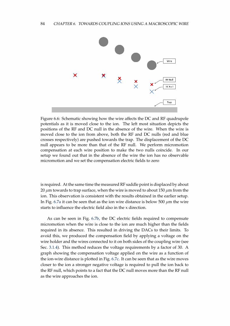
84 CHAPTER 6. TOWARDS COUPLING IONS USING A MACROSCOPIC WIRE
Figure 6.6: Schematic showing how the wire affects the DC and RF quadrupolepotentials as it is moved close to the ion. The left most situation depicts thepositions of the RF and DC null in the absence of the wire. When the wire ismoved close to the ion from above, both the RF and DC nulls (red and bluecrosses respectively) are pushed towards the trap. The displacement of the DCnull appears to be more than that of the RF null. We perform micromotioncompensation at each wire position to make the two nulls coincide. In oursetup we found out that in the absence of the wire the ion has no observablemicromotion and we set the compensation electric fields to zero
is required. At the same time the measured RF saddle point is displaced by about20 µm towards to trap surface, when the wire is moved to about 150 µm from theion. This observation is consistent with the results obtained in the earlier setup.In Fig. 6.7a it can be seen that as the ion wire distance is below 500 µm the wirestarts to influence the electric field also in the x direction.
As can be seen in Fig. 6.7b, the DC electric fields required to compensatemicromotion when the wire is close to the ion are much higher than the fieldsrequired in its absence. This resulted in driving the DACs to their limits. Toavoid this, we produced the compensation field by applying a voltage on thewire holder and the wires connected to it on both sides of the coupling wire (seeSec. 3.1.4). This method reduces the voltage requirements by a factor of 30. Agraph showing the compensation voltage applied on the wire as a function ofthe ion-wire distance is plotted in Fig. 6.7c. It can be seen that as the wire movescloser to the ion a stronger negative voltage is required to pull the ion back tothe RF null, which points to a fact that the DC null moves more than the RF nullas the wire approaches the ion.
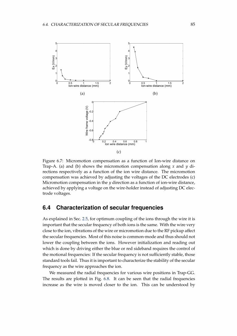
6.4. CHARACTERIZATION OF SECULAR FREQUENCIES 85
0 0.5 1 1.5 20
1
2
3
4
5
Ion-wire distance (mm)
Ex
(V/m
m)
(a)
0 0.5 1 1.5 20
1
2
3
4
5
Ion-wire distance (mm)
Ey
(V/m
m)
(b)
0 0.2 0.4 0.6 0.8 1-0.8
-0.6
-0.4
-0.2
0
Ion wire distance (mm)
Wire
fra
me
volta
ge
(V)
(c)
Figure 6.7: Micromotion compensation as a function of Ion-wire distance onTrap-A. (a) and (b) shows the micromotion compensation along x and y di-rections respectively as a function of the ion wire distance. The micromotioncompensation was achieved by adjusting the voltages of the DC electrodes (c)Micromotion compensation in the y direction as a function of ion-wire distance,achieved by applying a voltage on the wire-holder instead of adjusting DC elec-trode voltages.
6.4 Characterization of secular frequencies
As explained in Sec. 2.5, for optimum coupling of the ions through the wire it isimportant that the secular frequency of both ions is the same. With the wire veryclose to the ion, vibrations of the wire or micromotion due to the RF pickup affectthe secular frequencies. Most of this noise is common-mode and thus should notlower the coupling between the ions. However initialization and reading outwhich is done by driving either the blue or red sideband requires the control ofthe motional frequencies: If the secular frequency is not sufficiently stable, thosestandard tools fail. Thus it is important to characterize the stability of the secularfrequency as the wire approaches the ion.
We measured the radial frequencies for various wire positions in Trap-GG.The results are plotted in Fig. 6.8. It can be seen that the radial frequenciesincrease as the wire is moved closer to the ion. This can be understood by

86 CHAPTER 6. TOWARDS COUPLING IONS USING A MACROSCOPIC WIRE
0 1 2 3 4 50
0.5
1
1.5
2
2.5
Ion-wire distance (mm)
Fre
quency(M
Hz)
ωy
ωx
Figure 6.8: Plot showing the change in the radial secular frequencies of the ionas a function of the ion-wire distance. As the wire moves closer it appearsthat the curvature of the RF field increases resulting in an increase of the radialfrequencies along the radial directions.
realizing that the wire acts as an additional ground electrode. This argument isverified through an electrostatic modeling of the trap with a grounded wire.
6.5 Characterization of Heating rates
As is discussed in Sec. 2.5.2, heating in the ion traps is probably by far themost prominent source of decoherence in this experiment. We already pointedout that dust particles on the surfaces close to the ion are some of the majorcontributors for motional heating. With the electrically floating wire at a distancecloser than the ion-electrode distance these effects can intensify. These reasonsmake the characterization of the heating rate in the presence of wire an importantprerequisite for the wire-coupling experiment. In this section we present heatingrate measurements performed at different ion-wire distances. The measurementswere carried out in Trap-A with the wire assembly described in Sec. 3.1.4. Foreach wire position micromotion compensation was achieved using the RF drivestrength method (see Sec. 4.1.2).
The axial mode heating rates were measured using the sideband comparisonmethod described in Sec. 2.4.1 and the results are shown in Fig. 6.9a. Themeasurements were performed with an axial secular frequency ofωz = 2π·1 MHzup to an ion-wire distance of 120 µm. The heating of the axial mode increased

6.5. CHARACTERIZATION OF HEATING RATES 87
rapidly as the wire is moved close to the ion. The least square analysis of thedata with a 1/xn function yielded n = 1.96. So far reasons for this rapid increasein the heating rate of the axial mode is not clear.
Figure 6.9b shows the heating rate of the radial x mode as a function ofthe ion-wire distance. At small ion-wire distances the instability of the radialmotional modes prevented us from measuring the heating rates at ion-wiredistances below 180 µm. Unlike the axial, z mode, the x mode does not show anydramatic increase in the heating as the wire is moved close to the ion. Becausethe length of the wire is much bigger than the offset of the ion from the axis ofthe wire (see Fig. 6.4), the projection of the electric field noise of the wire on the zmode is large compared to the x mode. This might be one of the reasons for theobserved difference in the heating rates between the z and x modes.
Because of the small projection of the laser beam on the vertical y mode(discussed in detail in Sec. 4) the sideband cooling and the heating rate measure-ments could not be performed on it. However we have devised a new techniqueto transfer the motional energy between the modes, which can be used for thesideband cooling and the motional state measurement of the y mode. The detailsof this method are published in [81] and will be summarized in different thesisin the future.

88 CHAPTER 6. TOWARDS COUPLING IONS USING A MACROSCOPIC WIRE
0 500 1000 1500 20000
1
2
3
4
5
6
7
8
9
10
Ion-wire distance (m)
He
atin
g ra
te (
100
0 qu
anta
/s)
102
103
103
104
Ion-wire distance (m)
He
atin
g r
ate
(q
uan
ta/s
)
(a)
0 200 400 600 800 1000 1200 1400 16000
0.1
0.2
0.3
0.4
0.5
0.6
0.7
Ion-wire distance (m)
He
atin
g ra
te (
100
0 qu
anta
/s)
(b)
Figure 6.9: Plot showing the heating rate as a function of the ion-wire distance.The measurements were performed using the sideband comparison methoddescribed in Sec. 2.4.1. a) Plot showing the heating rate of the axial mode. Thedotted line is a 1/xn fit of the data with n = 1.96. The inset shows the sameaxial mode heating rate date plotted in logarithmic scale. The curve saturates athigher ion-wire distances because of the non-zero values of the heating rates inthe absence of the wire. b) Plot showing the heating rate of the radial x modefitted with a linear function. The heating rate of this mode does not show anyvisible increase up to an ion-wire distance of 180 µm.

Chapter 7
Summary
The main goal of this thesis was to prepare methods for experiments to coupletwo independently trapped ions using a metallic wire. The theoretical analysissuggest that quantum information can be transferred from one ion to anotherthrough the wire without much loss, even at room temperature. This approachwill not only ease scalability of ion trap quantum computing, but also can beused to construct hybrid quantum computing devices by connecting an ion trapto solid state devices such as superconducting qubits.
In this thesis, we have described our attempts to solve some of the keyproblems of the surface trap by gaining a better understanding of some of theimportant issues like stray charges and electric field noise on surface traps. Thediscussed techniques will be essential to perform any meaningful and complexexperiments with surface traps. We also present techniques helping us to coupletwo ions using a macroscopic metallic wire.
The multipole expansion method presented in this thesis to control the DCpotential is an useful tool for the experiments working with segmented ion traps.This method allowed us to adjust a particular trap parameter independentlywithout affecting the rest of the parameters. This is an efficient method, especiallyin the experiments like ours, where we need to control independently trappedions on the same trap chip.
The vacuum chamber setup discussed in this thesis is efficient in achievingthe ultra high vacuum necessary for the experiments. But in the future setupsthe placement of the ion pump must be chosen carefully to prevent the highmagnetic fields we experience in our setup. Utmost care has to be taken tokeep the trap clean because any dust particle close to the ion position results insevere stray electric fields and motional heating of the ion. The photoionizationlaser beams are overlapped only at the trap position to reduce the number ofphotoelectrons created.
89

90 CHAPTER 7. SUMMARY
In this thesis, we present a micromotion compensation method well suited forplanar ion traps. This technique relies on detecting the micromotion by drivingthe motional frequency of the ion if it is displaced from the RF null. This methodis fairly simple and does not require ultra stable lasers for the detection. We alsopresent heating rate measurements to understand the sources of the electric fieldfluctuations. It appears that the sources of both the field fluctuations and thestray charges are related.
First attempts of the ion-wire interactions showed that the wire can be movedto a distance of 80 µm from the ion. The compensation voltages were measuredas a function of ion-wire distance and they were found to be reproducible to agood extent for multiple wire approaches. The axial secular mode of the ionswas heating up fast, as the wire approached the ion, but the horizontal radialmode remained at the same temperature. The effect of the ion-wire distance onthe temperature of the vertical radial mode, which is more interesting, remainsto be examined.
7.1 Outlook
The future directions of the work presented in this thesis can be divided into thefollowing categories.
Hardware
In the current setup the wire is mounted on a separate holder and it is positionednear the ion using piezo driven nano-positioning stages. In this approach com-plications like the intermittent behavior of piezo stages and the failure of thewire resulted in significant setbacks in the progress of the experiment. To over-come these issues, we are planning to incorporate the floating wire into the trap.Efforts are being made to optimize the capacitance of such a wire configurationto the trap electrodes, to reduce the leakage of the coupling signal
Experiment
The first step towards coupling the two independently trapped ions using thewire is to trap an ion cloud in one of the wells and a single ion in the second welland examine if the current induced by the cloud in the wire can be detected withthe single ion in the second well through the wire. The vision of this experiment,however, is to test whether quantum information survives the passage throughthe wire between two independently trapped ions.

Bibliography
[1] R. Feynman. Simulating physics with computers. Int. J. Theoret. Phys., 21:467, 1982.[cited at p. 1]
[2] Yu. Manin. Computable and uncomputable. Sovetskoye Radio, Moscow, 1980.[cited at p. 1]
[3] P. W. Shor. Algorithms for quantum computation: discrete logarithms and factor-ing. In Proceedings of the 35th Annual Symposium on Foundations of Computer Science,Santa Fe, NM, Nov. 20-22, IEEE. Computer Society Press, pp. 124–134, 1994. [cited at p. 1]
[4] P. W. Shor. Scheme for reducing decoherence in quantum computer memory.Physical review A., 52(4):2493–2496, October 1995. [cited at p. 1]
[5] L. K. Grover. A. fast quantum mechanical algorithm for database search. Proceedingof the 28th ACM. STOC., page 212, 1996. [cited at p. 1]
[6] J. I. Cirac and P. Zoller. Quantum Computations with Cold Trapped Ions. Phys.Rev. Lett., 74(20):4091–4094, May 1995. [cited at p. 1, 25]
[7] Toschek P. E. Neuhauser W., Hohenstatt M. and Dehmelt H. Localized visible ba+
mono-ion oscillator. Phys. Rev., A22:11371140, 1980. [cited at p. 1]
[8] W. Neuhauser, M. Hohenstatt, P. Toschek, and H. Dehmelt. Optical-SidebandCooling of Visible Atom Cloud Confined in Parabolic Well. Phys. Rev. Lett., 41:233,1978. [cited at p. 1, 19]
[9] Q. A. Turchette, C. S. Wood, B. E. King, C. J. Myatt, D. Leibfried, W. M. Itano, C. Mon-roe, and D. J. Wineland. Deterministic entanglement of two ions. Phys.˜Rev.˜Lett.,81:3631, 1998. [cited at p. 1, 8]
[10] C. A. Sackett, D. Kielpinski, B. E. King, C. Langer, V. Meyer, C. J. Myatt, M. Rowe,Q. A. Turchette, W. M. Itano, D. J. Wineland, and C. Monroe. Experimental entan-glement of four particles. Nature, 404:256–259, 2000. [cited at p. 1, 8]
[11] B. DeMarco, A. Ben-Kish, D. Leibfried, V. Meyer, M. Rowe, B. M. Jelenkovic, W. M.Itano, J. Britton, C. Langer, T. Rosenband, and Others. Experimental demonstrationof a controlled-NOT wave-packet gate. Physical review letters, 89(26):267901, 2002.[cited at p. 1, 8]
91

92 BIBLIOGRAPHY
[12] Stephan Gulde, Mark Riebe, Gavin P. T. Lancaster, Christoph Becher, Jurgen Es-chner, Hartmut Haffner, Ferdinand Schmidt-Kaler, Isaac L. Chuang, and RainerBlatt. Implementation of the Deutsch-Jozsa algorithm on an ion-trap quantumcomputer. Nature, 421(6918):48–50, 2003. [cited at p. 1, 8]
[13] M. D. Barrett, J. Chiaverini, T. Schaetz, J. Britton, W. M. Itano, J. D. Jost, E. Knill,C. Langer, D. Leibfried, R. Ozeri, and D. J. Wineland. Deterministic quantumteleportation of atomic qubits. Nature, 429:737–739, 2004. [cited at p. 1, 8]
[14] H. Haffner, W. Hansel, C. F. Roos, J. Benhelm, D. Chek-al Kar, M. Chwalla, T. Korber,U. D. Rapol, M. Riebe, P. O. Schmidt, C. Becher, O. Guhne, W. Dur, and R. Blatt.Scalable multiparticle entanglement of trapped ions. Nature, 438:643–646, 2005.[cited at p. 1, 8]
[15] P. J. Lee, K. A. Brickman, L. Deslauriers, P. C. Haljan, L. M. Duan, and C. Monroe.Phase control of trapped ion quantum gates. J.˜Opt.˜B, 7:371, 2005. [cited at p. 1, 8]
[16] J. Benhelm, G. Kirchmair, C. F. Roos, and R. Blatt. Towards fault-tolerant quantumcomputing with trapped ions. Nature Physics, 4:463, 2008. [cited at p. 1, 8]
[17] G. Kirchmair, F. Zahringer, R. Gerritsma, M. Kleinmann, O. Guhne, a. Cabello,R. Blatt, and C. F. Roos. State-independent experimental test of quantum contextu-ality. Nature, 460(7254):494–497, July 2009. [cited at p. 1]
[18] R. J. Hughes, D. F. V. James, E. H. Knill, R. Laflamme, and A. G. Petschek. De-coherence Bounds on Quantum Computation with Trapped Ions. Phys.˜Rev.˜Lett.,77:3240–3243, 1996. [cited at p. 2]
[19] D. J. Wineland, C. Monroe, W. M. Itano, D. Leibfried, B. E. King, and D. M. Meekhof.Experimental Issues in Coherent Quantum-State Manipulation of Trapped AtomicIons. Journal of Research of the National Institute for Standards and Technology, 103:259–328, 1998. [cited at p. 2, 30, 49, 67]
[20] D. Kielpinski, C. Monroe, and D. J. Wineland. Architecture for a large-scale ion-trapquantum computer. Nature, 417(6890):709–711, 2002. [cited at p. 2, 8, 67]
[21] J. Chiaverini, R. B. Blakestad, J. Britton, J. D. Jost, C. Langer, D. Leibfried, R. Ozeri,and D. J. Wineland. Surface-electrode architecture for ion-trap quantum informa-tion processing. Quantum Information and Computation, 5:419–439, 2005. [cited at p. 2,
8, 9]
[22] S. Seidelin, J. Chiaverini, R. Reichle, J. J. Bollinger, D. Leibfried, J. Britton, J. H. We-senberg, R. B. Blakestad, R. J. Epstein, D. B. Hume, W. M. Itano, J. D. Jost, C. Langer,R. Ozeri, N. Shiga, and D. J. Wineland. Microfabricated surface-electrode ion trapfor scalable quantum information processing. Physical Review Letters, 96:253003,2006. [cited at p. 2, 8]
[23] J. Britton, D. Leibfried, J. Beall, R. B. Blakestad, J. J. Bollinger, J. Chiaverini, R. J.Epstein, J. D. Jost, D. Kielpinski, C. Langer, R. Ozeri, R. Reichle, S. Seidelin, N. Shiga,J. H. Wesenberg, and D. J. Wineland. A. microfabricated surface-electrode ion trapin silicon. arXiv:quant-ph/0605170v1, 2008. [cited at p. 2]

BIBLIOGRAPHY 93
[24] C. Monroe, D. M. Meekhof, B. E. King, W. M. Itano, and D. J. Wineland. Demon-stration of a fundamental quantum logic gate. Phys. Rev. Lett., 75:4714–4717, 1995.[cited at p. 2, 67]
[25] S. Narayanan, N. Daniilidis, S. Moller, R. Clark, F. Ziesel, K. Singer, F. Schmidt-Kaler, and H. Haffner. Electric field compensation and sensing with a single ion ina planar trap. Journal of Applied Physics, 110(11):114909, 2011. [cited at p. 3, 51]
[26] J. D. Jackson. Classical Electrodynamics. John Wiley & Sons, New York, 3rd edition,1998. [cited at p. 5, 9, 26, 27]
[27] W. Paul and H. Steinwedel. Ein neues Massenspektrometer ohne Magnetfeld.Naturforschung, A. 8:448450, 1953. [cited at p. 5]
[28] O. Osberghaus W. Paul and E. Fischer. Ein Ionenkafig. Forschungsberichte desWirtschafts und Verkehrsministerium Nordrhein-Westfalen, page 415, 1958. [cited at p. 5]
[29] Wolfgang Paul. Electromagnetic traps for charged and neutral particles. Reviews ofModern Physics, 62(3):531–540, July 1990. [cited at p. 6]
[30] D. Leibfried, R. Blatt, C. Monroe, and D. Wineland. Quantum dynamics of singletrapped ions. Reviews of Modern Physics, 75(1):281–324, March 2003. [cited at p. 7, 14,
16, 19, 20, 21, 22, 30]
[31] Gebhard Littich. Electrostatic Control and Transport of Ions on a Planar Trap for QuantumInformation Processing. Master thesis, ETH. Zurich and University of California,Berkeley, 2011. [cited at p. 9, 78]
[32] Christian Felix Roos. Controlling the quantum state of trapped ions. Doctoral thesis,University of Innsbruck, 2000. [cited at p. 14]
[33] H. G. Dehmelt. Radiofrequency Spectroscopy of Stored Ions I: Storage. Adv. At.Mol. Phys, 3:53–72, 1967. [cited at p. 14]
[34] E. T. Jaynes and F. W. Cummings. Comparison of quantum and semiclassicalradiation theories with application to the beam maser. Proceedings of the IEEE.,14:89, 1963. [cited at p. 16]
[35] I. Marzoli, J. I. Cirac, R. Blatt, and P. Zoller. Laser cooling of trapped three-levelions: Designing two-level systems for sideband cooling. Phys.˜Rev.˜A, 49:2771–2779,1994. [cited at p. 19]
[36] D. J. Wineland, R. E. Drullinger, and F. L. Walls. Radiation-pressure cooling ofbound resonant absorbers. Phys. Rev. Lett., 40:1639, 1978. [cited at p. 19]
[37] Peter Van der Straten Harold J. Metcalf. Laser cooling and trapping. Spinger, NewYork, 1999. [cited at p. 19]
[38] J. I. Cirac, L. J. Garay, R. Blatt, A. S. Parkins, and P. Zoller. Laser cooling of trappedions: The influence of micromotion. Phys. Rev. A, 49:421–432, 1994. [cited at p. 19]
[39] P. K. Ghosh. Ion traps. Clarendon Press, Oxford, 1st edition, 1996. [cited at p. 20]

94 BIBLIOGRAPHY
[40] F. Diedrich, J. C. Bergquist, Wayne M. Itano, and D. J. Wineland. Laser Coolingto the Zero-Point Energy of Motion. Physical Review Letters, 62(4):403–406, January1989. [cited at p. 20, 23]
[41] Ch. Roos, Th. Zeiger, H. Rohde, H. C. Nagerl, J. Eschner, D. Leibfried, F. Schmidt-Kaler, and R. Blatt. Quantum state engineering on an optical transition and deco-herence in a Paul trap. Physical Review Letters, 83:4713, 1999. [cited at p. 20]
[42] J. H. Wesenberg, R. J. Epstein, D. Leibfried, R. B. Blakestad, J. Britton, J. P. Home,W. M. Itano, J. D. Jost, E. Knill, and C. Langer. Fluorescence during Doppler coolingof a single trapped atom. Physical Review A., 76(5):53416, 2007. [cited at p. 24, 50, 54, 71,
72, 73]
[43] D. Kielpinski, V. Meyer, M. A. Rowe, C. A. Sackett, W. M. Itano, C. Monroe, andD. J. Wineland. A. decoherence-free quantum memory using trapped ions. Science,291(5506):1013–1015, February 2001. [cited at p. 24]
[44] I. Cirac, P. Zoller, J. Kimble, and H. Mabuchi. Quantum State Transfer and En-tanglement Distribution among Distant Nodes in a Quantum Network. Phys. Rev.Lett., 78:3221, 1997. [cited at p. 24]
[45] H. J. Kimble. The quantum internet. Nature, 453(7198):1023–1030, June 2008.[cited at p. 24]
[46] D. L. Moehring, P. Maunz, S. Olmschenk, K. C. Younge, D. N. Matsukevich, L-M.Duan, and C. Monroe. Entanglement of single-atom quantum bits at a distance.Nature, 449(7158):68–71, 2007. [cited at p. 24]
[47] D. Gottesman and I. L. Chuang. Quantum teleportation is a universal computa-tional primitive. Nature, 402:390, 1999. [cited at p. 24]
[48] D. J. Wineland and H. G. Dehmelt. Principles of the stored ion calorimeter. J. App.Phys., 46:919, 1975. [cited at p. 24, 26]
[49] D. J. Heinzen and D. J. Wineland. Quantum-limited Cooling and Detection ofRadio-Frequency Oscillations by Laser-cooled Ions. Phys. Rev. A., 42:2977, 1990.[cited at p. 24, 26]
[50] Sørensen, A. S., Wal, C. H. V. D., Childress, L. I. and Lukin, M. D. Capacitive Cou-pling of Atomic Systems to Mesoscopic Conductors. Phys. Rev. Lett., 92(6):063601,2004. [cited at p. 24]
[51] S. Stahl, F. Galve, J. Alonso, S. Djekic, W. Quint, T. Valenzuela, J. Verdu, M. Vogel,G. Werth, and J. Verd. A. planar Penning trap. The European Physical Journal D.,32(1):139–146, December 2004. [cited at p. 24]
[52] Melba Phillips Wolfgang K. H. Panofsky. Classical Electricity and Magnetism.Addison-Wesley Pub. Co., 2nd edition, 1962. [cited at p. 26]
[53] Lee E. Estes, Thomas H. Keil, and Lorenzo M. Narducci. Quantum-MechanicalDescription of Two Coupled Harmonic Oscillators. Phys. Rev., 175(1):286–299,November 1968. [cited at p. 27, 99]

BIBLIOGRAPHY 95
[54] Rodrigues H. Duarte S. B., Portes D and Baseia B. Quantum states transfer betweencoupled fields. Eur. Phys.J., D48:145149, 2008. [cited at p. 28]
[55] Jorge R. Zurita-Sanchez and Carsten Henkel. Wiring up single electron traps to per-form quantum gates. New Journal of Physics, 10(8):083021, August 2008. [cited at p. 29]
[56] Q. A. Turchette, Kielpinski, B. E. King, D. Leibfried, D. M. Meekhof, C. J. My-att, M. A. Rowe, C. A. Sackett, C. S. Wood, W. M. Itano, C. Monroe, and D. J.Wineland. Heating of trapped ions from the quantum ground state. Physical Re-view A., 61:63418, 2000. [cited at p. 30, 54, 67, 74]
[57] N. Daniilidis, S. Gerber, G. Bolloten, M. Ramm, A. Ransford, E. Ulin-Avila, I. Taluk-dar, and H. Haffner. Surface noise analysis using a single-ion sensor. Physical ReviewB., 89(24):245435, June 2014. [cited at p. 30]
[58] J. Labaziewicz, Y. Ge, P. Antohi, D. Leibrandt, K. R. Brown, and I. L. Chuang.Suppression of Heating Rates in Cryogenic Surface-Electrode Ion Traps. PhysicalReview Letters, 100:13001, 2008. [cited at p. 30]
[59] Jaroslaw Labaziewicz, Yufei Ge, David Leibrandt, Shannon X. Wang, Ruth Shew-mon, and Isaac L. Chuang. Temperature Dependence of Electric Field Noise AboveGold Surfaces. Physical Review Letters, 101:180602, 2008. [cited at p. 30]
[60] P. Schindler, D.J. Gorman, N. Daniilidis, H. Hffner. Polarization of electric-fieldnoise near metallic surfaces. Phys. Rev. A, 92:013414, 2015. [cited at p. 32]
[61] N. Daniilidis, S. Narayanan, S. Moller, R. Clark, T. Lee, P. Leek, A. Wallraff, St Schulz,F. Schmidt-Kaler, and H. Haffner. Fabrication and heating-rate study of microscopicsurface electrode traps. New J. Phys., 13:013032, 2011. [cited at p. 32]
[62] M. Block, P. Seibert, O. Rehm, and G. Werth. 3D5/2 lifetime in laser cooled Ca+:Influence of cooling laser power. Eur. Phys.J., D7(3):461, 1999. [cited at p. 39]
[63] E. Rabinowicz. Friction and Wear of Materials. John Wiley & Sons, New York, 1965.[cited at p. 42, 80]
[64] W.W. Macalpine, and R.O. Schildknecht. Coaxial resonators with helical innerconductor. Proc. IRE, 47:2099, 1959. [cited at p. 44]
[65] J.D. Siverns, L.R. Simkins, S.Weidt and W.K. Hensinger. On the application of radiofrequency voltages to ion traps via helical resonators. Appl Phys B, 107:921–934,2012. [cited at p. 44]
[66] Michael Ramm. Quantum Correlations and Energy Transport in Trapped Ions. Doctoralthesis, University of California, Berkeley, 2014. [cited at p. 46]
[67] Thaned Pruttivarasin. Spectroscopy, fundamental symmetry tests and quantum simu-lation with trapped ions. Doctoral thesis, University of California, Berkeley, 2014.[cited at p. 46]
[68] DJ. Berkeland, JD. Miller, JC. Bergquist, WM. Itano, and DJ Wineland. Minimizationof ion micromotion in a Paul trap. Journal of Applied Physics, 83(10):5025, 1998.[cited at p. 49]
96 BIBLIOGRAPHY
[69] D. T. C. Allcock, J. A. Sherman, D. N. Stacey, A. H. Burrell, M. J. Curtis, G. Imreh,N. M. Linke, D. J. Szwer, S. C. Webster, A. M. Steane, and D. M. Lucas. Implemen-tation of a symmetric surface-electrode ion trap with field compensation using amodulated Raman effect. New Journal of Physics, 12(5):053026, May 2010. [cited at p. 50]
[70] Stephan A. Schulz, Ulrich Poschinger, Frank Ziesel, Ferdinand Schmidt-Kaler, andSchmidt-Kaler F. Schulz S, Poschinger U, Ziesel F. Sideband cooling and coherentdynamics in a microchip multi-segmented ion trap. New J. Phys., 10(4):045007, April2008. [cited at p. 50]
[71] R. B. Blakestad, C. Ospelkaus, A. P. VanDevender, J. M. Amini, J. Britton,D. Leibfried, and D. J. Wineland. High-Fidelity Transport of Trapped-Ion Qubitsthrough an X-Junction Trap Array. Phys. Rev. Lett., 102(15):153002, April 2009.[cited at p. 50, 51, 52]
[72] Y. Ibaraki, U. Tanaka, and S. Urabe. Detection of parametric resonance of trappedions formicromotion compensation. Applied Physics B., 0(1):1–3, March 2011.[cited at p. 50, 51]
[73] T. Rosenband. Private communication. Technical report, 2009. [cited at p. 51]
[74] N. Akerman, S. Kotler, Y. Glickman, Y. Dallal, a. Keselman, and R. Ozeri. Single-ion nonlinear mechanical oscillator. Physical Review A., 82(6):3–6, December 2010.[cited at p. 51]
[75] B. Bosco and T. Sacchi, M. On the inversion problem in classical electrodynamicsand the ”Casimir theorem”. Annals of Physics, 12, 1981. [cited at p. 61]
[76] T. B. Smith. Best-fit multipole expansions for fields from static currents. InverseProblems, 1(2):173–179, May 1985. [cited at p. 61]
[77] D. T. C. Allcock, T. P. Harty, H. a. Janacek, N. M. Linke, C. J. Ballance, a. M.Steane, D. M. Lucas, R. L. Jarecki, S. D. Habermehl, M. G. Blain, D. Stick, and D. L.Moehring. Heating rate and electrode charging measurements in a scalable, micro-fabricated, surface-electrode ion trap. Applied Physics B., 107(4):913–919, November2011. [cited at p. 63]
[78] R. A. Millikan and Carl F. Eyring. Laws Governing the Pulling of Electrons out ofMetals by Intense Electrical Fields. Phys. Rev., 27:511, 1926. [cited at p. 63]
[79] R. A. Millikan and Carl F. Eyring. Relations of Field-Currents to Thermionic-Currents. Proceedings of the National Academy of Sciences of the United States of America,14:45–59, 1928. [cited at p. 63]
[80] R. J. Epstein, S. Seidelin, D. Leibfried, J. H. Wesenberg, J. J. Bollinger, J. M. Amini,R. B. Blakestad, J. Britton, J. P. Home, W. M. Itano, J. D. Jost, E. Knill, C. Langer,R. Ozeri, N. Shiga, and D. J. Wineland. Simplified motional heating rate measure-ments of trapped ions. Phys Rev A., 76:33411, 2007. [cited at p. 68]
[81] Dylan J. Gorman, Philipp Schindler, Sankaranarayanan Selvarajan, Nikos Dani-ilidis, and Hartmut Haffner. Two-mode coupling in a single-ion oscillator viaparametric resonance. Physical Review A., 89(6):062332, June 2014. [cited at p. 87]

BIBLIOGRAPHY 97
[82] D. Portes, H. Rodrigues, S. B. Duarte, and B. Baseia. Quantum states transferbetween coupled fields. The European Physical Journal D., 48(1):145–149, June 2008.[cited at p. 99, 100]


Appendix A
Quantum state transfer betweencoupled ions
In this section we study the time evolution of the above Hamiltonian for specificinitial states of the ions. A detail derivation of the time evolution is presentedin [53, 82].
The Hamiltonian for the coupled ion system in the presence of the floatingwire is
H =p2
1
2m+
12
mω21y2
1 +p2
2
2m+
12
mω22y2
2 + γy1y2. (A.1)
Where yi and pi are the position and momentum respectively of the ith ion. ωi
is the natural frequency of the ith ion along the y direction and γ is the couplingconstant between the ions. It was found that the rotating wave approximationis in almost complete agreement with the exact solution in the limit of smallcoupling constants (γ/mω2 < 0.1) [53].
In the resonant approximation the equation A.1 can be written as
H = ~ω(a†1a1 + 1/2) + ~ω(a†2a2 + 1/2) +~γ
2ω(a†1a2 + a†2a1). (A.2)
where a is referred as the annihilation operator given by
a =(mωx + ip
)( 12~mω
)1/2
. (A.3)
and a† is the Hermitian adjoint of a, referred as the creation operator.Let us consider the case where the first ion is in a coherent state |µ〉1, with
complex amplitude µ, and the second ion is in ground state |0〉2
99

100 APPENDIX A. QUANTUM STATE TRANSFER BETWEEN COUPLED IONS
|µ〉1 = e1/2|µ|2∞∑
n=0
µn
√n|n〉. (A.4)
The initial state of the system of ions |ψ(0)〉12 = |µ〉1 ⊗ |0〉2 can be denoted as
|ψ(0)〉 =
∞∑n=0
Cn,0(0)|n, 0〉. (A.5)
where Cn,0(0) is the probability amplitude of the system of ions for the state|n, 0〉 at time t = 0.
Assuming the resonance condition the probability amplitude of the systemfor the state |0,n〉 after a time t is given by [82]
C0,n(t) = Cn,0(0)e−i(ωt+π/2)n sinn(γt
2ωm
). (A.6)
The exchange of state will occur after an instance τ, when C0,n(τ) = Cn,0(0).However, in this case, with one of the ions initially in a coherent state, we donot obtain a perfect exchange of states due to the presence of the phase factorexp
[−i(ωτ+π/2)n
]affecting the coefficients of the state describing both oscillators
in the Focks representation.when t = tex = πωm/γ the above equation becomes
C0,n(tex) = Cn,0(0)e−iπ(ω2m/γ+1/2)n. (A.7)
which results in the first ion in the ground state and the second ion in acoherent state |µe−iΘ
〉, where Θ = π(ω2m/γ + 1/2) describes the change of thecoherent state’s complex amplitude. Here we obtain |C0,n(tex)| = |Cn,0(0)| whichmeans only exchange of statistics between subsystems.