ESTCPCost and Performance Report

ENVIRONMENTAL SECURITYTECHNOLOGY CERTIFICATION PROGRAM

U.S. Department of Defense

(UX-9812)

Electromagnetic Induction and Magnetic SensorFusion for Enhanced UXO Target Classification

February 2004

i

COST & PERFORMANCE REPORT ESTCP Project: UX-9812

TABLE OF CONTENTS

Page

1.0 EXECUTIVE SUMMARY ................................................................................................ 1 2.0 TECHNOLOGY DESCRIPTION ...................................................................................... 3 2.1 BACKGROUND AND INTENDED USE............................................................. 3 2.2 TECHNOLOGY DESCRIPTION .......................................................................... 3 2.2.1 Mobilization and Operational Requirements .............................................. 6

2.2.2 Personnel and Training Requirements ........................................................ 7 2.2.3 Health and Safety Training ......................................................................... 8 2.3 ADVANTAGES AND LIMITATIONS OF THE TECHNOLOGY...................... 8 3.0 DEMONSTRATION DESIGN .......................................................................................... 9 3.1 PERFORMANCE OBJECTIVES .......................................................................... 9 3.1.1 L Range Demonstration .............................................................................. 9 3.1.2 BBR Impact Area Demonstration............................................................... 9 3.2 SELECTION OF TEST SITES ............................................................................ 10 3.3 TEST SITE HISTORY AND CHARACTERISTICS .......................................... 11 3.3.1 L Range Demonstration ............................................................................ 11 3.3.2 BBR Impact Area Demonstration............................................................. 12 3.4 PHYSICAL SETUP AND OPERATION ............................................................ 14 3.4.1 L Range Demonstration ............................................................................ 14 3.4.2 BBR Impact Area Demonstration............................................................. 14 4.0 PERFORMANCE ASSESSMENT .................................................................................. 17 4.1 L RANGE DEMONSTRATION.......................................................................... 17 4.1.1 Remediation Results ................................................................................. 17 4.1.2 Performance Data...................................................................................... 18 4.1.3 Data Assessment ....................................................................................... 20 4.1.4 Technology Comparison........................................................................... 21 4.2 BBR IMPACT AREA SURVEY.......................................................................... 23 4.2.1 Pre-Demonstration Measurements............................................................ 23 4.2.2 Survey Data............................................................................................... 26 4.2.3 Data Assessment ....................................................................................... 27 4.2.3.1 EM61 MkII Electronic and Calibration Issues .............................27 4.2.3.2 EM61 MkI Signal to Noise Ratios................................................29 4.2.3.3 EM61 Model Fits ..........................................................................31 4.2.3.4 An Alternate Discrimination Approach ........................................33 4.2.3.5 Technology Comparison...............................................................36

ii

TABLE OF CONTENTS (continued)

Page 5.0 COST ASSESSMENT...................................................................................................... 39 5.1 COST ANALYSIS................................................................................................ 39 5.2 COST COMPARISON ......................................................................................... 40 6.0 REFERENCES ................................................................................................................. 41 APPENDIX A POINTS OF CONTACT............................................................................ A-1 APPENDIX B MTADS TARGET REPORT FROM THE L RANGE DEMONSTRATION ..................................................................................B-1 APPENDIX C MTADS TARGET REPORT FROM THE BBR IMPACT AREA DEMONOSTRATION ...................................................................C-1

iii

FIGURES

Page Figure 1. Direction and Magnitude of the Magnetic Field Transmitted by the MTADS EM61 Array ..............................................................................................5 Figure 2. Road Map Showing Location of the L Range. ......................................................11 Figure 3. Aerial View of the Army Research Laboratory Blossom Point L Range with Approximate Location of the First Demonstration Highlighted....................12 Figure 4. A Portion of USGS 7.5-Minute Map with the Perimeter of the BBR Impact Area Shown in Red ...........................................................................13 Figure 5. Aerial Photograph of Logistics Support for the Second Demonstration ...............15 Figure 6. Example 81-mm Mortar and 60-mm Mortar Remediated at the L Range.............17 Figure 7. Example of Nonordnance Remediated at L Range................................................17 Figure 8. Two-Dimensional Representation of the Three-Beta Fits for 81-mm Mortars in the Demonstration ................................................................................18 Figure 9. Two-Dimensional Representation of the Three-Beta Fits for Other Recovered Targets from the Demonstration Plotted as in Figure 8.......................19 Figure 10. ROC Curve for the Detection of 81-mm Mortars..................................................19 Figure 11. ROC Curve for the Detection of All Ordnance .....................................................19 Figure 12. Two-Dimensional Representation of Three Beta Fits for All Targets Dug in the Demonstration with Ellipses for Each Ordnance Class Derived from the 81-mm Mortar Ellipse......................................................................................20 Figure 13. Results of a Monte Carlo Simulation of Fitted Betas Resulting from a Range of Model 81-mm Mortars with Two Sources of Noise Compared to the Results from the First Demonstration ....................................................................22 Figure 14. ROC Curve for Classification Using These Methods Compared to Results Using Magnetic Dipole Size and Dipole Orientation ...............................23 Figure 15. Measured EM63 Response Profiles at Eight Time Gates from a Traverse over a Horizontal 105-mm Projectile 66 cm below the Sensor .............................24 Figure 16. Measured EM63 Response Profiles at Eight Time Gates from a Traverse over a Frag Cluster.................................................................................................25 Figure 17. Comparison of the Results of All Three Surveys of the Seeded Area in a Small Subgrid.........................................................................................................26 Figure 18. Comparison of the Signals from the EM61 MkII Array and the EM61 MkI Array Arising from a High-SNR 105-mm Projectile..........................28 Figure 19. Comparison of the Signals from the EM61 MkII Array and the EM61 MkI Array Arising from a Low-SNR105-mm Projectile ...........................29 Figure 20. Comparison of the Noise Observed with the EM61 MkI at Three Sites ...............30 Figure 21. Power Spectral Density of the EM61 MkI Noise at Two Sites .............................30 Figure 22. Plots of Primary Beta Versus Secondary Beta for Ordnance Items and Clutter....31 Figure 23. Data Fit and Chi-Square Contours for a High-SNR 155-mm Projectile ...............32 Figure 24. Data Fit and Chi-Square Contours for a Low-SNR 155-mm Projectile ................32 Figure 25. Data Fit and Chi-Square Contours for a Frag Cluster............................................33 Figure 26. Plots of Reduced Chi-Square Versus Peak Signal for Ordnance and Clutter........34 Figure 27. Comparison of Beta Sphere Discriminant to Goodness-of-Fit Discriminant. .......35

iv

FIGURES (continued)

Page Figure 28. Results of the Constrained Fits ..............................................................................35 Figure 29. ROC Curves Comparing the Discrimination Performance of the Three Methods..................................................................................................................36 Figure 30. ROC Curves Comparing the Discrimination Performance of the Constrained Beta Fit with the Two Magnetometry Analyses Used in this Demonstration .......37

TABLES

Page Table 1. Typical Logistics Costs for a 2-Week Survey Assuming No Remediation.............7 Table 2. Impact Area Survey Coordinates Provided by Ellsworth AFB .............................14 Table 3. Schedule for the L Range Demonstration..............................................................14 Table 4. Location of Emplaced Seed Targets at the BBR Impact Area...............................15 Table 5. Schedule for the BBR Impact Area Demonstration...............................................16 Table 6. Size Distributions Used in Magnetometer Analysis of the Demonstration Results ...........................................................................................22 Table 7. Gate Times for the Two Modes of the MTADS EM61 MkIIs ..............................25 Table 8. Summary of the Magnetometer Analysis Results..................................................26 Table 9. Cost Comparison for a Hypothetical 200-Acre Survey Using These Methods .....39

v

ACRONYMS AND ABBREVIATIONS

AFB Air Force Base APG Aberdeen Proving Ground ARL Army Research Laboratory ATC Aberdeen Test Center BBR Badlands Bombing Range, SD CES Civil Engineer Squadron DAS data analysis system DoD Department of Defense EM electromagnetic EOD explosives ordnance disposal ERDC Engineer Research and Development Center ESTCP Environmental Security Technology Certification Program FA false alarm GIS geographic information system GPS global positioning system HAZWOPR hazardous waste operations IDA Institute for Defense Analyses JPG Jefferson Proving Ground ms milliseconds MTADS Multi-Sensor Towed Array Detection System NBS National Bureau of Standards NIST National Institute of Standards and Technology NRL Naval Research Laboratory OST Oglala Sioux Tribe PD probability of detection PNN probabilistic neural net QC quality control

ACRONYMS AND ABBREVIATIONS (continued)

vi

RMS root mean square ROC receiver operating characteristic RTK real-time kinematic SERDP Strategic Environmental Research and Development Program SNR signal to noise ratio S/N signal to noise USGS U.S. Geological Survey UXO Unexploded Ordnance

vii

ACKNOWLEDGEMENTS

The Multi-Sensor Towed Array Detection System (MTADS) development and initial demonstrations were supported by the Environmental Security Technology Certification Program (ESTCP) Program Office. This program, aimed to increase the classification ability of the MTADS system, was also supported by ESTCP. The Naval Research Laboratory has managed all MTADS activities. The principal investigator for this program is Dr. H.H. Nelson. Dr. J. R. McDonald is the deputy principal investigator. We wish to acknowledge the critically important contributions made by AETC, Inc. Tom Bell, Bruce Barrow, and Nagi Khadr were instrumental in the development of the model used in this program, and Bernard Puc modified the data analysis system to make use of these methods. We appreciate continual program administrative support by Richard Robertson (Hughes Associates) and field support by Larry Koppe (GeoCenters, Inc.) and Glenn Harbaugh (Nova Research, Inc.). Finally, we wish to express our grateful appreciation to Dr. Jeff Marqusee for his unflagging and continual commitment to developing and refining automated UXO detection and remediation technologies. This commitment has led to demonstration and validation of a fully field-hardened prototype and to its transition to the commercial sector where it is currently available to provide commercial UXO services and continual improvements of our understanding and ability to make use of MTADS data.

Technical material contained in this report has been approved for public release.

This page left blank intentionally.

1

1.0 EXECUTIVE SUMMARY Traditional methods for buried unexploded ordnance (UXO) detection, characterization, and remediation are labor-intensive, slow, and inefficient. A large portion, approaching 70% in some cases, of the total budget of a typical remediation effort is spent on digging targets that do not turn out to be UXO. The Environmental Security Technology Certification Program (ESTCP), has supported the Naval Research Laboratory (NRL) in developing the Multi-Sensor Towed Array Detection System (MTADS), to address these deficiencies. It is efficient and simple to operate by relatively untrained personnel. It can detect and locate ordnance with accuracies on the order of 15 cm. However, even with careful mission planning and site-specific training, there are still significant numbers of nonordnance targets selected. Most UXO fit a specific profile: they are long and slender with typical length-to-diameter aspect ratios of four or five. Many clutter items, on the other hand, do not fit this profile. Using electromagnetic (EM) pulsed-induction sensor data, we have developed a model-based estimation procedure that relies on exploiting the dependence of the induced field on target size, shape, and orientation to determine if a target is likely to be a UXO item. These methods were the subject of two demonstrations. The first demonstration was conducted in August 1999 at a live test range, the L Range at the Army Research Laboratory’s (ARL) Blossom Point Facility. Towed-array magnetometer (one pass) and EM pulsed-induction data (two orthogonal passes) over the 3 acre site were collected in 12 survey hours. After analysis of the resulting data sets, 201 targets were classified by their EM response coefficients and flagged for remediation. Target remediation and identification required 12 man-days. Of the 188 targets recovered from this test area, 66 were ordnance items, 20 were ordnance-related items, 66 were exploded fragments, and 36 were items not related to ordnance. The ordnance items broke down into three groups: 48 81-mm mortars, 8 mortars of smaller sizes, and 10 miscellaneous ordnance items. The results of our analysis are presented graphically and receiver operating characteristic (ROC) curves are derived and compared to the baseline MTADS magnetometer analysis. For a single ordnance item, 81-mm mortars, we achieve roughly a 60% reduction in false alarms without impacting probability of detection (PD). In order to identify the small fuzes in this field as ordnance, a large number of clutter items have to be included as we are able to reject only ~25%. In part, this is the inevitable result of trying to discriminate ordnance ranging in size from fuzes to 5-in rockets from clutter. This difficulty may be mitigated by obtaining more data, hence better fit statistics, on the smaller ordnance items. The second demonstration was conducted in September 2001 at the Impact Area of the Badlands Bombing Range, South Dakota site that has been used as an artillery training area for many years. The demonstration was conducted on a portion of the site that had been cleared of ordnance in a previous MTADS demonstration. Twenty-five inert projectiles were seeded on the test area amid the existing clutter field. This was considered a good test of the discrimination

2

ability of the new analysis algorithms. Magnetometer and EM61 Mk I (single time gate as used in the first demonstration) and EM61 Mk II (four time gates) data were collected. The EM61 MkII (a relatively new sensor from Geonics, Limited) data proved to be of too low signal-to-noise ratio to be useful in classification. Using the EM61 MkI data, 70 anomalies exhibited signal amplitudes of at least twice the (relatively high) background. Several classification methodologies were employed on these anomalies, and the results are presented graphically. Compared to a traditional mag-and-flag survey, these methods cost 25% more per acre. Considering that mag-and-flag surveys detect only ~35% of deeper targets, these methods are far more cost effective on a detected target basis. The false alarm rejection mentioned above is not applicable to a mag-and-flag survey.

3

2.0 TECHNOLOGY DESCRIPTION 2.1 BACKGROUND AND INTENDED USE Buried UXO is one of the Department of Defense’s (DoD) most pressing environmental problems. Not limited to active ranges and bases, UXO contamination is also present at DoD sites that are dormant and in areas adjacent to military ranges that are under the control of other government agencies and the private sector. Traditional methods for buried UXO detection, characterization, and remediation are labor-intensive, slow, and inefficient. Typical detection and characterization methods rely on hand-held detectors operated by explosive ordnance disposal (EOD) technicians who walk slowly across the survey area. This process has been documented as inefficient and marginally effective.1 A large portion, approaching 70% in some cases, of the total budget of a typical remediation effort is spent on digging targets that do not turn out to be UXO. ESTCP has supported NRL in developing MTADS to address these deficiencies. MTADS incorporates both cesium vapor full-field magnetometers and EM pulsed-induction sensors in linear arrays that are towed over survey sites by an all-terrain vehicle. Sensor positioning is provided by state-of-the-art real-time kinematic (RTK) global positioning system (GPS) receivers. The survey data acquired by MTADS is analyzed by an NRL-developed data analysis system (DAS). DAS was designed to locate, identify, and categorize all military ordnance at its maximum self-burial depth. It is efficient and simple to operate by relatively untrained personnel. The performance of the MTADS has been demonstrated at many prepared sites and live ranges for the past 2 years.2-11 It can detect and locate ordnance with accuracies on the order of 15 cm.5 However, even with careful mission planning and preliminary training, there are still significant numbers of nonordnance targets selected. Thus, more effective discrimination algorithms are required. This program was organized on the premise that classification based on shape is central to the problem of discriminating between UXO and clutter. Most UXO fit a specific profile: they are long and slender with typical length-to-diameter aspect ratios of four or five. Many clutter items, on the other hand, do not fit this profile. Using pulsed-induction sensor data, we have developed a model-based estimation procedure to determine whether or not a target is likely to be a UXO item. The model relies on exploiting the dependence of the induced field on target size, shape, and orientation. 2.2 TECHNOLOGY DESCRIPTION The standard MTADS technology has been described in detail previously.12 Briefly, the system hardware consists of a low-magnetic-signature vehicle that is used to tow linear arrays of magnetometer and pulsed-induction sensors to conduct surveys of large areas to detect buried UXO. The MTADS tow vehicle, manufactured by Chenowth Racing Vehicles, is a custom-built off-road vehicle, specifically modified to have an extremely low magnetic signature. Most

4

ferrous components have been removed from the body, drive train, and engine and replaced with non-ferrous alloys. The MTADS magnetometers are Cs-vapor full-field magnetometers (Geometrics Model 822ROV). An array of eight sensors is deployed as a magnetometer array. The time-variation of the Earth’s field is measured by a ninth sensor deployed at a static site removed from the survey area. These data are used to correct the survey magnetic readings. The pulsed-induction sensors (specially modified Geonics EM61s) are deployed as an overlapping array of three sensors. The sensors employed by MTADS have been modified to make them more compatible with vehicular speeds and to increase their sensitivity to small objects. The sensor positions are measured in real-time (5 Hz) using the latest RTK GPS technology. All navigation and sensor data are time-stamped and recorded by the data acquisition computer in the tow vehicle. The DAS contains routines to convert these sensor and position data streams into anomaly maps for analysis. The standard MTADS analysis method has also been described previously.13 The magnetometry data has been very successfully modeled using a dipole response. We routinely recover target x,y positions to within 15 cm and target depths to ± 20%.5 Within the signal-to-noise ratio of the MTADS, we see no residual signature attributable to higher moments.13 The pulsed-induction modeling has been less successful. The standard algorithm is based on a sphere model and does not represent well the signatures we obtain. We have discussed the deficiencies of this model and proposed an ordnance model based on a prolate spheroid.13

This program was organized on the premise that classification based on shape is central to the problem of discriminating between UXO and clutter. Most UXO fit a specific profile: they are long and slender with typical length-to-diameter aspect ratios of four or five. Many clutter items, on the other hand, do not fit this profile. Using pulsed-induction sensor data, we have developed a model-based estimation procedure to determine if a target is likely to be a UXO item. The model relies on exploiting the dependence of the induced field on target size, shape, and orientation. The EM61 is a time domain instrument. It operates by transmitting a magnetic pulse that induces currents in any nearby conducting objects. These currents produce secondary magnetic fields that are measured by the sensor after the transmitter pulse has ended. The sensor response is the voltage induced in the receiver coil by these secondary fields and is proportional to the time rate of change of the magnetic flux through the coil. The sensor integrates this induced voltage over a fixed time gate and averages over a number of pulses. An illustration of the magnitude and direction of the field transmitted by the MTADS array is shown in Figure 1. Note that the field experienced by an object directly below the array is substantially different from an object in front of or behind the array. This difference allows us to get several “looks” at the target as we conduct a survey, and it aids greatly in our model fits.

5

Horizontal Distance from Coil Center (m)

-0.5 0.0 0.5 1.0-1.0-1.5 1.5

Dep

th (m

)

0.1

0.3

0.5

0.7

0.9

1.1

Direction of Travel

3 Overlapped 1-m Coils

The model used in these demonstrations has been jointly developed by NRL and AETC Incorporated and has been described recently.14,15 Briefly, it relies on the fact that the EM61 signal is a linear function of the flux through the receiving coil. The flux is assumed to originate from an induced dipole moment at the target location given by:

where Ho is the peak primary field at the target, U is the transformation matrix between the coordinate directions and the principal axes of the target, and B is an empirically-determined, effective magnetic polarizability matrix. For any arbitrary compact object, this matrix can be diagonalized about three primary body axes and written as:

The relative magnitudes of these $s are determined by the size, shape, and composition of the object as well as by the transmit pulse and fixed time gate of the EM61. Different time gates may result in different values and different relative values of these $s for a given object. The transformation matrix contains the angular information about the orientation of these body axes. For an axisymmetric object, B has only two unique coefficients, corresponding to the longitudinal ($l) and transverse ($t) directions:

0TUBU Hm ⋅=

=

z

y

x

Bβ

ββ

000000

Figure 1. Direction and Magnitude of the Magnetic Field Transmitted by the MTADS EM61 Array.

6

Empirically, we observe that for elongated ferrous objects such as cylinders and most UXO, the longitudinal coefficient is greater than the transverse coefficient. For flat ferrous objects such as disks and plates, the opposite is true. This matches the behavior of these objects in the magnetostatic limit. For nonferrous objects such as aluminum cylinders and plates, these relationships are reversed. We tested several implementations of this model in our early shakedown demonstrations. All were designed to take advantage of the fact that we obtain reliable position (x,y,z) information from the magnetometer signals. We then fitted the pulsed-induction response to models with combinations of two or three response coefficients, β, and two or three orientation angles. One goal of these shakedown demonstrations was to determine which of these models resulted in the most classification utility with the least data collection expense. We have determined that conducting two orthogonal EM surveys and fitting the data using the three β, three angle model yields the optimum results. This survey methodology, discussed below, was used in these demonstrations. 2.2.1 Mobilization and Operational Requirements All MTADS equipment is designed to be transported to field sites to support survey and remediation operations. All electronic instrumentation and office equipment is equipped with foam-padded containers that can be shipped by air or truck. All field equipment is designed to be transported by a tractor-trailer. We pack and transport an extensive list of spare equipment and components for field repair and replacement. Small electronics and mechanical repair stations are packed and resupplied before each deployment. We have dedicated communications and two-way radio equipment to support the field operations. Battery charging stations are carried to support all radios, electronics, and navigation equipment. We mobilize to survey sites using a rented tractor-trailer. This rental is economical enough that the rig is typically left on site throughout the survey for storage of spares. All MTADS equipment required for a mag and EM survey can be accommodated in a 53-ft trailer. At some sites, electrical power, water, and office facilities are available to support our operations. More typically, one or several of these are not available on site and are leased and delivered to the site before MTADS operations begin. Typical logistics support requirements and their rental costs are shown in Table 1.

ββ

β=

t

t

l

000000

B

7

Table 1. Typical Logistics Costs for a 2-Week Survey Assuming No Remediation.

Activity Cost ($K) Total ($K) Presurvey Expenses Initial site visit 3.0 Establish navigation control points 12.0 Draft demonstration plan, health, and safety work plan 15.0 Presurvey total 30.0 Equipment Transport Truck rental 3.5 Fuel, permits, and tolls 1.0 Driver 1.5 Subtotal for equipment transport 6.0 On-Site Logistics Office trailer 3.0 Electrical hookup 1.0 Portable toilets 1.0 Power generator and fuel 3.5 Tent for equipment repair 1.5 Subtotal for on site logistics 10.0 TOTAL 46.0

2.2.2 Personnel and Training Requirements MTADS surveys to date have been overseen by a senior research scientist. Although, in the strictest sense, this results in an over-qualified field supervisor, we find it to be an efficient deployment of resources. Small problems are avoided or solved more quickly and our total productivity is higher with a senior supervisor. In a commercial environment, where survey jobs are more frequent and of longer duration, this senior supervisor may be required on site only for the first few days of the survey, then, available for telephone consultation. The field operations and data collection are carried out by a single vehicle operator who doubles as the site safety officer. Because of this dual role, we employ a retired EOD technician for this position. If a site has a separate safety officer, the requirements for vehicle operator would be a standard geophysical field technician. Survey guidance, reorienting the driver after turns, and general maintenance and housekeeping are provided by three to five laborers from the local labor pool. On most sites, these laborers are required to be hazardous waste operations (HAZWOPR) certified. MTADS demonstration surveys have all been carried out with simultaneous or overlapping remediation operations. This requires the presence of experienced data processing and data analysis personnel on site. If remediation is to be accomplished at a later date, only a BS-level data analyst is required on-site for quality control (QC) purposes. In this case, the trained analyst can work from home base. One of the goals of this project is to make the data analysis more routine so that less-trained employees can be productive. We have made some progress in this direction but have not succeeded completely.

8

When working on live ranges or former bombing or gunnery targets, we routinely conduct a walkover and surface clean prior to conducting vehicular surveys. The surface walkovers are carried out by subcontractor UXO-certified specialists. The typical team consists of one UXO-certified supervisor and five laborers. Depending on the circumstances, the laborers either have HAZWOPR certification or are trained on site by the UXO supervisor. 2.2.3 Health and Safety Training Many workers on a survey are required to have HAZWOPR and/or UXO certification, and a health and safety work plan is required on all UXO operations. This work plan contains detailed descriptions of the hazards expected on site, standard procedures for identifying these hazards, protocols for dealing with them, and emergency health care procedures. 2.3 ADVANTAGES AND LIMITATIONS OF THE TECHNOLOGY We have demonstrated5,7 that an impressive level of discrimination is possible using the baseline MTADS if a small training area is investigated prior to data analysis on the entire site and if the distribution of ordnance types is limited. This discrimination is based primarily on fitted dipole size. In this program we have demonstrated methods designed to add shape as an extra dimension to the discrimination. For items with similar induced magnetic dipoles, we can discriminate based on the ratio of responses along the item’s three axes to the EM induction sensors in the MTADS suite. As shown in a later section, this adds some discrimination capability to the system. Even with the most optimistic result, however, these methods will not result in a perfect system. As we have stated above, this program is based on the idea of classification by shape. By definition, this implies that clutter items with shapes similar to ordnance will be classified as ordnance, e.g., pipes and post sections. If it is important to reduce remediation costs to the extent that these items are not dug, other methods, possibly sensitive to composition or the presence of explosive compounds, will have to be employed in conjunction with those developed in this program.

9

3.0 DEMONSTRATION DESIGN 3.1 PERFORMANCE OBJECTIVES The objective of these demonstrations was to quantify the classification performance available using commercially available pulsed-induction sensors and the data modeling algorithms developed in this program. The demonstrations proceeded in three phases: data collection, data analysis, and target marking and remediation. 3.1.1 L Range Demonstration Data collection consisted of surveying an area of approximately 3-acres on a live range, known to have had many detonations, using magnetometers and pulsed-induction sensors. The magnetometer survey was conducted in an E-W orientation to minimize the effects of vehicle self-signature. The pulsed-induction survey was carried out both E-W and N-S to get the best possible illumination of each target. Data were analyzed using the MTADS data analysis system, modified to include the 3-β approach. This upgrade allows simultaneous analysis of a magnetometer and several pulsed-induction survey data sets. The analysis consists of fitting individual target signatures to the model described above to extract target position, size, and relative response coefficients along three orthogonal axes. We planned to select ~200 targets for remediation. After analysis of the survey data, we found that there were only ~200 targets in the survey area with signatures well enough separated to get a good model fit so no further selection was necessary. This target set represents ~25% of those targets with magnetic anomaly > 50nT and/or EM anomaly > 70mV. In our view, this is a large enough fraction of the total targets to ensure that a representative sample of all targets was remediated. The relative fitted response coefficients were used to classify the target as UXO or scrap. This resulted in a spreadsheet-like target report that included target number, location, depth and predicted class. This spreadsheet and the reasoning behind the target assignments was communicated to personnel from the Institute for Defense Analyses (IDA) before digging the selected targets. The final phase of the demonstration consisted of flagging and digging the selected targets by a commercial UXO firm. Careful remediation notes were made for each target that included actual target location, field identification of the target, rough target dimensions, and a photograph of each target. These field results, in conjunction with the fitted target responses, provided the basis for quantitative evaluation of this method’s classification performance. Later sections of this report will present these results in detail. 3.1.2 BBR Impact Area Demonstration This demonstration involved three MTADS vehicular surveys—a magnetometer survey of 10 seeded acres east of the previously identified bull’s eye on the impact area, an EM61 MkII survey of the same area, and an EM61 MkI survey of the area.

10

The survey data from the first three surveys were analyzed in the following ways: • MTADS baseline analysis (only magnetometer data)

• 3-$ analysis using each of the EM data sets

• Probabilistic neural net (PNN) analysis (from the NRL Strategic Environmental

Research and Development Program [SERDP]) using baseline MTADS magnetometer predictions.

The specific objective of this demonstration was to produce a quantitative comparison among the data analysis methodologies listed above, including probability of detection and false alarm (FA) rate. After initial analysis of the data, we were able to add a comparison of the performance of the EM61 sensor array in low- and high-signal to noise ratio (SNR) environments to this list. We also developed alternative discrimination methods that show more promise under these conditions. These topics are addressed in the following section. The seed target area is within a few hundred meters of the bull’s eye identified in the 1999 survey and therefore has a high concentration of fragments and scrap (primarily pieces of auto parts from the target) on and near the surface. This provides a stringent test for the methods being demonstrated. Section 5 discusses the influence on classification of this high noise field. 3.2 SELECTION OF TEST SITES The site of the first demonstration, the L Range at the ARL’s Blossom Point Facility, was chosen to be a realistic test of the methods developed in this program. The range has been used for a variety of mortar and barrage rockets and contains large amounts of clutter and scrap. The preliminary testing in this program was conducted on a test field with mostly ordnance and ordnance-simulants, which were appropriate for model development but not particularly representative of a live-site situation. This range is a good model site for demonstrating this technology. In 1999 we conducted a demonstration survey on the impact area (previously referred to as the Air Force retained area) on the Badlands Bombing Range (BBR).16 In preparation for this work, NRL conducted site visits, records searches, tribal coordination activities and acquired aerial photography and presurveying of first-order control points to support the activity. This site is ideal for the purposes of the second demonstration. It has been used for years for gunnery practice and is thus covered with fragments ranging from small to large. It has fragment clusters that apparently result from underground explosion of practice projectiles. These fragment clusters have magnetic signatures virtually indistinguishable from that of an intact 105-mm projectile. Thus, if there is value in these analysis methods, it can be demonstrated at this site.

11

3.3 TEST SITE HISTORY AND CHARACTERISTICS 3.3.1 L Range Demonstration During World War II, Harry Diamond and his team at the National Bureau of Standards (NBS), now named the National Institute of Standards and Technology (NIST), needed open areas to test fuzes they were developing. They established test sites at Aberdeen Proving Ground, Maryland; Fort Fisher, North Carolina; and, in early 1943, NBS leased land and established a proving ground for proximity fuzes at Blossom Point. By September 1945, 14,000 rocket and mortar rounds had been fired. In 1953, the lease on the property was transferred to the Army, which operated the property as a fast-reaction, low-cost range for experimental work. Firing ranges provided a 2000-yard maximum range for land impact and a 10,000-yard maximum for water impact. During the Vietnam War, the Army’s Harry Diamond Laboratory was very active at the site. The L Range is the main range for impact testing of various munitions at Blossom Point. It is approximately 800 feet wide by 5,000 feet long and encompasses ~93 acres. This range has been the primary impact area throughout the history of the site. Some of the known firings include 81-mm mortars in 1961, 2.75-inch rockets fired from helicopters throughout the 1970s, a variety of experimental 60-mm mortars, 75-mm projectiles, 81-mm mortars, and various barrage rockets. HFA, Inc. conducted an ordnance removal at the Blossom Point Test Facility in 1996.17 Two sites totaling 66 acres were cleared in conjunction with utility work and construction, one a clear area parallel to L Range and one a wooded area north of the first. Targets were dug to 4 feet on the construction sites and 2 feet for the utility easements. Seven hundred fifty-three UXO items and 9,267 lbs. of scrap were removed from the site. The UXO included a wide variety of ordnance types and classes with a preponderance of 20- and 30-mm rounds, 60- and 81-mm mortars, and 4.2-in rockets. This is consistent with the firing records. Figure 2 is a road map of a portion of Charles County, Maryland, showing the location of Blossom Point relative to La Plata, the county seat. The ARL Blossom Point Facility is classified as a range and therefore is closed to the public. Access to DoD employees and contractors is limited by the operating hours of the facility. Figure 3 is an aerial photo of the Blossom Point Field Facility with the final demonstration test site area highlighted in yellow. The demonstration area is located on high ground, well above the surrounding rivers. The site has good sky view for GPS but is bordered by a densely wooded area that is ideal for testing non-GPS location systems. This demonstration was carried out in the GPS-accessible portion of the site. Figure 2. Road Map Showing

Location of the L Range.

12

3.3.2 BBR Impact Area Demonstration In 1942 the Department of War annexed 341,725 acres of the Pine Ridge Reservation for use as an aerial gunnery and bombing range. This site is in the southwest corner of South Dakota, with the largest part of the Bombing Range in Shannon County. From 1942 until 1948, various sections of this range were used for bombing exercises and various air-to-ground operations. Since 1960, portions of the land have been returned to the Oglala Sioux Tribe (OST) in a step-wise fashion. In 1968, Congress enacted Public Law 90-468, returning 202,357 acres to the OST and setting aside 136,882 acres of formerly held tribal lands to form the Badlands National Monument, to be managed by the National Park Service. In 1978, all remaining BBR lands were declared excess with the exception of 2,486 acres, referred to as the impact area. Around 1965, the South Dakota National Guard placed up to 100 car bodies on the 2,486-acre area and began using them as artillery targets during training exercises. The National Guard training exercises took place on the impact area between 1966 and 1973. Figure 4 is a portion of a U.S. Geological Survey (USGS) 7.5-minute topographic map showing the location of the retained area outlined in red. The retained area range is surrounded by a buffer zone generally of about 1,000 meters. The retained area perimeter fence is shown in red, portions of the buffer boundary in green. A second perimeter fence is located at the outer border of the buffer zone. The most direct access to the retained area is by a dirt road that exits to the south from Highway 40. The dirt road was graded, including installation of some culverts, to support the 1997 Air Force EOD clearance activities. There is only one fence internal to the retained area.

Figure 3. Aerial View of the Army Research Laboratory Blossom Point L Range with Approximate Location of the First

Demonstration Highlighted.

13

Figure 4. A Portion of a USGS 7.5-Minute Map with the Perimeter of the BBR Impact Area Shown in Red. (Relevant roads, fences, and survey control points are also shown.)

14

This east-west fence bisects sections 29 and 30 and is labeled “cross fence” in Figure 4. Three geodetic survey points are located on the retained area. These sites, labeled North BM, East BM, and USGS BM were upgraded to “near first-order” by Ellsworth Air Force Base (AFB) Civil Engineer Squadron (CES) personnel using the OST 5 benchmark. The latter point was established by NRL contractors in 1997 and is legitimately first order. All 1999 NRL surveys were done using the North BM coordinates provided by Ellsworth AFB. The coordinates of these points are given in Table 2.

Table 2. Impact Area Survey Coordinates Provided by Ellsworth AFB.

Northing (m) Easting (m) Point Latitude Longitude NAD 83

Height (m)

OST 5 43o 42’ 05.2702” -102o 18’ 35.5186” 4842233.05 716761.31 804.460 North BM 43o 40’ 19.1197” -102o 14’ 20.5113” 4839145.82 722578.26 762.530 East BM 43o 39’ 21.2053” -102o 13’ 42.8268” 4837387.2 723481.89 764.260 USGS BM 43o 38’ 53.7820” -102o 14’ 18.7564” 4836514.29 722705.23 765.940 3.4 PHYSICAL SETUP AND OPERATION 3.4.1 L Range Demonstration Since this demonstration was conducted on the Blossom Point site adjacent to where our equipment is housed, many of the normal presurvey logistics listed in Table 1 such as establishing first-order GPS markers, transporting equipment to the site, and setting up and testing equipment were not required. We performed the demonstration “out of the garage.” In all other ways, this demonstration was conducted in accordance with our normal survey practices. The actual demonstration schedule is shown in Table 3.

Table 3. Schedule for the L Range Demonstration.

Date Activity Required Time 29 July 1999 Magnetometer survey of site 2 hrs survey time

East-west EM survey of site 5 hrs survey time 3 August 1999 North-south EM survey of a portion of the site 1 hr survey time North-south EM survey of remaining area 4 August 1999 Data analysis and target classification

4 hrs survey time

12-13 August 1999 Flag targets for remediation 16 man-hours 16-18 August 1999 Target remediation 12 man-days

26 August 1999 Required demolition—81 shots on 73 targets 3.4.2 BBR Impact Area Demonstration Inert ordnance from the Aberdeen Test Center (ATC) at Aberdeen Proving Ground (APG), Maryland was used to establish the seed area. ATC degaussed the ordnance and transferred it to the Engineer Research and Development Center (ERDC) in Vicksburg, Mississippi for emplacement on the site. Mr. Tommy Berry of ERDC emplaced the inert targets on the site in August 2001. The seed area corners were provided to ERDC by NRL. The targets were

15

emplaced using a slanted auger so there would be no visible surface scars above the ordnance. The ground truth for the seeded targets was held by ERDC until after the completion of the survey. It was not available to any individual data analyst until the completion of their assigned analyses. Table 4 lists a seed target locations and orientations.

Table 4. Location of Emplaced Seed Targets at the Impact Area.

Item # Northing

(m) Easting (m) Depth

(m) UXO Type Azimuth (°) Incline (°) Nose U/D

Serial Number

1-2 4,838,171.34 722,824.74 0.75 8-inch 350 75 D 4 1-4 4,838,142.67 722,957.56 0.50 8-inch 270 45 D 5 1-6 4,838,117.82 722,874.46 0.75 8-inch 40 80 D 3 1-8 4,838,082.55 722,834.30 0.30 8-inch 10 0 H 6

1-10 4,838,019.39 722,889.76 0.50 8-inch 340 40 D 2 1-12 4,838,120.88 722,786.50 0.85 155-mm 0 45 D 10 1-14 4,838,086.48 722,802.76 0.25 155-mm 250 65 D 8 1-16 4,838,176.31 722,813.27 0.60 155-mm 15 80 D 12 1-18 4,838,143.69 722,819.03 0.85 155-mm 115 45 D 11 1-20 4,838,066.32 722,848.56 0.25 155-mm 165 70 D 13 1-22 4,838,142.69 722,860.13 0.25 155-mm 110 0 H 15 1-24 4,838,168.67 722,886.90 0.30 155-mm 360 35 D 9 1-26 4,838,106.46 722,901.24 0.55 155-mm 75 45 U 14 1-28 4,838,202.03 722,921.32 0.60 155-mm 30 40 D 6 1-30 4,838,137.07 722,919.42 0.40 155-mm 310 55 D 7 1-32 4,838,196.19 722,853.42 0.25 105-mm 110 35 D 16 1-34 4,838,176.23 722,831.42 0.92 105-mm 5 75 D 9 1-36 4,838,174.21 722,879.23 0.40 105-mm 115 45 D 10 1-38 4,838,164.65 722,931.82 0.25 105-mm 30 0 H 7 1-40 4,838,141.72 722,893.58 0.50 105-mm 50 55 D 13 1-42 4,838,118.78 722,830.47 0.60 105-mm 245 75 U 15 1-44 4,838,070.04 722,926.09 0.50 105-mm 65 60 D 12 1-46 4,838,064.41 722,957.64 0.25 105-mm 315 80 D 11 1-48 4,838,050.93 722,914.61 0.30 105-mm 25 35 D 8 1-50 4,838,032.77 722,808.48 0.30 105-mm 360 45 D 14

Corners NW 4,838,214.74 722,778.78 NE 4,838,214.73 722,978.77 SE 4,838,014.77 722,978.76 SW 4,838,014.73 722,778.79

No logistics support was available on the BBR site so all support equipment had to be rented in Rapid City, South Dakota, and trucked 75 miles to the impact area site. Figure 5 is an aerial photo of the MTADS base camp set up just south of the cross fence shown in Figure 4 and east of the Section Road. One of the office trailers served as a data analysis and electronics repair office; the next was used for equipment storage and battery charging; the next supported the tribal workers and Figure 5. Aerial Photograph of Logistics Support

for the Second Demonstration.

16

remediation contractors; and the final, a drive-through trailer, housed the vehicular MTADS tow vehicle and trailers. Also shown in the photo is a tent set up to provide cover from the elements during work breaks and repair and maintenance of the vehicle and sensor trailers and the tractor-trailer used to transport equipment to the site from our base in Blossom Point, MD. The tank truck at the southern end of the camp was used to support the concurrent airborne MTADS survey of the site. Finally, the diesel generator and portable toilets are shown to the east of the office trailers. The demonstration schedule is detailed in Table 5. There were several delays associated with equipment breakdowns that were exacerbated by the airline and shipping delays associated with the events of September 11, 2001. Ultimately, these delays had no significant impact on the demonstration.

Table 5. Schedule for the BBR Impact Area Demonstration.

Date Activity Comment 6 September 2001 MTADS equipment arrives on site 7 September 2001 Equipment unpacked and assembled 9 September 2001 Survey personnel arrive on site 10 September 2001 Begin EM61 MkII calibration Hardware failure; electronics shipped to

Canada for repair 11 September 2001 Begin magnetometer survey of seed area 12 September 2001 Complete seed area survey, begin airborne support

areas

15 September 2001 Complete vehicular magnetometer surveys 17 September 2001 Begin EM61 MkI calibration Center sensor fails; return to Canada for

repairs 18 September 2001 EM61 MkI survey of seed area without center sensor EM61 MkII returns 19 September 2001 Reinstall EM61 MkII following repairs 20 September 2001 EM61 MkII N/S survey of seed area 21 September 2001 EM61 MkII E/W survey of seed area EM61 MkI returns 22 September 2001 EM61 MkI E/W survey of seed area 23 September 2001 EM61 MkI N/S survey of seed area

1 October 2001 Dig teams waypoint seed area 23 November 2001 Remediation complete

17

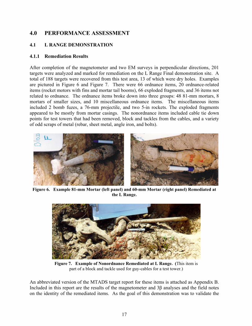
4.0 PERFORMANCE ASSESSMENT 4.1 L RANGE DEMONSTRATION 4.1.1 Remediation Results After completion of the magnetometer and two EM surveys in perpendicular directions, 201 targets were analyzed and marked for remediation on the L Range Final demonstration site. A total of 188 targets were recovered from this test area, 13 of which were dry holes. Examples are pictured in Figure 6 and Figure 7. There were 66 ordnance items, 20 ordnance-related items (rocket motors with fins and mortar tail booms), 66 exploded fragments, and 36 items not related to ordnance. The ordnance items broke down into three groups: 48 81-mm mortars, 8 mortars of smaller sizes, and 10 miscellaneous ordnance items. The miscellaneous items included 2 bomb fuzes, a 76-mm projectile, and two 5-in rockets. The exploded fragments appeared to be mostly from mortar casings. The nonordnance items included cable tie down points for test towers that had been removed, block and tackles from the cables, and a variety of odd scraps of metal (rebar, sheet metal, angle iron, and bolts).

An abbreviated version of the MTADS target report for these items is attached as Appendix B. Included in this report are the results of the magnetometer and 3β analyses and the field notes on the identity of the remediated items. As the goal of this demonstration was to validate the

Figure 6. Example 81-mm Mortar (left panel) and 60-mm Mortar (right panel) Remediated at the L Range.

Figure 7. Example of Nonordnance Remediated at L Range. (This item is part of a block and tackle used for guy-cables for a test tower.)

18

utility of the 3β analysis for target classification, all remaining discussion focuses on that analysis. 4.1.2 Performance Data

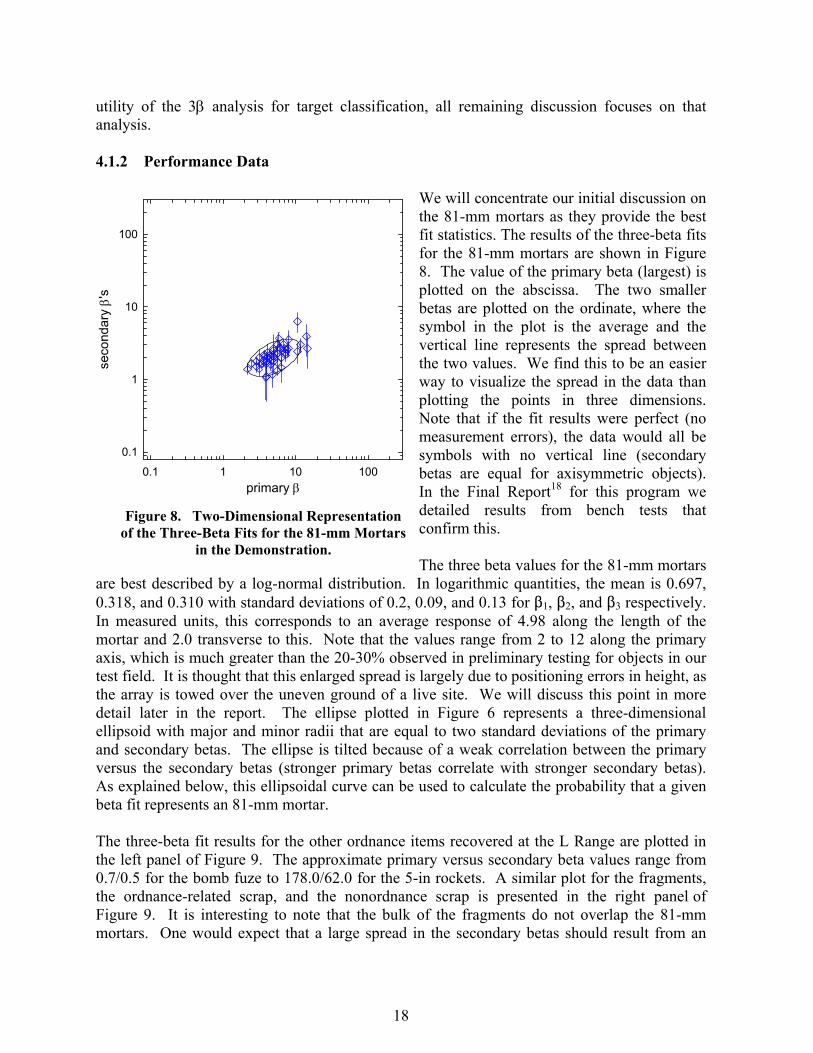
We will concentrate our initial discussion on the 81-mm mortars as they provide the best fit statistics. The results of the three-beta fits for the 81-mm mortars are shown in Figure 8. The value of the primary beta (largest) is plotted on the abscissa. The two smaller betas are plotted on the ordinate, where the symbol in the plot is the average and the vertical line represents the spread between the two values. We find this to be an easier way to visualize the spread in the data than plotting the points in three dimensions. Note that if the fit results were perfect (no measurement errors), the data would all be symbols with no vertical line (secondary betas are equal for axisymmetric objects). In the Final Report18 for this program we detailed results from bench tests that confirm this. The three beta values for the 81-mm mortars

are best described by a log-normal distribution. In logarithmic quantities, the mean is 0.697, 0.318, and 0.310 with standard deviations of 0.2, 0.09, and 0.13 for $1, $2, and $3 respectively. In measured units, this corresponds to an average response of 4.98 along the length of the mortar and 2.0 transverse to this. Note that the values range from 2 to 12 along the primary axis, which is much greater than the 20-30% observed in preliminary testing for objects in our test field. It is thought that this enlarged spread is largely due to positioning errors in height, as the array is towed over the uneven ground of a live site. We will discuss this point in more detail later in the report. The ellipse plotted in Figure 6 represents a three-dimensional ellipsoid with major and minor radii that are equal to two standard deviations of the primary and secondary betas. The ellipse is tilted because of a weak correlation between the primary versus the secondary betas (stronger primary betas correlate with stronger secondary betas). As explained below, this ellipsoidal curve can be used to calculate the probability that a given beta fit represents an 81-mm mortar. The three-beta fit results for the other ordnance items recovered at the L Range are plotted in the left panel of Figure 9. The approximate primary versus secondary beta values range from 0.7/0.5 for the bomb fuze to 178.0/62.0 for the 5-in rockets. A similar plot for the fragments, the ordnance-related scrap, and the nonordnance scrap is presented in the right panel of Figure 9. It is interesting to note that the bulk of the fragments do not overlap the 81-mm mortars. One would expect that a large spread in the secondary betas should result from an

primary β0.1 1 10 100

seco

ndar

y β'

s

0.1

1

10

100

Figure 8. Two-Dimensional Representation of the Three-Beta Fits for the 81-mm Mortars

in the Demonstration.

19

irregularly shaped object. Overall, the spread observed in the right panel of Figure 9 is not much greater than the spread for the axisymmetric ordnance objects (Figure 8 and left panel of Figure 9). After examining photos of the objects dug, this is not too surprising. Most of the scrap, to first order, is elongated, with approximately equal secondary dimensions.

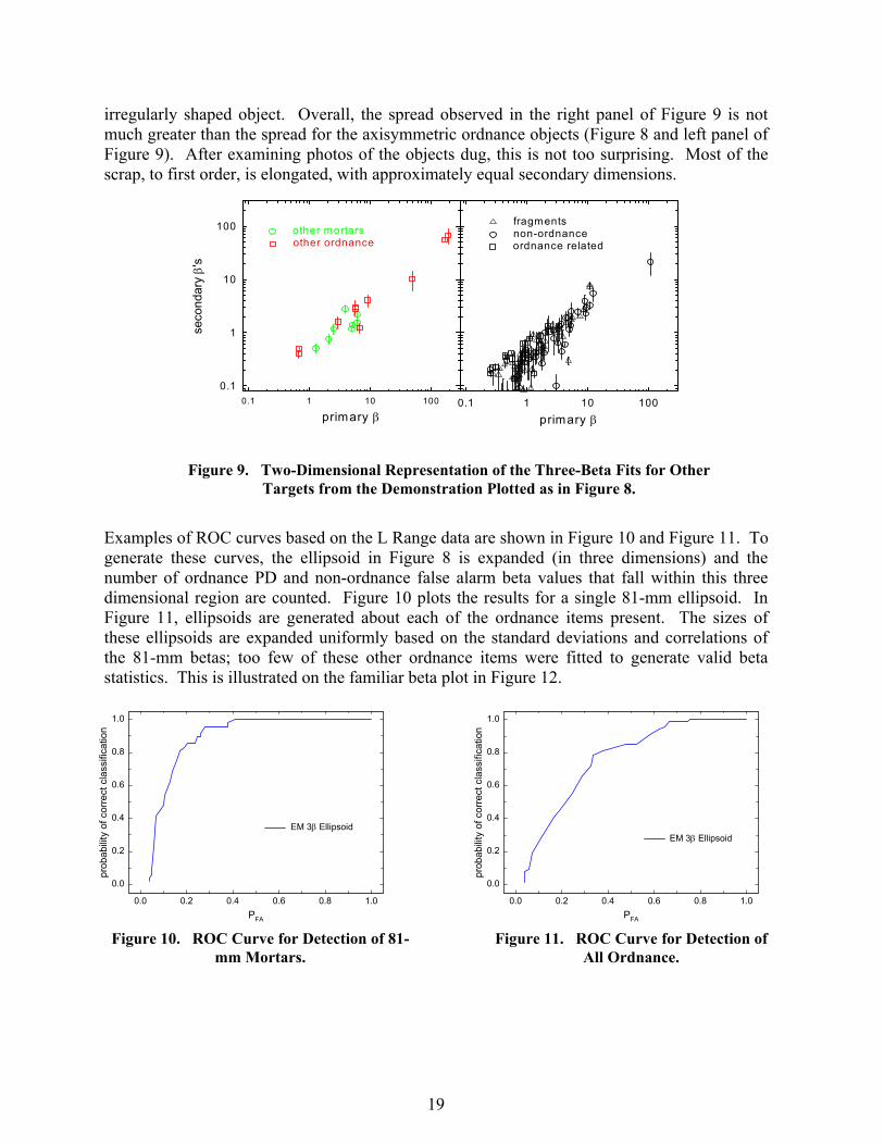
Examples of ROC curves based on the L Range data are shown in Figure 10 and Figure 11. To generate these curves, the ellipsoid in Figure 8 is expanded (in three dimensions) and the number of ordnance PD and non-ordnance false alarm beta values that fall within this three dimensional region are counted. Figure 10 plots the results for a single 81-mm ellipsoid. In Figure 11, ellipsoids are generated about each of the ordnance items present. The sizes of these ellipsoids are expanded uniformly based on the standard deviations and correlations of the 81-mm betas; too few of these other ordnance items were fitted to generate valid beta statistics. This is illustrated on the familiar beta plot in Figure 12.

Figure 9. Two-Dimensional Representation of the Three-Beta Fits for Other Targets from the Demonstration Plotted as in Figure 8.

PFA

0.0 0.2 0.4 0.6 0.8 1.0

prob

abilit

y of

cor

rect

cla

ssifi

catio

n

0.0

0.2

0.4

0.6

0.8

1.0

EM 3β Ellipsoid

primary β0.1 1 10 100

seco

ndar

y β'

s

0.1

1

10

100

primary β0.1 1 10 100

fragmentsnon-ordnanceordnance related

other mortarsother ordnance

Figure 10. ROC Curve for Detection of 81-mm Mortars.

Figure 11. ROC Curve for Detection of All Ordnance.

PFA

0.0 0.2 0.4 0.6 0.8 1.0

prob

abili

ty o

f cor

rect

cla

ssifi

catio

n

0.0

0.2

0.4

0.6

0.8

1.0

EM 3β Ellipsoid

20

The discrimination performance we achieve for a single ordnance item, 81-mm mortars, matches results we have obtained in earlier, controlled tests of this method. We achieve a roughly 60% reduction in false alarms without impacting PD. The story is more complicated when trying to discriminate several classes of ordnance from the background clutter (see Figure 11). We still reduce false alarms by 25%, but in order to identify the small fuzes in this field as ordnance, a large number of clutter items have to be included. In part, this is the inevitable result of trying to discriminate ordnance ranging in size from fuzes to 5-in rockets from clutter. This difficulty may be mitigated by obtaining more data, hence better fit statistics, on the smaller ordnance items. Using the error ellipsoid derived from the distribution of 81-mm mortar fits, as we were forced to do, may well overstate the region of the 3-D space occupied by the smaller ordnance items. As we obtain more model fits to remediated ordnance and improve our fit statistics, we will be able to test this premise. 4.1.3 Data Assessment The survey data collected during the first demonstration were of sufficient quality to meet the stated goals. We were able to increase the discrimination available using MTADS EM induction survey data for targets with isolated signatures. Several features of the data limited the classification ability, however. We showed in the earlier controlled tests that sensor noise and sensor location error limited the estimated betas to a precision of ~25%. Some improvement is possible in this regard, but not a lot. The GPS units used for sensor location on the MTADS array are state-of-the-art receivers with cm-level precision. Because of the response of the EM61 sensors to the GPS antenna, the antenna is located ~1.5 m in front of the sensor array. Although the antenna location is known to centimeters, there is some location uncertainty introduced by the back projection of the sensor locations from the antenna position.

primary β0.01 0.1 1 10 100

seco

ndar

y β'

s

0.01

0.1

1

10

100

81-mm mortars

clutterother ordnance

Mk 23

5-in

105-mm

Fuzes

81-mm

60-mm

Figure 12. Two-Dimensional Representation of the Three-Beta Fits to All Targets Dug in the Demonstration with Ellipses for Each Ordnance Class

Derived from the 81-mm Mortar Ellipse.

21

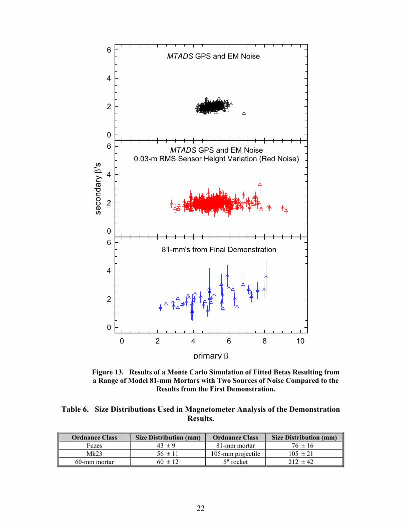
A two- or three-antenna array, with GPS antennas in front of and behind the EM sensors, would reduce sensor location uncertainties. At the time of this demonstration, this would have involved the purchase of another independent GPS receiver/radio combination. Now, because of the demand from the mining and construction markets, multiple receiver systems are available for a modest increase in price. Such a system was used at the second demonstration at the BBR impact area. Sensor noise is a different issue. Progress here requires a new generation of EM induction sensors. Compared to the data collected during our initial, controlled tests, there was a decrease in the precision of the fitted beta values during this demonstration. We attribute this to vertical motion of the EM array over the rough ground at the live site. In an attempt to provide some quantitative underpinning to this assertion, we have performed a Monte Carlo simulation of the fitted response of an 81-mm mortar simulant with varying sources of noise. The object used in the simulation had betas of 5,2,2, about that expected for an 81-mm mortar. The object was placed at a distance of 0.6 m from the sensor array and given a random x,y position relative to the survey tracks and a random orientation. Each simulation included real MTADS GPS and sensor noise. The results of this simulation are shown in Figure 13. The top panel shows the results using only GPS and sensor noise. In this case, the fitted betas exhibit just the precision observed in controlled tests, ~25%. For the simulation depicted in the bottom panel of Figure 11, a component of sensor height variation was added to simulate array bouncing over rough ground. We find that red noise with an root mean square (RMS) amplitude of 3 cm reproduces the spread in betas observed in the demonstration. This is easily within the realm of possibility; the MTADS EM array platform does not have a suspension and is observed to bounce in rough terrain. The terrain at the L Range demonstration was not especially rough for a live-site demonstration—MTADS has been demonstrated at several sites with much more challenging terrain. Therefore, to take advantage of the shape information inherent in the response of targets to the EM61 array, better control of vertical sensor displacements will be required. One option is to add suspension to the array platform. Another possibly more effective method would be to record the displacements of the array using inertial sensors and explicitly account for the position of the array in three dimensions in the data analysis procedure. 4.1.4 Technology Comparison The obvious baseline for comparison of the value of the technology demonstrated here is the current MTADS. As mentioned above, the baseline MTADS is able to achieve a reasonable level of discrimination using magnetometry fits alone, especially when the ordnance distribution is limited. We will compare the results obtained in this demonstration with those that would be obtained by MTADS at the same site so we have made use of the fitted magnetometer “size” parameter that is included in the target report in Appendix B. For each ordnance class, we calculate a mean size. Just as in the case of the 3-beta algorithm, we are able to calculate a distribution about this mean for the 81-mm mortars. We use the 81-mm size distribution to generate a proportionally-sized distribution for each ordnance class. The distributions derived are listed in Table 6.

22

0

2

4

6

seco

ndar

y β '

s

0

2

4

6

primary β

0 2 4 6 8 10

0

2

4

6

MTADS GPS and EM Noise

MTADS GPS and EM Noise0.03-m RMS Sensor Height Variation (Red Noise)

81-mm's from Final Demonstration

Table 6. Size Distributions Used in Magnetometer Analysis of the Demonstration

Results.

Ordnance Class Size Distribution (mm) Ordnance Class Size Distribution (mm) Fuzes 43 ± 9 81-mm mortar 76 ± 16 Mk23 56 ± 11 105-mm projectile 105 ± 21

60-mm mortar 60 ± 12 5" rocket 212 ± 42

Figure 13. Results of a Monte Carlo Simulation of Fitted Betas Resulting from a Range of Model 81-mm Mortars with Two Sources of Noise Compared to the

Results from the First Demonstration.

23

PFA

0.0 0.2 0.4 0.6 0.8 1.0

prob

abili

ty o

f cor

rect

cla

ssifi

catio

n

0.0

0.2

0.4

0.6

0.8

1.0

EM-FA vs EM-PD Mag SizeMag Size Ignoring Magnetized Objects

Figure 14. ROC Curve for Classification Using These Methods Compared to Results Using Magnetic

Dipole Size and Dipole Orientation.

We can then generate a ROC curve for this method by varying the width of the distribution around each ordnance class and declaring each target as ordnance (within the six size bands) or clutter. The result of this analysis is plotted in Figure 14. Also plotted in Figure 14 is a curve generated by enhancing the magnetometry analysis by taking advantage of the fitted magnetic dipole orientation for each target. This enhancement relies on the observation that UXO targets have, in general, been shock demagnetized by their impact with the ground and only exhibit induced magnetic moments while fragments and clutter have remanent moments. This was the case for the

ordnance recovered at the L Range; only one of the 73 items considered had a magnetic dipole orientation not consistent with an induced dipole only. Note that this method does not automatically eliminate all items with a remanent moment, only those whose net dipole orientation is outside that expected from an item with a wholly induced dipole. The magnetic dipole size suffers from many of the same problems as the 3-beta algorithm when attempting to discriminate all ordnance. In order to capture the fuzes, many small frag items must be included. The magnetic dipole orientation filter helps greatly in this regard as a good number of the frag items are magnetized and are thus correctly identified as clutter. It is difficult to compare the performance of the analysis of EM61 data presented here with that of other sensors and analysis methods. As we have shown, the current procedure gives excellent results in the test jig and reasonable results at our Test Field, which is a smooth, clean, and level site. The only legitimate comparison is to results obtained by competing technologies on live-site surveys. As these data become available, direct comparisons will follow. 4.2 BBR IMPACT AREA SURVEY 4.2.1 Pre-Demonstration Measurements As this demonstration was being planned, the manufacturer of the EM61, Geonics Limited, announced a new version of the sensor, designated the EM61 MkII. This new sensor has the ability to sample the decay of the induced magnetic fields with four independent gates compared to the two gates (one each on the upper and lower receive coils) in the EM61 MkI. This new product opens the possibility of gaining extra discrimination information by sampling a portion of the time-history of the object response coefficients, $. We incorporated this new instrument into the demonstration to test the utility of these new sampling gates.

24

Figure 15. Measured EM63 Response Profiles at Eight Time Gates from a Traverse over a Horizontal 105-mm Projectile

66 cm below the Sensor.

x (m)

-1.0 -0.5 0.0 0.5 1.0

EM

63 s

igna

l (m

V)

0.1

1

10

100

1000

MkII gates

16 ms

8 ms

4 ms

2 ms

The first step in incorporating the instrument into the MTADS suite of sensors was to specify the temporal positions of the gates. The instrument can be configured in one of two modes—all four gates on the lower receive coil or one on the upper coil and three on the lower. In order to maintain backward compatibility of the data with the EM61 MkI data, we elected to use the second mode with the sampling gate on the upper coil and the first sampling gate on the lower coil at the same time as the MTADS EM61 MkI gates. In order to gather the information required to make an intelligent choice for the later two gates in the MkII array, we leased an EM63 from Geonics for use at our Blossom Point Test Site. The EM63 can record the induced field decay in 26 time gates ranging out to beyond 20 milliseconds (ms). This instrument is not very amenable to vehicular use due to its low measurement rate, but it is ideal for accurately determining the complete decay response of test targets. We made measurements on the three projectiles expected to be encountered at the Badlands Bombing Range impact area—8-in, 155-mm, and 105-mm—as well as two frag clusters constructed by attaching pieces of frag recovered from the impact area in 1999 to styrofoam blocks to approximate the volume of the clusters encountered at the impact area. An example of the data collected on a 105-mm projectile is shown in Figure 15. These data are eight of the time gates collected during a traverse over a horizontal 105-mm projectile 66 cm below the sensor. The results are color coded into two classes, red for data from the four decay times that correspond to the sampling gates used in the standard MkII with four gates on the lower coil, and blue for later gates. As shown in the figure, the shape of the response begins to change clearly only for decay times greater than 2 ms. This change in shape is the result of longer-lived modes beginning to predominate as the short-lived modes decay.

25

Corresponding results for a frag cluster are shown in Figure 16. In this case, there is less variation of beta ratio with time, presumably because the measured response arises from the sum of many modes that decay with a range of decay times. Based on our measurements with the EM63, we initially specified a time for the latest gate in the MTADS EM61 MkII array of 2-5 ms. This number was a compromise between classification value which increases with increasing delay and signal to noise (S/N) which decreases as the antenna repetition rate is lowered to allow for later decay measurements. Unfortunately, due to some limitations of the design of their drive electronics, the latest gate Geonics could offer with an antenna repetition rate of 150 Hz was 1.2 ms. Rather than suffer the S/N consequences of lowering the repetition rate by a factor of 2, we settled for this relatively short gate for this demonstration. The actual gates available in the MTADS array for the two operating modes are listed in Table 7.

Table 7. Gate Times for the Two Modes of the MTADS EM61 MkIIs.

Operating Mode “4 on lower” “1 + 3” Upper Coil – Gate 1 280-465 µs Lower Coil – Gate 1 280-465 µs 280-465 µs Lower Coil – Gate 2 465-680 µs Lower Coil – Gate 3 680-925 µs 680-925 µs Lower Coil – Gate 4 925-1205 µs 925-1205 µs

Figure 16. Measured EM63 Response Profiles at Eight Time Gates from a Traverse over a Frag Cluster.

x (m)

-1.0 -0.5 0.0 0.5 1.0

EM63

sig

nal (

mV)

1

10

100

1000 MkII gates

16 ms

8 ms

4 ms

2 ms

26

430 440 450 460 470 480 490640

650

660

670

680

690

700

0 3150

430 440 450 460 470 480 490640

650

660

670

680

690

700

0 500

MkI U pper C oil MkII U pper C oil

430 440 450 460 470 480 490640

650

660

670

680

690

700

-25 35

mVmVMagnetometers

nT

4.2.2 Survey Data A conventional MTADS magnetometer survey of the seed area was conducted as the first survey at the demonstration site. Following analysis using the MTADS Data Analysis System, 170 targets were marked for remediation. Following the practice of the Jefferson Proving Ground (JPG) V demonstration, the targets were classified using a 6-bin scheme, where category 1 corresponds to high confidence ordnance, category 2 is medium confidence ordnance, category 3 is low confidence ordnance, category 4 is low confidence clutter, category 5 is medium confidence clutter, and category 6 is high confidence clutter. The analysts attempted to scale their rankings such that digging all category 1–5 targets would completely clear UXO from the site. A summary of the analysis results is shown in Table 8. These results serve as a baseline against which to compare the performance of the EM61 systems as well as the MTADS airborne system.

Table 8. Summary of the Magnetometer Analysis Results.

Category 1 2 3 4 5 6 TotalNumber of Targets 24 15 36 3 37 55 170

A North-South and an East-West EM61 MkII survey of the seed area were conducted as part of this demonstration as well as two orthogonal EM61 MkI surveys. A comparison of the results of the three surveys is shown for a small region of the Seeded Area in Figure 17.

Figure 17. Comparison of Results from All Three Surveys of the Seeded Area in a Small Subgrid. (The projectile targets are marked with diamonds for 105-mm and triangles for 155-mm.)

27

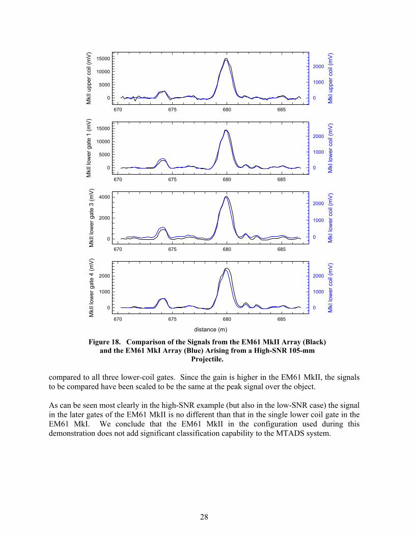
4.2.3 Data Assessment 4.2.3.1 EM61 MkII Electronic and Calibration Issues During initial examination of the MkII survey data, we discovered several features that compromised our ability to achieve reliable model fits. Between time gates on a single MkII and among the three MkII sensors in the array, discrepancies were found in the gain factors, the sampling times, and the noise levels. The MkII sensor measures the current in the transmit coil and uses this to normalize the output signal. This is done to maintain a constant output from the sensor as the battery voltage drops. When hooked up as an array of three sensors, one MkII is the master unit, and it triggers the two slave units. We initially noticed that the two slave sensors reported an odd oscillation of their transmit currents. Correcting the signal by these current variations caused their apparent signals to oscillate. Independent measurement of the transmit currents did not confirm these oscillations. In an array mode, the MkII sensors appear to have an electronic problem that causes an error in their current measurement circuitry. To correct for this, the current in the master sensor was used to normalize the signal in all three sensors. Even with this correction, problems were still observed with the relative outputs among the three sensors on the upper and lower coils and among the three time gates. A steel sphere was used as a calibration object to measure each sensor’s response, and correction gain factors were found for each sensor and time gate. These correction factors were as large as 25% between sensors. There was some indication that these factors may have been changing day to day. The MkI array was similarly calibrated, but had only minor corrections (10% between sensors) and appeared to be consistent from day to day. The MkI array was originally tested for timing problems between sensors by driving back and forth over a long wire or pipe. Each sensor was found to have a fixed timing offset needed to correctly map the data. Over time, these corrections have never been observed to vary. The same test with the MkIIs found similar timing offsets, but the offsets were found to vary from data file to data file. To correct for this, a “wire test” was performed in the field for each data file collected, and offsets were found for each file. Despite this added correction, there were still stretches of data collected where varying timing offsets were observed. The only conclusion is that the timing offsets change within a data file. Since the time of this demonstration, this sensor timing variation has been confirmed by other groups using the EM61 MkIIs. Finally, from data file to data file and day to day, the noise levels on certain sensors and certain time gates has been observed to change. At times, the noise was as much as five times greater. This noise dominated short time scales and was present even when the sensors were stationary. Given the inconsistent and unpredictable performance of the EM61 MkII discussed above, we must ask if there is enough new information in this sensor to justify the difficulty in using it. Figure 18 and Figure 19 show a comparison of the data collected by the EM61 MkII with that collected by the EM61 MkI over a high- and low-SNR 105mm projectile, respectively. In each of the figures, the upper coil signal is compared directly and the EM61 MkI lower coil signal is

28

670 675 680 685

MkI

I upp

er c

oil (

mV)

0

5000

10000

15000

MkI

upp

er c

oil (

mV

)

0

1000

2000

670 675 680 685

MkI

I low

er g

ate

1 (m

V)

0

5000

10000

15000

MkI

low

er c

oil (

mV)

0

1000

2000

670 675 680 685

MkI

I low

er g

ate

3 (m

V)

0

2000

4000

MkI

low

er c

oil (

mV

)

0

1000

2000

distance (m)

670 675 680 685

MkI

I low

er g

ate

4 (m

V)

0

1000

2000

MkI

low

er c

oil (

mV)

0

1000

2000

Figure 18. Comparison of the Signals from the EM61 MkII Array (Black) and the EM61 MkI Array (Blue) Arising from a High-SNR 105-mm

Projectile.

compared to all three lower-coil gates. Since the gain is higher in the EM61 MkII, the signals to be compared have been scaled to be the same at the peak signal over the object. As can be seen most clearly in the high-SNR example (but also in the low-SNR case) the signal in the later gates of the EM61 MkII is no different than that in the single lower coil gate in the EM61 MkI. We conclude that the EM61 MkII in the configuration used during this demonstration does not add significant classification capability to the MTADS system.

29

Figure 19. Comparison of the Signals from the EM61 MkII Array (Black) and the EM61 MkI Array (Blue) Arising from a Low-SNR 105-mm Projectile.

4.2.3.2 EM61 MkI Signal to Noise Ratios Three data rasters illustrating the relative noise levels at the Blossom Point test site, the Blossom Point “L” Range, and the BBR seed area are shown in Figure 20. This plot confirms the relative noise levels seen with the MkII between the Blossom Point test site and the BBR. Figure 21 is a power spectral density plot for the data from those two sites.

575 580 585 590 595

MkI

I upp

er c

oil (

mV)

-1000

0

1000

2000

3000

MkI

upp

er c

oil (

mV)

0

200

400

600

575 580 585 590 595

MkI

I low

er g

ate

1 (m

V)

0

1000

2000

3000

MkI

low

er c

oil (

mV

)

0

200

400

575 580 585 590 595

MkI

I low

er g

ate

3 (m

V)

-200

0

200

400

600

800

MkI

low

er c

oil (

mV

)

0

200

400

distance (m)

575 580 585 590 595

MkI

I low

er g

ate

4 (m

V)

0

200

400

MkI

low

er c

oil (

mV

)

0

200

400

30

0 10 20 30 40

uppe

r coi

l sig

nal (

mV)

-100

-50

0

50

100

150

200

0 10 20 30 40

uppe

r coi

l sig

nal (

mV)

-100

-50

0

50

100

150

200

distance (m)

0 10 20 30 40

uppe

r coi

l sig

nal (

mV)

-100

-50

0

50

100

150

200

Blossom Point Test Site

Blossom Point L-Range

BBR Impact Area

Figure 20. Comparison of the Noise Observed with the EM61 MkI at Three Sites.

frequency (Hz)0.1 1 10

PSD

mV2 /H

z

10-3

10-2

10-1

100

101

102

103

104

BBR Impact Area

Blossom Point Test Site

upper coillower coil

Figure 21. Power Spectral Density of the EM61 MkI Noise at Two Sites.

31

4.2.3.3 EM61 Model Fits The original goal of this demonstration was to invert the data over each anomaly and, using the beta response coefficients, to identify each ordnance item and discriminate the ordnance from the clutter. In all, 70 anomalies exhibited signal amplitudes at least twice the background. The peak EMI signatures ranged in amplitude from 400 to 9,000 mV (arbitrary units from Geonics EM61). Background variation over the scale lengths of the anomalies (several meters) was on the order of 100-200 mV, which, as seen in Figure 24 is much greater than at other sites we have surveyed. Of the seeded ordnance, three 105-mm, and one 155-mm did not meet this S/N threshold. The missed 105-mm were deeper than 0.5 m. The missed 155-mm was 0.85-m deep. The 8-in ranged in depth from 0.3 m to 0.75 m. Of the 37 nonordnance items analyzed, there were 19 clusters of exploded fragments, 12 individual pieces of shrapnel, and six pieces of scrap metal from the auto bodies used as targets. The results for all fits discussed in this Section are listed in Appendix C. The primary versus secondary fitted beta values for ordnance (left panel) and nonordnance (right panel) are shown in Figure 22. The symbols plot the primary beta value versus the average of the secondary values. The vertical line through each symbol indicates the maximum and minimum secondary beta values. Ideally for ordnance, the secondary beta values should be equal. The plotted circles are centered on the expected values for the betas of a 105-mm (solid), a 155-mm (dotted), and an 8-in (dashed). The circles are of equal radius on the log-log plots and in the left panel of Figure 22 contain all of the fitted ordnance items with a high S/N. These are shown with black symbols (105-mm as diamonds, 155-mm as squares, and 8-in as triangles). The red symbols in the left panel represent ordnance fits from low SNR data (peak signals less than 1,000 mV). These beta fits are far from the expected values. In the right panel of Figure 22, the symbols are green diamonds for fragment clusters, blue squares for single fragments, and pink triangles for scrap. The signals ranged in amplitude from 400 to 1,000 mV for the clusters, 500 to 2,000 mV for the singles, and 700 to 4,000 mV for the scrap. It should be noted that none of the nonordnance betas fall entirely within the high SNR ordnance spheres.

primary beta

0.1 1 10 100

seco

ndar

y be

tas

0.1

1

10

100

ordnance

primary beta

0.1 1 10 100

seco

ndar

y be

tas

0.1

1

10

100

non-ordnance

Figure 22. Plots of Primary Beta Versus Secondary Beta for Ordnance Items (left panel) and Clutter (right panel). (Circles represent regions containing high-SNR fits of

the three ordnance types. See the text for an explanation of the symbols.)

32

In an effort to understand these low SNR fit results, both data/model fits and normalized chi-square surfaces for a high SNR 155-mm, a low SNR 155-mm, and a fragment cluster are shown in Figure 23, Figure 24, and Figure 25. The data rasters plot the measured data from the center sensor as it passes directly over the object. The black line is the data, the symbols are data used in the fit, and the colored lines represent the best model fit to the data. The chi-square surfaces are a function of primary beta value and depth below ground and have been normalized in each case to the minimum chi-square. In the high SNR case, Figure 23, the data and model fit very closely at a primary beta value of 14, and the curvature of the chi-square contours is very steep. For the low SNR case, Figure 24, the curvature is not as steep indicating a larger uncertainty in the fitted model parameters. Indeed, two model fits are shown in Figure 24, one at the minimum chi-square (red plots) with a beta value of 6.3 and one at a primary beta value of 14 (green plots). The differences between these two fits and the data are comparable to the signal variation due to noise. A major factor in these poor inversions is the simple EMI signal shape from large ordnance. Because of the small ratio of primary to secondary beta for large ordnance (~1.3), the signals are a simple single peak response, and large variations in depth and primary beta produce very similar signal shapes.

distance (m)

-4 -2 0 2 4

cent

er s

enso

r (m

V)

0

500

1000

1500

2000

2500field datafit pointsmodel fit

primary β

0.1 1 10 100

dept

h (m

)0.0

0.2

0.4

0.6

0.8

1.0

Figure 23. Data Fit and Chi-Square Contours for a High-SNR 155-mm Projectile.

distance (m)

-4 -2 0 2 4

cent

er s

enso

r (m

V)

0

200

400

600field datafit pointsmodel fitconstrained fit

primary β

0.1 1 10 100

dept

h (m

)

0.0

0.2

0.4

0.6

0.8

1.0

Figure 24. Data Fit and Chi-Square Contours for a Low-SNR 155-mm Projectile.

33

Fragment clusters on the other hand, as shown in Figure 25, produce a broader merged two peak structure and typically show these features in any survey direction. This constrains the model to two large horizontal betas and a small vertical beta (βx = βy > βz). These are the betas expected from a flat axisymmetric plate.15 For this cluster, the betas were 12.5, 10.0, and 1.8. Even at low SNR, this two-peak structure remains significant, and the large spread in the secondary betas for all clusters can be seen in Figure 22. The normalized chi-square contours for this cluster are shown in the right panel of Figure 25. The curvature is not steep and the minimum is not well localized. This appears to be a result of the measured data simply not matching the model well no matter what the model parameters are. This poor match is not unexpected given that the signal comes from the sum of a number of small objects spread out over an area and not a single distinct metal object, which is what the model is based on.

4.2.3.4 An Alternate Discrimination Approach The consistent poor match between data and model for nonordnance fragment clusters suggests using a goodness-of-fit metric as a means of discriminating between ordnance and clutter. After considering several, the reduced chi-square was found to be an effective discriminant. For each fit, this quantity was calculated as the sum of the difference between model and data squared divided by the standard deviation of the noise squared and divided by the number of degrees of freedom. The noise was assumed to be roughly Gaussian with a standard deviation of 100 mV. Simple distributions of the background showed this only to be approximately true. The reduced chi-square as a function of peak signal for ordnance (left panel) and non-ordnance (right panel) is plotted in Figure 26. The colors and symbols denote the same items as in Figure 22. The dotted line denotes a straightforward means of discrimination by considering the ratio of the reduced chi-square to the peak signal.

distance (m)

-4 -2 0 2 4

cent

er s

enso

r (m

V)

0

200

400

600

800

1000field datafit pointsmodel fit

primary β

0.1 1 10 100

dept

h (m

)

0.0

0.2

0.4

0.6

0.8

1.0

Figure 25. Data Fit and Chi-Square Contours for a Frag Cluster.

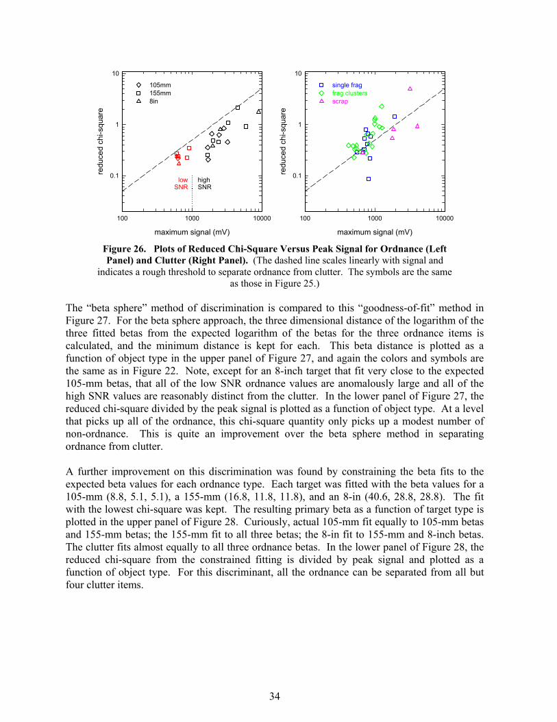
34

The “beta sphere” method of discrimination is compared to this “goodness-of-fit” method in Figure 27. For the beta sphere approach, the three dimensional distance of the logarithm of the three fitted betas from the expected logarithm of the betas for the three ordnance items is calculated, and the minimum distance is kept for each. This beta distance is plotted as a function of object type in the upper panel of Figure 27, and again the colors and symbols are the same as in Figure 22. Note, except for an 8-inch target that fit very close to the expected 105-mm betas, that all of the low SNR ordnance values are anomalously large and all of the high SNR values are reasonably distinct from the clutter. In the lower panel of Figure 27, the reduced chi-square divided by the peak signal is plotted as a function of object type. At a level that picks up all of the ordnance, this chi-square quantity only picks up a modest number of non-ordnance. This is quite an improvement over the beta sphere method in separating ordnance from clutter. A further improvement on this discrimination was found by constraining the beta fits to the expected beta values for each ordnance type. Each target was fitted with the beta values for a 105-mm (8.8, 5.1, 5.1), a 155-mm (16.8, 11.8, 11.8), and an 8-in (40.6, 28.8, 28.8). The fit with the lowest chi-square was kept. The resulting primary beta as a function of target type is plotted in the upper panel of Figure 28. Curiously, actual 105-mm fit equally to 105-mm betas and 155-mm betas; the 155-mm fit to all three betas; the 8-in fit to 155-mm and 8-inch betas. The clutter fits almost equally to all three ordnance betas. In the lower panel of Figure 28, the reduced chi-square from the constrained fitting is divided by peak signal and plotted as a function of object type. For this discriminant, all the ordnance can be separated from all but four clutter items.

maximum signal (mV)

100 1000 10000

redu

ced

chi-s

quar

e

0.1

1

10

maximum signal (mV)

100 1000 10000

redu

ced

chi-s

quar

e

0.1

1

10

105mm155mm8in

lowSNR

highSNR

single fragfrag clustersscrap

Figure 26. Plots of Reduced Chi-Square Versus Peak Signal for Ordnance (Left Panel) and Clutter (Right Panel). (The dashed line scales linearly with signal and

indicates a rough threshold to separate ordnance from clutter. The symbols are the same as those in Figure 25.)

35

3-be

ta s

pher

e di

scrim

inan

t0.01

0.1

1

10

object ID

0 10 20 30 40 50 60

redu

ced

chi-s

quar

e / S

max

1e-4

1e-3

1e-2

105-mm 155-mm 8-in frag cluster fragments scrap

Figure 27. Comparison of the Beta Sphere Discriminant to the Goodness-of-Fit Discriminant.

prim

ary

beta

1

10

100

object ID

0 10 20 30 40 50 60

redu

ced

chi-s

quar

e / S

max

1e-4

1e-3

1e-2

105-mm 155-mm 8-in frag cluster fragments scrap

Figure 28. Results of the Constrained Fits.

36

The ROC curves in Figure 29 compare the relative performance of these three methods. As the three discriminant levels are varied, the number of ordnance items correctly identified as ordnance (probability of detection) is plotted against the number of nonordnance items incorrectly identified as ordnance (probability of false alarm). The goodness-of-fit discriminant based on the constrained beta fits provides the best overall performance.

4.2.3.5 Technology Comparison The previous section showed the results of our analysis of the EM results obtained during the Impact Area survey and demonstrated in Figure 29 that the normalized χ2 from a constrained beta fit is the most effective discriminant. The baseline technology for comparison of these results is magnetometry. As mentioned in the Introduction, we have had considerable discrimination success when a skilled analyst fits magnetic anomalies and classifies the resulting targets. The magnetometry targets were categorized using the 6-bin priority (or confidence) scheme first introduced at JPG V and discussed above. The magnetometer data analysts attempted to scale their rankings such that digging all targets in categories 1-5 would clear all UXO from the site.19 The model parameters resulting from the magnetometry analysis were also submitted to the PNN developed in the NRL/Blackhawk SERDP program. This neural net was trained using test pit measurements on the three ordnance types emplaced in the seed area. Figure 30 shows a set of ROC curves comparing the performance of the constrained beta fit discriminant with those of the two magnetometry analyses. In contrast to Figure 29,

PFA

0.0 0.2 0.4 0.6 0.8 1.0

PD

0.0

0.2

0.4

0.6

0.8

1.0

number of clutter items

0 10 20 30

num

ber o

f ord

nanc

e

0

5

10

15

20

25

3β sphere3β reduced-χ2/Smax

constrained reduced-χ2/Smax

Figure 29. ROC Curves Comparing the Discrimination Performance of the Three Methods.

37

the abscissa of this plot is false alarms per hectare. Since the two methods detected a different number of objects, this is the only way to make a meaningful comparison. The most obvious point from Figure 30 is that the EMI system detected only 22 of the 26 ordnance items in the seed area. As discussed above, this is a function of the high noise in the EMI survey data. This noise arises from the near-saturation coverage of small frag pieces on this site to which the EMI system is much more sensitive. One obvious way to reduce this frag problem is to collect data at later times, after the contribution from the small frag pieces has decayed away. We discussed above the reasons this approach is not possible with the standard EM61 MkII that we deployed for this demonstration.

FA per hectare

0 10 20 30 40

P d

0.0

0.2

0.4

0.6

0.8

1.0

EM constrained fitanalyst's mag fitsPNN analysis of mag fits

Figure 30. ROC Curves Comparing the Discrimination Performance of the Constrained Beta Fit with the Two Magnetometry Analyses Used in this Demonstration.

This page left blank intentionally.

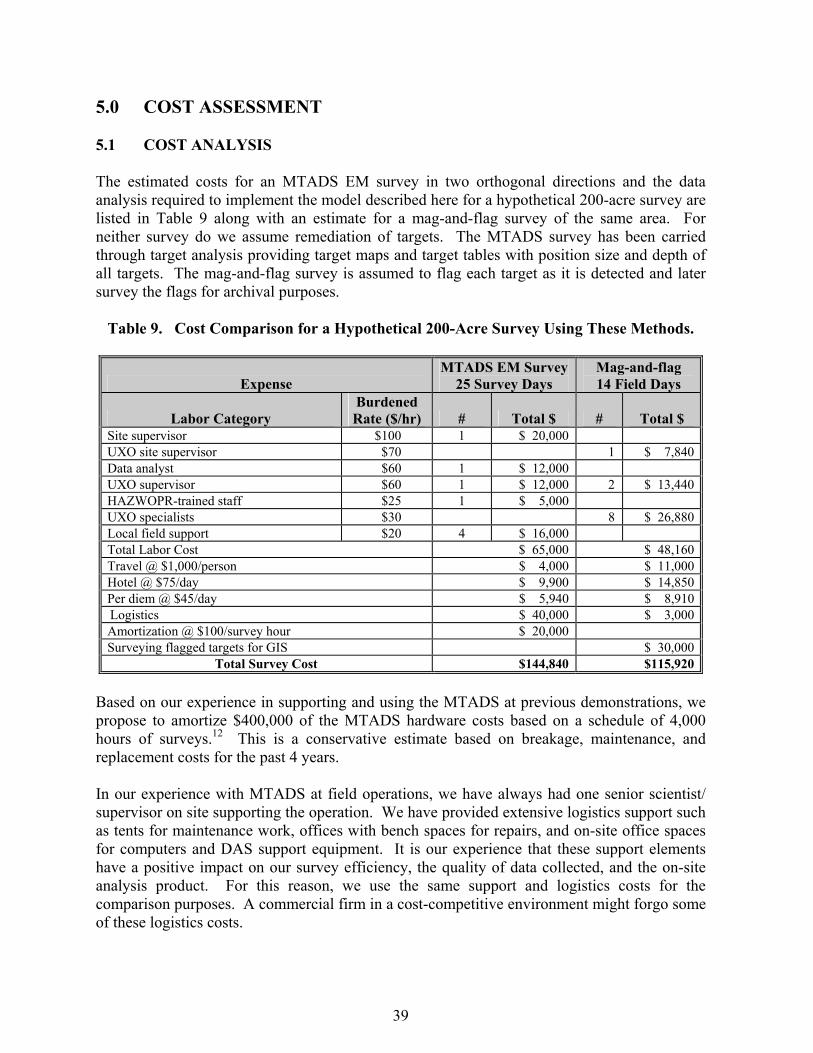
39

5.0 COST ASSESSMENT 5.1 COST ANALYSIS The estimated costs for an MTADS EM survey in two orthogonal directions and the data analysis required to implement the model described here for a hypothetical 200-acre survey are listed in Table 9 along with an estimate for a mag-and-flag survey of the same area. For neither survey do we assume remediation of targets. The MTADS survey has been carried through target analysis providing target maps and target tables with position size and depth of all targets. The mag-and-flag survey is assumed to flag each target as it is detected and later survey the flags for archival purposes.

Table 9. Cost Comparison for a Hypothetical 200-Acre Survey Using These Methods.

Expense MTADS EM Survey

25 Survey Days Mag-and-flag 14 Field Days

Labor Category Burdened Rate ($/hr) # Total $ # Total $

Site supervisor $100 1 $ 20,000 UXO site supervisor $70 1 $ 7,840Data analyst $60 1 $ 12,000 UXO supervisor $60 1 $ 12,000 2 $ 13,440HAZWOPR-trained staff $25 1 $ 5,000 UXO specialists $30 8 $ 26,880Local field support $20 4 $ 16,000 Total Labor Cost $ 65,000 $ 48,160Travel @ $1,000/person $ 4,000 $ 11,000Hotel @ $75/day $ 9,900 $ 14,850Per diem @ $45/day $ 5,940 $ 8,910Logistics $ 40,000 $ 3,000Amortization @ $100/survey hour $ 20,000 Surveying flagged targets for GIS $ 30,000

Total Survey Cost $144,840 $115,920 Based on our experience in supporting and using the MTADS at previous demonstrations, we propose to amortize $400,000 of the MTADS hardware costs based on a schedule of 4,000 hours of surveys.12 This is a conservative estimate based on breakage, maintenance, and replacement costs for the past 4 years. In our experience with MTADS at field operations, we have always had one senior scientist/ supervisor on site supporting the operation. We have provided extensive logistics support such as tents for maintenance work, offices with bench spaces for repairs, and on-site office spaces for computers and DAS support equipment. It is our experience that these support elements have a positive impact on our survey efficiency, the quality of data collected, and the on-site analysis product. For this reason, we use the same support and logistics costs for the comparison purposes. A commercial firm in a cost-competitive environment might forgo some of these logistics costs.

40

The MTADS survey costs include two orthogonal EM surveys only; no magnetometer survey is included. If large, deep targets were expected, a magnetometer survey would be required and an additional $50,000 would be necessary. Since two orthogonal EM surveys are included in the estimate while only one would be required for target detection, the added cost of these methods is $300 per acre. This is almost equal to the costs required to remediate one or two targets per acre. Thus, the economic break even point for the use of these methods is reached when three false alarms per acre are avoided. For the mag-and-flag operations, we assume that the number of personnel put on site is the number that can complete the survey in a 3-week period of performance. This minimizes the travel and logistics costs. The labor mix of UXO technicians to UXO supervisors and the site supervisor support and logistics support are typical of those that we have had quoted to support operations and also factor in information about labor rates and labor mixes typically quoted for operations similar to these. 5.2 COST COMPARISON These calculations, which show that the methods demonstrated here are 25% more costly on a per acre basis, do not address the ultimate goal of a particular survey: Is the survey being conducted to support remediation activities, or simply to provide an indication of whether the site is contaminated and the extent of the ordnance contamination? Previous studies of the detection efficiencies of mag-and-flag operations (at least for sites where ordnance exists below 1 meter in depth) have shown that most of ordnance remains undetected. Assuming that the survey is in support of a remediation activity, the cost per detected target is a useful comparison. Using documented mag-and-flag detection efficiencies of 35%,1 we find that these methods are more than twice as cost efficient at flagging ordnance for remediation. It should also be noted that following remediation based on a mag-and-flag survey 65% of the ordnance targets remain in the ground. Even these numbers do not take into account the false alarm reduction demonstrated in this survey. In the worst-case scenario, discriminating ordnance ranging from fuzes to 5-in shells from scrap, we were able to reject >20% of the false alarms without missing an ordnance target. With a more restricted target set, false alarm reductions of 33-50% are possible. Since a mag-and-flag survey has no significant classification ability, all targets have to be remediated. The true cost comparison of interest is a comparison of the results demonstrated by this method versus the baseline MTADS magnetometry analysis. A preliminary version of this comparison was attempted in the fall of 1999 at the Badlands Bombing Range impact area.18 The analysis described here was able to reject a number of false alarms that would have been marked for digging by the magnetometer analysis. The comparison is incomplete, however, as there was only one ordnance item detected in the area surveyed by the EM array. The second demonstration described here was undertaken to address this uncertainty. As shown in Figure 30, the initial slope of the ROC curve for our EM analysis is slightly steeper than the corresponding curve for the magnetometer analysis. This early advantage for these methods is overcome, however, by the fact that the EM system was able to achieve a high enough signal-to-noise ratio for reliable models fits for only 22 of the 26 ordnance items in the seed area.

41

6.0 REFERENCES 1. “Hand-held Gradiometer Survey Test at The Marine Corps Air Ground Combat Center,

Twentynine Palms, CA,” NAVEODTECHCEN TR, September 1992.

2. “MTADS TECHEVAL Demonstration, October 1996,” H. H. Nelson, J. R. McDonald, and Richard Robertson, NRL/PU/6110--97-348.

3. “Results of the MTADS Technology Demonstration #2, Magnetic Test Range, Marine

Corps Air Ground Combat Center, Twentynine Palms, CA, December 1996,” J. R. McDonald, H. H. Nelson, R. A. Jeffries, and Richard Robertson, NRL/PU/6110--97-349.

4. “Results of the MTADS Technology Demonstration #3, Jefferson Proving Ground,

Madison, IN, January 13-24, 1997,” H. H. Nelson, J. R. McDonald, R. A. Jeffries, and Richard Robertson, NRL/PU/6110--99-375.

5. “MTADS Unexploded Ordnance Operations at the Badlands Bombing Range, Pine

Ridge Reservation, Cuny Table, SD, July 1997,” J. R. McDonald, H. H. Nelson, J. Neece, Richard Robertson and R. A. Jeffries, NRL/PU/6110--98-353.

6. “MTADS Demonstration at the Former Fort Pierce Amphibious Base, Vero Beach, FL,

March 1998,” J. R. McDonald, H. H. Nelson, R. A. Jeffries, Richard Robertson, and K. Blankinship, NRL/PU/6110--98-372.

7. “MTADS Live Site Survey, Bombing Target #2 at the Former Buckley Field,

Arapahoe County, CO,” J. R. McDonald, H. H. Nelson and R. Robertson NRL/PU/6110--99-379.

8. “MTADS Geophysical Survey at The Jamaica Island and Topeka Pier Landfills at The

Portsmouth Naval Shipyard, Kittery, ME, October 1998,” J. R. McDonald, H. H. Nelson and B. Puc, NRL/PU/6110--99-381.

9. “MTADS Live Site Demonstration, Pueblo of Laguna, 6 July—7August 1998,” J. R.

McDonald, H. H. Nelson and R. A. Jeffries NRL/PU/6110--00-398.

10. “MTADS UXO Survey and Remediation on the Walker River Paiute Reservation, Schurz, NV, November 1998,” J. R. McDonald, H. H. Nelson, and R. A. Jeffries NRL/PU/6110--00-406.

11. “MTADS Geophysical Survey of Potential Underground Storage Tank Sites at the

Naval District Washington, Anacostia Annex,” H. H. Nelson, J. R. McDonald, R. Robertson, and B. Puc, NRL/MR/6110--00-8435.

12. ESTCP Cost and Performance Report. Multi-Sensor Towed Array Detection System.

September 1999. http://www.estcp.org/documents/techdocs/199526.pdf.

42

13. “Collection and Analysis of Multi-sensor Ordnance Signatures with MTADS,” Bruce Barrow and H. H. Nelson, J. Environ. Engineering Geophysics, 3, 71 (1998).

14. “Model-Based Characterization of EM Induction Signatures for UXO/Clutter

Discrimination Using the MTADS Platform,” Bruce Barrow and H. H. Nelson, Proceedings of the UXO Forum 1999, Atlanta, GA, May 25-27, 1999.

15. “Model-Based Characterization of EM Induction Signatures Obtained with the MTADS

EM Array,” Bruce Barrow and H. H. Nelson, IEEE Trans. Geophys. Remote Sens., 39, 1279 (2001).

16. “MTADS Unexploded Ordnance Operations at the Badlands Bombing Range Air Force

Retained Area, Pine Ridge Reservation, SD, September, 1999,” J. R. McDonald, H. H. Nelson, Richard Robertson and R. A. Jeffries, NRL/PU/6110--00-424.

17. “Draft Final Removal Report: Ordnance Removal at Army Research Laboratory,

Blossom Point Field Test Facility (BPFTF), Blossom Point, Maryland,” Human Factors Applications, Inc., DACA87-95-D-0027, Task Order 0008, 18 April 1997.

18. “Electromagnetic Induction and Magnetic Sensor Fusion for Enhanced UXO Target

Classification,” H. H. Nelson and Bruce Barrow, NRL/PU/6110--00-423.

19. “Airborne MTADS Demonstration on the Impact Area of the Badlands Bombing Range, September 2001,” J. R. McDonald, David Wright, Nagi Khadr, and H. H. Nelson, NRL/PU/6110--02-453.

A-1

APPENDIX A

POINTS OF CONTACT

Point of Contact Organization Phone/Fax/E-mail Role in Program Dr. Jeffrey Marqusee ESTCP 703-696-2120

703-696-2114 jeffrey.marqusee@osd.mil

ESTCP Director

Dr. Anne Andrews ESTCP 703-696-3826 703-696-2114 anne.andrews@osd.mil

Program Manager, UXO

Jeffrey Fairbanks ESTCP 703-736-4514 703-471-4180 jef@hgl.com

Program Assistant for UXO

Dr. Herbert Nelson Naval Research Laboratory Washington, DC

202-767-3686 202-404-8119 herb.nelson@nrl.navy.mil

Principal Investigator

Mr. Jack Kaiser Army Research Laboratory, Blossom Point

301-870-2329 301-870-3130 jkaiser@arl.mil

Blossom Point Site Manager

Mr. Bill Davis Army Research Laboratory, Blossom Point

301-394-2434 301-394-2514 wdavis@arl.mil

Explosives Safety Officer

Dr. Dan Steinhurst Nova Research, Inc. Alexandria, VA

202-767-3556 202-404-8119 das@ccs.nrl.navy.mil

Project Scientist

Mr. Glenn Harbaugh Nova Research, Inc. Alexandria, VA

301-392-1702 301-870-3130 glennquelmd@aol.com

Site Safety Officer

Dr. Tom Bell AETC, Inc. Arlington, VA

703-413-0500 703-413-0505 tbell@va.aetc.com

Project Manager

Dr. Bruce Barrow AETC, Inc. Arlington, VA

703-413-0500 703-413-0505 bjb@va.aetc.com

Project Scientist

Dr. J. R. McDonald AETC, Inc. Raleigh, NC

919-653-0215 919-653-0219 jimrmcdonald@nc.rr.com

Project Scientist

This page left blank intentionally.

APPENDIX B

MTADS TARGET REPORT FROM THE L RANGE DEMONSTRATION

This page left blank intentionally.

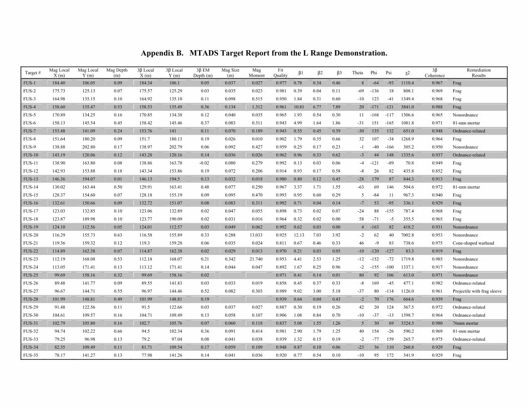
Appendix B. MTADS Target Report from the L Range Demonstration.

Target # Mag Local X (m)

Mag Local Y (m)

Mag Depth (m)

3$ Local X (m)

3$ Local Y (m)

3$ EM Depth (m)

Mag Size (m)

Mag Moment

Fit Quality $1 $2 $3 Theta Phi Psi χ2 3$

Coherence Remediation

Results FUS-1 184.40 106.05 0.09 184.34 106.1 0.05 0.037 0.027 0.977 0.78 0.34 0.46 8 -64 -93 1110.4 0.967 Frag

FUS-2 175.73 125.13 0.07 175.57 125.29 0.03 0.035 0.023 0.981 0.39 0.04 0.11 -69 -136 18 808.1 0.969 Frag

FUS-3 164.98 135.15 0.10 164.92 135.18 0.11 0.098 0.515 0.950 1.84 0.31 0.60 -10 123 -41 1349.4 0.968 Frag

FUS-4 158.60 135.47 0.53 158.53 135.49 0.36 0.134 1.312 0.961 10.81 6.77 7.89 20 -171 -121 3841.0 0.988 Frag

FUS-5 170.89 134.25 0.16 170.85 134.38 0.12 0.040 0.035 0.965 1.93 0.54 0.30 11 -168 -117 1306.6 0.965 Nonordnance

FUS-6 158.13 145.54 0.45 158.42 145.46 0.37 0.083 0.311 0.943 4.99 1.64 1.86 -31 151 -165 1081.8 0.971 81-mm mortar

FUS-7 153.48 141.09 0.24 153.76 141 0.11 0.070 0.189 0.943 0.55 0.45 0.39 -30 135 132 651.0 0.948 Ordnance-related

FUS-8 151.64 180.20 0.09 151.7 180.13 0.19 0.026 0.010 0.902 1.79 0.35 0.66 32 107 -34 1268.9 0.964 Frag

FUS-9 138.88 202.80 0.17 138.97 202.79 0.06 0.092 0.427 0.959 0.25 0.17 0.23 -1 -40 -166 305.2 0.950 Nonordnance

FUS-10 143.19 120.06 0.12 143.28 120.16 0.14 0.036 0.026 0.962 0.96 0.33 0.62 -3 44 148 1335.6 0.937 Ordnance-related

FUS-11 138.90 163.80 0.08 138.86 163.78 -0.02 0.080 0.279 0.992 0.13 0.03 0.06 -4 -121 -89 70.8 0.949 Frag

FUS-12 142.93 153.88 0.18 143.34 153.86 0.19 0.072 0.206 0.914 0.93 0.17 0.58 -8 26 82 435.8 0.852 Frag

FUS-13 146.36 194.07 0.01 146.13 194.5 0.13 0.032 0.018 0.980 0.80 0.12 0.45 -28 179 87 844.3 0.913 Frag

FUS-14 130.02 163.44 0.50 129.91 163.41 0.48 0.077 0.250 0.967 3.37 1.71 1.55 -63 69 146 504.6 0.972 81-mm mortar

FUS-15 128.37 154.60 0.07 128.18 155.19 0.09 0.095 0.470 0.993 0.95 0.60 0.29 5 -84 11 967.3 0.940 Frag

FUS-16 132.61 150.66 0.09 132.72 151.07 0.08 0.083 0.311 0.992 0.71 0.04 0.14 -7 53 -95 336.1 0.929 Frag

FUS-17 123.03 132.85 0.10 123.06 132.89 0.02 0.047 0.055 0.898 0.73 0.02 0.07 -24 88 -155 787.4 0.968 Frag

FUS-18 123.87 189.98 0.10 123.77 190.09 0.02 0.031 0.016 0.964 0.32 0.02 0.00 58 -71 -5 355.5 0.965 Frag

FUS-19 124.10 112.56 0.05 124.01 112.57 0.03 0.049 0.062 0.992 0.62 0.03 0.00 4 -163 82 418.2 0.931 Nonordnance

FUS-20 116.29 155.73 0.63 116.58 155.89 0.33 0.288 13.033 0.925 12.13 7.03 3.92 -2 62 40 7002.8 0.953 Nonordnance

FUS-21 119.36 159.32 0.12 119.3 159.28 0.06 0.035 0.024 0.811 0.67 0.46 0.33 46 -9 83 738.6 0.975 Cone-shaped warhead

FUS-22 114.89 162.38 0.07 114.87 162.38 0.02 0.029 0.013 0.970 0.21 0.03 0.05 -10 -120 -127 83.3 0.919 Frag

FUS-23 112.19 168.08 0.53 112.18 168.07 0.21 0.342 21.740 0.953 4.41 2.53 1.25 -12 -152 -72 1719.8 0.985 Nonordnance

FUS-24 113.05 171.41 0.13 113.12 171.41 0.14 0.044 0.047 0.892 1.67 0.25 0.96 -2 -155 -100 1337.1 0.917 Nonordnance

FUS-25 99.69 158.16 0.32 99.69 158.16 0.02 0.971 0.41 0.14 0.01 80 92 106 613.0 0.971 Nonordnance

FUS-26 89.48 141.77 0.09 89.55 141.83 0.03 0.033 0.019 0.858 0.45 0.37 0.33 -8 169 -45 477.1 0.982 Ordnance-related

FUS-27 96.67 144.71 0.55 96.97 144.46 0.52 0.082 0.303 0.989 9.02 3.00 5.18 -37 80 -114 1126.0 0.961 Projectile with frag sleeve

FUS-28 101.99 148.81 0.49 101.99 148.81 0.19 0.939 0.64 0.04 0.43 -2 70 176 664.6 0.939 Frag

FUS-29 91.48 122.56 0.11 91.5 122.66 0.03 0.037 0.027 0.887 0.30 0.19 0.26 42 20 124 367.5 0.972 Ordnance-related

FUS-30 104.61 109.57 0.16 104.71 109.49 0.13 0.058 0.107 0.906 1.08 0.84 0.70 -10 -37 -13 1398.7 0.964 Ordnance-related

FUS-31 102.79 105.80 0.16 102.7 105.76 0.07 0.060 0.118 0.837 5.08 1.55 1.26 5 30 69 3324.5 0.980 76mm mortar

FUS-32 94.74 102.22 0.66 94.5 102.34 0.36 0.091 0.414 0.981 2.90 1.79 1.25 40 154 -26 590.2 0.969 81-mm mortar

FUS-33 79.25 96.98 0.13 79.2 97.04 0.08 0.041 0.038 0.939 1.32 0.15 0.19 -2 -77 159 265.7 0.975 Ordnance-related

FUS-34 82.35 109.49 0.11 81.71 109.54 0.17 0.059 0.109 0.948 0.87 0.10 0.06 -23 36 110 260.8 0.929 Frag

FUS-35 78.17 141.27 0.13 77.98 141.26 0.14 0.041 0.036 0.920 0.77 0.54 0.10 -10 95 172 341.9 0.929 Frag

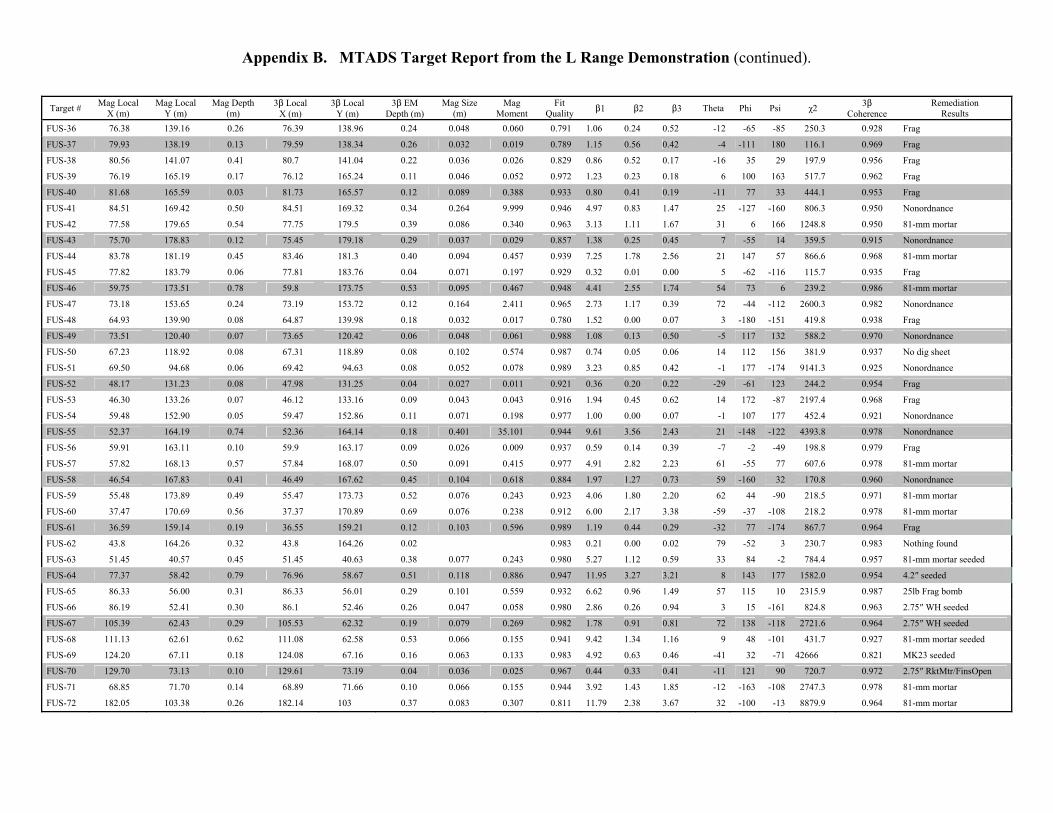
Appendix B. MTADS Target Report from the L Range Demonstration (continued).

Target # Mag Local X (m)

Mag Local Y (m)

Mag Depth (m)

3$ Local X (m)

3$ Local Y (m)

3$ EM Depth (m)

Mag Size (m)

Mag Moment

Fit Quality $1 $2 $3 Theta Phi Psi χ2 3$

Coherence Remediation

Results FUS-36 76.38 139.16 0.26 76.39 138.96 0.24 0.048 0.060 0.791 1.06 0.24 0.52 -12 -65 -85 250.3 0.928 Frag

FUS-37 79.93 138.19 0.13 79.59 138.34 0.26 0.032 0.019 0.789 1.15 0.56 0.42 -4 -111 180 116.1 0.969 Frag

FUS-38 80.56 141.07 0.41 80.7 141.04 0.22 0.036 0.026 0.829 0.86 0.52 0.17 -16 35 29 197.9 0.956 Frag

FUS-39 76.19 165.19 0.17 76.12 165.24 0.11 0.046 0.052 0.972 1.23 0.23 0.18 6 100 163 517.7 0.962 Frag

FUS-40 81.68 165.59 0.03 81.73 165.57 0.12 0.089 0.388 0.933 0.80 0.41 0.19 -11 77 33 444.1 0.953 Frag

FUS-41 84.51 169.42 0.50 84.51 169.32 0.34 0.264 9.999 0.946 4.97 0.83 1.47 25 -127 -160 806.3 0.950 Nonordnance

FUS-42 77.58 179.65 0.54 77.75 179.5 0.39 0.086 0.340 0.963 3.13 1.11 1.67 31 6 166 1248.8 0.950 81-mm mortar

FUS-43 75.70 178.83 0.12 75.45 179.18 0.29 0.037 0.029 0.857 1.38 0.25 0.45 7 -55 14 359.5 0.915 Nonordnance

FUS-44 83.78 181.19 0.45 83.46 181.3 0.40 0.094 0.457 0.939 7.25 1.78 2.56 21 147 57 866.6 0.968 81-mm mortar

FUS-45 77.82 183.79 0.06 77.81 183.76 0.04 0.071 0.197 0.929 0.32 0.01 0.00 5 -62 -116 115.7 0.935 Frag

FUS-46 59.75 173.51 0.78 59.8 173.75 0.53 0.095 0.467 0.948 4.41 2.55 1.74 54 73 6 239.2 0.986 81-mm mortar

FUS-47 73.18 153.65 0.24 73.19 153.72 0.12 0.164 2.411 0.965 2.73 1.17 0.39 72 -44 -112 2600.3 0.982 Nonordnance

FUS-48 64.93 139.90 0.08 64.87 139.98 0.18 0.032 0.017 0.780 1.52 0.00 0.07 3 -180 -151 419.8 0.938 Frag

FUS-49 73.51 120.40 0.07 73.65 120.42 0.06 0.048 0.061 0.988 1.08 0.13 0.50 -5 117 132 588.2 0.970 Nonordnance

FUS-50 67.23 118.92 0.08 67.31 118.89 0.08 0.102 0.574 0.987 0.74 0.05 0.06 14 112 156 381.9 0.937 No dig sheet

FUS-51 69.50 94.68 0.06 69.42 94.63 0.08 0.052 0.078 0.989 3.23 0.85 0.42 -1 177 -174 9141.3 0.925 Nonordnance

FUS-52 48.17 131.23 0.08 47.98 131.25 0.04 0.027 0.011 0.921 0.36 0.20 0.22 -29 -61 123 244.2 0.954 Frag

FUS-53 46.30 133.26 0.07 46.12 133.16 0.09 0.043 0.043 0.916 1.94 0.45 0.62 14 172 -87 2197.4 0.968 Frag

FUS-54 59.48 152.90 0.05 59.47 152.86 0.11 0.071 0.198 0.977 1.00 0.00 0.07 -1 107 177 452.4 0.921 Nonordnance

FUS-55 52.37 164.19 0.74 52.36 164.14 0.18 0.401 35.101 0.944 9.61 3.56 2.43 21 -148 -122 4393.8 0.978 Nonordnance

FUS-56 59.91 163.11 0.10 59.9 163.17 0.09 0.026 0.009 0.937 0.59 0.14 0.39 -7 -2 -49 198.8 0.979 Frag

FUS-57 57.82 168.13 0.57 57.84 168.07 0.50 0.091 0.415 0.977 4.91 2.82 2.23 61 -55 77 607.6 0.978 81-mm mortar

FUS-58 46.54 167.83 0.41 46.49 167.62 0.45 0.104 0.618 0.884 1.97 1.27 0.73 59 -160 32 170.8 0.960 Nonordnance

FUS-59 55.48 173.89 0.49 55.47 173.73 0.52 0.076 0.243 0.923 4.06 1.80 2.20 62 44 -90 218.5 0.971 81-mm mortar

FUS-60 37.47 170.69 0.56 37.37 170.89 0.69 0.076 0.238 0.912 6.00 2.17 3.38 -59 -37 -108 218.2 0.978 81-mm mortar

FUS-61 36.59 159.14 0.19 36.55 159.21 0.12 0.103 0.596 0.989 1.19 0.44 0.29 -32 77 -174 867.7 0.964 Frag

FUS-62 43.8 164.26 0.32 43.8 164.26 0.02 0.983 0.21 0.00 0.02 79 -52 3 230.7 0.983 Nothing found

FUS-63 51.45 40.57 0.45 51.45 40.63 0.38 0.077 0.243 0.980 5.27 1.12 0.59 33 84 -2 784.4 0.957 81-mm mortar seeded

FUS-64 77.37 58.42 0.79 76.96 58.67 0.51 0.118 0.886 0.947 11.95 3.27 3.21 8 143 177 1582.0 0.954 4.2″ seeded

FUS-65 86.33 56.00 0.31 86.33 56.01 0.29 0.101 0.559 0.932 6.62 0.96 1.49 57 115 10 2315.9 0.987 25lb Frag bomb

FUS-66 86.19 52.41 0.30 86.1 52.46 0.26 0.047 0.058 0.980 2.86 0.26 0.94 3 15 -161 824.8 0.963 2.75″ WH seeded

FUS-67 105.39 62.43 0.29 105.53 62.32 0.19 0.079 0.269 0.982 1.78 0.91 0.81 72 138 -118 2721.6 0.964 2.75″ WH seeded

FUS-68 111.13 62.61 0.62 111.08 62.58 0.53 0.066 0.155 0.941 9.42 1.34 1.16 9 48 -101 431.7 0.927 81-mm mortar seeded

FUS-69 124.20 67.11 0.18 124.08 67.16 0.16 0.063 0.133 0.983 4.92 0.63 0.46 -41 32 -71 42666 0.821 MK23 seeded

FUS-70 129.70 73.13 0.10 129.61 73.19 0.04 0.036 0.025 0.967 0.44 0.33 0.41 -11 121 90 720.7 0.972 2.75″ RktMtr/FinsOpen

FUS-71 68.85 71.70 0.14 68.89 71.66 0.10 0.066 0.155 0.944 3.92 1.43 1.85 -12 -163 -108 2747.3 0.978 81-mm mortar

FUS-72 182.05 103.38 0.26 182.14 103 0.37 0.083 0.307 0.811 11.79 2.38 3.67 32 -100 -13 8879.9 0.964 81-mm mortar

Appendix B. MTADS Target Report from the L Range Demonstration (continued).

Target # Mag Local X (m)

Mag Local Y (m)

Mag Depth (m)

3$ Local X (m)

3$ Local Y (m)

3$ EM Depth (m)

Mag Size (m)

Mag Moment

Fit Quality $1 $2 $3 Theta Phi Psi χ2 3$

Coherence Remediation

Results FUS-73 168.12 114.90 0.07 167.77 114.62 0.06 0.091 0.409 0.993 0.43 0.29 0.22 0 34 44 352.3 0.968 Frag

FUS-74 168.27 145.56 0.10 168.68 145.74 0.26 0.074 0.219 0.970 2.06 1.44 0.95 -6 176 154 1537.9 0.920 No dig sheet

FUS-75 151.38 155.44 0.11 151.41 155.67 0.14 0.037 0.028 0.957 0.69 0.49 0.53 -6 -180 10 1028.7 0.942 Bomb fuze

FUS-76 153.89 145.49 0.32 153.62 145.34 0.38 0.056 0.097 0.866 3.33 1.36 1.40 -11 36 178 776.0 0.950 Ordnance-related

FUS-77 153.21 158.10 0.30 153.29 157.32 0.19 0.087 0.363 0.945 1.26 0.19 0.50 13 -148 -141 307.1 0.970 Frag

FUS-78 133.95 187.04 0.44 133.95 187.04 0.14 0.986 8.95 2.97 4.95 10 26 79 7499.0 0.986 Nonordnance

FUS-79 133.94 191.98 0.37 133.63 191.89 0.44 0.073 0.213 0.956 5.64 1.76 2.82 40 -166 -114 1741.3 0.957 81-mm mortar

FUS-80 133.99 183 0.66 133.99 183 0.36 0.946 6.93 2.92 1.94 -21 -5 -152 2692.6 0.946 Nonordnance

FUS-81 129.53 190.78 0.08 129.33 190.8 0.08 0.080 0.280 0.969 0.34 0.26 0.06 -20 119 166 197.4 0.939 Frag

FUS-82 132.11 195.09 0.35 132.11 195.09 0.05 0.987 0.26 0.09 0.23 62 -11 -120 113.0 0.987 Nothing found

FUS-83 168.47 99.63 0.14 168.5 99.69 0.09 0.078 0.258 0.955 4.93 1.11 1.29 2 -113 -175 15748 0.953 Mortar

FUS-84 166.78 106.86 0.13 166.87 106.96 0.09 0.059 0.109 0.972 0.69 0.11 0.18 -82 158 4 868.2 0.981 Nonordnance

FUS-85 164.90 107.62 0.14 164.86 107.61 0.32 0.112 0.765 0.915 6.15 2.01 1.08 13 90 -160 3501.3 0.918 81-mmIll section

FUS-86 165.32 120.7 0.56 165.32 120.7 0.26 0.944 1.46 0.41 1.04 -25 113 -76 562.9 0.944 Frag

FUS-87 165.3 124.12 0.42 165.3 124.12 0.12 0.967 1.05 0.13 0.70 -24 124 170 1616.5 0.967 Frag

FUS-88 149.67 111.73 0.33 149.67 111.73 0.03 0.952 0.62 0.11 0.15 71 24 -69 2960.4 0.952 Ordnance-related

FUS-89 158.99 113.81 0.13 158.71 113.94 0.23 0.037 0.027 0.930 2.20 0.88 1.80 6 173 121 1199.2 0.963 Ordnance-related

FUS-90 157.74 117.69 0.21 158.11 117.53 0.37 0.042 0.040 0.902 2.26 2.04 0.45 20 -31 -24 1220.7 0.888 Frag

FUS-91 160.94 118.81 0.08 160.92 118.92 0.28 0.036 0.025 0.869 2.30 1.19 0.91 17 171 -83 2897.7 0.872 Ordnance-related

FUS-92 161.53 116.61 0.16 161.61 116.61 0.20 0.055 0.091 0.981 6.22 3.04 2.29 -5 -2 -5 6318.0 0.972 81-mm mortar

FUS-93 149.21 158.38 0.14 149.24 158.33 0.09 0.041 0.036 0.888 0.93 0.22 0.16 -15 13 -44 699.1 0.957 Frag

FUS-94 159.92 164.63 0.02 160.07 164.67 0.05 0.095 0.467 0.932 1.44 0.41 0.44 -9 135 137 1664.7 0.969 Frag

FUS-95 136.68 96.36 0.15 136.75 96.5 0.08 0.041 0.037 0.967 0.71 0.34 0.18 16 99 -137 848.1 0.920 2.75″ RktMtr

FUS-96 136.14 101.52 0.08 136.07 101.48 0.17 0.059 0.112 0.915 5.67 3.00 2.67 -10 28 -124 7030.2 0.981 Recoilless rifle round 76-80-mm/18″

FUS-97 137.75 149.22 0.13 137.83 149.16 0.17 0.052 0.075 0.940 2.70 1.28 0.96 -12 100 175 4276.5 0.939 Ordnance-related

FUS-98 138.74 147.83 0.25 138.5 147.65 0.39 0.148 1.747 0.960 4.83 0.25 0.35 6 95 113 599.5 0.924 Frag

FUS-99 137.71 146.32 0.19 137.4 146.24 0.09 0.043 0.044 0.747 0.65 0.22 0.05 -62 -52 108 1862.2 0.958 Frag

FUS-100 138.32 143.45 0.32 138.55 143.38 0.27 0.045 0.048 0.619 1.59 0.38 1.02 33 17 -77 648.4 0.938 Ordnance-related

FUS-101 140.33 175.30 0.07 140.3 175.27 0.13 0.090 0.397 0.997 0.47 0.02 0.12 5 -165 110 155.9 0.888 Frag

FUS-102 133.83 171.49 0.09 134.22 172.19 0.23 0.059 0.113 0.933 1.14 0.56 1.10 11 85 -100 500.0 0.945 Frag

FUS-103 137.26 191.92 0.13 137.26 191.87 0.18 0.065 0.152 0.985 3.30 1.51 0.84 20 81 -168 2616.2 0.975 Nonordnance

FUS-104 138.56 191.62 0.20 138.33 191.7 0.24 0.036 0.026 0.948 2.51 0.93 1.42 -13 -3 170 2155.4 0.966 60-mm mortar

FUS-105 136.68 189.81 0.26 136.7 189.87 0.24 0.062 0.132 0.960 5.65 1.53 1.13 18 36 41 2210.2 0.986 81-mm mortar

FUS-106 132.99 85.46 0.28 132.97 85.37 0.28 0.100 0.539 0.992 1.15 0.18 0.00 -50 56 113 744.1 0.928 Frag

FUS-107 126.83 94.48 0.54 126.76 94.45 0.45 0.243 7.832 0.859 189.02 45.23 89.93 2 -178 -77 815158 0.918 5″ Rkt

FUS-108 124.10 96.01 0.13 124.14 96.06 0.04 0.032 0.017 0.761 5.30 1.40 3.62 -45 119 127 71941 0.972 Nonordnance

FUS-109 130.87 112.16 0.40 131.36 112.59 0.07 0.110 0.728 0.693 7.47 1.98 2.02 -4 86 -47 21118.2 0.963 Frag

Appendix B. MTADS Target Report from the L Range Demonstration (continued).

Target # Mag Local X (m)

Mag Local Y (m)

Mag Depth (m)

3$ Local X (m)

3$ Local Y (m)

3$ EM Depth (m)

Mag Size (m)

Mag Moment

Fit Quality $1 $2 $3 Theta Phi Psi χ2 3$

Coherence Remediation

Results FUS-110 123.26 123.52 0.11 123.32 123.36 -0.01 0.041 0.036 0.940 0.25 0.15 0.20 9 -104 -123 451.4 0.950 Ordnance-related

FUS-111 129.01 123.99 0.21 128.91 124.09 0.16 0.072 0.200 0.922 0.92 0.20 0.73 5 130 -85 537.7 0.916 Frag

FUS-112 125.64 136.44 0.28 125.55 136.46 0.26 0.037 0.028 0.861 2.16 1.63 1.16 -55 101 -122 1391.3 0.980 81-mm mortar

FUS-113 128.76 136.30 0.11 128.69 136.25 0.10 0.042 0.041 0.925 0.47 0.34 0.26 -6 -10 -152 253.5 0.973 Nonordnance

FUS-114 123.54 162.86 0.22 123.5 162.74 0.17 0.103 0.585 0.936 4.18 0.65 0.56 1 72 -180 1404.7 0.966 Nonordnance

FUS-115 130.77 175.56 0.35 130.61 175.46 0.37 0.080 0.276 0.980 5.86 2.51 2.89 55 -163 117 1657.1 0.980 No dig sheet

FUS-116 122.95 175.89 0.08 122.84 175.9 0.27 0.040 0.035 0.986 3.75 0.57 0.31 2 -95 -9 1539.8 0.897 Nonordnance

FUS-117 119.33 166.90 0.44 119.51 166.9 0.37 0.087 0.352 0.958 7.60 2.00 3.20 33 -24 -143 6522.1 0.955 81-mm mortar

FUS-118 123.23 168.45 0.11 122.88 168.73 0.12 0.018 0.003 0.707 0.65 0.21 0.20 37 -124 -103 592.7 0.941 Frag

FUS-119 126.29 197.71 0.05 126.35 197.51 0.06 0.041 0.038 0.888 0.92 0.27 0.29 7 2 -46 427.6 0.965 Ordnance-related

FUS-120 133.84 204.27 0.09 133.88 204.32 0.11 0.051 0.074 0.968 0.58 0.38 0.28 41 165 120 398.5 0.970 Ordnance-related

FUS-121 113.27 78.31 0.17 113.62 78.29 0.27 0.061 0.122 0.877 1.77 0.33 0.20 1 -163 -12 340.4 0.905 Nonordnance

FUS-122 108.73 88.75 0.18 108.77 88.79 0.15 0.064 0.142 0.894 5.02 2.01 2.10 -3 57 -171 6490.4 0.979 81-mm mortar

FUS-123 111.67 100.19 0.11 111.51 100.22 0.13 0.087 0.355 0.902 0.84 0.26 0.48 -6 85 114 851.3 0.900 Frag

FUS-124 118.45 106.53 0.55 118.57 106.59 0.42 0.082 0.300 0.957 3.62 1.52 2.10 54 46 44 593.6 0.981 81-mm mortar

FUS-125 120.26 112.66 0.12 120.33 112.83 0.26 0.042 0.039 0.932 1.66 0.68 1.05 -7 -99 102 841.9 0.901 Ordnance-related

FUS-126 113.56 132.65 0.10 113.2 133.16 0.06 0.041 0.037 0.967 0.75 0.25 0.07 -73 43 -145 1025.2 0.976 Frag

FUS-127 106.36 134.57 0.11 106.34 134.66 0.22 0.084 0.321 0.792 1.08 0.05 0.06 -6 1 -56 387.6 0.868 Frag

FUS-128 120.67 135.58 0.11 120.66 135.43 0.34 0.064 0.143 0.910 3.05 0.04 0.16 -5 -110 1 802.8 0.859 Nonordnance

FUS-129 109.89 153.80 0.47 109.86 153.77 0.12 0.272 10.942 0.897 3.46 1.89 0.71 9 -121 101 4377.4 0.973 Nonordnance

FUS-130 111.49 163.56 0.27 111.42 163.58 0.18 0.066 0.153 0.983 4.57 1.83 1.35 -21 13 -50 2929.1 0.983 81-mm mortar

FUS-131 108.55 164.24 0.37 108.68 164.37 0.42 0.060 0.120 0.660 4.09 1.76 2.99 -44 126 -60 319.0 0.985 81-mm mortar

FUS-132 115.74 167.11 0.09 115.69 167.02 0.09 0.061 0.122 0.983 3.66 0.78 2.16 -5 -2 -107 5265.1 0.971 Nonordnance

FUS-133 89.84 190.89 0.10 89.7 190.91 0.13 0.082 0.299 0.985 1.26 0.61 0.41 5 74 0 776.5 0.954 60-mm mortar

FUS-134 88.15 184.29 0.06 88.15 184.31 -0.04 0.085 0.331 0.981 0.14 0.00 0.01 -7 -18 -38 51.9 0.926 Frag

FUS-135 91.05 177.83 0.04 91.11 177.85 0.06 0.049 0.063 0.984 1.46 0.70 0.27 8 -91 -17 660.7 0.978 Frag

FUS-136 91.11 175.62 0.12 90.88 175.14 0.06 0.071 0.198 0.957 0.28 0.10 0.23 27 66 127 281.1 0.959 Frag

FUS-137 93.82 174.63 0.59 93.88 174.45 0.27 0.337 20.752 0.956 4.66 1.31 2.46 34 -118 25 3925.3 0.961 Nonordnance

FUS-138 94.64 172.09 0.01 94.71 172.17 0.11 0.042 0.039 0.783 2.48 1.87 1.43 8 -87 -23 3358.2 0.968 81-mm nose section

FUS-139 96.03 178.16 0.24 95.25 177.14 0.30 0.095 0.466 0.703 5.31 2.14 1.29 8 -18 24 2296.5 0.933 Frag

FUS-140 101.05 171.69 0.25 100.98 171.81 0.22 0.154 1.983 0.988 17.28 9.43 13.14 -45 -24 -118 135963. 0.968 Frag

FUS-141 94.33 158.52 0.13 94.35 158.42 0.17 0.075 0.227 0.981 0.93 0.35 0.22 44 -58 -1 1256.7 0.946 Frag

FUS-142 90.06 157.56 0.65 90.08 157.5 0.35 0.357 24.791 0.970 9.33 2.85 1.71 -4 -171 -72 1929.7 0.971 Nonordnance

FUS-143 86.70 157.14 0.30 86.81 157.39 0.30 0.084 0.317 0.986 6.46 1.98 0.91 -42 -124 138 1979.0 0.985 81-mm mortar

FUS-144 92.85 157.30 0.11 92.71 156.53 0.02 0.064 0.143 0.917 0.47 0.02 0.07 47 -88 148 1563.3 0.948 Frag

FUS-145 96.22 151.97 0.53 96.08 152.07 0.30 0.329 19.350 0.977 10.73 2.71 3.75 10 -36 166 3283.4 0.970 Nonordnance

FUS-146 94.98 119.88 0.42 94.88 119.51 0.63 0.058 0.104 0.893 14.51 3.98 1.43 30 -86 34 3184.2 0.929 81-mm mortar

Appendix B. MTADS Target Report from the L Range Demonstration (continued).

Target # Mag Local X (m)

Mag Local Y (m)

Mag Depth (m)

3$ Local X (m)

3$ Local Y (m)

3$ EM Depth (m)

Mag Size (m)

Mag Moment

Fit Quality $1 $2 $3 Theta Phi Psi χ2 3$

Coherence Remediation

Results FUS-147 96.13 122.24 0.09 96.07 122.16 0.15 0.050 0.066 0.836 2.94 1.20 2.03 12 -59 -68 5986.2 0.911 Bomb fuze

FUS-148 91.29 117.57 0.75 90.92 117.31 0.98 0.130 1.187 0.968 48.84 14.22 6.10 27 -115 -133 1096.4 0.948 105-mm plus scrap

FUS-149 95.12 115.82 0.20 94.66 115.95 0.14 0.049 0.066 0.800 0.73 0.14 0.33 63 -172 -68 996.4 0.963 Frag

FUS-150 97.11 109.69 0.29 97.11 109.74 0.34 0.075 0.226 0.875 3.89 2.26 3.27 16 121 109 2661.4 0.943 4.2″ broke in half

FUS-151 97.63 94.70 0.02 97.54 94.72 0.07 0.057 0.098 0.850 4.45 1.42 1.69 10 62 126 9741.1 0.967 Frag

FUS-152 105.68 90.28 0.08 105.17 90.29 0.05 0.108 0.688 0.974 1.25 0.84 1.00 69 -7 -48 3833.6 0.971 Frag

FUS-153 92.88 72.93 0.22 92.89 72.68 0.29 0.078 0.257 0.829 3.76 2.15 2.03 30 12 66 1540.5 0.978 81-mm mortar

FUS-154 78.77 71.03 0.10 78.85 71.06 0.01 0.074 0.224 0.907 6.10 2.61 1.76 9 -97 -154 22986.3 0.984 81-mm Illum

FUS-155 81.02 76.06 0.19 81.05 76.19 0.19 0.083 0.315 0.943 4.66 2.28 1.41 42 33 170 11688.7 0.958 81-mm mortar

FUS-156 74.53 70.36 0.21 74.59 70.29 0.23 0.062 0.132 0.953 6.79 3.69 2.35 4 167 16 15916.3 0.925 81-mm mortar

FUS-157 76.18 72.49 0.09 76.16 72.55 0.12 0.045 0.049 0.977 3.20 1.44 0.60 1 54 -161 5657.4 0.936 Frag

FUS-158 84.51 86.96 0.17 84.59 86.91 0.13 0.032 0.018 0.964 2.01 0.51 0.86 -3 141 -91 1186.9 0.969 Frag

FUS-159 82.38 118.97 0.48 82.28 118.92 0.42 0.085 0.333 0.948 3.71 2.02 2.44 -52 9 92 654.3 0.983 81-mm mortar

FUS-160 79.13 114.53 0.45 78.86 114.35 0.47 0.070 0.186 0.906 5.17 1.93 2.60 43 -92 -93 1499.7 0.962 81-mm mortar

FUS-161 83.50 142.28 0.56 83.71 142.17 0.43 0.085 0.330 0.967 7.97 2.09 3.22 27 -12 58 2417.7 0.954 81-mm mortar

FUS-162 77.86 167.73 0.35 77.86 167.73 0.05 0.977 0.28 0.19 0.25 35 -128 160 164.6 0.977 Ordnance-related

FUS-163 75.37 173.65 0.12 75.3 173.86 0.05 0.045 0.049 0.827 0.86 0.54 0.70 16 55 44 803.8 0.976 Ordnance-related

FUS-164 83.62 173.63 0.78 83.95 173.19 0.86 0.332 19.820 0.886 41.23 0.00 40.33 -42 -116 44 10115.4 0.926 Nonordnance

FUS-165 74.88 182.53 0.64 74.73 182.7 0.41 0.073 0.212 0.905 3.91 0.53 1.62 8 -111 -10 1346.3 0.907 81-mm mortar

FUS-166 74.38 187.01 0.45 74.48 187.21 0.69 0.088 0.366 0.981 3.45 1.68 1.61 71 26 85 723.0 0.985 81-mm mortar

FUS-167 81.47 186.46 0.42 81.82 186.88 0.65 0.055 0.092 0.947 10.54 3.16 1.69 9 49 -58 695.7 0.915 81-mm mortar

FUS-168 83.42 188.39 0.55 83.52 188.68 0.84 0.293 13.672 0.941 28.63 2.85 0.00 54 45 122 11281.8 0.889 Nonordnance

FUS-169 63.84 185.26 0.56 63.88 185.31 0.47 0.077 0.250 0.973 2.85 1.98 1.57 59 -70 -56 240.6 0.989 81-mm mortar

FUS-170 64.40 183.25 0.38 64.39 183.12 0.42 0.067 0.165 0.950 7.23 2.62 2.11 26 -74 49 1755.0 0.970 81-mm mortar

FUS-171 66.42 182.07 0.51 66.75 182.18 0.75 0.073 0.215 0.981 4.80 0.78 1.53 35 151 114 314.0 0.969 81-mm mortar

FUS-172 58.50 170.57 0.25 60.68 170.58 0.58 0.244 7.842 0.772 8.29 3.11 2.13 -30 175 -148 592.3 0.967 Frag

FUS-173 62.97 170.42 0.09 62.96 170.35 0.11 0.124 1.026 0.731 3.94 1.13 0.54 -6 -127 155 1957.3 0.978 Frag

FUS-174 67.74 168.10 0.48 67.6 167.98 0.37 0.112 0.769 0.950 8.08 2.41 4.68 36 -117 -164 2574.6 0.983 81-mm mortar

FUS-175 65.69 157.17 0.04 65.65 157.21 0.11 0.036 0.025 0.792 0.97 0.73 0.55 12 99 174 1076.1 0.966 Frag

FUS-176 71.00 159.89 0.33 71.37 159.62 0.47 0.070 0.185 0.962 5.60 2.19 1.69 30 -51 -137 823.1 0.976 Frag

FUS-177 60.18 151.02 0.01 60.19 151 0.02 0.039 0.033 0.994 0.74 0.11 0.07 -3 -149 -177 752.4 0.945 Nonordnance

FUS-178 61.22 130.56 0.59 61.15 129.97 0.93 0.080 0.283 0.943 4.90 1.20 4.28 68 -122 -179 357.0 0.971 81-mm mortar

FUS-179 63.00 127.23 0.16 63.1 127.31 0.11 0.068 0.171 0.972 0.58 0.05 0.24 50 121 -159 960.4 0.957 Frag

FUS-180 60.93 116.11 0.63 60.8 116.24 0.40 0.098 0.512 0.947 3.97 2.37 1.20 23 124 -124 957.8 0.971 81-mm mortar

FUS-181 67.45 88.93 1.17 67.98 89.09 1.17 0.180 3.157 0.948 168.06 60.27 52.22 -6 32 -144 4173.4 0.931 8 Venturies

FUS-182 70.63 88.05 0.15 70.68 88.08 0.13 0.071 0.193 0.967 7.11 2.96 2.39 -6 -114 22 26947.1 0.949 81-mm mortar

FUS-183 71.12 85.62 0.37 71.09 85.64 0.36 0.270 10.704 0.846 106.81 11.72 31.51 -4 58 -6 914831. 0.869 Nonordnance

Appendix B. MTADS Target Report from the L Range Demonstration (continued).

Target # Mag Local X (m)

Mag Local Y (m)

Mag Depth (m)

3$ Local X (m)

3$ Local Y (m)

3$ EM Depth (m)

Mag Size (m)

Mag Moment

Fit Quality $1 $2 $3 Theta Phi Psi χ2 3$

Coherence Remediation

Results FUS-184 75.91 86.17 0.40 75.57 86.52 0.68 0.115 0.830 0.888 10.69 6.42 9.08 40 21 -97 1177.4 0.968 Frag

FUS-185 77.42 84.72 0.45 77.59 84.75 0.20 0.121 0.955 0.763 10.73 4.40 8.30 9 80 -101 42512.9 0.945 81-mm mortar

FUS-186 55.71 132.81 0.48 55.28 132.81 0.39 0.086 0.342 0.917 5.59 1.98 1.45 50 -154 106 1419.2 0.983 81-mm mortar

FUS-187 45.62 146.87 0.14 45.69 146.82 0.07 0.067 0.163 0.981 5.24 1.04 1.68 -13 132 -128 42751.7 0.922 Nonordnance

FUS-188 55.82 143.67 0.77 55.72 143.8 0.47 0.125 1.067 0.951 5.69 4.06 2.07 63 93 -20 999.3 0.978 15-25 frag bomb

FUS-189 54.79 150.73 0.42 54.86 150.67 0.34 0.089 0.383 0.977 6.32 2.48 1.51 40 -5 29 7431.4 0.948 81-mm mortar

FUS-190 50.89 140.98 0.12 50.77 141.02 0.15 0.029 0.014 0.838 1.39 0.37 0.49 0 -2 -129 457.5 0.966 Nonordnance

FUS-191 46.75 159.70 0.17 46.77 159.72 0.10 0.103 0.593 0.975 0.74 0.13 0.26 17 125 -96 227.4 0.957 Frag

FUS-192 51.15 179.35 0.50 51.31 179.58 0.43 0.077 0.249 0.936 4.91 1.90 2.21 15 38 -171 381.0 0.984 81-mm mortar

FUS-193 50.45 170.94 0.57 50.45 170.94 0.27 0.981 2.06 0.62 0.91 36 2 22 195.3 0.981 60-mm M720

FUS-194 44.21 175.55 0.60 44.13 175.3 0.52 0.074 0.217 0.957 3.96 0.50 1.73 42 -46 172 612.2 0.954 81-mm HE M371

FUS-195 45.83 172.30 0.55 45.71 172.28 0.53 0.073 0.214 0.961 3.13 1.47 2.59 -49 149 -170 342.4 0.974 81-mm mortar

FUS-196 40.04 176.63 0.07 40.01 176.76 0.21 0.036 0.025 0.798 2.61 1.17 1.63 11 -35 66 1977.6 0.967 Frag

FUS-197 35.78 175.99 0.36 35.87 176.09 0.50 0.061 0.124 0.928 5.57 3.77 2.31 37 -2 -31 604.1 0.975 81-mm mortar

FUS-198 29.47 176.71 0.33 29.59 176.63 0.37 0.057 0.101 0.958 5.90 2.84 4.43 -26 146 -91 1589.6 0.978 81-mm mortar

FUS-199 41.30 51.76 0.45 41.38 51.93 0.71 0.085 0.331 0.959 14.02 2.06 5.82 61 -20 166 9362.6 0.817 81-mm mortar

FUS-200 49.44 48.31 0.17 49.43 48.45 0.23 0.050 0.066 0.939 4.02 0.34 0.66 -2 -78 -116 1604.4 0.931 MK23 seeded

FUS-201 90.08 67.30 0.82 90.01 67.52 0.56 0.115 0.828 0.979 5.85 1.61 4.69 6 154 -32 1296.1 0.946 105-mm seeded

APPENDIX C

MTADS TARGET REPORT FROM THE BBR IMPACT AREA DEMONSTRATION

This page left blank intentionally.

Table C-1. Model Results for 105-mm Projectiles.

Magnetometer Fit 3-$ Fit

ID Local X (m)

Local Y (m)

Depth (m)

Size (m) Inclin. Az. Fit

Qual. Comments Cat. Local X (m)

Local Y (m)

Depth (m) Θ Φ Ψ $1 $2 $3

Fit Qual. χ2

13 389.49 548.04 0.66 0.125 71 261 0.952 poor degaussing, 105, nose down 2 389.44 547.73 0.35 -37 61 -47 12.1 4.2 5.9 0.981 8373

59 538.57 579.57 0.74 0.147 82 170 0.975 good fit for a 155 1 538.61 579.46 0.45 46 -139 -15 10.0 7.0 3.8 0.972 3567

99 507.18 585.20 0.91 0.141 74 222 0.969 105, nose down 1 507.06 584.88 0.60 28 -106 122 9.2 3.1 0.0 0.938 2189

133 474.58 656.87 0.67 0.117 55 251 0.960 105, slight remnant 2 474.67 656.84 0.37 24 47 -26 8.4 3.5 6.6 0.989 4528

142 512.94 679.83 0.61 0.101 34 30 0.954 105mm 1 512.92 679.85 0.31 -13 50 -125 8.4 5.2 6.5 0.980 6308

149 460.22 689.48 0.69 0.138 51 312 0.982 105/155mm, E/W, nose down 1 460.41 689.39 0.37 65 -51 -112 6.4 4.4 5.6 0.977 2063

163 434.35 711.40 0.67 0.135 47 299 0.972 155mm, E/W 1 434.40 711.43 0.62 9 138 160 6.5 4.2 5.5 0.979 6577

Constrained 3-$ Fit

ID Local X (m)

Local Y (m)

Depth (m) Θ Φ Ψ $1 $2 $3

Fit Qual. χ2 S1

(max)

13 389.52 547.88 0.53 88 42 46 16.8 11.8 11.8 0.966 15046 2859

59 538.74 579.55 0.46 73 -60 -175 8.8 5.1 5.1 0.968 4368 1680

99 507.05 585.24 0.77 81 -127 -150 8.8 5.1 5.1 0.919 3636 626

133 474.52 656.78 0.42 62 -129 -168 8.8 5.1 5.1 0.969 13215 3222

142 512.98 679.88 0.53 79 154 -54 16.8 11.8 11.8 0.965 11233 2432

149 460.39 689.41 0.63 87 -1 -162 16.8 11.8 11.8 0.959 4566 1697

163 434.39 711.39 0.89 85 95 133 16.8 11.8 11.8 0.968 11265 1913

Table C-2. Model Results for 155-mm Projectiles.

Magnetometer Fit 3-$ Fit

ID Local X (m)

Local Y (m)

Depth (m)

Size (m) Inclin. Az. Fit

Qual. Comments Cat. Local X (m)

Local Y (m)

Depth (m) Θ Φ Ψ $1 $2 $3

Fit Qual. χ2

86 383.80 601.67 0.73 0.217 -69 282 0.950 totally inverted, fence post 5 383.82 601.68 0.33 26 -111 -71 18.7 12.3 16.0 0.985 21187

88 429.63 581.65 0.86 0.204 75 355 0.947 good fit for 8in 1 429.67 581.65 0.43 15 -27 21 14.0 11.2 8.8 0.984 4818

104 539.83 624.56 0.85 0.164 31 28 0.974 155mm 1 539.95 624.51 0.43 5 -149 139 14.1 11.6 10.4 0.989 4608

109 482.37 621.69 1.12 0.209 72 270 0.956 8-in, E/W 1 481.80 621.61 0.89 -23 -16 24 55.0 37.0 15.2 0.903 3469

121 367.38 636.27 0.92 0.092 44 4 0.867 Clutter 6 367.60 635.55 0.46 11 -64 -119 6.0 2.4 1.3 0.889 2699

132 441.28 657.90 0.57 0.132 45 316 0.983 likely 105 1 441.20 657.91 0.51 -31 -25 -120 17.4 12.7 15.4 0.993 9137

135 500.78 651.99 1.03 0.133 69 54 0.874 105mm, nose down 1 500.70 651.86 0.64 37 -118 -166 19.8 10.9 14.6 0.986 2561

148 468.05 683.84 0.81 0.156 63 188 0.986 155mm 1 467.91 683.72 0.53 -9 -23 -167 25.8 8.4 15.3 0.984 10862

154 394.32 691.49 1.39 0.235 87 3 0.941 deep 8-in, nose down 1 394.14 691.43 1.05 -11 42 -77 23.6 9.5 4.3 0.913 2354

167 502.18 717.05 1.04 0.108 64 359 0.921 possible deep 105mm 2 502.10 716.87 1.00 1 17 -20 53.8 6.9 32.5 0.930 2239

Constrained 3-$ Fit

ID Local X (m)

Local Y (m)

Depth (m) Θ Φ Ψ $1 $2 $3

Fit Qual. χ2 S1

(max)

86 383.79 601.77 0.57 71 157 53 40.6 28.8 28.8 0.973 38105 4482

88 429.69 581.67 0.49 20 -27 -78 16.8 11.8 11.8 0.982 5248 1984

104 540.02 624.56 0.47 29 22 -4 16.8 11.8 11.8 0.986 5893 2405

109 481.95 621.85 0.70 16 123 -95 16.8 11.8 11.8 0.871 6584 901

121 367.52 635.82 0.75 77 145 172 8.8 5.1 5.1 0.755 5386 599

132 441.19 657.90 0.48 -45 -40 50 16.8 11.8 11.8 0.987 15631 5917

135 500.78 652.02 0.59 39 55 43 16.8 11.8 11.8 0.983 3052 1666

148 467.87 683.65 0.29 5 175 54 8.8 5.1 5.1 0.954 33511 3279

154 394.27 691.45 0.86 -8 35 149 8.8 5.1 5.1 0.862 3746 631

167 502.26 717.06 1.00 14 39 32 40.6 28.8 28.8 0.877 4311 854

Table C-3. Model Results for 8-in Projectiles.

Magnetometer Fit 3-$ Fit

ID Local X (m)

Local Y (m)

Depth (m)

Size (m) Inclin. Az. Fit

Qual. Comments Cat. Local X (m)

Local Y (m)

Depth (m) Θ Φ Ψ $1 $2 $3

Fit Qual. χ2

26 470.81 534.05 1.12 0.166 88 147 0.942 likely 155, nose down 1 470.92 534.06 0.66 25 12 -58 33.6 25.9 20.4 0.975 7905

89 415.36 597.87 0.76 0.192 29 15 0.962 155mm/8in, good target 1 415.33 597.83 0.41 39 -152 -108 43.0 33.1 35.9 0.993 17584

112 455.59 632.93 1.37 0.225 84 254 0.969 8-in deep 1 455.50 633.02 0.85 7 153 22 34.9 21.7 12.1 0.942 1726

139 538.84 657.89 1.12 0.210 70 84 0.981 8-in, E/W 1 538.99 657.88 0.74 32 72 57 37.1 28.0 28.6 0.981 3808

153 405.62 686.54 1.24 0.148 90 356 0.970 probable deep 155 1 405.50 686.62 0.88 10 90 8 10.2 6.5 3.5 0.919 2374

Constrained 3-$ Fit

ID Local X (m)

Local Y (m)

Depth (m) Θ Φ Ψ $1 $2 $3

Fit Qual. χ2 S1

(max)

26 470.96 534.03 0.73 41 18 -116 40.6 28.8 28.8 0.974 8554 2513

89 415.30 597.82 0.38 30 -145 73 40.6 28.8 28.8 0.992 19930 9027

112 455.67 632.84 1.01 10 -44 -113 40.6 28.8 28.8 0.886 3391 646

139 539.00 657.90 0.75 35 71 54 40.6 28.8 28.8 0.981 3799 1965

153 405.47 686.57 1.13 7 93 -138 16.8 11.8 11.8 0.893 3024 603

Table C-4. Model Results for Frag Clusters.

Magnetometer Fit 3-$ Fit

ID Local X (m)

Local Y (m)

Depth (m)

Size (m) Inclin. Az. Fit

Qual. Comments Cat. Local X (m)

Local Y (m)

Depth (m) Θ Φ Ψ $1 $2 $3

Fit Qual. χ2

12 387.73 542.56 1.15 0.12 59 67 0.766 clutter pile 6 387.32 542.83 0.77 6 88 176 34.8 24.4 10.6 0.917 4292

21 448.97 546.51 1.06 0.109 63 121 0.745 low probability 105 3 448.62 547.19 0.41 -6 -87 -65 9.9 2.8 4.1 0.861 6280

24 454.15 532.88 0.84 0.087 81 46 0.645 low probability 105 3 454.15 533.20 0.31 5 145 -180 5.5 3.5 0.8 0.915 2266

25 460.18 531.62 0.87 0.102 39 48 0.852 possible 105 2 460.06 531.89 0.28 -3 30 179 2.9 1.8 0.8 0.874 380427 467.59 538.91 0.77 0.114 34 193 0.799 possible 105 3 466.79 539.08 0.66 -10 165 -91 65.0 2.2 30.2 0.815 1229828 477.95 547.73 1.10 0.148 25 39 0.642 likely clutter pile 5 477.76 547.74 0.87 7 -12 85 87.8 21.0 44.3 0.897 858131 482.95 551.70 0.94 0.094 75 90 0.825 likely clutter 6 483.23 551.89 0.60 -5 52 127 14.8 6.2 0.0 0.893 344832 484.79 546.70 1.12 0.111 54 64 0.859 clutter 6 484.52 547.61 0.57 -5 78 169 14.6 7.9 1.8 0.902 309933 489.32 544.21 1.26 0.116 79 31 0.769 clutter 6 489.27 544.54 0.62 1 -107 99 16.9 5.3 11.8 0.883 299735 507.54 530.73 1.10 0.121 48 43 0.706 clutter 6 507.21 530.71 0.65 -3 -114 -64 30.8 9.4 15.3 0.809 2253655 558.03 550.36 0.59 0.08 59 320 0.895 small end of a 105 3 557.51 550.38 0.58 4 -178 -163 26.5 17.8 4.0 0.868 13330

56 560.78 554.52 0.76 0.097 55 346 0.902 possible 105, 22 ft E of site 3 560.54 554.86 0.69 21 72 85 21.5 5.9 15.8 0.773 10249

66 479.21 563.93 0.80 0.091 65 35 0.881 possible 105 3 479.20 564.03 0.29 0 50 -79 4.3 1.3 2.2 0.942 278978 433.75 567.27 0.66 0.071 48 62 0.881 unlikely UXO 5 433.39 567.57 0.54 3 99 7 9.1 7.2 2.3 0.754 3875

134 495.47 643.93 0.65 0.097 46 58 0.892 low probability 105 3 495.37 643.96 0.43 22 14 -3 10.3 8.9 1.9 0.885 9076

150 447.43 675.04 1.20 0.147 89 105 0.887 possible deep 155 2 447.38 675.30 0.83 -5 -21 87 17.9 5.0 11.0 0.942 3722

157 364.18 729.66 0.84 0.123 79 65 0.897 possible 105 on N border 3 364.21 730.09 0.68 4 114 -176 11.5 7.7 1.3 0.900 6656

159 377.14 704.99 0.88 0.11 47 38 0.881 low probability 105 3 376.96 704.91 0.79 -2 101 176 7.9 6.1 1.7 0.893 3906

162 409.94 719.57 1.16 0.121 36 45 0.880 likely not UXO 4 409.94 719.60 0.98 4 -14 178 19.9 15.1 3.9 0.872 3258

Constrained 3-$ Fit

ID Local X (m)

Local Y (m)

Depth (m) Θ Φ Ψ $1 $2 $3

Fit Qual. χ2 S1

(max)12 387.40 542.78 0.70 2 80 -96 16.8 11.8 11.8 0.838 9194 83221 448.68 547.22 0.48 12 93 9 8.8 5.1 5.1 0.792 9094 75824 454.17 533.23 0.56 -13 -35 -38 8.8 5.1 5.1 0.767 5733 50425 460.25 531.98 0.66 15 8 137 8.8 5.1 5.1 0.791 6084 48927 467.59 539.03 0.51 11 92 -104 8.8 5.1 5.1 0.696 20294 99528 477.49 547.82 0.82 30 -24 -75 40.6 28.8 28.8 0.729 46798 127931 483.19 551.90 0.54 30 -134 38 8.8 5.1 5.1 0.803 5701 539

Table C-4. Model Results for Frag Clusters (continued).

ID Local X

(m) Local Y

(m) Depth

(m) Θ Φ Ψ $1 $2 $3 Fit

Qual. χ2 S1 (max)

32 484.74 547.99 0.86 11 110 68 16.8 11.8 11.8 0.681 9715 70733 489.36 544.57 0.53 -1 62 -120 8.8 5.1 5.1 0.784 6952 60935 507.29 530.62 0.86 11 87 -172 40.6 28.8 28.8 0.752 29891 126255 557.92 550.29 0.98 19 40 150 40.6 28.8 28.8 0.744 24309 101256 560.56 554.75 0.99 33 59 -86 40.6 28.8 28.8 0.738 12279 99266 479.19 564.10 0.55 3 56 49 8.8 5.1 5.1 0.898 4835 75078 433.43 567.29 0.92 24 -25 157 16.8 11.8 11.8 0.585 6350 421

134 495.12 643.89 0.45 3 103 -73 8.8 5.1 5.1 0.806 16835 1165150 447.42 675.35 1.27 22 125 103 40.6 28.8 28.8 0.881 7550 926157 364.17 729.99 0.91 6 130 -39 16.8 11.8 11.8 0.809 12025 937159 377.02 704.88 0.95 -12 93 91 8.8 5.1 5.1 0.778 6759 548162 409.91 719.61 1.09 15 -36 -77 16.8 11.8 11.8 0.719 9710 514

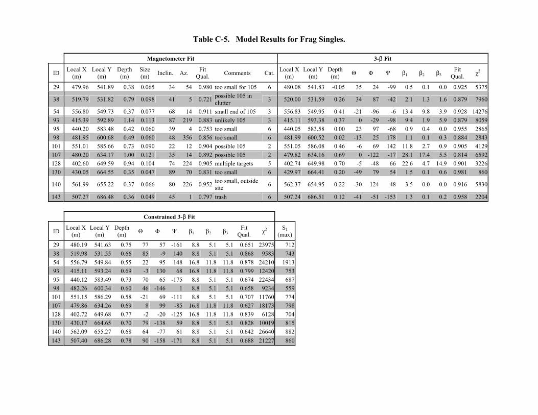
Table C-5. Model Results for Frag Singles.

Magnetometer Fit 3-$ Fit

ID Local X (m)

Local Y (m)

Depth (m)

Size (m) Inclin. Az. Fit

Qual. Comments Cat. Local X (m)

Local Y (m)

Depth (m) Θ Φ Ψ $1 $2 $3

Fit Qual. χ2

29 479.96 541.89 0.38 0.065 34 54 0.980 too small for 105 6 480.08 541.83 -0.05 35 24 -99 0.5 0.1 0.0 0.925 5375

38 519.79 531.82 0.79 0.098 41 5 0.721 possible 105 in clutter 3 520.00 531.59 0.26 34 87 -42 2.1 1.3 1.6 0.879 7960

54 556.80 549.73 0.37 0.077 68 14 0.911 small end of 105 3 556.83 549.95 0.41 -21 -96 -6 13.4 9.8 3.9 0.928 1427693 415.39 592.89 1.14 0.113 87 219 0.883 unlikely 105 3 415.11 593.38 0.37 0 -29 -98 9.4 1.9 5.9 0.879 805995 440.20 583.48 0.42 0.060 39 4 0.753 too small 6 440.05 583.58 0.00 23 97 -68 0.9 0.4 0.0 0.955 286598 481.95 600.68 0.49 0.060 48 356 0.856 too small 6 481.99 600.52 0.02 -13 25 178 1.1 0.1 0.3 0.884 2843

101 551.01 585.66 0.73 0.090 22 12 0.904 possible 105 2 551.05 586.08 0.46 -6 69 142 11.8 2.7 0.9 0.905 4129107 480.20 634.17 1.00 0.121 35 14 0.892 possible 105 2 479.82 634.16 0.69 0 -122 -17 28.1 17.4 5.5 0.814 6592128 402.60 649.59 0.94 0.104 74 224 0.905 multiple targets 5 402.74 649.98 0.70 -5 -48 66 22.6 4.7 14.9 0.901 3226130 430.05 664.55 0.35 0.047 89 70 0.831 too small 6 429.97 664.41 0.20 -49 79 54 1.5 0.1 0.6 0.981 860

140 561.99 655.22 0.37 0.066 80 226 0.952 too small, outside site 6 562.37 654.95 0.22 -30 124 48 3.5 0.0 0.0 0.916 5830

143 507.27 686.48 0.36 0.049 45 1 0.797 trash 6 507.24 686.51 0.12 -41 -51 -153 1.3 0.1 0.2 0.958 2204

Constrained 3-$ Fit

ID Local X (m)

Local Y (m)

Depth (m) Θ Φ Ψ $1 $2 $3

Fit Qual. χ2 S1

(max)

29 480.19 541.63 0.75 77 57 -161 8.8 5.1 5.1 0.651 23975 71238 519.98 531.55 0.66 85 -9 140 8.8 5.1 5.1 0.868 9583 74354 556.79 549.84 0.55 22 95 148 16.8 11.8 11.8 0.878 24210 191393 415.11 593.24 0.69 -3 130 68 16.8 11.8 11.8 0.799 12420 75395 440.12 583.49 0.73 70 65 -175 8.8 5.1 5.1 0.674 22434 68798 482.26 600.34 0.60 46 -146 1 8.8 5.1 5.1 0.658 9234 559

101 551.15 586.29 0.58 -21 69 -111 8.8 5.1 5.1 0.707 11760 774107 479.86 634.26 0.69 8 99 -85 16.8 11.8 11.8 0.627 18173 798128 402.72 649.68 0.77 -2 -20 -125 16.8 11.8 11.8 0.839 6128 704130 430.17 664.65 0.70 79 -138 59 8.8 5.1 5.1 0.828 10019 815140 562.09 655.27 0.68 64 -77 61 8.8 5.1 5.1 0.642 26640 882143 507.40 686.28 0.78 90 -158 -171 8.8 5.1 5.1 0.688 21227 860

Table C-6. Model Results for Clutter.

Magnetometer Fit 3-$ Fit

ID Local X (m)

Local Y (m)

Depth (m)

Size (m) Inclin. Az. Fit

Qual. Comments Cat. Local X (m)

Local Y (m)

Depth (m) Θ Φ Ψ $1 $2 $3

Fit Qual. χ2

47 541.64 534.72 0.96 0.158 73 306 0.845 155 or 8 in deep, large clutter on top 2 541.96 535.37 0.59 -8 33 82 52.8 15.7 36.2 0.894 49779

48 544.28 535.12 0.35 0.074 5 25 0.941 likely clutter 5 544.82 534.90 0.33 -7 95 -176 14.3 8.8 2.9 0.678 133241

90 431.30 595.78 0.37 0.095 14 43 0.919 shallow 105 1 431.34 595.81 0.08 12 49 97 4.2 0.7 1.4 0.973 5382

94 435.97 588.71 0.38 0.055 11 52 0.940 trash 6 436.09 588.58 0.03 7 24 25 1.1 0.2 0.0 0.915 2819

116 413.49 616.89 0.38 0.085 17 350 0.957 low end of 105mm 1 413.58 616.90 0.10 4 101 23 4.4 0.1 1.2 0.967 7980

168 523.52 700.80 0.33 0.084 24 30 0.936 possible shallow 105mm 2 523.50 700.83 0.06 -52 11 -96 3.7 1.1 2.5 0.984 9203

Constrained 3-$ Fit

ID Local X (m)

Local Y (m)

Depth (m) Θ Φ Ψ $1 $2 $3

Fit Qual. χ2 S1

(max)

47 542.11 535.43 0.62 13 29 -147 40.6 28.8 28.8 0.826 98513 3231

48 544.81 534.91 0.72 -5 112 -173 40.6 28.8 28.8 0.587 168772 2044

90 431.29 595.73 0.36 2 38 -40 8.8 5.1 5.1 0.758 52957 1770

94 436.05 588.54 0.65 8 19 134 8.8 5.1 5.1 0.412 19932 674

116 413.74 616.87 0.49 86 106 160 8.8 5.1 5.1 0.673 78485 1869

168 523.61 700.90 0.26 -63 -122 -151 8.8 5.1 5.1 0.955 26602 4058

ESTCP Program Office

901 North Stuart StreetSuite 303Arlington, Virginia 22203

(703) 696-2117 (Phone)(703) 696-2114 (Fax)

e-mail: estcp@estcp.orgwww.estcp.org