Estimates of Air Emissions from AsphaltStorage Tanks and Truck Loading

David C. TrumboreAsphalt Technology Laboratory. Owens Corning, Summit, IL 60501

Title V of the 1990 Clean Air Act requires the accurateestimation of emissionsprocesses, and places theburden

rom all U.S. manufacturing of proof for that estimate

on the process owner. This paper is published as a tool to assist in the estimation of air emissions from hot asphaltstorage tanks and asphalt truck Loading operations. Dataare presented on asphalt vapor pressure, vapor molecularweight, and the emission split between volatile organiccompounds and particulate emissions that can be usedwith AP-42 calculation techniques to estimate airemissions from asphalt storage tanks and truck loadingoperations. Since current AP-42 techniques are not validin asphalt tanks with active fume removal, a differenttechnique for estimation of air emissions in those tanks,based on direct measurement of vapor space combustiblegas content, is proposed. Likewise, since AP-42 does notaddress carbon monoxide or hydrogen sulfide emissionsthat are known to be present in asphalt operations, thispaper proposesFinally,

techniques for estimation of those emissions.data are presented on the effectiveness of fiber bed

jilters in reducing air emissions in asphalt operations.

INTRODUCTIONThe use of asphalt is prevalent throughout recorded

history. It is produced in refinery distillation towers andsolvent extraction units. Asphalt is modified by severalmeans: reacting with oxygen in blowing operations toproduce roofing asphalts, emulsifying to produce anaqueous liquid at ambient temperature, blending withsolvents to make asphalt cutback, or blending or evenreacting with polymers to make polymer modified asphalt.In all these cases the asphalt is stored in tanks, usuallyfixed roof tanks, and is loaded into trucks to ship tocustomers.

Title V of the 1990 Clean Air Act required the accurateestimation of emissions from all U.S. manufacturingprocesses, and placed the burden of proof for that estimateon the process owner. In response to Title V, OwensCorning analyzed options for estimating emissions from

250 Winter 1999

asphalt tanks and loading operations and this paper is theresult of that study. In particular, attempts have been madeto develop data to be used with existing calculationmethods to estimate air emissions in asphalt operations, todevelop calculation schemes that work when existingmethods cannot be used, and to expand the number ofpollutants estimated. The techniques described in thispaper have been used by Owens Corning to estimateasphalt emissions from their asphalt plants for many Title Vpermit applications.

Owens Corning also evaluated appropriate emissionfactors for the asphalt blowing process and that analysis hasbeen published [I].

The Emission Factor and Inventory Group in the U. S.Environmental Protection Agency’s (EPA) Office of AirQuality Planning and Standards develops and maintains adatabase of emission factors and a series of calculationmethods for estimating air emissions from manufacturingprocesses. These emission factors are published in a seriesknown as AP-42 [2]. One technique published in AP-42calculates hydrocarbon emissions from a fixed roof tankstoring petroleum products [3], and another calculatesemissions for loading trucks with petroleum products [4].These techniques require data on asphalt vapor pressureand the molecular weight of the -asphalt vapor. Thecalculations result in an estimate of the amount ofhydrocarbons emitted from the process. To complete theemission estimate, these hydrocarbons need to be split intoparticulate emissions (PM) and volatile organic compounds(VOC), and any control device collection or destructionefficiencies need to be applied.

In the AP-42 calculation of emissions from fixed rooftanks it is assumed that the motive force pushing vapor outof the tank comes from either the pumping of liquid intothe tank or the expansion of tank contents due totemperature changes. For tanks with an active ventilationsystem this assumption is invalid and a different method ofemission estimation is required. This is especially true if anair sweep is used to control the vapor space composition to

Environmental Progress (Vol.18, No.4)

No.4)

prevent explosive conditions [5,6]. A technique to estimateemissions from these actively controlled tanks is describedin the section of this paper on non AP-42 estimates.

AP-42 EMISSION ESTIMATING TECHNIQUES FOR ASPHALT EQUIPMENTPassive vented hot asphalt tanks: AP-42 for fixed roof

petroleum tanks can be used to calculate total hydrocarbonemissions from asphalt and oil tanks that are passivelyvented to the atmosphere. This AP-42 calculation, simplystated, determines the amount of hydrocarbon in the tankvapor space from the vapor pressure of the material in thetank at the liquid surface temperature, and then calculatesthe amount of vapor forced out of the tank due to liquidbeing actively pumped into the tank (working losses), ordue to thermal expansion or contraction of tank contentsdriven by ambient temperature changes (breathing losses).The result is an actual weight of hydrocarbon emissions ina specified time period. A detailed description of the tankcalculations is available from th e EPA web site [3]. The AP-42 calculation requires a vapor pressure versus temperaturecurve for the asphalt, and also estimates of the vapor phasemolecular weight and partition of hydrocarbons into VOC and particulate, in addition to process data like asphaltthroughput. temperature. and tank level. If the tankpassively breathes through a control device, then theappropriate control efficiency is applied to the VOC andparticulate emissions calculated from AP-42.

Hot Asphalt Loading: The AP-42 calculation forhydrocarbon emissions from truck or rail tank car loadingof asphalt is done by estimating the amount of evaporationduring the loading process. The estimate takes into accountthe turbulence and vapor liquid contact induced by themethod of loading, i.e . submerged versus splash loading.The calculation result is an emission related to the numberof tons of material loaded into the truck. Vapor pressureversus temperature c urve s, , temperature of loading, andthroughputs are key variables in this calculation. Again, thehydrocarbon emission resulting from this calculation needsto be split into pa rticu la tes s and VOCs and control devicecollection and destruction efficiencies need to be applied. Adetailed description of the loading calculations is availablefrom the EPA web site [4].

DATA NEEDED FOR APPLICATION OF AP-42 TO ASPHALT EQUIPMENTVapor Pressure: Information on asphalt vapor pressure as a

function of temperature is not readily available in theliterature and its measurement is not common. However,these data are essential to use AP-42 calculations forestimating asphalt tank and loading emissions. Asphaltsfrom different crude oil sources and from differentprocesses will differ in composition and vapor pressure. Inthe extreme, every residual material used in asphaltprocessing would need to be measured for vapor pressureat multiple temperatures. This would entail a prohibitive

estimates. To provide a cost effective solution to thisproblem for its emission calculations, Owens Corning has

Environmental Progress (Vol. 18 , No.4)

characterized the vapor pressure of three basic classes ofasphalt materials. chosen by their processing history. Anestimate of the vapor pressure of each asphalt class wasmade by measuring asphalts from multiple crude oilsource s in each class and using the average vapor pressureat each temperature in a regression to generate one vaporpressure equation for tha t class. The three classes of asphaltchosen for this analysis follow.

Flux asphalts. or vacuum tower bottoms that can bein the asphalt blowing process to make

specification roofing asphalts. These materials generallyhave a higher vapor pressure than paving asphalts.Paving asphalts, or vacuum tower bottoms that meetpaving specifications.Oxidized asphalt, or vacuum tower bottoms that havebeen reacted with oxygen in the asphalt blowing processto increase their softening point and viscosity. Typicalsoftening points are greater than 19 0°F (88°C) Thesematerials are also called air blown asphalts and are usedextensively in the roofing industry. They generally havelower vapor pressure than the other two classes.

Va por pressure measurements described in this paper wereclone by the Phoenix Chemical Lab in Chicago using theIsoteniscope (ASTM D2879).

To facilitate computer calculations it is desirable to developan equation that accurately describes the relationship of vaporpressure and temperature. Thermodynamic treatment of thedependence of vapor pressure on temperature has led to theClausius modification of the Clapeyron equation [7].

Clausius Clapeyron Treatment of Vapor Pressure Data

In P = a + b/T

Where: P is the equilibrium vapor pressureof the liquid in question,a & b are constants. andT is the absolute temperature of the liquidin question.Values of a & b depend on the choice ofpressure and temperature units.

Table 1 and Figure 1 give an example of the agreement ofthis equation with vapor pressure data for oxidized asphaltsfrom 13 sources around the country. In Figure 1 , vaporpressure of each asphalt is plotted versus temperature to show

each individual asphalt’s data to the Clausius Clapeyronrela tionship .. The correlation coefficients in Table 1 indicatethat the agreement of this equation to all individual asphaltvapor pressure ve rsus temperature data is excellent, withcorrelation coefficients for the individual asphalts greater than0.9999. The agreement is also excellent for the individualasphalts making up the other two asphalt classes. Table 1 also presents the methodology to choose constants to use with the

Winter 19 99 251

amount of testing for minimal gain in accuracy of emission

the differences between asphalt's data to the Clausius Clapeyron

used

Table l.Vapor Pressure Data for Oxidized Asphalts

Temperature (°F1) All Data in mm Hg2

200 250 350 400 450 500 600 r value3

Plant A 0.39 2 7.9 26 77 550Plant C 0.42 2 7.9 26 670

H 0.43 2 7.7 25z: 180

165 410 590Plant I 0.44 1.9 7.2 22 59 140 340 680PlantK 0.43 1.7 6.1 18.5 50 115 205 510 680PlantM 0.28 1.2 4.6 15 41 97 210 640PlantN 0.19 0.88 3.5 12 34 85 190 430 590PlantP 0.46 1.8 6 44 96 195 410 710Plant0 0.11 0.47 1.7 13.2 34 74 142Plant J 0.16 0.64 2.2 6.2 14.8 36 72 135PlantS 0.28 1.05 3.3 9.4 23 50 105 200 350PlantS 0.28 1 3.2 10 25 58PlantX 0.1 0.4 1.5 4.7 12.5 33 75 152Class Standard 0.22 0.91 3.2 9.5 24.9 58.8 127 254 351 477Average 0.33 0.75 2.6 7.9 22.3 54.7 122 284 634 347

13459 b in Clausius Clapeyron curve for average vapor pressure data

1. 1 °C = (°F - 32) * 5/9 2. 1 Pa = 0.0075 mm Hg

the r value is for the fit of the vapor pressure data to the Clausius Clapeyron Equation

-0.999922929-0.999934558-0.999939281-0.999945804-0.999660554-0.999948167-0.999965421-0.999948079-0.999916578-0.999838114-0.999986213-0.999875798-0.999930649

-0.994026635

1000

100

FIGURE 1.Oxidized Asphalt Vapor Pressure Data in Clausius Clapeyron Format

9 10 11 12 13 14 16

Asphalt 300 550 575

225400

460

5.217.5

Plant

Vp

18.86 a in Clausius Clapeyron curve for average vapor pressure data

10,000 * 1/T (°R)215

0.1

Environmental Progress (Vol.18, No.4)252 Winter 1999

I I

II

A Plant A tI w-e I I

I I II I

A Plant H0 Plant Ix Plant K0 Plant M+ Plant N- Plant P- Plant 0l Plant Jm Plant S

1

0.1

2. 1 ° C = (° F-32)*5/9I / II AI .

Temperature (°F2)

1000

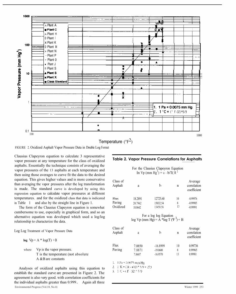
FIGURE 2. Oxidized Asphalt Vapor Pressure Data in Double Log Format

Clausius Clapeyron equation to calculate 3 representativevapor pressure at any temperature for the class of oxidizedasphalts. Essentially the technique consists of averaging thevapor pressures of the 13 asphalts at each temperature andthen using those averages to curve fit the data to the desiredequation. This gives higher values and is more conservativethan averaging the vapor pressures after the log transformationis made. The standard curve is developed by using thisregression equation to calculate vapor pressures at differenttemperatures. and for the oxidized class that data is indicated

in Table 1 and also by the straight line in Figure 1.The form of the Clausius Clapeyron equation is somewhat

cumbersome to use, especially in graphical form, and so analternative equation was developed which used a log/logrelationship to characterize the data.

Log Log Treatment of Vapor Pressure Data

log Vp = A * log(T) + B

Vp is the vapor pressure.T is the temperature (not absoluteA & B are constants

Analyses of oxidized asphalts using this equation toestablish the standard curve are presented in Figure 2. Theagreement is also very good. w ith correlation coefficients forthe individual asphalts greater than 0.999. Again all three

Class ofAsphalt a

Averagen correlation

coefficient

FluxPavingOxidized

18.2891 12725.60 10 -0.9997620.7962 15032.54 8 -0.9998518.8642 -0.99991

For a log log Equationlog Vp (mm Hg) = A * log T (°F 3) + B

Class ofAsphalt a

Averagen correlation

coefficient

Flux 7.0850 -16.8999 10 0.99736Paving 7.8871 -19.0600 8 0.99965Oxidized 7.0607 -16.9570 13 0.99981

Table 2. Vapor Pressure Correlations for Asphalts

For the Clausius Clapeyron EquationIn Vp (mm Hg1) = a - b/T( R 2

Environmental Progress (Vol.18, No.4) Winter 1999 253

13458.56 13

where

100

5

5

classes of asphalts show similar agreement, Pressure Summary: Table 2 gives a summary of the

regression constants to be used in either of the equationsdiscussed above to calculate the vapor pressure for the threeclasses of asphalt at any temperature. Also indicated are thenumber of asphalts that were used to develop the equationfor each class. and the average correlation coefficientcharacterizing the agreement of the data to the form of theequation for each individual asphalt in the class.

In AP-42 for tanks, the correct temperature to use in theTable 2 equations is the asphalt surface temperature in thetank. Since the surface temperature is rarely. if ever, knownwith certainty, the bulk temperature should be used toestimate emissions. In a well mixed tank the bulktemperature will be a good approximation of the surfacetemperature. Where mixing is not effective the surface will belower in temperature than the bulk and the use of the bulktemperature will give a conservative estimate of emissions. In

for loading trucks, the bulk temperature of the tankfrom which material is being loaded provides a good estimateof the actual loading temperature.

Asphalt Vapor Molecular Weight: Asphalt vapor molecularweight was determined by separation and analysis of theorganic species in the vapor spaces of 12 tanks storingdifferent types of asphalt. These profiles were obtained bydrawing known volumes of the tank vapor space through acharcoal tube, sealing and freezing the tube to limit loss ofthe sample, and then desorbing the organic material from thecharcoal with carbon disulfide and analyzing with gaschromatography using packed columns and flame ionizationdetectors. Analyses were performed by CHEMIR Laboratoryin St. Louis. Quantitative standards were used to identify theamount of individual normal alkanes from n-pentane to n-pentadecane. Peaks eluting between the normal alkanes wereassumed to he isomers of the hordering alkanes, especiallycyclic isomers of the lower carbon number alkane, andbranched or unsaturated isomers of the higher carbonnumber alkane. The molecular weights for the n-alkanespecies and molecular weight estimates for the intermediatespecies were used with the amount of that material measuredto calculate a weighted average vapor molecular weight foreach tank, and then the twelve tanks were averaged togetherto get the molecular weight used for hot asphalt vapors in theAP-42 calculations. The result was a molecular weight of 84,which is used with all three classes of asphalts. This analysisis detailed in Table 3. Not enough data were available toassign different values to the three asphalt classes,however, from the table the unblown flux material in twotanks gave molecular weights which bracketed theaverage. as did the two paving blend stocks.

This analysis gave a lower molecular weight for thevapor space of asphalt tanks than for several petroleumsolvents and fuel oils. This seems like a contradictionconsidering the nature of asphalt as the residuum materialcollected upon distillation. This contradiction is resolvedby considering that asphalt is not a uniform materialchemically and that the lower molecular weight materials

AP-42

Vapor

Environmental Progress (Vol.18, No.4)254 Winter 1999

Table 4. PM/VOC Partition Data fromOwens Corning Testing

AsphaltPlant 0

Tank A Tank B Tank c

VOC Test 0.73PM Test 0.21VOC Fraction 0.78

1.16 0.980.38 0.300.75 0.77

lb/hr1

lb/hr

Koofing Plant S Coater Results:Measured at different points. Data indicated 22% of total

emission (VOC + PM) was PM and 78% was VOC

1. 1 kg/sec = 0.0076 * lb/hr

are preferentially evaporated More importantly. it has alsobeen established that thermal cracking of asphalt in hotstorage tanks creates low molecular weight materials whichaccumulate in the tank vapor spaces [5,6].

Asphalt Liquid Molecular Weight: The actual bulk asphaltmolecular weight is not needed for AP-42 calculations ofemissions from tanks or loading racks. but is useful in somecalculations that are beyond the scope of this paper, forexample using Raoult's law for crude estimates of emissionsfrom mixtures of asphalt and other materials. Molecularweight of bulk asphalt is not a well defined materialproperty, both because asphalt is such a complex mixtureand because intermolecular interactions in the asphaltcreate the appearance of high molecular weight in manymeasurement techniques. The measured molecular weightis usually not truly representative of the covalently bondedmolecules, The difficulty in getting accurate asphaltmolecular weight measurements is extensively discussed inthe literature [8, 9, 10]. The use of Gel PermeationChromatography[8], Field-Ionization Mass Spectrometry [8].Vapor Pressure Osmometry [8,9,10], and Freezing PointDepression [10] have all been evaluated as methods formeasuring the molecular weight of asphalt or itscomponents. The topic is further complicated for emissioncalculations by the fact that many of the measurementshave been made on fractions of the asphalt and not on theneat asphalt. In general. for very rough estimates, a valueof 1000 [8] can be used for the molecular weight of bulkasphalt. This value should be used with the understandingthat there is much variation in the true molecular weightand in the tendency for intermolecular interaction due topetroleum crude source and processing conditions.

Partition of hydrocarbon emissions that are particulate and VOC:Because of its heterogeneous nature, asphalt fumes arevaried and may have components that are classified ascondensed particulates (PM) or as volatile organiccompounds (VOCs). It m-as evident in analyzing asphaltfume results that the difference between these two classesof criteria pollutants is really defined by the method used to

test for the pollutants. Estimation schemes described in thispaper calculate the sum of both (AP-42) or just the VOCcomponent (non-AP-42 technique described below), andthe partition needs to be understood to provide the bestestimated values of the two pollutants. To that end. testshave been done on both asphalt tank exhausts in anOwens Corning asphalt plant and on the asphalt shinglecoater exhausts in an Owens Corning roofing plant usingEPA Methods 5 & 25A sampling protocols which defineVOC and PM emissions in hydrocarbon fumes. Underconditions specified by the test method some fraction ofthe fume is captured on a filter and this is defined as aparticulate emission, while a fraction of the hydrocarbonemission passes through the filter and this is defined as aVOC emission. The results of the split in the totalhydrocarbon fume between VOC and particulate wereapproximately 78% VOC and 22% particulate in the asphaltequipment. in spite of the basic difference between ashingle coater and a storage tank. Data from these tests aregiven in Table 4.

NON AP-42 CALCULATIONS TECHNIQUES:Estimation of VOC and particulate emissions from tanks with

fume control: Many asphalt tanks have their fumes activelycollected and treated in a control device, either a fiber bedfilter or an incinerator. In these tanks it is common atOwens Corning to allow some air to pass through the tankvapor spaces to create an air sweep that controlscombustible fumes well below the lower explosion limit(LEL) in order to prevent explosions. Because of the activeremoval of fumes in these systems, and the bleeding of airinto the vapor space. the assumptions underlying the AP-42tank calculations no longer apply. Specifically the drivingforce for the flow of fumes out of the tank is no longer justthe working and breathing losses. and an alternativemethod of emission calculation is needed.

Several years ago safety concerns with asphalt tanksprompted Owens Corning to institute the periodicmeasurement of the combustible gas concentration in allasphalt tank vapor spaces [5]. With the advent of Title V itwas recognized that these measurements could be used toestimate VOC emissions. As part of the safety program.techniques were developed to make this routinemeasurement simple and easy. and the result was the useof Mine Safety Appliance (MSA) combustion meters toquantify the hydrocarbon concentration in terms of thefraction (or %) of the LEL. This technique and the validationof its accuracy has been described in detail in a separatepublication [6]. In addition to the combustible gasmeasurement, a slightly more complicated technique is alsodescribed and validated that gives the concentration ofethane, methane. and other light combustible gasesseparate from propane and larger hydrocarbons. Thistechnique involves using a charcoal tube in the linebetween the tank and the MSA meter. The charcoal tubeadsorbs all propane and higher hydrocarbons [6], with theresultant reading at the MSA meter due only to the lighter

Environmental Progress (Vol.18, No.4) Winter 1999 255

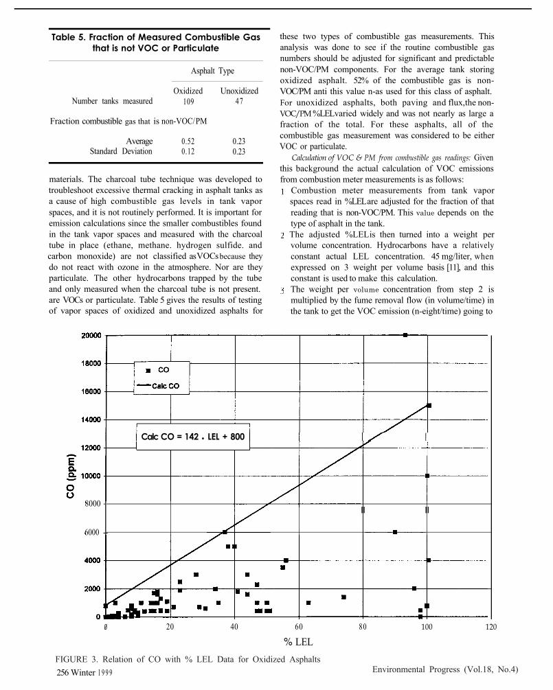
Table 5. Fraction of Measured Combustible Gasthat is not VOC or Particulate

Asphalt Type

Number tanks measuredOxidized Unoxidized

109 47

Fraction combustible gas that is non-VOC/PM

Average 0.52 0.23Standard Deviation 0.12 0.23

materials. The charcoal tube technique was developed totroubleshoot excessive thermal cracking in asphalt tanks asa cause of high combustible gas levels in tank vaporspaces, and it is not routinely performed. It is important foremission calculations since the smaller combustibles foundin the tank vapor spaces and measured with the charcoaltube in place (ethane, methane. hydrogen sulfide. andcarbon monoxide) are not classified asVOCs because theydo not react with ozone in the atmosphere. Nor are theyparticulate. The other hydrocarbons trapped by the tubeand only measured when the charcoal tube is not present.are VOCs or particulate. Table 5 gives the results of testingof vapor spaces of oxidized and unoxidized asphalts for

these two types of combustible gas measurements. Thisanalysis was done to see if the routine combustible gasnumbers should be adjusted for significant and predictablenon-VOC/PM components. For the average tank storingoxidized asphalt. 52% of the combustible gas is non-VOC/PM anti this value n-as used for this class of asphalt.For unoxidized asphalts, both paving and flux,the non-VOC/PM % LEL varied widely and was not nearly as large afraction of the total. For these asphalts, all of thecombustible gas measurement was considered to be eitherVOC or particulate.

Calculation of VOC & PM from combustible gas readings: Giventhis background the actual calculation of VOC emissionsfrom combustion meter measurements is as follows:

Combustion meter measurements from tank vaporspaces read in %LEL are adjusted for the fraction of thatreading that is non-VOC/PM. This value depends on thetype of asphalt in the tank.The adjusted %LEL is then turned into a weight pervolume concentration. Hydrocarbons have a relativelyconstant actual LEL concentration. 45 mg/liter, whenexpressed on 3 weight per volume basis [11], and thisconstant is used to make this calculation.The weight per volume concentration from step 2 ismultiplied by the fume removal flow (in volume/time) inthe tank to get the VOC emission (n-eight/time) going to

Calc CO = 142 l LEL + 800

8000 -II II

6000 --

0 20 40 60 80 100 120

% LEL

256

Winter 1 9 9 9

FIGURE 3. Relation of CO with % LEL Data for Oxidized AsphaltsEnvironmental Progress (Vol.18, No.4)

2500

2000

1500

1000

500

0

I

I

I I

0 20 40 60 80 100 120

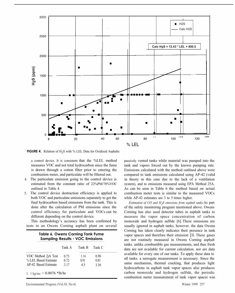
% LELFIGURE 4. Relation of H2S with % LEL Data for Oxidized Asphalts

a control device. It is consistent that the %LEL methodmeasures VOC and not total hydrocarbon since the fumeis drawn through a cotton filter prior to entering thecombustion meter, and particulate will be filtered out.

The particulate emission going to the control device isestimated from the constant ratio of 22%PM/78%VOC outlined in Table 4.

The control device destruction efficiency is applied toboth VOC and particulate emissions separately to get thefinal hydrocarbon based emissions from the tank. This isdone after the calculation of PM emissions since thecontrol efficiency for particulate and VOCs can bedifferent depending on the control device.This methodology’s accuracy has been confirmed by

tests in an Owens Corning asphalt plant on several

Table 6. Owens Corning Tank FumeSampling Results - VOC Emissions

Tank A Tank B Tank C

VOC Method 2jA Test 0.73 1.16 0.98 LEL Based Estimate 0.72 0.91 0.83

AP-42 Based Estimate 3.17 4.5 3.39

= 0.0076 *lb/hr

passively vented tanks while material was pumped into thetank and vapors forced out by the known pumping rate.Emissions calculated with the method outlined above werecompared to tank emissions calculated using AP-42 (validin theory in this case due to the lack of a ventilationsystem), and to emissions measured using EPA Method 25A.As can be seen in Table 6 the method based on actualcombustion meter tests is similar to the measured VOCswhile AP-42 estimates are 3 to 5 times higher.

Estimation of CO and H2S emissions from asphalt tanks: As partof the safety monitoring program mentioned above. OwensCorning has also used detector tubes in asphalt tanks tomeasure the vapor space concentration of carbonmonoxide and hydrogen sulfide [6]. These emissions areusually ignored in asphalt tanks, however. the data OwensCorning has taken clearly indicates their presence in tankvapor spaces and therefore their emission [il. These gasesare not routinely measured in Owens Corning asphalttanks. unlike combustible gas measurements, and thus freshdata are not available for current calculation. nor are dataavailable for every one of our tanks. To apply these data toall tanks. a surrogate measurement is necessary. Since thesame mechanism, thermal cracking, that produces lighthydrocarbons in asphalt tank vapor spaces also producescarbon monoxide and hydrogen sulfide, the periodiccombustion meter measurement of tank vapor spaces was

4.

5.

%

1. 1 kg/sec

H2S

(p

pm

)

3000

H2S

Calc H2S

Calc H2S = 12.43 * LEL + 400.5

Environmental Progress (Vol.18, No.4) Winter 1999 257

Table 7. Asphalt Plant 0:Tank Emissions of H2S and CO

Tank A Tank B Tank C

DataActual Test

% LEL based estimate0.06 0.12 0.15 lb/hr1

0.19 0.18 0.20 lb/hr

CO DataActual Test

% LEL based estimate0.20 0.17 0.23 lb/hr0.74 0.85 0.83

1. 1 kg/sec = 0.0076 * lb/hr

investigated as a surrogate for CO and Data for COand are plotted in Figures 3 and 4. Because of thescatter of data in the correlations a representative line waschosen for each material that was more conservative thannearly all of the data, in other words a line that defined amaximum concentration of CO and that could beexpected in an asphalt tank from the combustion metermeasurement. The equations used in the calculation of COand concentrations from combustion meter results

CO (ppm) = 142 *%LEL + 800 for oxidized asphalt = 12.43 *%LEL + 400.5 for oxidized asphalt

In unoxidized asphalt no such correlation was seen and values of 500 ppm are used for both species.

To estimate an emission from this correlation the CO and concentrations are multiplied by the flow out of the tank

to get emissions. and conversion factors are used to transformthis into a weight per time emission. Any control devicedestruction efficiency is then applied. The emissions usingthese techniques can be significant. Limited directmeasurement in an Owens Corning asphalt plant wasconsistent with this approach. at least in so far as that the

approach was conservative. was the closer of thetwo estimates. Data are presented in Table 7.

One consequence of fume incineration is that one mole of in the fumes is oxidized to one mole of The amount

of oxidized to SO, is the amount of generated minusboth the amount that escapes at the source and the amountthat is not incinerated at the control device. or in effect thetotal uncontrolled H2S emissions minus the emissions

g after control. Because of the reaction with oxygenand the molecular weight differences between H2S and SO2,every pound (2.2 kg) of H2S emission is oxidized to 1.88pounds (4.14 kg) of SO2 emission.

LoadingRack emissions of CO and H2S: As in the tanks. %LELversus CO and H2S correlations are used to estimate thesecomponents in loading rack emissions. Again, withincineration, the H2S is oxidized to SO2. Flow out of thetank truck during loading is needed for CO and H2S calculations. When fumes are collected, that flow can be

either the more conservative flow induced by the fume fan, or the lower and more realistic displacement of air by theasphalt being loaded. When no collection takes place thatflow is the displacement of air by asphalt being loaded.Combustion meter measurements of %LELs from the tanks

for loading are used for these calculations.

EFFECTIVENESS OF FIBER BED FILTERS FOR ASPHALT FUME EMISSIONCONTROL

One device used extensively to control asphalt fumes isa fiber bed filter. Fumes are actively pulled through thesefilters or passively hreathe through these filters. Their firstuse at Owens Corning was to control opacity to comply

NSPS regulations, and for this application they haveproven to he quite effective.

Testing was done on both asphalt tanks and on aroofing line center to determine the control efficiency offiber bed filters for both VOC and particulate emissions.Data from the testing are summarized in Table 8. In allcases. the particulate collection in the filter exceeded 90%of the emissions in the input stream. This value agrees well

manufacturer’s estimate of 95% and with theobservation that these devices can eliminate opacity.However, VOC removal varied widely in the tests. With theaverage removal near zero, and a very large variation, it

decided that no removal of VOC by these filters could assumed. Although organic oil is collected. this oil is

considered part of the particulate fraction of thehydrocarbons in the fumes and not the VOC fraction.Indeed the lack of removal of VOCs by these filters isconsistent with the method of partitioning hydrocarbonsinto VOC and particulate described above -- namely VOCspass through a testing filter and particulate do not. Basedon the effectiveness of these control devices to eliminateopacity it is assumed that particulate greater than 10 micronis captured by the fiber bed filter so that the totalparticulate emissions from the fiber bed filter are

to be PM10 emissions.Fiber bed filters are not considered to he a control

device for CO and H2S in tank or loading rack fumestreams.

Table 8. Effectiveness of Fiber Bed Filtersfor Emission Control from Asphalt Tanks

Equipment Pollutant Control Efficiency

0 Tank 1

Tank 57

Tank 1

Asphalt 0 0 Tank 1 0 57

Roofing I Coater

0Asphalt 0Asphalt 0Asphalt 0

Tank 1 Total ParticulateTank 57 Total Particulate 90.7%

Tank 1 Filterable Particulate 100.0% Filterable 100.0%

H2S

lb/br

with

used

was

with

considered

be

Plant

Asphalt

AsphaltAsphalt

Asphalt

Tank

VOCVOCVOCVOCVOC

-35.7%5.7%

43.4% 5.3% 0.0%

95.7%

remaining

H2S

H2S

H2S

H2S

H2SH2S

H2S

H2S

H2S

H2S SO2

%LEL

conservative

(ppm)

258 Winter 1999 Environmental Progress (Vol.18, No.4)

Table 9. Summary of Data for Calculating Asphalt Tank Emissions

Data Type Flux Asphalt Paving Asphalt Oxidized Asphalt

Clausius Clapeyron constant a for vapor pressure 1 18.2891 20.7962 18.8642Clausius Clapeyron constant b for vapor pressure 1 12725.6 15032.54 13458.56Log Log constant A for vapor pressure 2 7.085 7.8871 7.0607Log Log constant B for vapor pressure 2 -16.8999 -19.06 -16.957Asphalt vapor molecular weight use 84 for all types of asphaltAsphalt liquid molecular weight very rough estimate - 1000Partition of hydrocarbon fumes into particulate and VOC use 22% particulate, 78% VOC for all types% fumes that are VOC or particulate, versus non VOC/PM100% 100% 48%Vapor space carbon monoxide (conservative estimate)ppm500 500 142* % LEL + 800Vapor space hydrogen sulfide (conservative estimate) ppm500 500 12.43*%LEL + 400.5Fiber bed filter control of VOC use 0% for all asphalt typesFibe4r bed filter control of particulate use 90% for all asphalt types

1.In Vp(mm Hg) = a + b/T( °R) 1 Pa = 0.0075mm Hg, 1 °K = (°R-492)*5/9 +2732.log Vp (mm Hg) = A*log T( °F) + B1 °C = (°F - 32)* 5/9

CONCLUSIONS Estimation of air emissions for asphalt tanks and loadingracks can be done using AP-42 calculation methods given appropriate data on asphalt properties. More preciseestimates of emissions, or estimates for tanks usingventilation schemes that compromise the AP-42assumptions, can be done using a simple measurement ofthe combustible gas in the vapor space. Methods to do thisare outlined in the paper. Data that is useful with all thesemethods are summarized in Table 9. These data are givenfor three major classes of asphalt: paving, flux andoxidized

LITERATURE CITED1. Trumbore, D.C., "The magnitude and source of air emissions from asphalt blowing operations," Environmental Progress,17, (1), pp. 53-59 (Spring 1998).2. U.S.Environmental Protection Agency, "Introduction to 5th edition of AP-42 Emission Factors," U. S. EPA, January,1995,from the Internet at http://www.epa.gov/ ttn/chief/ap42.html (accessed May 14, 1998). 3. U.S Environmental Protection Agency, Chapter 7.1 of the 5th edition of AP-42 Emission Factors, U.S.EPA, "Organic Liquid Storage Tanks," September, 1997, from the Internet at http://www.epa.gov/ttn/chief/ap42.html (accessed May 14, 1998).4. U.S.Envoironmental Protection Agency, Chapter 5.2 of the

5th edition of AP-42 Emission Factors, U.S. EPA,"Transportation and Marketing of Petroleum Liquids,"January, 1995, from the Internet at http://www.epa.gov/ttn/chief/ap42.html (accessed May 14, 1998).

5. Trumbore, D.C. and C.R.Wilkinson, "Better understanding needed for asphalt tank-explosion hazards," Oil Gas J., 87, pp.38-41 (September 18, 1989).6. Trumbore, D.C., C.R.Wilkinson, and S.Wolfersberger, "Evaluation of techniques for in situ determination of explosion hazards in asphalt tanks," J.Loss Prev. Process Ind., 4, pp. 230-235 (July,1991).7. Schmidt, A.X. and H.L. List, "Material and Energy Balance," Prentice Hall, Inc., Englewood Cliffs, New Jersey, pp. 40-41 (1962).8. Boduszynski, M.M., "Asphaltenes in petroleum Asphalt: Composition and Formation," Chapter 7, in "The Chemistry of Asphaltenes," American Chemical Society, Washington, D.C., pp. 119-135 (1981).9. Storm, D.A., et al., "Upper bound on number average molecular weight of asphaltenes," Fuel, 69, pp. 735-738 (June, 1990).10. Speight, J.G., and S.E.Moschopedis, "Asphaltene molecular weights by a cryoscopic method," Fuel, 56, pp 344-345 (July, 1977).11. Bodurtha, F.T., "Industrial Explosion Prevention and Protection," McGraw Hill, Inc, New york, New York, page 11 (1980).

Environmental Progress (Vol.18, No.4) Winter 1999 259