Estimates of heat kernels on Riemannian manifolds

Alexander Grigor’yanImperial College

London SW7 2BZEngland

email: a.grigoryan@ic.ac.ukURL: www.ma.ic.ac.uk/˜grigor

May 1999

Contents

1 Introduction 2

2 Construction of the heat kernel on manifolds 32.1 Laplace operator . . . . . . . . . . . . . . . . . . . . . . . . . . . . . . . . . . . . 32.2 Eigenvalues and eigenfunctions of the Laplace operator . . . . . . . . . . . . . . . 42.3 Heat kernel in precompact regions . . . . . . . . . . . . . . . . . . . . . . . . . . 52.4 Maximum principle and positivity of the heat kernel . . . . . . . . . . . . . . . . 72.5 Heat semigroup on a manifold . . . . . . . . . . . . . . . . . . . . . . . . . . . . . 9

3 Integral estimates of the heat kernel 103.1 Integral maximum principle . . . . . . . . . . . . . . . . . . . . . . . . . . . . . . 103.2 The Davies inequality . . . . . . . . . . . . . . . . . . . . . . . . . . . . . . . . . 113.3 Stochastic completeness . . . . . . . . . . . . . . . . . . . . . . . . . . . . . . . . 14

4 Eigenvalues estimates 15

5 Pointwise estimates of the heat kernel 185.1 Gaussian upper bounds for the heat kernel . . . . . . . . . . . . . . . . . . . . . . 185.2 Mean-value property . . . . . . . . . . . . . . . . . . . . . . . . . . . . . . . . . . 225.3 On-diagonal lower bounds and the volume growth . . . . . . . . . . . . . . . . . 25

6 On-diagonal upper bounds and Faber-Krahn inequalities 296.1 Polynomial decay of the heat kernel . . . . . . . . . . . . . . . . . . . . . . . . . 296.2 Arbitrary decay of the heat kernel . . . . . . . . . . . . . . . . . . . . . . . . . . 316.3 Localized upper estimate . . . . . . . . . . . . . . . . . . . . . . . . . . . . . . . . 376.4 Relative Faber-Krahn inequality and the decay of the heat kernel as V (x,

√t)−1. 38

7 Isoperimetric inequalities 407.1 Isoperimetric inequalities and λ1(Ω) . . . . . . . . . . . . . . . . . . . . . . . . . 407.2 Isoperimetric inequalities and the distance function . . . . . . . . . . . . . . . . . 417.3 Minimal submanifolds . . . . . . . . . . . . . . . . . . . . . . . . . . . . . . . . . 427.4 Cartan-Hadamard manifolds . . . . . . . . . . . . . . . . . . . . . . . . . . . . . . 427.5 Manifolds of bounded geometry . . . . . . . . . . . . . . . . . . . . . . . . . . . . 457.6 Covering manifolds . . . . . . . . . . . . . . . . . . . . . . . . . . . . . . . . . . . 497.7 Spherically symmetric manifolds . . . . . . . . . . . . . . . . . . . . . . . . . . . 517.8 Manifolds of non-negative Ricci curvature . . . . . . . . . . . . . . . . . . . . . . 52

1

1 Introduction

The purpose of these notes is to give introduction to the subject of heat kernels on non-compactRiemannian manifolds. By definition, the heat kernel for the Euclidean space Rn is the (unique)positive solution of the following Cauchy problem in (0,+∞) × Rn

∂u∂t = ∆u ,u(0, x) = δ(x− y),

where u = u(t, x) and y ∈ Rn. It is denoted by p(t, x, y) and is given by the classical formula

p(t, x, y) =1

(4πt)n/2exp

(−|x− y|2

4t

). (1.1)

In other words, p(t, x, y) is a positive fundamental solution to the heat equation ∂u∂t = ∆u . This

means, in particular, that the Cauchy problem∂u∂t = ∆u,u(0, t) = f(x)

is solved by

u(t, x) =∫

Rn

p(t, x, y)f(y)dy,

provided f is a bounded continuous function.Another definition of the heat kernel (which justifies the letter p) is as follows: it is the

transition density of the Brownian motion in Rn (up to the change of time t → t/2). Giventhat much, it is not surprising that the heat kernel plays a central role in potential theory inRn.

Consider now an arbitrary smooth connected Riemannian manifold M . There is a naturalgeneralization of the Laplace operator linked to the Riemannian structure of M . It is calledthe Riemannian Laplace operator or the Laplace-Beltrami operator and is also denoted by ∆.It turns out that the notion of the heat kernel can be defined on any manifold. Let us denote italso by p(t, x, y), where t > 0 and x, y ∈M . However, explicit formulas for p(t, x, y) exist onlyfor a few classes of manifolds possessing enough symmetries. The simplest explicit heat kernelformula after (1.1) is one for the three-dimensional hyperbolic space H3 which reads as follows

p(t, x, y) =1

(4πt)3/2exp

(−d

2

4t− t

)d

sinh d, (1.2)

where d = d(x, y) is the geodesic distance between x, y ∈ H3. Clearly, there is certain similaritybetween (1.1) and (1.2) (note that |x− y| is the geodesic distance in Rn) but there are alsotwo distinctions: the terms exp(−t) and d

sinhd in (1.2). They reflect the difference between thegeometries of the Euclidean and hyperbolic spaces.

It turns out that the heat kernel is rather sensitive to the geometry of manifolds, whichmakes the study of the heat kernel interesting and rich from the geometric point of view. Onthe other hand, there are the properties of the heat kernel which little depend on the geometryand reflect rather structure of the heat equation. For example, the presence of the Gaussianexponential term exp

(− d2

4t

)in the heat kernel estimates is one of such features.

Most part of these notes is devoted to the heat kernel upper estimates on arbitrary manifolds.We discuss both general techniques of obtaining the heat kernel bounds, presented in Sections3, 5, 6, and their applications for particular classes of manifolds, in Section 7. In Section 4,we apply the heat kernel bounds to estimate eigenvalues of the Laplace operator. Many resultsare supplied with proofs whose purpose is to demonstrate the underlying ideas rather than toachieve the full generality.

2

We do not aim at a detailed account of lower estimates of the heat kernel and touch only oneaspect of those in Section 5.3, not the least because this subject is so far not well understood.Other results on the lower bounds of heat kernel on manifolds can be found in [15], [28], [67],[78], [98], [110], [120], [123].

We have to skip some other interesting questions related to the heat kernels such as the Har-nack inequality [67], [68], [98], [120], [121], comparison theorems [28], [52], short time asymp-totics [62], [85], [105], [112], [119], [131], estimates of time derivatives of the heat kernel [44],[49], [71], gradient estimates [82], [86], [98], [100], [125], [117], [138], [141], discretization tech-niques [24], [25], [34], [88], homogenization techniques [2], [11], [90], [110], etc. Finally, we donot treat heat kernels on underlying spaces other than Riemannian manifolds and for operatorsother than the Laplace operator. See the following references for heat kernels

- on symmetric spaces [3];

- on groups and Lie groups [1], [13], [14], [108], [118], [135];

- for random walks on graphs [30], [53], [79], [83], [89], [114], [136];

- for second order elliptic operators with lower order terms [40], [59], [99], [107], [111], [123],[137];

- for higher order elliptic operators [6], [47], [48];

- for subelliptic operators [11], [12], [91], [92];

- for non-linear p-harmonic Laplacian [54];

- for Laplacian on exterior differential forms [56], [57], [58];

- for abstract local Dirichlet forms [127], [128];

- for Brownian motion on fractals [7], [8], [9], [10].

Needless to say that this list of references is very far from being complete.

Notation. The letters C, c and their modifications C′, c′, C1, c1 etc. are used for positiveconstants which may be different in different context.

Acknowledgment. The author thanks with great pleasure E.B.Davies and Yu.Safarov forinviting him to give a series of lectures at the Instructional Conference on Spectral Theory andGeometry held in Edinburgh, April 1998.

2 Construction of the heat kernel on manifolds

2.1 Laplace operator

The Laplace operator in Rn is defined by

∆ =n∑i=1

∂2

∂2X i

where X1, X2,..., Xn are the Cartesian coordinates. In order to write down the Laplaceoperator in an arbitrary curvilinear coordinate system x1, x2,..., xn let us first note that thelength element

ds2 =(dX1

)2+(dX2

)2+ ...+ (dXn)2

3

takes in the coordinates x1, x2,..., xn the following form

ds2 =n∑

i,j=1

gij(x)dxidxj (2.1)

where (gij) is a symmetric positive definite matrix. The change of variables in ∆ gives then

∆ =1√g

n∑i,j=1

∂

∂xi

(√ggij

∂

∂xj

)(2.2)

where g := det (gij) and(gij

)= (gij)

−1.LetM be an arbitrary smooth connected n-dimensional Riemannian manifoldM . In general,

there is no selected coordinate system on M but one can still define the Laplace operator in anychart x1, x2, ..., xn by using (2.2), where gij is now the Riemannian metric tensor on M (whichdetermines the length by (2.1)). The definition (2.2) is covariant, that is, in any other chartthis operator will have the same form. Hence, ∆ is defined on all of M . The Laplace operatorcan also be represented as ∆ = div∇, where the gradient ∇ and the divergence div are definedby

(∇u)i =n∑j=1

gij∂u

∂xj

and

divF =1√g

n∑i,j=1

∂

∂xi(√gF i

).

The Riemannian structure allows to introduce on M volumes of all dimensions. Particularlyimportant for us will be the Riemannian n-volume µ defined by

dµ =√gdx1dx2...dx3.

The Stokes’s theorem implies the following integration-by-parts formula∫Ω

v∆u dµ = −∫

Ω

(∇u,∇v) dµ, (2.3)

where Ω is a pre-compact open subset of M , u and v are C2 functions in Ω such that one ofthem vanishes in a neighborhood of the boundary ∂Ω, and (·, ·) means the inner product of thevector fields induced by the Riemannian tensor. More generally, if u, v ∈ C1

(Ω) ∩ C2(Ω) and

∂Ω ∈ C1 then ∫Ω

v∆u dµ =∫∂Ω

v∂u

∂νdσ −

∫Ω

(∇u,∇v) dµ, (2.4)

where σ is the surface area, that is, the (n− 1)-dimensional Riemannian measure on M , and νis the outward normal vector field on ∂Ω.

See [22] and [119] for a detailed account of the notions of Riemannian geometry related tothe Laplace operator.

2.2 Eigenvalues and eigenfunctions of the Laplace operator

Given a precompact open set Ω ⊂M , consider the Dirichlet eigenvalue problem in Ω∆u+ λu = 0,u|∂Ω = 0. (2.5)

To be exact, we should define a weak solution to (2.5). Consider the spaces

L2 (Ω) :=f :

∫Ω

f2dµ <∞,

4

W 21 (Ω) :=

f ∈ L2 (Ω) : |∇f | ∈ L2(Ω)

,

where ∇f is understood in the sense of distributions, and defineo

H1 (Ω) to be the closure ofC∞

0 (Ω) in W 21 (Ω).

We define a weak solution to (2.5) as a function u ∈o

H1 (Ω) that satisfies the equation∆u + λu = 0 in the sense of distributions. The latter can be shown to be equivalent to theintegral identity ∫

Ω

(∇u,∇v) dµ = λ

∫uvdµ, ∀v ∈

o

H1 (Ω).

The standard technique of the spectral theory of elliptic operators implies that there existsan orthonormal basis φk∞k=1 in L2(Ω) such that each φk is a weak eigenvalue of ∆ in Ω withan eigenvalue λk = λk(Ω), and

0 ≤ λ1 ≤ λ2 ≤ ... ≤ λk −→k→∞

∞.

If Ω is connected then λ1(Ω) is a single eigenvalue, that is, λ2(Ω) > λ1(Ω), and φ1(x) = 0 inΩ. It is also possible to prove that if M \ Ω is non-empty then λ1(Ω) > 0. On the other hand,if M is compact then we may take Ω = M in which case λ1(M) = 0, with the eigenfunctionφ1(x) ≡ µ(M)−1/2 = const, but λ2(M) > 0.

The operator ∆ can be considered as a unbounded operator in L2(Ω), with the domainC∞

0 (Ω). As such, it turns out to be essentially self-adjoint. Its closure is called the DirichletLaplace operator and will be denoted by ∆Ω. It has the domain

Dom(∆Ω) =(f ∈

o

H1 (Ω) : ∆f ∈ L2(Ω))

and the spectrum spec(−∆Ω) = λk∞k=1 (it is sometimes convenient to refer to −∆Ω ratherthan to ∆Ω because the former is positive definite). Clearly, in the basis φk the operator−∆Ω is represented by the (infinite) diagonal matrix

−∆Ω = diag (λ1, λ2, ..., λk, ...) .

By the spectral theory, one can define f(−∆Ω) where f is a function on spec (−∆Ω). Par-ticularly important is the operator exp (t∆Ω) where t is a real parameter. In the basis φk, ithas the matrix

exp (t∆Ω) = diag(e−tλ1 , e−tλ2 , ..., e−tλk , ...

). (2.6)

Hence, if t ≥ 0 then exp (t∆Ω) is a bounded self-adjoint operator in L2(Ω).

2.3 Heat kernel in precompact regions

Consider the following initial-boundary problem in (0,∞) × Ω

∂u∂t = ∆u,u(0, x) = f(x),u(t, x)|x∈∂Ω = 0.

(2.7)

We understand it in a weak sense, as an evolution equation in L2(Ω). Namely, we interpretu(t, x) as a function from [0,∞) to L2(Ω) such that

1. u is Frechet differentiable in t > 0 and its Frechet derivative u is equal to ∆u (which, inparticular, means that ∆u ∈ L2(Ω));

2. u is L2-continuous at t = 0 and u(0, ·) = f ;

3. for each t > 0, u(t, ·) ∈o

H1 (Ω).

5

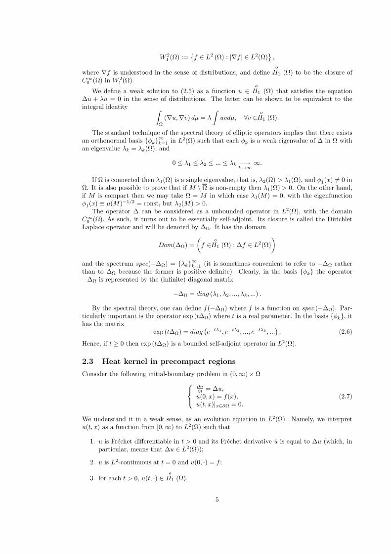
φ1

φ2

φ3

L2(Ω)

f

u(t, )

Figure 1 Function u(t, x) as a path in L2(Ω)

It is easy to verify that the evolution equation u = ∆u has solution

u = et∆Ωf. (2.8)

Let us write this down in the basis φk. The function f ∈ L2(Ω) has the following expansionin this basis

f =∞∑k=1

akφk

whereak =

∫Ω

f(y)φk(y)dµ(y) .

Then, by (2.6),

et∆Ωf(x) =∞∑k=1

ake−tλk(Ω)φk(x)

=∞∑k=1

e−tλk(Ω)φk(x)∫

Ω

f(y)φk(y)dµ(y)

=∫

Ω

∞∑k=1

e−tλk(Ω)φk(x)φk(y)

f(y)dµ(y).

The kernel in the curly brackets is called the heat kernel of Ω and will be denoted by pΩ(t, x, y).Hence, we have

pΩ(t, x, y) :=∞∑k=1

e−tλk(Ω)φk(x)φk(y) (2.9)

and the weak solution u(t, x) to (2.7) is given by

u(t, x) = et∆Ωf =∫

Ω

pΩ(t, x, y)f(y)dµ(y). (2.10)

Note that (2.10) is just another way to write down (2.8). Hence, the operator et∆Ω has theintegral kernel pΩ(t, x, y).

The eigenfunction φk(x) are C∞-smooth, by the local elliptic regularity. The sequence λkobeys Weyl’s asymptotic formula

λk(Ω) ∼ cn

(k

µ(Ω)

)2/n

, k → ∞,

6

and, hence, is growing fast enough to ensure convergence of (2.9) locally in any Cm(Ω). Hence,pΩ ∈ C∞((0,∞) × Ω × Ω). The solution u(t, x) defined by (2.10) is then C∞-smooth andsatisfies the heat equation in the classical sense. If f is continuous then it is possible to showthat u(t, x) is continuous in the classical sense in [0,∞) × Ω and u(t, x) = f(x).

Since φk ∈o

H1 (Ω), we obtain that pΩ is also ino

H1 (Ω) as a function of x (or y). If theboundary ∂Ω is smooth, then this implies that pΩ(t, x, y) extends continuously to Ω and that pΩ

vanishes on ∂Ω. In particular, the function u defined by (2.10) is also continuous on (0,∞)×∂Ωand u(t, x) = 0 for all t > 0 and x ∈ ∂Ω.

Other simple properties of pΩ are as follows:

(a) As a function of t and x, the function pΩ(t, x, y) satisfies the heat equation

∂pΩ

∂t= ∆pΩ

and the initial valuepΩ(t, ·, y) → δy as t→ 0 + .

(b) The semigroup property: for all t, s > 0 and x, y ∈ Ω,

pΩ(t+ s, x, y) =∫

Ω

pΩ(t, x, z)pΩ(s, x, y)dµ(z), (2.11)

which is another way to write down the identity e(t+s)∆Ω = et∆Ωes∆Ω .

(c) The symmetrypΩ(t, x, y) = pΩ(t, y, x). (2.12)

The latter is obvious from (2.9) but would not be so transparent if we were to define pΩ asa kernel which solves the initial-boundary problem (2.7) by (2.10).

If Ω is connected and M \ Ω is non-empty then λ1(Ω) > 0 is a single eigenvalue, φ1(x) = 0in Ω, and (2.9) implies

pΩ(t, x, y) ∼ e−tλ1(Ω)φ1(x)φ1(y), t→ ∞. (2.13)

If M is compact then we may take Ω = M in which case (2.9) yields

pM (t, x, y) =1

µ(M)+

∞∑k=2

e−tλk(M)φk(x)φk(y). (2.14)

In particular, we havepM (t, x, y) → µ(M)−1, t→ ∞. (2.15)

2.4 Maximum principle and positivity of the heat kernel

The properties of the heat kernel pΩ discussed above follows from the self-adjointness of theLaplace operator in L2(Ω). However, there is another aspect of the Laplace operator whichcannot be derived only from the spectral properties. For example, it is known that pΩ(t, x, y) > 0for all t > 0 and x, y ∈ Ω. However, the positivity of the heat kernel is not at all obvious fromthe eigenfunction expansion (2.9), because the eigenfunctions φk are signed (except for φ1).

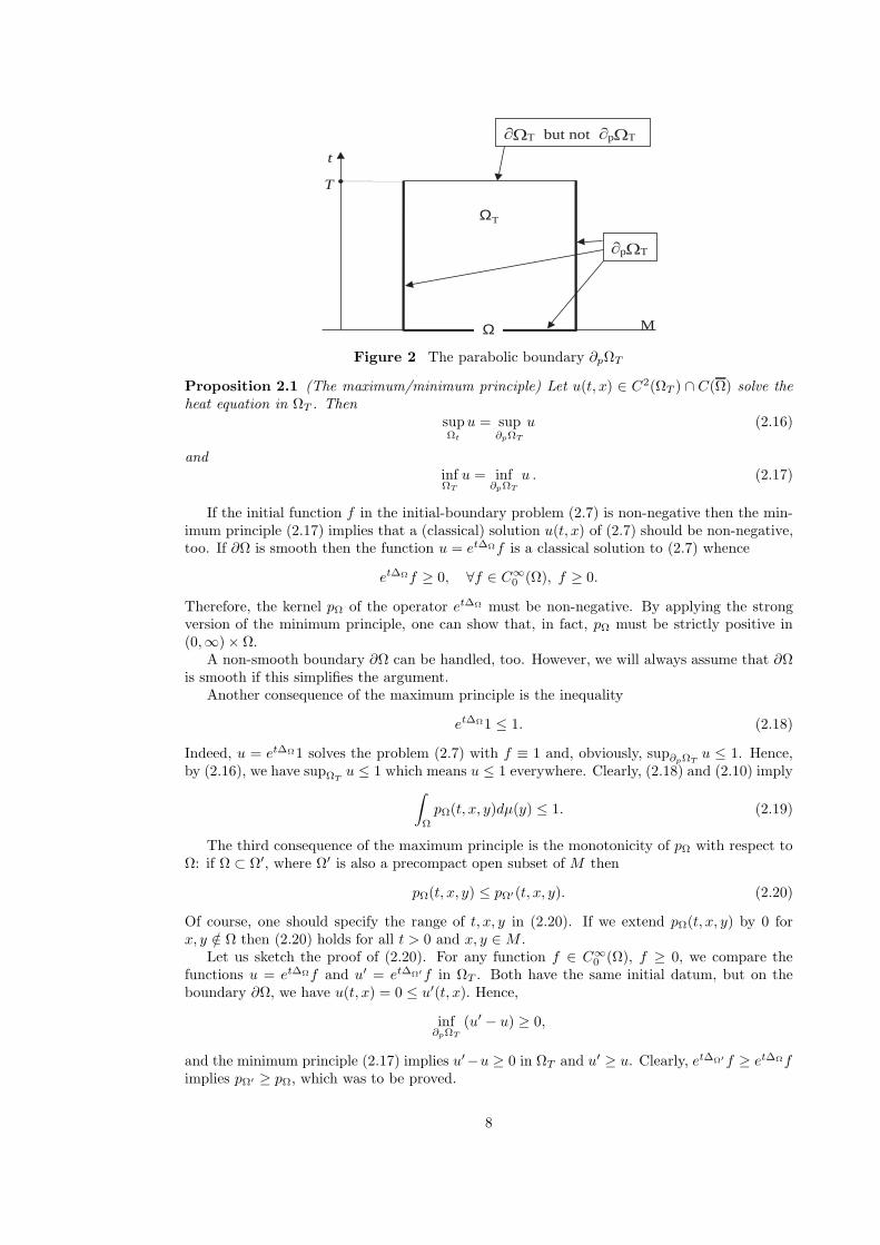
Here we consider another property of the heat equation which is called the maximum(minimum) principle and which is responsible for the positivity of the heat kernel. DenoteΩT = (0, T )× Ω, which is a cylinder in [0,∞)×M , and define its parabolic boundary ∂pΩT by

∂pΩT := ∂ΩT \ (t, x) : t = T .

In other words, ∂pΩT is the part of the boundary ∂Ω without the top of the cylinder.

7

t

T

ΩΩ M

ΩT

p T

T but not p T

Figure 2 The parabolic boundary ∂pΩT

Proposition 2.1 (The maximum/minimum principle) Let u(t, x) ∈ C2(ΩT ) ∩ C(Ω) solve theheat equation in ΩT . Then

supΩt

u = sup∂pΩT

u (2.16)

andinfΩT

u = inf∂pΩT

u . (2.17)

If the initial function f in the initial-boundary problem (2.7) is non-negative then the min-imum principle (2.17) implies that a (classical) solution u(t, x) of (2.7) should be non-negative,too. If ∂Ω is smooth then the function u = et∆Ωf is a classical solution to (2.7) whence

et∆Ωf ≥ 0, ∀f ∈ C∞0 (Ω), f ≥ 0.

Therefore, the kernel pΩ of the operator et∆Ω must be non-negative. By applying the strongversion of the minimum principle, one can show that, in fact, pΩ must be strictly positive in(0,∞) × Ω.

A non-smooth boundary ∂Ω can be handled, too. However, we will always assume that ∂Ωis smooth if this simplifies the argument.

Another consequence of the maximum principle is the inequality

et∆Ω1 ≤ 1. (2.18)

Indeed, u = et∆Ω1 solves the problem (2.7) with f ≡ 1 and, obviously, sup∂pΩTu ≤ 1. Hence,

by (2.16), we have supΩTu ≤ 1 which means u ≤ 1 everywhere. Clearly, (2.18) and (2.10) imply∫

Ω

pΩ(t, x, y)dµ(y) ≤ 1. (2.19)

The third consequence of the maximum principle is the monotonicity of pΩ with respect toΩ: if Ω ⊂ Ω′, where Ω′ is also a precompact open subset of M then

pΩ(t, x, y) ≤ pΩ′(t, x, y). (2.20)

Of course, one should specify the range of t, x, y in (2.20). If we extend pΩ(t, x, y) by 0 forx, y /∈ Ω then (2.20) holds for all t > 0 and x, y ∈M .

Let us sketch the proof of (2.20). For any function f ∈ C∞0 (Ω), f ≥ 0, we compare the

functions u = et∆Ωf and u′ = et∆Ω′f in ΩT . Both have the same initial datum, but on theboundary ∂Ω, we have u(t, x) = 0 ≤ u′(t, x). Hence,

inf∂pΩT

(u′ − u) ≥ 0,

and the minimum principle (2.17) implies u′−u ≥ 0 in ΩT and u′ ≥ u. Clearly, et∆Ω′f ≥ et∆Ωfimplies pΩ′ ≥ pΩ, which was to be proved.

8

2.5 Heat semigroup on a manifold

The monotonicity of the heat kernel pΩ with respect in Ω allows to construct the heat kernel pon the entire manifold M by taking the limit as “Ω →M”. The latter means that we consideran exhaustion sequence Ωk that is a sequence of precompact open sets Ωk ⊂ M such that∂Ωk is smooth, Ωk ⊂ Ωk+1 and

∞⋃k=1

Ωk = M .

Such sequence can be constructed on any manifold. Then we define

p(t, x, y) := limk→∞

pΩk(t, x, y). (2.21)

Since pΩk+1 ≥ pΩk, the limit exists (finite or infinite) and does not depend on the choice of

Ωk. As follows from (2.19), ∫M

p(t, x, y)dµ(y) ≤ 1,

so that p is finite almost everywhere. By the convergence properties of solutions to the parabolicequations, p(t, x, y) is finite everywhere and C∞-smooth.

Clearly, p(t, x, y) inherits all previously discussed properties of pΩ(t, x, y) except for theeigenfunction expansion (2.9). Moreover, it is possible to define the Dirichlet extension ofthe Laplace operator ∆ on M (denote it ∆M ) and to show that p(t, x, y) is the kernel of thesemigroup et∆M acting in L2(M) (see [55]). However, the spectrum of ∆M is not necessarilydiscrete as for a precompact region Ω. This is why it is not possible in general to define theheat kernel by the eigenfunction expansion (2.9).

After the heat kernel has been constructed by (2.21), we can give a shorter definition.

Definition 2.2 The heat kernel p(t, x, y) on M is the smallest positive fundamental solutionto the heat equation on (0,∞) ×M .

A “fundamental solution” means that∂p∂t = ∆xp,p(t, ·, y) −→

t→0δy.

(2.22)

If q(t, x, y) is another positive fundamental solution then the minimum principle implies q ≥ pΩ

for any precompact region Ω. By (2.21), we obtain q ≥ p and p is the smallest one.The purpose of all constructions in this section was to provide the (sketch of) proof of

the existence of the smallest positive fundamental solution and to obtain its most importantproperties. The full justification of the above constructions can be found in [55], [22].

As an example of application, let us consider a direct Riemannian product M = M ′ ×M ′′

whereM ′ andM ′′ are Riemannian manifolds. It is easy to see that ∆ = ∆′+∆′′ and µ = µ′×µ′′,where the dashes refer to the manifolds M ′ and M ′′, respectively. The heat kernel on M is alsoa direct product of the heat kernels in M ′ and M ′′, that is,

p(t, x, y) = p′(t, x′, y′)p′′(t, x′′, y′′) , (2.23)

where x = (x′, x′′) ∈M and y = (y′, y′′) ∈M . Indeed, one first proves the obvious modificationof (2.23) for a precompact region Ω = Ω′ × Ω′′ ⊂ M directly by (2.9), and then passes to thelimit as in (2.21).

In particular, the heat kernel (1.1) in Rn can be obtained from the heat kernel in R1 byiterating (2.23). If M ′ = Rm and M ′′ = K where K is a compact manifold then, by (2.23),(1.1) and (2.15), the heat kernel on M = Rm ×K has the following asymptotic

p(t, x, x) ∼ µ′′(K)−1 (4πt)−m/2 , t→ ∞. (2.24)

9

3 Integral estimates of the heat kernel

In this section, we introduce an integral version of the maximum principle and apply it toestimate some integrals of the heat kernel.

3.1 Integral maximum principle

Lemma 3.1 (Aronson [4]) Let Ω ⊂M be a precompact region. Suppose that u(t, x) ∈ C2(ΩT

)solves the heat equation in ΩT and satisfies the boundary condition u|∂Ω = 0. Let ξ(t, x) be alocally Lipschitz function on (0,∞) ×M such that

ξt +12|∇ξ|2 ≤ 0. (3.1)

Then the function

J(t) :=∫

Ω

u2(t, x)eξ(t,x)dµ(x) (3.2)

is non-increasing in t.

Why is this called a maximum principle? Indeed, assume u ≥ 0 and consider anotherfunction

S(t) = supx∈Ω

u(t, x).

By applying (2.16) in Ωs,t := (s, t) × Ω where t > s > 0, we obtain

S(s) = sup∂pΩs,t

u = supΩs,t

u ≥ S(t),

that is, S(t) is non-increasing.It is possible to prove that the following function

Sα(t) = ‖u(·, t)‖Lα(Ω)

is non-increasing for all α ∈ [1,∞]. If α = 2 then this amounts to Lemma 3.1 with ξ ≡ 0.Hence, Lemma (3.1) is a weighted version of the fact that S2(t) is non-increasing, whereas theclassical maximum principle implies that S∞(t) is non-increasing.

Non-trivial examples of function ξ satisfying (3.1) are as follows:

ξ(t, x) =d2(x)

2t

and

ξ(t, x) = ad(x) − a2

2t, a ∈ R,

provided d(x) is a Lipschitz function such that

|∇d| ≤ 1.

Proof of Lemma 3.1. Let us differentiate J(t) and show that J ′ ≤ 0. Indeed, we have, byusing ξt ≤ − 1

2 |∇ξ|2, ut = ∆u and by (2.3),

J ′(t) =∫

Ω

u2ξteξ + 2

∫Ω

uuteξ

≤ −12

∫Ω

u2 |∇ξ|2 eξ + 2∫

Ω

u∆u eξ

= −12

∫Ω

u2 |∇ξ|2 eξ − 2∫

Ω

u (∇u,∇ξ) eξ − 2∫

Ω

|∇u|2 eξ

= −12

∫Ω

(u∇ξ + 2∇u)2 eξ, (3.3)

10

which is non-positive.One can get from (3.3) a sharper estimate for the decay of J(t). Indeed, let us observe that

12

(u∇ξ + 2∇u)2 eξ = 2|∇(ueξ/2)|2.

By the variational property of λ1 (Ω),∫Ω

|∇(ueξ/2)|2dµ ≥ λ1 (Ω)∫

Ω

|ueξ/2|2 = λ1 (Ω)J(t).

Hence, (3.3) yields J ′ ≤ −2λ1 (Ω) J whence

J(t) ≤ J(t0) exp (−2λ1 (Ω) (t− t0)) , ∀t ≥ t0 > 0. (3.4)

If ξ(t, x) ≡ 0 and u(t, x) = pΩ(t, x, x0) then, by (2.12) and (2.11),

J(t) =∫

Ω

p2Ω(t, x, x0)dµ(x) = pΩ(2t, x0, x0).

Therefore, as a consequence of Lemma 3.1, pΩ(t, x0, x0) is non-increasing in t. By lettingΩ M we see that p(t, x0, x0) is non-increasing in t either.

3.2 The Davies inequality

The following theorem shows why the Gaussian exponential term is relevant to the heat kernelupper bounds on arbitrary manifolds.

Theorem 3.2 (Davies [45]) Let M be an arbitrary Riemannian manifold and let A and B betwo µ-measurable sets on M . Then∫

A

∫B

p(t, x, y)dµ(x)dµ(y) ≤√µ(A)µ(B) exp

(−d

2(A,B)4t

), (3.5)

where d(A,B) is the geodesic distance between A and B (if A and B intersect then d(A,B) = 0).

The first proof. By the approximation argument, it suffices to prove (3.5) for compact Aand B. Furthermore, if A and B are compact then it suffices to prove (3.5) for the heat kernelpΩ of any precompact open set Ω containing A and B.

ABd(A,B)

Ω

Figure 3 Sets A and B

Consider the function u(t, x) = et∆Ω1A. We can write∫B

∫A

pΩ(t, x, y)dµ(y)dµ(x) =∫B

(∫Ω

pΩ(t, x, y)1Adµ(y))dµ(x)

=∫B

u(t, x)dµ(x)

≤ µ(B)1/2(∫

B

u2(t, x)dµ(x))1/2

. (3.6)

11

Let us set, for some α > 0,

ξ(t, x) := αd(x,A) − α2

2t

and consider the functionJ(t) :=

∫Ω

u2(t, x)eξ(t,x)dµ(x) ,

which, by Lemma (3.1) is non-increasing in t > 0. If x ∈ B then

ξ(t, x) ≥ αd(B,A) − α2

2t,

whence

J(t) ≥∫B

u2(t, x)eξ(t,x)dµ(x)

≥ exp(αd(A,B) − α2

2t

)∫B

u2(t, x)dµ(x). (3.7)

On the other hand, if x ∈ A then ξ(0, x) = 0. By the continuity of J(t) at t = 0+, we have

J(t) ≤ J(0) =∫

Ω

eξ(0,x)1Adµ(x) = µ(A). (3.8)

Combining (3.6), (3.7) and (3.8), we obtain∫A

∫B

pΩ(t, x, y)dµ(x)dµ(y) ≤√µ(A)µ(B) exp

(−α

2d(A,B) +

α2

4t

).

Setting here α = d(A,B)/t we finish the proof.

Remark 3.3 Using (3.4) instead of the monotonicity of J gives the better inequality∫A

∫B

p(t, x, y)dµ(x)dµ(y) ≤√µ(A)µ(B) exp

(−λ1(M)t− d2(A,B)

4t

), (3.9)

whereλ1 (M) := inf

Ω⊂⊂Mλ1 (Ω) . (3.10)

It is possible to show that λ1(M) is the bottom of the spectrum of the operator −∆M inL2(M,µ). Sometimes λ1(M) is called the spectral radius of the manifold M .

The second proof. Assume again that A and B are two compact subsets of a precompactregion Ω. Fix some Lipschitz function ψ(x) on Ω and consider the integral

J(t) :=∫

Ω

u2(t, x)eψ(x)dµ(x),

where u(t, x) solves the heat equation in R+ ×Ω and vanishes on ∂Ω. Easy computation showsthat

J ′(t) = 2∫

Ω

u∆u eψ = −2∫

Ω

|∇u|2 eψ − 2∫

Ω

ueψ (∇u,∇ψ) .

Applying the inequality

−2u (∇u,∇ψ) ≤ 2 |∇u|2 +12u2 |∇ψ|2 ,

we obtainJ ′(t) ≤ 1

2

∫Ω

u2eψ |∇ψ|2 dµ. (3.11)

12

Let us set ψ(x) = αd(x,A), for some α > 0. Then |∇ψ| ≤ α and (3.11) implies J ′ ≤ 12α

2Jwhence

J(t) ≤ J(0) exp(12α2t). (3.12)

Let us apply the above to the function u = et∆Ω1A. Since

J(0) =∫

Ω

1A exp (αd(x,A)) dµ(x) = µ(A) ,

(3.12) implies ∫Ω

u2(t, x) exp (αd(x,A)) dµ(x) ≤ µ(A) exp(12α2t)

and ∫B

u2(t, x)dµ(x) ≤ µ(A) exp(−αd(A,B) +

12α2t

).

Choosing α = d(A,B)/t and applying (3.6), we finish the proof.The third proof. This proof is less elementary than the previous two, but it yields the

better estimate:∫A

∫B

p(t, x, y)dµ(x)dµ(y) ≤√µ(A)µ(B)

∫ ∞

δ

1√πt

exp(−s

2

4t

)ds, (3.13)

where δ = d(A,B). Indeed, it is possible to prove that∫ ∞

δ

1√πt

exp(−s

2

4t

)ds ≤ min(1,

2√π

√t

δ) exp

(−δ

2

4t

). (3.14)

Therefore, (3.13) is better than (3.5) when δ >>√t.

The inequality (3.13) is a particular case of a more general inequality of Cheeger, GromovTaylor [27, Proposition 1.1], which says the following. Let φ ∈ L1(R+) and Φ be its cos-Fouriertransform, that is,

Φ(λ) =∫ ∞

0

φ(s) cos(sλ)ds. (3.15)

The function Φ is bounded and continuous so that we can consider the bounded operatorΦ(

√−∆M ) in L2(M,µ) in the sense of the spectral theory. Then, for any function f ∈ L2(M,µ)and any δ > 0, we have∥∥∥Φ(

√−∆M ) f

∥∥∥L2(M\suppδf)

≤ ‖f‖∫ ∞

δ

|φ(s)| ds (3.16)

where suppδf means the δ-neighborhood of supp f and ‖·‖ = ‖·‖L2(M).Given (3.16), let us take another function g ∈ L2(M,µ) and suppose that the distance

between the supports of f and g is at least δ. Then (3.16) yields∫M

gΦ(√

−∆M

)f dµ ≤ ‖f‖ ‖g‖

∫ ∞

δ

|φ(s)| ds (3.17)

(see also [32, Proposition 3.1]). Fix some t > 0 and take

φ(s) =1√πt

exp(−s

2

4t

).

Then Φ(λ) = exp(−tλ2

)and Φ(

√−∆M ) = exp (t∆M ) which is the heat semigroup. Hence,(3.17) implies

∫M

∫M

g(x)p(t, x, y)f(y)dµ(y)dµ(x) ≤ ‖f‖ ‖g‖∞∫δ

1√πt

exp(−s

2

4t

)ds,

13

and (3.13) follows by taking f = 1A and g = 1B.The proof of (3.16) is based on the fact that the function

u(t, ·) = cos(t√

−∆M )f

solves the Cauchy problem for the wave equationutt = ∆uu|t=0 = f and ut|t=0 = 0.

The wave equation possesses the finite propagation speed equal to 1, which means that thesupport of the solution at time t lies in the t-neighborhood of the support of the initial data.Hence,

suppu(t, ·) ⊂ supptf . (3.18)

Denote w = Φ(√−∆M ) f . Then, by (3.15),

w(x) =∫ ∞

0

φ(s) cos(s√−∆M )f(x)ds =

∫ ∞

0

φ(s)u(s, x)ds.

If x /∈ supptf then, by (3.18), u(s, x) = 0 for all s ≤ t. Hence, for those x, we have

w(x) =∫ ∞

t

φ(s)u(s, x)ds =∫ ∞

t

φ(s) cos(s√−∆M )f(x)ds

and, using |cos| ≤ 1,

‖w‖L2(M\supptv)≤

∫ ∞

t

φ(s)∥∥∥cos(s

√−∆M )

∥∥∥L2→L2

‖f‖ds

= ‖f‖∫ ∞

t

φ(s)ds,

which was to be proved.Lemma 3.1 and Theorem 3.2 can be used for obtaining heat kernel upper and lower bounds,

estimating the eigenvalues of the Laplace operator, obtaining conditions for stochastic com-pleteness etc. Some of the applications are show in the next sections.

3.3 Stochastic completeness

A Riemannian manifold M is called stochastically complete if, for all x ∈M and t > 0,∫M

p(t, x, y)dµ(y) = 1. (3.19)

In term of the Brownian motion Xt, (3.19) means that the total probability of Xt to be foundon M is equal to 1. The opposite can happen, for example, if M is an open bounded region onRn and Xt is the Brownian motion on M with the killing boundary conditions on ∂M . Indeed,the process Xt riches the boundary in finite time with positive probability and then Xt stopsexisting as a point in M , which makes the integral in (3.19) smaller than 1. However, Azencott[5] showed that even a geodesically complete manifold may be stochastically incomplete. Onsuch a manifold, the Brownian particle moves away extremely fast so that it covers an infinitedistance in a finite time. This happens for a geometric reason - the manifold like that has a lotof space in a neighborhood of infinity which “draws” there a Brownian particle.

The following theorem provides a test for stochastic completeness in terms of the volumegrowth.

Theorem 3.4 ([65]) Let M be a geodesically complete manifold. Assume that, for some pointx ∈M , ∫ ∞ rdr

logV (x,R)= ∞, (3.20)

where V (x, r) = µ(B(x, r)). Then M is stochastically complete.

14

For example, (3.20) holds if V (x,R) ≤ C exp(CR2

). In particular, a geodesically complete

manifold with bounded below Ricci curvature is stochastically complete. This was first provedby Yau [140].

The proof of Theorem 3.4 can be found in [65] and [74]. It uses the same approach asin the proof of Lemma 3.1 but in a more sophisticated way. A reader interested in furtherconsideration of stochastic completeness and related questions is referred to the survey [74].

4 Eigenvalues estimates

In this section we show an application of Theorem 3.2 for eigenvalue estimates. Let M be acompact connected Riemannian manifold. Denote by

0 = λ1 < λ2 ≤ λ3 ≤ ... ≤ λk ≤ ...

the eigenvalues of −∆M and by φk(x) their corresponding eigenfunctions forming an orthonor-mal basis in L2(M).

Theorem 4.1 (Chung – Grigor’yan – Yau [31]) Let M be a compact Riemannian manifold.Let A1, A2,...,Ak be k disjoint closed set on M . Denote

δ := mini=j

d(Ai, Aj).

Then

λk ≤ 4δ2

maxi=j

(log

2µ(M)√µ(Ai)µ(Aj)

)2

. (4.1)

In particular, if we have two sets A1 = A and A2 = B then (4.1) becomes

λ2(M) ≤ 4δ2

(log

2µ(M)√µ(A)µ(B)

)2

, (4.2)

where δ = d(A,B).

A1A2

Μ

A3

Ak

δ

Figure 4 Sets Ai on a compact manifold M

Proof. We first prove (4.2). By the eigenfunction expansion (2.9), we can write, for any t > 0,∫A

∫B

p(t, x, y)dµ(x)dµ(y) =∞∑i=1

e−tλi

∫A

φi(x)dµ(x)∫B

φi(y)dµ(y).

Denoteai :=

∫A

φi(x)dµ(x) = (1A, φi)L2(M) , bi := (1B, φi)L2(M)

15

and observe that ai and bi are the Fourier coefficients of the functions 1A and 1B in the basisφi, whence

∞∑i=1

a2i = ‖1A‖2

L2(M) = µ(A) and∞∑i=1

b2i = µ(B).

Since φ1 ≡ 1/√µ(M) (cf. (2.14)), we obtain

a1 = (1A,1õ(M)

)L2(M) =µ(A)√µ(M)

and b1 =µ(B)√µ(M)

.

Thus, we have

∫A

∫B

p(t, x, y)dµ(X)dµ(y) = a1b1 +∞∑i=2

e−tλiaibi

≥ a1b1 − e−tλ2

( ∞∑i=2

a2i

)1/2 ( ∞∑i=2

b2i

)1/2

≥ µ(A)µ(B)µ(M)

− e−tλ2√µ(A)µ(B).

Comparing with the Davies inequality (3.5), we obtain

√µ(A)µ(B)e−

δ24t ≥ µ(A)µ(B)

µ(M)− e−tλ2

√µ(A)µ(B)

and

e−tλ2 ≥√µ(A)µ(B)µ(M)

− e−δ24t

Choosing t so that

e−δ24t =

12

√µ(A)µ(B)µ(M)

,

we conclude

λ2 ≤ 1t

log2µ(M)√µ(A)µ(B)

=4δ2

(log

2µ(M)√µ(A)µ(B)

)2

,

which is (4.2).Let us now turn to the case k > 2. Consider the following integrals

Jlm :=∫Al

∫Am

p(t, x, y)dµ(x)dµ(y)

and denotea(l)i := (1Al

, φi).

Then exactly as above, we have

Jlm =∞∑i=1

a(l)i a

(m)j

=µ(Al)µ(Am)

µ(M)+k−1∑i=2

e−λita(l)i a

(m)i +

∞∑i=k

e−λita(l)i a

(m)i

≥ µ(Al)µ(Am)µ(M)

+k−1∑i=2

e−λita(l)i a

(m)i − e−λkt

√µ(Al)µ(Am). (4.3)

16

On the other hand, by Theorem 3.2,

Jlm ≤√µ(Al)µ(Am)e−

δ24t . (4.4)

Therefore, we can further argue as in the case k = 2 provided the middle term in (4.3) can bediscarded, that is,

k−1∑i=2

e−λita(l)i a

(m)i ≥ 0. (4.5)

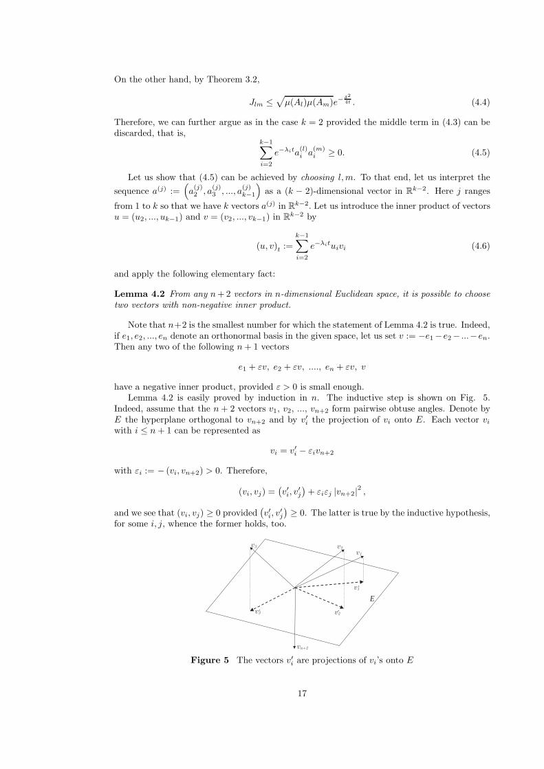
Let us show that (4.5) can be achieved by choosing l,m. To that end, let us interpret thesequence a(j) :=

(a(j)2 , a

(j)3 , ..., a

(j)k−1

)as a (k − 2)-dimensional vector in Rk−2. Here j ranges

from 1 to k so that we have k vectors a(j) in Rk−2. Let us introduce the inner product of vectorsu = (u2, ..., uk−1) and v = (v2, ..., vk−1) in Rk−2 by

(u, v)t :=k−1∑i=2

e−λituivi (4.6)

and apply the following elementary fact:

Lemma 4.2 From any n+ 2 vectors in n-dimensional Euclidean space, it is possible to choosetwo vectors with non-negative inner product.

Note that n+2 is the smallest number for which the statement of Lemma 4.2 is true. Indeed,if e1, e2, ..., en denote an orthonormal basis in the given space, let us set v := −e1−e2− ...−en.Then any two of the following n+ 1 vectors

e1 + εv, e2 + εv, ...., en + εv, v

have a negative inner product, provided ε > 0 is small enough.Lemma 4.2 is easily proved by induction in n. The inductive step is shown on Fig. 5.

Indeed, assume that the n+ 2 vectors v1, v2, ..., vn+2 form pairwise obtuse angles. Denote byE the hyperplane orthogonal to vn+2 and by v′i the projection of vi onto E. Each vector viwith i ≤ n+ 1 can be represented as

vi = v′i − εivn+2

with εi := − (vi, vn+2) > 0. Therefore,

(vi, vj) =(v′i, v

′j

)+ εiεj |vn+2|2 ,

and we see that (vi, vj) ≥ 0 provided(v′i, v

′j

) ≥ 0. The latter is true by the inductive hypothesis,for some i, j, whence the former holds, too.

E

Figure 5 The vectors v′i are projections of vi’s onto E

17

Let us finish the proof of Theorem 4.1. Fix some t > 0. By Lemma 4.2, we can find l,m sothat

(a(l), a(m)

)t≥ 0 and (4.5) holds. Then (4.3) and (4.4) yield

e−tλk ≥√µ(Al)µ(Am)µ(M)

− e−δ24t ,

and we are left to choose t. However, t should not depend on l,m because we use t to definethe inner product (4.6) before choosing l,m. So, we first write

e−tλk ≥ mini,j

√µ(Ai)µ(Aj)µ(M)

− e−δ24t

and then define t by

e−δ24t =

12

mini,j

√µ(Ai)µ(Aj)µ(M)

,

whence (4.1) follows.Somewhat sharper estimates of the eigenvalues can be obtained by using (3.13) instead of

(3.5) - see [32].

5 Pointwise estimates of the heat kernel

We discuss here two methods of obtaining the Gaussian upper bounds of the heat kernelp(t, x, y), that is, the estimates containing the factor exp

(− d2

Ct

)where d = d(x, y). The first

approach is based on properties of weighted integrals of the heat kernel in the spirit of Lemma3.1. The second method is based on Theorem 3.2 and on certain mean-value inequality.

5.1 Gaussian upper bounds for the heat kernel

Let M be so far an arbitrary Riemannian manifold. We start we an observation that

p(t, x, x) =∫M

p2(t/2, x, z)dµ(z) (5.1)

which follows from the semigroup identity (2.11) and the symmetry (2.12) of the heat kernel.Using the semigroup identity again and the Cauchy–Schwarz inequality, we obtain

p(t, x, y) =∫M

p(t/2, x, z)p(t/2, y, z)dµ(z)

≤(∫

M

p2(t/2, x, z)dµ(z)) 1

2(∫

M

p2(t/2, y, z)dµ(y)) 1

2

,

whence, by (5.1),p(t, x, y) ≤

√p(t, x, x)p(t, y, y). (5.2)

For example, if we knew an on-diagonal estimate like

p(t, x, x) ≤ f(t), ∀x ∈M,

it would imply the off-diagonal estimate

p(t, x, y) ≤ f(t), ∀x, y ∈M.

However, the latter does not take into account the distance between x and y. To fix that, wewill modify the above argument to introduce the Gaussian factor.

18

Let us consider the following weighted integral of the heat kernel:

ED(t, x) :=∫M

p2(t, x, z) exp(d2(x, z)Dt

)dµ(z), (5.3)

where D > 0 will be specified later. In the limit case D = ∞, we obtain by (5.1)

E∞(t, x) = p(2t, x, x), (5.4)

and (5.2) can be rewritten as

p(t, x, y) ≤√E∞(t/2, x)E∞(t/2, y).

It turns out that a similar estimate holds for a finite D.

Lemma 5.1 ([69, Proposition 5.1])We have, for any D > 0 and all x, y ∈M , t > 0,

p(t, x, y) ≤√ED(t/2, x)ED(t/2, y) exp

(−d

2(x, y)2Dt

). (5.5)

Proof. For any points x, y, z ∈ M, let us denote α = d(y, z), β = d(x, z) and γ = d(x, y). Bythe triangle inequality, α2 + β2 ≥ 1

2γ2.

β

α

γ

x

z

y

Figure 6 Distances α, β, γ

We have then

p(t, x, y) =∫M

p(t/2, x, z)p(t/2, y, z)dµ(z)

≤∫M

p(t/2, x, z)eβ2

Dt p(t/2, y, z)eα2Dt e−

γ2

2Dt dµ(z)

≤(∫

M

p2(t/2, x, z)e2β2Dt dµ(z)

) 12(∫

M

p2(t/2, y, z)e2α2Dt dµ(y)

) 12

e−γ22Dt

=√ED(t/2, x)ED(t/2, y) exp

(−d

2(x, y)2Dt

),

which was to be proved.It is not a priori clear that ED(t, x) is finite. Indeed, it is easy to see that in Rn, ED = ∞

for all D ≤ 2. Nevertheless, the following is true.

Theorem 5.2 ([66], [69]) For any manifold M , ED(t, x) is finite for all D > 2, t > 0, x ∈M .Moreover, ED(t, x) is non-increasing in t.

The most non-trivial part of this theorem is the finiteness of ED. The non-increasing of EDis an immediate consequence of Lemma 3.1.

Furthermore, the functionED(t, x) exp (2λ1(M)t)

19

is also non-increasing in t, which follows from (3.4) (recall that the spectral radius λ1(M) isdefined by (3.10)). Inequality (5.5) implies, for all t0 > 0 and t > 0,

p(t, x, y) ≤√ED(τ/2, x)ED(τ/2, y)eλ1(M)t0 exp

(−λ1(M)t− d2(x, y)

2Dt

), (5.6)

where τ = min(t, t0). Indeed, if t ≥ t0 then (5.6) follows from (5.5) and

ED (t/2, x) exp (λ1(M)t) ≤ ED(t0/2) exp (λ1(M)t0) . (5.7)

If t < t0 then (5.6) follows from (5.5) directly.If λ1(M) > 0 then (5.6) provides already a good upper bound of the heat kernel which can

be rewritten as follows, for t > t0,

p(t, x, y) ≤ Φ(x, y) exp(−λ1(M)t− d2(x, y)

2Dt

), (5.8)

whereΦ(x, y) :=

√ED(t0/2, x)ED(t0/2, y)eλ1(M)t0 .

However, if λ1(M) = 0 then (5.6) is of no use and, by Lemma 5.1, the question of obtainingthe long time behaviour of p(t, x, y) amounts to the same question for ED(t, x). The latter isreduced by the following theorem to the on-diagonal rate of decay of p(t, x, x) in t.

Theorem 5.3 (Ushakov [129], Grigor’yan [72]) Assume that, for some x ∈ M and for allt > 0,

p(t, x, x) ≤ C

f(t), (5.9)

where f(t) is an increasing positive function on (0,+∞) satisfying certain regularity condition( see below). Then, for all D > 2 and t > 0,

ED(t, x) ≤ C′

f(εt), (5.10)

for some ε > 0 and C′.

Remark 5.4 If (5.9) holds for t ≤ t0 then (5.10) also holds for t ≤ t0. Indeed, extend thefunction f(t) by the constant f(t0) for t > t0. Then (5.9) is true for all t because p(t, x, x) isnon-increasing in t as was remarked at the end of Section 3.1. Hence, by Theorem 5.3, (5.10)is true, too.

The regularity condition is the following: there are numbers A ≥ 1 and a > 1 such that

f(as)f(s)

≤ Af(at)f(t)

, for all 0 < s < t. (5.11)

The constants ε and C′ in the statement of Theorem 5.3 depend on A and a. There are twosimple situations when (5.11) holds:

1. f(t) satisfies the doubling condition, that is, for some A > 1,

f(2t) ≤ Af(t), ∀t > 0. (5.12)

Then (5.11) holds with a = 2 because

f(2s)f(s)

≤ A ≤ Af(2t)f(t)

.

20

2. f(t) has at least polynomial growth in the sense that, for some a > 1, the functionf(at)/f(t) is increasing in t. Then (5.11) holds for A = 1.

If f is differentiable then (5.11) is implied by either of the following properties of the functionl(ξ) := log f(eξ) defined in (−∞,+∞):

1. l′ is uniformly bounded (for example, this is the case when f(t) = tN or f(t) = logN (1+ t)where N > 0);

2. l′ is monotone increasing (for example, f(t) = exp(tN )).

On the other hand, (5.11) fails if l′ = exp (−ξ) (it is unbounded as ξ → −∞) whichcorresponds to f(t) = exp

(−t−1). Also, (5.11) may fail if l′ is oscillating.

By putting together Theorem 5.3 and Lemma 5.1, we obtain

Corollary 5.5 Assume that, for some points x, y ∈M and for all t > 0,

p(t, x, x) ≤ C

f(t)and p(t, y, y) ≤ C

g(t), (5.13)

where f and g are increasing positive function on (0,+∞) satisfying the regularity condition(5.11) as above. Then, for all t > 0, D > 2 and for some ε > 0

p(t, x, y) ≤ C′√f(εt)g(εt)

exp(−d

2(x, y)2Dt

). (5.14)

Remark 5.6 By using (5.6) instead of (5.5) we obtain, for all t0 > 0,

p(t, x, y) ≤ C′eλ1(M)t0√f(ετ )g(ετ )

exp(−λ1(M)t− d2(x, y)

2Dt

), (5.15)

where τ = min(t, t0). Note that (5.13) may be assumed only for t ≤ t0. One can always extendf(t) and g(t) for t > t0 by the constants f(t0) and g(t0), respectively, and (5.13) will continueto be true by the non-increasing of p(t, x, x) in t.

Hence, the question of obtaining the Gaussian upper bounds of the heat kernel is reducedto obtaining the on-diagonal estimates (5.13), which will be considered in Section 6.

For the proof of Theorem 5.3, the reader is referred to [72]. The proof uses the integralmaximum principle of Lemma 3.1. Note that if f and g satisfy the doubling property (5.12)then ε in (5.14) and (5.15) can be absorbed into the constant C′.

The finiteness of ED(t, x) in Theorem 5.2 can be deduced from Theorem 5.3. All that oneneeds is the initial upper bound p(t, x, x) ≤ Cxt

−n/2 , for small t, which can be obtained byTheorem 5.8 from the next Section. See [66] or [69] for details.

Historically, the first method of obtaining the Gaussian upper bounds for the heat kernel ofa uniformly elliptic operators in Rn with variable coefficients was introduced by Aronson [4].He used the integral maximum principle but in a different way. The estimates of Aronson usethe Euclidean distance rather than the Riemannian distance associated with the coefficients.Varadhan [130], [131] first realized that the Riemannian distance should be used instead. Hisresult implies that, on any manifold,

limt→0+

t log p(t, x, y) = −14d2(x, y).

The first uniform Gaussian estimates for the heat kernel on manifolds was obtained by Cheng,Li and Yau [29], for manifolds of bounded geometry (see Section 7 below). They were laterimproved by Cheeger, Gromov and Taylor [27] by using (3.16). The sharp heat kernel estimatesfor the manifolds of non-negative Ricci curvature was obtained by Li and Yau [98]. Furtherprogress in Gaussian upper bounds (under non-curvature assumptions) is due to Davies [41],[42], [43]. See also [135]. The approach to the Gaussian bounds we have adopted here is due tothe author [69], [72].

21

5.2 Mean-value property

Here we present an alternative method of obtaining Gaussian upper bounds like (5.14), whichavoids using ED(t, x) and, instead, is based on Theorem 3.2 and on the mean-value property.This method was introduced by Davies [45]. The treatment of this section is close to that in[97] and [37].

Fix some distinct points x, y ∈M and consider the balls B(x, r), B(y, r). By Theorem 3.2,we have ∫

B(x,r)

∫B(y,r)

p(t, ξ, η)dµ(η)dµ(ξ) ≤√V (x, r)V (y, r) exp

(− (d− 2r)2+

4t

), (5.16)

where V (x, r) := µ(B(x, r)) and d = d(x, y). If we knew that the value of the heat kernel at(t, x, y) can be estimated via the integral in (5.16) then we could obtain from (5.16) an upperbound for p(t, x, y). This can be done by using the following mean-value property.

Definition 5.7 We say that the manifold M admits the mean-value property (MV) if, for allt > τ > 0, ξ ∈ M and for any positive solution u(s, η) of the heat equation in the cylinder(t− τ, t] ×B(ξ,

√τ), we have

u(t, ξ) ≤ C

τV (ξ,√τ )

t∫t−τ

∫B(ξ,

√τ)

u(s, η)dµ(η)ds. (5.17)

M

s

B( , )_

(t, )

(t- , )

us= u

t

t-

Figure 7 Cylinder (t− τ, t) ×B(ξ,√τ)

The geometric assumptions which imply (MV), will be discussed in Section 6.4. Here we onlymention that (5.17) holds, for example, if M is a geodesically complete manifold of nonnegativeRicci curvature.

Theorem 5.8 (Li – Wang [97], Coulhon – Grigor’yan [37]) Assume that the mean-value prop-erty (MV) holds on the manifold M . Then, for all x ∈M and t > 0,

p(t, x, x) ≤ C

V (x,√t). (5.18)

Moreover, for all x, y ∈M , t > 0, D > 2,

p(t, x, y) ≤ C′√V (x,

√t/2)V (y,

√t/2)

exp(−d

2(x, y)2Dt

). (5.19)

22

Hence, (5.19) holds on complete manifolds of non-negative Ricci curvature. For those man-ifolds, this estimate was first proved by different method by Li and Yau [98]. Moreover, theyproved also a matching lower bound for the heat kernel which shows that (5.19) is sharp up tothe values of the constants (see Sections 5.3 and 7.8 for the lower bounds of the heat kernel).In Rn, we have V (x,

√t) tn/2 so that (5.18) and (5.19) give the correct rate for the long time

decay of the heat kernel.Proof of Theorem 5.8. Let us start with the consequence of (2.19)∫

M

p(s, x, z)dµ(z) ≤ 1 (5.20)

and integrate it in time s: ∫ t

0

∫M

p(s, x, z)dµ(z) ≤ t.

Applying (5.17) for u = p(·, x, ·), we obtain

p(t, x, x) ≤ C

tV (x,√t)

∫ t

0

∫B(x,

√t)

p(s, x, z)dµ(z) ≤ C

V (x,√t),

which is exactly (5.18).To show (5.19), we argue similarly but use (5.16) instead of (5.20). We start with (5.17)

applied to the function u = p(·, ·, y),

p(t, x, y) ≤ C

τV (x,√τ )

t∫t−τ

∫B(x,

√τ)

p(s, ξ, y)dµ(ξ)ds, (5.21)

for some τ ∈ (0, t). On the other hand, also by (5.17) applied to the function u = p(·, ξ, ·),

p(s, ξ, y) ≤ C

τV (y,√τ )

s∫s−τ

∫B(y,

√τ)

p(θ, ξ, η)dµ(η)dθ. (5.22)

Combining (5.21) and (5.22), we see that p(t, x, y) is bounded above by

C2

τ2V (x,√τ )V (y,

√τ )

t∫t−τ

s∫s−τ

∫B(x,

√τ)

∫B(y,

√τ)

p(θ, ξ, η)dµ(η)dµ(ξ)dθds

≤ C2

τV (x,√τ)V (y,

√τ)

t∫t−2τ

∫B(x,

√τ)

∫B(y,

√τ)

p(θ, ξ, η)dµ(η)dµ(ξ)dθ ,

where we have assumed τ ≤ t/2. Using (5.16), we obtain

p(t, x, y) ≤ C2

τ√V (x,

√τ )V (y,

√τ )

t∫t−2τ

exp

(− (d− 2

√τ )2+

4θ

)dθ

≤ 2C2√V (x,

√τ)V (y,

√τ)

exp

(− (d− 2

√τ )2+

4t

). (5.23)

Choose τ = t/2 (which is the maximal τ we can take). If d ≥ C√t where C is large enough

then(d− 2

√τ)2+

4t≥ (

1 − o(C−1)) d2

4t,

23

and (5.23) implies (5.19). If d ≤ C√t then the Gaussian term in (5.19) is of the order 1, and

(5.19) follows again from (5.23) by discarding the Gaussian term in (5.23).Theorem 5.8 admits a localized version. We say that the manifold M admits a restricted

mean-value property (MVxyτ 0), for some x, y ∈M and τ0 ∈ R+, if the inequality (5.17) holdsfor all τ ∈ (0, τ0] and for ξ = x and ξ = y. If M admits (MVxyτ0) then a slight modificationof the above proof yields the estimate

p(t, x, y) ≤ C′√V (x,

√τ )V (y,

√τ )

exp(−λ1(M)t− d2(x, y)

2Dt

)(5.24)

where τ = min(t/2, τ0). The term λ1(M)t appears if one applies (3.9) instead of (3.5) and usesthe boundedness of τ .

Observe that the property (MVxyτ 0) holds on any manifold. Namely, for any given x, y ∈M , there exists τ0 such that (MVxyτ0) is true (which provides another proof of (5.8)). However,the constant C in the mean-value inequality (5.17) depends on the certain geometric propertiesof the balls B(x,

√τ0) and B(y,

√τ0).

If the volume function V (x, ·) satisfies the doubling condition (5.12) then (5.19) follows alsofrom (5.18), by Theorem 5.3. In this case,

√t/2 in (5.19) can be replaced by

√t. It is not

known whether there exists a manifold with (MV ) for which V (x, ·) is not doubling. Assumingthe volume doubling property, one can improve the estimate (5.19) of Theorem 5.8 as follows.

Theorem 5.9 Assume that the mean-value property (MV) holds on the manifold M and, forall r′ ≥ r and x ∈M ,

V (x, r′)V (x, r)

≤ C

(r′

r

)N, (5.25)

with some N > 0. Then, for all x, y ∈M and t > 0,

p(t, x, y) ≤ C′√V (x,

√t)V (y,

√t)

(1 +

d√t

)N−1

exp(−d

2

4t

)(5.26)

where d = d(x, y).

Remark 5.10 Although (5.25) looks stronger than the doubling property for V (x, ·), thesetwo properties are, in fact, equivalent. However, we have preferred (5.25) because the exponentN enters the estimate (5.26) in the sharp way. Indeed, as was shown by Molchanov [105], if Mis the sphere Sn and x and y are conjugate points on Sn then

p(t, x, y) ∼ c

tn/2

(d√t

)n−1

exp(−d

2

4t

), t→ 0.

Hence, the exponent N − 1 in the polynomial correction term in (5.26) is sharp. See [51] forfurther results containing the polynomial correction term.

Proof. If d2 < 4t then (5.26) follows from (5.19). Assume now d2 ≥ 4t and follow the argumentof the previous proof. However, let us use (3.13) and (3.14) instead of (3.5). Then, instead of(5.23), we obtain

p(t, x, y) ≤ 4C2√V (x,

√τ)V (y,

√τ)

√t

(d− 2√τ )+

exp

(− (d− 2

√τ)2+

4t

), (5.27)

for any τ ≤ t/2. Let us choose τ = t2

d2 which smaller than t/2, by d2 > 2t. Then we have

(d− 2√τ )2

4t≥ d2

4t− d

√τ

t=d2

4t− 1.

24

Also, d− 2√τ = d− 2 td ≥ 1

2d, whence√t

d− 2√τ≤ 2

√t

d.

Finally, by (5.25),

V(x,

√τ)

= V (x,√t

√t

d) ≥ C−1V (x,

√t)(√

t

d

)N.

After substituting all these inequalities into (5.27), we obtain (5.26).For other application of the mean-value property see [95], [94], [96], [97].

5.3 On-diagonal lower bounds and the volume growth

Here we show how to apply Theorem 5.2 to obtain on-diagonal lower bounds of the heat kernel.

Theorem 5.11 (Coulhon – Grigor’yan [36]) Let M be a geodesically complete Riemannianmanifold. Assume that, for some point x ∈M and all r > r0,

V (x, r) ≤ CrN , (5.28)

with some positive constants C and N . Then, for all t > t0,

p(t, x, x) ≥ 1/4V (x,K

√t log t)

, (5.29)

where K > 0 depend on x, r0, C,N and t0 := max(r20 , e).

Proof. Take some ρ > 0 and denote Ω = B(x, ρ). By the semigroup identity, we have

p(2t, x, x) =∫M

p2(t, x, y)dµ(y)

≥∫

Ω

p2(t, x, y)dµ(y)

≥ 1µ(Ω)

(∫Ω

p(t, x, y)dµ(y))2

=1

µ(Ω)

(1 −

∫M\Ω

p(t, x, y)dµ(y)

)2

. (5.30)

In the last line, we have used the stochastic completeness of M , that is,∫M

p(t, x, y)dµ(y) = 1.

By Theorem 3.4, this follows from the geodesic completeness of M and from the volume growthhypothesis (5.28).

Next we will choose ρ = ρ(t) so that∫M\B(x,ρ)

p(t, x, y)dµ(y) ≤ 12. (5.31)

Assume for the moment that (5.31) holds. Then (5.30) yields

p(2t, x, x) ≥ 1/4V (x, ρ(t))

.

25

To match (5.29), we need to estimate ρ(t) as follows

ρ(t) ≤ const√t log t. (5.32)

Let us prove (5.31) with ρ(t) satisfying (5.32). We apply again the Cauchy–Schwarz in-equality as follows, denoting d = d(x, y) and taking some D > 2,

∫M\B(x,ρ)

p(t, x, y)dµ(y)

2

≤∫M

p2(t, x, y) exp(d2

Dt

) ∫M\B(x,ρ)

exp(− d2

Dt

)

= ED(t, x)∫

M\B(x,ρ)

exp(− d2

Dt

)dµ(y), (5.33)

where ED(t, x) is defined by (5.3). By Theorem 5.2, we have, for all t > t0,

ED(t, x) ≤ ED(t0, x) <∞. (5.34)

Since x is fixed, we can consider ED(t0, x) as a constant. Let us now estimate the integral in(5.33) assuming that ρ = ρ(t) > r0. By splitting the integral over the complement of B(x, ρ)into the sum of the integrals over the annuli B(x, 2k+1ρ) \ B(x, 2kρ), k = 0, 1, 2, ..., and usingthe hypothesis (5.28), we obtain

∫M\B(x,ρ)

exp(−d(x, y)

2

Dt

)dµ(y) ≤

∞∑k=0

exp(−4kρ2

Dt

)V (x, 2k+1ρ) (5.35)

≤ C2NρN∞∑k=0

2Nk exp(−4kρ2

Dt

). (5.36)

y

x

2k 2k+1

Figure 8 Annulus B(x, 2k+1ρ) \B(x, 2kρ)

Assuming ρ2/t ≥ 1, the sum in the line above is majorized by a geometric series whence∫M\B(x,ρ)

exp(−d(x, y)

2

Dt

)dµ(y) ≤ C′ρN exp

(− ρ2

Dt

). (5.37)

By setting ρ(t) = K√t log t with K large enough, we make the integral above arbitrarily small,

whence (5.31) follows by (5.33) and (5.34). To finish the proof, we have to make sure thatρ(t) > r0. Indeed, this follows from t > t0 = max(r20 , e) and K > 1.

One may wonder what is geometric background of the quantity ED(t0, x) which we haveinterpreted as a constant. In fact, an upper bound of it can be proved in terms of an intrinsicgeometric property of the ball B(x, ε), for arbitrarily small ε - see [66] (this can be extractedalso from Theorems 5.3 and 6.7). The geometric property in question is a Sobolev inequality

26

in B(x, ε) which holds because the geometry of B(x, ε) is nearly Euclidean. In particular, theconstant K does not depend on x if the manifold M has bounded geometry (see Section 7.5).

Note that no off-diagonal lower bound of the heat kernel can be proved under such a mildassumption as (5.28). Indeed, the manifold M may consist of two large parts connected by athin tube. Suppose that x belongs to one part and y - to another.

xy

Figure 9 Manifold with a bottleneck

Then by making the tube thinner, one can get p(t, x, y) to be arbitrarily small, withoutviolating the volume growth (5.28). It is especially clear from the probabilistic point of viewsince the probability of the Brownian motion Xt getting from x to y can be arbitrarily smallwhen the tube shrinks. Hence, the situation with off-diagonal lower bounds for the heat kernelis entirely different than that of upper bounds. As we have seen in Section 5.1, an on-diagonalupper bound of the heat kernel implies a Gaussian off-diagonal upper bound (see, for example,Corollary 5.5). On the contrary, the on-diagonal lower bound of the heat kernel in general doesnot imply anything about the off-diagonal values of the heat kernel.

Comparing the lower bound (5.29) with the upper bounds (5.18) and (5.19) (which hold,for example, on non-negatively curved manifolds) we see that both are governed by the volumeof balls but with different radii1. Indeed, the former radius is of the order

√t log t whereas the

later is of the order√t. The radius

√t matches the heat kernel behaviour in Rn where we have

p(t, x, x) =1

(4πt)n/2=

constV (x,

√t).

There is an example [36] showing that in the lower bound (5.29), one cannot in general getrid of log t assuming only the hypotheses of Theorem 5.11. However, under certain additionalhypotheses, it is possible as is shown by the following statement (cf. Theorem 5.8).

Theorem 5.12 (Coulhon – Grigor’yan [36]) Let M be a geodesically complete Riemannianmanifold. Assume that, for some point x ∈M and all r > 0

V (x, 2r) ≤ CV (x, r) (5.38)

and, for all t > 0,

p(t, x, x) ≤ C

V (x,√t). (5.39)

Then, for all t > 0,p(t, x, x) ≥ c

V (x,√t), (5.40)

where c > 0 depends on C.

Proof. The proof follows almost the same line as the proof of Theorem 5.11. The differencecomes when estimating ED(t, x). Instead of using the monotonicity of ED(t, x), we applyTheorem 5.3. Indeed, by Theorem 5.3, the hypotheses (5.39) and (5.38) yield

ED(t, x) ≤ C′

V (x,√t).

1The function ρ(t) satisfying (5.31) is closely related to the escape rate of the Brownian motion - see [75],[73] and [76].

27

By substituting this into (5.33) and applying the doubling property (5.38) to estimate the sumin (5.35), we obtain instead of (5.37)∫

M\B(x,ρ)

exp(−d(x, y)

2

Dt

)dµ(y) ≤ C′′ exp

(− ρ2

Dt

). (5.41)

Hence, the integral in (5.41) can be made arbitrarily small by choosing ρ = K√t with K large

enough.Finally, one uses again the doubling property to write

p(2t, x, x) ≥ 1/4V (x, ρ(t))

≥ c

V (x,√

2t),

finishing the proof.Theorem 5.11 can be extended to a more general volume growth assumption as follows.

Theorem 5.13 ([36, Theorem 6.1]) Let M be a geodesically complete Riemannian manifold.Assume that, for some point x ∈M and all r > r0,

V (x, r) ≤ V(r) ,

where V(r) > 2 is a continuous increasing function on (r0,∞) such that r2

logV(r) is strictlydecreasing in r. Define the function ρ(t) by

t =ρ2(t)

logV(ρ(t)),

for t > t0 = t0(r0). Then, for all t > t0,

p(t, x, x) ≥ 1/4V (x, ρ(Kt))

,

where K > 1 depends on x and r0.

For example, of V(r) = exp (rα), 0 < α < 2, then we obtain ρ (t) t1

2−α and

p(t, x, x) ≥ c exp(−Ct α

2−α). (5.42)

As we will see in Section 7.7, if α ≤ 1 then the exponent α2−α in (5.42) is sharp - cf. (7.56).

However, (5.42) is not sharp if α > 1, that is, if V (x, r) grows superexponentially in r. In-deed, p(t, x, x) cannot decay faster than exponentially in t as is said by the following statement.

Proposition 5.14 For any manifold M , for any x ∈ M and ε > 0, there exists c = cx > 0such that

p(t, x, x) ≥ cx exp (− (λ1(M) + ε) t) , ∀t > 0, (5.43)

where λ1(M) is the spectral radius defined by (3.10).

Proof. Take a precompact region Ω containing x and such that

λ1 (Ω) ≤ λ1(M) + ε.

We have p(t, x, x) ≥ pΩ(t, x, x) and, by the eigenfunction expansion (2.9),

pΩ(t, x, x) =∞∑k=1

e−λk(Ω)tφ2k(x) ≥ e−λ1(Ω)tφ2

1(x),

whence (5.43) follows.Combining Proposition 5.14 with the upper bound (5.8), we obtain

Corollary 5.15 (Li [93]) For any manifold M and for all x ∈M ,

limt→∞

log p(t, x, x)t

= −λ1(M).

28

6 On-diagonal upper bounds and Faber-Krahn inequali-ties

In this section, we discuss mainly on-diagonal upper bounds of the heat kernel of the type

p(t, x, x) ≤ C

f(t). (6.1)

As we know from Section 5.1, the on-diagonal upper bound implies the off-diagonal Gaussianupper bound (5.14). The main emphasis will be made on geometric background of the estimate(6.1). We will consider two situations when the estimate (6.1) is well understood:

1. a uniform estimate when (6.1) is meant to hold for all t > 0 and x ∈ M with the samefunction f ;

2. a “relative” estimate when the function f(t) depends on x as follows: f(t) = V (x,√t)

(cf. (5.18)).

6.1 Polynomial decay of the heat kernel

Here we describe in the historical order the results related to the heat kernel upper bound

p(t, x, x) ≤ C

tn/2, ∀x ∈M, t > 0, (6.2)

which is obviously motivated by the heat kernel in Rn. One may ask under what geometricassumptions (6.2) holds? Historically the first result was obtained by Nash [109] who discovereda simple method of deducing (6.2) from the Sobolev inequality. The latter is the followingassertion

for any f ∈ C∞0 (M), f ≥ 0,

(∫M

f2n

n−2 dµ

)n−2n

≤ C

∫M

|∇f |2 dµ (6.3)

(of course, we assume n > 2 here).It is well known that the Sobolev inequality (6.3) holds in Rn. However, for a general

manifold, it may not be true. In fact, the Sobolev inequality is quite sensitive to the geometryof the manifold and can be regarded itself as a geometric condition. It can be deduced fromthe following isoperimetric inequality: for all precompact regions Ω with smooth boundary

σ (∂Ω) ≥ cµ (Ω)n−1

n (6.4)

(see [61] and [101]). The inequality (6.4) is well-known in Rn. It is an obvious consequence ofthe isoperimetric property of a ball in Rn: any region of the same volume as the ball has largerboundary area unless it is the ball. We will discuss the isoperimetric type inequalities in moredetails in Section 7.

Following Nash’s argument, let us prove the following Theorem.

Theorem 6.1 If the Sobolev inequality (6.3) is true on M then (6.2) holds, too.

Proof. By the exhaustion argument, it suffices to prove (6.2) for pΩ where Ω is a precompactopen subset of M with smooth boundary. Fix y ∈ Ω and denote u(t, x) = p(t, x, y) and

J(t) :=∫

Ω

u2(t, x)dµ(x).

Arguing as in Section 3.1, we obtain

J ′(t) = 2∫u ut dµ = 2

∫u∆u dµ = −2

∫|∇u|2 dµ. (6.5)

29

As in Section 3.1, we can conclude from (6.5) that J(t) is non-increasing. However, we can gofurther by estimating the right hand side of (6.5) by using (6.3). Indeed, it is easy to see thatthe Sobolev inequality extends to functions like u(·, t) vanishing on ∂Ω whence

∫|∇u|2 dµ ≥ c

(∫u

2nn−2 dµ

)n−2n

. (6.6)

We would like to have on the right hand side of (6.6)∫u2 in order to be able to create a

differential inequality for J(t). To that ends, we use the Holder interpolation inequality

(∫uαdµ

) 1α−1

(∫udµ

)α−2α−1

≥∫u2dµ, (6.7)

which is true for all α > 2. Naturally, we take here α = 2nn−2 and obtain from (6.6) the Nash

inequality ∫|∇u|2 dµ ≥ c

(∫u2dµ

)n+2n

(∫udµ

)− 4n

. (6.8)

Observing that ∫u(t, x)dµ(x) =

∫pΩ(t, x, y)dµ(x) ≤ 1,

we deduce from (6.5) and (6.8) the differential inequality

J ′ ≤ −cJ n+2n .

By integrating it from 0 to t, we find J(t) ≤ Ct−n/2. We are left to observe that by thesemigroup property J(t) = pΩ(2t, y, y), whence (6.2) follows.

In 1967, Aronson [4] proved his famous two-sided Gaussian estimates for the heat kernelassociated with a uniformly elliptic operator in Rn (see also [116], [60], [124]). In our notation,the Aronson upper bound can be written in the form

p(t, x, y) ≤ C

tn/2exp

(−d

2(x, y)Ct

), (6.9)

assuming that manifold M is Rn equipped with a Riemannian metric that is quasi-isometricto the Euclidean one. Now we know that (6.9) follows from (6.2) by Theorem 5.3. The proofof Aronson was different and used the integral maximum principle (see Lemma 3.1). Someversions of his proof can be found in [116], [66], [69].

In 1985, Varopoulos [133] proved that the Sobolev inequality is not only sufficient but alsonecessary for the on-diagonal upper bound (6.2). Another proof of that will follow from theresults of Section 6.2 (cf. Theorem 6.5).

Two years later, Carlen, Kusuoka and Stroock [19] proved that (6.2) is also equivalent tothe Nash inequality (6.8). They were also able to localize the heat kernel estimates for smalland large time t so that the exponent n could be different for t → 0 and for t → ∞. Anothermethod of doing so will be considered in Sections 6.3 and 6.2.

In 1987-89, Davies [41], [42], [43] proved that the on-diagonal upper bound (6.2) is equivalentto the log-Sobolev inequality: for any f ∈ C∞

0 (M), f ≥ 0, and for any ε > 0,∫f2 log

f

‖f‖2

dµ ≤ ε

∫|∇f |2 dµ+ β(ε)

∫f2dµ (6.10)

where ‖f‖2 =(∫f2dµ

)1/2 and β(ε) = C − n4 log ε. Davies also created a powerful method of

proving the off-diagonal upper bounds like (6.9) using (6.10), which is called the semigroupperturbation method. A detailed account of it can be found in [43]. In the present paper,we have focused on two more recent methods of obtaining the Gaussian bounds - one based

30

on the Davies inequality (3.5) and on the mean value property (5.17), and the other based onUshakov’s argument, which was stated in Corollary 5.5.

In 1994, Carron [20] and the author [69] proved that the on-diagonal upper bound (6.2) isequivalent to the Faber-Krahn inequality: for all precompact open sets Ω ⊂M ,

λ1 (Ω) ≥ cµ (Ω)−2/n, (6.11)

where λ1 (Ω) is the lowest eigenvalue of the Dirichlet Laplace operator in Ω. The classicaltheorem of Faber and Krahn says that (6.11) holds in Rn with the constant c such that theequality in (6.11) is attained when Ω is a ball. In general, we do not need a sharp constant in(6.11) to obtain the heat kernel estimates.

By the variational principle, we have

λ1(Ω) = inff∈C∞

0 (Ω)f ≡0

∫Ω|∇f |2 dµ∫Ωf2dµ

. (6.12)

Hence, (6.11) can be rewritten as∫Ω

|∇f |2 dµ ≥ cµ (Ω)−2/n∫

Ω

f2dµ, ∀f ∈ C∞0 (Ω) . (6.13)

It is not difficult to deduce the Nash inequality (6.8) directly from (6.13) - see Lemma 6.3 below.Hence, we have the following equivalences:

log-Sobolev inequality (6.10) ⇔ Sobolev inequality (6.3)

Off-diagonal Gaussian bound (6.9) ⇔ On-diagonal bound (6.2)

Faber-Krahn inequality (6.11) ⇔ Nash inequality (6.8)

In the next sections, we will discuss similar relationships between more general heat kernelupper bounds and modifications of the Faber-Krahn inequality.

6.2 Arbitrary decay of the heat kernel

It is natural to ask what geometric or functional-analytic properties of the manifold M areresponsible for the heat kernel bound as follows:

p(t, x, x) ≤ C

f(t), ∀x ∈M, t > 0, (6.14)

where f(t) is a prescribed2 increasing function on (0,∞). The case f(t) = tn/2 was consideredabove. However, there are plenty of simple examples of manifolds where such a function isnot enough to describe the heat kernel behaviour. To start with, let us consider the manifoldsM = Rm×Sk of the dimension n = m+ k. Since the local structure of M is similar to that ofRn, one may expect that, for short time t, we have p(t, x, x) t−n/2 like in Rn (cf. (5.24)).However, in the large scale, M resembles Rm and, by (2.24), the long time asymptotic ofp(t, x, x) also looks like in Rm. This motivates considering the following function

f(t) =tn/2, t ≤ 1,tm/2, t > 1.

(6.15)

2As Proposition 5.14 says, p(t, x, x) decays at most exponentially as t → ∞. Therefore, f(t) should grow atmost exponentially, too.

31

On the hyperbolic space, the heat kernel decays exponentially in time as is seen from (1.2).One may presume that there are manifolds with superpolynomial but subexponential decay ofp(t, x, x) as t→ ∞, and this is true. This motivates us to consider the function

f(t) =tn/2, t ≤ 1,exp (tα) , t > 1.

(6.16)

It is natural to try and extend the results of the preceding section to a wider class of functionsf . The extension of the log-Sobolev inequality matching rather general f(t) was obtained byDavies and can be found in his book [43]. A generalized Faber-Krahn inequality equivalent insome sense to (6.14), was obtained by the author [69] and will be discussed below. Finally, ageneralized Nash inequality, also equivalent to (6.14), is due to Coulhon [35]. It seems that aproper generalization of the Sobolev inequality is not know yet (see [21], though).

Suppose that M is connected, non-compact and geodesically complete, and let Ω be a pre-compact region in M with smooth boundary. By (2.13), the long time asymptotic of pΩ(t, x, x)reads as follows:

pΩ(t, x, x) ∼ exp (−λ1 (Ω) t)φ21(x), t→ ∞. (6.17)

One may want to pass to the limit in (6.17) as Ω →M . Since λ1 (Ω) is decreasing on enlargementof Ω, the limit limΩ→M λ1 (Ω) exists and coincides with the spectral radius λ1 (M) (see (3.10)).If λ1 (M) > 0 then one may expect that p(t, x, x) behaves like exp (−λ1(M)t) as t→ ∞. Indeed,(5.7) and (5.4) imply

p(t, x, x) ≤ exp (−λ1 (M) (t− t0)) p(t0, x, x) . (6.18)

This estimate is good when λ1 (M) > 0 (cf. (5.43)) but becomes trivial if λ1(M) = 0.As the matter of fact, λ1(M) = 0 for all geodesically complete manifolds with subexponentialvolume growth (which follows from the theorem of Brooks [17]). The latter means that, forsome x ∈M ,

V (x, r) = exp (o(r)) , r → ∞.

Hence, the case λ1(M) = 0 is most interesting from our point of view. One may wonder, if therate of convergence of λ1(Ω) to 0 as Ω →M affects the rate of convergence of p(t, x, x) to 0 ast→ ∞. In fact, it does if one understands the former as a Faber-Krahn type inequality

λ1 (Ω) ≥ Λ(µ(Ω)), (6.19)

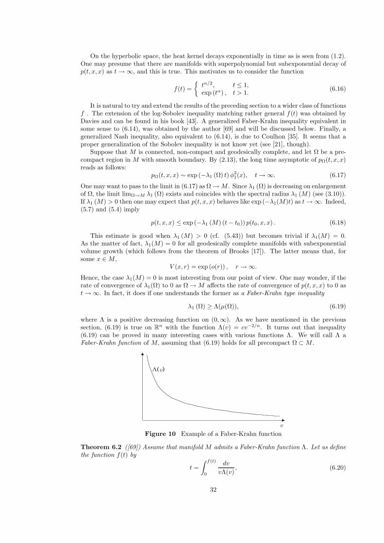
where Λ is a positive decreasing function on (0,∞). As we have mentioned in the previoussection, (6.19) is true on Rn with the function Λ(v) = cv−2/n. It turns out that inequality(6.19) can be proved in many interesting cases with various functions Λ. We will call Λ aFaber-Krahn function of M, assuming that (6.19) holds for all precompact Ω ⊂M .

( )

Figure 10 Example of a Faber-Krahn function

Theorem 6.2 ([69]) Assume that manifold M admits a Faber-Krahn function Λ. Let us definethe function f(t) by

t =∫ f(t)

0

dv

vΛ(v), (6.20)

32

assuming the convergence of the integral in (6.20) at 0. Then, for all t > 0, x ∈M , and ε > 0,

p(t, x, x) ≤ 2ε−1

f((1 − ε) t). (6.21)

Examples: 1. If Λ(v) = cv−2/n then (6.20) yields f(t) = c′tn/2. Hence, (6.21) amounts to(6.2).

2. Let

Λ(v) v−2/n, v ≤ 1,v−2/m, v > 1.

(6.22)

For example, the manifold M = K × Rm, where K is a compact manifold of the dimensionn−m, admits the Faber-Krahn function (6.22) (see Section 7.5). Then (6.20) gives

f(t) tn/2, t ≤ 1,tm/2, t > 1,

andsupxp(t, x, x) ≤ c

tm/2, ∀t > 1.

3. AssumeΛ(v) log−α v, v > 2,

and Λ(v) v−2/n for v < 2 (see Section 7.6 for examples of manifolds with this Λ). Then, forlarge t,

f(t) c1 exp(c2t

11+α

)and

supxp(t, x, x) ≤ C exp

(−ct 1

1+α

).

4. Let us takeΛ(v) ≡ λ1(M), v > 1,

and Λ(v) v−2/n for v < 1 (note that the constant function Λ(v) ≡ λ1(M) satisfies (6.19) butthe integral (6.20) diverges, so we have to modify it near v = 0). Then, for large t,

f(t) exp (λ1(M)t)

andsupxp(t, x, x) ≤ C exp (− (λ1(M) − ε) t) .

In fact, in this case ε can be taken 0 (this can be seen from the proof below or from (6.18)).Proof of Theorem 6.2. Fix a point y ∈M . We will prove that, for any precompact open setΩ with smooth boundary,

pΩ(t, y, y) ≤ Cεf((1 − ε) t)

,

provided y ∈ Ω. Let us start as in the proof of Theorem 6.1: denote u(t, x) = pΩ(t, x, y),

J(t) :=∫

Ω

u2(t, x)dµ(x)

and obtainJ ′(t) = −2

∫Ω

|∇u|2 dµ. (6.23)

Next, we have to estimate∫ |∇u|2 dµ from below via

∫u2dµ. The simplest way to do so is by

using the variational property of the first eigenvalue which gives∫Ω

|∇u|2 dµ ≥ λ1 (Ω)∫

Ω

u2dµ ≥ Λ(µ(Ω))∫

Ω

u2dµ.

However, this is not suitable for us because the resulting estimate of u will depend on Ω. Thefollowing lemma provides a more sophisticated way of applying (6.19).

33

Lemma 6.3 Assuming that (6.19) holds, we have, for any non-negative function u ∈ C2(Ω) ∩C(Ω)

vanishing on ∂Ω,

∫|∇u|2 ≥ (1 − ε)

(∫u2

)Λ

(2ε

(∫u)2∫u2

), (6.24)

for any ε ∈ (0, 1).

Remark 6.4 If Λ(v) = cv−2/n then (6.24) becomes the Nash inequality (6.8). Hence, (6.24)can be considered as a generalized Nash inequality.

Proof. The proof follows the argument of Gushchin [80]. Denote for simplicity A =∫udµ and

B =∫u2dµ. For any positive s, we have the obvious inequality

u2 ≤ (u− s)2+ + 2su,

which implies, by integration,

B ≤∫

u>s

(u− s)2dµ+ 2sA. (6.25)

Applying the Faber-Krahn inequality (6.19) in the region Ωs := u > s (observe that u − svanishes on the boundary ∂Ωs), we get

∫Ωs

(u − s)2dµ ≤∫Ωs

|∇u|2 dµΛ (µ(Ωs))

. (6.26)

s=u>s

s

0

u(x)

Figure 11 Applying a Faber-Krahn inequality for the region Ωs

Unlike Ω, the region Ωs admits estimating of its volume via the function u, as follows

µ(Ωs) ≤ 1s

∫Ω

u dµ = s−1A.

Hence, (6.25) and (6.26) imply

B ≤∫Ωs

|∇u|2 dµΛ (s−1A)

+ 2sA

whence ∫Ω

|∇u|2 dµ ≥ (B − 2sA) Λ(s−1A

).

Taking here s = εB2A , we finish the proof.

Applying Lemma 6.3 to estimate the right hand side of (6.23) and taking into account that∫u(t, x)dµ(x) ≤ 1,

34

we obtain

J ′ ≤ −2 (1 − ε) JΛ(

2ε

1J

).

Dividing this inequality by the right hand side, integrating it against dt from 0 to t and changingthe variables v = 2ε−1J−1, we obtain

∫ 2ε−1J−1

0

dv

vΛ(v)≥ 2 (1 − ε) t

whence, by the definition (6.20) of function f ,

J(t) ≤ 2ε−1

f(2(1 − ε)t).

We are left to notice that J(t) = pΩ (2t, y, y), and (6.21) follows.If the function Λ satisfying the hypotheses of Theorem 6.2 is continuous then f(t) ∈ C1(R+)

and

f ′ > 0, f(0) = 0, f(∞) = ∞ andf ′

fis non-increasing. (6.27)

Conversely, if f ∈ C1 (R+) satisfies (6.27) then Λ from (6.20) can be recovered by

Λ(f(t)) =f ′

f. (6.28)

The following Theorem is almost converse to Theorem 6.2.

Theorem 6.5 ([69]) Let the heat kernel on the manifold M admit the following estimate

supxp(t, x, x) ≤ 1

f(t), ∀t > 0, (6.29)

where f ∈ C1 (R+) satisfies (6.27) and certain regularity condition below. Then M admits theFaber-Krahn function cΛ(v) where Λ is defined by (6.28).

Moreover, for any precompact region Ω ⊂M and any integer k ≥ 1,

λk(Ω) ≥ cΛ(µ (Ω)k

). (6.30)

We say that a function g(t) has at most polynomial decay if, for some α > 0 and a ∈ [1, 2],

g(at) ≥ αg(t), ∀t > 0. (6.31)

The the regularity condition in the statement of Theorem 6.5 is as follows: the function g :=(log f)′ has at most polynomial decay. For example, the latter holds if, for some large A > 0,

f ′′

f ′ ≥ f ′

f− A

t.

All examples of f considered above, satisfy this condition. On the contrary, f(t) = 1−e−t doesnot satisfy it.Proof. The hypotheses (6.29) implies pΩ(t, x, x) ≤ 1

f(t) whence

∫Ω

pΩ(t, x, x)dµ(x) ≤ µ(Ω)f(t)

.

On the other hand, by the eigenfunction expansion (2.9),∫Ω

pΩ(t, x, x)dµ(x) =∫

Ω

∞∑i=1

e−λi(Ω)tφ2i (x)dµ(x) =

∞∑i=1

e−λi(Ω)t.

35

The right hand side here is bounded from below by ke−λk(Ω)t, whence

µ(Ω)f(t)

≥ ke−λk(Ω)t

andλk(Ω) ≥ 1

tlog

kf(t)µ(Ω)

. (6.32)

This inequality holds for all t > 0 so that we can choose t. Let us find t from the equation

f(t/2) = µ(Ω)/k.

For this t, we obtain from (6.32)

λk(Ω) ≥ 1t

(log f(t) − log f(t/2)) =12g(θ),

where g := (log f)′ and θ ∈ (t/2, t). By the regularity condition (6.31), we have g(θ) ≥ αg(t/2).Finally, we apply (6.28):

g(t/2) =f ′(t/2)f(t/2)

= Λ (f(t/2)) = Λ(µ(Ω)k

)

whence

λk(Ω) ≥ α

2Λ(µ(Ω)k

),

which was to be proved.It is follows from Theorems 6.2 and 6.5 that the heat kernel upper bound (6.29) is equiv-

alent to the certain Faber-Krahn type inequality, up to some constant multiples. Clearly, thegeneralized Nash inequality (6.24) involved in the proof of Theorem 6.2, is also equivalent toeach of these hypotheses. The latter was further developed in an abstract semigroup setting byCoulhon [35]. He also gave another proof of the first part of Theorem 6.5 avoiding usage of theeigenfunction expansion.

Putting together Theorems 6.2 and 6.5, we obtain

Corollary 6.6 Suppose that the function Λ satisfies the hypotheses of Theorems 6.2 and 6.5.If, for any precompact open set Ω ⊂M ,

λ1(Ω) ≥ Λ(µ(Ω)) (6.33)

then, for all integers k ≥ 1,λk(Ω) ≥ cΛ(Cµ(Ω)). (6.34)

For example, for the Euclidean function Λ(v) = cv−2/n, we obtain

λk(Ω) ≥ c′(

k

µ(Ω)

)2/n

.

Note that (6.34) does not follow from (6.33) for an individual set Ω: it is essential that (6.33)holds for all Ω.

By reverting the Faber-Krahn inequality (6.33), it is possible to prove some lower boundsof the heat kernel - see [36, Theorem 3.2].

36

6.3 Localized upper estimate

We consider here the localized version of Theorem 6.1.

Theorem 6.7 ([66], [69]) Suppose that, for some x ∈M and r > 0, the following Faber-Krahninequality holds: for any precompact open set Ω ⊂ B(x, r)

λ1(Ω) ≥ aµ (Ω)−2/n, (6.35)

where a > 0 and n > 0. Then, for any t > 0,

p(t, x, x) ≤ Ca−n/2

min(t, r2)n/2, (6.36)

where C = C(n).

Remark 6.8 This theorem contains Theorem 6.1 as r → ∞, taking into account that (6.35)is equivalent to (6.3). However, the method of proof of Theorems 6.1 and 6.2 does not work inthe setting of Theorem 6.7 because it requires (6.35) for all Ω, not only for those in B(x, r).

The coefficient a in (6.36) can be absorbed into the constant C. However, by varying theball B(x, r), we may have different a for different balls so that the exact dependence on a in(6.36) may be crucial. In the next section we will consider a setting where a depends explicitlyon B(x, r).

Proof. We start with the following mean-value type inequality.

Lemma 6.9 Suppose that the Faber-Krahn inequality (6.35) holds for any precompact open setΩ ⊂ B(x, r). Then, for any τ ∈ (0, r2], t ≥ τ and for any positive solution u of the heat equationin the cylinder (t− τ, t] ×B(x,

√τ), we have

u(t, x) ≤ Ca−n/2

τ1+n/2

t∫t−τ

∫B(x,

√τ)

u(s, y)dµ(y)ds, (6.37)

where C = C(n).

Remark 6.10 The term τ1+n/2 is proportional to the volume of the cylinder of the height τand of the base being a ball of radius

√τ in Rn. This reflects the fact that the Faber-Krahn

inequality (6.35) is optimal in Rn but may not be optimal in M . A different type of the mean-value property (5.17) related to the volume V (x,

√τ ) on M was considered in Section 5.2 (see

also the next section).

The proof of (6.37) consists of two steps. The first step is the L2-mean-value inequality,that is, (6.37) for u2 instead of u, which was proved in [67, Theorem 3.1]. Alternatively, theL2-mean-value inequality follows from the first part of the Moser iteration argument [106], giventhe equivalence of (6.35) and certain Sobolev inequality (see [20]). The second step is to derive(6.37) from the L2-mean-value inequality. This is done by using the argument of Li and Schoen[95] (see also [97] and [37]).

The estimate (6.36) follows from Lemma 6.9 similarly to the first part of the proof ofTheorem 5.8. Indeed, integrating in time the inequality∫

M

p(s, x, y)dµ(y) ≤ 1

we obtain, for all t ≥ τ > 0, ∫ t

t−τ

∫M

p(s, x, y)dµ(y) ≤ τ .

37

Hence (6.37) yields, for u = p(·, x, ·) and for τ ∈ (0, r2],

p(t, x, x) ≤ Ca−n/2

τ1+n/2

∫ t

t−τ

∫M

p(s, x, y)dµ(y) ≤ Ca−n/2

τn/2.

Clearly, (6.36) follows if we choose τ = min(t, r2).

Corollary 6.11 Suppose that, for all x ∈ M and some r > 0, the Faber-Krahn inequality(6.35) holds, for any precompact open set Ω ⊂ B(x, r). Then, for any D > 2 and all x, y ∈M ,t > 0,

p(t, x, y) ≤ Ca−n/2

min(t, r2)n/2exp

(−d

2(x, y)2Dt

), (6.38)

where C = C(n,D).

The estimate (6.38) follows from (6.36) and from the inequality (5.14) of Corollary 5.5. Ifwe use (5.15) instead of (5.14) then we obtain

p(t, x, y) ≤ Ca−n/2eλ1(M)t0

min(t, t0)n/2exp

(−λ1(M)t− d2(x, y)

2Dt

)(6.39)

where t0 = r2. By absorbing a and t0 into C, we can rewrite (6.39) as follows:

p(t, x, y) ≤ C′

min(t, 1)n/2exp

(−λ1(M)t− d2(x, y)

2Dt

). (6.40)

6.4 Relative Faber-Krahn inequality and the decay of the heat kernelas V (x,

√t)−1.

We return here to heat kernel upper bound

p(t, x, x) ≤ C

V (x,√t), (6.41)

which was discussed already in Section 5.17. Similarly to the equivalence

On-diagonal bound (6.2)⇐⇒Faber-Krahn inequality (6.11)

mentioned in Section 6.1, we will show that (6.41) is “almost” equivalent to the relative Faber-Krahn inequality defined as follows.

Definition 6.12 We say that M admits the relative Faber-Krahn inequality if, for any ballB(x, r) ⊂M and for any precompact open set Ω ⊂ B(x, r),

λ1(Ω) ≥ b

r2

(V (x, r)µ(Ω)

)ν, (6.42)

with some positive constants b, ν.

B(x,R)

Ω

Figure 12 Subset Ω of the ball B(x,R)

38

It is easy to see that (6.42) holds in Rn with ν = 2/n. It is possible to prove that therelative Faber-Krahn inequality holds on any geodesically complete manifold of non-negativeRicci curvature - see [67]. In general, a non-negatively curved manifold admits no uniformFaber-Krahn function in the spirit of Section 6.2. The inequality (6.42) was designed to over-come this difficulty. It provides a lower bound for λ1 (Ω), which takes into account not onlyvolume µ(Ω) but also location of the set Ω, via the ball B(x, r).

We say that the volume function V (x, r) satisfies the doubling property if, for some constantC,

V (x, 2r) ≤ CV (x, r), ∀x ∈M, r > 0. (6.43)Now we can state the main theorem of this section.

Theorem 6.13 ([69, Proposition 5.2]) Let M be a geodesically complete manifold.If M admits the relative Faber-Krahn inequality then the heat kernel satisfies the upper bound

(6.41), for all x ∈M and t > 0, and the volume function V (x, r) satisfies the doubling property(6.43).

Conversely, the heat kernel upper bound (6.41) and the doubling volume property (6.43)imply (6.42).

Proof. The implication (6.42)=⇒(6.41) follows from Theorem 6.7. Indeed, given a ball B(x, r),we have, by (6.35), for any precompact open set Ω ⊂ B(x, r),

λ1 (Ω) ≥ aµ(Ω)−2/n, (6.44)

where n = 2/ν and

a =b

r2V (x, r)2/n. (6.45)

Hence, Theorem 6.7 implies, for any r > 0,

p(t, x, x) ≤ Ca−n/2

min(t, r2)n/2.

Taking r =√t and substituting a from (6.45) we obtain (6.41).

Another proof of (6.42)=⇒(6.41) follows by Theorem 5.8. Indeed, given (6.44), Lemma 6.9implies that, for any positive solution u of the heat equation in the cylinder (t− r2, t]×B(x, r)(assuming τ := r2 ≤ t),

u(t, x) ≤ Ca−n/2

r2+n

t∫t−r2

∫B(x,r)

u(s, y)dµ(y)ds.

Substituting a from (6.45), we obtain the mean-value property (MV) (see Definition 5.7). Hence,Theorem 5.8 can be applied and yields (6.41).

The implication (6.42)=⇒(6.43) is proved by the argument of Carron [20] - see [69, p.442].The second part of Theorem 6.13 – the implication (6.41)+(6.43)=⇒(6.42), is proved similarlyto Theorem 6.5 - see [69, p.443].

The above proof together with Theorems 5.8 and 5.12 gives the following

Corollary 6.14 The following implications hold

Relative Faber-Krahn inequality (6.42)

Mean-value property (MV) and volume doubling (6.43).

Gaussian upper bound (5.19) and volume doubling (6.43)

On-diagonal upper bound (6.41) and volume doubling (6.43)⇓

On-diagonal lower bound (5.40)

39

Another (direct) proof of the second equivalence was obtained by Li and Wang [97].

7 Isoperimetric inequalities

7.1 Isoperimetric inequalities and λ1(Ω)

Isoperimetric inequality relates the boundary area of regions to their volume. We say thatmanifold M admits the isoperimetric function I if, for any precompact open set Ω ⊂ M withsmooth boundary,

σ (∂Ω) ≥ I (|Ω|) , (7.1)

where|Ω| := µ (Ω) .

For example, Rn admits the isoperimetric function I(v) = cnvn−1

n . Indeed, let Ω∗ ⊂ Rn bea ball of the same volume as Ω and let r be its radius. Then, by the classical isoperimetricinequality,

σ (∂Ω) ≥ σ (∂Ω∗) = ωnrn−1 = cn

(ωnnrn)n−1

n

= c |Ω∗|n−1n = cn |Ω|n−1

n .

Other examples of isoperimetric functions will be shown below.It turns out that the isoperimetric inequality (7.1) implies a Faber-Krahn inequality (6.19).

The next statement is a version of Cheeger’s inequality [26].

Proposition 7.1 Let I(v) be a non-negative continuous function on R+ such that I(v)/v isnon-increasing. Assume that M admits the isoperimetric function I. Then M admits theFaber-Krahn function

Λ (v) :=14

(I (v)v

)2

. (7.2)

For example, if I(v) = cvn−1

n then (7.2) yields Λ(v) = c2

4 v−2/n.

Proof. Given a non-negative function f ∈ C∞0 (Ω), we denote

Ωs = x : f(x) > s .

By Sard’s theorem, the boundary ∂Ωs is smooth, for almost all s, so that we can apply theisoperimetric inequality (7.1) for Ωs and obtain

σ(∂Ωs) ≥ I(|Ωs|) (7.3)

for almost all s. Next, we use the co-area formula∫M

|∇f | dµ =∫ ∞

0

σ (∂Ωs) ds , (7.4)

which implies with (7.3) and the non-increasing of I(v)/v,∫M

|∇f | dµ ≥∫ ∞

0

I(|Ωs|)ds

=∫ ∞

0

I(|Ωs|)|Ωs| |Ωs| ds

≥ I(|Ω|)|Ω|

∫ ∞

0

|Ωs| ds

=I(|Ω|)|Ω|

∫M

f dµ. (7.5)

40

By the Cauchy-Schwarz inequality, we have∫M

∣∣∇f2∣∣ dµ = 2

∫M

f |∇f | ≤ 2[∫

M

f 2 dµ

∫M

|∇f |2 dµ]1/2

. (7.6)

Applying (7.5) to f2 instead of f and by (7.6), we obtain

I(|Ω|)|Ω|

∫M

f 2 dµ ≤∫M

∣∣∇f2∣∣ dµ ≤ 2

[∫M

f 2 dµ

∫M

|∇f |2 dµ]1/2

whence (I(|Ω|)|Ω|

)2 ∫M

f 2 dµ ≤ 4∫M

|∇f |2 dµ

and

λ1 (Ω) ≥ 14

(I(|Ω|)|Ω|

)2

,

which was to be proved.Combining Proposition 7.1 with Theorem 6.2 and Corollary 5.5, we obtain

Corollary 7.2 Assume that manifold M admits a non-negative continuous isoperimetric func-tion I(v) such that I(v)/v is non-increasing. Let us define the function f(t) by

t = 4∫ f(t)

0

vdv

I2(v), (7.7)

assuming the convergence of the integral in (7.7) at 0. Then, for all x ∈M, t > 0 and ε > 0,

p(t, x, x) ≤ 2ε−1

f((1 − ε) t). (7.8)

Furthermore, if the function f satisfies in addition the regularity condition (5.11) then, for allx, y ∈M , t > 0, D > 2 and some ε > 0,

p(t, x, y) ≤ C

f(εt)exp

(−d

2(x, y)2Dt

). (7.9)

In the next sections, we will show examples of manifolds satisfying certain isoperimetric andFaber-Krahn inequalities where the heat kernel estimates given by Theorems 6.2, 6.7, 6.13 andCorollaries 6.11, 7.2 can be applied.

7.2 Isoperimetric inequalities and the distance function

Here we mention a certain method of proving isoperimetric inequalities, which was introducedby Michael and Simon [104]. Suppose that we have a distance function r(x, ξ) on M . This maybe the Riemannian distance or a general distance function satisfying the usual axioms of themetric space, in particular, the triangle inequality. We will denote r(x, ξ) by rξ(x) to emphasizethat it will be regarded as a function of x with a fixed (but arbitrary) ξ. It turns out that anisoperimetric inequality on M can be proved if one knows certain bounds for |∇rξ| and ∆rξ.

Theorem 7.3 (Michael–Simon [104], Chung–Grigor’yan–Yau [33]) Let M be a geodesicallycomplete Riemannian manifold of dimension n > 1. Suppose that rξ(x) is a distance functionon M such that, for all ξ, x ∈M ,

|∇rξ(x)| ≤ 1 (7.10)

and∆r2ξ (x) ≥ 2n (7.11)

(assuming that r2ξ ∈ C2(M)). Then M admits the isoperimetric function I(v) = cvn−1

n wherec = cn > 0.

41

Let us explain why (7.10) and (7.11) should be related to isoperimetric inequalities. Indeed,integrating (7.10) over a precompact region Ω ⊂M with smooth boundary and using the Greenformula (2.4), we obtain

2n |Ω| =∫

Ω

∆(r2ξ )dµ = 2∫∂Ω

rξ∂rξ∂ν

dσ , (7.12)

where ν is the outward normal vector field on ∂Ω. With the obvious inequality ∂rξ

∂ν ≤ |∇rξ| ≤ 1,(7.12) implies

n |Ω| ≤(

supΩrξ

)σ(∂Ω). (7.13)

This is already a weak form of isoperimetric inequality. A certain argument allows to extend(7.13) as to show the isoperimetric inequality

σ (∂Ω) ≥ c |Ω|n−1n .

See [104] or [33] for further details.

7.3 Minimal submanifolds

Let M be an n-dimensional submanifold of RN with the Riemannian metric inherited from RN .SubmanifoldM is called minimal if its normal mean curvature vectorH(x) = (H1(x), H2(x), ..., HN (x))vanishes for all x ∈M (see [113]). It turns out that already the minimality of M implies certainisoperimetric property.

Theorem 7.4 (Bombieri – de Giorgi – Miranda [16]) Any n-dimensional minimal submanifoldM admits the isoperimetric function I(v) = cv

n−1n , c > 0.

Proof. Consider the coordinate functions Xi in RN as functions on M . Then ∆Xi = Hi(x)where ∆ is the Laplacian on M (see [113, Theorem 2.4]). Let us denote by rξ(x) the (extrinsic)Euclidean distance in RN between the points x, ξ ∈M . Shifting the coordinates X1, X2, ..., XN

in RN to have the origin ξ, we have

∆r2ξ =N∑i=1

∆(X2i ) = 2

N∑i=1

XiHi + 2N∑i=1

|∇Xi|2 .

The term∑XiHi identically vanishes if M is minimal. The sum

∑Ni=1 |∇Xi|2 is equal to n

for any n-dimensional submanifold, which can be verified by a direct computation. Hence, weconclude

∆r2ξ = 2n. (7.14)

On the other hand, it is obvious that |∇rξ| ≤ 1 because the extrinsic distance is majorized bythe intrinsic Riemannian distance on M . Hence, we can apply Theorem 7.3 and conclude theproof.

Theorem 7.4 and Corollary 7.2 imply the following uniform upper bound for the heat kernelon M

p(t, x, y) ≤ C

tn/2exp

(−d

2(x, y)2Dt

). (7.15)

7.4 Cartan-Hadamard manifolds

A manifold M is called a Cartan-Hadamard manifold if M is geodesically complete simply con-nected non-compact Riemannian manifold with non-positive sectional curvature. For example,Rn and Hn are Cartan-Hadamard manifolds.

42

Theorem 7.5 (Hoffman – Spruck [84]) Any Cartan-Hadamard manifold M of the dimensionn admits the isoperimetric function I(v) = cv

n−1n , c > 0.

This theorem can also be derived from Theorem 7.3. Indeed, denote by rξ(x) the geodesicdistance between the point x and ξ on M . If M = Rn then ∆r2ξ = 2n. For general Cartan-Hadamard manifold, the comparison theorem for the Laplacian implies ∆r2ξ ≥ 2n (see [122]),whereas |∇rξ| ≤ 1 holds on any manifold.

Hence, the heat kernel estimate (7.15) is valid on Cartan-Hadamard manifolds, too. On theother hand, by Proposition 7.1, Cartan-Hadamard manifolds satisfy the hypotheses of Corollary6.11. Therefore, (6.40) holds, that is,

p(t, x, y) ≤ C

min(1, tn/2

) exp(−λ1(M)t− d2(x, y)

2Dt

), (7.16)

which can be better than (7.15) if λ1(M) > 0.McKean’s theorem [103] says that if the sectional curvature of the Cartan-Hadamard man-

ifold is bounded from above by −K2 then

λ1 (M) ≥ (n− 1)2

4K2 . (7.17)

Indeed, consider again the Riemannian distance function rξ(x) . As Yau [139] showed, on suchmanifolds

∆rξ ≥ (n− 1)K, (7.18)

away from ξ. Given a precompact open set Ω ⊂ M with smooth boundary, we choose ξ /∈ Ωand integrate (7.18) over Ω. By the Green formula 2.4, we obtain∫

∂Ω

∂rξ∂ν

dσ ≥ (n− 1)K |Ω| .

Since ∂rξ

∂ν ≤ |∇rξ| ≤ 1, we arrive to the isoperimetric inequality

σ (∂Ω) ≥ (n− 1)K |Ω| ,

whence (7.17) follows by Proposition 7.1.Hence, (7.16) implies, for all x, y ∈M , t > 0 and D > 2,

p(t, x, y) ≤ C

min(1, tn/2)exp

(− (n− 1)2

4K2t− d2(x, y)

2Dt

). (7.19)

Let us compare (7.19) with the sharp uniform estimate of the heat kernel on the hyperbolicspace Hn

K of the constant negative curvature −K2 obtained by Davies and Mandouvalos [50]:

p(t, x, y) (1 + d+ t)n−3

2 (1 + d)tn/2

exp(− (n− 1)2

4K2t− d2

4t− n− 1

2Kd

), (7.20)

where d = d(x, y) (see [43] and [77] for the exact formula for the heat kernel on hyperbolicspaces; the estimate (7.20) admits a far reaching generalization for symmetric spaces - see [3]).

If t→ ∞ then (7.20) yields

p(t, x, x) t−3/2 exp(− (n− 1)2

4K2t

),

which is better than (7.19) by the factor t−3/2. The geometric nature of this factor is stillunclear.

43

Another difference between (7.19) and (7.20) is the constant D > 2 in the Gaussian term. Itis possible to put D = 2 in (7.19) at expense of the polynomial correction term, as in Theorem5.9 – see [68, p.254] or [69, Theorem 5.2].

Yet another difference between (7.19) and (7.20) is the third term n−12 Kd in the exponential.

It does not play a significant role for the heat kernel in the hyperbolic space because it isdominated by the sum of two other terms in the exponential (7.20). However, it is possible tointroduce a similar term for general Cartan-Hadamard manifolds, and it may be leading if thecurvature goes to −∞ fast enough as x→ ∞.

Fix a point o ∈M and denote3

L(r) := λ1(M \B(o, r)). (7.21)

Clearly, L(r) is increasing in r and L(0) = λ1(M). If the sectional curvature outside the ballB(o, r) is bounded above by −K2(r) (whereK(r) is positive and increasing) then a modificationof (7.17) says that

L(r) ≥ (n− 1)2

4K(r)2. (7.22)

Theorem 7.6 ([69, Theorem 5.3]) Let M be a Cartan-Hadamard manifold of the dimensionn and o ∈M. Then, for all t > 0, x ∈M \B(o,

√t), c ∈ (0, 1) and some ε = ε(c) > 0,

p(t, o, x) ≤ C

tn/2exp

(−cλ1(M)t− c

d2

4t− εd

√L(cd)

), (7.23)

where d = dist(o, x) and C = C(c, n).

Proof of Theorem 7.6 is similar to that of Theorem 6.7 but uses a more general mean-valuetype inequality than Lemma 6.9 – see [69] for details. It is not clear whether one can put c = 1here.

As a consequence we see that if the sectional curvature outside the ball B(o, r) is boundedabove by −K2(r) then (7.23) and (7.22) yield

p(t, o, x) ≤ C

tn/2exp

(−cλ1(M)t− c

d2

4t− εK(cd)d

). (7.24)

In particular, if K(r) r then the term K(cd)d is leading as d→ ∞.It is possible to prove the following matching lower bound. Assume that the sectional

curvature inside the ball B(o, r) is bounded below by −K2(r). Then we claim that, for allt > 0, x ∈M and ε > 0,

p(t, o, x) ≥ c

tn/2exp

(− (λ1(M) + ε) t− C

d2

4t− CK(d+ C)d

), (7.25)

where c = c(o, ε) > 0 (cf. (7.28) below).Comparison of (7.24) and (7.25) shows that there is a big gap in the values of the constants

in the upper and lower bounds. The problem of obtaining optimal heat kernel estimates whenthe curvature grows to −∞ faster than quadratically in r, is not well understood.

Another interesting consequence of (7.23) is related to the essential spectrum of the operator∆M . Denote by λess(M) the bottom of the essential spectrum of −∆M in L2(M,µ). It is knownand is due to Donnelly [58] that, on any complete manifold,

λess(M) = limr→∞L(r) , (7.26)

where L(r) is defined by (7.21). It is possible to derive from (7.23) and (7.26) that

lim supd→∞

1d

supt>0

log p(t, o, x) ≤ −C(√

λ1(M) +√λess(M)

), (7.27)

3The notation λ1(Ω) (where Ω is not necessarily compact) is defined by (6.12). This is the bottom of thespectrum of the operator −∆Ω in L2(Ω, µ).

44

where d = d(x, o) (see [69, Corollary 5.1]) and C > 0 is an absolute constant. It would beinteresting to understand to what extent this inequality is sharp, in particular, what is a sharpvalue of C. For the hyperbolic space, equality is attained in (7.27) with C = 1.

7.5 Manifolds of bounded geometry

We say that a manifold M has bounded geometry if its Ricci curvature is uniformly boundedbelow and if its injectivity radius is bounded away from 0. The hypothesis of bounded geometryimplies that, for some r0 > 0, all balls B(x, r0), x ∈ M , are uniformly quasi-isometric to theEuclidean ball BE(r0) ⊂ Rn, where n = dimM . The term “quasi-isometric” means that thereis a diffeomorphism between B(x, r0) and BE(r0) which changes the distances at most by aconstant factor, and the word “uniform” refers to the fact that this constant factor is the samefor all x ∈M .

In other words, the manifold M looks like being patched from slightly distorted copies ofthe ball BE(r0). Clearly, a manifold of bounded geometry is geodesically complete.

n

M

B(x, r0)

BE(r0)

Figure 13 Manifold of bounded geometry is “patched” from slightly distorted Euclideanballs

The hypotheses of Corollary 6.11 are satisfied on the manifold M of bounded geometry.Hence, the upper bound (6.40) (the same as (7.16)) holds on M . Using Proposition 5.14 andthe standard chain argument with the local Harnack inequality, it is possible to prove thefollowing lower bound

p(t, x, y) ≥ cx,ε exp(−(λ1(M) + ε)t− C

d2(x, y)t

), (7.28)

for any ε > 0 and all t > 0, x, y ∈ M . Hence, if λ1(M) > 0 then (6.40) provides a correct rateof decay of p(t, x, y) as t→ ∞ and as y → ∞.

It turns out that even in the case λ1(M) = 0, there is a priori rate of decay of the heatkernel as t→ ∞. This is based on the following isoperimetric property of manifolds of boundedgeometry.

Theorem 7.7 Any n-dimensional manifold of bounded geometry admits the following isoperi-metric function, for some c > 0,

I(v) = cmin(v

n−1n , 1

). (7.29)

The meaning of (7.29) is the following. For small v, the function I(v) is nearly the Euclideanone which corresponds to the fact that the small scale geometry of M is uniformly quasi-isometric to that of Rn. For large v, (7.29) gives I(v) = c, which is attained on the cylinderM = Rn−1 × S1 (see Fig. 14). Roughly speaking, (7.29) says that a manifold of boundedgeometry expands at ∞ at least as fast as a cylinder.

45

Ω

Figure 14 The surface area of ∂Ω does not increase when the set Ω ⊂ Rn−1 × S1 isstretching.

Proof. We need to show that, for any precompact open set Ω with smooth boundary,

σ (∂Ω) ≥ I(|Ω|).

CASE 1. Assume that, for any x ∈ M , the set Ω covers less than a half of the volume ofthe ball B(x, r0/3). Then, for any point x ∈ Ω, there exists a positive number r(x) ≤ r0/3 suchthat

14≤ σ(∂Ω ∩B(x, r(x)))

V (x, r(x))≤ 1

2. (7.30)

All balls B(x, r(x)), x ∈ Ω, cover Ω. Choose a finite number of them also covering Ω. Then, byusing the Banach argument, choose out of them a finite family of disjoint balls B(xi, ri) (whereri = r(xi)) so that the concentric balls B(xi, 3ri) cover Ω.

B(xi, ri)

Figure 15 Set Ω (shaded) takes in each ball B(xi, ri) nearly one half of its volume, whereasthe balls B(xi, 3ri) cover all of Ω.

In particular, we have ∑i

V (xi, 3ri) ≥ |Ω| . (7.31)

On the other hand, we use the following isoperimetric property of partitions of balls.

Proposition 7.8 For any smooth hypersurface Γ in B(x, r) (where r ≤ r0) dividing B(x, r)into two open subsets each having volume at least v,

σ(Γ) ≥ cvn−1

n . (7.32)

If B(x, r) is a Euclidean ball then (7.32) is a classical inequality, the best constant c inwhich was found by Maz’ya - see [102]. If B(x, r) is a ball on manifold of bounded geometryand r ≤ r0 then (7.32) follows from its Euclidean version and from the fact that the measuresof all dimensions in B(x, r0) differ from their Euclidean counterparts at most by a constantfactor.

Applying (7.32) to Γ = ∂Ω ∩B(xi, ri) and using (7.30), we obtain

σ (∂Ω ∩B(xi, ri)) ≥ cV (xi, ri)n−1

n .

Adding up these inequalities over all i and applying the elementary inequality

∑i

aνi ≥(∑

i

ai

)ν

, (7.33)

46

which is valid for ai ≥ 0 and 0 ≤ ν ≤ 1, we obtain

σ(∂Ω) ≥ c

(∑i

V (xi, ri)

)n−1n

. (7.34)

Finally, we use V (x, 3r) ≤ CV (x, r), which is true for all r ≤ r0/3. Therefore, (7.31) and(7.34) imply

σ(∂Ω) ≥ c |Ω|n−1n . (7.35)

which was to be proved.CASE 2. Assume that, for some x ∈ M , the set Ω covers at least a half of the volume of

the ball B(x, r0/3). By moving the point x away, we may assume that

|Ω ∩B(x, r0/3)| =12V (x, r0/3). (7.36)

ΩB(x,r0/3)

Figure 16 Set Ω covers exactly one half of the volume of the ball B(x, r0/3).

By Proposition 7.8 and (7.36), we have

σ (∂Ω) ≥ σ (∂Ω ∩B(x, r0/3)) ≥ cV (x, r0/3)n−1

n ≥ const, (7.37)

which together with (7.35) finishes the proof.Theorem 7.7 and Corollary 7.2 imply

Theorem 7.9 On any manifold of bounded geometry,

p(t, x, x) ≤ Cmax(t−n/2, t−1/2

),

for all x ∈M and t > 0. In particular, for all x ∈M and t > 1,

p(t, x, x) ≤ Ct−1/2. (7.38)

The exponent 12 in (7.38) is sharp as is shown by (2.24) for the manifold M = S1 × Rn−1.

The estimate (7.38) was proved by different methods by Varopoulos [132], Chavel and Feldman[25], Coulhon and Saloff-Coste [39], [34], Grigor’yan [70].

Sharper estimates of the heat kernel can be obtained assuming a modified isoperimetricinequality on M . Let us say that M admits a modified isoperimetric function I(v) if σ (∂Ω) ≥I(|Ω|), for all precompact regions Ω ⊂M with smooth boundary such that Ω contains a ball ofthe radius r0. The purpose of this notion introduced by Chavel and Feldman [25] is to separatethe large scale isoperimetric properties of the manifold from its local properties. For example,the Riemannian product M = K × Rm where K is a compact manifold of the dimensionn − m, admits the modified isoperimetric function I(v) = cv

m−1m (see [64]). As follows from

Theorem 7.7, every manifold of bounded geometry admits the modified isoperimetric functionI(v) = const.

Theorem 7.10 (Chavel – Feldman [25]) If M is a manifold of bounded geometry admittingthe modified isoperimetric function I(v) = cv

m−1m then, for all x ∈M and t > 1,

p(t, x, x) ≤ Ct−m/2 .

47

Proof. It suffices to verify that M admits the following (not modified!) isoperimetric function

v → c′

vn−1

n , v ≤ 1,v

m−1m , v ≥ 1.

The proof of that follows the same line of reasoning as the proof of Theorem 7.7, with thefollowing modification. No change is required for Case 1. In Case 2, take again the point x forwhich (7.36) is satisfied and consider the region Ω0 = Ω ∪B(x, r0). Since Ω0 contains a ball ofradius r0, the modified isoperimetric inequality gives

σ(∂Ω0) ≥ c |Ω0|m−1

m ≥ c |Ω|m−1m .

B(x,r0) 0= B(x,r0)

B(x,r0)

B(x,r0/3)

Figure 17 Sets Ω and Ω0

To finish the proof, it suffices to show

σ(∂Ω0) ≤ Cσ(∂Ω). (7.39)

The idea is that by adding the ball to Ω, we do not increase considerably the surface area of ∂Ωbecause the part of ∂Ω covered by the ball is comparable to the boundary of the ball. Formally,we write

σ(∂Ω0) ≤ σ(∂Ω) + σ(∂B(x, r0))≤ σ(∂Ω) + Crn−1

0 . (7.40)

On the other hand, as follows from (7.37),

σ(∂Ω ∩B(x, r0)) ≥ crn−10 .

We see that the first term dominates in (7.40) whence (7.39) follows.See [70] for extension of Theorem 7.10 to a more general setup of manifolds of weak bounded

geometry.The following theorem improves (7.38) assuming the volume growth instead of an isoperi-

metric inequality.

Theorem 7.11 (Coulhon – Saloff-Coste [38]) Assume that M has bounded geometry and that

V (x, r) rN , ∀x ∈M, r > 1. (7.41)

Then, for all x ∈M and t > 1,p(t, x, x) ≤ Ct−

NN+1 . (7.42)

Note that 12 ≤ N

N+1 < 1 so that (7.42) is better than (7.38) whenever N > 1. The proofof Theorem 7.11 in [38, Theorem 8] contains implicitly the fact that the manifold in questionadmits the Faber-Krahn function

Λ(v) = c

v−2/n, v ≤ 1,v−

N+1N , v ≥ 1.

48

Given that much, Theorem 7.11 can be derived from Theorem 6.2. See [35] for further resultsin this direction.

Let us recall for comparison that Theorem 5.11 yields, under the hypotheses of Theorem7.11, the following lower bound, for all x ∈M and t large enough,

p(t, x, x) ≥ c

(t log t)N/2.

It seems that the entire range between these two extreme behaviors of the heat kernel given byt−

NN+1 and (t log t)−N/2, is actually possible.Any manifold M of bounded geometry has at most exponential volume growth, that is, for

all x ∈M and r > 1,V (x, r) ≤ C exp (Cr) .

This follows from the fact that M can be covered by a countable family of balls of radius r0/2,which has a uniformly finite multiplicity (see, for example, [87]). By Theorem 5.13, one obtainsthe heat kernel lower estimate, for all x ∈M and t ≥ t0,

p(t, x, x) ≥ c exp (−Kt) ,

for some c > 0 and K > 0. By the chain argument involving the local Harnack inequality, thisestimate can be extended to

p(t, x, y) ≥ c exp(−Kt− C

d2(x, y)t

), (7.43)

for all x, y ∈ M and t ≥ t0. The difference between (7.28) and (7.43) is that the former is notuniform with respect to x. On the other hand, (7.28) provides the sharp rate e−λ1(M)t of theheat kernel decay as t→ ∞ whereas the constant K is (7.43) may be much larger than λ1(M)- see [126].

7.6 Covering manifolds

Let Γ be a discrete group of isometries of the manifold M . We say that the manifold M is aregular cover of the manifold K with the deck transformation group Γ if K is isometric to thequotient MΓ. Intuitively, one can imagine M as a manifold glued from many copies of Kmoving from one to another by using the group action of Γ.

K

M

M/

= 2

Figure 18 Manifold M covers K by the group Γ = Z2

49

If M is a regular cover of a compact manifold K then M has bounded geometry so thatthe results of the previous section apply. However, much more can be said about the heatkernel given the volume growth of M . The following isoperimetric inequality of Coulhon andSaloff-Coste plays the crucial role.

Theorem 7.12 (Coulhon – Saloff-Coste [38, Theorem 4]) Let a non-compact manifold M bea regular cover of a compact manifold K. Let V(r) be a positive increasing function on R+

possessing certain regularity and such that, for some (fixed) o ∈M and all r > 0,

V (o, r) ≥ V(r). (7.44)

Then, for some (large) constant C > 0, the manifold M admits the isoperimetric function

I(v) :=v

CV−1(Cv), (7.45)

where V−1 is the inverse function.

Next theorem provides the heat kernel upper bound on covering manifolds.

Theorem 7.13 Referring to Theorem 7.12, we have, for all x ∈M , t > 0 and some ε > 0,

p(t, x, x) ≤ C

V(ρ(εt)), (7.46)

where ρ is defined by

t =∫ ρ(t)

0

r2d

drlogV(r) dr. (7.47)

Proof. Let us apply Corollary 7.2 with the isoperimetric function (7.45). Then the upperbound (7.8) holds with the function f defined by (7.7). Substituting (7.45) into (7.7), weobtain

t = 4C2

∫ f(t)

0

[V−1(Cv)]2dv

v

= 4C2

∫ Cf(t)

0

[V−1(v)]2dv

v

= 4C2

∫ V−1(Cf(t))

0

r2dV(r)V(r)

.

Setting c = 1/(4C2) and using the definition (7.47) of ρ, we obtain

V−1 (Cf(t)) = ρ (ct)

andf(t) = C−1V(ρ(ct)).

Hence, (7.46) follows from (7.8).For example, if V (o, r) ≥ crN then take V(r) = crN and, by (7.47), ρ(t) √

t. Hence,(7.46) implies p(t, x, x) ≤ Ct−N/2.

If V (o, r) ≥ exp (rα) =: V(r) (for large r) then we obtain ρ(t) t1

2+α and

p(t, x, x) ≤ C exp(−ct α

2+α), (7.48)

for large t. In the particular case α = 1, we have

p(t, x, x) ≤ C exp(−ct1/3

). (7.49)

It turns out that the exponent 1/3 here is sharp. Indeed, Alexopoulos [1] showed that a similaron-diagonal lower bound holds provided the deck transformation group Γ is polycyclic andV (o, r) exp (r). See [115] for further results of this type.

50

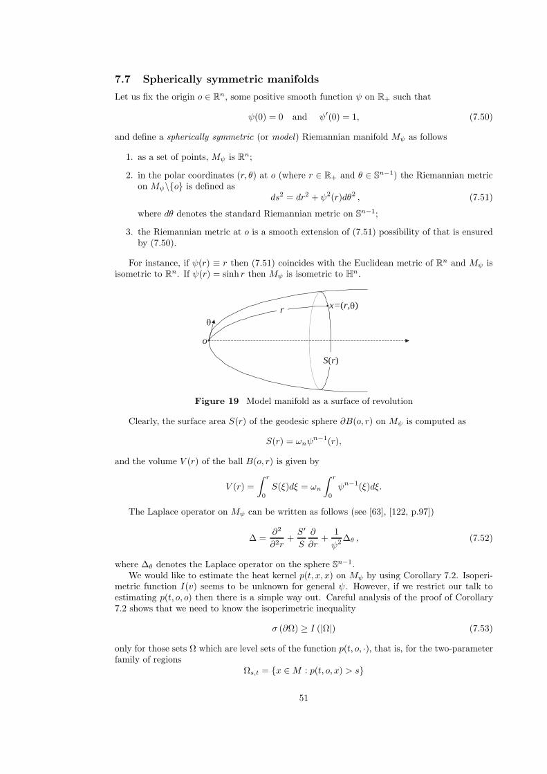
7.7 Spherically symmetric manifolds

Let us fix the origin o ∈ Rn, some positive smooth function ψ on R+ such that

ψ(0) = 0 and ψ′(0) = 1, (7.50)

and define a spherically symmetric (or model) Riemannian manifold Mψ as follows

1. as a set of points, Mψ is Rn;

2. in the polar coordinates (r, θ) at o (where r ∈ R+ and θ ∈ Sn−1) the Riemannian metricon Mψ\o is defined as

ds2 = dr2 + ψ2(r)dθ2 , (7.51)

where dθ denotes the standard Riemannian metric on Sn−1;

3. the Riemannian metric at o is a smooth extension of (7.51) possibility of that is ensuredby (7.50).

For instance, if ψ(r) ≡ r then (7.51) coincides with the Euclidean metric of Rn and Mψ isisometric to Rn. If ψ(r) = sinh r then Mψ is isometric to Hn.

o

x=(r, )r

S(r)

Figure 19 Model manifold as a surface of revolution

Clearly, the surface area S(r) of the geodesic sphere ∂B(o, r) on Mψ is computed as

S(r) = ωnψn−1(r),

and the volume V (r) of the ball B(o, r) is given by

V (r) =∫ r

0

S(ξ)dξ = ωn

∫ r

0

ψn−1(ξ)dξ.

The Laplace operator on Mψ can be written as follows (see [63], [122, p.97])

∆ =∂2

∂2r+S′

S

∂

∂r+

1ψ2 ∆θ , (7.52)

where ∆θ denotes the Laplace operator on the sphere Sn−1.We would like to estimate the heat kernel p(t, x, x) on Mψ by using Corollary 7.2. Isoperi-

metric function I(v) seems to be unknown for general ψ. However, if we restrict our talk toestimating p(t, o, o) then there is a simple way out. Careful analysis of the proof of Corollary7.2 shows that we need to know the isoperimetric inequality

σ (∂Ω) ≥ I (|Ω|) (7.53)

only for those sets Ω which are level sets of the function p(t, o, ·), that is, for the two-parameterfamily of regions

Ωs,t = x ∈M : p(t, o, x) > s

51

(see [36, Proposition 8.1]).Given the rotation symmetry of Mψ with respect to the point o, it is easy to prove that

all Ωs,t are ball centered at o. Hence, we need to find the function I such that (7.53) holdsfor all balls Ω = B(o, r). Since there is only one ball B(o, r) with a prescribed volume, theisoperimetric function I can be defined by

I(v) = S(r) if V (r) = v.

In order to apply Corollary 7.2, I(v)/v should be non-increasing which amounts to thenon-increasing of S(r)/V (r). The equation (7.7) for f(t) becomes

t = 4∫ V −1(f(t))

0

V (r)drS(r)

.

Hence, we arrive to the following conclusion.

Theorem 7.14 ([36, Theorem 8.3]) Suppose that, for a model manifold Mψ, the functionS(r)/V (r) is non-increasing. Let us define the function ρ(t) by

t = 4∫ ρ(t)

0

drddr logV (r)

. (7.54)

Then, for all t > 0 and ε ∈ (0, 1),

p(t, o, o) ≤ CεV (ρ(εt))

. (7.55)

For example, if V (r) = CrN then (7.54) gives ρ(t) √t and (7.55) implies

p(t, o, o) ≤ C′

V (√t)

=C′′

tN/2.

Note that, by Theorem 5.12, we have in this case the matching lower bound for p(t, o, o). Moregenerally, if V (r) is doubling (see (5.38)) then one obtains from Theorems 7.14 and 5.12

p(t, o, o) 1V (

√t)

(see [36, Corollary 8.5]).If V (r) = exp (rα), 0 < α ≤ 1, then we obtain ρ(t) t

12−α and

p(t, o, o) ≤ C exp(−ct α

2−α

). (7.56)

Theorem 5.13 yields for this volume growth the matching lower bound - cf. (5.42).It is interesting that, for covering manifold M with the same volume growth function, the

upper bound (7.48) is weaker than (7.56). In some sense, model manifolds possess the smallestheat kernel per volume growth function. This happens because all directions from o to theinfinity are equivalent, which maximizes the capability of the Brownian motion to escape tothe infinity and, thereby, minimizes the heat kernel p(t, o, o). On covering manifolds, theremay exists two non-equivalent ways of escaping (this is the case, for example, if the desktransformation group Γ is polycyclic) one of them being “narrow” in some sense and providingfor a higher probability of return.

7.8 Manifolds of non-negative Ricci curvature

The main result of this section is the following isoperimetric inequality on non-negatively curvedmanifolds.

52

Theorem 7.15 Let M be a geodesically complete non-compact Riemannian manifold of non-negative Ricci curvature. Then, for any ball B(z,R) ⊂ M and any open set Ω ⊂ B(z,R) withsmooth boundary,

σ (∂Ω)|Ω| ≥ c

R

(V (z,R)

|Ω|)1/n

(7.57)

where n = dimM and c = c(n) > 0.

By Proposition 7.1, the isoperimetric inequality (7.57) implies the relative Faber-Krahninequality (6.42) (the latter was proved for manifolds of non-negative Ricci curvature in [67]).Hence, Theorems 6.13 and 5.9 imply the following upper bound of the heat kernel on M

p(t, x, y) ≤ C√V (x,

√t)V (y,

√t)

exp(−d

2(x, y)2Dt

), (7.58)

where D > 2. This estimate was first obtained by Li and Yau [98]. They also proved thematching lower bound

p(t, x, y) ≥ c√V (x,

√t)V (y,

√t)

exp(−d

2(x, y)2Dt

), (7.59)

for D < 2. Some improvements of these estimates can be found in [93]. See [134], [46] for heatkernel estimates on manifolds with RicM ≥ −K, and [81] for similar heat kernel estimates inunbounded regions in Rn with the Neumann boundary condition.

We precede the proof of (7.57) by two properties of non-negatively curved manifolds.

Lemma 7.16 Let M be a geodesically complete non-compact manifold of non-negative Riccicurvature. Then, for all balls intersecting B(x, r) and B(y, r′) with r ≤ r′,

c

(r′

r

)ε≤ V (y, r′)V (x, r)

≤ C

(r′

r

)n, (7.60)

where ε, c, C are positive and depend on n.

Proof. We use Gromov’s volume comparison theorem which says that if RicM ≥ 0 then, forall x ∈M and r′ ≥ r > 0,

V (x, r′)V (x, r)

≤(r′

r

)n(7.61)

(see [27], [23], [22]).Denote δ = d(x, y). Then δ ≤ r′ + r ≤ 2r′, and the right hand inequality in (7.60) follows

by (7.61)V (y, r′)V (x, r)

≤ V (x, r′ + δ)V (x, r)

≤(r′ + δ

r

)n≤

(3r′

r

)n= 3n

(r′

r

)n.

To prove the left hand inequality in (7.60), let us first verify it in the particular case r′ = 3r andy = x. Find a point ξ such that d(x, ξ) = 2r (here we use the completeness and non-compactnessof M). Then B(ξ, r) is contained in B(x, 3r) but does not intersect B(x, r). Hence, we obtain

V (x, 3r) ≥ V (x, r) + V (ξ, r) ≥ V (x, r)(1 + C−1).

x ξ3r

2rr

Figure 20 Ball B(ξ, r) is contained in B(x, 3r) but does not intersect B(x, r)

53

In general, let us find an integer k such that

3k ≤ r′

r< 3k+1.

ThenV (y, r′) ≥ C−1V (x, r′) ≥ C−1V (x, 3kr) ≥ C−1(1 + C−1)kV (x, r)

andV (y, r′)V (x, r)

≥ C−1(1 + C−1

)k ≥ c

(r′

r

)log3(1+C−1),

which was to be proved.

Lemma 7.17 (Buser [18]) Let M be a geodesically complete manifold of non-negative Riccicurvature. Then, for any ball B(x, r) and for any smooth hypersurface Γ in B(x, r) dividingB(x, r) into two sets both having volume at least v,

σ (Γ) ≥ cv

r, (7.62)

where c = c(n) > 0.

Observe that inequality (7.62) follows from (7.32) if M = Rn. We refer the reader to [18,Lemma 5.1] or [67, Theorem 2.1] for the proof in general case.Proof of Theorem 7.15. The proof is similar to Theorem 7.7. For any point x ∈ Ω, let usfind a positive r(x) so that Ω covers exactly one half of the volume of B(x, r(x)). To that end,consider the function

h(r) :=|Ω ∩B(x, r)|V (x, r)

.

For r small enough, we have h(r) = 1. If r > R then, by Lemma 7.16,

h(r) ≤ |Ω|V (x, r)

≤ V (z,R)V (x, r)

≤ c−1

(R

r

)ε.

In particular, if the ratio r/R is large enough then h(r) < 1/2. Hence, for some r ≤ C′R, wehave h(r) = 1/2.

The family of balls B(x, r(x)), x ∈ Ω, covers Ω. By using the Banach ball covering argument,we can select at most countable subset B(xi, ri) (where ri = r(xi)) so that the balls B(xi, ri)are disjoint whereas the union of B(xi, 5ri) covers Ω. The latter implies∑

i

V (xi, ri) ≥ 5−n∑i

V (xi, 5ri) ≥ 5−n |Ω| . (7.63)

On the other hand, Lemma 7.17 and the fact that

|Ω ∩B(xi, ri)| =12V (xi, ri),

implyσ (∂Ω ∩B(xi, ri)) ≥ c

2riV (xi, ri). (7.64)

Ω

B(xi, ri)

= B(xi,ri)

Figure 21 Estimating the area of Γ via the volumes of the sets Ω∩B(xi, ri) and B(xi, ri) \Ω

54

SinceV (z,R)V (x, ri)

≤ V (x,R + ri)V (x, ri)

≤ V (x,R(1 + C′))V (x, ri)

≤ C′′(R

ri

)n,

we have1ri

≥ c′

R

(V (z,R)V (x, ri)

)1/n

.

By substituting into (7.64), we obtain

σ (∂Ω ∩B(xi, ri)) ≥ c′

RV (z,R)1/nV (xi, ri)1−1/n.

Finally, summing up over all i and applying (7.33) and (7.63), we conclude

σ (∂Ω) ≥ c′′

RV (z,R)1/n |Ω|1−1/n

,

which is equivalent to (7.57).By Corollary 6.14, the upper bound (7.58) is equivalent to the relative Faber-Krahn in-

equality, under the standing assumption of the doubling volume property. It turns out thatthe conjunction of both upper and lower bounds (7.58) and (7.59) is equivalent to the Poincareinequality ∫

B(x,2r)

|∇f |2 dµ ≥ c

r2infξ∈R

∫B(x,r)

(f − ξ)2 dµ , (7.65)

which is meant to hold for all x ∈ M , r > 0 and f ∈ C1(B(x, 2r)) (see [67], [68], [120], [121]).One can regard (7.65) as the L2-version of the isoperimetric inequality (7.62). Indeed, the lateris equivalent to the functional inequality∫

B(x,2r)

|∇f |dµ ≥ c

r2infξ∈R

∫B(x,r)

|f − ξ| dµ. (7.66)

Theorem 7.15 can be stated as the implication (7.66)⇒(7.57). Similarly, one can prove that(7.65) implies the relative Faber-Krahn inequality (6.42) - see [67, Theorem 1.4] and [120,Theorem 2.1].

References

[1] Alexopoulos G.K., A lower estimate for central probabilities on polycyclic groups, Can.J. Math., 44 (1992) no.5, 897-910.

[2] Alexopoulos G.K., An application of Homogenization theory to Harmonic analysis onsolvable Lie groups of polynomial growth, Pacific J. Math., 159 (1993) 19-45.

[3] Anker J-Ph., Ji L., Heat kernel and Green function estimates on non-compact symmetricspaces, preprint

[4] Aronson D.G., Bounds for the fundamental solution of a parabolic equation, Bull. ofAMS, 73 (1967) 890-896.

[5] Azencott R., Behavior of diffusion semi-groups at infinity, Bull. Soc. Math. (France),102 (1974) 193-240.

[6] Barbatis G., Davies E.B., Sharp bounds on heat kernels of higher order uniformlyelliptic operators, J. Operator Theory, 36 (1996) 179–198.

[7] Barlow M., Diffusion on fractals, Lecture notes

55

[8] Barlow M., Bass R., Transition densities for Brownian motion on the Sierpinski carpet,Probab. Th. Rel. Fields, 91 (1992) 307–330.

[9] Barlow M., Bass R., Brownian motion and harmonic analysis on Sierpinski carpets, toappear in Canad. J. Math.

[10] Barlow M., Perkins A., Brownian motion on the Sierpinski gasket, Probab. Th. Rel.Fields, 79 (1988) 543–623.

[11] Batty C.J.K., Bratelli O., Jorgensen P.E.T., Robinson D.W., Asymptotics ofperiodic subelliptic operators, preprint

[12] Ben Arous G., Leandre R., Decroissance exponentielle du noyau de la chaleur sur ladiagonale 1,2, Prob. Th. Rel. Fields, 90 (1991) 175-202 and 377-402.

[13] Bendikov A., “Potential theory on infinite dimensional Ablelian groups” De Gruyter,1995.

[14] Bendikov A., Saloff-Coste L., Elliptic operators on infinite products, J. Reine Angew.Math., 493 (1997) 171–220.

[15] Benjamini I., Chavel I., Feldman E.A., Heat kernel lower bounds on Riemannianmanifolds using the old ideas of Nash, Proceedings of London Math. Soc., 72 (1996)215-240.

[16] Bombieri E., de Giorgi E., Miranda M., Una maggiorazioni a-priori relative alleipersuperfici minimali non parametriche, Arch. Rat. Mech. Anal., 32 (1969) 255-367.

[17] Brooks R., A relation between growth and the spectrum of the Laplacian, Math. Z.,178 (1981) 501-508.

[18] Buser P., A note on the isoperimetric constant, Ann. Scient. Ec. Norm. Sup., 15 (1982)213-230.

[19] Carlen E.A., Kusuoka S., Stroock D.W., Upper bounds for symmetric Markovtransition functions, Ann. Inst. H. Poincare, Prob. et Stat., (1987) suppl. au no.2,245-287.

[20] Carron G., Inegalites isoperimetriques de Faber-Krahn et consequences, in: “Actes dela table ronde de geometrie differentielle en l’honneur de Marcel Berger”, Collection SMFSeminaires et Congres, no.1, 1994.

[21] Carron G., Inegalites de Sobolev-Orlicz non-uniformes, preprint 1996.

[22] Chavel I., “Eigenvalues in Riemannian geometry” Academic Press, New York, 1984.

[23] Chavel I., “Riemannian geometry : a modern introduction” Cambridge Tracts in Math-ematics 108, Cambridge University Press, 1993.

[24] Chavel I., “Large time heat diffusion on Riemannian manifolds” Lecture notes 1998.

[25] Chavel I., Feldman E.A., Modified isoperimetric constants, and large time heat diffu-sion in Riemannian manifolds, Duke Math. J., 64 (1991) no.3, 473-499.

[26] Cheeger J., A lower bound for the smallest eigenvalue of the Laplacian, in: “Problemsin Analysis: A Symposium in honor of Salomon Bochner”, Princeton University Press.Princeton, 1970. 195-199.

[27] Cheeger J., Gromov M., Taylor M., Finite propagation speed, kernel estimates forfunctions of the Laplace operator, and the geometry of complete Riemannian manifolds, J.Diff. Geom., 17 (1982) 15-53.

56

[28] Cheeger J., Yau S.-T., A lower bound for the heat kernel, Comm. Pure Appl. Math.,34 (1981) 465-480.

[29] Cheng S.Y., Li P., Yau S.-T., On the upper estimate of the heat kernel of a completeRiemannian manifold, Amer. J. Math., 103 (1981) no.5, 1021-1063.

[30] Chung F.R.K., “Spectral Graph Theory” AMS publications, 1996.

[31] Chung F.R.K., Grigor’yan A., Yau S.-T., Upper bounds for eigenvalues of thediscrete and continuous Laplace operators, Advances in Math., 117 (1996) 165-178.

[32] Chung F.R.K., Grigor’yan A., Yau S.-T., Eigenvalues and diameters for manifoldsand graphs, in: “Tsing Hua Lectures on Geometry and Analysis”, ed. S.-T.Yau, Interna-tional Press, 1997. 79-105.

[33] Chung F.R.K., Grigor’yan A., Yau S.-T., Higher eigenvalues and isoperimetricinequalities on Riemannian manifolds and graphs, to appear in Comm. Anal. Geom

[34] Coulhon T., Noyau de la chaleur et discretisation d’une variete riemannienne, Israel J.Math., 80 (1992) 289-300.

[35] Coulhon T., Ultracontractivity and Nash type inequalities, J. Funct. Anal., 141 (1996)510-539.

[36] Coulhon T., Grigor’yan A., On-diagonal lower bounds for heat kernels on non-compactmanifolds and Markov chains, Duke Math. J., 89 (1997) no.1, 133-199.

[37] Coulhon T., Grigor’yan A., Random walks on graphs with regular volume growth,Geom. and Funct. Analysis, 8 (1998) 656-701.

[38] Coulhon T., Saloff-Coste L., Isoperimetrie pour les groupes et les varietes, RevistaMathematica Iberoamericana, 9 (1993) no.2, 293-314.

[39] Coulhon T., Saloff-Coste L., Minorations pour les chaınes de Markov unidimension-nelles, Prob. Theory Relat. Fields, 97 (1993) 423-431.

[40] Davies B., Simon B., Ultracontractivity and the heat kernel for Schrodinger operatorsand Dirichlet Laplacians, J. Funct. Anal., 59 (1984) 335-395.

[41] Davies E.B., Explicit constants for Gaussian upper bounds on heat kernels, Amer. J.Math., 109 (1987) 319-334.

[42] Davies E.B., Gaussian upper bounds for the heat kernel of some second-order operatorson Riemannian manifolds, J. Funct. Anal., 80 (1988) 16-32.

[43] Davies E.B., “Heat kernels and spectral theory” Cambridge University Press, Cam-bridge, 1989.

[44] Davies E.B., Pointwise bounds on the space and time derivatives of the heat kernel, J.Operator Theory, 21 (1989) 367-378.

[45] Davies E.B., Heat kernel bounds, conservation of probability and the Feller property,J. d’Analyse Math., 58 (1992) 99-119.

[46] Davies E.B., The state of art for heat kernel bounds on negatively curved manifolds,Bull. London Math. Soc., 25 (1993) 289-292.

[47] Davies E.B., Uniformly elliptic operators with measurable coefficients, J. Func. Anal.,132 (1995) 141-169.

[48] Davies E.B., Lp spectral theory of higher-order elliptic differential operators, Bull.London Math. Soc., 29 (1997) 513-546.

57

[49] Davies E.B., Non-Gaussian aspects of heat kernel behaviour, J. London Math. Soc., 55(1997) no.1, 105-125.

[50] Davies E.B., Mandouvalos N., Heat kernel bounds on hyperbolic space and Kleiniangroups, Proc. London Math. Soc.(3), 52 (1988) no.1, 182-208.

[51] Davies E.B., Pang M.M.H., Sharp heat kernel bounds for some Laplace operators,Quart. J. Math., 40 (1989) 281-290.

[52] Debiard A., Gaveau B., Mazet E., Theoremes de comparison in geometrie riemanni-enne, Publ. Kyoto Univ., 12 (1976) 391-425.

[53] Delmotte T., Parabolic Harnack inequality and estimates of Markov chains on graphs,preprint

[54] DiBenedetto E., “Degenerate parabolic equations” Universitext, Springer,

[55] Dodziuk J., Maximum principle for parabolic inequalities and the heat flow on openmanifolds, Indiana Univ. Math. J., 32 (1983) no.5, 703-716.

[56] Dodziuk J., Mathai V., Approximating L2 invariants of amenable covering spaces: aheat kernel approach, preprint

[57] Donnelly H., Heat equation asymptotics with torsion, Indiana Univ. Math. J., 34(1985) no.1, 105–113.

[58] Donnelly H., Essential spectrum and heat kernel, J. Funct. Anal., 75 (1987) no.2,362–381.

[59] Erdos L., Estimates on stochastic oscillatory integrals and on the heat kernel of themagnetic Schrodinger operator, Duke Math. J., 76 (1994) 541-566.

[60] Fabes E.B., Stroock D.W., A new proof of Moser’s parabolic Harnack inequality viathe old ideas of Nash, Arch. Rat. Mech. Anal., 96 (1986) 327-338.

[61] Federer H., Fleming W.H., Normal and integral currents, Ann. Math., 72 (1960)458-520.

[62] Gilkey P.B., “The index theorem and the heat equation” Publish or Perish, BostonMA, 1974.

[63] Greene R., Wu W., “Function theory of manifolds which possess a pole” Lecture Notesin Math. 699, Springer, 1979.

[64] Grigor’yan A., Isoperimetric inequalities for Riemannian products, (in Russian) Mat.Zametki, 38 (1985) no.4, 617-626. Engl. transl. Math. Notes, 38 (1985) 849-854.

[65] Grigor’yan A., On stochastically complete manifolds, (in Russian) DAN SSSR, 290(1986) no.3, 534-537. Engl. transl. Soviet Math. Dokl., 34 (1987) no.2, 310-313.

[66] Grigor’yan A., On the fundamental solution of the heat equation on an arbitrary Rie-mannian manifol, (in Russian) Mat. Zametki, 41 (1987) no.3, 687-692. Engl. transl. Math.Notes, 41 (1987) no.5-6, 386-389.

[67] Grigor’yan A., The heat equation on non-compact Riemannian manifolds, (in Russian)Matem. Sbornik, 182 (1991) no.1, 55-87. Engl. transl. Math. USSR Sb., 72 (1992) no.1,47-77.

[68] Grigor’yan A., Heat kernel on a non-compact Riemannian manifold, in: “1993 SummerResearch Institute on Stochastic Analysis”, ed. M.Pinsky et al., Proceedings of Symposiain Pure Mathematics, 57 (1994) 239-263.

58

[69] Grigor’yan A., Heat kernel upper bounds on a complete non-compact manifold, RevistaMathematica Iberoamericana, 10 (1994) no.2, 395-452.

[70] Grigor’yan A., Heat kernel on a manifold with a local Harnack inequality, Comm. Anal.Geom., 2 (1994) no.1, 111-138.

[71] Grigor’yan A., Upper bounds of derivatives of the heat kernel on an arbitrary completemanifold, J. Funct. Anal., 127 (1995) no.2, 363-389.

[72] Grigor’yan A., Gaussian upper bounds for the heat kernel on arbitrary manifolds, J.Diff. Geom., 45 (1997) 33-52.

[73] Grigor’yan A., Escape rate of Brownian motion on weighted manifolds, to appear inApplicable Analysis

[74] Grigor’yan A., Analytic and geometric background of recurrence and non-explosionof the Brownian motion on Riemannian manifolds, Bull. Amer. Math. Soc., 36 (1999)135-249.

[75] Grigor’yan A., Kelbert M., Range of fluctuation of Brownian motion on a completeRiemannian manifold, Ann. Prob., 26 (1998) 78-111.

[76] Grigor’yan A., Kelbert M., On Hardy-Littlewood inequality for Brownian motion onRiemannian manifolds, to appear in J. London Math. Soc.

[77] Grigor’yan A., Noguchi M., The heat kernel on hyperbolic space, Bull. London Math.Soc., 30 (1998) 643-650.

[78] Grigor’yan A., Saloff-Coste L., Heat kernel on connected sums of Riemannian mani-folds, to appear in Math. Research Letters

[79] Guivarc’h Y., Sur la loi des grands nombres et le rayon spectral d’une marche aleatoire,Journee sur les marches aleatoires, Asterisque, 74 (1980) 47-98.

[80] Gushchin A.K., On the uniform stabilization of solutions of the second mixed problemfor a parabolic equation, (in Russian) Matem. Sbornik, 119(161) (1982) no.4, 451-508.Engl. transl. Math. USSR Sb., 47 (1984) 439-498.

[81] Gushchin A.K., Michailov V.P., Michailov Ju.A., On uniform stabilization of thesolution of the second mixed problem for a second order parabolic equation, (in Russian)Matem. Sbornik, 128(170) (1985) no.2, 147-168. Engl. transl. Math. USSR Sb., 56 (1987)141-162.

[82] Hamilton R.S., A matrix Harnack estimate for the heat equation, Comm. Anal. Geom.,1 (1983) no.1, 113–126.

[83] Hebisch W., Saloff-Coste, L., Gaussian estimates for Markov chains and random walkson groups, Ann. Prob., 21 (1993) 673–709.

[84] Hoffman D., Spruck J., Sobolev and isoperimetric inequalities for Riemannian subman-ifolds, Comm. Pure Appl. Math., 27 (1974) 715–727. See also “A correction to: Sobolevand isoperimetric inequalities for Riemannian submanifolds”, Comm. Pure Appl. Math.,28 (1975) no.6, 765–766.

[85] Hsu E.P., Short-time asymptotics of the heat kernel on a concave boundary, SIAM J.Math. Anal., 20 (1989) no.5, 1109-1127.

[86] Hsu E.P., Estimates of derivatives of the heat kernel on a compact Riemannian manifolds,preprint

59

[87] Kanai M., Rough isometries, and combinatorial approximations of geometries of non-compact Riemannian manifolds, J. Math. Soc. Japan, 37 (1985) 391-413.

[88] Kanai M., Rough isometries and the parabolicity of manifolds, J. Math. Soc. Japan, 38(1986) 227-238.

[89] Kotani M., Shirai T., Sunada T., Asymptotic behavior of the transition probabilityof a random walk on an infinite graph, J. Func. Anal., 159 (1998) 664-689.

[90] Kotani M., Sunada T., Albanese maps and off diagonal long time asymptotics for theheat kernel, preprint

[91] Kusuoka S., Stroock D.W., Long time estimates for the heat kernel associated withuniformly subelliptic symmetric second order operators, Ann. Math., 127 (1989) 165-189.

[92] Leandre R., Uniform upper bounds for hypoelliptic kernels with drift, J. Math. KyotoUniv., 34 no.2, (1994) 263-271.

[93] Li P., Large time behavior of the heat equation on complete manifolds with nonnegativeRicci curvature, Ann. Math., 124 (1986) 1–21.

[94] Li P., Harmonic sections of polynomial growth, Math. Research Letters, 4 (1997) no.1,35–44.

[95] Li P., Schoen R., Lp and mean value properties of subharmonic functions on Riemannianmanifolds, Acta Math., 153 (1984) 279-301.

[96] Li P., Wang J., Convex hull properties of harmonic maps, J. Diff. Geom., 48 (1998)497-530.

[97] Li P., Wang J., Mean value inequalities, preprint

[98] Li P., Yau S.-T., On the parabolic kernel of the Schrodinger operator, Acta Math., 156(1986) no.3-4, 153-201.

[99] Liskevich V., Semenov Yu., Two-sided estimates of the heat kernel of the Schrodingeroperator, Bull. London Math. Soc., 30 (1998) 596-602.

[100] Malliavin P., Stroock D.W., Short time behavior of the heat kernel and its logarithmicderivatives, J. Diff. Geom., 44 (1996) 550-570.

[101] Maz’ya V.G., Classes of domains and embedding theorems for functional spaces, (inRussian) Dokl. Acad. Nauk SSSR, 133 no.3, (1960) 527-530. Engl. transl. Soviet Math.Dokl., 1 (1961) 882-885.

[102] Maz’ya V.G., “Sobolev spaces” (in Russian) Izdat. Leningrad Gos. Univ. Leningrad,1985. Engl. transl. Springer, 1985.

[103] McKean H.P., An upper bound to the spectrum of ∆ on a manifold of negativecurvature, J. Diff. Geom., 4 (1970) 359–366.

[104] Michael J.H., Simon L.M., Sobolev and mean-value inequalities on generalized sub-manifolds of Rn, Comm. Pure Appl. Math., 26 (1973) 361-379.

[105] Molchanov S.A., Diffusion processes and Riemannian geometry, (in Russian) UspekhiMatem. Nauk, 30 (1975) no.1, 3-59. Engl. transl. Russian Math. Surveys, 30 (1975) no.1,1-63.

[106] Moser J., A Harnack inequality for parabolic differential equations, Comm. Pure Appl.Math., 17 (1964) 101-134.

60

[107] Murata M., Large time asymptotics for fundamental solutions of diffusion equations,Tohoku Math. J., 37 (1985) 151-195.

[108] Mustapha S., Gaussian estimates for heat kernels on Lie groups, preprint

[109] Nash J., Continuity of solutions of parabolic and elliptic equations, Amer. J. Math.,80 (1958) 931-954.

[110] Norris J.R., Heat kernel bounds and homogenization of elliptic operators, Bull. LondonMath. Soc., 26 (1994) 75-87.

[111] Norris J.R., Long time behaviour of heat flow: global estimates and exact asymptotics,preprint

[112] Norris J.R., Heat kernel asymptotics and the distance function for measurable Rie-mannian metrics, preprint

[113] Osserman R., Minimal varieties, Bull. Amer. Math. Soc., 75 (1969) 1092-1120.

[114] Pittet Ch., Saloff-Coste L., A survey on the relationship between volume growth,isoperimetry, and the behavior of simple random walk on Cayley graphs, with examples,preprint

[115] Pittet Ch., Saloff-Coste L., Amenable groups, isoperimetric profiles and randomwalks, in: “Geometric group theory down under. Proceedings of a special year in geometricgroup theory, Canberra, Australia, 1996”, ed. J. Cossey, C.F. Miller III, W.D. Neumannand M. Shapiro, Walter De Gruyter, 1999.

[116] Porper F.O., Eidel’man S.D., Two-side estimates of fundamental solutions of second-order parabolic equations and some applications, (in Russian) Uspekhi Matem. Nauk, 39(1984) no.3, 101-156. Engl. transl. Russian Math. Surveys, 39 (1984) no.3, 119-178.

[117] Qian Z., Gradient estimates and heat kernel estimates, Proc. Roy. Soc. Edinburgh,125A (1995) 975-990.

[118] Robinson D.W., “Elliptic operators and Lie groups” Oxford Math. Mono., ClarentonPress, Oxford New York Tokyo, 1991.

[119] Rosenberg S., “The Laplacian on a Riemannian manifold” Student Texts 31, LondonMathematical Society, 1991.

[120] Saloff-Coste L., A note on Poincare, Sobolev, and Harnack inequalities, Duke MathJ., I.M.R.N., 2 (1992) 27-38.

[121] Saloff-Coste L., Parabolic Harnack inequality for divergence form second order differ-ential operators, Potential Analysis, 4 (1995) 429-467.

[122] Schoen R., Yau S.-T., “Lectures on Differential Geometry” Conference Proceedingsand Lecture Notes in Geometry and Topology 1, International Press, 1994.

[123] Semenov Yu.A., On perturbation theory for linear elliptic and parabolic operators; themethod of Nash, Contemporary Math., 221 (1999) 217-284.

[124] Stroock D.W., Estimates on the heat kernel for the second order divergence form op-erators, in: “Probability theory. Proceedings of the 1989 Singapore Probability Conferenceheld at the National University of Singapore, June 8-16 1989”, ed. L.H.Y. Chen, K.P. Choi,K. Hu and J.H. Lou, Walter De Gruyter, 1992. 29-44.

[125] Stroock D.W., Turetsky J., Upper bounds on derivatives of the logarithm of the heatkernel, preprint

61

[126] Sturm K-Th., Heat kernel bounds on manifolds, Math. Ann., 292 (1992) 149-162.

[127] Sturm K-Th., Analysis on local Dirichlet spaces II. Upper Gaussian estimates for thefundamental-solutions of parabolic equations, Osaka J. Math, 32 (1995) no.2, 275-312.

[128] Sturm K-Th., Analysis on local Dirichlet spaces III. The parabolic Harnack inequality,Journal de Mathematiques Pures et Appliquees, 75 (1996) no.3, 273-297.

[129] Ushakov V.I., Stabilization of solutions of the third mixed problem for a second orderparabolic equation in a non-cylindric domain, (in Russian) Matem. Sbornik, 111 (1980)95-115. Engl. transl. Math. USSR Sb., 39 (1981) 87-105.

[130] Varadhan S.R.S., On the behavior of the fundamental solution of the heat equationwith variable coefficients, Comm. Pure Appl. Math., 20 (1967) 431-455.

[131] Varadhan S.R.S., Diffusion processes in a small time interval, Comm. Pure Appl.Math., 20 (1967) 659-685.

[132] Varopoulos N.Th., Brownian motion and random walks on manifolds, Ann. Inst.Fourier, 34 (1984) 243-269.

[133] Varopoulos N.Th., Hardy-Littlewood theory for semigroups, J. Funct. Anal., 63(1985) no.2, 240-260.

[134] Varopoulos N.Th., Small time Gaussian estimates of heat diffusion kernel. I. Thesemigroup technique, Bull. Sci. Math.(2), 113 (1989) no.3, 253-277.

[135] Varopoulos N.Th., Saloff-Coste L., Coulhon T., “Analysis and geometry ongroups” Cambridge University Press, Cambridge, 1992.

[136] Woess W., “Random walks on infinite graphs and groups”

[137] Yafaev D., Spectral properties of the Schrodinger operator with positive slowly decreas-ing potential, (in Russian) Funktsional. Anal. i Prilozhen., 16 (1982) 47–54. Engl. transl.Functional Anal. Appl., 16 (1982) no.4, 280–285.

[138] Yau S.-T., Harmonic functions on complete Riemannian manifolds, Comm. Pure Appl.Math., 28 (1975) 201-228.

[139] Yau S.-T., Isoperimetric constant and the first eigenvalue of a compact Riemannianmanifold, Ann. Sci. Ecole Norm. Sup., 4th serie, 8 no.4, (1975) 487-507.

[140] Yau S.-T., On the heat kernel of a complete Riemannian manifold, J. Math. PuresAppl., ser. 9, 57 (1978) 191-201.

[141] Yau S.-T., Harnack inequality for non-self-adjoint evolution equations, Math. ResearchLetters, 2 (1995) 387-399.

62