Estimates of Oil ReservesJean Laherrere

e-mail: jean.laherrere@wanadoo.frsites: http://www.oilcrisis.com/laherrere/

http://mwhodges.home.att.net/energy/energy.htmJune 10, 2001

Paper presented at the EMF/IEA/IEW meetingIIASA, Laxenburg, Austria - June 19, 2001

Plenary Session I: Resources

This document for the IIASA site gathers many graphs and a long text for those who want to gettechnical data on many countries and explanations, but only a part will be shown during mypresentation.

My apologies for my broken English

1 What oil? ......................................................................................................................................32 Reports: what is published could be different from technical results! .........................................93 Assessments................................................................................................................................134 Examples of reserve & production data from countries.............................................................255 Reserve growth...........................................................................................................................476 Reserves & Resources ................................................................................................................607 Ultimates ....................................................................................................................................628 Forecasts.....................................................................................................................................709 Future production .......................................................................................................................7410 Impact on climate change: IPCC scenarios............................................................................83Conclusions: .......................................................................................................................................90References: .........................................................................................................................................91

2

Introduction

The western world lives in a culture of belief in growth and everyone hopes to see their childrenhaving better lives than they had, but for the first time we are not sure. Everyone would like to seethe growth continue and hates to speak about decline.

Politicians promise that growth will solve the present problems on welfare, retirement and theywould dearly love to see the reserves of oil, which fuels the economy, grow.

As the French writer Antoine de Saint Exupery wrote: “we do no inherit from our parents, weborrow from our children”

There are two schools on reserves but also much the confusion between reserves and resources.

The views of so-called “Pessimists” (mainly retired geologists or retired CEO (Bernabe 1998,Bowlin 1999) are compared with those of so-called ”Optimists” (mainly economists Aldeman,Lynch, or governmental agencies DOE, IEA, EU)

The Pessimists have access to technical data when the Optimists have access to political or financialdata.

Reporting data on oil production or oil reserves is a political act. The SEC, to satisfy bankers andshareholders, obliges the oil companies listed on the US stock market to report only ProvedReserves and to omit Probable Reserves that are reported in the rest of the world. This poor practiceof reporting only Proved Reserves led to a strong reserve growth, as 90% of the annual reserves oiladdition come from revisions of old fields, showing that the assessment of the fields was poorlyreported. This reserve growth of conventional oil reserves is wrongly attributed to technologicalprogress. Technical data, on which development decisions are taken, exist but they are confidential.There are database companies (or “scout” data as a scout is someone sent to get information withoutrevealing his source), selling technical data, but these databases are very expensive.

Reporting of reserves is poor, but reporting on production is not much better as the 10$/b of early1999 seems to be mainly due to the « missing barrels » of IEA overestimating the supply andunderestimating the demand (end of Asiatic crisis), giving a false impression of oil abundance(Simmons 2000).

Recovery factor is assumed to depend mainly upon oil price, when it depends mainly on thegeology and physics of the reservoir.

The Optimists believe that technology (as Santa Claus) will solve all the problems, but they do notwant to listen to technicians who say that technology has limits.

The Greek philosopher Esopus said that the tongue was the best tool (when saying words of love orpoetry) and the worst tool (when shouting hate or murder).

The oil industry uses also the best and the worst technology. The best technology is in seismic,logging, producing. The worst technology is in defining units, measuring, reporting andcommunicating about oil. The oil industry is not alone. The $125 million Mars spacecraft was lostbecause NASA navigators mistakenly thought a contractor used metric measurements. Thecontractor had used English units, and the probe burned up in the Martian atmosphere on Sept. 23,1999. The computer industry was not very bright in letting the Y2K bug to occur, but the worst wasthat there was no bug at all, even for the countries, which did not bother to correct it. The last USpresidential elections with obsolete punched cards and poor machines are a bad image of moderntechnology. The blackouts of California confirm this poor image.

3

The importance of oil was recently denied in front of the emergence of Internet or the huge increaseof GPD (manipulated to show growth). But the new economy has been badly damaged by the lastoil shock.

Published data are unreliable and the image of the oil industry given by different actors confusing.As an uncertain estimate has to be given within a range and not by one single number, the ways ofdescribing the oil industry would show their strengths and also their weaknesses. I claim to be a oilexplorer as a geologist-geophysicist who has participated in finding many oil fields including somegiants ones (the first one being Hassi Messaoud (Algeria 10 Gb) and the last one Cusiana(Colombia 0.7 Gb), but I drilled a lot of dry holes. It is only by recognising the errors that progresscan be made (the “trial and error” approach in mathematics when a solution is not available).Claiming that an author is wrong because he was wrong once is denying progress. Only perseveringin obsolete practice should be reprimanded.

1 What oil?

There is a lack of definitions and consensus as everyone wants to be free to say what he wants.People are very conservative and reluctant to change, keeping obsolete units and terms.

1.1 What product?

Oil could be crude oil (2000 World 65 Mb/d, but 68 Mb/d with lease condensate) or petroleum (76Mb/d), which includes the condensate (from separator on wellhead), natural gas liquids (NGL fromgas processing plants), synthetic oil, refinery processing gains, other oils and stock withdrawal.

NGL could include or not the condensate, in the US lease condensate is included with the oil, but inOPEC the oil quotas exclude condensate.

The world’s oil supply is given for 1998 to 2000 as in Mb/d:

WO CGES DOE oil+NGL BP DOE oil OGJ OPEC

1998 75.4 75.3 73.6 73.4 67 66.2 65.5

1999 74.1 74 71.9 65.7 64.7 64

2000 76.7 76.7 68.2 67.1

Sources: World Oil, Oil & Gas Journal, BP Review, USDOE/EIA, OPEC Bulletin, Centre for Global Energy Studies

In addition to the petroleum gathered from production plants as crude oil, condensate, natural gasliquids, synthetic oil, there are also the liquids from the refinery reported as of the processing gains,being about 1.7 Mb/d/ But the supply is also different from the demand as there is petroleumcoming from stocks withdrawal which varies about plus or minus 1.5 Mb/d.

CGES 1998 1999 2000

Processing gains 1.6 1.7 1.7

Supply less demand 1.5 -1.2 0.4

This explains the discrepancy of about 3 Mb/d which can be found in the values of the petroleumproduction from different sources, in addition of the 6 Mb/d coming from gas liquids.

For 1998 the US production of NGL is reported in EIA ar98 as 833 Mb and in EIA aer99 (NaturalGas Plant Liquids Production) as 642 Mb, which is a difference of 30%

4

In the US, the importance of the NGL (24%) and the processing gain (12%) versus the domesticproduction has to be noted.

US supply for 1999 Mb/d % % domestic

crude & condensate 5.88 30 76

NGL 1.85 9 24

total liquids production 7.73 40 100

imports 9.91 51 128

processing gain 0.89 5 12

withdrawal 0.3 2 4

alcohol 0.38 2 5

others 0.31 2 4

total supply 19.52 100 253

Oil and gas could be conventional or unconventional (or non-conventional).

Conventional covers usually primary and secondary recovery for porous and permeable reservoir,identified water contact and oil characteristic (light and medium gravity and not viscous oil).

Unconventional covers unusual reservoir characteristics, enhanced oil recovery (tertiary recovery),extra heavy oils (heavier than water), tarsands (defined by viscosity over 10 000 cP), tight reservoir,coalbed methane, geopressured aquifers, methane hydrates, oil shales (in fact mainly immaturesource-rock which should be classified as coal). Some include deepwater (vary from author from200 m to 1000 m), ultradeepwater (over 2000 m), Arctic.

USGS define unconventional as continuous type accumulations where there is no defined watercontact.

Oil supply differs from demand by the change in stocks

EIA STEO Aug 2000 1999 2000

Demand world Mb/d 74.8 75.8

Supply world Mb/d 73.9 76.6

The inventory of supply and demand is neither easy to come by nor reliable. The InternationalEnergy Agency (IEA) in Paris is generally regarded as the best source, but many errors haveoccurred. The exceptional low price of 10$/b in 1998 was due to the mistaken decision to increaseOPEC quotas in the face of the Asian recession and a serious over-estimation of the supply (300 to600 Mb) by the IEA (the “missing barrels”: Simmons 2000).

1.2 Measures?

1.2.1 Volume or weight or energy

Oil could be measured as volume (measurements of flow in a pipe or in a container) or as weight. Infact if one is chosen, the density has to be given too (it varies with time), as it is impossible toconvert one into the other with accuracy without knowing its density. To compare energy, oilequivalence is often used but also the energy (or calorific or work) unit in Btu (British thermal unit)or Joule (work, energy and heat unit). Btu is very small unit (the heat in a wooden head match) andJoule is about one thousand times larger and corresponds to the work of moving one water litre by10 cm, 1 Btu = 1005.06 J. Btu is banished from the EU since the end of 1979.

5

Oil could be given either in gallons, barrel, cubic meter, ton, exajoule (EJ= 10E18 J), Btu (quad=quadrillion Btu ≈ EJ)

In UK and France, oil and condensate (in fact NGL) are given in ton, but in Norway oil, andcondensate are in cubic meter (as Canada) but NGL in ton, in US oil and condensate in barrel(condensate could be in barrel oil equivalent different from the measured volume). WEA in gigatonand exajoule, IEA& WEC in gigaton.

The oil density varies between 740 and 1030 kg/m3 (60°API to 6°API) and could beexpressed in barrel per ton. But what is published is often contradictory.

OPEC statistics - Conversion factors for Crude oil in barrel per ton

By country 1995 1996 1997 1998 1999

Algeria 7.7741 7.7741 7.7741 7.9448 7.9448

Indonesia 7.7600 7.7600 7.7600 7.2338 7.2338

IR Iran 7.3145 7.3145 7.3145 7.2957 7.2840

Iraq 7.4530 7.4530 7.4530 7.4127 7.4127

Kuwait 7.2622 7.2460 7.2460 7.246 7.2580

SP Libyan AJ 7.5876 7.5876 7.5876 7.5584 7.5584

Nigeria 7.3540 7.3540 7.3540 7.4114 7.4114

Qatar 7.6058 7.6058 7.6058 7.5898 7.6180

Saudi Arabia 7.3229 7.3229 7.3229 7.2843 7.2845

United Arab Emirates 7.5964 7.5964 7.5964 7.5875 7.5532

Venezuela 6.9337 6.9488 6.9580 7.3104 7.1210

Average OPEC 7.3661 7.3671 7.3718 7.3677 7.3464

It shows a false or virtual accuracy and political change (no change and sudden jumps)

But BP Review gives both barrels and tons, and the corresponding density is different, as forexample Saudi Arabia is not 7.3 b/t but 7.6 b/t, Algeria is not 7.9 but 8.7.

BP Statistical Review 2000Oil: Production 1999 Mt Mb b/tUSA 354.7 2832 8Canada 120.3 947 7.9Mexico 166.1 1221 7.4Total North America 641.1 5001 7.8Argentina 42.7 310 7.3Brazil 56.3 407 7.2Colombia 42.5 307 7.2Ecuador 19.5 139 7.1Peru 5.5 40 7.3Trinidad & Tobago 6.6 49 7.5Venezuela 160.5 1141 7.1Other S. & C. America 6.6 49 7.5Total S. & C. America 340.2 2442 7.2Denmark 14.5 110 7.6Italy 5.6 40 7.2Norway 149.1 1166 7.8Romania 6.4 47 7.4United Kingdom 137.1 1057 7.7

6

Other Europe 16.7 126 7.5Total Europe 329.4 2546 7.7Azerbaijan 13.8 102 7.4Kazakhstan 30 230 7.7Russian Federation 304.8 2256 7.4Turkmenistan 7.4 55 7.4Uzbekistan 8.1 69 8.6Other Former Soviet Union 6 47 7.9Total Former Soviet Union 370 2759 7.5Iran 175.2 1296 7.4Iraq 125.5 942 7.5Kuwait 99.3 739 7.4Oman 45.2 332 7.3Qatar 33.4 261 7.8Saudi Arabia 411.8 3137 7.6Syria 29 204 7United Arab Emirates 111.4 914 8.2Yemen 18.8 144 7.7Other Middle East 2.3 18 7.9Total Middle East 1052 7988 7.6Algeria 56.5 489 8.7Angola 38.5 285 7.4Cameroon 4.8 35 7.2Rep. of Congo (Brazzaville) 14.6 108 7.4Egypt 41.4 305 7.4Equatorial Guinea 4.5 37 8.1Gabon 17 124 7.3Libya 68 520 7.6Nigeria 99.9 741 7.4Tunisia 4 31 7.8Other Africa 5.9 44 7.4Total Africa 355 2717 7.7Australia 24.5 210 8.6Brunei 8.9 66 7.4China 159.3 1166 7.3India 36.2 283 7.8Indonesia 68.2 527 7.7Malaysia 36.6 297 8.1Papua New Guinea 4.5 35 7.7Thailand 4.9 46 9.3Vietnam 14.6 106 7.3Other Asia Pacific 6.6 51 7.7Total Asia Pacific 364.5 2787 7.6TOTAL WORLD 3452.2 26240 7.6Of which: OECD 989.1 7712 7.8

OPEC 1409.9 10705 7.6Non-OPEC‡ 1672.3 12771 7.6

*Includes crude oil, shale oil, oil sands and NGLs (natural gas liquids – the liquid content of natural gas where this isrecovered separately). Excludes liquid fuels from other sources such as coal derivatives.

In the US, the data from USDOE/EIA or IPAA (Independent Producers American Association)

7

Figure 1:

US oil (crude oil or petroleum) & natural gasliquids production reported by EIA and IPAA

0

0,5

1

1,5

2

2,5

3

3,5

4

1975 1980 1985 1990 1995 2000

year

liquids IPAA & EIAcrude oil IPAA & petroleum EIA aer99crude oil EIA arr98

NGL EIA arr98NGL IPAA & EIA aer 99

1.2.2 Unit

The US government adopted the metric system in 1866 to be rid of the British system but the USpeople do not like to follow that the government says and they preferred to stick to old practices (asmany French still use old francs (100 times larger), obsolete for now 40 years). The US is the onlycountry in the world with Burma and Liberia to not use the International system of units (known asSI or metric system) (http://www.sc.edu/library/pubserv/reserve/bras/metric.html). Most of the USsystem of measurements is the same as that for the UK. The biggest differences to be noted are incapacity, which has both liquid and dry measures as well as being based on a different standard -the US liquid gallon is smaller than the UK gallon. Even as late as the middle of the 20th centurythere were some differences in UK and US measures which were nominally the same. The UK inchmeasured 2.539 98 cm while the US inch was 2.540 005 cm. Both were standardised at 2.54 cmonly in July 1959.

-Barrel: it is not an official unit for oil!

In a Handbook of chemistry and physics, there are about 18 different definitions of barrels.

By weight, a barrel of flour is 196 lbs., of beef and pork, 200 lbs.

By volume

In US 1 barrel liquid = 31,5 gallons = 119.237 litres

1 barrel oil = 42 gallons = 158.983 litters

In UK 1 imperial gallon = 1.2009 US gallon

1 barrel oil = 34.97 UK gallons

8

1 barrel beer = 36 UK gallons

The first barrels were in wood at about $1.75 to $2.00 in 1861 being much more valuable than itscontents. The size was from 30 (as for whale oil) to 50 US gallons. But the volume was settled at 42gallons.

-Why 42 gallons? = The Weekly Register, an Oil City newspaper of late August 1866. « We, allproducers of crude petroleum on Oil creek, mutually agree and bind ourselves that from this datewe will sell no crude by the barrel or package, but by the gallon only. An allowance of two gallonswill be made on the gauge of each and every 40 gallons in favour of the buyer. »

It showed already the lack of accuracy in measuring oil. This 5% bonus was to compensate for badmeasures or as a promotion (as 13 by dozen).

The Petroleum Producers Association finally adopted the 42 gallon oil barrel in 1872. Peckham,reported to the Census Bureau in 1880 report and passed on in 1882 to the U.S. Geological Survey,U.S. Bureau of Mines and other agencies unto today.

But this unit is not an official US unit and federal agencies are obliged to add after barrel (42 USgallons)

1.2.3 Abbreviations

-Barrel: meaning of bbl?

Barrel is written by many as bbl, but also bl, b, but bw for water, bc for condensate, bo for oil andboe for oil equivalent. In all my papers I write b, Mb (megabarrel) Gb (gigabarrel), as boe I use alsoGb/a where a is the SI symbol for year as « annum »

Most of oilmen use bbl without knowing what it means and why double b? The first b is for bluebut there is disagreement of the meaning of this colour:

-colour of Standard of California to distinguish their barrels from other companies

-to identify the right barrel of 42 gallons within the range of 30 to 50 gallon barrels

-to identify the crude oil in blue barrel when the refined product was in red barrels (rbl)

But this practice is more than a century old and there is not one wooden barrel in any museum. Whyto keep this obsolete abbreviation and this obsolete barrel when claiming that modern technologyrules the oil industry

-Billion of cubic meter or cubic kilometer?

If the US is guilty by using this obsolete barrel, Europe is also guilty by writing billion (109 as withthe SI billion is 1012) of cubic meter as Gm3, which is in fact a cubic gigameter, as km2 is a squarekilometer.

A cubic gigameter is 1027 m3, about one million times the earth volume. In fact a billion of cubicmeter is a cubic kilometer. But to order to write with the same symbol a billion of cubic meter andbillion of ton (Gt), 109 m3 could be written G.m3

For those who write 109 m3 = Gm3 it means that km2 is equals to 103 m2 or 0.1 hectare!

9

1.2.4 Prefix

However the metric system (called SI International system of units is compulsory for federalagencies since 1993) the oil industry use M and MM for thousand and million when in the SI M isfor million and G for billion. In the US newspapers there are many ads for computers and none isconfused for MB (megabyte) for RAM memory and GB (gigabyte) for hard disk memory. Everyonehas spoken about the Y2K (and not Y2M) bug, which by the way was a fake as the countries, whichdid not care to correct it, did not find it. The Mars climate explorer probe was lost because Nasasent the instruction for thrust in newtons (SI) when Lockheed has built the probe to be in pounds.

1.2.5 Equivalence: 1MWh=0.2 toe or 0.08 toe?

The problem is that different energies can be compared as the necessary input (called primaryenergy) or as the resulting output (consumed energy). Heat can be in some cases the goal, but inother cases a nuisance that you have to be rid of. As most of electric plants have an efficiency ofabout 40%, the electric energy can be taken by some countries (and the WEC) as 1 MWh = 0.08 toe(ton oil equivalent) and by others (as France) as 1 MWh= 0.22 toe the definition of toe is about 42GJ and as 1 MWh= 3.6 GJ = 3.6/42= 0.08 toe, but to produce 1 MWh of electricity 60 % of the oilenergy is lost and 2.5 more oil or 0.08*2.5 =0.22 toe are needed.

In the WEC (World Energy Council) 2000 "Energy for tomorrow's world- acting now!" it is writtenpage 175 after the table of conversion factors and energy equivalents: ""In this Statement theconversion convention is the same as that used in the previous report, namely that the generation ofelectricity from hydro (large and small scale), nuclear, and other renewables (wind, solar,geothermal, oceanic but excluding modern biomass), has a thermal efficiency of 38.46%. Thisconvention, together with the use of the actual efficiencies (based on the low heating value) forplants using oil or oil products, natural gas or solid fuels (coal, lignite and biomass), guarantees agood comparability of primary energy. However, for the record, WEC has now adopted in all of itsrecent publications the new conversion convention used by the IEA. New renewables and hydro areassumed to have a 100% efficiency conversion, except for geothermal (10% efficiency). For nuclearplants (excluding breeders) the theoretical efficiency is 33%. For the sake of continuity with theprevious report, these new conventions are not used in the Statement.""

In other words, what WEC did in the past is wrong, but for the sake of continuity WEC continue todo so. It is obvious that world's energy assessments are unreliable. Furthermore some primaryenergy assessments include the non-commercial biomass (for some countries over 40% of theconsumption, but very hard to assess), when some others do not (it is simpler). In the BP Review2000 the world's primary energy consumption (excluding biomass) for 1998 is given as 8 516.8Mtoe (what accuracy!!), when the WEC gives 10 400 Mtoe (notice the round figures as they knowthat the accuracy is poor). This is typical of the discrepancy in energy. It is as manipulated as theGDP (with the hedonic factor)

2 Reports: what is published could be different from technical results!

2.1 Political versus technical data

Publishing data (usually single number by item) on a country or a company is a political act as itdepends upon their image the author wants to give. Within the range of uncertainty he will choosethe one which fits his goal, high if he wants to look big (quotas, DCQ (daily contractual quantity),stock market), low if he wants to look small (taxation).

The published data by Oil & Gas Journal (OGJ) is the basis of mainly other database as BP Review.The values come from an enquiry upon the national companies and agencies, but as it is published

10

one or two weeks before the end of the year and the estimates are supposed to be for the end of theyear, any serious national agency does not yet know the result as they need few weeks or months todo properly the work. It is why many countries do not reply and they are reported as no change as ifthe new discoveries during the year have compensated the production. For the last two studiespublished by OGJ,

OGJ Dec20, 1999 end 1999 change from 1998 change %

O Gb G Tcf O Gb G Tcf O G

78 countries 659 4309 0 0 0 0

27 countries 357 836 -18,2 1,3 -4,9 0,2

total 1016 5146 -18,2 1,3 -1,8 0,03

OGJ Dec18, 2000 end 2000 change from 1999 change %

O Gb G Tcf O Gb G Tcf O G

81 countries 586 4025 0 0 0 0

24 countries 442 1253 12,4 133 2,9 11,9

total 1028 5278 12,4 133 1,2 2,6

For the last result as end of 2000, a large majority of countries (for oil 77% in number and 57% inreserves) show no change: it is a joke! And OGJ does not correct these values later on, when WorldOil (WO) waits six months to issue its values and corrects it the following year.

The problem is that to follow the US practice (for me a very poor practice to follow SEC rules toplease the bankers) the reserves are reported as proved, neglecting the probable reserves when in therest of the world gives proven plus probable. In particular in UK DTI gives a full range of values.

C.1 Estimated oil reserves on United Kingdom Continental Shelf

As at 31 December 1999 Million tonnes Oil reserves

Initial recoverable oil reserves in presentdiscoveries

Proven Probable Proven plusProbable

Possible

Fields in production or under development 3110 300 3410 350

Other significant discoveries not yet fullyappraised

- 155 155 190

Total initial reserves in present discoveries 3110 455 3565 545

As the offshore UK cumulative production at end of 1999 is 2283 Mt (17.5 Gb), it means that theremaining offshore reserves are proven 827 Mt (6.2 Gb) and proven plus probable (2P) 1282 Mt(9.6 Gb). The difference in remaining reserves is about 50% between the conservative proven andthe more realistic proven plus probable! OGJ reports 5.1 Gb for all UK.

In Norway the NPD reports one of the best classification for reserves and resources with 10 classes,but reserves are only for developed or approved development fields with only one value (mean) foreach field, all other discoveries hold only resources. At end of 1999 the oil reserves were 3508M.m3 with 2006 already produced (1502 M.m3 remaining = 9.5 Gb), and the resources are 173M.m3 (1.1 Gb) in fields and 396 M.m3 (2.5 Gb) in discoveries. OGJ reports 10.8 Gb.

So between the use of proved reserves for most of reported reserves and the political reports fromOPEC companies, it is obvious in the following graph that there are two kinds of figures. Thepolitical ones reported by OGJ, WO, BP Review, API (American Petroleum Institute), OPEC andthe technical ones existing only in confidential database for the world. The technical values of pastdiscoveries have to be « mean » value (close to the proven + probable) and using present estimates,

11

it means that the present estimates have to be backdated to the year of discovery. The technicalvalues shown in the following figure is a compilation of several sources, that I have corrected themto be homogenous in proven+probable and backdated to the real discovery year (South Pars in Iran,extension of North Field in Qatar was recorded discovered in 1991 when since 1971 this extensionwas known to everyone)

Figure 2:

World's oil remaining reserves from political (API, BP,World Oil, Oil & Gas Journal, OPEC) & technical sources

0

100

200

300

400

500

600

700

800

900

1000

1100

1200

1300

1950 1960 1970 1980 1990 2000 2010

year

API oil P currentBP Review oil P currentWO oil P currentOGJ oil P currentOPEC oil P currenttechnical data O+C 2P "backdated"

?

The world’s remaining reserves as given by the political sources shows first a huge jump around1986 when the OPEC quotas started to be effective to share the market between the swingproducers. These swing producers, Saudi Arabia, Kuwait, Iran, Iraq, Abu Dhabi increased theirreserves as Venezuela by more than 300 Gb from 1985 and 1990 without any significantdiscoveries to justify those increases. Since 1950 the trend is a continuous rise even if it is bylevels. By contrast, the technical reserves (2P+ proven+probable) shows a peak around 1980 and acontinuous decline since.

From the published data, the economists could expect at least 1200 Gb as remaining reserves in2010, when from the technical data the realists could expect only 900 Gb.

The breakdown into the Persian Gulf (swing producers) and the rest of the world (non-swingers orproducing at full capacity) in the following graph shows that the Persian Gulf remaining reservesare levelling since 1980 on technical data and increasing sharply around 1987 on political data. Forthe rest of the world, the remaining reserves decrease since 1980 with a steeper decline on the lastdecade on technical data and slightly rising since 1970 on political data.

12

Figure 3:

World & Persian Gulf oil remaining reserves frompolitical (OPEC & OGJ) & technical sources

0

100

200

300

400

500

600

700

800

900

1000

1100

1200

1300

1950 1960 1970 1980 1990 2000

year

technical data O+C 2"backdated"

OPEC oil P current

OGJ oil P current

Persian Gulf technicadata backdated

Persian Gulf OPEC

Persian Gulf OGJ

World-Persian Gulftechnical backdated

W-Persian OPEC

World-Persian GulfOGJ

The technical data are usually confidential as they belongs to the owner of the concession, butoperators on federal lands are obliged to release their data after a certain time. In the US Gulf ofMexico OCS (outer continental shelf) the USDOI MMS (Mineral Management Services) publishesthe detail of the near 1000 fields. It is a mine of interesting and modern data, but unfortunatelyMMS does not bother to check the data, as in a significant percentage of fields, some year thecumulative production decreases as if it is possible to have a negative annual production!

The USDOE/EIA (Energy Information Agency) is the best place in the world to get detailed,homogeneous and on long period data on energy for the US but also worldwide. I thank them as Iuse them very often.

2.2 False accuracy

Most of readers believe that a data with many decimals should be right. In the oil industry asaccuracy on global data is around 10%, any author giving more than 3 significant digits shows thathe is incompetent in assessing accuracy and in probability. Usually when more than 3 decimaldigits are used, it is likely that the first digit is wrong.

For proved remaining oil reserves at end of 1999

Oil & Gas Journal 1 016 041.221 Mb

World Oil 978 868.2 Mb

BP Review 1 033.8 Gb

Furthermore this world total is supposed to be proved reserves (probability of 90% followingSPE/WPC rules) and the sum of the country proved reserves is not the world proved reserves. It isunlikely that this conservative value will occur in every country. The sum is underestimating theworld proved reserves, as it is incorrect to aggregate them, only the sum of country (or field)« mean » reserves represents the « mean » reserves of the world (or a basin).

13

It is ridiculous to see ultimates, which are largely uncertain, given as 3003 Gb for the USGS. In thismatter a maximum of two significant digits should be given as 3 Tb. In the franc to euro conversionon January 1st 2002 the rate 1 euro = 6,55957 FF is also ridiculous, as centime does not exist inFrance (only 5 c), the 3 last decimals concern virtual money!

The UN announced that the world’s population has reached 6 billions on Oct..12, 1999, but theworld’s population is known with an accuracy of about 150 million -the accuracy of census isreported 0.5% in France, 2% in China and 20% in Nigeria (in 1990 the UN estimated Nigeria at 122M when the census gave 88 M!)-

In summary, any conclusion based on the political data is unreliable and only conclusionsfrom the technical data have to be considered.

3 Assessments

3.1 Creaming curves: cumulative discoveries in volume versus cumulative number of newfield wildcats.

The most efficient way to consider the result of past exploration in a country or in a oil basin is toplot the cumulative discoveries (in number and volume) versus exploration activity as versus timereflects the stop and go of the exploration. UKOOA used it in 1997 to assess the UK offshoreultimate.

Shell was the first company to introduce the concept of creaming curve. It is interesting to displaythe cumulative discoveries made by Shell (at 100%, as there are often partners) versus thecumulative number of new field wildcats (NFW). As the definition of exploratory wells varies withcountry and include many appraisal wells it is necessary to consider only the new field wildcatsmuch better defined and more representative of the search for new discoveries.

Most of creaming curves display the typical diminishing return (decreasing slope) of most mineralexploration. The large fields are found first as they cover huge areas and could be found by luck (asEast Texas oilfield) and as the largest structures are drilled first. The simplest model is a hyperbolacurve. But most of times the efficiency changes with technology and new basins and the plotdisplays several hyperbolas as shown by the Shell creaming curve.

14

Figure 4:

Shell discoveries: creaming curve (ECSSR 2000)

0

10

20

30

40

50

60

70

80

0 2000 4000 6000 8000

cumulative number of New Field Wildcats

1955

1998

1885

From 1885 (first discovery) to 1955 (over 600 NFW and 8.5 Gb discovered) the discoveries followsan small hyperbola with an asymptote of 9 Gb, but new techniques (CDP seismics and digitalrecording which were a much larger progress than 3D)) and new areas started a much more efficientnew cycle which follows a near perfect hyperbola with an asymptote of 100 Gb. But the asymptotetakes a long time to be approached and in 1998 after 3700 NFW (and more than 110 years) and 60Gb discovered, the model shows that doubling the present number of NFW will bring only anaddition of 20 Gb compared at 60 Gb in the past.

It is dangerous to take an asymptote as an ultimate. The ultimate should correspond to the end of oilproduction, it means no more than a century as when production declines drastically, exploration isstopped even if there are still marginal fields to be discovered. It is wise to speak of an ultimatecovering the production until 2050 or 2100 at the most, but not beyond.

Creaming curves are an efficient way to assess the ultimate of a Petroleum System (defined by thesource-rock which generates the oil concentrated in the fields) when combined interactively with asize-rank fractal display model with a parabola (Laherrere 1996, 1999).

The creaming curves for oil+condensate of the 6 continents (Africa, Asia, Europe, FSU, MiddleEast, Latin America) are a quick way to asses the potential of the world outside US + Canada.

Africa creaming curve for oil + condensate displays two hyperbolic curves as a new curve occursaround 1995 with the deepwater and the Saharan new Berkine play. In 2000 with about 9000 NFW170 Gb have been found and 220 Gb could be expected when 20 000 NFW are drilled.

15

Figure 5:

Africa oil+condensate: creaming curve

0

50

100

150

200

250

0 5000 10000 15000 20000

cumulative number of new field wildcats

O+Ccum O Gbcum G Tcf/10cum C Gbmodelhyperbola U=215 Gb 1954hyperbola U=40 Gb 1995

For FSU the creaming curve can be modelled with three hyperbolas, the second one starting in 1959and the third one in 1974. In 2000 with 12 000 NFW 310 has been found and with 25000 NFW, 370Gb could be expected. But we will see later the FSU reserves, which have been estimated with aRussian classification (presented by Khalimov in 1979 WPC), are now described by the sameKhalimov (1993) as grossly exaggerated.

Figure 6:

FSU oil+condensate: creaming curves

0

50

100

150

200

250

300

350

400

0 5000 10000 15000 20000 25000

cumulative number of new field wildcats

O+C Gb

Oil Gb

Gas Tcf/10

Condensate Gb

model

hyperbola U=90Gb 1900hyperbola U=300Gb 1959hyperbola U=40Gb 1974

Khalimov's exageration ratio= to reduce by 30 to 45%?

16

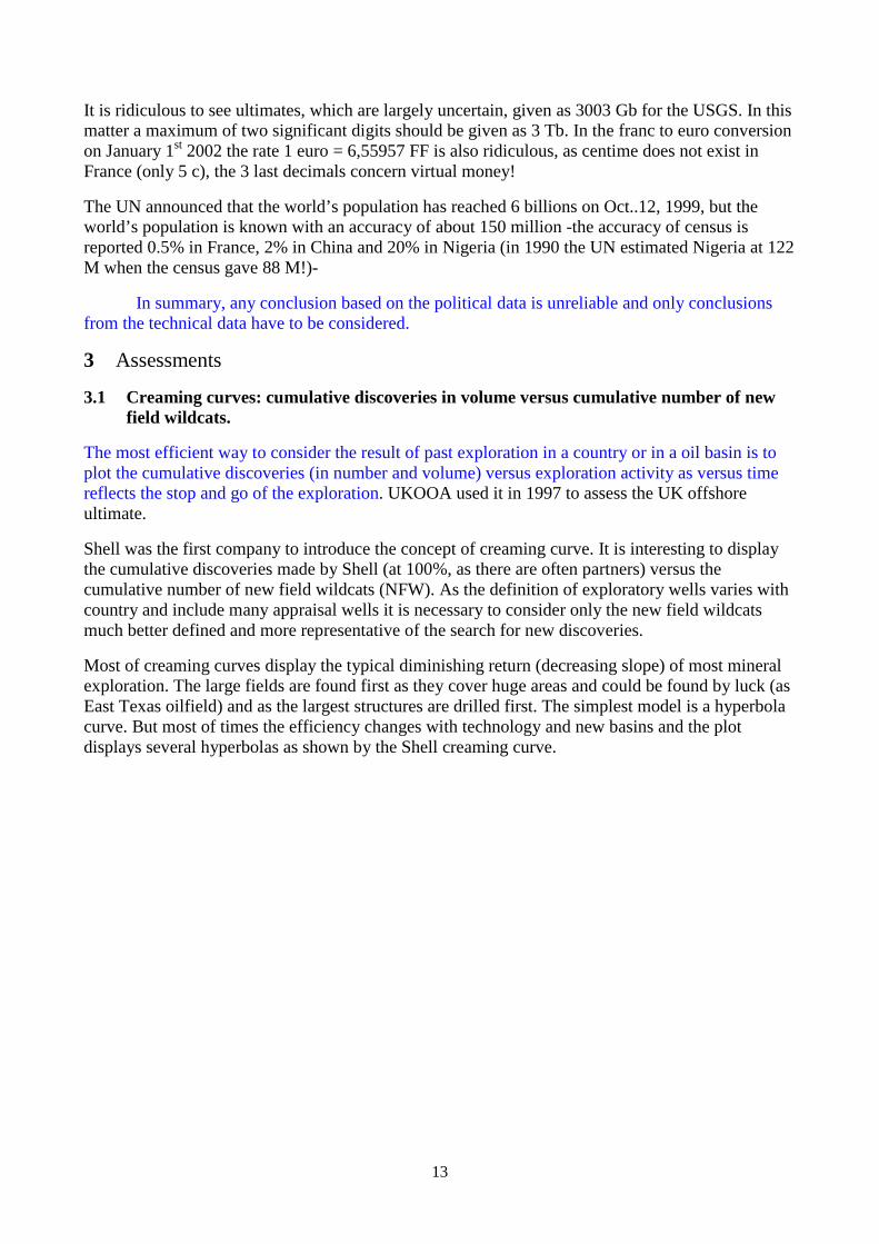
Europe creaming curve can be modelled with two hyperbolas, the second one starting in 1967 withthe offshore exploration.

Figure 7:

Europe oil+condensate: creaming curve

0

20

40

60

80

100

120

0 5000 10000 15000 20000 25000 30000 35000 40000

cumulative number of new field wildcatrs

O+C Gb

cum O Gb

cum G Tcf/10

cum C Gb

model

hyperbola OilU=20 Gb 1900hyperbola OilU=105 Gb 1967

In 2000 with 17 500 NFW, 87 Gb has been found and with 35 000 NFW 115 Gb could be expected.

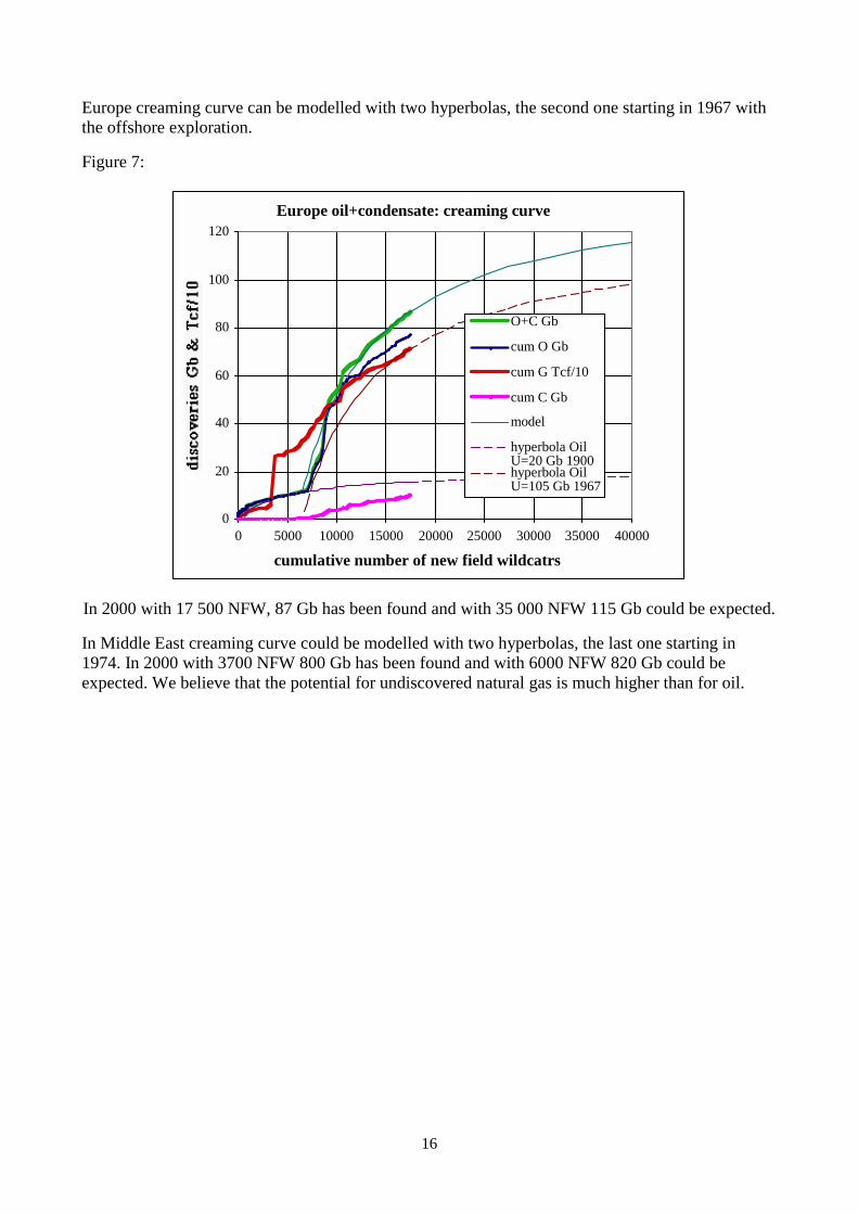
In Middle East creaming curve could be modelled with two hyperbolas, the last one starting in1974. In 2000 with 3700 NFW 800 Gb has been found and with 6000 NFW 820 Gb could beexpected. We believe that the potential for undiscovered natural gas is much higher than for oil.

17

Figure 8:

Middle East oil+condensate: creaming curve

0

100

200

300

400

500

600

700

800

900

0 1000 2000 3000 4000 5000 6000

cumulative number of new field wildcats

disc

over

ies

Gb

&T

cf/1

0 O+C Gb

cum O Gb

cum G Tcf/10

cum C Gb

model

hyperbola U=850 Gb

hyperbola U=130 Gb 1974

North Field& South Pars 1971

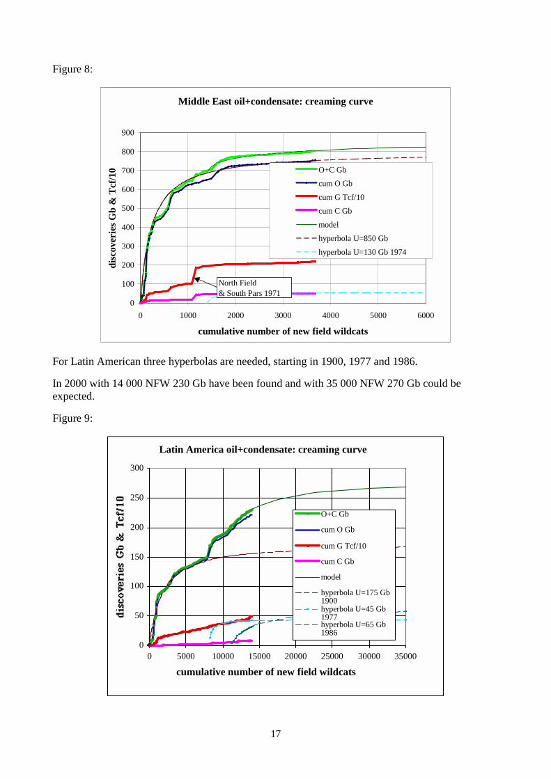
For Latin American three hyperbolas are needed, starting in 1900, 1977 and 1986.

In 2000 with 14 000 NFW 230 Gb have been found and with 35 000 NFW 270 Gb could beexpected.

Figure 9:

Latin America oil+condensate: creaming curve

0

50

100

150

200

250

300

0 5000 10000 15000 20000 25000 30000 35000

cumulative number of new field wildcats

O+C Gb

cum O Gb

cum G Tcf/10

cum C Gb

model

hyperbola U=175 Gb1900hyperbola U=45 Gb1977hyperbola U=65 Gb1986

18

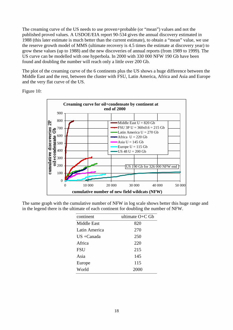
The creaming curve of the US needs to use proven+probable (or “mean”) values and not thepublished proved values. A USDOE/EIA report 90-534 gives the annual discovery estimated in1988 (this later estimate is much better than the current estimate), to obtain a “mean” value, we usethe reserve growth model of MMS (ultimate recovery is 4.5 times the estimate at discovery year) togrow these values (up to 1988) and the new discoveries of annual reports (from 1989 to 1999). TheUS curve can be modelled with one hyperbola. In 2000 with 330 000 NFW 190 Gb have beenfound and doubling the number will reach only a little over 200 Gb.

The plot of the creaming curve of the 6 continents plus the US shows a huge difference between theMiddle East and the rest, between the cluster with FSU, Latin America, Africa and Asia and Europeand the very flat curve of the US.

Figure 10:

Creaming curve for oil+condensate by continent atend of 2000

0

100

200

300

400

500

600

700

800

900

0 10 000 20 000 30 000 40 000 50 000

cumulative number of new field wildcats (NFW)

Middle East U = 820 GbFSU 3P U = 360x0.6 = 215 GbLatin America U = 270 GbAfrica U = 220 GbAsia U = 145 GbEurope U = 115 GbUS 48 U = 200 Gb

US 190 Gb for 326 000 NFW end

The same graph with the cumulative number of NFW in log scale shows better this huge range andin the legend there is the ultimate of each continent for doubling the number of NFW.

continent ultimate O+C Gb

Middle East 820

Latin America 270

US +Canada 250

Africa 220

FSU 215

Asia 145

Europe 115

World 2000

19

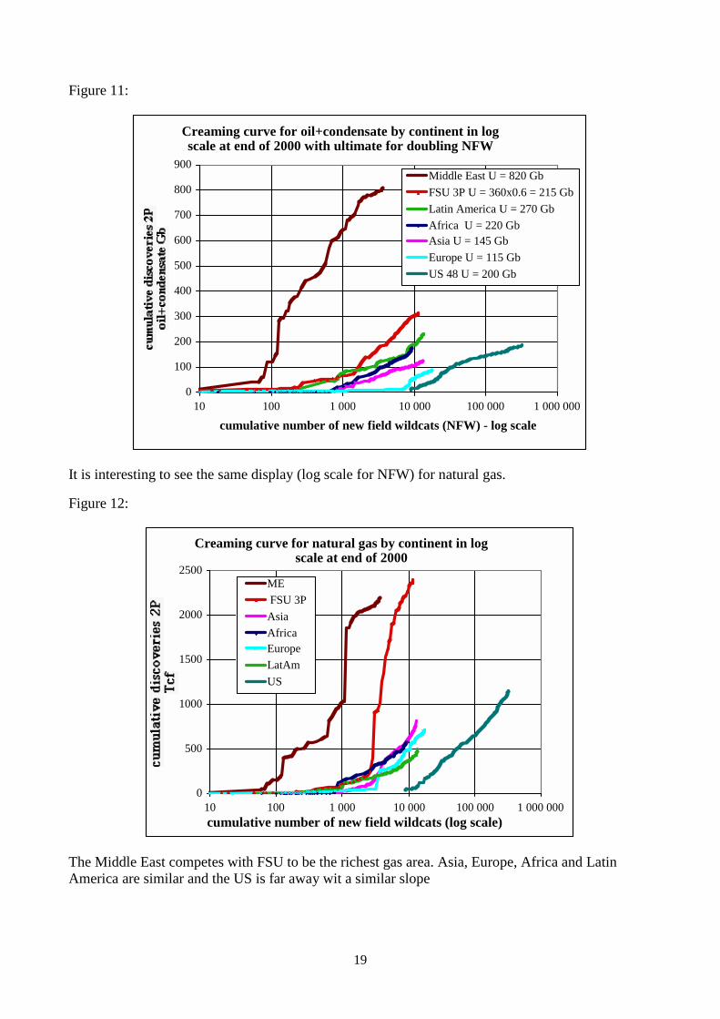
Figure 11:

Creaming curve for oil+condensate by continent in logscale at end of 2000 with ultimate for doubling NFW

0

100

200

300

400

500

600

700

800

900

10 100 1 000 10 000 100 000 1 000 000

cumulative number of new field wildcats (NFW) - log scale

Middle East U = 820 Gb

FSU 3P U = 360x0.6 = 215 Gb

Latin America U = 270 Gb

Africa U = 220 GbAsia U = 145 Gb

Europe U = 115 Gb

US 48 U = 200 Gb

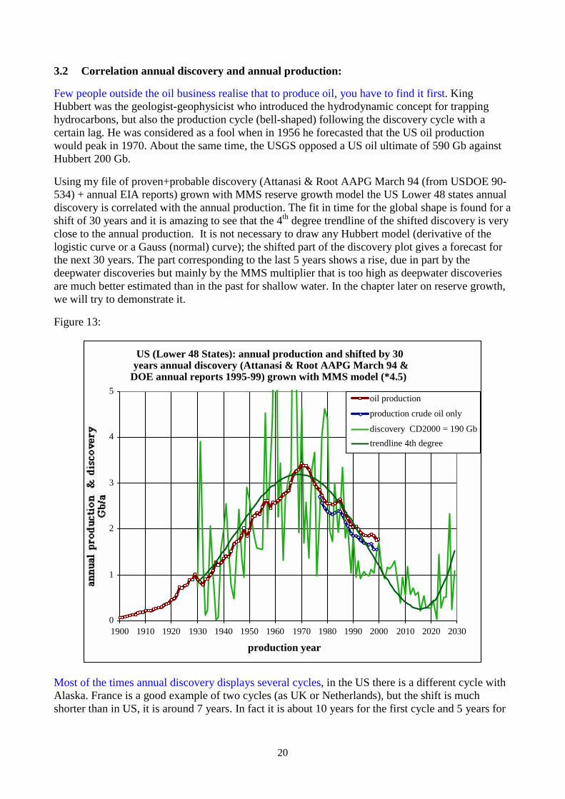
It is interesting to see the same display (log scale for NFW) for natural gas.

Figure 12:

Creaming curve for natural gas by continent in logscale at end of 2000

0

500

1000

1500

2000

2500

10 100 1 000 10 000 100 000 1 000 000cumulative number of new field wildcats (log scale)

ME

FSU 3P

Asia

AfricaEurope

LatAm

US

The Middle East competes with FSU to be the richest gas area. Asia, Europe, Africa and LatinAmerica are similar and the US is far away wit a similar slope

20

3.2 Correlation annual discovery and annual production:

Few people outside the oil business realise that to produce oil, you have to find it first. KingHubbert was the geologist-geophysicist who introduced the hydrodynamic concept for trappinghydrocarbons, but also the production cycle (bell-shaped) following the discovery cycle with acertain lag. He was considered as a fool when in 1956 he forecasted that the US oil productionwould peak in 1970. About the same time, the USGS opposed a US oil ultimate of 590 Gb againstHubbert 200 Gb.

Using my file of proven+probable discovery (Attanasi & Root AAPG March 94 (from USDOE 90-534) + annual EIA reports) grown with MMS reserve growth model the US Lower 48 states annualdiscovery is correlated with the annual production. The fit in time for the global shape is found for ashift of 30 years and it is amazing to see that the 4th degree trendline of the shifted discovery is veryclose to the annual production. It is not necessary to draw any Hubbert model (derivative of thelogistic curve or a Gauss (normal) curve); the shifted part of the discovery plot gives a forecast forthe next 30 years. The part corresponding to the last 5 years shows a rise, due in part by thedeepwater discoveries but mainly by the MMS multiplier that is too high as deepwater discoveriesare much better estimated than in the past for shallow water. In the chapter later on reserve growth,we will try to demonstrate it.

Figure 13:

US (Lower 48 States): annual production and shifted by 30years annual discovery (Attanasi & Root AAPG March 94 &

DOE annual reports 1995-99) grown with MMS model (*4.5)

0

1

2

3

4

5

1900 1910 1920 1930 1940 1950 1960 1970 1980 1990 2000 2010 2020 2030

production year

oil production

production crude oil only

discovery CD2000 = 190 Gb

trendline 4th degree

Most of the times annual discovery displays several cycles, in the US there is a different cycle withAlaska. France is a good example of two cycles (as UK or Netherlands), but the shift is muchshorter than in US, it is around 7 years. In fact it is about 10 years for the first cycle and 5 years for

21

the second cycle. The low value period in time (15 years) between the two cycles is about the samein discovery and production.

Figure 14:

France: annual oil production & annual discovery shiftedby 7 years

0

10

20

30

40

50

1950 1960 1970 1980 1990 2000 2010

year of production

annual discovery CD=925 Mb

annual production CP=737 Mb

FSU being as the US 48 a large country with many oil basins has an annual discovery pattern as abell-shaped curve. The fit in time between the annual discovery and annual production is about 20years but the 4th degree trendline of discovery does not fit with the production curve. But theRussian classification corresponds to proven +probable+possible (or 3P) as reserve estimates weremade using the maximum theoretical recovery factor, neglecting economy and technology, asquoted by Khalimov (1993). The fit is good when the 3P annual discovery is reduced by 45% from1950 to 1990 to correspond to 2P values. During 1990 to 2000 the breakdown of the FSU hasdisturbed the fit. But now the present production is in line with the discovery.

22

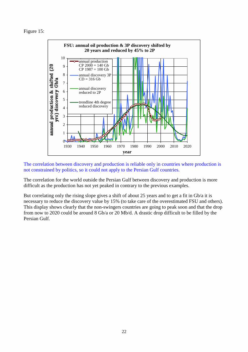
Figure 15:

FSU: annual oil production & 3P discovery shifted by20 years and reduced by 45% to 2P

0

1

2

3

4

5

6

7

8

9

10

1930 1940 1950 1960 1970 1980 1990 2000 2010 2020

year

annual productionCP 2000 = 140 GbCP 1987 = 100 Gb

annual discovery 3PCD = 316 Gb

annual discoveryreduced to 2P

trendline 4th degreereduced discovery

The correlation between discovery and production is reliable only in countries where production isnot constrained by politics, so it could not apply to the Persian Gulf countries.

The correlation for the world outside the Persian Gulf between discovery and production is moredifficult as the production has not yet peaked in contrary to the previous examples.

But correlating only the rising slope gives a shift of about 25 years and to get a fit in Gb/a it isnecessary to reduce the discovery value by 15% (to take care of the overestimated FSU and others).This display shows clearly that the non-swingers countries are going to peak soon and that the dropfrom now to 2020 could be around 8 Gb/a or 20 Mb/d. A drastic drop difficult to be filled by thePersian Gulf.

23

Figure 16:

World outside the swing producers (Persian Gulf): annualproduction & annual discovery shifted by 25 years & reduced

by 15%

0

5

10

15

20

25

30

1930 1940 1950 1960 1970 1980 1990 2000 2010 2020 2030

production year

production

trendline discovery 4th degree

discovery shiftedby 25 years &

reduced by 15%

The WEC 2000 “Energy for tomorrow’s world –Acting Now » has already shown (page 80 & 81) mygraphs of US and world outside the swing producers discovery-production, but the above graphs areupdated to 2001.

3.3 Parabolic fractal display:

One of the best displays is the fractal distribution of field size-rank in a log-log format. When thedistribution is natural as it is in a Petroleum System the fractal displays follow a curve (and not astraight line (or power law) as claimed by Mandelbrot) (Laherrere 1996, 1999). This parabolicfractal is found for urban agglomerations, earthquake (the Ritcher-Gutenberg, power law, is a roughapproximation), galaxies, species, . A fractal distribution corresponds to auto-similarity, quitefrequent in nature, but as auto-similarity is not perfect, the fractal is not linear, but curved.

24

Figure 17:

Niger delta: oilfield size fractal display

1

10

100

1000

10000

1 10 100 1000

rank

up to 1959up to 1969up to 1979up to 1989up to 2000

The parabolic fractal display of the Niger delta Petroleum System has just shifted in parallel from1993 to 2000. Revisions and new discoveries do not change the distribution, it increases globallythe reserves.

25

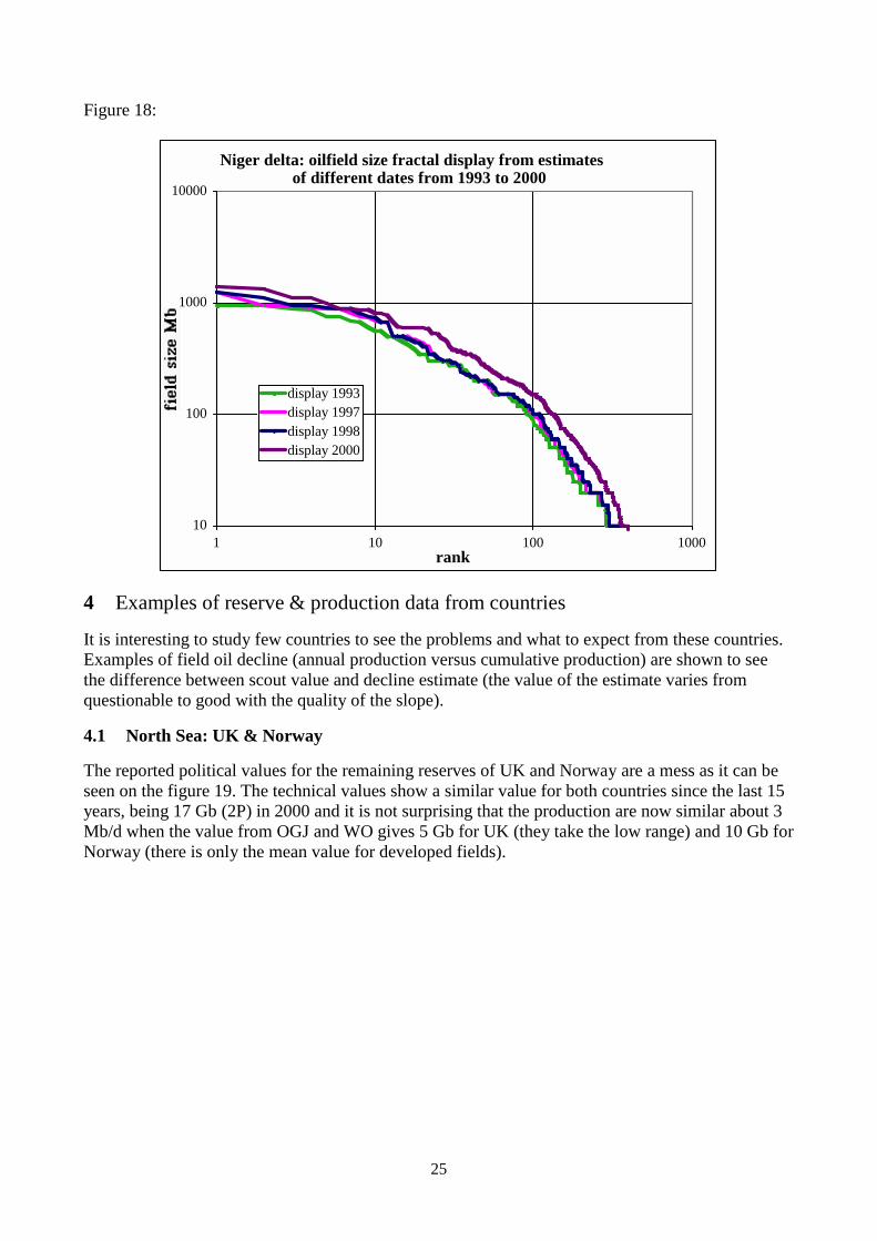
Figure 18:

Niger delta: oilfield size fractal display from estimatesof different dates from 1993 to 2000

10

100

1000

10000

1 10 100 1000rank

display 1993display 1997display 1998display 2000

4 Examples of reserve & production data from countries

It is interesting to study few countries to see the problems and what to expect from these countries.Examples of field oil decline (annual production versus cumulative production) are shown to seethe difference between scout value and decline estimate (the value of the estimate varies fromquestionable to good with the quality of the slope).

4.1 North Sea: UK & Norway

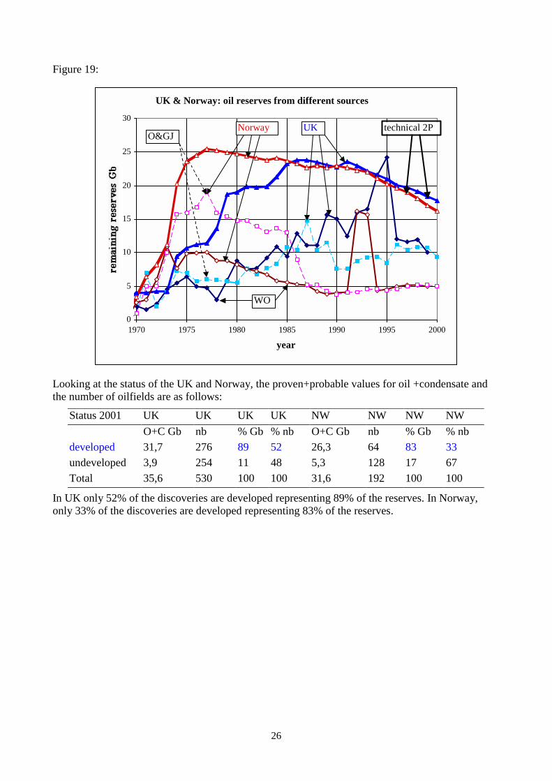
The reported political values for the remaining reserves of UK and Norway are a mess as it can beseen on the figure 19. The technical values show a similar value for both countries since the last 15years, being 17 Gb (2P) in 2000 and it is not surprising that the production are now similar about 3Mb/d when the value from OGJ and WO gives 5 Gb for UK (they take the low range) and 10 Gb forNorway (there is only the mean value for developed fields).

26

Figure 19:

UK & Norway: oil reserves from different sources

0

5

10

15

20

25

30

1970 1975 1980 1985 1990 1995 2000

year

Norway UKO&GJ

WO

technical 2P

Looking at the status of the UK and Norway, the proven+probable values for oil +condensate andthe number of oilfields are as follows:

Status 2001 UK UK UK UK NW NW NW NW

O+C Gb nb % Gb % nb O+C Gb nb % Gb % nb

developed 31,7 276 89 52 26,3 64 83 33

undeveloped 3,9 254 11 48 5,3 128 17 67

Total 35,6 530 100 100 31,6 192 100 100

In UK only 52% of the discoveries are developed representing 89% of the reserves. In Norway,only 33% of the discoveries are developed representing 83% of the reserves.

27

Figure 20:

UK & Norway annual production & shifted annual discovery

0

0,5

1

1,5

2

2,5

3

1970 1980 1990 2000 2010 2020

production year

UK discovery CD=36 Gbshifted 10 yearsUK production CP=20 Gb

NW discovery CD=32 Gbshifted 20 yearsNW production CP=14 Gb

The oil decline of Forties is easy to extrapolate. The Brown Book agrees with the decline.

Figure 21:

Forties oil decline

0

20

40

60

80

100

120

140

160

180

200

0 500 1000 1500 2000 2500 3000

cumulative production Mb

an prod before declinean prod since 1985ultimate Brown 2000ultimate decline

forecast 2001-2010Wood MacKenzie

5th platform & gasliftincrease productionfor 2 years but not ultimate

28

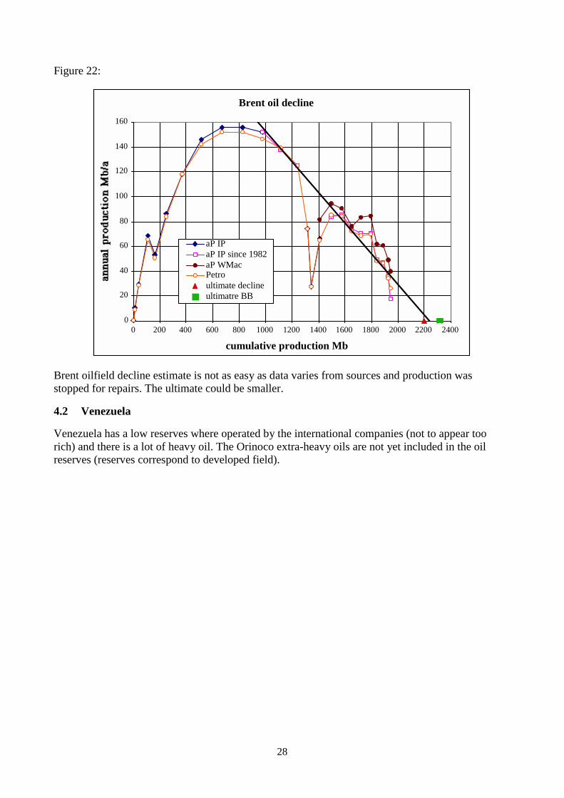
Figure 22:

Brent oil decline

0

20

40

60

80

100

120

140

160

0 200 400 600 800 1000 1200 1400 1600 1800 2000 2200 2400

cumulative production Mb

aP IPaP IP since 1982aP WMacPetroultimate declineultimatre BB

Brent oilfield decline estimate is not as easy as data varies from sources and production wasstopped for repairs. The ultimate could be smaller.

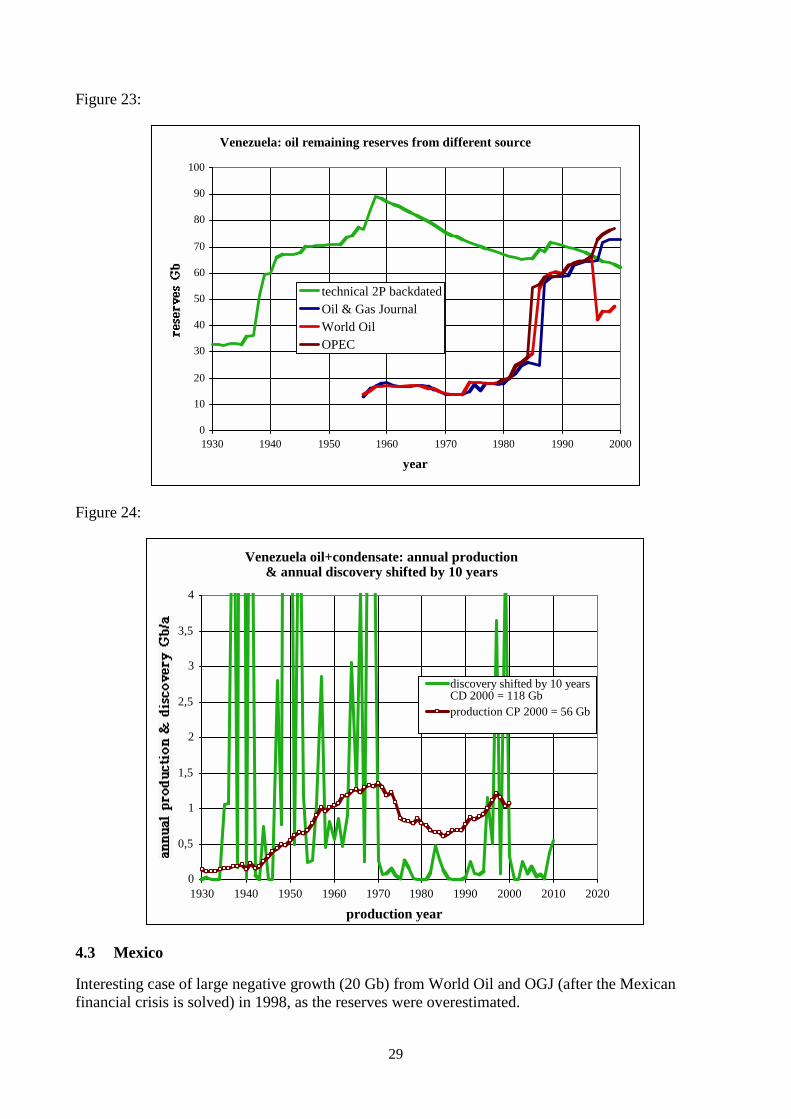
4.2 Venezuela

Venezuela has a low reserves where operated by the international companies (not to appear toorich) and there is a lot of heavy oil. The Orinoco extra-heavy oils are not yet included in the oilreserves (reserves correspond to developed field).

29

Figure 23:

Venezuela: oil remaining reserves from different source

0

10

20

30

40

50

60

70

80

90

100

1930 1940 1950 1960 1970 1980 1990 2000

year

technical 2P backdatedOil & Gas JournalWorld OilOPEC

Figure 24:

Venezuela oil+condensate: annual production& annual discovery shifted by 10 years

0

0,5

1

1,5

2

2,5

3

3,5

4

1930 1940 1950 1960 1970 1980 1990 2000 2010 2020

production year

discovery shifted by 10 yearsCD 2000 = 118 Gbproduction CP 2000 = 56 Gb

4.3 Mexico

Interesting case of large negative growth (20 Gb) from World Oil and OGJ (after the Mexicanfinancial crisis is solved) in 1998, as the reserves were overestimated.

30

Figure 25:

Mexico: remaining oil reserves from different sources

0

10

20

30

40

50

60

1930 1940 1950 1960 1970 1980 1990 2000

year

technical 2P backdatedOil & G&s JournalWorld Oil

Figure 26:

Mexico: anual oil production & annual discoveryshifted by 5 years

0

0,5

1

1,5

2

2,5

3

3,5

4

4,5

5

1910 1920 1930 1940 1950 1960 1970 1980 1990 2000 2010

year of production

discovery CD2000 = 56 Gb

production CP = 28 Gb

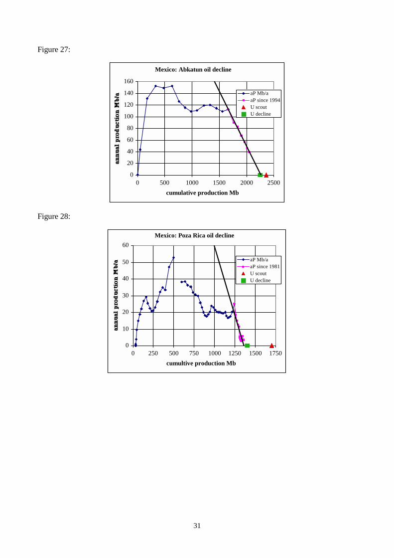
The largest field Cantarell is not yet on decline with EOR investments. But most other fields are ondecline.

31

Figure 27:

Mexico: Abkatun oil decline

0

20

40

60

80

100

120

140

160

0 500 1000 1500 2000 2500

cumulative production Mb

aP Mb/aaP since 1994U scoutU decline

Figure 28:

Mexico: Poza Rica oil decline

0

10

20

30

40

50

60

0 250 500 750 1000 1250 1500 1750

cumultive production Mb

aP Mb/aaP since 1981U scoutU decline

32

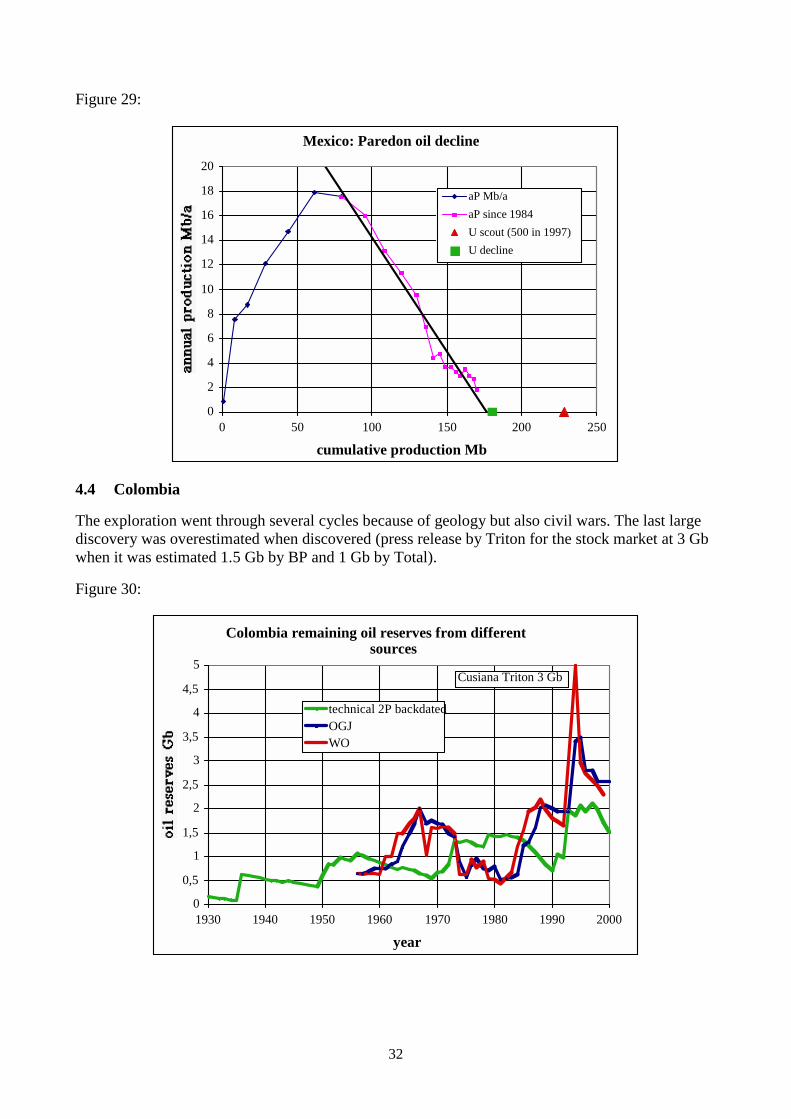
Figure 29:

Mexico: Paredon oil decline

0

2

4

6

8

10

12

14

16

18

20

0 50 100 150 200 250

cumulative production Mb

aP Mb/a

aP since 1984

U scout (500 in 1997)

U decline

4.4 Colombia

The exploration went through several cycles because of geology but also civil wars. The last largediscovery was overestimated when discovered (press release by Triton for the stock market at 3 Gbwhen it was estimated 1.5 Gb by BP and 1 Gb by Total).

Figure 30:

Colombia remaining oil reserves from differentsources

0

0,5

1

1,5

2

2,5

3

3,5

4

4,5

5

1930 1940 1950 1960 1970 1980 1990 2000

year

technical 2P backdatedOGJWO

Cusiana Triton 3 Gb

33

Figure 31:

Colombia annual oil production & annual discoveryshifted by 5 years

0

0,05

0,1

0,15

0,2

0,25

0,3

0,35

0,4

0,45

0,5

1930 1940 1950 1960 1970 1980 1990 2000 2010

production year

discovery CD2000 = 9,3 Gb

production CP2000 = 5,3 Gb

The Cusiana field has started to decline (last year) and the estimate is now about 700 Mb, when the“scout” value is 950 Mb (but 1625 Mb last year).

Figure 32:

Colombia Cusiana oil decline

0

10

20

30

40

50

60

70

80

90

100

0 100 200 300 400 500 600 700 800 900 1000cumulative production Mb

aP

aP since 1999

U scout 950 Mb(1625 in 1999)U decline 700 Mb ?

34

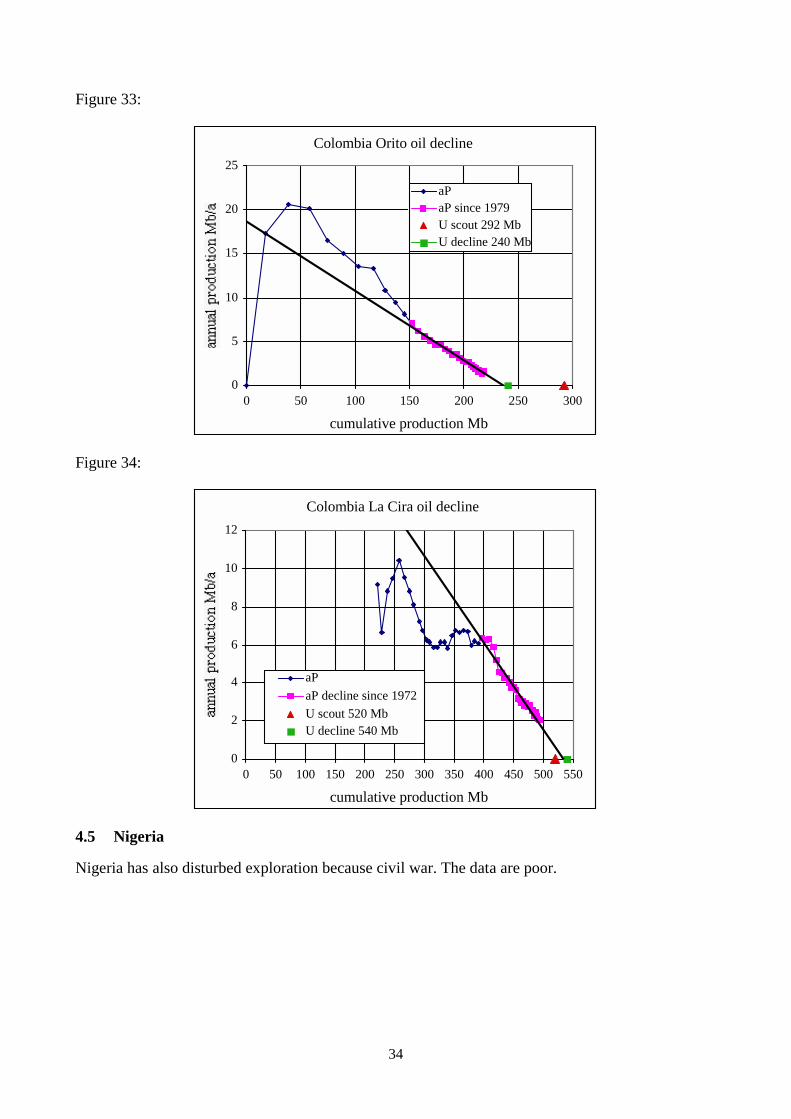
Figure 33:

Colombia Orito oil decline

0

5

10

15

20

25

0 50 100 150 200 250 300

cumulative production Mb

aPaP since 1979U scout 292 MbU decline 240 Mb

Figure 34:

Colombia La Cira oil decline

0

2

4

6

8

10

12

0 50 100 150 200 250 300 350 400 450 500 550

cumulative production Mb

aP

aP decline since 1972

U scout 520 MbU decline 540 Mb

4.5 Nigeria

Nigeria has also disturbed exploration because civil war. The data are poor.

35

Figure 35:

Nigeria: oil remaining reserves from different sources

0

5

10

15

20

25

30

35

1950 1960 1970 1980 1990 2000

year

technical 2P backdatedOil & Gas JournalWorld OilOPEC

Figure 36:

Nigeria: annual oil production & annual discoveryshifted by 10 years

0

0,5

1

1,5

2

2,5

3

3,5

4

4,5

1960 1970 1980 1990 2000 2010 2020

production year

discovery CD= 50 Gb

production CP = 21 Gb

36

Figure 37:

Nigeria: Bomu oil decline

0

5

10

15

20

25

30

0 100 200 300 400 500 600 700

cumulative production Mb

aPaP declineU scoutU decline

4.6 China

Data are not very good and fields are grouped.

37

Figure 38:

China: remaining oil reserves from different sources

0

5

10

15

20

25

30

35

40

1950 1960 1970 1980 1990 2000

year

technical 2P backdated

Oil & Gas Journal

World Oil

The largest oilfield Daqing is very large with a large town to produce it with over 20 000 wells for 1Mb/d.

Figure 39:

China: annual oil production & anuual discovery shiftedby 20 years

0

0,5

1

1,5

2

2,5

3

3,5

4

4,5

1960 1970 1980 1990 2000 2010 2020

production year

discovery shifted 20 years CD2000 = 54 Gb

production CP2000 = 27 Gb

38

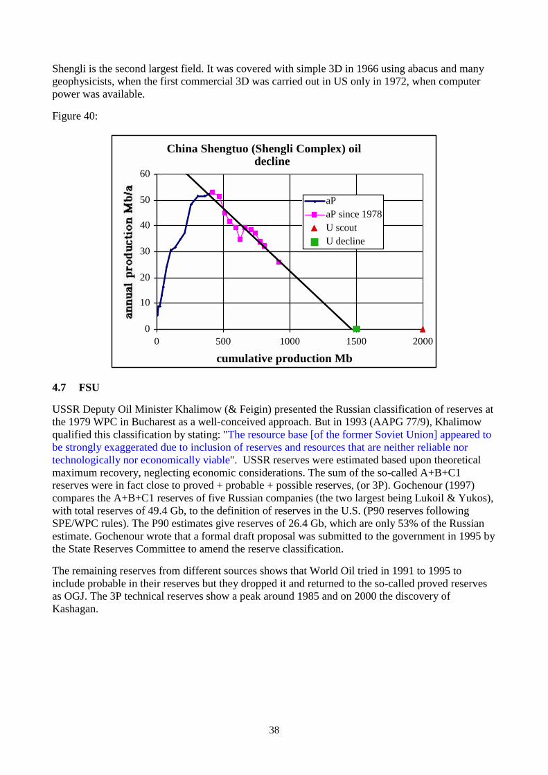
Shengli is the second largest field. It was covered with simple 3D in 1966 using abacus and manygeophysicists, when the first commercial 3D was carried out in US only in 1972, when computerpower was available.

Figure 40:

China Shengtuo (Shengli Complex) oildecline

0

10

20

30

40

50

60

0 500 1000 1500 2000

cumulative production Mb

aPaP since 1978U scoutU decline

4.7 FSU

USSR Deputy Oil Minister Khalimow (& Feigin) presented the Russian classification of reserves atthe 1979 WPC in Bucharest as a well-conceived approach. But in 1993 (AAPG 77/9), Khalimowqualified this classification by stating: "The resource base [of the former Soviet Union] appeared tobe strongly exaggerated due to inclusion of reserves and resources that are neither reliable nortechnologically nor economically viable". USSR reserves were estimated based upon theoreticalmaximum recovery, neglecting economic considerations. The sum of the so-called A+B+C1reserves were in fact close to proved + probable + possible reserves, (or 3P). Gochenour (1997)compares the A+B+C1 reserves of five Russian companies (the two largest being Lukoil & Yukos),with total reserves of 49.4 Gb, to the definition of reserves in the U.S. (P90 reserves followingSPE/WPC rules). The P90 estimates give reserves of 26.4 Gb, which are only 53% of the Russianestimate. Gochenour wrote that a formal draft proposal was submitted to the government in 1995 bythe State Reserves Committee to amend the reserve classification.

The remaining reserves from different sources shows that World Oil tried in 1991 to 1995 toinclude probable in their reserves but they dropped it and returned to the so-called proved reservesas OGJ. The 3P technical reserves show a peak around 1985 and on 2000 the discovery ofKashagan.

39

Figure 41:

FSU remaining oil reserves from different sources

0

20

40

60

80

100

120

140

160

180

200

1950 1960 1970 1980 1990 2000

year

technical 2P backdated

OGJ

WO

The fit of the peak of 3P annual discovery to the annual production peak shows a shift of about 20years, but it is necessary to reduce the annual discovery by 45% to get a fit to the level of annualproduction. This reduction is in line with Khalimov’s statement.

Figure 42:

FSU: annual oil production & 3P discovery shifted by20 years and reduced by 45% to 2P

0

1

2

3

4

5

6

7

8

9

10

1930 1940 1950 1960 1970 1980 1990 2000 2010 2020

year

annual productionCP 2000 = 140 GbCP 1987 = 100 Gb

annual discovery 3PCD = 316 Gb

annual discoveryreduced to 2P

trendline 4th degreereduced discovery

40

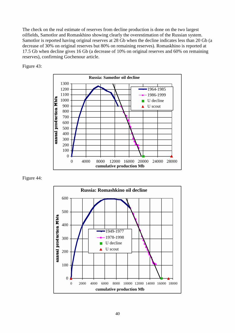
The check on the real estimate of reserves from decline production is done on the two largestoilfields, Samotlor and Romaskhino showing clearly the overestimation of the Russian system.Samotlor is reported having original reserves at 28 Gb when the decline indicates less than 20 Gb (adecrease of 30% on original reserves but 80% on remaining reserves). Romaskhino is reported at17.5 Gb when decline gives 16 Gb (a decrease of 10% on original reserves and 60% on remainingreserves), confirming Gochenour article.

Figure 43:

Russia: Samotlor oil decline

0100200300400500600700800900

1000110012001300

0 4000 8000 12000 16000 20000 24000 28000cumulative production Mb

1964-19851986-1999U declineU scout

Figure 44:

Russia: Romashkino oil decline

0

100

200

300

400

500

600

0 2000 4000 6000 8000 10000 12000 14000 16000 18000

cumulative production Mb

1949-1977

1978-1998U decline

U scout

41

4.8 Oman

Oman is an interesting country as most of oil exploration and production was conducted by PDO, infact Shell, which has run Oman as the best school for its engineers. Shell is the most importantenterprise of the country and Shell manager was as important as the oil minister. I went to Oman (aspartner) and I learned a lot from Shell operations. Oil is produced even in Infracambrian formations.

Figure 45:

Oman: remaining oil reserves from different sources

0

2

4

6

8

10

12

1950 1960 1970 1980 1990 2000

year

technical 2P backdatedOGJWO

42

Figure 46:

Oman annual oil production &discovery shifted by 7 years

0

100

200

300

400

500

600

700

800

900

1000

1960 1970 1980 1990 2000 2010

production year

discovery CD2000 = 13 Gb

production CP2000 = 6,4 Gb

The Fahud field discovered in 1964 is interesting, as it is located 200 meter from a dry hole drilledin 1957 by the IPC consortium that decided to drop exploration except Shell (and Gulbenkian).

Figure 47:

Oman Fahud (1964) oil decline

0

10

20

30

40

50

60

70

80

0 200 400 600 800 1000 1200cumulative production Mb

aPaP sinceU declineU scout

43

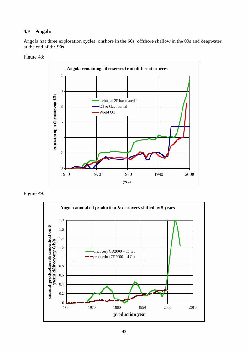
4.9 Angola

Angola has three exploration cycles: onshore in the 60s, offshore shallow in the 80s and deepwaterat the end of the 90s.

Figure 48:

Angola remaining oil reserves from different sources

0

2

4

6

8

10

12

1960 1970 1980 1990 2000

year

technical 2P backdated

Oil & Gas Journal

World Oil

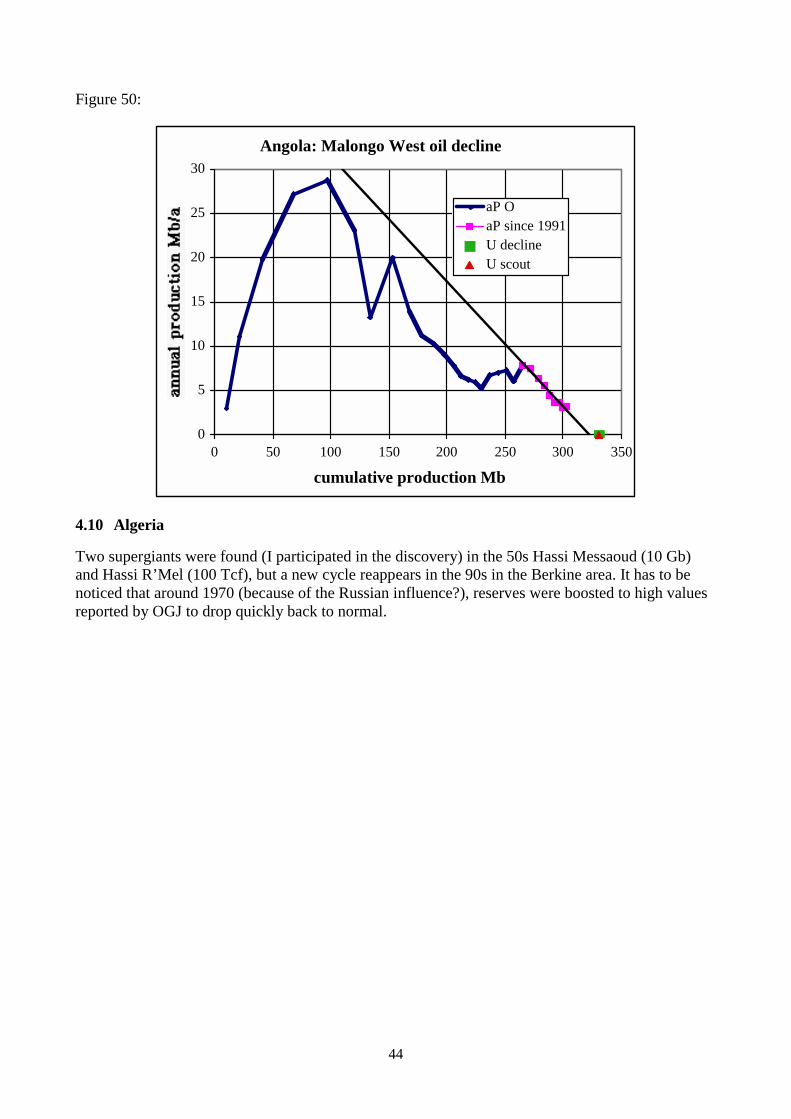
Figure 49:

Angola annual oil production & discovery shifted by 5 years

0

0,2

0,4

0,6

0,8

1

1,2

1,4

1,6

1,8

1960 1970 1980 1990 2000 2010

production year

discovery CD2000 = 15 Gb

production CP2000 = 4 Gb

44

Figure 50:

Angola: Malongo West oil decline

0

5

10

15

20

25

30

0 50 100 150 200 250 300 350

cumulative production Mb

aP OaP since 1991U declineU scout

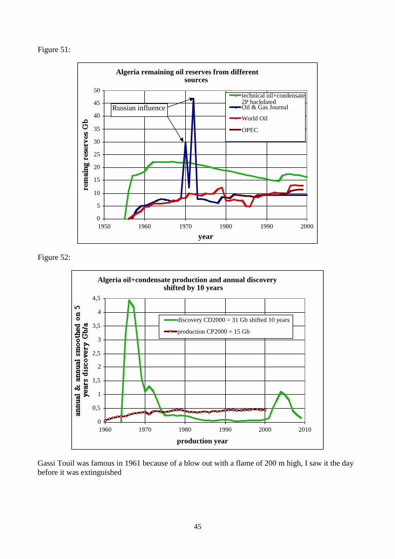
4.10 Algeria

Two supergiants were found (I participated in the discovery) in the 50s Hassi Messaoud (10 Gb)and Hassi R’Mel (100 Tcf), but a new cycle reappears in the 90s in the Berkine area. It has to benoticed that around 1970 (because of the Russian influence?), reserves were boosted to high valuesreported by OGJ to drop quickly back to normal.

45

Figure 51:

Algeria remaining oil reserves from differentsources

0

5

10

15

20

25

30

35

40

45

50

1950 1960 1970 1980 1990 2000

year

technical oil+condensate2P backdatedOil & Gas Journal

World Oil

OPEC

Russian influence

Figure 52:

Algeria oil+condensate production and annual discoveryshifted by 10 years

0

0,5

1

1,5

2

2,5

3

3,5

4

4,5

1960 1970 1980 1990 2000 2010

production year

discovery CD2000 = 31 Gb shifted 10 years

production CP2000 = 15 Gb

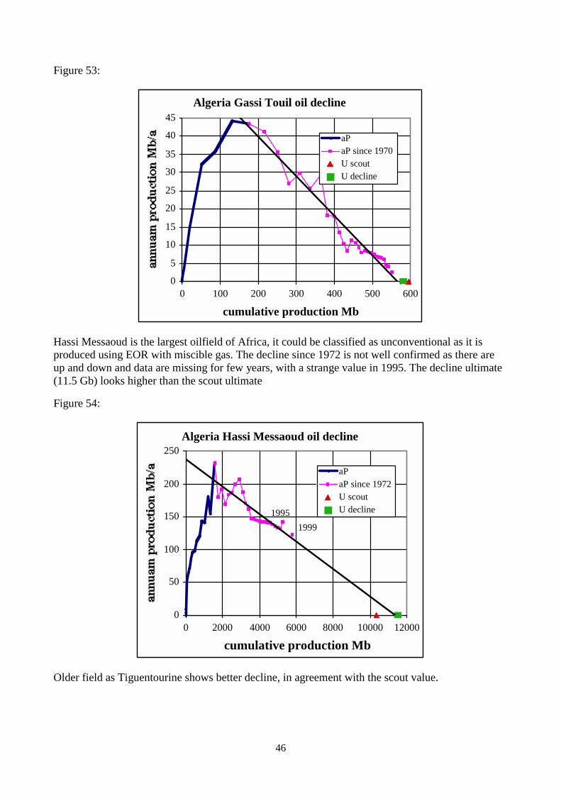
Gassi Touil was famous in 1961 because of a blow out with a flame of 200 m high, I saw it the daybefore it was extinguished

46

Figure 53:

Algeria Gassi Touil oil decline

0

5

10

15

20

25

30

35

40

45

0 100 200 300 400 500 600

cumulative production Mb

aPaP since 1970U scoutU decline

Hassi Messaoud is the largest oilfield of Africa, it could be classified as unconventional as it isproduced using EOR with miscible gas. The decline since 1972 is not well confirmed as there areup and down and data are missing for few years, with a strange value in 1995. The decline ultimate(11.5 Gb) looks higher than the scout ultimate

Figure 54:

Algeria Hassi Messaoud oil decline

0

50

100

150

200

250

0 2000 4000 6000 8000 10000 12000

cumulative production Mb

aPaP since 1972U scoutU decline1995

1999

Older field as Tiguentourine shows better decline, in agreement with the scout value.

47

Figure 55

Algeria Tiguentourine oil decline

0

1

2

3

4

5

0 20 40 60 80 100

cumulative production Mb

aP O+CaP declineU declineU scout

5 Reserve growth

Reserve growth is the most important problem in assessing the future production.

Statistically reserve growth occurs because the reserves are badly estimated. If they were estimatedwith a probabilistic approach using a wide range of minimum, mean, maximum, statistically themean reserves of a country is the sum of the mean reserves of each - which is not the case forProved Reserves - and there should not be any global growth in the day of reckoning at the end ofproduction of the country, despite huge variation in detail between estimated value and real value ofevery field.

At the present time, it is claimed that there is reserve growth in the evolution of the reserves, but infact the extent of reserve growth can be measured only when the fields have been depleted andabandoned. On still producing fields, cases of reserve growth are publicised whereas little is saidabout reserve decrease. The huge increase during the second half of the 1980s by the OPECcountries was political (quotas) and the decrease in 1999 of 20 Gb by Mexico was done after thefinancial crisis was solved (previously large reserves were needed to guarantee the loan from theUS and IMF and before Nafta agreement signed)

Reserve growth is claimed to come from higher recovery factor thanks to technology progress andincrease in oil price. Is it true?

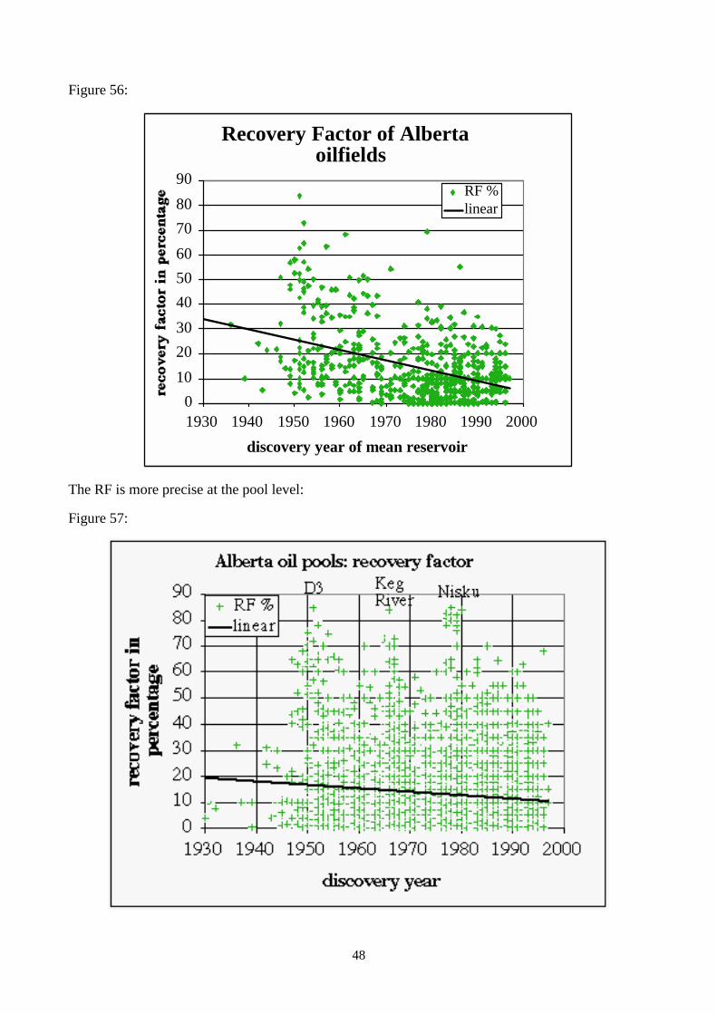
5.1 Recovery factor (RF)

People believe that the recovery factor is a function of the technology level when it is mainly due togeology, to the quality of the reservoir and not the quality of the production scheme or the presenttechnology. It is obvious in Canada that the RF varies with time not with technology but with thedifferent types of reefs found when exploration moves to a new area and new play.

48

Figure 56:

Recovery Factor of Albertaoilfields

0

10

20

30

40

50

60

70

80

90

1930 1940 1950 1960 1970 1980 1990 2000

discovery year of mean reservoir

RF %linear

The RF is more precise at the pool level:

Figure 57:

49

It is known that for poor reservoirs (fractured tight reservoir) the RF is about 3% and for very highporous and permeable reservoir (as a reef) it is about 80%.

5.2 Geology mainly

In the North Sea the distribution of cumulative discoveries versus RF shows an almost identicalcurve between UK and Norway. As most of the reserves comes from North Sea and since theboundaries is at the middle of distance, having identical distribution the reserves are evenly spreadin the North Sea, the largest being close to the centre (Viking grabens). It is funny to think the limitbetween the two nations were settled using the middle distance, giving half of the reserves to eachcountries. Another rule could have been chosen as the deepest waters, giving nothing to Norway, asthe country is only basement and the deepest water line stays in the basement. It could be said that itis unfair to give a sedimentary offshore to a country with a basement onshore and offshore up to thedeepest waters.

Figure 58:

Cumulative oil reserves versus oil recovery factor forUK and Norway

0

5

10

15

20

25

30

0 10 20 30 40 50 60 70 80

oil recovery factor %

NWUK

RF varies from 20% to 40% (5%-95%) with the median reserves around 45%. Norway has decidedin 1999 to take 50% as the goal for average oil reserves.

The distribution by continent on figure shows different pattern for the percentage of reserve versusRF. The best one is for Australiasia and the worst for Latin America.

50

Figure 59:

Percentage of cumulative oil discoveries versus oilrecovery factor

0

10

20

30

40

50

60

70

80

90

100

0 10 20 30 40 50 60 70 80

oil recovery factor %

ME 734 reportedout of 754 GbCIS 50 Gb out of290 GbLatAm 208 Gbout of 221 GbAfrica 156 Gbout of 160 GbFar East 96 Gbout of 106 GbEurope 66 Gbout of 72 GbAustralAsia 7.2Gb of 7.6Gb

The median point 550% of the reserves is at 30% for Latin America, 33% for Middle East, 40% forAfrica, Far East and Europe, 45% for CIS and 55% for AustralAsia.

The same graph for gas recovery factor (range RF 50%-90%) shows a median point at 70% forLatin America, 75% for the rest. (Norway has chosen 75% as its goal average).

51

Figure 60:

Percentage of cumulative gas discoveries versus gas recoveryfactor

0

10

20

30

40

50

60

70

80

90

100

0 10 20 30 40 50 60 70 80 90 100

gas recovery factor %

CIS 84 Tcf reported RF out of 2403 Tcf

Middle East 1489 of 2195 Tcf

Far East 496 of 624 Tcf

Europe 468 of 604 Tcf

Africa 356 of 572 Tcf

LatAm 365 of 496 Tcf

AustralAsia 178 of 189 Tcf

The main impact of technology progress on conventional fields is to produce cheaper, faster but notmore.

The best example is the giant oilfield of Forties in North Sea. The operator announced that thereserves would increase thanks to a fifth platform with gas injection in 1985. The annual productionin 1986 & 1987 were larger than the past decline but in 1988 the production went back to the pastdecline on the same ultimate as before. The estimates from the Brown Book (DTI) do not give thebest values that can be assessed from the technical data.

52

Figure 61:

Forties oilfield: evolution reserves from Brown Book

0

500

1000

1500

2000

2500

3000

1975 1980 1985 1990 1995 2000 2005 2010

year

ultimates Brown Book

ultimate from decline since 1986

cumulative production with WoodMacKenzie forecast 2001-2010

From the decline graph annual production versus cumulative production it is obvious that theultimate was established as earlier than 1986 at 2.7 Gb but the operator waited until 1997 to reportthis value.

Figure 62:

Forties oil decline

0

20

40

60

80

100

120

140

160

180

200

0 500 1000 1500 2000 2500 3000

cumulative production Mb

an prod before declinean prod since 1985ultimate Brown 2000ultimate decline

forecast 2001-2010Wood MacKenzie

5th platform & gasliftincrease productionfor 2 years but not ultimate

53

The reported ultimate for Thistle varies up and down from 1980 to 1996, when the ultimate couldbe correctly estimated at 410 Mb since 1983.

Figure 63:

Thistle oilfield: evolution reserves from Brown Book

0

100

200

300

400

500

600

1975 1980 1985 1990 1995 2000 2005

year

ultimate Brown Book

ultimate from decline since 1983

cumulative production with WoodMackenzie forecast 2001-2003

Figure 64:

Thistle oil decline

0

5

10

15

20

25

30

35

40

45

50

0 50 100 150 200 250 300 350 400 450

cumulative production Mb

an prod before declinean prod since 1982ultimate Brown Book 2000ultimate decline

forecast 2001-2003Wood MacKenzie

54

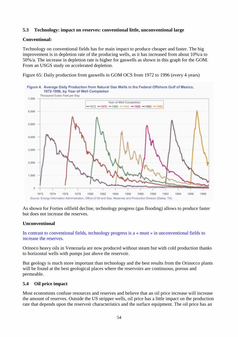
5.3 Technology: impact on reserves: conventional little, unconventional large

Conventional:

Technology on conventional fields has for main impact to produce cheaper and faster. The bigimprovement is in depletion rate of the producing wells, as it has increased from about 10%/a to50%/a. The increase in depletion rate is higher for gaswells as shown in this graph for the GOM.From an USGS study on accelerated depletion.

Figure 65: Daily production from gaswells in GOM OCS from 1972 to 1996 (every 4 years)

As shown for Forties oilfield decline, technology progress (gas flooding) allows to produce fasterbut does not increase the reserves.

Unconventional

In contrast to conventional fields, technology progress is a « must » in unconventional fields toincrease the reserves.

Orinoco heavy oils in Venezuela are now produced without steam but with cold production thanksto horizontal wells with pumps just above the reservoir.

But geology is much more important than technology and the best results from the Orinocco plantswill be found at the best geological places where the reservoirs are continuous, porous andpermeable.

5.4 Oil price impact

Most economists confuse resources and reserves and believe that an oil price increase will increasethe amount of reserves. Outside the US stripper wells, oil price has a little impact on the productionrate that depends upon the reservoir characteristics and the surface equipment. The oil price has an

55

effect on the decision to drill or not marginal prospects, but not on the production except for infilledwells and stripper wells which are classified as unconventional oil. Usually high oil pricescorrespond to a decrease in success ratio, as poor prospects are drilled.

Most of the misunderstanding on this point comes that the economists treat oil and gas fields asmineral deposits as coal, copper, gold or uranium. The production of a mine depends of theeconomical cut-off and the low concentrated ores are treated as wastes. When the price of themineral increases the low-grade ores are considered as new reserves. In case of oil, oil is liquid andit is produced directly without needing any concentration plant (water is simply eliminated), it iseven better for gas. An oilfield is already concentrated deposit and does not need to be concentratedfurther, it is drilled, capped and when flowing it is only necessary to open the tap to produce it.

Furthermore economists consider only the money involved, omitting to look at the “net energy” orthe energy return on invested energy. The net energy can be negative as it is often for the ethanolfrom corns.

5.5 Difference between old fields and new fields

Reserve growth analysis has to be performed using data on modern discoveries in order to properlyextrapolate estimated reserves to the future. Most of the reserve growth in the Lower 48 statescomes from Californian heavy oilfields found a century ago, with the Midway-Sunset oil fieldshown to be the best example of reserve growth by Schmoker USGS 2000 FS 119-00. The MineralsManagement Service (MMS) has elaborated a model for the Gulf of Mexico (GOM) and theirreserve growth curve is only about half of the Lower 48 reserve growth function used for the worldoutside the US in the USGS 2000 assessment. The 1999 Annual Report by the US DOE/EIA givespositive reserve additions for the federal GOM (Louisiana) of 693 Mb and negative revisions of 730Mb. They also report 2 Mb for adjustments, 55 Mb for extensions, 238 Mb for new field discoveriesand 77 Mb for new reservoirs in old fields, 376 Mb for production and proved reserves went from2483 Mb in 1998 to 2442 Mb in 1999. For this area, the negative revisions were larger than thepositive revisions in 1999 (in 1998 they were about the same) which means that reserve growthcould be about zero for the GOM where 78% of the oil was discovered before 1980.

5.6 Poor and contradictory data

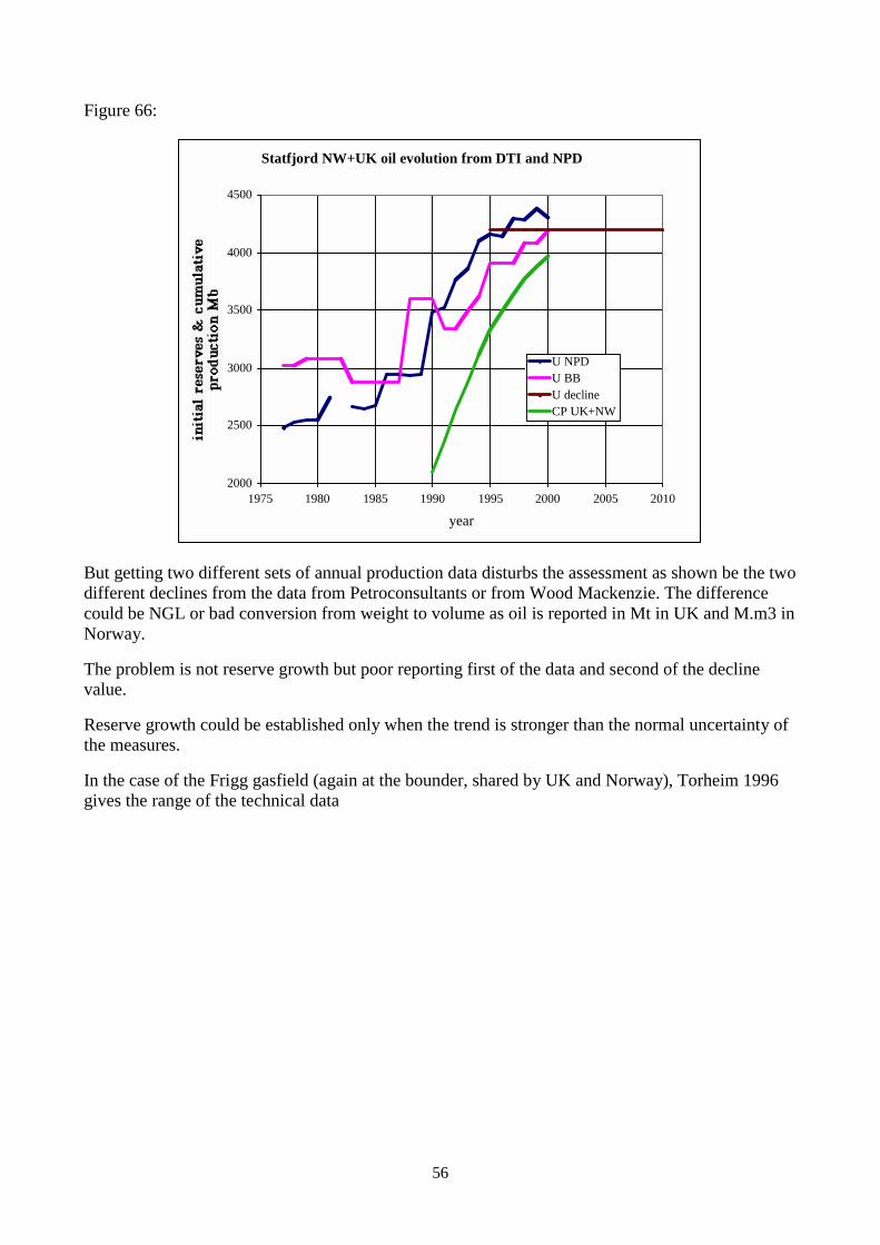
When the same field is shared by two countries as Statjford oilfield, the estimates from the twonational agencies differ much more than the reported growth from one source. In 1998 the ultimatewas estimated at 4386 Mb (4 significant digits what accuracy!) by NPD and 4088 Mb by the BrownBook but in fact the decline estimate gives 4200 Mb since 1995.

56

Figure 66:

Statfjord NW+UK oil evolution from DTI and NPD

2000

2500

3000

3500

4000

4500

1975 1980 1985 1990 1995 2000 2005 2010

year

U NPDU BBU declineCP UK+NW

But getting two different sets of annual production data disturbs the assessment as shown be the twodifferent declines from the data from Petroconsultants or from Wood Mackenzie. The differencecould be NGL or bad conversion from weight to volume as oil is reported in Mt in UK and M.m3 inNorway.

The problem is not reserve growth but poor reporting first of the data and second of the declinevalue.

Reserve growth could be established only when the trend is stronger than the normal uncertainty ofthe measures.

In the case of the Frigg gasfield (again at the bounder, shared by UK and Norway), Torheim 1996gives the range of the technical data

57

Figure 67:

Frigg: evolution of OGIP, RF and reserves withtime and more works

0

50

100

150

200

250

300

1970 1975 1980 1985 1990 1995 2000

year

in place

technicalreservesRF

reservesBBreservesNPD

In 1975 the reserve range was between 165 and 230 G.m3. The highest value was officially reportedin order to get the highest DCQ (daily contractual quantity) giving the highest profit. The gas inplace varies as the reserves as the RF stays around 75%, except for one study.

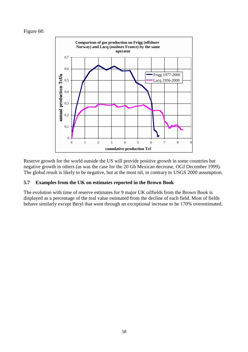
The comparison of the depletion of Frigg offshore UK-NW and Lacq onshore France is striking asthey were depleted by the same operator (Elf) but Frigg in 20 years (plateau over 5.5 Tcf/a from1980 to 1985) and Lacq in 50 years (plateau over 0.2 Tcf/a from 1961 to 1985). However becauseof high H2S in Lacq gas the capacity of the plant to extract the sulphur was a constraint for thisfield

58

Figure 68:

Comparison of gas production on Frigg (offshoreNorway) and Lacq (onshore France) by the same

operator

0

0,1

0,2

0,3

0,4

0,5

0,6

0,7

0 1 2 3 4 5 6 7 8 9

cumulative production Tcf

Frigg 1977-2000Lacq 1956-2000

Reserve growth for the world outside the US will provide positive growth in some countries butnegative growth in others (as was the case for the 20 Gb Mexican decrease, OGJ December 1999).The global result is likely to be negative, but at the most nil, in contrary to USGS 2000 assumption.

5.7 Examples from the UK on estimates reported in the Brown Book

The evolution with time of reserve estimates for 9 major UK oilfields from the Brown Book isdisplayed as a percentage of the real value estimated from the decline of each field. Most of fieldsbehave similarly except Beryl that went through an exceptional increase to be 170% overestimated.

59

Figure 69:

UK main oilfields ultimate from the Brown Book inpercentage of the ultimate estimate from decline

50

60

70

80

90

100

110

120

130

140

150

160

1975 1980 1985 1990 1995 2000

year

BerylBrentClaymoreFortiesFulmarMagnusNinianPiperThistleaverage

It shows that the average went into a growth from 1980 to 1993 but it was already overestimatedsince 1993 and in 2000 it is still 2% overestimated. The reserve growth started when over 50% ofthe ultimate was produced and flattened when 75% was produced. Now 90% has been produced.

Figure 70:

UK 9 largest oilfields: ultimate from the Brown Book &cumulative production in percentage of the ultimate estimate

from decline

30

40

50

60

70

80

90

100

110

1980 1985 1990 1995 2000

year

average ultimateaverage cumulative production

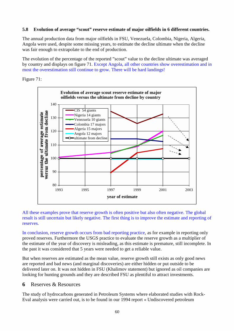
60

5.8 Evolution of average “scout” reserve estimate of major oilfields in 6 different countries.

The annual production data from major oilfields in FSU, Venezuela, Colombia, Nigeria, Algeria,Angola were used, despite some missing years, to estimate the decline ultimate when the declinewas fair enough to extrapolate to the end of production.

The evolution of the percentage of the reported ”scout” value to the decline ultimate was averagedby country and displays on figure 71. Except Angola, all other countries show overestimation and inmost the overestimation still continue to grow. There will be hard landings!

Figure 71:

Evolution of average scout reserve estimate of majoroilfields versus the ultimate from decline by country

80

90

100

110

120

130

140

1993 1995 1997 1999 2001 2003

year of estimate

CIS 54 giantsNigeria 14 giantsVenezuela 10 giantsColombia 17 majorsAlgeria 15 majorsAngola 12 majorsultimate from decline

All these examples prove that reserve growth is often positive but also often negative. The globalresult is still uncertain but likely negative. The first thing is to improve the estimate and reporting ofreserves.

In conclusion, reserve growth occurs from bad reporting practice, as for example in reporting onlyproved reserves. Furthermore the USGS practice to evaluate the reserve growth as a multiplier ofthe estimate of the year of discovery is misleading, as this estimate is premature, still incomplete. Inthe past it was considered that 5 years were needed to get a reliable value.

But when reserves are estimated as the mean value, reserve growth still exists as only good newsare reported and bad news (and marginal discoveries) are either hidden or put outside to bedelivered later on. It was not hidden in FSU (Khalimov statement) but ignored as oil companies arelooking for hunting grounds and they are described FSU as plentiful to attract investments.

6 Reserves & Resources

The study of hydrocarbons generated in Petroleum Systems where elaborated studies with Rock-Eval analysis were carried out, is to be found in our 1994 report « Undiscovered petroleum

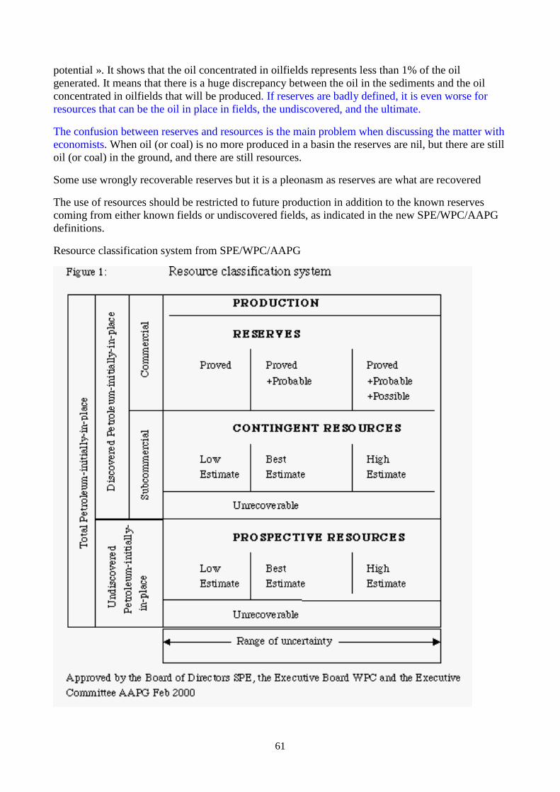
61

potential ». It shows that the oil concentrated in oilfields represents less than 1% of the oilgenerated. It means that there is a huge discrepancy between the oil in the sediments and the oilconcentrated in oilfields that will be produced. If reserves are badly defined, it is even worse forresources that can be the oil in place in fields, the undiscovered, and the ultimate.

The confusion between reserves and resources is the main problem when discussing the matter witheconomists. When oil (or coal) is no more produced in a basin the reserves are nil, but there are stilloil (or coal) in the ground, and there are still resources.

Some use wrongly recoverable reserves but it is a pleonasm as reserves are what are recovered

The use of resources should be restricted to future production in addition to the known reservescoming from either known fields or undiscovered fields, as indicated in the new SPE/WPC/AAPGdefinitions.

Resource classification system from SPE/WPC/AAPG

62

About 90% of reserve additions are revisions of past estimates because probable reserves areignored. Good practices should lead to statistically neutral revisions. In the rest of the world, suchas the North Sea, reserves are reported as proven + probable. Development of a large offshoreplatform only occurs after several appraisal wells have determined that the proven + probablereserves are sufficient to justify a profitable development. Proven reserves are inadequate for suchan analysis. A. Martinez (head of the SPE/WPC/AAPG reserve task force) has approached the SECto accept proved + probable instead of proved reserves. In Russia, use of reliable reserve data willlead to negative reserve growth from 3P to 2P.

7 Ultimates

World ultimates have been assessed by aggregating regional studies, in the past using the volume ofsedimentary basins and analogy with other producing basins, later extrapolating creaming curves orsizes distribution of mature basins. It was done by country, or by tectonic basins, or lately bygenetic basins (Petroleum System). It was mainly done by the major companies, but they stoppedwhen they reduced staff and when the results started to look sad. Now it is left to governmentalagencies (as the USGS) or contractors (as Robertson) or to retired oil geologists concerned aboutthe future of their grandchildren.

7.1 Retired oil geologists group

Our ultimate estimate involves more than seven years of study by four retired explorationgeologists: Alain Perrodon, who was the first to introduce the term Petroleum System, GerardDemaison, who quantified generation of a Petroleum System, Colin Campbell and myself.

We are also in very close contact with two famous US retired geologists: Walter Youngquist(Geodestinies 1996) and Buzz Ivanhoe (Hubbert Centre at the Colorado School of Mines).

The four reports totalling 1250 pages from 1994 to 1998 are:

-Laherrère, J.H. A.Perrodon, and G.Demaison 1994 " Undiscovered Petroleum Potential";Petroconsultants Report 383p March

-Laherrère J.H., A.Perrodon, and C.J.Campbell 1996 "The world's gas potential" PetroconsultantsReport July, 200p, CD-ROM

-C.J.Campbell C.J.& J Laherrère 1995."The world's oil supply -1930-2050", PetroconsultantsReport 650p, CD-ROM

-Perrodon A., J.H. Laherrère and C.J.Campbell 1998 "The world's non-conventional oil and gas";Petroleum Economist March report 113p

Our ultimate is as follows:

Perrodon et al 1998 mini mean maxiConventional oil 1 700 1 800 2 200Conventional gas liquids 200 250 400Non-conventional liquids 300 700 1 500Ultimate liquids Gb 2 300 2 750 4 000

Conventional gas 8 500 10 000 13 000Non-conventional gas 1 000 2 500 8 000Ultimate gas Tcf 10 000 12 500 20 000

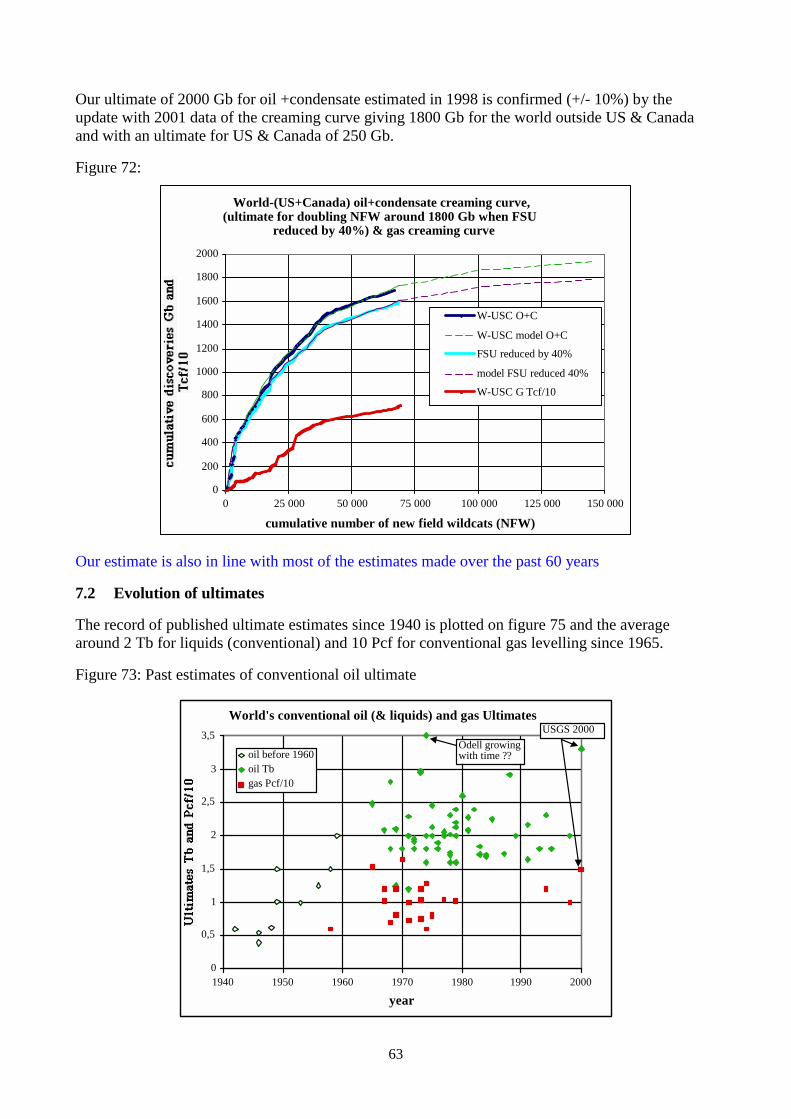
63

Our ultimate of 2000 Gb for oil +condensate estimated in 1998 is confirmed (+/- 10%) by theupdate with 2001 data of the creaming curve giving 1800 Gb for the world outside US & Canadaand with an ultimate for US & Canada of 250 Gb.

Figure 72:

World-(US+Canada) oil+condensate creaming curve,(ultimate for doubling NFW around 1800 Gb when FSU

reduced by 40%) & gas creaming curve

0

200

400

600

800

1000

1200

1400

1600

1800

2000

0 25 000 50 000 75 000 100 000 125 000 150 000

cumulative number of new field wildcats (NFW)

W-USC O+C

W-USC model O+C

FSU reduced by 40%

model FSU reduced 40%

W-USC G Tcf/10

Our estimate is also in line with most of the estimates made over the past 60 years

7.2 Evolution of ultimates

The record of published ultimate estimates since 1940 is plotted on figure 75 and the averagearound 2 Tb for liquids (conventional) and 10 Pcf for conventional gas levelling since 1965.

Figure 73: Past estimates of conventional oil ultimate

World's conventional oil (& liquids) and gas Ultimates

0

0,5

1

1,5

2

2,5

3

3,5

1940 1950 1960 1970 1980 1990 2000

year

oil before 1960oil Tbgas Pcf/10

Odell growingwith time ??

USGS 2000

64

Relying on the evolution of heterogeneous values to get the ultimate of ultimate (Odell & Rosing)1974) has no geological meaning and is little more than a mathematical game! Let us return to thebasic data and to the geologists who have carried out the assessments in detail.

P-R Bauquis (Journee de l’Energie Paris Mai 18, 2001): “There is practically no increase in theestimate of conventional oil ultimate from 1973 to 2000.”

7.3 USGS world assessment 2000

This study was a good project to define first all the Petroleum Systems of the world with the help ofthe major oil companies and to draw good maps, but the results were poor because the oilcompanies did not participate in the assessment, preferring to keep their knowledge and ideasconfidential since they were competing with each other for the prime areas. It was left to a singleUSGS geologist to assess each individual basin (in the past it was done with Delphi inquiriesinvolving many geologists). It was done without the benefit of seismic coverage and well data.Most of the estimates were made by academic geologists with little oil exploration practice. Thedatabase for reserves by field was 1995 & 1996 was out of date for a 2000 assessment and it wasalso inconsistent, with Proved reserves being used for the US and Canada (P) and Proved &Probable reserves (2P) being used the rest of the world.

The USGS study is considered by some to be a geological rather than a statistical study. It relies onmany Monte Carlo simulations based on poor estimates of undiscovered sizes and numbers.Furthermore the past discovery data is old data (1996) when better-updated data exist.

The only parameters asked to the USGS geologist were to give:

http://greenwood.cr.usgs.gov/pub/bulletins/b2165/B2165.pdf

-Characteristics of the assessment unit:

-the minimum size

-number of discovered fields exceeding the minimum size

-median size of discovered oil and gas fields

-probability of geological charge, rocks and timing plus the adequate location for activities

-Undiscovered oil and gas Fields

-number of undiscovered fields with minimum, median and maximum

-sizes of undiscovered fields with minimum, median and maximum.

A second page asks for the gas/oil ratio, the density, the sulphur content and the drilling depth anddepth of water.

That was all that the geologist has to supply. From this sheet of papers, a lot of time and moneywere spent running Monte Carlo simulations. Out of the 32 000 pages of this report, apart thegeological maps, the main hypothesis on the 105 ranked assessment units for undiscovered oil wasonly 105 pages. The five largest undiscovered provinces are given as:

Province undiscovered oil

Mesopotamian Foredeep Basin 61 Gb

West Siberian Basin 55 Gb

65

East Greenland Rift Basins 47 Gb

Zagros Fold Belt 45 Gb

Niger Delta 40 Gb

7.3.1 East Greenland

The East Greenland is undrilled but non-exclusive seismic surveys are available (but veryexpensive) as shown in the figure 74. The USGS did not acquire this seismic data, but assume thatit will show all the necessary components.

Figure 74:

The USGS assessment gives a 100% geological probability of oil occurrence, but only 70% foraccess (it is covered most of the time with ice!)

The description of the Petroleum System is reduced to the following guess:

<<USGS PROVINCES: Northeast Greenland Rift Basins (5200) GEOLOGIST: M.E. Henry

TOTAL PETROLEUM SYSTEM: Permian/Upper Jurassic Composite (520001)

ASSESSMENT UNIT: Northeast Greenland Shelf Rift Systems (52000101)

DESCRIPTION: This assessment unit includes the continental margin off eastern and northeasternGreenland and is almost entirely offshore. The eastern boundary extends to the approximateposition of the boundary between continental and oceanic crust, the northern boundary separatesthis province from the Wandell Sea Basin, the southern boundary is placed near lat. 70 N. and thewestern boundary is drawn to include the nearshore deep sub-basins on the shelf that have beeninterpreted from geophysical data.

SOURCE ROCKS: The principal source rock for this unit is expected, primarily by analogy withthe Norwegian shelf and the Viking Graben of the North Sea, to be Late Jurassic shales of the

66

Hareelv Formation. Other potential source rocks probably exist in the unit and include, in order ofexpected importance, the Upper Permian Ravenfjeld Formation, Upper Carboniferous lacustrineshales, the Lower Jurassic Kap Stewart Formation, and other Devonian and Triassic beds.

MATURATION: Little published data exits in the offshore area regarding thermal maturity of theselikely sources. Considering the probable depths of the source rocks in the numerous sub-basins thatexist on the shelf, which are as deep as 10 km, thermal maturity for petroleum generation must havebeen reached at least locally in these depressions.

MIGRATION: Because of the nature of structural deformation in this unit lateral migration may berather limited but vertical migration could have been important.

RESERVOIR ROCKS: Principal reservoir rocks are expected to be sandstones of the MiddleJurassic Vardekløft and Olympen Formations. Other important reservoir units include carbonatebuild-ups in the Upper Permian and sands of the Lower Jurassic Kap Stewart and Neill KlintnerFormations.

TRAPS AND SEALS: The system of fault blocks, rotated generally landward, lead to theexpectation that major traps are likely to be found in the uplifted side of the blocks and that faultingwill be important in trap formation. Overlying shales will form top seals for many traps.

REFERENCES: -Christiansen, F.G., Dam, G., Piasecki, S., and Stemmerick, L., 1992, A review ofUpper Paleozoic and Mesozoic source rocks from onshore East Greenland. -Larsen, H.C., 1990,The east Greenland shelf, -Price, S.P., and Whitham, A.G., 1997, Exhumed hydrocarbon traps ineast Greenland–analogs for the Lower-Middle Jurassic play of northwest Europe<<

It is obvious that the USGS has no access to the seismics and that they speculate that traps will bethere. Their references (1990, 1992 & 1997) are not up to date!

The distribution given by Henry is for oil: for the number, 1-250-500 undiscovered oilfields, for thesize, 20-85-12000 Mb, for the gravity: 15-40-55 °API. For gas, the distribution is 1-50-100 innumber and 0.12-0.5-20 Tcf in size.

These simple numbers with a huge range show that they come from nowhere, being just pureguesses and wishful thinking!

From this ungeological assessment, Monte Carlo simulation gives a beautiful distribution.

No scientific credence can be given to work of this sort.

67

Figure 75:

Comparing this assumed oil size distribution on East Greenland to the North Sea (Viking grabens)on a fractal display, shows that the assumed East Greenland is richer than the real North Sea.

Figure 76:

There are less than 40 oilfields larger than 100 Mb in the Viking grabens, whereas East Greenlandis assumed to contain about 100 oilfields over 100 Mb (and the probability is supposed to be100%!)

68

7.3.2 Lower 48 Reserve growth used worldwide?

Another dream from the USGS 2000 is about reserve growth. It is derived from the bad US practiceof reporting, to comply with the SEC rules, only proved reserves when the rest of the world reportsproven+probable. Ignoring probable reserves leads to a huge upward revision and 90% of theannual addition come from revisions of old discoveries.

Chuck Masters, the previous director of the studies, had a sound understanding of the position. andhis USGS evaluation did not use Proved Reserves but Inferred Reserves (he corrected them toinclude Probable) and he pointed that the reserve growth is likely to be negligible in comparison ofthe large number of reported discoveries which are marginal and maybe never developed.

In the chapter of reserve growth in the USGS 2000 study; the authors Schmoker and Klett wrote:

<<<Therefore, patterns of reserve growth for the world as a whole are poorly understood, and theproblem of quantitatively estimating world potential reserve growth is formidable. For most areasoutside the United States and Canada, however, Attanasi and Root (1993) and Root and Attanasi(1993) concluded that successive field-size estimates were not sufficiently reliable and consistent todevelop world-level reserve-growth functions. At the time of the World Petroleum Assessment2000, available world field-size estimates still appear to be inadequate—in terms of completeness,quality, and internal consistency—to construct a credible world reserve-growth function. . That is tosay, the preferred approach outlined above to developing a world reserve-growth function cannot beimplemented because of data limitations. Given this conclusion, three reserve-growth options wereconsidered for the World Petroleum Assessment 2000:

-1. Defer the forecasting of world potential reserve growth to some future assessment.

-2. Forecast potential reserve growth for those relatively few areas of the world where field-sizeestimates are adequate to establish local reserve-growth functions.

-3. Forecast potential reserve growth at the world level by using an analog model that incorporatesthe reserve-growth experience of the United States. The third option is the one that has beenpursued, on the reasoning that, although the resulting preliminary forecast of world potential reservegrowth carries much uncertainty, a greater error would be to not consider world-level reservegrowth at all.

There are also several reasons why a reserve-growth function based on the Lower 48 states couldoverestimate world potential reserve growth:

-Engineering criteria for reporting reserves of world oil and gas fields might, in general, be lessrestrictive than those for the United States, tending to increase known reserves and decrease thepotential for reserve growth.

-Reported reserves might be deliberately overstated in some countries, reducing the potential forfuture reserve growth.

-Large world oil and gas fields might tend to have more substantial development than U.S. fieldsprior to release of initial field-size estimates, leading to more accurate initial reserves estimates andreducing the potential for future reserve growth. The balance that will ultimately emerge from theseand other influences upon world reserve growth relative to U.S. reserve growth is unclear.<<<

Despite admitting that they are unable to give a reserve growth for the world, they use the Lower 48for the rest of the world. This Lower 48 comes from the evolution of estimates made 50 years agoon onshore old fields at a time when seismic was not routine. And, even worse, they apply such a

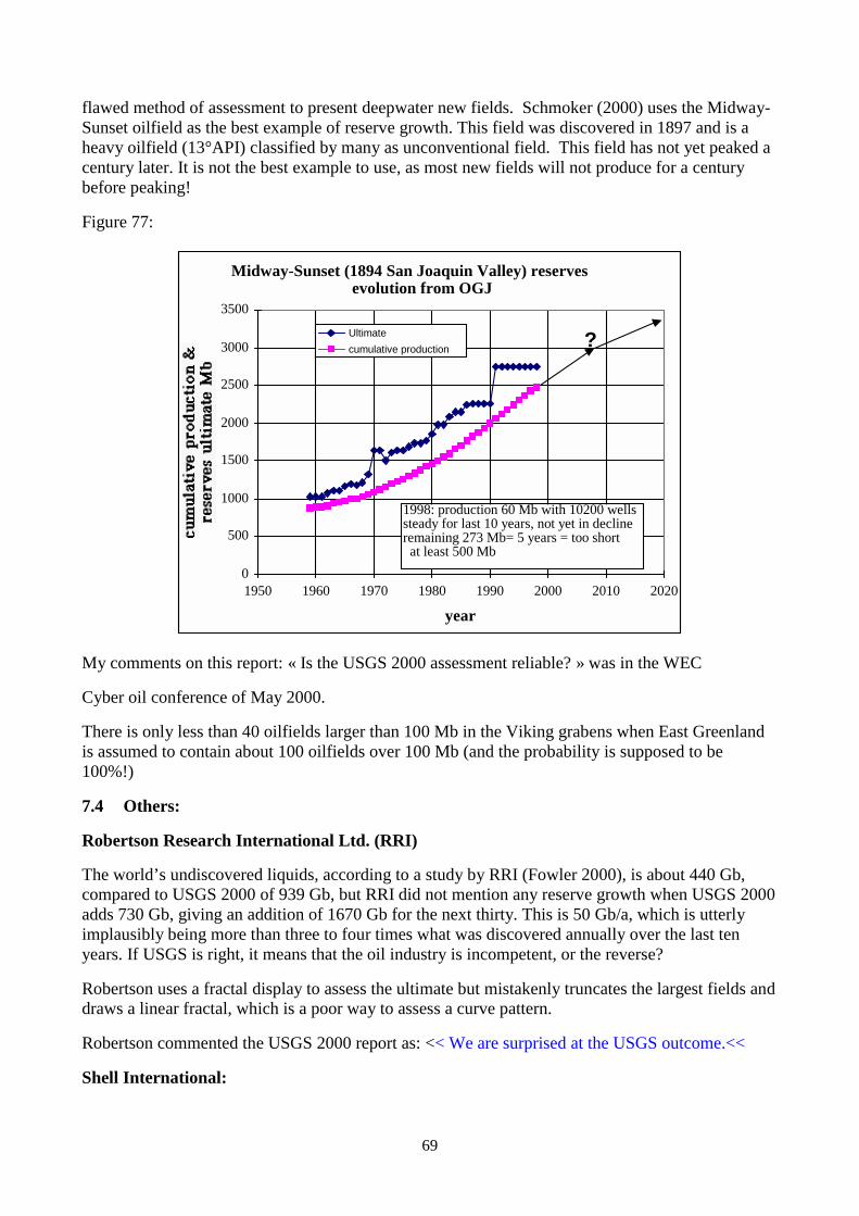
69

flawed method of assessment to present deepwater new fields. Schmoker (2000) uses the Midway-Sunset oilfield as the best example of reserve growth. This field was discovered in 1897 and is aheavy oilfield (13°API) classified by many as unconventional field. This field has not yet peaked acentury later. It is not the best example to use, as most new fields will not produce for a centurybefore peaking!

Figure 77:

Midway-Sunset (1894 San Joaquin Valley) reservesevolution from OGJ

0

500

1000

1500

2000

2500

3000

3500

1950 1960 1970 1980 1990 2000 2010 2020

year

Ultimate

cumulative production ?

1998: production 60 Mb with 10200 wellssteady for last 10 years, not yet in declineremaining 273 Mb= 5 years = too shortat least 500 Mb

My comments on this report: « Is the USGS 2000 assessment reliable? » was in the WEC

Cyber oil conference of May 2000.

There is only less than 40 oilfields larger than 100 Mb in the Viking grabens when East Greenlandis assumed to contain about 100 oilfields over 100 Mb (and the probability is supposed to be100%!)

7.4 Others:

Robertson Research International Ltd. (RRI)

The world’s undiscovered liquids, according to a study by RRI (Fowler 2000), is about 440 Gb,compared to USGS 2000 of 939 Gb, but RRI did not mention any reserve growth when USGS 2000adds 730 Gb, giving an addition of 1670 Gb for the next thirty. This is 50 Gb/a, which is utterlyimplausibly being more than three to four times what was discovered annually over the last tenyears. If USGS is right, it means that the oil industry is incompetent, or the reverse?

Robertson uses a fractal display to assess the ultimate but mistakenly truncates the largest fields anddraws a linear fractal, which is a poor way to assess a curve pattern.

Robertson commented the USGS 2000 report as: << We are surprised at the USGS outcome.<<

Shell International:

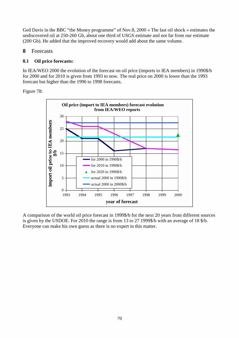
70

Ged Davis in the BBC “the Money programme” of Nov.8, 2000 « The last oil shock » estimates theundiscovered oil at 250-260 Gb, about one third of USGS estimate and not far from our estimate(200 Gb). He added that the improved recovery would add about the same volume.

8 Forecasts

8.1 Oil price forecasts:

In IEA/WEO 2000 the evolution of the forecast on oil price (imports to IEA members) in 1990$/bfor 2000 and for 2010 is given from 1993 to now. The real price on 2000 is lower than the 1993forecast but higher than the 1996 to 1998 forecasts.

Figure 78:

Oil price (import to IEA members) forecast evolutionfrom IEA/WEO reports

0

5

10

15

20

25

30

1993 1994 1995 1996 1997 1998 1999 2000

year of forecast

for 2000 in 1990$/b

for 2010 in 1990$/b

for 2020 in 1990$/b

actual 2000 in 1990$/b

actual 2000 in 2000$/b

A comparison of the world oil price forecast in 1999$/b for the next 20 years from different sourcesis given by the USDOE. For 2010 the range is from 13 to 27 1999$/b with an average of 18 $/b.Everyone can make his own guess as there is no expert in this matter.

71

Figure 79:

World oil price forecast from USDOE/AEO 2001

0

5

10

15

20

25

30

2000 2005 2010 2015 2020

forecasted year

DRI 2000

IEA 1998

PEL 2000

PIRA 2000

WEFA 2000

GRI 2000

DBAB 2000

NRCan1997AEO2001high priceAEO2001low priceAEO2001reference

The USDOE oil price forecast in 1999 was an increase from 15 $/b to 20 in 2005 and flat then until2020. In 2000 they corrected with a spike at 22$/b in 2000 (the price soared to 27$/b) returning tolow price in 2001. This year forecast is the 2000 spike will be back to 1999 forecast in 2002. Itseems that politics is more used than science and that there is a clear policy to keep the cheap oilforecast as the US way of life is based on cheap oil.

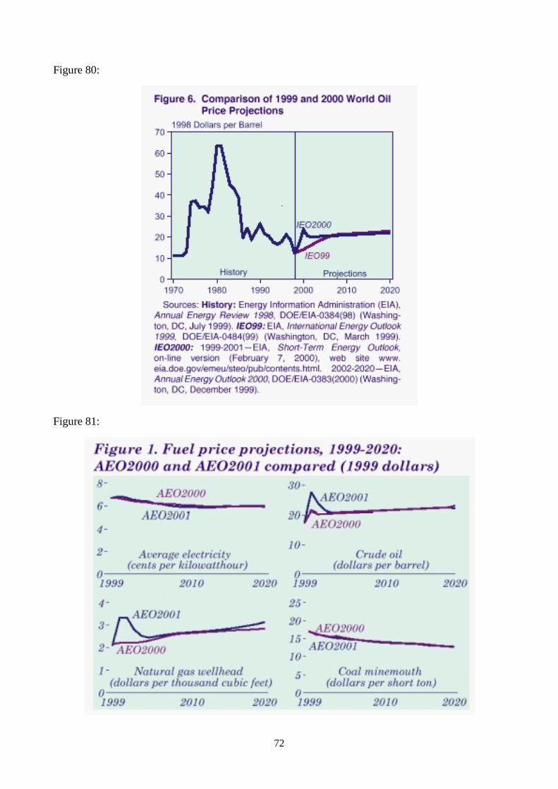
72

Figure 80:

Figure 81:

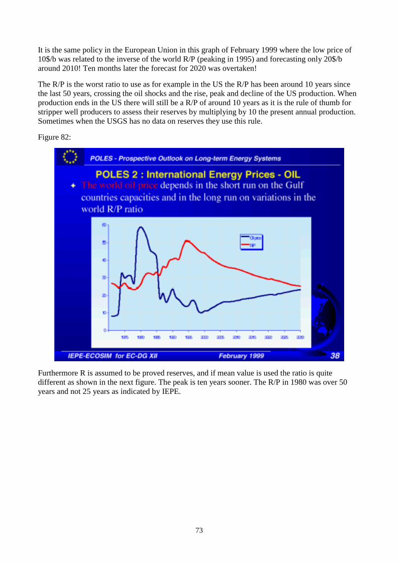
73

It is the same policy in the European Union in this graph of February 1999 where the low price of10$/b was related to the inverse of the world R/P (peaking in 1995) and forecasting only 20$/baround 2010! Ten months later the forecast for 2020 was overtaken!

The R/P is the worst ratio to use as for example in the US the R/P has been around 10 years sincethe last 50 years, crossing the oil shocks and the rise, peak and decline of the US production. Whenproduction ends in the US there will still be a R/P of around 10 years as it is the rule of thumb forstripper well producers to assess their reserves by multiplying by 10 the present annual production.Sometimes when the USGS has no data on reserves they use this rule.

Figure 82:

Furthermore R is assumed to be proved reserves, and if mean value is used the ratio is quitedifferent as shown in the next figure. The peak is ten years sooner. The R/P in 1980 was over 50years and not 25 years as indicated by IEPE.

74

Figure 83:

World R/P and US oil price $1999/b

0

10

20

30

40

50

60

1975 1980 1985 1990 1995 2000 2005 2010 2015 2020

year

R/P yearsforecast R/Pcrude oil $1999/b

?

While we have to wait many years to check if the forecast in volume is right, the impact on oil pricecomes much sooner. The consensus between official agencies is that in 2002 the oil price will belower than the goal of OPEC to get 25$/b. If the average in 2001 is over 25$/b it will indicate thatofficial forecasts are in trouble and if oil price stays at 25$/b in 2002 it will show the failure of theofficial forecasts. It will not be a surprise as the last oil shock (27$/b in 2000) was not forecasted byany agency or any economist. The only people in 1998 to speak about « The end of cheap oil » wasus (Scientific American March 1998) and Franco Bernabe, CEO ENI before retiring, Forbes June15, 1998 « Cheap oil: enjoy it when it lasts ») and Mike Bowlin CEO ARCO after having sold hiscompany to BP (« last days of the oil age » Feb.1999). Finally in mid 2000 Brown CEO of BPannounced that BP now means « Beyond Petroleum ».

9 Future production

9.1 Past forecast: Halbouty–Moody 1979:

Forecasting future production is difficult because world events may intervene changing the patterns,as happened in 1979.

Moody J.D. and Halbouty M., two well known oilmen, presented forecasts of oil production andpopulation at the World Petroleum Congress of 1979 ("World's ultimate reserves of crude oil"), asshown in Figure 16. They anticipated a production peak of 38 Gb/a in 1990 which was reasonablein resource terms, save that it failed to take into account the effects of the oil shocks of the 1970swhich cut demand, such that 1979 production was not surpassed for fifteen years. So far as theirpopulation forecast is concerned, they assume exponential growth, which has not been experiencedsince.

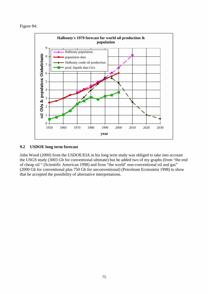
75

Figure 84:

Halbouty's 1979 forecast for world oil production &population

0

1

2

3

4

5

6

7

8

9

1950 1960 1970 1980 1990 2000 2010 2020 2030

year

Halbouty population.

population data

Halbouty crude oil production.

prod. liquids data Gt/a

9.2 USDOE long term forecast

John Wood (2000) from the USDOE/EIA in his long term study was obliged to take into accountthe USGS study (3003 Gb for conventional ultimate) but he added two of my graphs (from “the endof cheap oil “ (Scientific American 1998) and from “the world’ non-conventional oil and gas”(2000 Gb for conventional plus 750 Gb for unconventional) (Petroleum Economist 1998) to showthat he accepted the possibility of alternative interpretations.

76

Figure 85:

Figure 86:

77

Figure 87:

John Wood forecasts from the USGS ultimates a likely peak in 2016 at 35 Gb/a

Figure 88:

78

Les Magoon (USGS and author of some chapters of the USGS 2000) felt obliged to give a viewdifferent from that of the USGS 2000 and published a poster USGS open file 00-320 “Are werunning out of oil?” where he presents our graph from Scientific American.

9.3 IEA 1998 forecast

After an oil conference in Paris on Nov.11, 1997 at which the so-called pessimists (Campbell,Laherrere, Bentley) were asked to confront the so-called optimists (Aldelman, Lynch, Odell,Kenney), the IEA for the G8 Energy Ministers' Meeting in Moscow 31 March 1998 presented thefigure 9 of “World Energy Prospects to 2020” where the conventional oil peaks around 2013 andthe demand for 2020 is met only by producing “unidentified unconventional” oil (Bakhtiari 2001).It is a political way to say that it is very unlikely!

Figure 89:

This graph is given in WEO 1998, but the WEO 2000 is much more optimistic (no more peak forconventional) as the IEA long term analysis director has changed!

9.4 My forecast

Using my file of world’s (oil+condensate 2P) conventional discoveries and my estimate of 2000 Gband 10 000 Tcf of conventional ultimates, I drew the cumulative discoveries for oil+condensate andfor gas using a logistic model for the future and I applied the same model to the cumulativeproduction as shown in the following figure:

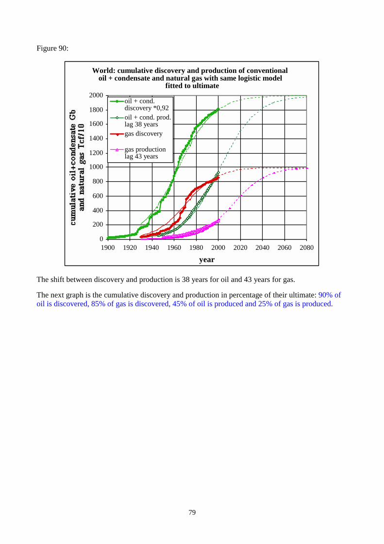
79

Figure 90:

World: cumulative discovery and production of conventionaloil + condensate and natural gas with same logistic model

fitted to ultimate

0

200

400

600

800

1000

1200

1400

1600

1800

2000

1900 1920 1940 1960 1980 2000 2020 2040 2060 2080

year

oil + cond.discovery *0,92oil + cond. prod.lag 38 yearsgas discovery

gas productionlag 43 years

The shift between discovery and production is 38 years for oil and 43 years for gas.

The next graph is the cumulative discovery and production in percentage of their ultimate: 90% ofoil is discovered, 85% of gas is discovered, 45% of oil is produced and 25% of gas is produced.

80

Figure 91:

World cumulative discovery and production of conventionaloil+condensate, gas in percentage of their ultimate (2000 Gb

& 10 000 Tcf)

0

10

20

30

40

50

60

70

80

90

100

1900 1920 1940 1960 1980 2000

year

gas discoverygas production lag 43 yearsoil + cond. discoveryoil + cond. prod. lag 38 years

9.5 Comparison different forecasts

The different forecasts for world’s oil production up to 2020 from USDOE/EIA IEO (InternationalEnergy Outlook), IEA WEO (World Energy Outlook), OPEC OWEM (OPEC’s World EnergyModel) and European Union are plotted with the past production from 1950 (usually only theforecast is shown without the past) with my own forecast as given above. The breakdown intoOPEC and Non-OPEC is given.

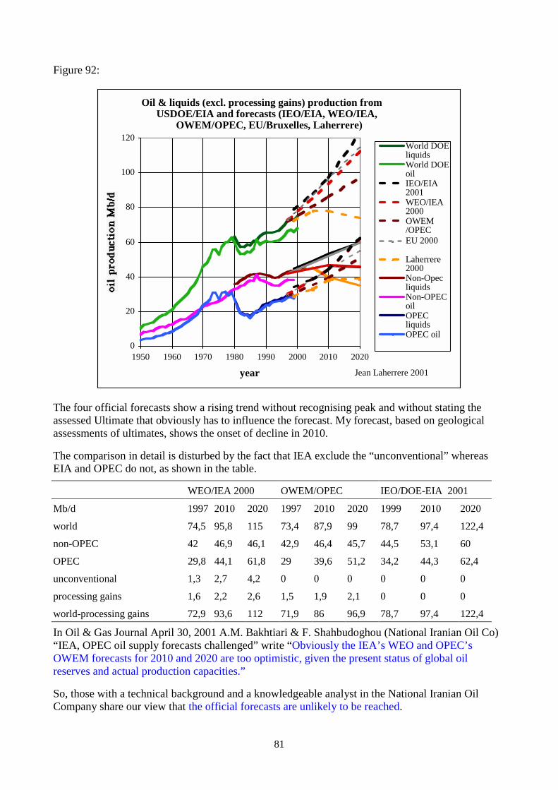
81

Figure 92:

Oil & liquids (excl. processing gains) production fromUSDOE/EIA and forecasts (IEO/EIA, WEO/IEA,

OWEM/OPEC, EU/Bruxelles, Laherrere)

0

20

40

60

80

100

120

1950 1960 1970 1980 1990 2000 2010 2020

year

World DOEliquidsWorld DOEoilIEO/EIA2001WEO/IEA2000OWEM/OPECEU 2000

Laherrere2000Non-OpecliquidsNon-OPECoilOPECliquidsOPEC oil

Jean Laherrere 2001

The four official forecasts show a rising trend without recognising peak and without stating theassessed Ultimate that obviously has to influence the forecast. My forecast, based on geologicalassessments of ultimates, shows the onset of decline in 2010.

The comparison in detail is disturbed by the fact that IEA exclude the “unconventional” whereasEIA and OPEC do not, as shown in the table.

WEO/IEA 2000 OWEM/OPEC IEO/DOE-EIA 2001

Mb/d 1997 2010 2020 1997 2010 2020 1999 2010 2020

world 74,5 95,8 115 73,4 87,9 99 78,7 97,4 122,4

non-OPEC 42 46,9 46,1 42,9 46,4 45,7 44,5 53,1 60

OPEC 29,8 44,1 61,8 29 39,6 51,2 34,2 44,3 62,4

unconventional 1,3 2,7 4,2 0 0 0 0 0 0

processing gains 1,6 2,2 2,6 1,5 1,9 2,1 0 0 0

world-processing gains 72,9 93,6 112 71,9 86 96,9 78,7 97,4 122,4

In Oil & Gas Journal April 30, 2001 A.M. Bakhtiari & F. Shahbudoghou (National Iranian Oil Co)“IEA, OPEC oil supply forecasts challenged” write “Obviously the IEA’s WEO and OPEC’sOWEM forecasts for 2010 and 2020 are too optimistic, given the present status of global oilreserves and actual production capacities.”

So, those with a technical background and a knowledgeable analyst in the National Iranian OilCompany share our view that the official forecasts are unlikely to be reached.

82

9.6 Global forecast oil &gas conventional and unconventional

In our 1998 World’s non-conventional oil and gas study, I plotted a forecast for world liquids(excluding refinery gains) together with detailed of modelling for conventional oil, unconventionaloil and gas liquids. The actual record over the last two years data confirms the curve. I also add thegross gas production (the dry production is about 85% of the gross). Mostly, only dry gasproduction is reported, whereas the remaining reserves are estimated in terms of gross volumes – afurther source of confusion.

The indicated peak for liquids (75 Mb/d in 2000) is before 2010 at 28 Gb/a (80 Mb/d)

The peak for gas (90 Tcf/a or 15 Gboe/a in 2000) is in 2030 at 135 Tcf/a or 22.5 Gboe.

Figure 93:

World liquids & gross gas future production fromultimates (conventional + non-conventional) 2750 Gb and

12 500 Tcf (Perrodon, Laherrere, Campbell 1998)

0

5

10

15

20

25

30

1925 1950 1975 2000 2025 2050 2075 2100 2125

year

past productionliquids

conventional oil

gas liquids

non-conventional oil

conventional + non-conventional liquids

past productiongross gas

conventional + non-conventional naturalgas 1 Gboe= 6Tcf

Jean Laherrere 2001

9.7 Global forecast per capita

The global above oil plus gas forecast is plotted in the next graph per capita, using the UnitedNations 1999 forecast with the low/medium fertility rate. The reference case (medium fertility ratetaken as 2.1 to obtain the replacement ratio that gives a steady population) is unrealistic. Everydecrease in fertility rate in developed countries did not stop at 2.1, but went down to 1.5 in average,even 1.1 for Spain and Italy. In this scenario, world population peaks in 2050 at less than 8 billion.

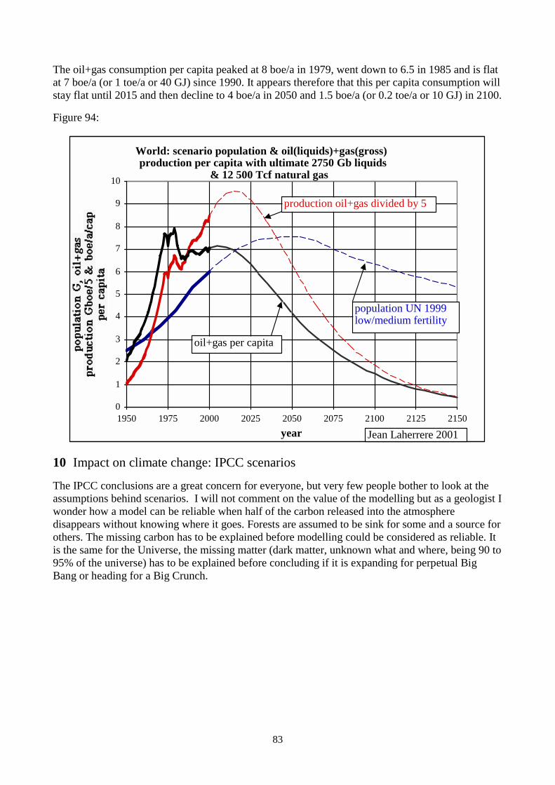
83

The oil+gas consumption per capita peaked at 8 boe/a in 1979, went down to 6.5 in 1985 and is flatat 7 boe/a (or 1 toe/a or 40 GJ) since 1990. It appears therefore that this per capita consumption willstay flat until 2015 and then decline to 4 boe/a in 2050 and 1.5 boe/a (or 0.2 toe/a or 10 GJ) in 2100.

Figure 94:

World: scenario population & oil(liquids)+gas(gross)production per capita with ultimate 2750 Gb liquids

& 12 500 Tcf natural gas

0

1

2

3

4

5

6

7

8

9

10

1950 1975 2000 2025 2050 2075 2100 2125 2150

year

population UN 1999low/medium fertility

oil+gas per capita

production oil+gas divided by 5

Jean Laherrere 2001

10 Impact on climate change: IPCC scenarios

The IPCC conclusions are a great concern for everyone, but very few people bother to look at theassumptions behind scenarios. I will not comment on the value of the modelling but as a geologist Iwonder how a model can be reliable when half of the carbon released into the atmospheredisappears without knowing where it goes. Forests are assumed to be sink for some and a source forothers. The missing carbon has to be explained before modelling could be considered as reliable. Itis the same for the Universe, the missing matter (dark matter, unknown what and where, being 90 to95% of the universe) has to be explained before concluding if it is expanding for perpetual BigBang or heading for a Big Crunch.

84

The assumptions of the IPCC 2000 are as follows, compared to the World Energy Assessment(United Nations and World Energy Council)

IPCC 2000 Emission scenarios World Energy AssessmentA1FI A1B A1T A2 B1 B2 growth A growth B growth C

high middle ecologicallypopulation G1990 5,3 5,3 5,3 5,3 5,3 5,3 5,3 5,3 5,32020 7,6 7,5 7,6 8,2 7,6 7,62050 8,7 8,7 8,7 11,3 8,7 9,3 10,1 10,1 10,12100 7,1 7,1 7 15,1 7 10,4 11,7 11,7 11,7per capita per yearprimary energy GJ1990 65 65 65 65 65 65 72 72 722020 90 90 80 70 80 702050 160 150 140 90 90 90 103 83 602100 290 310 290 110 70 130 159 125 75GDP k$19901990 4 4 4 4 4 4 4 4 42020 7 7 8 5 7 72050 20 20 20 7 15 10 10 7 72100 75 75 80 15 50 20 26 17 19

CO2 fossil fuels tC1990 1,1 1,1 1,1 1,1 1,1 1,1 1,1 1,1 1,12020 1,5 1,6 1,3 1,3 1,3 1,22050 2,7 1,8 1,4 1,5 1,3 1,2 1,2 1,0 0,52100 4,3 1,8 0,7 1,9 0,7 1,3 1,1 0,9 0,2CO2 concentration ppm1990 350 350 350 350 350 350 358 358 3582020 410 415 410 410 410 4052050 565 530 500 530 480 470 460-510 470 4602100 960 705 570 840 540 610 530-730 590 460

10.1 Population

Whereas IPCC 1995 was high on population, IPCC 2000 is much lower. Most assumptions are 7billion in 2100 (but one at 15) compared to 12 billion for WEA and 6.5 in the UN low/mediumfertility.

10.2 Primary energy

The primary energy per capita being 65 GJ in 2000 is assumed to be around 300 GJ in case A1 andaround 100 BJ in the other scenarios (about the same order for the WEA). In our scenario theenergy from oil and gas will be in 2100 around 10 GJ; it means that oil and gas will represents only10% of the energy consumption. It is unlikely.

10.3 Primary energy for oil and for gas

Out of the 40 scenarios (http://www.grida.no/climate/ipcc/emission/data/allscen.xls) giving thedetail of primary energy for oil on the following graph, most of them are out of range with my

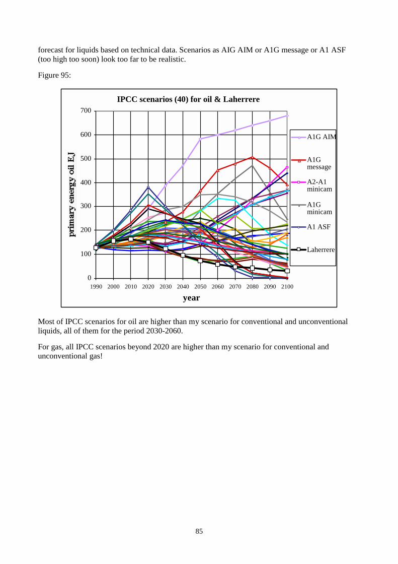
85

forecast for liquids based on technical data. Scenarios as AIG AIM or A1G message or A1 ASF(too high too soon) look too far to be realistic.

Figure 95:

IPCC scenarios (40) for oil & Laherrere

0

100

200

300

400

500

600

700

1990 2000 2010 2020 2030 2040 2050 2060 2070 2080 2090 2100

year

A1G AIM

A1Gmessage

A2-A1minicam

A1Gminicam

A1 ASF

Laherrere

Most of IPCC scenarios for oil are higher than my scenario for conventional and unconventionalliquids, all of them for the period 2030-2060.

For gas, all IPCC scenarios beyond 2020 are higher than my scenario for conventional andunconventional gas!

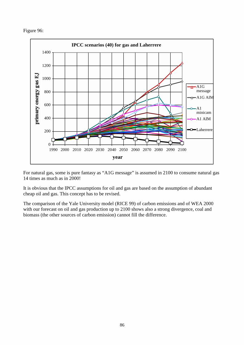
86

Figure 96:

IPCC scenarios (40) for gas and Laherrere

0

200

400

600

800

1000

1200

1400

1990 2000 2010 2020 2030 2040 2050 2060 2070 2080 2090 2100

year

A1Gmessage

A1G AIM

A1minicam

A1 AIM

Laherrere

For natural gas, some is pure fantasy as “A1G message” is assumed in 2100 to consume natural gas14 times as much as in 2000!

It is obvious that the IPCC assumptions for oil and gas are based on the assumption of abundantcheap oil and gas. This concept has to be revised.

The comparison of the Yale University model (RICE 99) of carbon emissions and of WEA 2000with our forecast on oil and gas production up to 2100 shows also a strong divergence, coal andbiomass (the other sources of carbon emission) cannot fill the difference.

87

Figure 97:

Comparison forecasts Rice 99 & WEA2000carbon emission and our oil and gas production

0

20

40

60

80

100

120

140

160

180

1980 2000 2020 2040 2060 2080 2100 2120 2140 2160 2180 2200

year

Laherrere oil EJ

Laherrere gas EJ

oil+gas EJ*0,32

Rice 99 emissionGtC/a *10WEA emissionGtC/a*10

The WEA consumption for the period 1990-2100 in PJ for their 3 cases is compared to our forecast:

PJ=10E15 J WEA WEA WEA

1990-2100 Laherrere A high growth B middle growth C ecolog. growth

oil 9,8 27,6-15,7 15,3 10,9

gas 9,3 18,4-28,7 15,8 12,2-12,9

WEA future consumption for the middle case of oil and gas for the next century is 50% above ourforecast.

10.4 GDP

In 1990 the world GPD per capita was 4 k1990$, in 2100 the assumption is 75 k1990$ for A1 andabout 20 for the other scenarios (as for WEA). It is claimed that “oil” is replaced by “information”.The importance of oil is denied in front of the emergence of Internet or the huge increase of GPD.Anthony Blair, Prime Minister of the United Kingdom at the World Economic Forum AnnualMeeting 2000 Friday, January 28, 2000, Davos, Switzerland: "Twenty years on from the oil shockof the 70s, most economists would agree that oil is no longer the most important commodity in theworld economy. Now, that commodity is information” Eight months later... Blair sends for thetroops, saying: "Troops were put on standby last night to intervene in the deepening fuel crisis as

88

the health service went on emergency alert, supermarkets began rationing food and schools andbusinesses closed."

In the following graph from 1949 the US relative increase to 2000 is: population 180%, energyconsumption 300% and GDP almost 600%.

Figure 98:

US energy parameters in percentage of 1949 value

0

100

200

300

400

500

600

1950 1960 1970 1980 1990 2000

year

Total EnergyConsumption

Gross DomesticProduct Value

Total EnergyConsumptionper Capita

Total ResidentPopulation

Total EnergyConsumed byGDP

It is difficult to see such increase in GPD with little correlation with population and energy since1973. The US GPD is manipulated using inflation and “hedonic” factor. When computer orsoftware doubles in memory or speed, the productivity is assumed to double and the realinvestments are doubled too through the “hedonic” factor to get into GPD. There are protests inGermany and UK about US practice: Richebacher (2000) « Had the German statisticians applied theU.S. methods for deflating IT equipment, according to the Bundesbank, real IT investment inGermany in 1998 would have been DM 64 billion, that is, twice as high as reported. In 1999, thedifference would have risen to 170%. »

The China GDP is known to be overestimated and the FSU GDP underestimated as a good part oftrade has been barter since the FSU break-up.

It is why energetic intensity has to be treated with caution. I prefer not to use it.

10.5 Heating and cooling days: interesting parameter

In the energy parameters recorded with care in the US are the heating and cooling days. They showa low around 1970, as it is well known that the global temperature went down from 1940 to 1970.In 1970 the concern was about global cooling and not global warming as it is now.

89

Figure 99:

US heating & cooling degree-days

1000

1100

1200

1300

1400

1500

1600

1700

1800

1900

2000

1940 1950 1960 1970 1980 1990 2000

year

6000 -Heating Degree-Days

Cooling Degree-Days

Deutsche Bank shows a longer trend from 1930 to 2000 on heating days with three cycles or a cycleof about 23 years (or one solar cycle as the solar period is 11 years but with change polarity). It is inagreement with the Svensmark theory of the impact of cosmic rays from the sun cycles on clouds.Clouds are the most important factor in temperature, more than CO2.

90

Figure 100:

Conclusions:

The consuming society thinks it needs growth to be happy. It is understandable therefore thateverything is presented in order to give hopes for growth.

The goal of the oil companies is to make profit. They have no obligation to publish data, beyondthat legally required of them. They prefer to keep information confidential, partly because it wouldbe useful to competitor, and they prefer to publish what improves their image.

Government agencies follow the policy of every government that promises that tomorrow will bebetter than today and relies on growth to solve all future problems.

Future oil and gas demand is overestimated because the estimates assume cheap prices and largeresources.

There are two or three different and parallel worlds involved in estimating oil reserves. They aresometimes described as pessimists and optimists, but they are neither. One world comprises oilexecutives who gained the freedom to speak when retired, and had experience and access toconfidential technical data. The other world comprises « academic writers » and/or economists, whotalk about future miracles of technology (but refusing to listen to technicians) and rely on publisheddata which are mainly political. There are also “theoretical writers” who deal only with theories andwishful thinking. They present ideas as facts, and reject facts as confusing.

The oil industry follows archaic and poor practices in reporting data for both production andreserves because confidentiality, conservatism and fear of the impact on the stock market.

Forecasts cannot be more unreliable than the underlying basic data.

91

However data on past discoveries and production shows that oil and gas liquids will peak before2010, and that natural gas will peak around 2030.

The IPCC assumptions on energy up to 2100 are accordingly unrealistic being based on cheap andabundant oil and gas.

Good estimates of oil reserves need good data, which are almost impossible to obtain even whererecords are in the public domain as in the Federal Gulf of Mexico where the USDOI/MMS datashows unpardonable mistakes.

It is important as a matter of urgency that the oil industry and the governmental agencies start torealise that the main priority now is to improve the world database. Indeed, that was the goal of arecent meeting in Bangkok (April 2-3) between six organisations and 20 producing and consumingcountries.

The ideal is to find an organisation, which is apolitical, in which consumers, and producers cantrust. I do not see any organisation that complies with the necessary qualities. IIASA could onepossibility. IIASA has to show that it can do it.

References:

-Attanasi E.D. & Root D.H. 1994 "The enigma of oil and gas field growth" AAPG 78/3 March, table 1

-Bakhtiari A.M.S., Shahbudaghlou F. 2001 « IEA, OPEC oil supply forecasts challenged » OGJ April 30,

-Bauquis P-R. 2001 “Quelles energies pour un developpement durable” Journees de l’energie au Palais de ladecouverte 18 Mai

-Bernabe F. 1998 « Cheap oil: enjoy it while it lasts » Forbes June 15http://www.forbes.com/asp/redir.asp?/forbes/98/0615/6112084a.htm

-Blair A. 2000 “Special message" World Economic Forum Annual Meeting 2000 Davos, Switzerlandhttp://www.asiamedia.ucla.edu/Davos2000/Speeches/Blair.htm

-Bowlin M. 1999 « last days of oil age have begun » ARCO press release Feb.9http://www.arco.com/Corporate/news/p020999.htm

-Campbell C.J, Laherrere J.H. 1998 "The end of cheap oil" Scientific American March p80-85

-Gochenour D.T. 1997 “Practical difficulties of valuing Russian oil reserves” SPE 37958

- IEA1998 « World Energy Prospects to 2020 ª G8 Energy Ministers' Meeting in Moscow 31 Marchhttp://www.iea.org/g8/world/oilsup.htm (figure 9)

-Khalimov E.M., 1993, "Classification of oil reserves and resources in the Former Soviet Union" AAPG77/9 Sept p.1636

-Khalimov E.M., M.V.Feign 1979 "The principles of classification and oil resources estimation" WPCBucharest, Heyden London 1980 p263-268

-Laherrere J.H. , A.Perrodon, C.J.Campbell 1996 “The world’s gas potential” Petroconsultants report July,200p, CD-ROM

-Laherrere J.H. 1996 “Distributions de type fractal parabolique dans la Nature” Comptes Rendus del’Academie des Sciences- T.322 -Série IIa n°7-4 Avril p535-541http://erebus.phys.cwru.edu/phys/courses/p196/cheap/p196eocopg1.gif orhttp://www.oilcrisis.com/laherrere/fractal.htm

92

-Laherrere J.H. 1997 "Evolution of "development lag" and "development ratio"" IEA Oil reserves conferenceParis Nov 11 http://dieoff.com/page182.htm or " Development ratio evolves as true measures ofexploitation" World Oil Feb 1998 p117-120

- Laherrere J.H. 1999 "Parabolic fractal, creaming curve improve estimate of US Gulf reserves" OffshoreMagazine May p113, 114, 177

-Laherrere J.H. 1999 "Reserve growth: technological progress, or bad reporting and bad arithmetic?"Geopolitics of Energy 22/4 April p7-16 http://dieoff.com/page176.htm

-Laherrere J.H. 2000 b “Is the USGS 2000 assessment reliable ? “ Cyberconference by the World EnergyCouncil, May 19, Strategic Options http://www.energyresource2000.com

- Laherrere J.H. A.Perrodon, G.Demaison 1994 “Undiscovered Petroleum Potential” Petroconsultants report,383p

-Magoon L, 2000 “Are we running out of oil?” USGS open file 00-320 http://geopubs.wr.usgs.gov/open-file/of00-320/of00-320.pdf

-Moody J.D. and Halbouty M. 1979 « World's ultimate reserves of crude oil" World Petroleum Congress

-Perrodon A., J.H. Laherrere, C.J.Campbell 1998 “The world’s non-conventional oil and gas” PetroleumEconomist March report 113p see http://textor.com/cms/dPEWNC.html

-Richebacher K, 2000 “Euro travails” http://www.gold-eagle.com/editorials_00/richebacher100600.html

-Robertson Research International 2000, R.M.Fowler “World conventional hydrocarbon resources: howmuch remains to be discovered and where is it?” 16th WPC http://www.robresint.com/wpc

-Schmoker 2000 «Reserve growth on estimates of oil and natural gas resources » US DOI USGS fact sheetFS-119-00 http://pubs.usgs.gov/factsheet/fs119-00/fs119-00.pdf

-Simmons M.R. 2000 “ Fighting rising demand & rising decline curves: Can the challenge be met? “ SPEAsia Pacific Oil & Gas Conference, Yokohama, April 25 http://www.simmonsco-intl.com/web/downloads/spe.pdf

-Torheim E. "Changing perceptions of a gas field during its life cycle: a Frigg field case study"Quantification and prediction of HC resources NPF special publication 6 Elsevier 1996 Proc. NPSociety Dec93 Stavanger.

-UKOOA (UK Offshore Operators Association) 1997 "Towards 2020 -Future oil and gas production in UKwaters -An industry-based study": http://www.ukooa.co.uk/

-USDOE/EIA-0534 1990"US oil and gas reserves by year of field discovery" Aug. "

-USGS 2000: “World petroleum assessment 2000 –description and results” 16th WPC, summary:http://energy.cr.usgs.gov:8080/energy/WorldEnergy/weppdf/sumworld.xls, 4 CD-ROM: USGS DDS-60,

-Wood J. 2000 : “Long term world oil supply (a resource base/production path analysis) “http://www.eia.doe.gov/pub/oil_gas/petroleum/presentations/2000/long_term_supply/LongTermOilSupplyPresentation.ppt

-World Energy Council 2000 “Energy for tomorrow’s world –Acting Now“