Naval Research LaboratoryWashington, DC 20375-5320

NRL/MR/5660--12-9393

Estimating an Image’s Blur Kernelfrom Edge Intensity Profiles

August 1, 2012

Approved for public release; distribution is unlimited.

LesLie N. smith

Applied Optics BranchOptical Sciences Division

i

REPORT DOCUMENTATION PAGE Form ApprovedOMB No. 0704-0188

3. DATES COVERED (From - To)

Standard Form 298 (Rev. 8-98)Prescribed by ANSI Std. Z39.18

Public reporting burden for this collection of information is estimated to average 1 hour per response, including the time for reviewing instructions, searching existing data sources, gathering and maintaining the data needed, and completing and reviewing this collection of information. Send comments regarding this burden estimate or any other aspect of this collection of information, including suggestions for reducing this burden to Department of Defense, Washington Headquarters Services, Directorate for Information Operations and Reports (0704-0188), 1215 Jefferson Davis Highway, Suite 1204, Arlington, VA 22202-4302. Respondents should be aware that notwithstanding any other provision of law, no person shall be subject to any penalty for failing to comply with a collection of information if it does not display a currently valid OMB control number. PLEASE DO NOT RETURN YOUR FORM TO THE ABOVE ADDRESS.

5a. CONTRACT NUMBER

5b. GRANT NUMBER

5c. PROGRAM ELEMENT NUMBER

5d. PROJECT NUMBER

5e. TASK NUMBER

5f. WORK UNIT NUMBER

2. REPORT TYPE1. REPORT DATE (DD-MM-YYYY)

4. TITLE AND SUBTITLE

6. AUTHOR(S)

8. PERFORMING ORGANIZATION REPORT NUMBER

7. PERFORMING ORGANIZATION NAME(S) AND ADDRESS(ES)

10. SPONSOR / MONITOR’S ACRONYM(S)9. SPONSORING / MONITORING AGENCY NAME(S) AND ADDRESS(ES)

11. SPONSOR / MONITOR’S REPORT NUMBER(S)

12. DISTRIBUTION / AVAILABILITY STATEMENT

13. SUPPLEMENTARY NOTES

14. ABSTRACT

15. SUBJECT TERMS

16. SECURITY CLASSIFICATION OF:

a. REPORT

19a. NAME OF RESPONSIBLE PERSON

19b. TELEPHONE NUMBER (include areacode)

b. ABSTRACT c. THIS PAGE

18. NUMBEROF PAGES

17. LIMITATIONOF ABSTRACT

Estimating an Image’s Blur Kernel from Edge Intensity Profiles

Leslie N. Smith

Naval Research Laboratory, Code 56654555 Overlook Avenue, SWWashington, DC 20375-5320 NRL/MR/5660--12-9393

Approved for public release; distribution is unlimited.

UnclassifiedUnlimited

UnclassifiedUnlimited

UnclassifiedUnlimited

UU 44

Leslie N. Smith

(202) 767-9532

PSF estimationImage restoration

This paper presents a simple and fast method to estimate the blur kernel model, support size, and its parameters directly from a blurry image rather than relying on the standard models. Also, this method estimates the parameters without the need to search the parameter space. In addition, this edge profile method is local and can provide a measure of spatial variation. The main insight of this work is that the profile of a blurry edge in an image is equivalent to a cumulative distribution function, which is used to estimate the underlying blur kernel functional form and parameters. We show how to utilize the concepts behind the statistical tools for fitting data distributions to analytically obtain an estimate of the blur kernel that incorporates blur from all sources, including factors inherent in the imaging system. The validity of this method is demonstrated with idealized and standard images and then NIR, SWIR, MWIR, and Active IR imagery results are shown to be similar to results from state-of-the-art methods.

01-08-2012 Memorandum

Office of Naval ResearchOne Liberty Center875 North Randolph Street, Suite 1425Arlington, VA 22203-1995

ONR

DeconvolutionStatistics

Probability

Chapter 1

Introduction

Blurry and noisy imagery is a ubiquitous problem for cameras and sensors across the spectrum of applications,including consumer photography, surveillance, computer vision, remote sensing, medical, and astronomicalimaging. Simple methods to obtain sharp imagery are a valuable asset to all of these applications.

Although there are many sources of image blurring, blurring can be modeled by a single blur kernel, whichis also called a point spread function (PSF). An equation for describing the observed blurry and noisy image asa function of the underlying sharp image is

b = h⊗ i+ n (1.1)

where b is the observed blurry image, h is the blur kernel, ⊗ is a convolution, i is the sharp image, and n is noise.

Fig. 1.1 gives a pictorial representation of the blurring component of equation 1.1. It is reasonable to assumethe edges in the real, continuous scene being imaged are step edges of discontinuous intensity, such as on theleft-hand side in Fig. 1.1. However, what is observed is a blurry image containing edge intensity profiles such ason the right-hand side of Fig. 1.1. Simple, approximate (i.e., ”back-of-the-envelope”) methods have long beenan integral part of the scientific method [1; 2] and this report shows that the size and shape of the blur kernelcan be quickly estimated from the edge profile.

In the overwhelming majority of real-world situations only the blurry image is available. Solving for the sharpimage is an ill-posed problem because theoretically there can be an infinite set of blur kernel and sharp imagepairs that produce the blurry image. Therefore, knowing the blur kernel defines the sharp image.

One solution in the literature [3] is to use standard models for the PSF, such as a linear blur kernel formotion blurring, a circular PSF for defocus, and a Gaussian PSF for atmospheric blur. In addition to choosinga functional form, one must guess at the parameters or perform parameter fitting. The edge profile methodremoves the guesswork and offers a way to quickly obtain a functional form, support size, and parameter values.

The solution of the image deblurring/restoration problem has been an active area of research for decades.Much recent research is in the area of blind deconvolution (see [4; 5]). Blind deconvolution attempts toiteratively solve for both the PSF and the sharp image from a blurry image by incorporating general knowledgeof both the PSF and sharp image into an error function. These iterative methods are general but complex andcomputationally expensive.

The method described in this report falls in the gap between assuming a standard model for the PSF andthe deconvolution methods. As this report will show, for little more than “back of the envelope”, analyticalcomputations, one obtains an approximate blur kernel that works well for some real-world imagery. Sections 2and 3 show how to obtain an estimate of the blur kernel by using the concepts behind the statistical tools ofprobability plots, probability plot correlation coefficient (PPCC) plots, and quantile-quantile (Q-Q) plots. Thesesimple methods can be used to estimate the PSF support size and functional form that caused the blurring inan image and then the parameters can be obtained without searching the parameter space. Section 4 showsthe validity of this edge profile approach with idealized and a standard images and the deconvolution resultsusing this method is shown to be similar to the results from state-of-the-art methods. Additional comparisonsto state-of-the-art methods can be found in [6].

1

_______________Manuscript approved December 23, 2011.

Step Edge

⊗

Blur kernel

=⇒

Edge profile

Figure 1.1: Step edges in the real-world are convolved with a blur kernel to produce the blurry edge profiles seenin imagery.

1.1 Main contribution

The main insight presented in this report is that the profile of a blurry edge in an image is equivalent to thestatistical cumulative distribution function, which defines the underlying statistical probability density functionalform. Similarly, in some circumstances the edge profile can be used to find an approximate blur kernel thatrepresents the blurring of the scene in an image.

This report shows how to use the ideas behind the following statistical methods for data analysis:

1. Probability plot correlation coefficient plots can be used to select the blurring functional form or modelthat best matches the profiles of the blurred edges in the image.

2. Probability plots eliminates the search over the parameter space or the typical parameter fitting. The slopeof a line or of the linear least squares fit determines the model parameters.

3. Edges can be compared, such as done with quantile-quantile plots or by global maps of the parameters,to determine the necessity of anisoplanatic (i.e., spatially varying) or asymmetric blurring (e.g., caused bylinear camera motion) functions.

The benefits from using the concept behind these statistical methods for obtaining an image’s blur kernelare:

1. This is a non-iterative method to estimate the PSF model for an image and its parameters. The blur kernelincorporates blur from all sources, including factors inherent in the imaging system and this method hasthe potential to estimate in real-time the blur kernel of each frame of a video.

2. An approximate kernel can provide intuitive insights, such as the blur spatial variation, or can be used toinitialize more complex PSF estimation methods.

3. The algorithm rather than the user estimates the blur kernel support size and parameter values.

1.2 Related work

1.2.1 PSF estimation

There are many PSF estimation methods in the literature. The paper by Fergus et al. [7] describes one of themore accurate methods for estimating the blur kernel but it is also one of the most computationally demandingmethods. The paper shows that a kernel can be estimated for blur due to camera shake by using natural imagestatistics together with a variational Bayes inference algorithm. This algorithm has been demonstrated to workwell in a number of cases and it is used as a benchmark for comparison in this report. However, even for smallimages or when Fergus’s method uses only a portion of an image, the solution is highly computationally intensive.The authors provide Matlab source code of this method via their project website that was used in the resultssection as a benchmark.

The recent paper by Cho et al. [8] presents a method for estimating the PSF using the same assumption ofstep edges before blurring as in this report. The authors use techniques of image reconstruction from projectionsfor estimating the blur kernel. Their insight is that a line integral of the blur kernel can be considered as aconvolution of the kernel with an image of an ideal line. They use the inverse Radon transform, which is usedin image reconstruction, to reconstruct the PSF. However, in its current implementation the user must providethe edge profile length, which requires a parameter space search since this parameter value affects results. Our

2

approach is simpler and faster even though it can not solve for they types of complex kernels that their methodcan. They also present a Maximum a Posteriori (MAP) method that incorporates the Radon transform as a priorto help solve for both the kernel and image. This method slower and works in more situationsl but is actually aniterative blind deconvolution technique rather than a blur kernel estimation. Similarly, the edge profile methodcan be used as a prior within the MAP methodology. The authors provide Matlab source code of both thesemethod, which was used in the results section for comparisons.

Joshi, et al. [9] detect edges in a blurry image and estimate the PSF under the assumption of a step edgebefore blurring, as is done here; however, they use an iterative Maximum a Posteriori (MAP) approach while weprovide a analytic solution for the blur kernel. Furthermore, while they strive for a super-resolved blur kernel,our blur kernel is described by a continuous function.

Chiang and Boult [10] present a super-resolution algorithm including image restoration with a local blurestimation. Their edge model is the same as shown in Fig. 1.1. They assume a truncated Gaussian blur kernelbut their solution is based on only two pixel values rather than the full edge profile. Furthermore, their solutionis not in terms of a linear fit as can be obtained by using a quantile function. Barney-Smith [11] solves for thePSF by a parametric fit of data for the calibration of scanners. Her paper discusses the PSF and correspondingedge spread function (ESF), which is the same as the quantile function utilized in this work. However, she doesnot attempt to linearize the edge profile and uses an iterative gradient descent matching method to obtain theparameters.

Kayargadde and Martens [12] describe a method to compute a Gaussian blur kernel, σb, from polynomialcoefficients. However, this method requires decomposing an image into Gaussian windowed subsets and σb isexpressed as a function of the windows σ, rather than the simple approach presented here. Chalmond [13]estimates the PSF function by a hierarchical, multi-resolution methodology using a non-linear Markov randomfield model. He assumes that a reasonable representation of the sharp edge is given by a lower resolution versionof the blurred image. Rosenfeld and Kak’s book [14] introduced the idea of estimating the blur kernel from theedge blurring.

1.2.2 Blind deconvolution

Blind deconvolution methods simultaneously solve for both the blur kernel and the sharp image. Blinddeconvolution is most often solved iteratively by minimizing an error function containing ‖b− h⊗ i‖ plus otherterms incorporating desirable characteristics of the blur kernel and sharp image. Within a single iteration thesemethods refine the PSF given the current best guess for the sharp image, and then solve for the best sharp imagegiven the new PSF. However, noise in imagery compounds the difficulty of obtaining a solution, which is out ofproportion to its relatively small size. A survey paper by Kundur and D. Hatzinakos [4] describes many of thetechniques in blind deconvolution.

The paper by Shan, et al. [15] presents an iterative algorithm to remove motion blur from a single image.They present a probabilistic model for the blur kernel and sharp image and solve a MAP problem iteratively andalternately solve for kernel refinement and the sharp image. A focus of their paper is a new spatially randommodel for noise that they claim helps to recover the true blur kernel. However, the edge profile method is morerobust in the presence of noise and does not require a specific noise model. Furthermore, their model is gearedfor handling camera motion and the edge profile method is more general. Executables of both their blind andnon-blind deconvolution method are available on the authors’ project website, so these were used in this researchfor comparisons.

The paper by Levin, et al. [5] analyzes and evaluates blind deconvolution algorithms and uses a MAPapproach to estimate the blur kernel. They also demonstrate that a MAP approach with a sparse prior favors adelta function blur kernel when applied to finding the sharp image but is still useful for estimating the PSF.

A fast motion deblurring method is described in the paper by Cho and Lee [16] . This method introduces aprediction step and utilizes intensity derivatives rather than intensities. They obtained good results at a fractionof the execution time of other blind deconvolution methods. The authors made available an executable of theirC program, which was used for some of the comparisons in this report.

Some approaches assume there are multiple images available [17]. Yuan et al. [18] use a pair of images, oneblurry and one noisy, to facilitate capture in low light conditions. The approach in this report works on oneimage and even one slice through one edge in one image.

3

1.2.3 Non-blind deconvolution

Non-blind deconvolution methods solve for the sharp image assuming an accurate blur kernel is known. Hence,methods of accurately estimating the blur kernel are required in order to provide input for the non-blinddeconvolution methods. There is an abundant literature on the non-blind deconvolution and the reader isreferred to Lagendijk, et al. [3] for an introduction to this field.

Traditional methods such as Weiner filtering and Richardson-Lucy deconvolution [19], [20] are still widelyused in many image deblurring tasks. Yuan, et al. [21] present a progressive inter-scale and intra-scale approachcalled a joint bilateral Richardson-Lucy algorithm that reduces image artifacts and attain sharp edges. Thismethod uses both the latest restored image from the previous scale and the blurry image as guides in theiterative solution.

In [22], Levin, et al. describe a regularization technique using a sparse, natural image prior. This sparsemethod produces excellent results by encouraging the majority of image pixels to be piecewise smooth. Theauthors provide Matlab source code on their project website, which was used in the results section to deblurimages using estimated blur kernels.

4

Chapter 2

Probability Plots and Blur Functions

This section provides background on the statistical methods that can be applied to the problem of estimatinga blur kernel. These statistical methods are based on the relationships between probability density functions,cumulative distribution functions, and quantile functions. Once again, the basic insight of this work is thatthe edge intensity profile is equivalent to the cumulative distribution function. The first step is to determinethe statistical model that best fits the data. Probability plot correlation coefficient (PPCC) plots allow one toselect the blurring functional form that best matches the profiles of the blurred edges in the image. Given thefunctional form, the next step is to determine the governing parameters. The slope and intersection of a linearleast squares (LS) fit to the quantile function values in a probability plot determines the parameters withoutnecessitating a search the parameter space. Section 3 will show how to obtain the edge profile, which this sectionassumes is available.

2.1 Quantile-Quantile plots, Probability Plots, and Probability PlotCorrelation Coefficient plots

For an ordered set of data yi, for i = 1 to n, the quantile fraction is pi = (i − 0.5)/n and the quantile functionis equal to yi. A quantile-quantile (Q-Q) plot is constructed by sorting each of two datasets from smallest tolargest and then plotting them against each other. In the case of a different number of values in each dataset,the dataset with the greater number of values is interpolated to the quantile fraction of the smaller dataset.

Sorting isn’t necessary when comparing edge profiles because of our basic assumption that the edge intensityprofile resembles the cdf. So a Q-Q plot is simply a plot against each other of the quantile function evaluationof each pixel in the edge profile of two different edges. When a different number of pixels are taken from thetwo edges, interpolation can be performed. For example, suppose xj has n elements and yi has m elements andn > m. We plot yi against xj where j = n

m (i − 0.5) + 0.5. When j is not an integer, we need to interpolatebetween the two nearest integer xj .

The probability plot, which is also called a theoretical quantile-quantile plot, is a graphical technique forassessing whether a dataset follows a given distribution. This is a Q-Q plot where one of the quantile functionsis the inverse of the theoretical cdf. The probability plot compares the distribution of the data to a theoreticaldistribution function, and the data should form a straight line if it conforms to the function and depart from astraight line if not.

Here we consider the profile of the edge to be the empirical cumulative distribution function of the data andcompare it to theoretical cdfs in a search for the best functional form and parameters. The governing modelcould be found by minimization of the least squares error between the edge profile and the theoretical cdfsbut this would require a search of the parameter space. Using the quantile function eliminates this search andthe parameters are easily found as the slope and intercept of a single linear least squares fit. As described inthe context of data analysis on page 199 of Chambers, et al. [24]: “What we have established, really, is thata single theoretical quantile-quantile plot compares a set of data not just to one theoretical distribution, butsimultaneously to a whole family of distributions with different locations and spreads.” In essence, the linearity ofthe quantile function values can be used as a measure of the appropriateness of the functional form. In addition,

5

the quantile function transforms the curved edge profile to a straight line where a closed form linear LS fit isquick to compute.

Since the data will fall on a straight line if the underlying model is correct, a measure of linearity of theprobability plot indicates the appropriateness of a functional form for a blur kernel. The Pearson product-moment correlation-coefficient is a measure of linearity and is often used in probability plot correlation coefficient(PPCC) plots [23]. It is given by

CC =

∑i(xi − x)(yi − y)[∑

i(xi − x)2∑i(yi − y)2

]1/2 (2.1)

where CC is the correlation coefficient, x and y are averages of datasets xi and yi. In the PPCC plots, xi isreplaced by the theoretical quantile function, such as those in Table 2.1.

Some probability distributions are not a single distribution but are a family of distributions due to one or moreshape parameters. These distributions are particularly useful in modeling applications since they are flexibleenough to model a variety of datasets. Construction of the PPCC plot is done by plotting the linearity measure,such as CC in equation 2.1, as a function of the shape parameter. The maximum value corresponds to the bestvalue for the shape parameter. The goal is to obtain a functional form that best matches the blurry edge profile’sshape.

More details on these tools are available in the book “Graphical Methods for Data Analysis” [24].

Table 2.1: Common probability distribution functions (pdf) that may be considered as functional forms for ablur kernel. Associated cumulative distribution functions (cdf) and quantile functions (qf) are also shown.

Distribution pdf / PSF cdf qf

Gaussian 1√2πσ

exp

[−(x−µ√2σ

)2]12

[1 + erf

(x−µ√2σ

)]µ+ σ

√2erf−1(2p− 1)

Uniform 1b−a for a ≤ x ≤ b x−a

b−a for a ≤ x ≤ b a+ p(b− a) for 0 ≤ p ≤ 1

Triangular

{2(x−a)

(b−a)(c−a) for a ≤ x ≤ c2(b−x)

(b−a)(c−a) for c ≤ x ≤ b

{(x−a)2

(b−a)(c−a)

1− (b−x)2(b−a)(c−a)

{a+

√(b− a)(c− a)p

b−√

(b− a)(c− a)(1− p)

Logisticexp[−(x−µ)/σ

]σ(1+exp

[−(x−µ)/σ

])2 1

1+exp[−(x−µ)/σ

] µ+ σln(

p1−p)

Cauchy

(πσ[1 +

((x− µ)/σ

)2])−1 1πarctan

((x− µ)/σ

)+ 1

2 µ+ σtan[π(p− 12 )]

Tukey λ Computed numerically Computed numerically

{log(p)− log(1− p) if λ = 0

[pλ − (1− p)λ]/λ otherwise

2.2 Blur functions

Table 2.1 contains some common probability distribution functions that have also been used in the past as blurkernels [11]. More sophisticated methods for finding a generalized functional form can be explored by utilizingtechniques in the vast literature on statistical distributions, such as in references [25; 26].

The Gaussian function is one of the most common functions used, both for the pdf and the PSF. The Gaussianpdf, cdf and qf are given in Table 2.1 where µ is the mean, σ is the standard deviation and erf is the errorfunction. Searching the parameter space is eliminated because the mean and standard deviation are easilydetermined from the intercept and slope of the probability plot. Hence, if it is known for a blurry image thatthe blur kernel is a Gaussian function, it is only necessary to apply the erf−1 function to the edge profile todetermine σ. Similarly, if it is known that the blur kernel’s functional form matches any of the single distributionsfunctions listed in Table 2.1, their quantile function will help determine the parameters for these blur kernels

6

It is desirable to compare the blurry edge profile to a family of distributions to find the most appropriatefunctional form. By plotting the correlation-coefficient for various values of the functional shape parameter λ,the value of λ that best matches the edge profile can be taken as the proper functional form. The last entry inTable 2.1 is the Tukey lambda distribution, which is a family of distributions governed by a shape variable λ.For the Tukey lambda distribution, if

• λ = -1: distribution is approximately Cauchy

• λ = 0: distribution is exactly logistic

• λ = 0.14: distribution is approximately normal

• λ = 0.5: distribution is U-shaped

• λ = 1: distribution is exactly uniform

In other words, the value for λ in a PPCC plot that produces the maximum value indicates if the best fitfunctional form is one of these distributions. The Tukey lambda distribution family was used for the work inthis report because it models the most common functions used for blur functions but there are other distributionfamilies that merit investigation [25]. Furthermore, one can match the edge profile with combinations of quantilefunctions [26].

7

Figure 3.1: Top level flowchart of the blur kernel modeling algorithm

Chapter 3

Determining the blur kernel

As illustrated in Fig. 3.1, this technique starts with a blurry image and finds appropriate edge pixels. Appropriateedge pixels separate relatively high contrast, homogeneous regions. Section 3.1 will describe an algorithm toautomatically qualify edge pixels, determine the direction perpendicular to the edge, and assess if the surroundingregions are locally homogeneous. As Fig. 3.1 shows, the next step is to extract the 1-D edge profile thattransverses from one homogeneous region to the other homogeneous region, which is also discussed in section3.1. Once the edge profile has been selected, the blur function model and parameters that best fit the data canfound as described in Sections 3.2 and 3.4.

3.1 Automatically extracting edge profiles

Edge profiles can be manually extracted by the user or performed automatically by the system. Manual extractionis more robust to noise than automatic methods but automatic methods are necessary for independent systems.Hence this author experimented with several ways to automatically extract an edge intensity profile. [Includingtesting the method in Cho, et al. [16].]

Automatically extracting edge profiles is done by selecting appropriate edge pixels, determining the perpen-dicular direction, and finding endpoints for the profile. There are several requirements for an edge pixel toproduce a reasonable result. The edge should separate locally homogeneous regions that are of significantlydifferent intensities. If the contrast isn’t significant, the estimation of the blur kernel will be more sensitive tonoise distortion. If the regions on both sides of the edge are not homogeneous, the image details will distort theresult.

The algorithm to automatically extract edge profiles in an image is as follows:

1: Perform an edge detection.2: Compute a derivative map.3: Compute a noise threshold from the derivative map.4: for each detected edge pixel do5: Compute an energy in each of four directions.

8

6: Compute the perpendicular direction.7: Determine the edge profile length.8: Test the edge profile to reject or accept9: Solve for parameters.

10: end for

Tests indicate that the results are insensitive to the edge detection method. In this work Matlab’simplementation of Canny’s method was used with larger than default thresholds in order to limit the edgepixels to h/igh contrast edges. A derivative map is a map of the differences in intensity between neighboringpixel; that is, it is equal to | H | + | V | where H is a horizontal filter and V a vertical filter. For example, Hcould be the filter (-1 1) and V = HT . The noise threshold was computed from homogeneous regions, which areregions in the derivative map with locally small values.

There are several ways to determine edge direction, such as by structure tensors. For this work, an energy iscomputed in each of four directions from an edge pixel; horizontal, vertical, and the two diagonal. This is done bysumming the derivative map values stepping away both ways from the edge pixel in each of these four directionsand stopping when the derivative values fall under the noise threshold. The edge direction is determined as thedirection with the greatest energy and the perpendicular direction is 90 degrees from edge direction.

The question of how to determine the proper edge profile length was investigated and several alternativemethods were compared. In the absence of noise, the definition of the profile endpoint is where the gradientof the pixel difference becomes zero or changes sign. However, in the presence of noise it generally does notwork to rely on this definition. The adopted method for estimating the endpoint pixel is to compare intensitiesdifferences (i.e., average gradient) between three locations: at the edge pixel, a user input maximum length of theprofile and half-way between. Then it is determined from the average gradient which half is likely to contain theendpoint and this bisection procedure is repeated within the chosen half until the endpoint pixel is determined.If the edge profile is accepted, the parameters are computed by the algorithm presented in the next section.

3.2 Solving for the best blur function model and its parameters

It is straightforward using the edge profile for determining the best blur function and resolving its parameters.As shown in Fig. 3.1 the edge profile is input to both the PPCC plot and the probability plot computation. Ifthe edge profile matches a cdf profile such as in Table 2.1 , then substituting the edge intensity values into thecorresponding quantile function should yield a straight line.

The algorithm for the PPCC plot is given by:

1: Linearly transform the edge profile.2: for −1 ≤ λ ≤ 1 do3: Compute the quantile function values.4: Compute a linear least squares fit.5: Compare qf to LS line via equation 2.1.6: end for7: Plot the correlation coefficient versus λ.

Since a cdf function is always in the range from 0 to 1, a linear transform of the edge profile values to this range isrequired. The edge profile is actually transformed to the range 0.01

n to 1.0− 0.01n , where n is the number of pixels

in the edge profile. Reducing the endpoints by 0.01n prevents infinities at 0 and 1 and is similar to the technique

described in Chambers, et al. [24]. The quantile function values are computed for each pixel in the edge profile.Then the results of the quantile function are compared using equation 2.1. This correlation coefficient (CC)value is then plotted against the value of shape parameter λ and the maximum CC value indicates the best blurfunction. Examples of a PPCC plot are shown in Fig. 4.2.

Once the functional form is chosen, the algorithm for obtaining the scale parameter σ is similar to the PPCCplot algorithm. It is given by:

1: Linearly transform the edge profile.2: Take the quantile function for each pixel on this line.3: Do a linear least squares fit.4: σ = 1/slope5: if horizontal or vertical profile then

9

6: σ = σ/√

27: end if

Again the linear transform of the edge profile is to the range 0.01n to 1.0− 0.01

n . After performing the linear least

squares fit, σ is obtained as the inverse of the slope of this line. The division by√

2 is necessary since diagonaldistances differ from horizontal or vertical distances by

√2.

3.3 Assumptions

The edge profile method assumes the blur kernel can be reasonably approximated by an analytical functionand specifically by the family of distribution functions being used (i.e., Tukey-lambda). This assumption is lessstringent than the standard model’s assumption of the blur being approximated by a specific analytical function,wherein lies a virtue of this method.

Since the edge profile method estimates one dimensional slices of the blur kernel in the directions perpendicularto the edge, this method makes assumptions about the nature of the two dimensional kernel. As stated inRosenfeld and Kak [14], page 273: ”If there is reason to believe that the PSF is circularly symmetric, thenH(u,v) is also circularly symmetric, so that it needs only to be known along one radial line for it to be knowneverywhere.” This assumption is reasonable for certain problems, such as defocused blur problems where there isno reason for directional dependence. In addition, the nature of atmospheric turbulence blurring is random so onaverage it is reasonable to assume the blur kernel is approximately circularly symmetric. In this work, if profilesfrom edges in different orientation were similar, an approximate circular symmetry was assumed. For example, asimilar 1-D Gaussian profile in both the horizontal and vertical directions implied a circular 2-D Gaussian PSF.

In the case of motion blur, the kernel is assumed to be approximately one dimensional in the direction ofthe blur, in which case the profile contains sufficient information to define the blur kernel. Edge profiles in thefour primary directions (horizontal, vertical, 2 diagonals) will indicate the nature of the blur; for example, if itis approximately circularly symmetric or the direction of the motion blur. Therefore, the edge profile method isapplicable in cases wherever the standard models are appropriate but the method is not applicable to problemsof handling random blur or where the assumptions stated in this paragraph are clearly violated.

Although this edge profile method is local and permits computing spatially varying blur kernels, the scopeof the results in this report is limited to the case of a constant PSF throughout the image. The vast majorityof the papers in the literature assume a constant PSF for the entire image. Furthermore, the Fergus methodis used as a comparative benchmark in this report and is performed only on a sub-region in the image, whichrelies on the constant PSF assumption. For the edge profile method, the constant PSF assumption allows oneto examine any strong vertical and horizontal edges in the image to estimate a blur kernel for the entire image.Hence the functional form, size and parameters determined at a few strong edges can be used to design a blurkernel for the entire image.

3.4 PSF support size

Most PSF estimation and blind deconvolution methods require as input an estimate of the size of the blur kernel.It is easily shown that the length of the edge profiles provides an estimate of the PSF support size. This can beseen by imagining a 1-D step edge that is convolved with a square wave of length X. The result is a ramp edge oflength X. Hence, if the length of the ramp edge profile is X, the support size of the underlying blur kernel is alsoX. Another viewpoint is that the extent of the effects of a blur kernel is reflected in the size of the edge profile.

In practice, the edge profile lengths mostly fall into a range of values. A good choice for PSF support sizetends to be close to the top end of the range. Choosing a reasonable PSF size is critical for uniform blur kernels.On the other hand, a Gaussian PSF is governed more by σ and the size need only be large enough to includesignificant kernel values (rule of thumb is a size of about 4σ). However, if the edge profile method determinesthat the blur kernel can be modeled by a Gaussian, the length of the profile provides an additional estimate ofσ (the edge length divided by 3 or 4).

Using the edge profile to guide PSF size prevents one from choosing too large a size and reduces the amountof needless computation during blur kernel estimation or deconvolution. Furthermore, parsimony suggests thatthe blur kernel size be made as small as possible but not smaller.

10

(a) (b)

Figure 3.2: (a) Model of a symmetric blur kernel interacting with a step edge (b)Resulting analytical edge profileassuming a circularly symmetric blur kernel interacting with a step edge in the continuous domain.

3.5 Analytical verification

It is possible to analytically verify the edge profile method results in a few simple cases. In the case of a 1-Dkernel interacting with a perpendicular step edge, it is obvious that the kernel components is obtainable fromthe edge profile. Since the cdf is obtained as the integral/sum of the pdf, it follows that the pdf can be foundfrom the cdf by differentiation/subtraction. Here one simply takes the pixel differences along the edge profile asthe kernel components and normalize them so the sum equals one.

Here we work in the continuous domain and show results for three circularly symmetric cases; a constantkernel, Gaussian kernel and logistic. The same analysis can be performed for other cases too. Fig. 3.2a illustratesthe model with a circularly symmetric blur kernel. With no loss of generality, assume the step edge with zeroson the left side and ones on the right.

First assume a constant blur kernel. The resulting convolution of the kernel will be proportional to the areaof the kernel overlapping the right side of the edge. Hence the value for the edge profile will be proportional toh shown in Fig. 3.2a. The angle θ can be computed as θ = 2 arccos((R − h)/R), where R is the radius of thekernel and h is the overlap with the edge. Then the area is computed as the fraction of the circle enclosed bythe two cords and the arc, minus the area of the two triangles:

profile =θR2

2− (R− h)R sin

θ

2(3.1)

As it turns out, even though the blur kernel is constant, the edge profile is close to but not quite constant. Anexample is shown in Fig. 3.2b.

The next case is a circularly symmetric Gaussian blur kernel. Here we use these equations with µ = 0 andσ = 1

1√2π

∫ t

0

e−x2

dx =1

2erf(

t√2

) (3.2)

1√2π

∫ ∞−∞

e−x2

dx = 1 (3.3)

11

In 2-D, the profile when the edge is on the right side of the step edge/kernel overlap is found by integration of

profile =1

2π

∫ ∞h

e−x2

dx

∫ ∞−∞

e−y2

dy =1

2

[1− erf

(h√2

)](3.4)

A similar result is obtain when the edge is on the left side of the kernel. Hence, the result is the same as theGaussian cdf shown in Table 2.1 and in Fig. 3.2b.

Finally we show the results using a circularly symmetric logistic blur kernel. Again we use assume µ = 0 andσ = 1. The blur kernel is

PSF =e−R

π(1 + e−R)2(3.5)

When the edge is on the right side of the kernel and r = R− h is the distance of closest edge point to the kernelcenter, then the profile is found by integration

profile =1

π

∫ 2π

0

∫ ∞r

e−R

π (1 + e−R)2 dR =

1

2

[1− 1

1 + e−r

](3.6)

A similar result is obtain when the edge is on the left side of the kernel. Hence, the result is the same as thelogistic cdf shown in Table 2.1 and in Fig. 3.2b.

3.6 Estimating the blur kernel; from point source to corners

It is well known that the blur kernel can be estimated from the imagery of a point source; for example see [14],page 272: “if there is any reason to believe that the original scene contains a sharp point, then the image of thatpoint in the degraded picture is the PSF. This would be the case in an astronomical picture, where the image ofa faint star could be used as an estimate of the PSF.”

What is not well known and I have yet to find an example in the literature, is that if the original scenecontains a corner on a homogeneous background, then the image of that corner can be used to estimate the thePSF. To this author’s knowledge, there isn’t an example in the literature on obtaining the PSF from an imageof a corner. However, the corner result is analogous to the point source case, so I will start with a simple caseof a point source. Say a 3x3 blur kernel

ki,j =

k1,1 k1,2 k1,3k2,1 k2,2 k2,3k3,1 k3,2 k3,3

is convolved with the original scene that is a point of value 1 on a background of zeros,

· · · · · · · · · · · ·· · · 0 0 0 · · ·· · · 0 1 0 · · ·· · · 0 0 0 · · ·· · · · · · · · · · · ·

then the result will be k3,3 k3,2 k3,1

k2,3 k2,2 k2,1k1,3 k1,2 k1,1

The resulting image of the point is a rotation of the blur kernel.

In a similar manner, if we have the same 3x3 blur kernel as above but the original scene has a corner withintensity 1 in the bottom right on a background of zeros, then the result will be

0 0 0 · · ·0 k3,3 k3,3 + k3,2 k3,3 + k3,2 + k3,1 · · ·0 k3,3 + k2,3 k3,3 + k2,3 + k3,2 + k2,2 k3,3 + k2,3k3,2 + k2,2 + k2,1 + k3,1 · · ·0 k3,3 + k2,3 + k1,3 k3,3 + k2,3 + k3,2 + k2,2 + k1,2 + +k1,3 1 · · ·

0...

...... · · ·

12

where the kernel is normalized to sum to 1. The values for the blur kernel can be estimated by examining pixeldifference within the region from the corner corresponding to the size of the blur kernel, in this case 3 pixels. Ifwe name these intensity value Ii,j such that

Ii,j =

I1,1 I1,2 I1,3I2,1 I2,2 I2,3I3,1 I3,2 I3,3

This allows for a simple way to determine the first few kernel values:

k3,3 = I1,1; k2,3 = I2,1 − I1,1; k3,2 = I1,2 − I1,1; k2,2 = I2,2 − I2,1 − I1,2 + I1,1

The last formula can be generalized for finding the kernel value for all the remaining kernel elements. That is,the equation is

ki,j = Ii,j − Ii,j−1 − Ii−1,j + Ii−1,j−1 (3.7)

This demonstrates the proof of concept that the blur kernel elements can be estimated from the image of a corneron a flat background.

Fortunately, this idea can be generalized in several ways. It is obvious that if the original scene backgroundintensity is greater than zero and the corner intensity differs from 1.0 that scaling will transform that image intoan equivalent situation. What is not as obvious is how this works if the corner is not a perfect 90 degree corner.This is possible if one knows the shape of the corner in the original scene. If one assumes that a map,

Mi,j =

{1 if pixel i,j belongs to the corner0 if pixel i,j is part of the background

is available or can be inferred from the observed image, then

ki,j = Ii,j −i,j∑ii,jj

Mii,jj × kii,jj (3.8)

where ki,j is initialized to zero before the summation.However, several attempts to utilize this theory on the imagery in this report failed to produce a blur kernel

that worked reasonably well to deblur the image. I assume there is something I am missing and until found thismethod will not work properly. It is being recorded in this report simply as a reminder of the work and the needto determine the missing elements.

3.7 Power law gradient for noise versus edges

The author conducted some research related to this topic of image restoration. In a plot of the log of thefrequency histogram of the gradients, it is noticeable for a wide range of imagery there are two near linear parts,as can be seen in Figure 3.3a. In this figure, the gradients are computed as the difference between a pixel andthe one below it. The center values, which are near zero, are primarily due to noise throughout the image. Sincenoise occurs in almost every pixel, its frequency is relatively higher than gradients due to true edges or imagedetails. Furthermore, noise frequency drops off quickly as the its magnitude increases.

On the other hand, the frequency of gradients from true image details are of larger magnitude and lessfrequent than noise. The most interesting aspect of Figure 3.3a is that a straight line can be drawn through thepart of the histogram of edge gradients, as is shown in this figure. The straight line fit is qualitatively good overmost of the range of gradient values. Similarly, a straight line can be drawn through the points near zero, witha similar good fit but over a smaller range. The value of this analysis is to obtain a good threshold of gradientmagnitude between noise and image details, which is useful information in a variety of applications. For example,many denoising algorithms require the noise σ and this method is a good way to estimate an unknown variance.

Furthermore, a feature of log plots is that polynomial functions become straight lines. Hence the frequencyof the noise magnitude and the frequency of the image details magnitude are obeying different power laws. Theslope of the lines indicate the power of the function relating magnitude to frequency of occurrence (line slopesfor the Lena image = -0.028, -0.035).

13

(a) (b)

Figure 3.3: Plot of the log of the frequency histogram of the gradients in the standard Lena image. (a) Theoriginal image. Two dashed/dotted lines illustrate the fit of the two linear areas of this curve (line slopes =-0.028, -0.035). (b) Comparing the original gradient magnitude profile to collapsed versions from the imageblurred.

Figure 3.3b compares this gradient profile as the image becomes blurry. With even a small amount of blur,the gradient magnitude profile ”collapses” towards zero. One way to look at the objective of image restorationis to restore this gradient magnitude profile. Clearly some of the information in the original image is lost bythe blurring, especially near the noise/edge threshold of the original image. However, Figure 3.3b gives anotheravenue to restoring a blurry image via a new regularization term.

One also obtains similar results to that shown in Figure 3.3a by computing the second derivative or otherforms of computing the first derivative. Furthermore, adding noise to an image changes this curve in predictableways; the sharp peak at zero flattens and the curve near zero becomes fatter. The results in this section applygenerally to natural images, as can be seen in the plots of gradients over many images, such as contained inFergus, et al. [7] and Shan, et al.. [15].

14

Chapter 4

Results

First, we demonstrate the viability of the edge profile method by describing the results on a synthetically blurredstep-edge image. Once the effectiveness of the technique is shown for this idealized image, the algorithmsare applied to a synthetically blurred standard cameraman and Lena images. The results from the automationprocess of Section 3.1 are shown and compared to state-of-the-art methods. Next, examples of defocused and onedimensional motion blurring of an NIR bar chart image is described. Then the results of processing a defocusedoutdoor SWIR image example is given. Finally, the full methodology is applied to two sets of real-world imagery(MWIR and active IR) where blurring was caused by atmospheric turbulence.

In this section we make use of an implementation of the algorithm for calculating the Structural SIMilarity(SSIM) index between two images [27]. This is an image quality metric based on a high quality reference image.Visually comparing two images is approximate and highly subjective but using the SSIM quality metric allows foran objective comparison. We compare the sharpened imagery results using the blur kernel estimated by the aboveedge profile methodology, to the results utilizing other ways to estimate the PSF. In particular, in this sectionthe PSF is estimated in one of six ways: the edge profile method, the Fergus method, the Radon transform,RadonMAP [8] or three blind deconvolution techniques. With the first two methods, the estimated PSF is theninput into a non-blind deconvolution method. We also show results from four non-blind deconvolution methods:Matlab’s Lucy-Richardson (LR), Levin’s sparse deconvolution (sparse 1) [22], Radon’s sparse deconvolution(sparse 2) [8], and SJAs non-blind deconvolution [15]. The two implementations of the sparse deconvolutionmethod, the original by Levin, et al. and a recent version by Cho, et al., gave different SSIM results so both areincluded in the following results. The three blind deconvolution methods used are RadonMAP [8], SJA’s, [15]and Cho’s fast blind deconvolution [16] techniques.

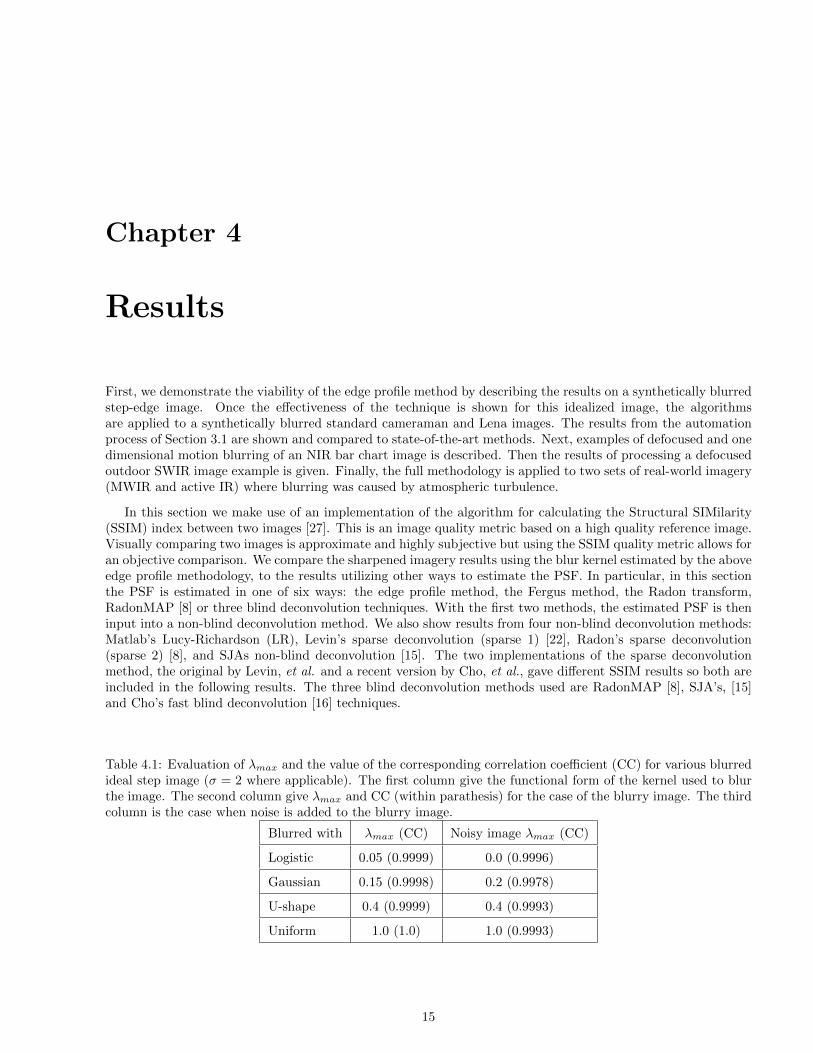
Table 4.1: Evaluation of λmax and the value of the corresponding correlation coefficient (CC) for various blurredideal step image (σ = 2 where applicable). The first column give the functional form of the kernel used to blurthe image. The second column give λmax and CC (within parathesis) for the case of the blurry image. The thirdcolumn is the case when noise is added to the blurry image.

Blurred with λmax (CC) Noisy image λmax (CC)

Logistic 0.05 (0.9999) 0.0 (0.9996)

Gaussian 0.15 (0.9998) 0.2 (0.9978)

U-shape 0.4 (0.9999) 0.4 (0.9993)

Uniform 1.0 (1.0) 1.0 (0.9993)

15

(a) (b)

Figure 4.1: Probability plots of Gaussian blurred ideal step edge. (a) Step edge images blurred with a Gaussiankernel with σ = 2, 4, 6, 8. (b) Step edge image blurred with a Gaussian kernel (σ = 6) and Gaussian white noiseadded (SNR = 35). The line is a linear LS fit to the data.

(a) (b)

Figure 4.2: PPCC plots for step-edge image with Gaussian white noise added (SNR=35). (a) blurred with aGaussian kernel, σ = 6. (b) blurred with a linear, uniform kernel of length 8 pixels.

4.1 Tests on an ideal step image

The effectiveness of the edge profile method is first demonstrated on a simple 256x256 step-edge image, wherethe left half = 0 and the right half = 1, which is then blurred with a Gaussian kernel with a known σ. In thecase with no noise, the transformed edge profile values fit perfectly to a straight line with the correct slope, asis shown in Fig. 4.1a for σ = 2, 4, 6, 8.

While it is clear that the method works when there is no noise, to be truly useful the method must prove tobe robust to noise. Gaussian white noise (SNR=35) was added to a Gaussian blurred step-edge image (σ = 6).Fig. 4.1b shows the plot of edge profile pixels along with a linear least squares fit to the data. Even though theestimated σ result did vary somewhat due to the noise, over numerous tests the estimated σ generally remainedwithin 3% of the the value used to blur the image. Furthermore, this accuracy was maintained over the range of

16

(a) (b) (c)

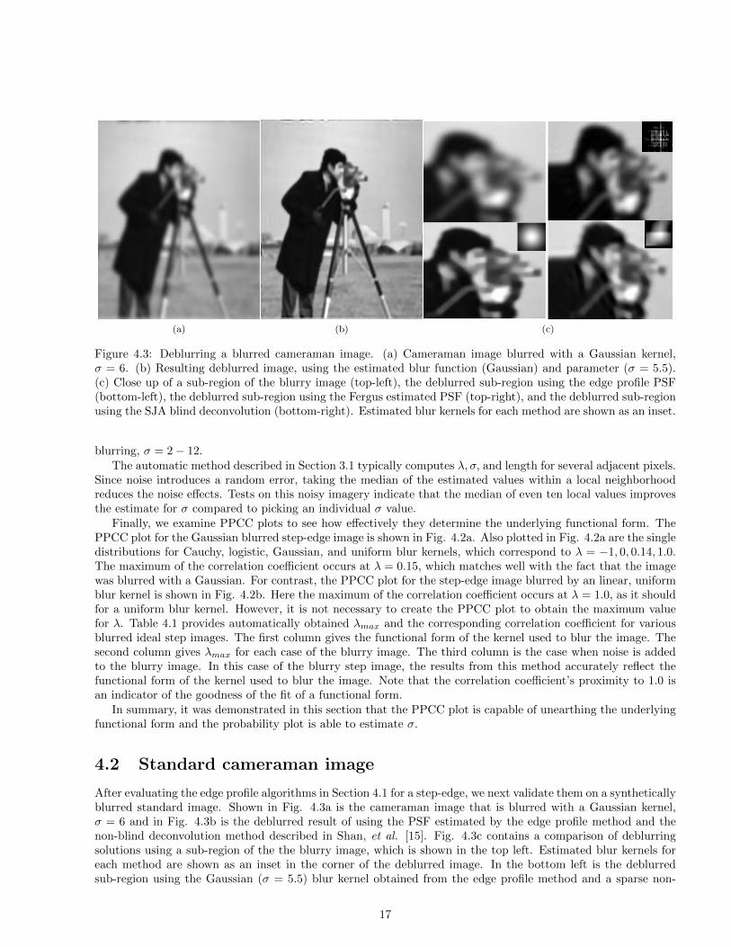
Figure 4.3: Deblurring a blurred cameraman image. (a) Cameraman image blurred with a Gaussian kernel,σ = 6. (b) Resulting deblurred image, using the estimated blur function (Gaussian) and parameter (σ = 5.5).(c) Close up of a sub-region of the blurry image (top-left), the deblurred sub-region using the edge profile PSF(bottom-left), the deblurred sub-region using the Fergus estimated PSF (top-right), and the deblurred sub-regionusing the SJA blind deconvolution (bottom-right). Estimated blur kernels for each method are shown as an inset.

blurring, σ = 2− 12.The automatic method described in Section 3.1 typically computes λ, σ, and length for several adjacent pixels.

Since noise introduces a random error, taking the median of the estimated values within a local neighborhoodreduces the noise effects. Tests on this noisy imagery indicate that the median of even ten local values improvesthe estimate for σ compared to picking an individual σ value.

Finally, we examine PPCC plots to see how effectively they determine the underlying functional form. ThePPCC plot for the Gaussian blurred step-edge image is shown in Fig. 4.2a. Also plotted in Fig. 4.2a are the singledistributions for Cauchy, logistic, Gaussian, and uniform blur kernels, which correspond to λ = −1, 0, 0.14, 1.0.The maximum of the correlation coefficient occurs at λ = 0.15, which matches well with the fact that the imagewas blurred with a Gaussian. For contrast, the PPCC plot for the step-edge image blurred by an linear, uniformblur kernel is shown in Fig. 4.2b. Here the maximum of the correlation coefficient occurs at λ = 1.0, as it shouldfor a uniform blur kernel. However, it is not necessary to create the PPCC plot to obtain the maximum valuefor λ. Table 4.1 provides automatically obtained λmax and the corresponding correlation coefficient for variousblurred ideal step images. The first column gives the functional form of the kernel used to blur the image. Thesecond column gives λmax for each case of the blurry image. The third column is the case when noise is addedto the blurry image. In this case of the blurry step image, the results from this method accurately reflect thefunctional form of the kernel used to blur the image. Note that the correlation coefficient’s proximity to 1.0 isan indicator of the goodness of the fit of a functional form.

In summary, it was demonstrated in this section that the PPCC plot is capable of unearthing the underlyingfunctional form and the probability plot is able to estimate σ.

4.2 Standard cameraman image

After evaluating the edge profile algorithms in Section 4.1 for a step-edge, we next validate them on a syntheticallyblurred standard image. Shown in Fig. 4.3a is the cameraman image that is blurred with a Gaussian kernel,σ = 6 and in Fig. 4.3b is the deblurred result of using the PSF estimated by the edge profile method and thenon-blind deconvolution method described in Shan, et al. [15]. Fig. 4.3c contains a comparison of deblurringsolutions using a sub-region of the the blurry image, which is shown in the top left. Estimated blur kernels foreach method are shown as an inset in the corner of the deblurred image. In the bottom left is the deblurredsub-region using the Gaussian (σ = 5.5) blur kernel obtained from the edge profile method and a sparse non-

17

(a) (b) (c)

Figure 4.4: Deblurring a blurred cameraman image with the Radon transform method. (a) User required edgeprofile length, sliceSize = 23. (b) User required edge profile length, sliceSize = 19. (c) RadonMAP method withuser required edge profile length, sliceSize = 23.

(a) (b) (c)

Figure 4.5: Parameter maps for a sub-region of blurred Cameraman image. The intensity scale is on the right-hand side and the intensity of the pixels correspond to their magnitude. (a) Lambda Map. (b) Sigma Map. (c)Length Map.

blind deconvolution method [22]. The Fergus estimated PSF [7] along with the sparse non-blind deconvolutionmethod produced the image in the top-right corner. The deblurred sub-region and blur kernel estimate in thebottom-right corner was obtained from the SJA blind deconvolution [15]. The results from four deconvolutionmethods, which are Richardson-Lucy (RL), two sparse implementation [22; 8] and SJA’s non-blind deconvolution,are visually similar.

The Radon transform method [8] was also used to deblur the cameraman image in Fig. 4.3a and the resultsare displayed in Fig. 4.4. The Radon transform parameter sliceSize, which is used as the profile length andPSF size, is a user supplied value and their results are strongly dependent on this value. In the author’s currentimplementation, this sliceSize parameter must be determined by a parameter search. However, based on theedge profile length, we choose sliceSize = 23 and produced the PSF and image shown in Fig. 4.4a. Thisdeblurred image displays strong ringing artifacts but a search of the parameter space for sliceSize and stdnoiseB(a smoothing parameter) lead to the improved image in Fig. 4.4b. Here the deblurred image contains fewerartifacts but the PSF is less similar to the Gaussian kernel that blurred the image. The RadonMAP method wasalso run on the blurry cameraman image and the results are shown in Fig. 4.4c. This deblurred image is betterand does not have ringing artifacts.

Column two in Table 4.2 gives SSIM scores for the deconvolved image compared to the original cameraman

18

Table 4.2: Mean SSIM quality metric of the deblurred images relative to an idealized reference.

Technique Blurry CM Noisy CM Blurry Lena Noisy Lena

No deblurring 0.707 0.725 0.680 0.810

Edge profile PSF / RL 0.815 0.756 0.774 0.858

Edge profile / Sparse 1 [22] 0.819 0.820 0.796 0.886

Edge profile / Sparse 2 [8] 0.790 0.825 0.780 0.884

Edge profile/SJA non-blind 0.721 0.796 0.783 0.868

Fergus PSF / RL 0.752 0.743 0.754 0.858

Fergus PSF / Sparse 1 0.753 0.789 0.762 0883

Fergus PSF / Sparse 2 0.749 0.803 0.762 0.875

Fergus PSF / SJA non-blind 0.723 0.795 0.747 0.847

Radon transform / Sparse 1 0.730 0.812 0.761 0.887

Radon transform / Sparse 2 0.777 0.810 0.759 0.874

RadonMAP / Sparse 1 0.772 0.822 0.732 0.886

RadonMAP / Sparse 2 0.768 0.824 0.734 0.874

SJA blind deconvolution 0.743 0.375 0.742 0.846

Cho’s blind deconvolution 0.682 0.714 0.716 0.804

Table 4.3: Summary of CPU times in seconds of each technique and imagery cited in this manuscript. CPUtime is cited running on a 2.4GHz Intel dual Core CPU on a T61 Thinkpad with 4GB RAM. In most cases,the Fergus PSF estimation run was performed on sub-regions of approximately 200x200, rather than on the fullimage.

Technique CM, Lena(512x512)

NIR(1024x1280)

SWIR(700x550)

MWIR(64x64)

Active IR(150x180)

Edge profile PSF 0.02 - 0.1 0.02 - 0.1 0.02 - 0.1 0.02 - 0.1 0.02 - 0.1

Fergus PSF[7] 970 1200 780 65 800

Sparse non-blind [22] 14 70 25 0.16 1.2

Matlab LR 6 51 9 .18 0.5

Matlab blind 13 120 20 0.26 1.6

SJA non-blind [15] 41 110 29 3 8

SJA blind [15] 65 240 62 6 12

Fast blind [16] 6.8 31 8.5 NA 1

Radon transform [8] 15 36 33 NA 16

RadonMAP [8] 150 NA NA NA 70

19

image. The SSIM index value between two images can be considered as the quality measure of an image if theother image (the reference) can be considered as perfect quality. If both images are identical the SSIM scoreequals 1.0 and goes to 0 as the match deteriorates. The blur kernels are estimated by the edge profile, Radontransform, RadonMAP, and the Fergus methods, then input to the four non-blind deconvolution method and theSSIM scores are listed in Table 4.2. In addition, the SJA and Cho’s blind deconvolution methods were run onthe blurry image and their scores listed in this table. In this case of the synthetically blurred cameraman image,the SSIM scores indicate that the edge profile method produces a better result, which is reasonable because thistest case is designed to match the underlying assumptions of Section 3.3.

It is possible to run an edge detection to create a map of edge pixels, then run the edge profile method onevery edge pixel. Doing this for the sub-region displayed in Fig. 4.3c one can create maps such as shown in Fig.4.5. These maps illustrate which pixels were accepted for computation by the automatic edge extraction methodand an estimate of its value (by its intensity) throughout the image. Experience has shown that it is usefulto look at these three maps on important horizontal and vertical edges when estimating the PSF because theyprovide an overall sense of PSF symmetry and the validity of the isoplanatic assumption; that is, this indicates ifit is reasonable to use a constant and/or symmetric PSF for the image. Fig. 4.5 indicates it is reasonable to usea constant PSF assumption for this image and the averages indicate the Gaussian functional form is appropriate.Grouping λ values in this map by direction of the edge one obtains an average λ = 0.17 for horizontal edgesand λ = 0.19 for vertical edges. Similarly, grouping σ values by direction of the edge one obtains an averageσ = 6.0 for horizontal edges and σ = 5.0 for vertical edges. This gives the estimate of σ = 5.5, which was usedto deconvolve the image. A map of edge profile lengths is shown in Fig. 4.5c and can be used to estimate thePSF support size that is appropriate. Grouping values by direction of the edge and we obtain an average length= 18.0 for horizontal edges and length = 15.0 for vertical edges. This implies that the effects of the Gaussianblurring is noticeable for about 15 - 18 pixels. However, the effects of the Gaussian function is primarily dictatedby σ and the support size just needs to be large enough. A rule of thumb is to make the PSF support size aboutfour times the σ value, which is about 22. For the result in Fig. 4.3 we used a 21x21 Gaussian PSF. Although thePSF estimated is not precise in this synthetically blurred example, the estimate reasonably matches the originalblur kernel.

Furthermore, the CPU times for the various software is listed in Table 4.3. An unoptimized Matlabimplementation of edge profile method executes orders of magnitude faster than any other method. The code tocompute correlation coefficients for a range of λ values, find the maximum λ, and determine σ from the quantilefunction executes in only 0.02 seconds CPU time and the function for finding strong edges and extracting theprofile runs in about 0.1 seconds (CPU time is cited running on a 2.4GHz Intel dual Core Thinkpad with 4GBRAM). This emphasizes the nature of the edge profile method as a quick but approximate (i.e., “back-of-the-envelope” or“quick and dirty”) that is useful in itself or as a quick check on more accurate methods. On theother hand, obtaining a blur kernel estimate using the Fergus method on a sub-region of 170x170 pixels takesabout 800 seconds. Please note that it is not a fair comparison to compare CPU times of a PSF estimationmethod to blind or non-blind deconvolution methods; the point to be made here is that the edge profile methodis a very fast in a field where all other methods are compute intensive. This speed advantage is one of the coreadvantages of the edge profile method. This method is valuable as a “quick and dirty” estimation of the blurkernel, which makes it attractive even when it’s performance is worse than the other methods. In addition, thismethod is preferable to guessing required in choosing a standard model and the searching of the parameter spacefor a best fit.

The presence of random noise in an image plagues attempts to deblur an image. As with all methods, theedge profile method is affected by noise and here we contrast the relative performance of this method to othermethods. In Fig. 4.6a the standard cameraman image was blurred with a Gaussian blur kernel with σ = 3and random, Gaussian white noise was added. Using the original cameraman image as the reference, this noisycameraman image gives a score of SSIM = 0.725. The automatic method for finding several high contrast edges,extracting these edge intensity profiles, yielded a large range of 0.0 < λmax < 0.4 and 2.1 < σ < 2.8. The errorin the automatic method is due primarily to errors in correctly determining edge profile end-points. Although,the automated method for extracting an edge profile starts to fail as the noise level increases, the edge profilemethod works well if one manually extracts edge profiles, which in this case correctly found λmax = 0.15 implyinga Gaussian blur function, with σ = 2.7. Hence, a 13x13 Gaussian blur kernel, with σ = 2.7 was used as inputto the non-blind deconvolution methods. The deblurred image is shown in 4.6c and the SSIM results shown incolumn three of Table 4.2.

20

(a) (b) (c)

Figure 4.6: Deblurring a noisy, blurred cameraman image. (a) Cameraman image blurred with a Gaussian kernel,σ = 3.0 with white noise added. (b) Resulting deblurred image, using the estimated blur function (Gaussian) andparameter (σ = 2.7). (c) Close up of a sub-region of the noisy, blurry image (top-left), the deblurred sub-regionusing the edge profile PSF (bottom-left), the deblurred sub-region using the Fergus estimated PSF (top-right),and the deblurred sub-region using the SJA blind deconvolution (bottom-right). Estimated blur kernels for eachmethod are shown as an inset.

(a) (b) (c)

Figure 4.7: Deblurring a noisy and blurry cameraman image with the Radon transform method with sliceSize =11. (a) Radon transform. (b) RadonMAP method. (c) Close up of a sub-region; top is Radon transform result,bottom is RadonMAP result.

Initially the Fergus PSF estimation worked poorly but with significant parameter tuning it was possible toobtain good results. Since each run of the Fergus method is computationally expensive, as shown in Table 4.3,this parameter search and testing of different sub-regions required many hours of computer time. The best resultis displayed in Fig. 4.6c. The SSIM results using this PSF as input to the four non-blind deconvolution methodsis shown in column three of Table 4.2. In addition to the parameter tuning, it is noteworthy that significantlydifferent blur kernels were obtained by running the Fergus method on different sub-regions. This variation islikely caused by the presence of the random noise.

The Radon transform and the RadonMAP results are displayed in Fig. 4.7. Some tuning of the implemen-tation’s stdnoiseB parameter was necessary to find the proper level for smoothing the noise but as can be seenin the figure, the results are good. This is also reflected in the SSIM scores in column three of Table 4.2. Table4.3 lists the CPU time for the Radon transform and RadonMAP methods. The speed of the Radon transform is

21

noteworthy as one of the faster blur kernel estimation methods, with the exception, of course, of the edge profilemethod.

The blind deconvolution blur kernel and resulting image for the SJA method are shown in Fig. 4.6c. Asvisible here, it is not unusual for the noise to be amplified in both the kernel and in the deblurred image. Table4.2 shows the SSIM scores for two blind deconvolution methods and it is clear that these methods have significantdifficulty in the presence of noise.

In summary, the presence of random noise caused the automated edge profile extraction to improperly estimatethe endpoints, leading to a wide range of parameter results. However, manually extracting an edge profile doeslead to identifying the correct blur kernel function and parameters. After significant parameter and sub-regiontuning the Fergus’s method was able to produce results of good quality. The Radon transform and RadonMAPmethods performed well, despite of the presence of the noise. But the two of the blind deconvolution methodsamplified the noise, leading to visibly worse results. The overall impression is that some methods are moresensitive to the presence of noise than others.

(a) (b) (c) (d)

Figure 4.8: (a) Gaussian blurred Lena image. (b) PPCC plot of Gaussian blurred Lena image. (c) Motionblurred Lena image. (d) PPCC plot of motion blurred Lena image.

(a) (b) (c) (d)

Figure 4.9: (a) Result from SJA non-blind deconvolution using a 27x27 Gaussian blur kernel with σ ' 5.4 (seeinset) from the edge profile PSF estimation. (b) Result from SJA non-blind deconvolution using the Fergus’sPSF estimation. (c) Result from SJA blind deconvolution. Inset shows estimated PSF. (d) Result from Cho’sFast blind deconvolution.

4.3 Standard Lena imagery

In this section, PSF estimators, non-blind and blind deconvolution methods are compared using a standard Lenaimage synthetically blurred with a known blur kernel. Shown in Fig. 4.8a is the result of blurring the Lenaimage with a Gaussian filter (σ = 6). A PPCC plot is used to model the functional form and is shown in 4.8b.

22

The maximum λmax = 0.15 implies a Gaussian functional form, as it should in this case. In contrast, Fig. 4.8cshows the Lena image blurred with a 16 pixel, linear uniform filter. Fig. 4.8d shows a PPCC plot from a verticaledge in the blurred image in Fig. 4.8c and the maximum about λmax ' 1 implies a uniform functional form.Hence, the PPCC plots do distinguish between different blurs.

(a) (b) (c) (d)

Figure 4.10: (a) Result from SJA non-blind deconvolution on noisy Lena image using a 12x12 Gaussian blur kernelwith σ = 2.6 (see inset) from the edge profile PSF estimation. (b) Result from SJA non-blind deconvolutionusing the Fergus’s PSF estimation (see inset). (c) Result from SJA blind deconvolution. Inset shows estimatedPSF. (d) Result from Cho’s Fast blind deconvolution. Inset shows estimated PSF.

Let’s look in more detail at analyzing the image in Fig. 4.8a. Automatically finding several high contrastedges, extracting these edge intensity profiles, and finding λmax via the PPCC plot gives a range of 0.05 <λmax < 0.15 for these edges. Or one can obtain an average of the λmax, σ, and length parameters over manystrong edges. Doing this gives λmax = 0.1, 0.15, σ = 5.1, 5.6, length = 26.5, 27 for vertical and horizontal edges,respectively. In both methods, the results imply a 27x27 Gaussian blur kernel, with σ ' 5.4. This exerciseillustrates that for images where a constant PSF assumption is valid, using a few strong edges will typically givesimilar results to averages over many edges but at a fraction of the computation time.

Fig. 4.9 shows four of the deblurred results of the image in Fig. 4.8a. It is easy to spot the differences in theblur kernels (inset in each image) but it is difficult to accurately compare the relative quality of the deconvolutionresults because the results are visually quite similar. But we can make a few observations. The SJA programsdo provide a smoothing parameter and some experimentation was performed. The value of the current settingwas necessary to remove image artifacts but the SJA results appear somewhat over-smoothed relative to otherdeblurred results The LR deconvolutions contain some ringing artifacts near the image boundaries even thoughthe function edgetaper was used as recommended by Matlab for minimizing this effect. The non-blind resultsusing the Gaussian PSF seem a bit sharper than the results using the Fergus PSF or the blind deconvolutionresults.

Using the original Lena image as a reference, the quality of these images can be reduced to numerical valuesand then compared. The fourth column in Table 4.2 lists the mean SSIM values for a variety of PSF anddeconvolution combinations, where the blurry Lena gives a score of SSIM = 0.680. Based on the SSIM score,the edge profile PSF estimation produced somewhat better deblurred results than Fergus’s method or the blinddeconvolution methods. As in the camerman example, this makes sense because this test case is designed tomatch the underlying assumptions of Section 3.3.

The edge profile method is affected by noise and here we contrast the relative performance of this methodto other methods. The standard Lena image was blurred with a Gaussian blur kernel with σ = 3 and random,Gaussian white noise was added. Using the original Lena image as the reference, this noisy Lena gives a scoreof SSIM = 0.810. Automatically finding several high contrast edges, extracting these edge intensity profiles,and finding λmax via the PPCC plot gives λmax ' 0.15 but with a larger range of −0.05 < λmax < 0.3 thanthe range from processing the purely blurry image. Or one can obtain an average over many strong edges ofλmax = 0.15, σ = 2.5, and length = 11. In this case it is reasonable to choose the Gaussian functional form,however when the image is polluted by noise there is increased uncertainty since range of these parameters islarger. As in the cameraman image case, manual edge profile extraction produces more accurate results, which

23

indicates the need for an improved automatic profile extraction methodology. Hence, a 13x13 Gaussian blurkernel, with σ = 2.6 was used as input to the non-blind deconvolution methods. The deblurred image is shownin 4.10a and the SSIM results shown in column four of Table 4.2.

The Fergus PSF estimation was run on various sub-regions of about 200x200 pixels and the best result isdisplayed in Fig. 4.10b. The SSIM results using this PSF as input to the three non-blind deconvolution methodsis shown in column four of Table 4.2. The CPU time for running the Fergus method on this sub-region is listedin Table 4.3.

Two blind deconvolution blur kernels and resulting images are shown in Figures 4.10c and 4.10d. As theSSIM scores in Table 4.2 shows, the Radon transform, RadonMAP, and SJA blind deconvolution are able toproduce results of similar quality to those produced using the edge profile PSF. The other methods’ scores sufferdue to the presence of noise.

The CPU times for the various software is listed in Table 4.3. Again this Matlab implementation of edgeprofile method executes orders of magnitude faster than any other method. This speed advantage is one of thecore advantages of the edge profile method. This method is valuable as a quick “back-of-the-envelope” estimationof the blur kernel as a check on, or an initial estimate of the kernel for more accurate methods, or simply toobtain an approximate PSF.

(a) (b) (c)

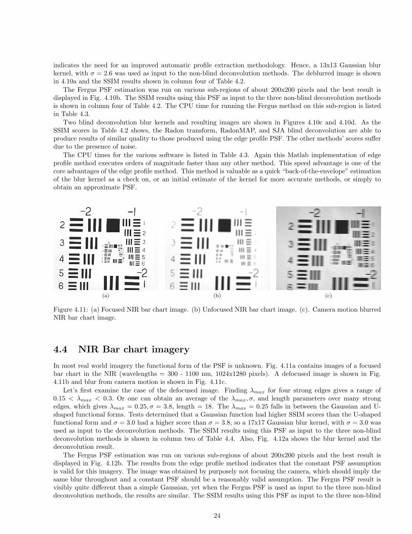
Figure 4.11: (a) Focused NIR bar chart image. (b) Unfocused NIR bar chart image. (c). Camera motion blurredNIR bar chart image.

4.4 NIR Bar chart imagery

In most real world imagery the functional form of the PSF is unknown. Fig. 4.11a contains images of a focusedbar chart in the NIR (wavelengths = 300 - 1100 nm, 1024x1280 pixels). A defocused image is shown in Fig.4.11b and blur from camera motion is shown in Fig. 4.11c.

Let’s first examine the case of the defocused image. Finding λmax for four strong edges gives a range of0.15 < λmax < 0.3. Or one can obtain an average of the λmax, σ, and length parameters over many strongedges, which gives λmax = 0.25, σ = 3.8, length = 18. The λmax = 0.25 falls in between the Gaussian and U-shaped functional forms. Tests determined that a Gaussian function had higher SSIM scores than the U-shapedfunctional form and σ = 3.0 had a higher score than σ = 3.8, so a 17x17 Gaussian blur kernel, with σ = 3.0 wasused as input to the deconvolution methods. The SSIM results using this PSF as input to the three non-blinddeconvolution methods is shown in column two of Table 4.4. Also, Fig. 4.12a shows the blur kernel and thedeconvolution result.

The Fergus PSF estimation was run on various sub-regions of about 200x200 pixels and the best result isdisplayed in Fig. 4.12b. The results from the edge profile method indicates that the constant PSF assumptionis valid for this imagery. The image was obtained by purposely not focusing the camera, which should imply thesame blur throughout and a constant PSF should be a reasonably valid assumption. The Fergus PSF result isvisibly quite different than a simple Gaussian, yet when the Fergus PSF is used as input to the three non-blinddeconvolution methods, the results are similar. The SSIM results using this PSF as input to the three non-blind

24

(a) (b)

(c) (d)

Figure 4.12: (a) Result from SJA non-blind deconvolution using a 17x17 Gaussian blur kernel with σ = 3 (seeinset), determined from the edge profile PSF estimation. (b) Result from SJA non-blind deconvolution using theFergus’s PSF estimation (see inset). (c) Result from SJA blind deconvolution. Inset shows estimated PSF. (d)Result from Cho’s Fast blind deconvolution. Inset shows estimated PSF.

deconvolution methods is shown in column two of Table 4.4. Fig. 4.12b shows the deconvolution result and theCPU time for running the Fergus method on this sub-region is listed in Table 4.3.

Two blind deconvolution blur kernels and resulting images are shown in Figures 4.12c and 4.12d. While eachblur kernel looks unique, the deconvolved images appear similar. Furthermore, these images all have similarSSIM scores. Hence the major distinction between all of these methods is CPU time, which is listed in Table 4.3and the edge profile method executes in a fraction of the time of the other methods.

Now let us examine the case of blurring by camera motion. Fig. 4.11c contains an image of the NIR bar chartblurred by camera motion. A PPCC plot of a vertical edge is shown in Fig. 4.13a along with the correspondingintensity profile that was used to create the PPCC plot. This vertical edge has a λmax = 1 but the horizontaledges have a λmax = 0, as can been seen by looking at a λ map of a sub-region that is shown in Fig. 4.13b. Acomparison of the lengths of vertical versus horizontal edge profiles also illustrate this asymmetry; vertical edgeprofiles span about 30 to 38 pixels while a horizontal edge profile is only around 4 to 6 pixels. Essentially this

25

(a) (b)

Figure 4.13: (a) Edge intensity profile and PPCC plot for a vertical edge from image shown in Fig. 4.11c. (b) λMap of bar chart with camera motion. Shows that λ ' 1 for vertical edges and λ ' 0 for horizontal edges.

Table 4.4: Mean SSIM quality metric of the deblurred images relative to an idealized reference.

Technique Unfocused NIR Motion NIR SWIR MWIR Active IR

No deblurring 0.772 0.728 0.819 0.839 0.623

Edge profile PSF / RL 0.803 0.772 0.864 0.894 0.743

Edge profile / Sparse 1 0.806 0.756 0.856 0.885 0.698

Edge profile / Sparse 2 0.781 0.865 0.860 0.847 0.668

Edge profile/SJA non-blind 0.778 0.712 0.833 0.014 0.660

Fergus PSF / RL 0.798 0.726 0.795 0.880 0.630

Fergus PSF / Sparse 1 0.817 0.782 0.853 0.885 0.632

Fergus PSF / Sparse 2 0.780 0.732 0.800 0.878 0.620

Fergus PSF / SJA non-blind 0.770 0.678 0.705 0.013 0.646

Radon transform / Sparse 1 0.784 0.758 0.833 NA 0.691

Radon transform / Sparse 2 0.777 0.858 0.907 NA 0.664

RadonMAP / Sparse 1 0.832 NA 0.831 NA 0.693

RadonMAP / Sparse 2 0.777 NA 0.901 NA 0.664

SJA blind deconvolution 0.759 0.617 0.735 0.016 0.647

Cho’s blind deconvolution 0.784 0.721 0.792 NA 0.584

implies a horizontal, uniform, linear PSF of length 30 to 38 pixels (obviously σ is not relevant for a uniform blurkernel). A few tests showed that a linear blur kernel of length 31 produced better results than longer kernelsso this is the kernel used to produce the result shown in Fig. 4.14a. Furthermore, comparisons of LR andsparse deconvolution results using 1-D Uniform, U-shape, Gaussian, and logistic PSFs of various sizes showedthat a 33 pixel uniform function produces the sharpest edges, which confirms this result. The SSIM scores fordeconvolution with this kernel is given in column two of Table 4.4. The scores for the edge profile estimated

26

(a) (b)

(c) (d)

Figure 4.14: (a) Result from SJA non-blind deconvolution using a 33 pixel, uniform, linear blur kernel asdetermined from the edge profile PSF estimation. (b) Result from SJA non-blind deconvolution using the Fergus’sPSF estimation. (c) Result from SJA blind deconvolution. (d) Result from Cho’s Fast blind deconvolution.

Table 4.5: Mean SSIM metric of the motion blurred image using the Radon transform PSF of various values forsliceSize (from 29 to 45) with the two sparse deconvolution methods. Significantly different results were obtainedfrom the sparse deconvolution of [8] than the original implementation by [22].

Technique 29 31 33 35 37 39 41 43 45 47 49

Sparse 2 [8] 0.871 0.883 0.845 0.879 0.880 0.782 0.863 0.757 0.790 0.737 0.765

Sparse 1 [22] 0.753 0.758 0.738 0.728 0.760 0.727 0.734 0.701 0.758 0.745 0.760

PSFs are similar to the other methods in spite of the ringing and ghosting artifacts in the edge profile result andis perhaps helped by some smoothing by the non-blind deconvolution method.

The Fergus, Radon Transform, RadonMAPP, SJA and Cho’s fast blind deconvolution methods are all geared

27

(a) (b)

Figure 4.15: (a) Result from Sparse non-blind deconvolution using a 31x31 Radon transform blur kernel (seeinset). (b) Result from SJA non-blind deconvolution using the Fergus’s PSF estimation (see inset).

towards deblurring camera shake that causes motion blur. Hence, it should be expected that these methodsperform well for this imagery. However, the SSIM scores for the results of deblurring this image, which aregiven in column two of Table 4.4, show that the simple edge profile PSF obtains comparable results. On theother hand, close examination of the deblurring results of this linear filter to the other deconvolution resultsshow that the edge profile results contain sharper edges but also more ringing and ghosting artifacts. This resultillustrates an important difference between this edge profile blur kernel estimation and other methods. PreviousPSF estimation and blind deconvolution methods have the dual aims to restore edge sharpness and noise/artifactsuppression in homogeneous regions; however, the only goal inherent in the edge profile method is restoring edgesharpness, ideally to step-edges. That is, the results of non-blind deconvolution for the edge profile blur kerneltends to have have both sharper edges and more artifacts than the other methods.

The Fergus PSF estimation was run on various sub-regions of size about 200x200 and the best result isdisplayed in Fig. 4.15b. The estimated PSF is nearly linear and yet it seems this PSF does only a little tosharpen edges. Fig. 4.14c presents the deblurring results for the SJA blind deconvolution method and here it isclear the estimated PSF is nearly linear. Similarly for Cho’s fast blind deconvolution results shown in Fig. 4.14d,however the method seems to over smooth parts of the image and appears to be of poor quality. Also, keep inmind that it is likely that the scores for the edge profile estimated PSFs are lowered because of the ringing andghosting artifacts.

This image was input to the Radon transform method and the results were somewhat inexplicable. When themethod was run with the original code, including their sparse deconvolution, the resulting image was significantlybetter than any other method (see Fig. 4.15a). However, saving the same PSF and running with Levin’s sparsedeconvolution produced poor results. This can be seen in the results contained in column three of Table 4.4 andeven more clearly in Table 4.5, which compares the two sparse deconvolution methods over a range of sliceSizevalues. I examined the code and experimented with a variety of parameters values, yet was not able to explainthese results. Furthermore, there does not seem to be a logical pattern in Table 4.5 correlating the SSIM valueto the values of sliceSize. However, some of the better SSIM values using the sparse deconvolution of [8] wereobtained for sliceSize in the range of 31 to 37, which corresponds nicely to the length of the edge profiles citedabove. Several attempts to run the RadonMAP program failed to complete executing so no results were obtained.

It is also noteworthy that image registration is necessary before computing a SSIM score because the longkernel can significantly shift the edge location relative to the focused reference image. Subsequently, sub-pixelregistration method was then used to obtain SSIM scores for all the imagery in Tables 4.2 and 4.4, even thoughfor most of the other imagery the shift was small.

28

(a) (b)

Figure 4.16: (a) Focused SWIR image. (b) Unfocused SWIR image.

(a) (b) (c) (d)

Figure 4.17: (a) Result from SJA non-blind deconvolution using an 11x11 logistical blur kernel with σ = 1.5 (seeinset), as determined from the edge profile PSF estimation. (b) Result from SJA non-blind deconvolution usingthe Fergus’s PSF estimation (see inset). (c) Result from SJA blind deconvolution. Inset shows estimated PSF.

4.5 Outdoor SWIR imagery

Fig. 4.16a shows a focused SWIR image (wavelengths = 0.9 - 1.7 um, 700x550 pixels) and Fig. 4.16b showsan unfocused version of the same scene. Finding λmax for four strong edges gives a range of 0 < λmax < 0.2.Or one can obtain an average of the λmax, σ, and length parameters over many strong edges, which givesλmax = 0.2, σ = 3, length = 11. The λmax ' 0.2 implies the Gaussian functional form with σ = 3.0, which testsconfirm. For the results given in this section, a 13x13 Gaussian with σ = 3.0 was used. The SSIM results usingthis PSF as input to the four non-blind deconvolution methods is shown in column four of Table 4.4. Also, Fig.4.17a shows the blur kernel and the deconvolution result.

29

The Fergus PSF estimation was run on various sub-regions of about 200x200 pixels and the best result isdisplayed in Fig. 4.17b. The Fergus PSF result is visibly quite different than a simple Gaussian, yet when theFergus PSF is used as input to the non-blind deconvolution methods, the results are quite similar. The SSIMresults using this PSF as input to the four non-blind deconvolution methods are also shown in column four ofTable 4.4. Fig. 4.17b shows the deconvolution result and the CPU time for running the Fergus method is listedin Table 4.3. The Radon transform and RadonMAP methods both work well and produce good quality results.

Two blind deconvolution blur kernels and resulting images are shown in Figures 4.17c and 4.17d. Theseimages appear to be very similar and all have similar SSIM scores, as can be seen in Table 4.4. The differencesin SSIM scores are more related to the amount of smoothing done by the non-blind deconvolution method ratherthan related to the differences in the input blur kernel. Hence the major distinction between all of these methodsis CPU time, which is listed in Table 4.3. The SWIR image is one of the larger images studied in this research,hence the CPU difference between methods is more pronounced.

4.6 Tests on atmospheric turbulence blurred imagery

Applying these algorithms to real-world imagery is an important test. One ubiquitous cause of blurring is fromatmospheric turbulence, which often imposes a practical limit on the performance of imaging sensor systems[28]. Two videos demonstrating atmospheric turbulence blurring effects were provided courtesy of the NightVision and Electronic Sensors Directorate (US Army RDECOM CERDEC NVESD). The first image sequencewas collected at a mid-Atlantic US Army Test Site on September 2008 using a L3/CE 640x512x28µm MWIRsensor, and this video contains distortion and warping along with the blurring. The second is an active IR videosequence recorded at a closed test site, which has significant noise and speckle artifacts. Both these problemsare mitigated by averaging several frames; 10 frames for the first sequence and 50 for the second. The averagedimages are displayed in Fig. 4.18 and these images were used in the investigations discussed in this section.Although there aren’t references for these image, ideal reference images shown in Fig. 4.19 were created in orderto compute SSIM values . For the MWIR image the SSIM score of the target area from the original image wascomputed to be 0.839. The reference for the active IR image consisted of white squares and rectangles on ahomogeneous dark background and an effort was made to align the reference with the image. The SSIM scoreof the the image in Fig. 4.18 to this reference is 0.623.

MWIR imagery

Automatic extraction of the edge profiles had some variability, giving a range of results of 0 < λmax < 0.3, 2.3 <σ < 2.8, and length between 10 and 14 pixels. However, manual extraction of several edge profiles from Fig.4.18a gave λmax = 0.1, σ = 2.3, and length of 12 pixels. Either a Gaussian or a logistical function fits withinthis range and our tests showed that the logistical blur kernel performed a little better than a Gaussian PSF.Fig. 4.20a shows the results of non-blind sparse deconvolution using a 11x11 logistical PSF with σ = 2.

In Fig. 4.20b is the result of the Fergus PSF estimation and the results of non-blind sparse deconvolution.Examination of the SSIM scores in Table 4.4 show similar results are obtained from both methods. However, asseen in Table 4.3, the CPU times for the edge profile method is a fraction of the time for the Fergus method. Dueto the lack of edges in this image, the Radon transform and RadonMAP methods failed in most attempts andwhen it was possible to produce a result, it was of very poor quality. Attempts to deconvolve this image withSJA blind and non-blind deconvolution produced poor results, which can be seen in Fig. 4.20c and are reflectedin the SSIM scores. In addition, it was not possible to obtain a result with Cho’s blind deconvolution, even overa range of parameter settings. This image demonstrates the robustness of the edge profile method because it ispossible to obtain an approximate blur kernel with difficult imagery; it simply requires manually extracting theprofile rather than relying on the automatic profile extraction.

Active IR imagery

The active IR image in Fig. 4.18b is a difficult problem because active IR is prone to significant image artifacts,including noise and speckle effects. It is instructive to examine the λ and σ maps for this image, which areshown in Fig. 4.21. It appears in the map that λ shows significant variation due to noise, which implies that the

30

(a) (b)

Figure 4.18: (a) MWIR collect at a US Army Test Site on September 2008. Displayed image is an average of thefirst 10 frames. (b) Displayed image is a sub-region containing one of the targets from a closed test site. It wastaken with an Active IR sensor. The displayed image is an average of 50 frames to reduce the noise inherent inactive IR imagery.

(a) (b)

Figure 4.19: (a) MWIR reference image for SSIM comparison. (b) Active IR reference image.

assumption of a constant blur kernel is poor for this image. But the constant PSF assumption was used for thesake of continuing the comparison with the deconvolution methods used so far in this report.

Finding λmax for four strong edges gives a wide range of −0.05 < λmax < 0.25, where each of these four edgegave a different value. Closer examination of the results indicates that the best edge profile gives λmax = 0.05.Looking at averages from the automatic evaluation of the edge profiles in the image gives λ = 0.05 and anaverage value of σ is in the range from 2.0 to 2.9. Manual extraction of several edge profiles give λmax = 0.05 to0.1, σ = 2.3, and length of 13 to 15 pixels., which can imply either a Gaussian or logistic functional form. Testsshow that either functional form produced similar results but the logistical function requiring a larger value forσ of approximately 3.0. So a 13x13 Gaussian blur kernel with σ = 2.4 was used to produce the result in Fig.4.22a.

In Fig. 4.22b is the result of the Fergus PSF estimation and the results of non-blind SJA deconvolution. Also,Table 4.3 gives a comparison of the CPU times, where the edge profile method again requires a fraction of thetime the other methods need. Two blind deconvolution blur kernels and resulting images are shown in Figures

31

(a) (b) (c)

Figure 4.20: PSF estimation (corner insert) and non-blind sparse deconvolution for the MWIR image. (a) Edgeprofile estimation of a 11x11 logistical blur kernel. (b) Fergus PSF estimation. (c) SJA blind deconvolution.

(a) (b)

Figure 4.21: (a) λ map for Active IR image. (b) σ map.

4.22c and 4.22d. The Radon transform and RadonMAP methods were also run on this image and the resultsappear visually similar to the Fergus PSF results but the SSIM scores in Table 4.4 are somewhat higher. It canbe seen that the SSIM values in column five of Table 4.4 also are similar, so once again it is the CPU time thatprimarily differentiates the methods.

The inconsistency of the results shown in Fig. 4.22 and SSIM scores in Table 4.4 require some discussion.Cho’s fast deblurring method obtains a relatively high SSIM score but the image displayed in Fig. 4.22d isvisibly of poorer quality than the other images. This is caused by the simple choice for a reference image touse homogeneous light regions on a homogeneous dark background. The smoothing performed by Cho’s fastdeblurring method creates a result that most resembles this reference. There might be times when this resultis desirable but for our purposes this seems to be a poor visual result. The results in Figures 4.22a and 4.22bagain illustrate the difference between this edge profile blur kernel estimation and other methods; that is, othermethods have the dual aims to restore edge sharpness and noise/artifact suppression in homogeneous regions,while the only goal inherent in the edge profile method is restoring edge sharpness.

32

(a) (b)

(c) (d)

Figure 4.22: (a) Result from SJA non-blind deconvolution using a 15x15 logistic blur kernel with σ = 3 (seeinset), as determined from the edge profile PSF estimation. (b) Result from SJA non-blind deconvolution usingthe Fergus’s PSF estimation (see inset). (c) Result from SJA blind deconvolution. Inset shows estimated PSF.(d) Result from Fast blind deconvolution. Inset shows estimated PSF.

4.7 Limitations

As with any methodology, there are boundaries beyond which this approach is not practical. It is outside thecapability of the edge profile method to determine random blur kernels found in the camera motion deblurringliterature such as [7], [16], [15], [21]. Furthermore, initial tests with imagery blurred by these complex blur kernelsshowed that the edge profile method performed poorly relative to the Fergus method. The complex kernels inthe motion blur literature generally have non-analytic shapes, random values and are not symmetrical. Hence,based on the assumptions described in Section 3.3, this is beyond the capability of this method. On the otherhand, it is possible to use a fast edge profile PSF estimation for an initial guess to be input into more accuratePSF estimation or blind deconvolution techniques, such as in [7], [16], [15], [21], in order to produce faster andflexible techniques. This topic is a candidate for future research.

As mentioned above, the edge profile method aims only to sharpen edges while other methods have the dualgoals of sharper edges and reducing noise/artifacts in smooth regions. In addition, there are some approximationsin the automation of this method that may introduce errors and limit the accuracy of the result in the presenceof noise. For example, this method relies primarily on differences between shapes of the profile. During thisstudy it was noticed that the greater the blurring or more noise present, the more difficult it is to distinguishbetween functional forms. This effect was present in the results described in Sections 4.2 and 4.6. On the otherhand, in these cases the deconvolution results from different functional forms are similar and the edge profilemethod still provides reasonable parameter values.

Furthermore, the methods for determining the endpoints of the blurry edge profile are approximate and anincorrect edge profile can introduce error into blur kernel estimates. Also, for the work presented in this report,noise hindered the automatic endpoint estimation and occasionally required manual edge profile extraction.However, it is hoped that the automated implementation will become more robust in the course of time.

33

Chapter 5

Conclusions

This report shows how to estimate the blur kernel directly from a blurry image by using the concepts behindquantile-quantile plots, probability plots, and probability plot correlation coefficient plots. Finding the shapeparameter that yields the maximum probability plot correlation coefficient indicates the best functional form forthe blur kernel. Given the functional form of the blur kernel, the parameters are obtained from a straight linefit to the transformed edge profile, eliminating any searching of the parameter space. Maps provide insight tothe asymmetry and spatial variation in an image’s blurring, allowing an informed decision on whether to use anisoplanatic or anisoplanatic, symmetric or asymmetric PSF. These methods are non-iterative, simple, and robustto noise.

Although most of the Results section is spent comparing the edge profile method to state-of-the-art methods,this method is best compared to PSF selection by standard models. In the standard model method one guesses ata functional form and parameters based on a prior knowledge of the blurring or one searches the parameter spaceto estimate the parameters. Instead, the edge profile method shows how to quickly estimate the functionalform and parameters from blurry edges in the image. We show in the Results section that a blur kernelestimated in such a simple manner produces deconvolution results of similar quality to the results from muchmore computationally intensive state-of-the-art deconvolution methods.

This work opens up several areas for future research. One area is to obtain more versatile and accurateblur kernels through the use of other blur functions or a mixture of functions [26] [25]. Secondly, the edgeprofile method can be integrated with a more accurate PSF estimation or blind deconvolution method. Finally,integrating the edge profile method with a spatially varying deconvolution method will take advantage of bothits qualities of speed and locality.

Image deblurring is a building block for many other techniques. Atmospheric turbulence mitigation wasstudied in this report but this methodology could be applied to a number of applications. For example, thismethod is particularly suited for the deblurring step of super-resolution methods because it defines a continuousfunction for the blur kernel, and hence can be defined at any desirable resolution.

Acknowledgment

The author would like to thank the Office of Naval Research for their support of this research and RichardEspinola at US Army RDECOM CERDEC NVESD for supplying the imagery used in this investigation. Inaddition, the author thanks Colin Olson of NRL for his comments on this report and all the researchers whomade their programs available.

34

Bibliography

[1] Hugh G. Gauch, Scientific method in practice, Chapter 7, Cambridge University Press, 2003.

[2] Richard W. Hamming, The art of doing science and engineering : learning to learn, Chapter 1, Gordon andBreach, 1997.

[3] Reginald L. Lagendijk and Jan Biemond, Basic Methods for Image Restoration and Identification, Chapter3.5, Handbook of image and video processing, Editor Al Bovik, Academic Press, 2000.

[4] D. Kundur and D. Hatzinakos, “Blind image deconvolution”, IEEE Signal Processing Magazine, 1996.

[5] Anat Levin, Yair Weiss, Fredo Durand, William T. Freeman, “Understanding and evaluating blinddeconvolution algorithms”, IEEE Computer Society Conference on Computer Vision and PatternRecognition, CVPR’09, 2009.

[6] Leslie N. Smith, James R. Waterman and K. Peter Judd, ”A new blur kernel estimator and comparisons tostate-of-the-art”, Proc. SPIE 8014, 80140N (2011); doi:10.1117/12.888126.

[7] R. Fergus, B. Singh, A. Hertzmann, S.T. Roweis, and W.T. Freeman “ Removing camera shake from asingle photograph”, SIGGRAPH, 2006.

[8] Taeg S. Cho, Sylvain Paris, Berthold K.P. Horn, William T. Freeman, “Blur kernel estimation using theRadon transform”, IEEE Computer Society Conference on Computer Vision and Pattern Recognition,CVPR’11, 2011.

[9] N. Joshi, R. Szeliski, and D. Kriegman, “PSF estimation using sharp edge prediction”, IEEE ComputerSociety Conference on Computer Vision and Pattern Recognition, CVPR’08, 2008.

[10] Ming-Chao Chiang, Terrance E. Boult, “Local Blur Estimation and Super-Resolution”, IEEE ComputerSociety Conference on Computer Vision and Pattern Recognition (CVPR’97), pp.821, 1997.

[11] E.H. Barney-Smith, “PSF estimation by gradient descent fit to the ESF”, SPIE Image Quality and SystemPerformance III,Vol. 6059, 2006.

[12] V. Kayargadde and J.-B. Martens, “Estimation of edge parameters and image blur using polynomialtransforms”, CVGIP Graphical Models Image Process., 56, 442461, 1994.

[13] B. Chalmond, “PSF Estimation for Image Deblurring”, CVGIP: Graphical Models and Image Processing,Vol. 53, No. 4, pp. 364-372, 1991.

[14] Azriel Rosenfeld, Avinash Kak, Digital Picture Processing, Academic Press, 1982.

[15] Q. Shan, J. Jia, A. Agarwala, “Highquality Motion Deblurring from a Single Image”, ACM Trans. Graph.27, 3, Article 73, August 2008.

[16] Sunghyun Cho, Seungyong Lee “Fast Motion Deblurring”, Proceedings of SIGGRAPH ASIA , 28, 5,December 2009.

[17] T. J. Schulz, “Multiframe blind deconvolution of astronomical images”, J. Optical Soc. Amer., 10, pg.10641073, 1993.

35

[18] L. Yuan, J. Sun, L. Quan,H. Shum, “Image deblurring with blurred/noisy image pairs”, ACM Trans. onGraph. (SIGGRAPH) 26, 3, 110, 2007.

[19] W. Richardson, “Bayesian-based iterative method of image restoration”, Journal of the Optical Society ofAmerica A 62, 1972.

[20] L. Lucy, “An iterative technique for the rectification of observed distributions”, Journal of Astronomy,Volume 79, number 6, pages 745-754, 1974.

[21] L. Yuan, J. Sun, L. Quan,H. Shum, “Progressive Interscale and Intrascale Nonblind Image Deconvolution”,ACM Trans. Graph. 27, 3, Article 74, August 2008.

[22] A. Levin, R. Fergus, F. Durand, and W. Freeman, “Image and depth from a conventional camera with acoded aperture”, SIGGRAPH, 2007.

[23] James J. Filliben, “The Probability Plot Correlation Coefficient Test for Normality”, Technometrics, Vol.17, No. 1, pp. 111-117 (Feb., 1975).

[24] John Chambers, William Cleveland, Beat Kleiner and Paul Tukey, Graphical Methods for Data Analysis,Chapter 6, Wadsworth and Brooks, 1983.

[25] Zaven A. Karian and Edward J. Dudewicz, Fitting Statistical Distributions: The Generalized LambdaDistribution and Generalized Bootstrap Methods, CRC Press, 2000.

[26] Warren Gilchrist, Statistical Modelling with Quantile Functions, Chapman and Hall/CRC, 2000.

[27] Z. Wang, A. C. Bovik, H. R. Sheikh, and E. P. Simoncelli, “Image quality assessment: From error visibilityto structural similarity,” IEEE Transactions on Image Processing, vol. 13, no. 4, pp. 600-612, Apr. 2004.

[28] Richard L. Espinola, Jae Cha, and Kevin Leonard, “Novel methodologies for the measurement of atmosphericturbulence effects”, Proc. SPIE 7662, 76620W, 2010.

Biography

Leslie N. Smith received a Ph.D. degree in chemical physics from the University ofIllinois in 1979. He currently works for the Naval Research Laboratory in Washington, D.C. as a memberof the Maritime Sensing Section in the Optical Sciences Division on real-time image processing and targetdetection, tracking applications. His research interests include real-time video processing, image restoration,image enhancement (high dynamic range compression, contrast enhancement, super-resolution), use of GPUs inimage processing, threat detection (image registration, automatic object detection, background modeling, changedetection, tracking, object segmentation, classification) and automatic image understanding.

36