1

Estimating behavior in a black box: How coastal oceanographic dynamics influence yearling Chinook salmon marine growth and migration behaviors

Brian J. Burke1*, James J. Anderson2, Jessica A. Miller3, Londi Tomaro3, David J. Teel4, Neil S.

Banas5, and Antonio M. Baptista6

1NOAA Fisheries, Northwest Fisheries Science Center, Fish Ecology Division, Seattle, WA

98125 2University of Washington, School of Aquatic and Fishery Sciences, Seattle, WA 98105 3Coastal Oregon Marine Experiment Station, Hatfield Marine Science Center, Department of

Fisheries and Wildlife, Oregon State University, Newport, OR 97365 4NOAA Fisheries, Northwest Fisheries Science Center, Conservation Biology Division,

Manchester, WA 98353 5University of Strathclyde, Department of Mathematics and Statistics, Glasgow, G1 1XQ, UK 6Center for Coastal Margin Observation & Prediction, Oregon Health & Science University,

Beaverton, OR 97006

* Corresponding Author Email: brian.burke@noaa.gov Phone: 206-860-3486 Fax: 206-860-3267

2

Abstract Ocean currents or temperature may substantially influence migration behavior in many

marine species. However, high-resolution data on animal movement in the marine environment

are scarce; therefore, analysts and managers must typically rely on unvalidated assumptions

regarding movement, behavior, and habitat use. We used a spatially explicit, individual-based

model of early marine migration with two stocks of yearling Chinook salmon to quantify the

influence of external forces on estimates of swim speed, consumption, and growth. Model

results suggest that salmon behaviorally compensate for changes in the strength and direction of

ocean currents. These compensations can result in salmon swimming several times farther than

their net movement (straight-line distance) would indicate. However, the magnitude of

discrepancy between compensated and straight-line distances varied between oceanographic

models. Nevertheless, estimates of relative swim speed among fish groups were less sensitive to

the choice of model than estimates of absolute individual swim speed. By comparing groups of

fish, this tool can be applied to management questions, such as how experiences and behavior

may differ between groups of hatchery fish released early vs. later in the season. By taking into

account the experiences and behavior of individual fish, as well as the influence of physical

ocean processes, our approach helps illuminate the "black box" of juvenile salmon behavior in

the early marine phase of the life cycle.

Keywords: Chinook salmon, oceanographic model, individual-based model, behavior,

marine migration

3

Introduction Although scientists have long considered the ocean a “black box” in terms of animal ecology, technological advances over the past few decades have greatly improved our understanding of movement, behavior, and survival in marine organisms (Hussey et al. 2015). In particular, technologies that can associate the location or movement of an animal with environmental data have supported new mechanistic descriptions of animal behavior (Cooke et al. 2004). Even so, study of the marine environment is limited by fiscal and technological constraints, particularly for small organisms. For many small pelagic marine fishes, such as juvenile salmonids that have recently entered the marine environment, the mechanisms driving behavioral choices are still poorly understood. We know that predators, prey, and abiotic variables are spatially and temporally heterogeneous (Emmett et al. 2001, Brodeur et al. 2011, Ruzicka et al. 2012). Therefore, a better understanding of behavioral ecology in the ocean will require additional information on animal locations and their environmental experiences.

Quantitative tools play an essential role in estimating fish movement (Byron and Burke 2014). For a limited number of species, mark-recapture methods such as coded-wire tagging have provided some basic information (Weitkamp 2010, Fisher et al. 2014). However, for most species, data from marking studies are not forthcoming. Oceanographic models may expand our understanding of marine ecology and broaden the scope of available movement data for these stocks and species. Once created and validated, these tools may be applied to more detailed questions, such as how organisms might adjust their behavior or phenology as marine environments change (Anderson et al. 2013).

For migrating species, environmental experiences are defined as much by animal movement as by the availability and spatial distribution of quality habitat. Movement of a migrating species is complex and highly dynamic over space and time. To understand behaviors employed or stimuli used by migrating fish, movement dynamics must be estimated with fairly high precision (e.g., hourly or daily). However, many estimates of fish movement rely solely on net distance and speed between capture/release and recapture locations, assuming a straight-line trajectory (Thorstad et al. 2007, Welch et al. 2009, Welch et al. 2011, Tomaro et al. 2012). While such information is useful for characterizing spatial distributions, it cannot resolve the ecological and behavioral processes involved in a fish moving between two locations.

We used an individual-based model of fish movement and behavior to estimate swim speeds and growth rates in coastal waters. By taking into account time-varying external forces, such as ocean currents, and the entire time series of environmental experiences, we were able to estimate behavioral responses to the environment at any point along a migration segment. We applied this coupled biophysical model to yearling Chinook salmon from the Columbia River Basin, including stocks listed as threatened and endangered under the U.S. Endangered Species Act (NOAA 1992).

4

While the resolution and detail of oceanographic models have increased greatly over the past decade, results often differ depending on the specific models used, the spatial extent and grain (i.e., cell size), and boundary conditions. Validation of large oceanographic models is often limited, so it is important to identify which model or model configuration best describes the environment fish experience during migration. Therefore, our approach was to represent the physical environment with multiple models, and then to characterize the sensitivity of specific migration behaviors to differences in the physical environment. Using this approach, we hoped to identify critical behaviors used by juvenile salmon during ocean migration. In a larger framework, we demonstrated the feasibility of this approach in characterizing marine migratory behavior for other stocks and species.

Methods We combined multiple data types to synthesize the best estimate of salmon migration and environmental experiences. We used this information in a simulation tool to determine the effect of various behavioral rules on migration rates and routes, swim speeds, and growth rates. Although we did not expect to precisely estimate migration behavior, we put bounds on the potential behaviors by using empirical data to ground the simulations. Below, we describe the data sources, models, and results from simulations.

YearlingChinookSalmonDataOur analysis was based on data from an ongoing study of juvenile salmon spatial distributions (Jacobson et al. 2012, Teel et al. 2015). Six to seven stations along transects extending outward from the coasts of Washington and Oregon were sampled during 20-30 May and 18-30 June from 2003 through 2008. Because few fish were collected in 2005, we used only data from 2003-2004 and 2006-2008. At each station, a Nordic 264 pelagic rope trawl (30 × 20 × 200 m) with a cod-end liner of 9.5-mm stretch mesh was towed at a speed of 6 km·h-1 for approximately 30 min. (see Krutzikowsky and Emmett 2005 for complete details).

OtolithAnalysisA subsample of the juveniles collected in trawl surveys was selected for otolith structural and chemical analyses to determine size at and time of freshwater outmigration, as well as marine growth and migration rates (Tomaro et al. 2012, Miller et al. 2013). Sagittal otoliths were removed, cleaned, and polished using wet-or-dry paper (240-2500 grit) and lapping film (1-30 µm) using standard procedures for elemental analysis (Miller 2009). Otolith Sr and Ca were measured along the dorsal-ventral growth axis using laser ablation-inductively coupled plasma mass spectrometry.

The laser was set at a pulse rate of 7 Hz and translated across the sample at 5 µm s-1 with a spot size of 30 or 50 µm. Normalized ion ratios were converted to molar ratios using standard procedures (Kent and Ungerer 2006, Miller 2009). Instrument precision (mean percent relative standard deviation) was <5% for Ca and Sr across all samples and days (n = 65), and accuracy of

5

the Sr:Ca ratio was 4% (n = 10) based on microanalytical reference material (MACS-1, U.S. Geological Survey).

Image analysis combined with Sr:Ca data was used to determine otolith size at juvenile marine entry (Neilson and Geen 1982). For each individual, otolith width at the time of marine entry (OWM) was determined by the initial, abrupt increase in otolith Sr:Ca ratio. This increase marks the exit from freshwater and is formed prior to stabilization of the ratio at marine values (Miller et al. 2010, Miller et al. 2011).

Residence in brackish/ocean water was determined by the number of increments deposited after the initial, abrupt increase in otolith Sr:Ca. To determine date of marine entry, duration of marine residence was subtracted from date of capture (day of year). We assumed date of marine entry was only negligibly different from date of entry into brackish/ocean water, as yearling Chinook have been shown to migrate through the estuary at about 60 km/d (McMichael et al. 2013).

Juvenile length at marine entry was estimated using a back-calculation model based on data from yearling Chinook salmon from the interior Columbia River basin collected from 1999-2008 (r2 = 0.82, n = 362, p < 0.001; Eq. 1 in Tomaro et al. 2012):

ln(FLM) = 1.126 · ln(OWM) – 3.69 (1)

where FLM = fork length (mm) at marine entry, and OWM = otolith width (µm) at marine entry.

GeneticStockDifferencesFor each fish, stock origin was identified based on population data from a standardized microsatellite DNA database (Seeb et al. 2007) and was estimated using the genetic stock identification program, ONCOR (Kalinowski et al. 2007). Based on this genetic information, as well as life-history and geographic information (Waples et al. 2004, Matala et al. 2011), each fish was categorized into one of three evolutionarily significant units (ESUs): Mid-Columbia River spring Chinook, Upper Columbia River spring Chinook, or Snake River spring-summer Chinook salmon. Due to similarities between the Mid and Upper Columbia River stocks (Teel et al. 2015), we combined these two ESUs into a single group for analysis.

We included genetic and otolith information for 189 fish: 107 from the Mid and Upper Columbia River spring Chinook salmon combined ESUs and 82 from the Snake River spring/summer Chinook salmon ESU (Table 1; Figure 1). Note that these two stocks showed very little differentiation in spatial distribution and migration timing (Teel et al. 2015), suggesting that behavioral differences among groups may be negligible. Our data set included slightly more fish caught in May than in June and fewer caught in 2004 than in other years. No fish from either the Mid or Upper Columbia River ESU were caught in May 2003 or in June 2004, 2007, or 2008 (Table 1).

6

OceanographicDataTo understand the ocean migration routes of Columbia River salmon, we require quantitative knowledge of the coastal currents encountered by these fish over the marine migration. Oceanographic and earth-system models are often used to characterize and forecast coastal currents. However, because these models can contain significant errors, ensemble predictions, if available, are generally preferable to single-model predictions. By comparing predictions among models, we can identify which aspects of model output may be susceptible to error or bias. We simulated conditions using a simple “ensemble” (N = 2) of high-resolution oceanographic models developed specifically for the Washington-Oregon coast (Figure 2). From both models, we obtained three-dimensional ocean currents (x, y, and z directions) and temperature every 15 minutes, which was the time step for our model.

Our first oceanographic modeling tool was the Virtual Columbia River, which provides a high-resolution, spatially explicit description of 3-D, river-to-ocean circulation and water properties in the Columbia River and plume (Baptista et al. 2008, Burla et al. 2010, CMOP 2013). Virtual Columbia River simulations were run using SELFE (semi-implicit, Eulerian-Lagrangian, finite-element). SELFE is an unstructured grid model designed for 3-D baroclinic circulation. Our simulations from SELFE were similar to those detailed by Burke et al. (2014), except we used a more recent model output (DB31).

The second oceanographic simulation tool was Cascadia, a modeling environment developed by the University of Washington Coastal Modeling Group and implemented in ROMS (Regional Ocean Modeling System:Haidvogel et al. 2000). ROMS simulations are run on a stretched Cartesian grid with horizontal resolution of 1.5 km over the ocean shelf and slope, expanding to 4.5 km offshore, and featuring 40 vertical terrain-following levels. Details of model configuration are given by Sutherland et al. (2011) and Giddings et al. (2014). Giddings et al. (2014) also describes validation against moored, ship-based, and satellite observations of water properties and currents for the years 2004–2007. Biogeochemical validation for the same years is provided by Davis et al. (2014) and Siedlecki et al. (2015).

Of particular importance to our study was the excellent agreement found on weather-event timescales between observed and modeled along-shelf velocity at two mid-shelf mooring stations (Figs. 3 and 4 in Giddings et al. 2014), although ability to reproduce cross-shelf currents was lower (Table 1 in that study). The model output used here came from a longer model run (2002-2009) than that described by Sutherland et al. (2011) and Giddings et al. (2014), although the configuration was very similar.

MigrationModel We quantified the complex interaction between fish and the environment using a combined Eulerian-Lagrangian approach (detailed in Burke et al. 2014). For each fish with otolith data (N = 189), we modeled 10,000 simulated fish.

7

One benefit of individual-based models is the ability to provide each simulated individual with unique behaviors and evaluate the effect of these behaviors on migration. In this model, each simulated fish swam at a fixed speed randomly assigned from a log-normal distribution (µ = log(0.5), SD = 0.5), which it maintained for the duration of the simulation. Parameters for swim speed distribution spanned the range of realistic swim speeds, from near 0 to over 2 body lengths BL/s (as estimated by Brown et al. 2006). This ensured that at least some simulated fish would reach the capture location at the same time as real fish. However, the simulations were not able to match the observed location and timing of a small number of real fish. To obtain an adequate sample size for estimates of swim speed for these fish, we altered the swim speed and angle distributions in an ad-hoc way until at least 20 simulated fish out of 10,000 were within 100 km of the capture location of real fish.

Each simulated fish swam at a constant speed in a generally northward direction along the coastline, following protocols of Burke et al. (2014). An Ornstein-Uhlenbeck process was used to modulate swimming angles, such that the farther a fish was from a central line, the more its angle changed towards that line. This allowed most modeled fish to stay within the boundaries of empirical data, centered around 28.5 km from the coast, based on observed mean distance from shore for these two stocks (Burke et al. 2014).

The location of the salt wedge in the Columbia River estuary varies considerably over tidal cycles and is affected by river flow; therefore, the location of freshwater exit is difficult to define. When we randomly assigned simulated fish to initial locations in the estuary, some of them got ‘stuck’ at the edge of the model domain, although this only occurred in the estuary environment, where boundaries and flows were complex. Nevertheless, rather than initiating migration at the same time but at different locations, we started all fish at the same location (-124.074° W, 46.248° N) and randomly varied initiation timing of the migration. For each simulated fish, we drew a start time from a normal distribution centered at noon on the estimated day of freshwater exit for the corresponding real fish and a standard deviation of 10 hours.

GrowthModelFish growth (mm/d) during migration was simulated with a bioenergetics model (Hanson et al. 1997) parameterized for Chinook salmon (Hewett and Johnson 1992). Growth in each time step was based on temperature, fish size, and consumption. At the start of each simulation, we randomly assigned a consumption index, PCmax, to each simulated fish (µ = log(0.5), SD = 0.5). This index represents the proportion of theoretical maximum consumption in grams of prey per gram of fish per day, given an individual’s body size and ambient temperature (Hanson et al. 1997). For each fish, PCmax was fixed over the simulation such that fish size among individuals would diverge over time. The distribution of PCmax included a broad range of consumption values, such that many simulated fish matched the final size of each of the real fish.

Our goal in this application was not to estimate consumption per se, but rather to simulate growth at realistic rates to ensure that swim speeds (in BL/s) would result in appropriate

8

movement. Therefore, we relied on two simplifying assumptions: 1) the energy density of prey remained constant at 4185 J/g, and 2) the total consumed biomass consisted of half invertebrates and half fish (Daly et al. 2009). All growth parameters were scaled to the 15-minute time step of the simulation.

AnalysesofModelResultsFor each of the 189 real fish included for analysis, speed (BL/s), consumption (g/g/d) and growth rates (mm/d) were estimated based on the respective weighted average speed, consumption, and growth rate of 10,000 simulated fish. Swim speeds and consumption rates were assigned independently to simulated fish, so some simulated fish matched the size of observed fish but not their location while others matched location but not size. Correspondingly, averages for the 10,000 simulated fish assigned to each real fish were weighted according to individual deviations from observed fish in both size and location by the formula:

! = !!!!!! ,

where D is the error in final location (Euclidean distance between capture location and final simulated fish location) and L is the error in final size (total length). Both error measurements were rescaled to be expressed in units of standard deviation from the mean prior to calculating the weighted average. Resulting weights for each simulated fish were then used to calculate a weighted mean for each variable of interest (e.g., swim speed, consumption rate, etc.).

To help evaluate model output and characterize the effect of environmental factors on our simulations, we fitted the weighted mean swim-speed estimates to a generalized linear model framework:

! !! = !!!!!!

where Yi is the estimated swim speed for fish i, α is the model intercept, β is a vector of estimated coefficients, and Xi are individual-level covariate data. These covariate data represented categorical variables such as month, year, stock, and oceanographic model, as well as continuous variables such as day of freshwater exit, fork length, capture latitude, swim angle, ocean currents in the X and Y directions, and the interaction between the magnitude of ocean currents in these two directions. Similarly, we modeled consumption and growth rates as a function of these same variables, with the addition of estimated swim speed.

For all response variables (swim speed, consumption, and growth), we used the Akaike Information Criterion (AIC) for model comparison and Akaike weights to perform model averaging (Burnham and Anderson 2010).

9

Results

MeanSwimmingSpeed

ChoiceofoceanmodelisimportantAverage swim speeds estimated using the ROMS model were almost 75% faster than those estimated using the SELFE model, corresponding to a mean difference of about 0.4 BL/s (Figure 3). However, there was no substantial interaction between oceanographic models and other variables (e.g., stock); the ROMS model produced faster swim speed estimates across all fish.

OceancurrentsandswimangleinfluencebehaviorIn both ocean models, fish behaviorally compensated for increased southward flows by increasing swim speed. Moreover, differences in flow vectors between models resulted in corresponding differences in estimated swim speed. Specifically, fish in stronger southward flows swam faster than those in weaker southward or northward flows (Figure 4). Similarly, swim angles were related to the east-west component of ocean currents, with fish counteracting stronger offshore currents by swimming more towards the coast (Figure 4). Coastal-directed swimming (swim angle > 0) was more prominent in the ROMS model, which had stronger mean offshore transport than the SELFE model.

Onlyminorstock-specificresponsesMean swim speeds were not notably different between stocks (Table 2). However, stock was an important explanatory variable in the model evaluating swim speeds, and the results suggested yearling Chinook salmon from the Mid and Upper Columbia River swam slightly faster than those from the Snake River (Table 3). However, this discrepancy may have stemmed from other factors influencing swim speed. Namely, Mid and Upper Columbia River fish were 5 mm larger on average and initiated migration about a week earlier than Snake River fish. After accounting for these factors, the stock-specific difference in swim speed persisted, but it was small and not likely biologically meaningful. These two stocks are quite similar genetically, and previous documentation of their spatial distributions suggest no difference in mid-summer latitude between them (Teel et al. 2015).

LargefishswimslowerLarger fish swam slower (in BL/s) than smaller fish, regardless of stock or oceanographic model (Figure 5). There was less evidence for an effect of size on swim speed in meters per second, so there was a fairly consistent absolute movement rate across all fish sizes (data not shown).

TemporalandspatialfactorscontributesubstantialvariabilityCurrent strength varied by year, driving considerable interannual variability in swim speed. Estimates of mean swim speed were highest for 2003 and lowest for 2006 (Table 2). These temporal variations directly reflected the north-south component of ocean currents experienced by simulated fish.

10

Swim speeds tended to increase through time and were therefore higher for fish entering the ocean later in the season (Figure 5). Variance in swim speed also increased with day of freshwater exit.

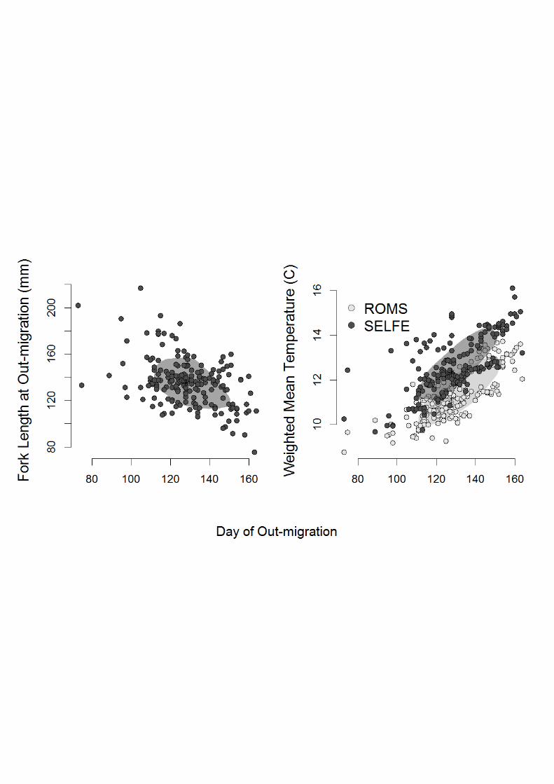
Temperature did not contribute substantially to estimates of swim speed, but this may have been because of its correlation with date and fish size. That is, temperature increased throughout the season, such that fish entering the ocean later, which tended to be smaller in size, experienced higher temperatures (Figure 6). Date of freshwater exit was a significant factor in determining swim speed; nevertheless, causal relationships are difficult to tease apart when covariate data are correlated. It is possible that temperature influenced swim speed mechanistically, but the model accounted for this effect via the day-of-year variable.

ConsumptionandgrowthratesdrivenbymigrationtimingandtemperatureWe found significant variability in consumption rate (g/g/d) both within and among years, but no difference in estimated consumption rate between stocks or oceanographic models. Based on the generalized linear model, several factors independently influenced estimated consumption rates (Figure 7). First, estimated means and variances increased with date of ocean entry, so fish entering the ocean later had higher consumption rates. Interestingly, consumption rates increased with ocean residence time, regardless of entry date, so both ocean entry timing and residence time influenced consumption rates.

In contrast to its contribution to estimates of swim speed, temperature was highly informative in accounting for consumption rates, with higher temperatures resulting in greater rates of consumption, despite the correlation between date and temperature. Higher rates of consumption were also estimated for fish captured at higher latitudes and those that experienced weak southward currents. Finally, all else being equal, small fish consumed more per unit body mass than large fish, as would be expected from an energetics standpoint.

We obtained similar results when evaluating simulations with respect to growth rate (mm/d) as we did for consumption rate. The one notable difference was that estimated growth rates were not significantly related to temperature.

Discussion

SwimspeedOur analysis clearly shows that interannual variation in coastal currents (e.g., Burla et al. 2010) results in altered yearling Chinook salmon migration behavior. If salmon possess a "map sense" or the ability to know their ocean location (Putman et al. 2013, Burke et al. 2014, Putman et al. 2014), then our results suggest they use that sense in altering swim speed and angle to counteract the effects of coastal currents.

When simulated fish encountered strong southerly flows, they compensated by increasing northward swim speed. Similarly, when northwest winds drove offshore surface currents, fish

11

responded by altering their swim angle towards shore. These dynamic behavioral responses would be required to maintain the surprisingly consistent spatial distributions observed for these stocks over the years (Peterson et al. 2010, Weitkamp 2010, Teel et al. 2015). Therefore, we inferred that for yearling Chinook salmon, migration behavior, as well as rates of consumption and growth at the individual level, are influenced by interannual variation in ocean currents.

Ample evidence supports the concept that timing of the juvenile migration plays a large role in determining marine survival (Scheuerell et al. 2009, Chittenden et al. 2010, McMichael et al. 2013), and our results provide insight into the underlying mechanisms of this concept. Juvenile fish that migrate early tend to be larger, which may by itself result in higher rates of survival due to size-selective mortality (Zabel and Williams 2002, Duffy and Beauchamp 2011, Woodson et al. 2013). Our model clearly demonstrated a time-dependent aspect to migration behavior, with swim speeds increasing throughout spring and summer. Tomaro et al. (2012) and Miller et al. (2014) also found an increase in movement rates with date, but their analyses did not account for ocean currents. We estimated swim speeds between 35 and 220% higher than those previously estimated because of the counteracting effect of southward currents. Whether or not individual fish increase swim speed through time, or whether late migrants have higher (but constant) swim speeds than early migrants, are questions not clarified by any of these analyses, including ours.

Most estimates of marine migration rate are based on average travel time between two points of detection (e.g., Thorstad et al. 2007, Welch et al. 2011). While these estimates have greatly increased our understanding of migration behavior, questions about the realized migration length or energetic expenditure of a migrating animal have remained unanswered. Simulated fish in our models swam 3 to 4 times farther than indicated by the net displacement between detection points, suggesting that the impact of ocean currents on salmon swim speed can be substantial. This is particularly relevant when considering migration energetics, since swim speed is a major component of the fish's energetic budget (Brett 1995, Brown et al. 2006). For this reason, an assumption of straight-line movement that ignores the influence of ocean currents can lead to dramatic bias in our understanding of physiology, movement, and behavior (Gaspar et al. 2006).

Early-migrating fish swam slower and experienced lower temperatures than later migrating fish (Figures 5 and 6), both of which can contributed to lower metabolic rates. They also had lower consumption rates. Thus, despite the fact that early migrants had slightly lower growth rates, their growth efficiency (growth/consumption) was consistent with that of later migrants. This suggests that the reduced growth observed in early migrants was related more to lower consumption rates than to colder temperatures. Unfortunately, this modeling exercise could not inform the cause of lower consumption rates for early migrants.

In most shallow freshwater environments, fish have a visual reference for movement relative to the substrate. By contrast, during the ocean migration, juvenile salmon in particular must reference their movement relative to some other aspect of the environment (Lohmann et al. 2008,

12

Putman et al. 2014). For salmon and other marine-migrating species, movement must be referenced using stimuli such as temperature, food resources, or the geomagnetic field.

Therefore, when alongshore currents intensify or winds shift and alter the trajectory of surface currents, surface-oriented fish such as juvenile salmon must either detect these changes directly or sense the changes in their position relative to external cues (Chapman et al. 2011). Recent evidence from tagging studies imply the latter, where fish are temporarily advected by strong currents and adjust behavior as a response (McMichael et al. 2013).

Although our study did not consider sensory modalities used by fish during migration, our models suggest that fish respond to shifts in the environment with dynamic behavior, and that these behavioral adjustments can be stock-specific. Indeed, stock-specific responses to the environment may have driven the seasonal shifts towards shore that have been observed previously in the stocks considered here (Teel et al. 2015).

Accuracy in our results was dependent on the accuracy of both the hydrodynamic models and the otolith analyses used for model inputs. Although we did not perform a thorough sensitivity analyses, our results showed clearly that errors in these components could propagate through the model and bias our results. Nevertheless, we were able to characterize which results were most sensitive to potential bias by using two oceanographic models. For example, temperature and ocean currents experienced by simulated fish were highly dependent on the ocean model used; estimated swim speeds also varied by ocean model. As these types of coupled oceanographic and individual-based models have recently seen widespread use (Byron and Burke 2014), we advise conservative interpretation of direct model outputs.

However, comparisons of relative swim speed between stocks, or between groups such as early vs. late migrants, were less sensitive to the choice of model and appeared more robust than absolute measures of behavior or movement. Where feasible, we suggest incorporating these relative comparisons directly into the research design to allow more confidence in model results.

Several aspects of behavior were intentionally left out of the model for simplicity. We did not include a dynamic swim speed, although we believe such a mechanism is likely. We also did not model diel variation in swim speed for simulated fish. Therefore, mean simulated swim speed may be biased if there is a diel pattern, with more active swimming during the day (Krutzikowsky and Emmett 2005).

Similarly, although the model was three–dimensional, and ocean currents affected simulated fish depth, we did not model vertical movement behavior (i.e., vertical movement was assumed to be passive). However, all simulated fish remained in the upper 30 m or so, which is within the observed depth range for the majority of juvenile salmon in the ocean (Emmett et al. 2004). Furthermore, to characterize the partitioning of time spent by fish in behaviors such as directed northward migration, random foraging, and diel vertical movement, would require movement

13

information on a finer scale than is currently available for the oceanic migration of juvenile salmon.

ConsumptionandgrowthratesOne of the reasons salmon migrate to the ocean is the potential for fast growth (Healey 1991). However, temporal dynamics dictate how this growth may be achieved. We suggest that the positive correlation between coastal ocean residence time and growth involves three possible mechanisms.

First, the correlation may be due to a lag effect between increased feeding and somatic growth, wherein fish that have arrived in the ocean more recently have had insufficient time for somatic growth to be realized. Second, it could be the result of an ontogenetic shift in primary diet from invertebrates to fish, which occurs at about the time salmon begin the juvenile marine migration (Daly et al. 2009). Correspondingly, longer coastal residence times would increase the probability that the salmon will reach a size that allows piscivorous foraging, which provides higher energetic returns and further enhances growth in a self-reinforcing manner. Finally, the correlation may be related to seasonal trends in prey availability. If juvenile salmon migrate too early, they may arrive before large numbers of prey are available, which may explain why the earliest migrants had the lowest consumption rates (Figure 7).

Fiechter et al. (2015) estimated that early-migrating Chinook salmon from San Francisco Bay had low growth during their first 90 days at sea, relative to later migrants. However, for early migrants, longer residence in the high-reward marine habitat more than compensated for their low early growth. Correspondingly, the early migrants were substantially larger by the end of the summer than the later migrants. We found similar results in Columbia River Chinook, for which early migrants had lower consumption and growth rates but enjoyed longer periods of marine growth.

However, in our study, early migrants entered the ocean at a larger size than later migrants. Thus, we could make no general inferences about the costs vs. benefits of early migration. Most likely, there is an optimal timing for migration that varies annually depending on factors such as growth response of the forage base to the timing of peak primary productivity and the characteristics of organisms transported into coastal waters.

For simplicity, our simulations used a constant energetic density for prey organisms. In reality, food quality shifts seasonally (Daly et al. 2009) and annually (Brodeur et al. 2007). It is possible that differences in estimated consumption were due to differences in the relative abundance of high-quality food in the diet among months and years. Prey quality is particularly influential in bioenergetics models (Beauchamp et al. 1989) and could have large impacts on results; therefore, results from our bioenergetics modeling should be viewed with caution. Nevertheless we cannot understate the importance of a bioenergetics submodel in this type of individual-based model.

14

Many aspects of behavior are size-dependent; having fish grow at realistic rates throughout a simulation can dramatically influence movement rates, and thus how we characterize behavior.

ConclusionsOur analysis has demonstrated how better estimates of swim speed, movement paths, and stock-specific migration dynamics may be obtained by accounting for the effects of ocean currents on salmon migration behavior. To maintain a relatively northward migration along the coast, migrating salmon must adjust their swimming to counteract seasonal and daily variations in coastal currents. As the season progressed, estimated swim speeds and consumption rates both increased, suggesting that the experiences and response to conditions of fish migrating later in the season differed from those of earlier migrants. These findings highlight the importance of phenology for migrating species (Anderson et al. 2013, Weitkamp et al. 2015).

While these analyses were not designed to directly address particular management issues, our results can provide insight as to how management strategies might affect ocean migration. For example, the timing of ocean entry significantly affects the conditions experienced by fish. Management actions such as hatchery release timing or barging juvenile salmon can affect ocean entry timing; therefore, such actions have a high likelihood of impacting the behavior and experiences of salmon during their northward marine migration.

Individual-based models have significantly contributed to our understanding of ecology (DeAngelis and Gross 1992, Grimm and Railsback 2005). In many individual-based models, emergent properties of populations (as more than a group of individuals) have provided useful information. In other applications, such as this effort, their usefulness stems from their ability to account for the complex and highly dynamic environment experienced by individuals.

This ability also allows the model to elucidate the potential effects of current and proposed management approaches on salmon ocean ecology. For example, an existing management action to minimize mortality during downstream migration in the Columbia River is to barge juvenile salmon past multiple hydroelectric dams (McMichael et al. 2011, Sandford et al. 2012). Fish that are barged arrive in the estuary days to weeks earlier than fish migrating in the river, with unknown impacts on their physiology and ecology. By simulating these fish, one could estimate the physical, and at least some of the biological, conditions experienced by fish arriving in the ocean early vs those arriving later, and possibly suggest refinements to the timing or magnitude of barging.

Future modeling efforts should focus on 1) incorporating as much prey information as possible along with one or more agents of mortality, given the availability of these data, 2) combining behaviors and/or allowing spatially or temporally explicit behavior, as results suggested here, and 3) simulating more years and additional species or stocks of salmon. Variability in spatial distribution among stocks is substantial (Weitkamp 2010, Tucker et al. 2012, Teel et al. 2015),

15

and the behavioral differences that create this variability can help us to better understand the forces driving marine migration.

Acknowledgements Chinook salmon catch data were obtained during a survey funded by the Bonneville Power Administration and NOAA Fisheries. Parker MacCready conducted the ROMS model simulation used here and graciously provided the output. Many people assisted with the project organization and data collection, including Ed Casillas, Bill Peterson, Ric Brodeur, Bob Emmett, Kym Jacobson, Cheryl Morgan, Jen Zamon, Brian Beckman, Laurie Weitkamp, Don Van Doornik, David Kuligowski, Tom Wainwright, Joe Fisher, Susan Hinton, and Cindy Bucher. We thank Lisa Crozier, Eric Buhle, James Faulkner, and Mark Scheuerell for helpful discussions related to data analysis. Steve Smith, David Huff, Beth Sanderson, and JoAnne Butzerin provided useful comments on earlier drafts of this manuscript.

16

Tables

Table 1. Chinook salmon catch by year, month, and stock.

Chinook salmon catch Mid & Upper Columbia River Snake River May June May June Total 2003 - 25 9 9 43 2004 7 - 5 2 14 2006 15 9 6 6 36 2007 26 - 15 4 45 2008 25 - 6 20 51 Total 73 34 41 41 189

Table 2. Mean swim speed (BL/s) for Chinook salmon caught in May vs. June (one standard deviation in parentheses). A weighted mean swim speed was estimated for each of the 10,000 simulated fish and these were then averaged.

Chinook salmon swim speed Mid & Upper Columbia River Snake River May June May June 2003 1.1 (0.64) 1.16 (0.47) 1.1 (0.62) 2004 0.55 (0.4) 0.59 (0.47) 1.37 (0.95) 2006 0.58 (0.17) 0.59 (0.37) 0.57 (0.06) 0.52 (0.35) 2007 0.67 (0.41) 0.64 (0.33) 0.88 (0.48) 2008 0.6 (0.27) 0.6 (0.25) 1.05 (0.73)

17

Table 3. Output from generalized linear model of fish swim speed after model averaging using AIC.

Estimate Std. Error Variable Importance

(Intercept) -16.42 0.94 Capture month (June) -0.43 0.10 0.98 DOY (freshwater exit) 0.01 0.003 0.98 Initial fork length -0.005 0.001 1.00 Latitude of capture 0.34 0.02 1.00 Ocean model (SELFE) -0.18 0.04 1.00 Stock (Snake) -0.05 0.03 0.83 Swim Angle 0.005 0.002 0.79 Experienced east-west current strength 0.10 0.02 1.00 Experienced north-south current strength -0.27 0.01 1.00 Year 2004 -0.06 0.06

1.00 Year 2006 -0.29 0.07 Year 2007 -0.21 0.06 Year 2008 -0.17 0.06 Capture month (June) : Year 2004 0.18 0.08

0.97 Capture month (June) : Year 2006 0.18 0.09 Capture month (June) : Year 2007 0.38 0.10 Capture month (June) : Year 2008 0.23 0.07 Experienced current strength (east-west and north-south interaction) 0.03 0.01 0.98

Consumption -0.02 0.01 0.47 Brackish/Ocean residence time (days) -0.003 0.004 0.30 Ocean model by stock interaction 0.01 0.04 0.21 Temperature experienced 0.005 0.03 0.25

18

Figures

Fig. 1 Initial fish distribution for fish caught in May and June for all years combined. Snake River spring-summer Chinook salmon are represented by triangles and Mid & Upper Columbia River Chinook salmon are represented by circles. Spatial distributions do not necessarily represent CPUE from the trawl survey, but rather the subset for which we had corresponding otolith information. Size of the circle represent the days since freshwater exit.

Fig. 2 Location of oceanographic model nodes for both the SELFE and ROMS models.

Fig. 3 Frequency distribution of estimated swim speeds for the 189 real fish. Results are shown for both the ROMS and SELFE oceanographic models.

Fig. 4 Swim speed versus the north-south component of flow experienced by each fish (top) and swim angle versus the east-west component of flow (bottom). Polygons include the 50% of the data closest to the bivariate median for each of the oceanographic models used.

Fig. 5 Swim speed vs. back-calculated fish length at the time of freshwater exit (upper panel) and estimated day of out-migration (lower panel). Polygons include the 50th percentile of data closest to the bivariate median for each oceanographic model used.

Fig. 6 Relationship between back-calculated fork length at time of freshwater exit vs. day of out-migration (left) and weighted mean temperature experienced vs. day of out-migration (right). Shaded areas include the 50th percentile of the data closest to the bivariate median. As the left panel is not dependent on the oceanographic model, only one data set is shown.

Fig. 7 Estimated consumption rate (grams of prey per gram body mass per day) versus day of out-migration and temperature. Polygons include the 50% of the data closest to the bivariate median.

19

References

Anderson, J. J., E. Gurarie, C. Bracis, B. J. Burke, and K. L. Laidre. 2013. Modeling climate change impacts on phenology and population dynamics of migratory marine species. Ecological Modelling 264:83-97.

Baptista, A., B. Howe, J. Freire, D. Maier, and C. T. Silva. 2008. Scientific exploration in the era of ocean observatories. Computing in Science & Engineering 10:53-58.

Beauchamp, D. A., D. J. Stewart, and G. L. Thomas. 1989. Corroboration of a bioenergetics model for sockeye salmon. Transactions of the American Fisheries Society 118:597-607.

Brett, J. R. 1995. Energetics.in C. Groot, L. Margolis, and W. C. Clarke, editors. Physiological Ecology of Pacific Salmon. UBC Press, Vancouver, British Columbia.

Brodeur, R. D., E. A. Daly, C. E. Benkwitt, C. A. Morgan, and R. L. Emmett. 2011. Catching the prey: Sampling juvenile fish and invertebrate prey fields of juvenile coho and Chinook salmon during their early marine residence. Fisheries Research 108:65-73.

Brodeur, R. D., E. A. Daly, R. A. Schabetsberger, and K. L. Mier. 2007. Interannual and interdecadal variability in juvenile coho salmon (Oncorhynchus kisutch) diets in relation to environmental changes in the northern California Current. Fisheries Oceanography 16:395-408.

Brown, R., D. Geist, and M. Mesa. 2006. Use of Electromyogram Telemetry to Assess Swimming Activity of Adult Spring Chinook Salmon Migrating Past a Columbia River Dam. Transactions of the American Fisheries Society 135:281-287.

Burke, B. J., J. J. Anderson, and A. M. Baptista. 2014. Evidence for multiple navigational sensory capabilities of Chinook salmon. Aquatic Biology 20:77-90.

Burla, M., A. M. Baptista, Y. L. Zhang, and S. Frolov. 2010. Seasonal and interannual variability of the Columbia River plume: A perspective enabled by multiyear simulation databases. Journal of Geophysical Research-Oceans 115: C00B16.

Burnham, K. P. and D. R. Anderson. 2010. Model Selection and Multi-Model Inference: A Practical Information-Theoretic Approach. Springer.

Byron, C. J. and B. J. Burke. 2014. Salmon ocean migration models suggest a variety of population-specific strategies. Reviews in Fish Biology and Fisheries 24:737-756.

Chapman, J. W., R. H. Klaassen, V. A. Drake, S. Fossette, G. C. Hays, J. D. Metcalfe, A. M. Reynolds, D. R. Reynolds, and T. Alerstam. 2011. Animal orientation strategies for movement in flows. Current Biology 21:R861-870.

Chittenden, C. M., J. L. A. Jensen, D. Ewart, S. Anderson, S. Balfry, E. Downey, A. Eaves, S. Saksida, B. Smith, S. Vincent, D. Welch, and R. S. McKinley. 2010. Recent Salmon Declines: A Result of Lost Feeding Opportunities Due to Bad Timing? PLoS One 5.

CMOP. 2013. Virtual Columbia River. Page Interactive database available from http://www.stccmop.org/datamart/virtualcolumbiariver/simulationdatabases (accessed April 2013). Center for Marine and Coastal Observation & Prediction.

Cooke, S. J., S. G. Hinch, M. Wikelski, R. D. Andrews, L. J. Kuchel, T. G. Wolcott, and P. J. Butler. 2004. Biotelemetry: a mechanistic approach to ecology. Trends Ecol Evol 19:334-343.

Daly, E., R. Brodeur, and L. Weitkamp. 2009. Ontogenetic Shifts in Diets of Juvenile and Subadult Coho and Chinook Salmon in Coastal Marine Waters: Important for Marine Survival? Transactions of the American Fisheries Society 138:1420-1438.

20

Davis, K. A., N. S. Banas, S. N. Giddings, S. A. Siedlecki, P. MacCready, E. J. Lessard, R. M. Kudela, and B. M. Hickey. 2014. Estuary-enhanced upwelling of marine nutrients fuels coastal productivity in the U.S. Pacific Northwest. Journal of Geophysical Research-Oceans 119:8778-8799.

DeAngelis, D. L. and L. J. Gross. 1992. Individual-based Models and Approaches in Ecology: Populations, Communities, and Ecosystems. Chapman & Hall.

Duffy, E. J. and D. A. Beauchamp. 2011. Rapid growth in the early marine period improves the marine survival of Chinook salmon (Oncorhynchus tshawytscha) in Puget Sound, Washington. Canadian Journal of Fisheries and Aquatic Sciences 68:232-240.

Emmett, R. L., P. J. Bentley, and G. K. Krutzikowsky. 2001. Ecology of Marine Predatory and Prey Fishes off the Columbia River, 1998 and 1999.in D. o. Commerce, editor. NOAA Fisheries, Seattle, WA.

Emmett, R. L., R. D. Brodeur, and P. M. Orton. 2004. The vertical distribution of juvenile salmon (Oncorhynchus spp.) and associated fishes in the Columbia River plume. Fisheries Oceanography 13:392-402.

Fiechter, J., D. D. Huff, B. T. Martin, D. W. Jackson, C. A. Edwards, K. A. Rose, E. N. Curchitser, K. S. Hedstrom, S. T. Lindley, and B. K. Wells. 2015. Environmental conditions impacting juvenile Chinook salmon growth off central California: An ecosystem model analysis. Geophysical Research Letters:n/a-n/a.

Fisher, J. P., L. A. Weitkamp, D. J. Teel, S. A. Hinton, J. A. Orsi, E. V. Farley Jr., J. F. T. Morris, M. E. Thiess, R. M. Sweeting, and M. Trudel. 2014. Early Ocean Dispersal Patterns of Columbia River Chinook and Coho Salmon. Transactions of the American Fisheries Society 143:252-272.

Gaspar, P., J. Y. Georges, S. Fossette, A. Lenoble, S. Ferraroli, and Y. Le Maho. 2006. Marine animal behaviour: neglecting ocean currents can lead us up the wrong track. Proceedings of the Royal Society B-Biological Sciences 273:2697-2702.

Giddings, S. N., P. MacCready, B. M. Hickey, N. S. Banas, K. A. Davis, S. A. Siedlecki, V. L. Trainer, R. M. Kudela, N. A. Pelland, and T. P. Connolly. 2014. Hindcasts of potential harmful algal bloom transport pathways on the Pacific Northwest coast. Journal of Geophysical Research-Oceans 119:2439-2461.

Grimm, V. and S. F. Railsback. 2005. Individual-based Modeling And Ecology. Princeton University Press.

Haidvogel, D. B., H. G. Arango, K. Hedstrom, A. Beckmann, P. Malanotte-Rizzoli, and A. F. Shchepetkin. 2000. Model evaluation experiments in the North Atlantic Basin: simulations in nonlinear terrain-following coordinates. Dynamics of Atmospheres and Oceans 32:239-281.

Hanson, P., T. Johnson, D. Schindler, and J. Kitchell. 1997. Fish bioenergetics 3.0. University of Wisconsin, Sea Grant Institute. Center for Limnology.

Healey, M. C. 1991. Life history of Chinook salmon (Oncorhynchus tshawytscha).in C. Groot and L. Margolis, editors. Pacific salmon life histories. University of British Columbia Press, Vancouver, BC

Hewett, S. W. and B. L. Johnson. 1992. Fish bioenergetics model 2. University of Wisconsin, Sea Grant Institute, Madison, WI.

Hussey, N. E., S. T. Kessel, K. Aarestrup, S. J. Cooke, P. D. Cowley, A. T. Fisk, R. G. Harcourt, K. N. Holland, S. J. Iverson, J. F. Kocik, J. E. Mills Flemming, and F. G. Whoriskey.

21

2015. Aquatic animal telemetry: A panoramic window into the underwater world. Science 348:1255642.

Jacobson, K., B. Peterson, M. Trudel, J. Ferguson, C. Morgan, D. Welch, A. Baptista, B. Beckman, R. Brodeur, E. Casillas, R. Emmett, J. Miller, D. Teel, T. Wainwright, L. Weitkamp, J. Zamon, and K. Fresh. 2012. The Marine Ecology of Juvenile Columbia River Basin Salmonids: A Synthesis of Research 1998-2011. Northwest Power and Conservation Council.

Kalinowski, S. T., K. R. Manlove, and M. L. Taper. 2007. ONCOR a computer program for genetic stock identification. www.montana.edu/kalinowski/Software/ONCOR. html.

Kent, A. J. R. and C. A. A. Ungerer. 2006. Analysis of light lithophile elements (Li, Be, B) by laser ablation ICP-MS: Comparison between magnetic sector and quadrupole ICP-MS. American Mineralogist 91:1401-1411.

Krutzikowsky, G. and R. Emmett. 2005. Diel differences in surface trawl fish catches off Oregon and Washington. Fisheries Research 71:365-371.

Lohmann, K. J., C. M. Lohmann, and C. S. Endres. 2008. The sensory ecology of ocean navigation. Journal of Experimental Biology 211:1719-1728.

Matala, A. P., J. E. Hess, and S. R. Narum. 2011. Resolving adaptive and demographic divergence among Chinook salmon populations in the Columbia River Basin. Transactions of the American Fisheries Society 140:783-807.

McMichael, G. A., A. C. Hanson, R. A. Harnish, and D. M. Trott. 2013. Juvenile salmonid migratory behavior at the mouth of the Columbia River and within the plume. Animal Biotelemetry:1-14.

McMichael, G. A., J. R. Skalski, and K. A. Deters. 2011. Survival of Juvenile Chinook Salmon during Barge Transport. North American Journal of Fisheries Management 31:1187-1196.

Miller, J. A. 2009. The effects of temperature and water concentration on the otolith incorporation of barium and manganese in black rockfish Sebastes melanops. J Fish Biol 75:39-60.

Miller, J. A., V. L. Butler, C. A. Simenstad, D. H. Backus, A. J. R. Kent, and B. Gillanders. 2011. Life history variation in upper Columbia River Chinook salmon (Oncorhynchus tshawytscha): a comparison using modern and ~500-year-old archaeological otoliths. Canadian Journal of Fisheries and Aquatic Sciences 68:603-617.

Miller, J. A., A. Gray, and J. Merz. 2010. Quantifying the contribution of juvenile migratory phenotypes in a population of Chinook salmon Oncorhynchus tshawytscha. Marine Ecology Progress Series 408:227-240.

Miller, J. A., D. J. Teel, A. Baptista, C. A. Morgan, and M. Bradford. 2013. Disentangling bottom-up and top-down effects on survival during early ocean residence in a population of Chinook salmon (Oncorhynchus tshawytscha). Canadian Journal of Fisheries and Aquatic Sciences 70:617-629.

Miller, J. A., D. J. Teel, W. T. Peterson, and A. M. Baptista. 2014. Assessing the relative importance of local and regional processes on the survival of a threatened salmon population. PLoS One 9:e99814.

Neilson, J. D. and G. H. Geen. 1982. Otoliths of Chinook Salmon (Oncorhynchus tshawytscha) - Daily Growth Increments and Factors Influencing Their Production. Canadian Journal of Fisheries and Aquatic Sciences 39:1340-1347.

22

NOAA. 1992. Endandered and threatened species: threatened status for Snake River spring/summer Chinook salmon.in N. O. a. A. Administration, editor. Federal Register 57(78). National Oceanic and Atmoshperic Administration.

Peterson, W. T., C. A. Morgan, J. P. Fisher, and E. Casillas. 2010. Ocean distribution and habitat associations of yearling coho (Oncorhynchus kisutch) and Chinook (O. tshawytscha) salmon in the northern California Current. Fisheries Oceanography 19:508-525.

Putman, N. F., K. J. Lohmann, E. M. Putman, T. P. Quinn, A. P. Klimley, and D. L. Noakes. 2013. Evidence for geomagnetic imprinting as a homing mechanism in Pacific salmon. Current Biology 23:312-316.

Putman, N. F., M. M. Scanlan, E. J. Billman, J. P. O'Neil, R. B. Couture, T. P. Quinn, K. J. Lohmann, and D. L. Noakes. 2014. An inherited magnetic map guides ocean navigation in juvenile Pacific salmon. Current Biology 24:446-450.

Ruzicka, J. J., R. D. Brodeur, R. L. Emmett, J. H. Steele, J. E. Zamon, C. A. Morgan, A. C. Thomas, and T. C. Wainwright. 2012. Interannual variability in the Northern California Current food web structure: Changes in energy flow pathways and the role of forage fish, euphausiids, and jellyfish. Progress In Oceanography 102:19-41.

Sandford, B. P., R. W. Zabel, L. G. Gilbreath, and S. G. Smith. 2012. Exploring Latent Mortality of Juvenile Salmonids Related to Migration through the Columbia River Hydropower System. Transactions of the American Fisheries Society 141:343-352.

Scheuerell, M. D., R. W. Zabel, and B. P. Sandford. 2009. Relating juvenile migration timing and survival to adulthood in two species of threatened Pacific salmon (Oncorhynchus spp.). Journal of Applied Ecology 46:983-990.

Seeb, L. W., A. Antonovich, A. A. Banks, T. D. Beacham, A. R. Bellinger, S. M. Blankenship, A. R. Campbell, N. A. Decovich, J. C. Garza, C. M. Guthrie, T. A. Lundrigan, P. Moran, S. R. Narum, J. J. Stephenson, K. J. Supernault, D. J. Teel, W. D. Templin, J. K. Wenburg, S. E. Young, and C. T. Smith. 2007. Development of a standardized DNA database for Chinook salmon. Fisheries 32:540-552.

Siedlecki, S. A., N. S. Banas, K. A. Davis, S. Giddings, B. M. Hickey, P. MacCready, T. Connolly, and S. Geier. 2015. Seasonal and interannual oxygen variability on the Washington and Oregon continental shelves. Journal of Geophysical Research-Oceans 120:608-633.

Sutherland, D. A., P. MacCready, N. S. Banas, and L. F. Smedstad. 2011. A Model Study of the Salish Sea Estuarine Circulation. Journal of Physical Oceanography 41:1125-1143.

Teel, D. J., B. J. Burke, D. R. Kuligowski, C. A. Morgan, and D. M. Van Doornik. 2015. Genetic Identification of Chinook Salmon: Stock-Specific Distributions of Juveniles along the Washington and Oregon Coasts. Marine and Coastal Fisheries 7:274-300.

Thorstad, E., F. Økland, B. Finstad, R. Sivertsgård, N. Plantalech, P. Bjørn, and R. S. McKinley. 2007. Fjord migration and survival of wild and hatchery-reared Atlantic salmon and wild brown trout post-smolts. Hydrobiologia 582:99-107.

Tomaro, L. M., D. J. Teel, W. T. Peterson, and J. A. Miller. 2012. When is bigger better? Early marine residence of middle and upper Columbia River spring Chinook salmon. Marine Ecology Progress Series 452:237-252.

Tucker, S., M. Trudel, D. W. Welch, J. R. Candy, J. F. T. Morris, M. E. Thiess, C. Wallace, and T. D. Beacham. 2012. Annual coastal migration of juvenile Chinook salmon: static stock-specific patterns in a highly dynamic ocean. Marine Ecology Progress Series 449:245-262.

23

Waples, R. S., D. J. Teel, J. M. Myers, and A. R. Marshall. 2004. Life-history divergence in Chinook salmon: Historic contingency and parallel evolution. Evolution 58:386-403.

Weitkamp, L. 2010. Marine distributions of Chinook salmon from the west coast of North America determined by coded wire tag recoveries. Transactions of the American Fisheries Society 139:147-170.

Weitkamp, L. A., D. J. Teel, M. Liermann, S. A. Hinton, D. M. Van Doornik, and P. J. Bentley. 2015. Stock-Specific Size and Timing at Ocean Entry of Columbia River Juvenile Chinook Salmon and Steelhead: Implications for Early Ocean Growth. Marine and Coastal Fisheries 7:370-392.

Welch, D. W., M. C. Melnychuk, J. C. Payne, E. L. Rechisky, A. D. Porter, G. D. Jackson, B. R. Ward, S. P. Vincent, C. C. Wood, and J. Semmens. 2011. In situ measurement of coastal ocean movements and survival of juvenile Pacific salmon. Proceedings of the National Academy of Sciences of the United States of America 108:8708-8713.

Welch, D. W., M. C. Melnychuk, E. R. Rechisky, A. D. Porter, M. C. Jacobs, A. Ladouceur, R. S. McKinley, and G. D. Jackson. 2009. Freshwater and marine migration and survival of endangered Cultus Lake sockeye salmon (Oncorhynchus nerka) smolts using POST, a large-scale acoustic telemetry array. Canadian Journal of Fisheries and Aquatic Sciences 66:736-750.

Woodson, L. E., B. K. Wells, P. K. Weber, R. B. MacFarlane, G. E. Whitman, and R. C. Johnson. 2013. Size, growth, and origin-dependent mortality of juvenile Chinook salmon Oncorhynchus tshawytscha during early ocean residence. Marine Ecology Progress Series 487:163-175.

Zabel, R. W. and J. G. Williams. 2002. Selective mortality in chinook salmon: What is the role of human disturbance? Ecological Applications 12:173-183.