estimating head orientation with stereo vision
TRANSCRIPT

Estimating Head Orientation
with Stereo Vision
Diplomarbeit
Edgar Seemann
Interactive Systems Labs
Universitat Karlsruhe (TH)
Advisors:
Prof. Dr. Alex WaibelDr.-Ing. Rainer Stiefelhagen
November 27, 2003

Hiermit versichere ich, die vorliegende Diplomarbeit personlich und ohneunzulassige Hilfsmittel angefertigt zu haben. Alle verwendeten Quellen sindim Literaturverzeichnis aufgefuhrt.
Karlsruhe, 30. November 2003
Abstract
Interpretation of human behaviors in video data is essential for naturaland intuitive human-computer interfaces. In this context, the estimation of aperson’s head pose plays a major role, since heads and faces are continuouslyused in interaction between people.
In this work we present a method for estimating a person’s head posewith a stereo camera. Our approach focuses on the application of human-robot interaction, where people may be further away from the camera andmay move freely around in a room.
First, the 3D scene is reconstructed from the images of a stereo cameraby calculating depth information. Subsequently, the face is extracted witha color-based face tracking approach. Finally, the resulting 3D face modelis preprocessed by a number of normalization algorithms. The estimation isbased on neural networks, which are trained to compute the head pose fromgray scale and depth information.
We show that depth information not only helps improving the accuracyof the pose estimation, but also improves the robustness of the system whenthe lighting conditions change.
The system can handle pan and tilt rotations from −90◦ to +90◦ andachieves high accuracy in a realistic environment. It doesn’t require anymanual initialization and doesn’t suffer from drift during an image sequence.Moreover, the system is capable of real-time processing.

Acknowledgements
This work was conducted at the Interactive Systems Labs as part of mystudies at the Universitat Karlsruhe (TH). I would like to thank all membersof the laboratory for participating in the various data collections performedduring this work. I am particularly grateful for the help of Kai Nickel whowas always there for advice regarding the stereo camera and implementationdetails. Furthermore I thank my advisor Rainer Stiefelhagen for his constantsupport.

Contents
1 Introduction 41.1 Motivation . . . . . . . . . . . . . . . . . . . . . . . . . . . . . 41.2 Possible Applications . . . . . . . . . . . . . . . . . . . . . . . 51.3 Requirements for a Head Pose Estimation Technique . . . . . 61.4 Related Work . . . . . . . . . . . . . . . . . . . . . . . . . . . 7
1.4.1 Feature-Based Techniques . . . . . . . . . . . . . . . . 71.4.2 View-Based Techniques . . . . . . . . . . . . . . . . . . 81.4.3 Summary . . . . . . . . . . . . . . . . . . . . . . . . . 10
2 The Head Pose Tracking Technique 122.1 Overview . . . . . . . . . . . . . . . . . . . . . . . . . . . . . . 132.2 Stereo Vision . . . . . . . . . . . . . . . . . . . . . . . . . . . 14
2.2.1 Stereo Algorithm . . . . . . . . . . . . . . . . . . . . . 142.2.2 Finding Corresponding Pixels . . . . . . . . . . . . . . 152.2.3 Calculating Object Distance . . . . . . . . . . . . . . . 16
2.3 Face Detection and Extraction . . . . . . . . . . . . . . . . . . 182.3.1 Pattern-Based Vs. Color-Based Face Detection . . . . 182.3.2 Finding A Skin Color Region . . . . . . . . . . . . . . 202.3.3 Building The Color-Model . . . . . . . . . . . . . . . . 212.3.4 Face Extraction . . . . . . . . . . . . . . . . . . . . . . 22
2.4 Preprocessing . . . . . . . . . . . . . . . . . . . . . . . . . . . 272.4.1 Resizing 3D Face Model . . . . . . . . . . . . . . . . . 272.4.2 Downsampling . . . . . . . . . . . . . . . . . . . . . . 282.4.3 Depth normalization . . . . . . . . . . . . . . . . . . . 292.4.4 Gray Value Normalization . . . . . . . . . . . . . . . . 29
2.5 Estimating Head Pose With Neural Networks . . . . . . . . . 312.5.1 Neural Network Topology . . . . . . . . . . . . . . . . 312.5.2 Advantages Of This Approach . . . . . . . . . . . . . . 33
2

CONTENTS
3 Experimental Results 353.1 Data Collection “Portrait View” . . . . . . . . . . . . . . . . . 353.2 Experiments “Portrait View” . . . . . . . . . . . . . . . . . . 37
3.2.1 Test 1 - Known Users . . . . . . . . . . . . . . . . . . . 383.2.2 Test 2 - Unknown Users . . . . . . . . . . . . . . . . . 403.2.3 Test 3 - Changed Lighting Conditions . . . . . . . . . . 423.2.4 Error Analysis . . . . . . . . . . . . . . . . . . . . . . . 43
3.3 Data Collection “Robot Scenario” . . . . . . . . . . . . . . . . 453.4 Experiments “Robot Scenario” . . . . . . . . . . . . . . . . . . 46
3.4.1 Test 1 - Known Users . . . . . . . . . . . . . . . . . . . 473.4.2 Test 2 - Unknown Users . . . . . . . . . . . . . . . . . 493.4.3 Error Analysis . . . . . . . . . . . . . . . . . . . . . . . 503.4.4 Filtering . . . . . . . . . . . . . . . . . . . . . . . . . . 51
4 Head Pose Estimation in Applications 544.1 The Real-Time System . . . . . . . . . . . . . . . . . . . . . . 544.2 Tracking Of Pointing Gestures With The Help Of Head Ori-
entation . . . . . . . . . . . . . . . . . . . . . . . . . . . . . . 55
5 Conclusion and Future Work 58
A Neural Networks 60A.1 Introduction To Neural Networks . . . . . . . . . . . . . . . . 60A.2 Advantages Of Neural Networks . . . . . . . . . . . . . . . . . 60A.3 Building Blocks Of Neural Networks . . . . . . . . . . . . . . 61A.4 Learning With Neural Networks . . . . . . . . . . . . . . . . . 63
A.4.1 Linear Discriminant Functions and Single-Layer Net-works . . . . . . . . . . . . . . . . . . . . . . . . . . . 63
A.4.2 The Perceptron . . . . . . . . . . . . . . . . . . . . . . 65A.4.3 Multi-Layer Networks . . . . . . . . . . . . . . . . . . 66
A.5 Generalization Of Neural Networks . . . . . . . . . . . . . . . 70
B Pattern-Based Face Detection 72B.1 Learning Classification Functions . . . . . . . . . . . . . . . . 73
C Discrete Kalman Filter 76C.1 Basic Kalman Filter Equations . . . . . . . . . . . . . . . . . 77C.2 The Predictor-Corrector Process . . . . . . . . . . . . . . . . . 78
References 80
3

Chapter 1
Introduction
1.1 Motivation
Advancing human-robot interaction has been an active research field in re-cent years [Perz2001, Agah2001, Koku2000, Adam2000, Mats1999]. A majorchallenge is the tracking and interpretation of human behaviors in video data,since it is essential for enabling natural human-robot interaction.
In order to fully understand what a user does or intends to do, a robot shouldbe capable of detecting and understanding many of the communicative cuesused by humans. This involves in particular the recognition and interpre-tation of human faces. In interaction between people faces are continuouslyused to signal interest, emotion and direction of attention. Monitoring suchinformation therefore can be used to make interaction with a robot morenatural and intuitive.
Monitoring a person’s head orientation is an important step towards buildingbetter human-robot interfaces. Since head orientation is related to a person’sdirection of attention, it can give us useful information about the objects orpersons with which a user is interacting. It can furthermore be used to helpa robot decide whether he was addressed by a person or not [SYW2001].
While eye gaze certainly is another important cue for a person’s direction ofattention [Stie2002], in most realistic scenarios image resolution of a person’seyes isn’t sufficiently high to see the pupils or irises.
4

1.2 Possible Applications
Hence, in this work we propose a method for estimating a person’s head pose.Estimation is based on image pairs obtained from a stereo camera.
1.2 Possible Applications
We distinguish three main application areas for head pose estimation:
• Active control applications
• Passive understanding
• Applications for which head pose estimation is a prerequisite
In active control applications a user directly controls an interface with hishead pose. He can, for example, use it for pointing when hands are otherwiseengaged or as a complementary information when desired action has manyinput parameters. This is also of particular importance for users with dis-abilities. Another scenario in this area is car headlight control. If a driverperceives, for example, the silhouettes of pedestrians next to the road, chang-ing the focus of the headlights a little to the road border might help him tobetter see and avoid dangerous situations.
Passive understanding techniques might be used in dialog applications, wherethe computer tries to understand what is going on in a room, meeting etc. Itis, for example, interesting to know who is talking to whom during a meeting.In human-robot applications it is crucial to identify whether the user wastalking to the robot, another person or referring to a different object. Forall these applications the head pose gives an indication of the user’s focus ofattention and therefore helps to understand the context of the dialog.
Applications for which head pose estimation is a prerequisite include facerecognition and emotion detection. Knowing the head pose of a person helpsfinding facial features like eyes, nose, mouth etc. which might be usefulto determine a person’s identity. These facial features are also crucial foremotion detection. Since these are mostly expressed by the mimic.
In this work, the application we are particularly interested in is a human-robot interaction scenario. A robot should be able to detect the direction ofattention of a person in his field of view. In particular, the robot should be
5

1.3 Requirements for a Head Pose Estimation Technique
able to determine if a person is looking at him and execute speech commandsif he was addressed. Additionally, he should be able to process a user’spointing gestures, which he recognizes via the tracking of hands and thehead orientation.
1.3 Requirements for a Head Pose Estima-
tion Technique
Current head pose estimation techniques are still error-prone. They are gen-erally unable to accurately track large rotations under rapid illuminationvariation, which are common in interactive environments (and airplane orautomotive cockpits) [MRC2002].
On the other hand special head tracking hardware (like magnetic sensors)provides an accuracy which is sufficient for most applications. However thishardware is expensive and intrusive. Users often feel discomfort because thehardware restricts their natural motion.
In order to be feasible in practice a head pose estimation technique forhuman-robot interaction consequently has to satisfy certain criteria. Basedon [MA2000] we state these six criteria:
• Non-intrusive (no markers, magnetic sensors etc.)
• Passive
• Robust to occlusions, deformations and lighting fluctuations
• Accurate
• Able to track rotations from -90 to +90 degrees
• Capable of real-time processing
In this work we are proposing a technique which has been designed by takinginto account all of these six criteria.
Our focus is especially on robustness under different lighting conditions. Thisis an obstacle for current image-based techniques. Not only do the color
6
1.4 Related Work
values vary if there is artificial light or day light, but additionally the imageedges and shadows change if the position of the light source is altered.
This is one of the reasons why we propose a technique that uses stereo vision.Depth information is largely invariant to changing lighting conditions and cantherefore improve the result of head pose estimation.
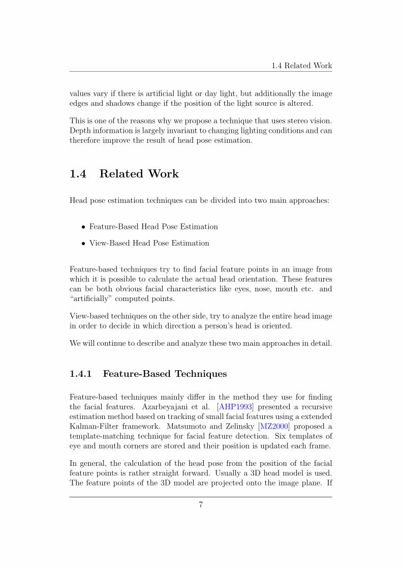
1.4 Related Work
Head pose estimation techniques can be divided into two main approaches:
• Feature-Based Head Pose Estimation
• View-Based Head Pose Estimation
Feature-based techniques try to find facial feature points in an image fromwhich it is possible to calculate the actual head orientation. These featurescan be both obvious facial characteristics like eyes, nose, mouth etc. and“artificially” computed points.
View-based techniques on the other side, try to analyze the entire head imagein order to decide in which direction a person’s head is oriented.
We will continue to describe and analyze these two main approaches in detail.
1.4.1 Feature-Based Techniques
Feature-based techniques mainly differ in the method they use for findingthe facial features. Azarbeyajani et al. [AHP1993] presented a recursiveestimation method based on tracking of small facial features using a extendedKalman-Filter framework. Matsumoto and Zelinsky [MZ2000] proposed atemplate-matching technique for facial feature detection. Six templates ofeye and mouth corners are stored and their position is updated each frame.
In general, the calculation of the head pose from the position of the facialfeature points is rather straight forward. Usually a 3D head model is used.The feature points of the 3D model are projected onto the image plane. If
7
1.4 Related Work
the orientation of the 3D model corresponds to the head orientation in theimage, the projected feature points must lie close to the found feature pointsin the image. Matsumoto and Zelinsky [MZ2000] are using stereo visionto calculate the head orientation. The projection onto the image plane istherefore not necessary any more. In this case the problem results in thecalculation of a rotation matrix R and a translation vector t which minimizethe squared fitting error E in the following equation:
E =N−1∑i=0
wi(Rxi + t− yi)T (Rxi + t− yi)
where N is the number of features, xi the coordinate of a feature in the 3Dmodel and yi the coordinate of a feature acquired via feature detection. wi isa weighting factor for each measurement. This problem can be solved usingleast squares.
Feature-based methods usually have the limitation that the same points mustbe visible over the entire image sequence, thus limiting the range of headmotions they can track [YZ2001]. For a human-robot application whereusers move freely in the room such a limitation is a serious drawback.
Another drawback of this approach is that robust detection of facial featuresis extremely difficult under unconstrained conditions and large variations inhead position. [SB2002]
1.4.2 View-Based Techniques
There is a wide range of view-based approaches for head pose estimation. Inthis section we want to introduce some of these and approaches and presentdifferent techniques they apply.
Template Matching
Template matching is probably the easiest and most straight forward ap-proaches. For each person and angle range a reference image is stored ina database. Captured images are afterwards compared to these referenceframes. The reference frame which has the most similarity to the image is
8
1.4 Related Work
selected as head pose. Since angle ranges of 30 degrees are common, thistechnique gives only a rough estimate of the head pose.
Ellipse Fitting
Ellipse fitting tries to align an ellipse with the outline of the head. The actualhead pose is subsequently estimated from the shape of this ellipse. Ellipsefitting is rather fast, but not very accurate.
Eigenspace-based
Srinivasan and Boyer [SB2002] proposed a head pose estimation techniqueusing view-based eigenspaces. They used principal component analysis tobuild seven eigenspaces for different angle ranges from example images. Anytest image x could afterwards be projected onto an eigenspace by evaluatingthe inner product of x with the eigenvectors yi. The norm of the resultingvector ci = xT yi gives the fraction of energy of the test image lying in theeigenspace. The eigenspace with the highest fraction of energy should finallycorrespond to the angle range of the test image.
Since head orientation can only be matched to one of the seven eigenspaces,this technique gives only a rough estimate of the actual head pose.
Optical Flow and Motion Detection
Optical-flow-based approaches try to estimate the velocity and direction withwhich a pixel has moved from one image to another. The relative motion ofan object can directly be calculated from these pixel velocities. Horn andSchunck [HS1980] have proposed a technique to calculate the optical flow inarbitrary image sequences efficiently. Morency et al. [MRC2002] applied thistechnique to head pose estimation and extended it for the use with stereoinformation.
However, calculating the relative head rotation from each image frame to thenext, causes an accumulation of the estimation error. This phenomenon iscalled drift and leads to a degrading performance on long image sequences.Another drawback of this technique is the fact that the initial head pose has
9

1.4 Related Work
to be known. Manual initialization is therefore required.
Neural-Network-based
Stiefelhagen et al. [SYW2001] proposed a neural network based approach forhead pose estimation in human-robot interaction. They normalize the his-togram of the face image and map it to neural network input units. Further-more they are retrieving image edges and feed them as additional informationinto the neural network.
This technique is accurate when lighting conditions do not change. Underchanging lighting conditions, however the performance degrades considerably.
1.4.3 Summary
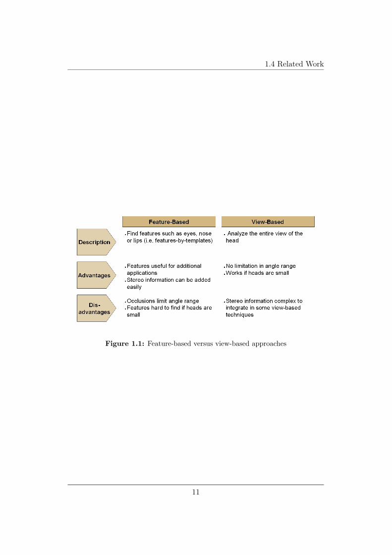
Feature-based approaches tend to be rather accurate. Moreover facial fea-tures can be used for additional applications like face recognition or emotiondetection. However, it is difficult to find facial feature points, especially whenheads in an image are small and camera resolution is not sufficiently high.
View-based approaches work also if heads are small. Furthermore they donot limit the angle range because of occlusions. The combination with stereovision, however, is sometimes complex.
Figure 1.1 shows a quick overview of the two main approaches.
10
1.4 Related Work
Figure 1.1: Feature-based versus view-based approaches
11
Chapter 2
The Head Pose TrackingTechnique
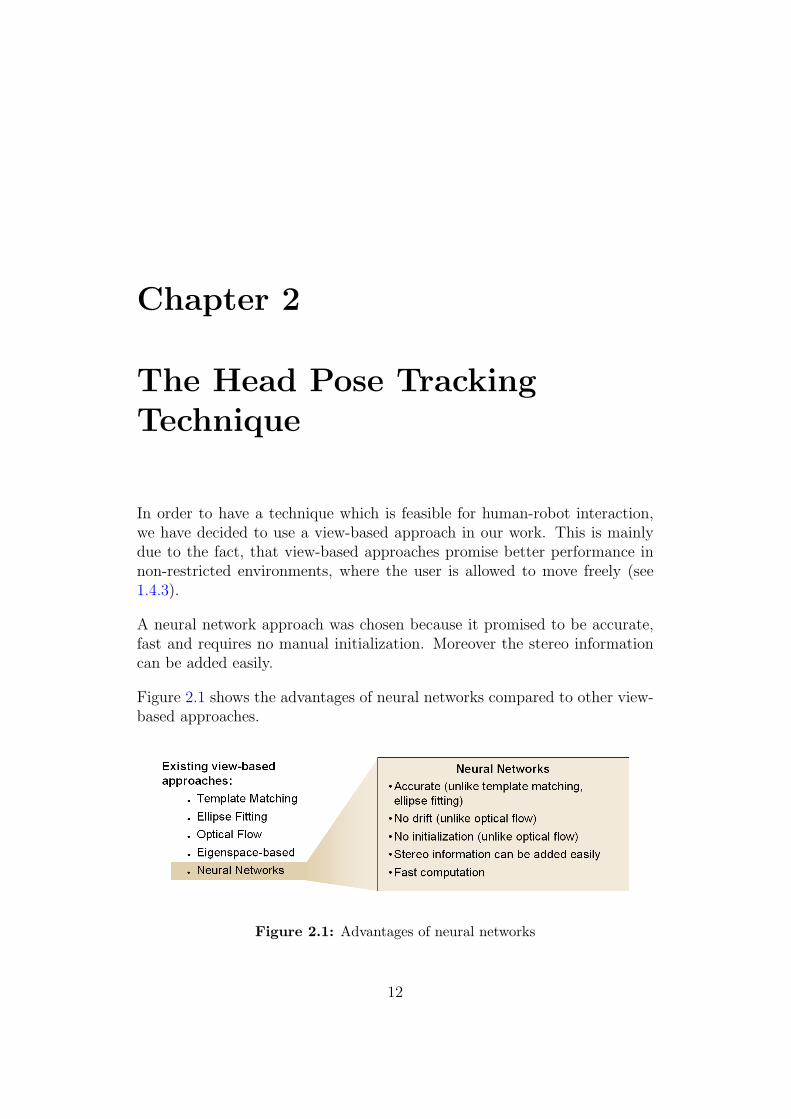
In order to have a technique which is feasible for human-robot interaction,we have decided to use a view-based approach in our work. This is mainlydue to the fact, that view-based approaches promise better performance innon-restricted environments, where the user is allowed to move freely (see1.4.3).
A neural network approach was chosen because it promised to be accurate,fast and requires no manual initialization. Moreover the stereo informationcan be added easily.
Figure 2.1 shows the advantages of neural networks compared to other view-based approaches.
Figure 2.1: Advantages of neural networks
12
2.1 Overview
2.1 Overview
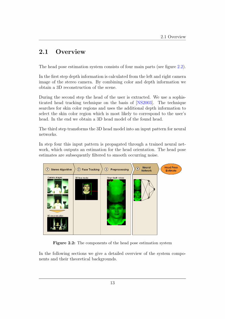
The head pose estimation system consists of four main parts (see figure 2.2).
In the first step depth information is calculated from the left and right cameraimage of the stereo camera. By combining color and depth information weobtain a 3D reconstruction of the scene.
During the second step the head of the user is extracted. We use a sophis-ticated head tracking technique on the basis of [NS2003]. The techniquesearches for skin color regions and uses the additional depth information toselect the skin color region which is most likely to correspond to the user’shead. In the end we obtain a 3D head model of the found head.
The third step transforms the 3D head model into an input pattern for neuralnetworks.
In step four this input pattern is propagated through a trained neural net-work, which outputs an estimation for the head orientation. The head poseestimates are subsequently filtered to smooth occurring noise.
Figure 2.2: The components of the head pose estimation system
In the following sections we give a detailed overview of the system compo-nents and their theoretical backgrounds.
13
2.2 Stereo Vision
2.2 Stereo Vision
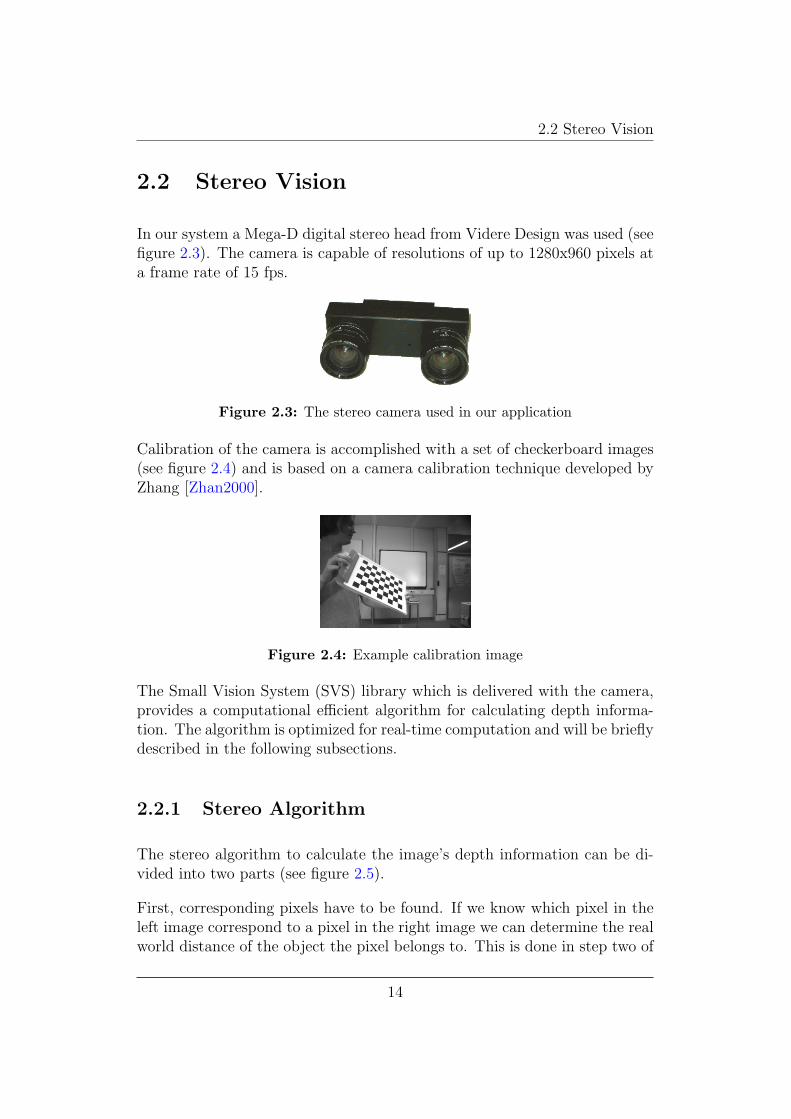
In our system a Mega-D digital stereo head from Videre Design was used (seefigure 2.3). The camera is capable of resolutions of up to 1280x960 pixels ata frame rate of 15 fps.
Figure 2.3: The stereo camera used in our application
Calibration of the camera is accomplished with a set of checkerboard images(see figure 2.4) and is based on a camera calibration technique developed byZhang [Zhan2000].
Figure 2.4: Example calibration image
The Small Vision System (SVS) library which is delivered with the camera,provides a computational efficient algorithm for calculating depth informa-tion. The algorithm is optimized for real-time computation and will be brieflydescribed in the following subsections.
2.2.1 Stereo Algorithm
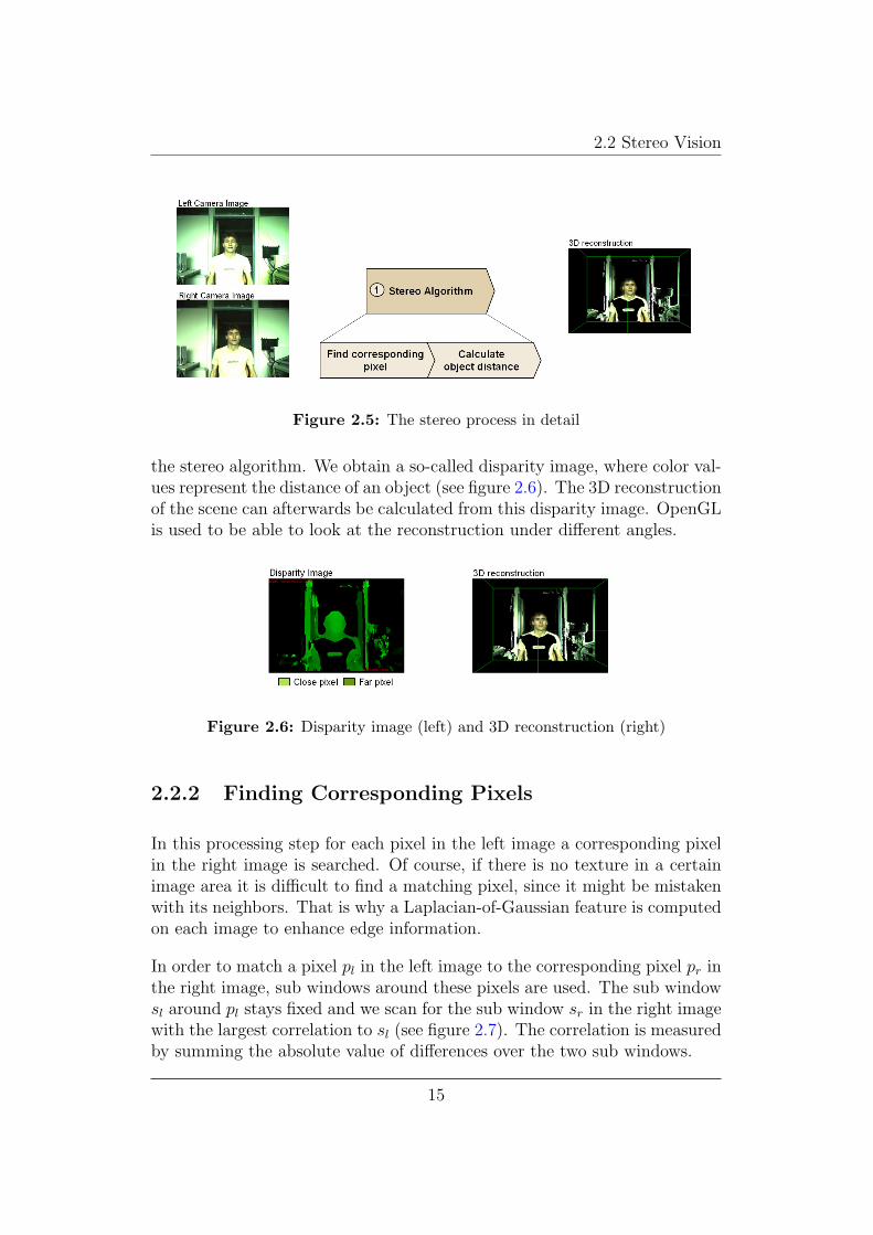
The stereo algorithm to calculate the image’s depth information can be di-vided into two parts (see figure 2.5).
First, corresponding pixels have to be found. If we know which pixel in theleft image correspond to a pixel in the right image we can determine the realworld distance of the object the pixel belongs to. This is done in step two of
14
2.2 Stereo Vision
Figure 2.5: The stereo process in detail
the stereo algorithm. We obtain a so-called disparity image, where color val-ues represent the distance of an object (see figure 2.6). The 3D reconstructionof the scene can afterwards be calculated from this disparity image. OpenGLis used to be able to look at the reconstruction under different angles.
Figure 2.6: Disparity image (left) and 3D reconstruction (right)
2.2.2 Finding Corresponding Pixels
In this processing step for each pixel in the left image a corresponding pixelin the right image is searched. Of course, if there is no texture in a certainimage area it is difficult to find a matching pixel, since it might be mistakenwith its neighbors. That is why a Laplacian-of-Gaussian feature is computedon each image to enhance edge information.
In order to match a pixel pl in the left image to the corresponding pixel pr inthe right image, sub windows around these pixels are used. The sub windowsl around pl stays fixed and we scan for the sub window sr in the right imagewith the largest correlation to sl (see figure 2.7). The correlation is measuredby summing the absolute value of differences over the two sub windows.
15

2.2 Stereo Vision
Figure 2.7: Finding corresponding pixels via the comparison of image windows
To double-check if the matched pixels pr and pl really belong together, thesame procedure is performed the other way round. The sub window sr aroundthe pixel pr in the right image stays fixed and the most correlated subunit inthe left image is searched. If this results in the known sub window sl around pl
the search has been consistent and will be accepted. This technique is calledleft-right check and is particularly effective in eliminating match errors innon-textured regions of the image, and at disparity boundaries.
Finally, post-filtering is performed. A confidence measure based on edgeenergy is used to eliminate matches whose confidence is below a certainthreshold. This threshold can be adjusted manually.
2.2.3 Calculating Object Distance
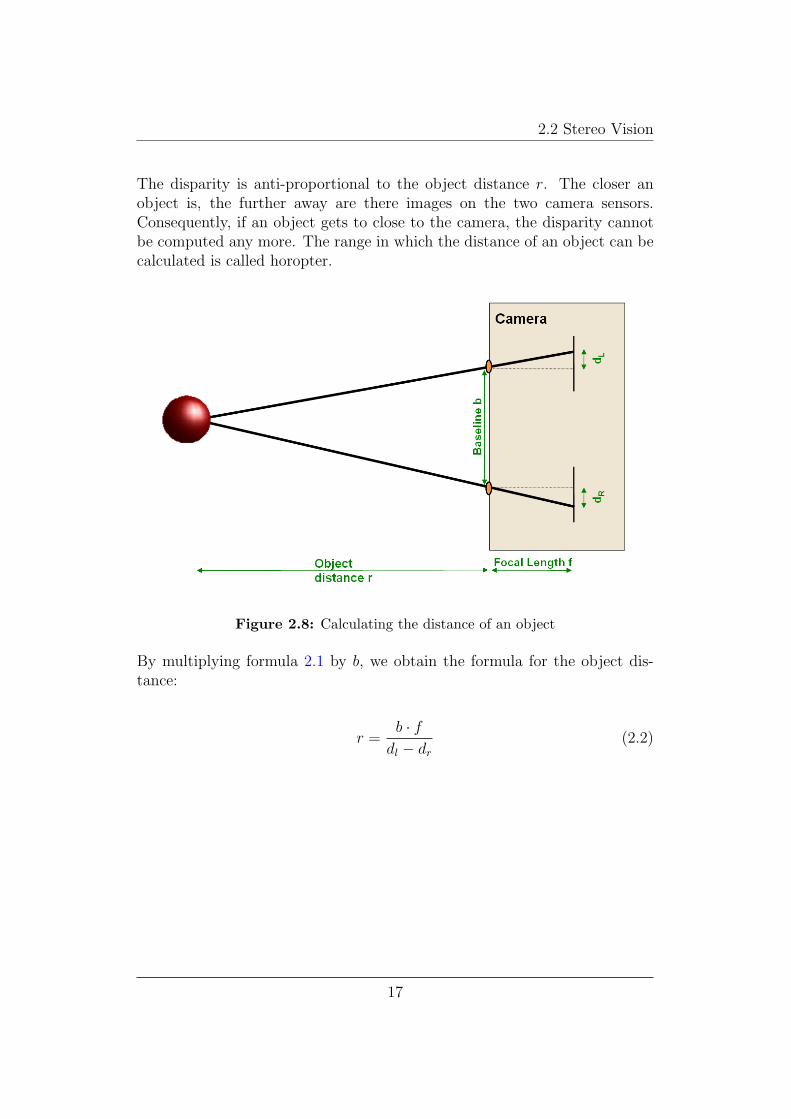
If we know which pixel in the left image correspond to which pixel in theright image, we can now calculate the distance a pair of pixels. This isaccomplished by a simple formula which follows from the intercept theorems.
As you can see in figure 2.8, we have the following interrelationship:
r
b=
f
dl − dr
(2.1)
where r is the object distance, b the length of the camera baseline, f thefocal length of the camera lens. dl and dr are the distances of the pixelsmatched pixels pl and pr from the sensor center. The difference dl − dr iscalled disparity (see [Jahn1997]).
16
2.2 Stereo Vision
The disparity is anti-proportional to the object distance r. The closer anobject is, the further away are there images on the two camera sensors.Consequently, if an object gets to close to the camera, the disparity cannotbe computed any more. The range in which the distance of an object can becalculated is called horopter.
Figure 2.8: Calculating the distance of an object
By multiplying formula 2.1 by b, we obtain the formula for the object dis-tance:
r =b · f
dl − dr
(2.2)
17
2.3 Face Detection and Extraction
2.3 Face Detection and Extraction
Robust face detection is crucial for head pose estimation. Without the correctposition of the head no useful head orientation can be computed. In thissection a head detection and extraction technique will be presented which isreliable and operates in real-time.
2.3.1 Pattern-Based Vs. Color-Based Face Detection
Two main approaches for face detection are distinguished.
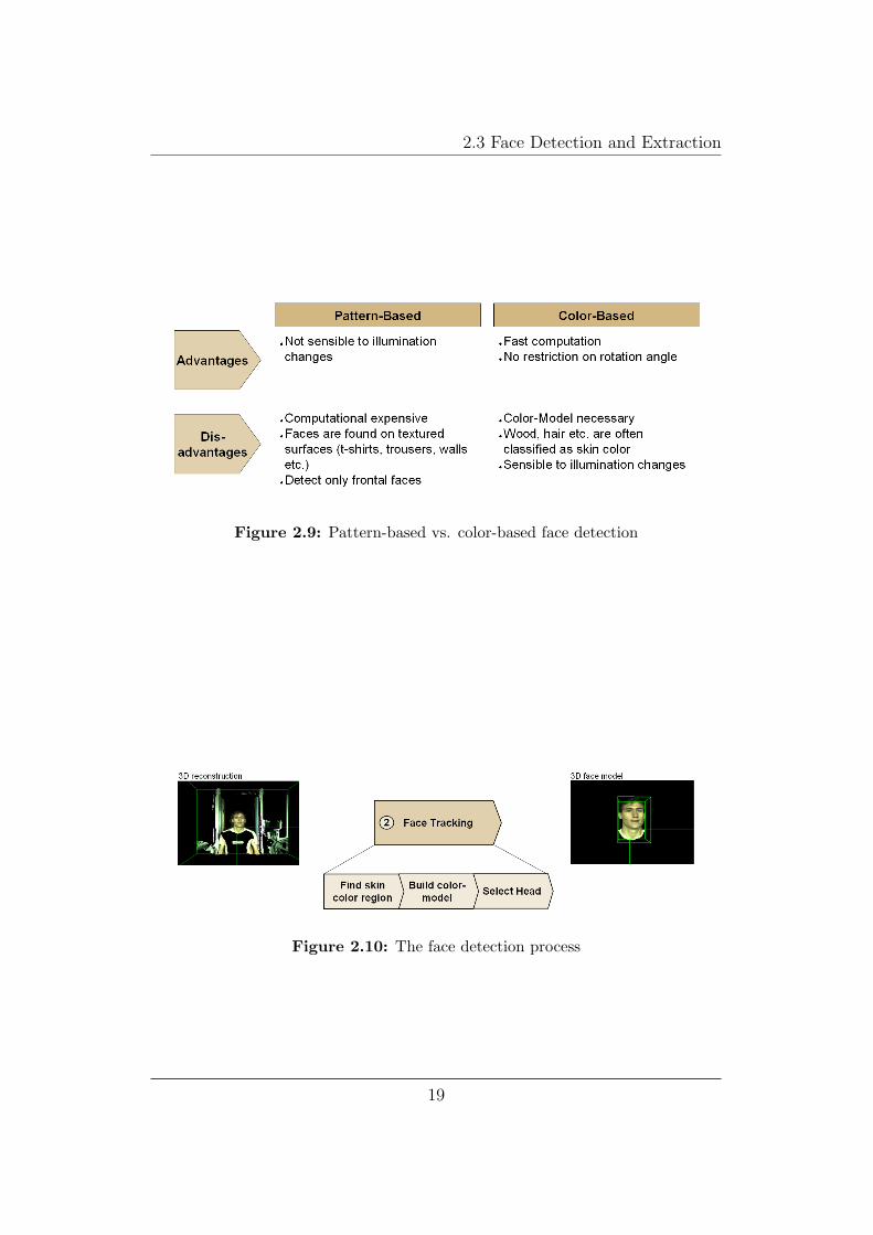
Pattern-based techniques scan for image areas that have the characteristicsof a human face. They do not depend on color information and are hardlysensible to illumination changes. Unfortunately, pattern-based techniquestend to be computational expensive, especially on high-resolution images.Moreover, faces may be found on random structured surfaces like trousers, t-shirts etc. A further disadvantage is that non-frontal faces are hard to detectwith pattern-based methods.
Color-based techniques on the contrary are rather fast, since they restrict thesearch area to skin-colored regions. However, to determine these regions acolor-model has to be built. Skin color changes under different lighting con-ditions and the color-model has therefore to be adapted to ensure robustness.An advantage of color-based methods is that they are easily able to detectnon-frontal faces. On the other hand, wood and hair are often confoundedwith skin-colored regions.
Figure 2.9 shows a quick comparison of the two face detection approaches.
In order to incorporate the advantage of both techniques, we implemented acombination of them in our system. A pattern-based face detector is used tofind an initial skin-colored region. On the basis of this region a color-modelis built. Subsequently, a color-based face detector extracts the face fromthe image. To improve detection performance the color-based face detectormakes use of the depth information obtained from the stereo algorithm.
Figure 2.10 shows an overview of the face detection process.
18
2.3 Face Detection and Extraction
Figure 2.9: Pattern-based vs. color-based face detection
Figure 2.10: The face detection process
19
2.3 Face Detection and Extraction
2.3.2 Finding A Skin Color Region
A skin-colored region can be used to create a color-model, which is adaptedto the current lighting conditions (see 2.3.3). There are various possibilitiesfor retrieving such a region from the image.
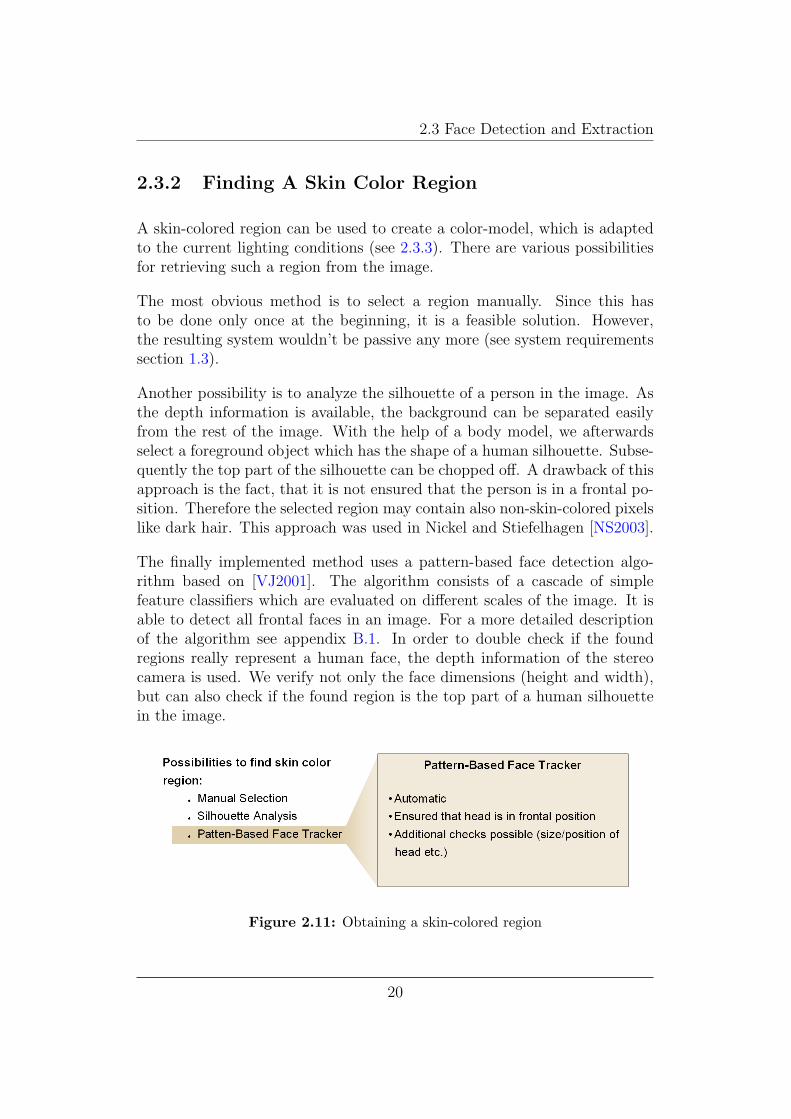
The most obvious method is to select a region manually. Since this hasto be done only once at the beginning, it is a feasible solution. However,the resulting system wouldn’t be passive any more (see system requirementssection 1.3).
Another possibility is to analyze the silhouette of a person in the image. Asthe depth information is available, the background can be separated easilyfrom the rest of the image. With the help of a body model, we afterwardsselect a foreground object which has the shape of a human silhouette. Subse-quently the top part of the silhouette can be chopped off. A drawback of thisapproach is the fact, that it is not ensured that the person is in a frontal po-sition. Therefore the selected region may contain also non-skin-colored pixelslike dark hair. This approach was used in Nickel and Stiefelhagen [NS2003].
The finally implemented method uses a pattern-based face detection algo-rithm based on [VJ2001]. The algorithm consists of a cascade of simplefeature classifiers which are evaluated on different scales of the image. It isable to detect all frontal faces in an image. For a more detailed descriptionof the algorithm see appendix B.1. In order to double check if the foundregions really represent a human face, the depth information of the stereocamera is used. We verify not only the face dimensions (height and width),but can also check if the found region is the top part of a human silhouettein the image.
Figure 2.11: Obtaining a skin-colored region
20
2.3 Face Detection and Extraction
2.3.3 Building The Color-Model
The Chromatic Color Space
Yang, Lu and Waibel [YLW1997] showed that skin color agglomerates ina small region in the chromatic color space (also referred to as rg-space).Therefore skin color classification can be done by defining a skin color distri-bution in rg-space. Two different representations for skin color distributionare distinguished. Parametric models like e.g. a mixture of Gaussians andnon-parametric models like i.e. histograms. In this work an adapted versionof the color-model from [NS2003] is used which is based on histograms.
The transformation from the RGB color space to the rg-space is done by thefollowing equations:
r =R
R + G + B, g =
G
R + G + B(2.3)
Colors in the rg-space are intensity normalized, which means that RGB-colorswith the same hue, but different intensity values are projected to the samerg-color.
A Histogram-Based Color-Model
Starting from the known skin color region (see subsection 2.3.2), histogramscan be build. We define the histograms H+ and H−:
H+(x) = Number of x in skin color region, x ∈ rg-space (2.4)
H−(x) = Number of x not in skin color region, x ∈ rg-space (2.5)
The histogram value H+ represents the frequency of a certain color value inthe skin color region. Thus, the relative frequency:
P+(x) =H+(x)
nwith n total number of pixels in the region (2.6)
21
2.3 Face Detection and Extraction
represents the empiric probability for x under the condition that x is skincolor. Hence, we have:
p(x|skin) = P+(x) (2.7)
However, we are actually interested in the probability p(skin|x), which meansthe probability for skin color under the condition, that we observe a pixelwith color x. Luckily, Bayes’ Rule helps us to compute this probability:
p(skin|x) =p(x|skin) · p(skin)
p(x)(2.8)
Like p(x|skin) the terms p(skin) and p(x) can be calculated empirically.P (skin) is just the ratio of the number of pixels in the known skin colorregion to the total number of pixels n. And p(x) is the ratio of the numberof pixels with color x to n.
Analogously, the probability p(notskin|x) can be computed out of the his-togram values H−(x). Consequently, a pixel l with color x is only consideredto be skin-colored, if the following holds:
p(skin|x)
p(not skin|x)> 1 (2.9)
Moreover, the higher this ratio, the more probable is pixel l skin-colored.
The above color-model is adapted to the current lighting conditions. If theillumination changes, the color-model has to be readapted accordingly. Thisis done, when the detection of a head in the image fails for several frames.
2.3.4 Face Extraction
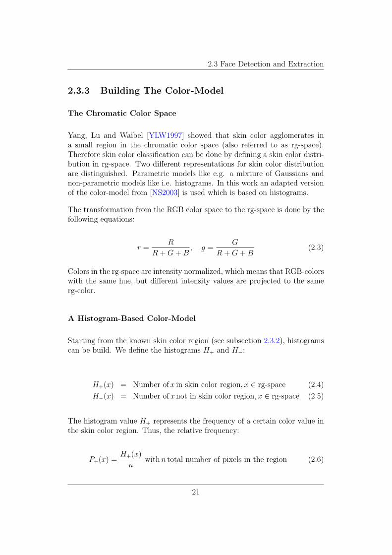
As mentioned in the last subsection the color-model can be used to classifypixels by skin color probability. Figure 2.12 shows the result of such a clas-sification. Darker points represent pixels with high skin color probability,brighter ones pixels with low skin color probability. White pixels representpixels where equation 2.9 does not hold. In the following, we will refer tothis representation as probability map.
22
2.3 Face Detection and Extraction
Figure 2.12: Pixels classified by skin color probabilities
Morphological Filtering
In order to obtain skin color regions from the above probability map, we haveto find clusters of skin-colored points. For this purpose we use morphologicalfiltering, which forms connected regions in the probability map.
Morphological filtering is based on two operations: dilatation and erosion.The dilatation operation sets the value of a pixel in the probability map tothe the maximum of its neighbors. The erosion operation, on the other hand,sets the value to the minimum of its neighbors.
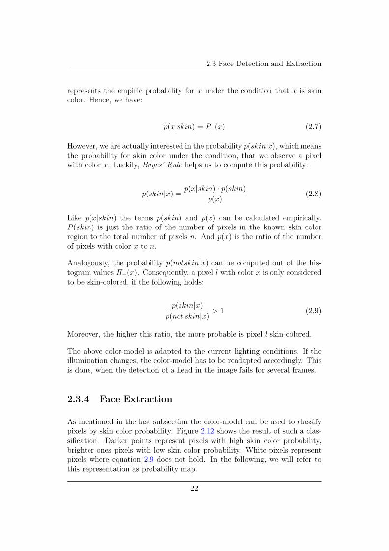
The neighborhood of a pixel can be defined arbitrarily. Common neighbor-hoods are 4-connectivity or 8-connectivity (see figure 2.13). The neighbor-hood is also referred to as structuring element.
Figure 2.13: Structuring elements for morphological filtering
In our system, we utilize the 8-connectivity structuring element.
On binary images dilatation augments the number of pixels with value 1,erosion on the other side removes them. dilatation and erosion are oftenapplied in combination. An erosion operation followed by a dilatation iscalled morphological opening, a dilatation operation followed by an erosionmorphological closing. Figure 2.14 shows how morphological closing with a2x1 structuring element removes a hole in an object.
23

2.3 Face Detection and Extraction
Dilatation Erosion
Figure 2.14: Morphological closing with a 2x1 structure element removes hole inobject
This is exactly what we want to do in our application. The isolated skincolor pixels should be grouped to skin color region or blobs. By applyinga morphological closing operation we can obtain these connected skin colorregions (see figure 2.15).
Figure 2.15: Skin color blobs resulting from morphological filtering
Verifying Position and Dimensions
What still needs to be done, is the selection of the skin color blob, whichcorresponds to a head in the original image. This is accomplished by verifyingthe position and dimensions of the blobs.
In section 2.2 it has been showed how the distance of an object can bedetermined with stereo vision. Knowing the distance of an object enables usnot only to calculate the 3D position of the object, but also to compute thereal-world size of the object. As for the distance calculation this can be doneby applying intercept theorems:
ps
f=
rs
b(2.10)
24
2.3 Face Detection and Extraction
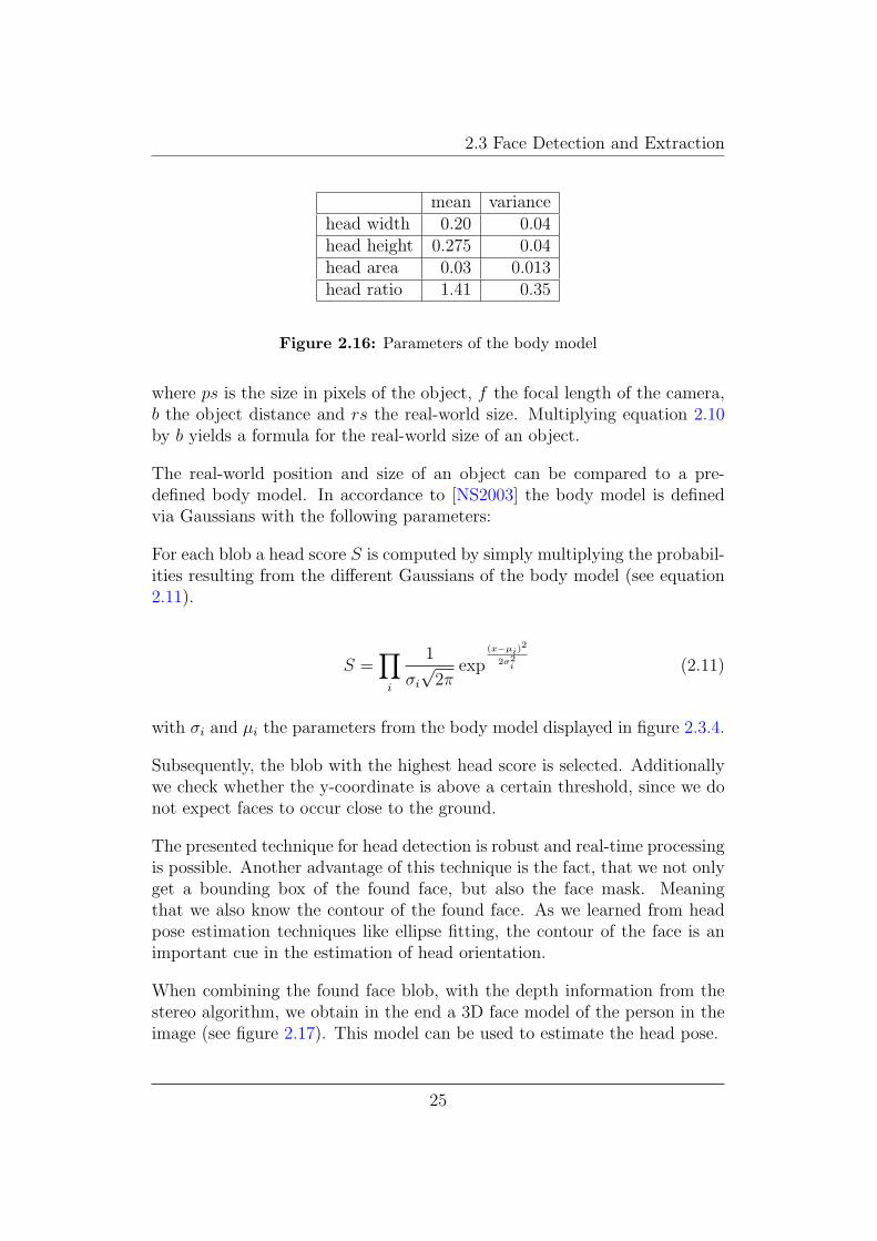
mean variancehead width 0.20 0.04head height 0.275 0.04head area 0.03 0.013head ratio 1.41 0.35
Figure 2.16: Parameters of the body model
where ps is the size in pixels of the object, f the focal length of the camera,b the object distance and rs the real-world size. Multiplying equation 2.10by b yields a formula for the real-world size of an object.
The real-world position and size of an object can be compared to a pre-defined body model. In accordance to [NS2003] the body model is definedvia Gaussians with the following parameters:
For each blob a head score S is computed by simply multiplying the probabil-ities resulting from the different Gaussians of the body model (see equation2.11).
S =∏
i
1
σi
√2π
exp(x−µi)
2
2σ2i (2.11)
with σi and µi the parameters from the body model displayed in figure 2.3.4.
Subsequently, the blob with the highest head score is selected. Additionallywe check whether the y-coordinate is above a certain threshold, since we donot expect faces to occur close to the ground.
The presented technique for head detection is robust and real-time processingis possible. Another advantage of this technique is the fact, that we not onlyget a bounding box of the found face, but also the face mask. Meaningthat we also know the contour of the found face. As we learned from headpose estimation techniques like ellipse fitting, the contour of the face is animportant cue in the estimation of head orientation.
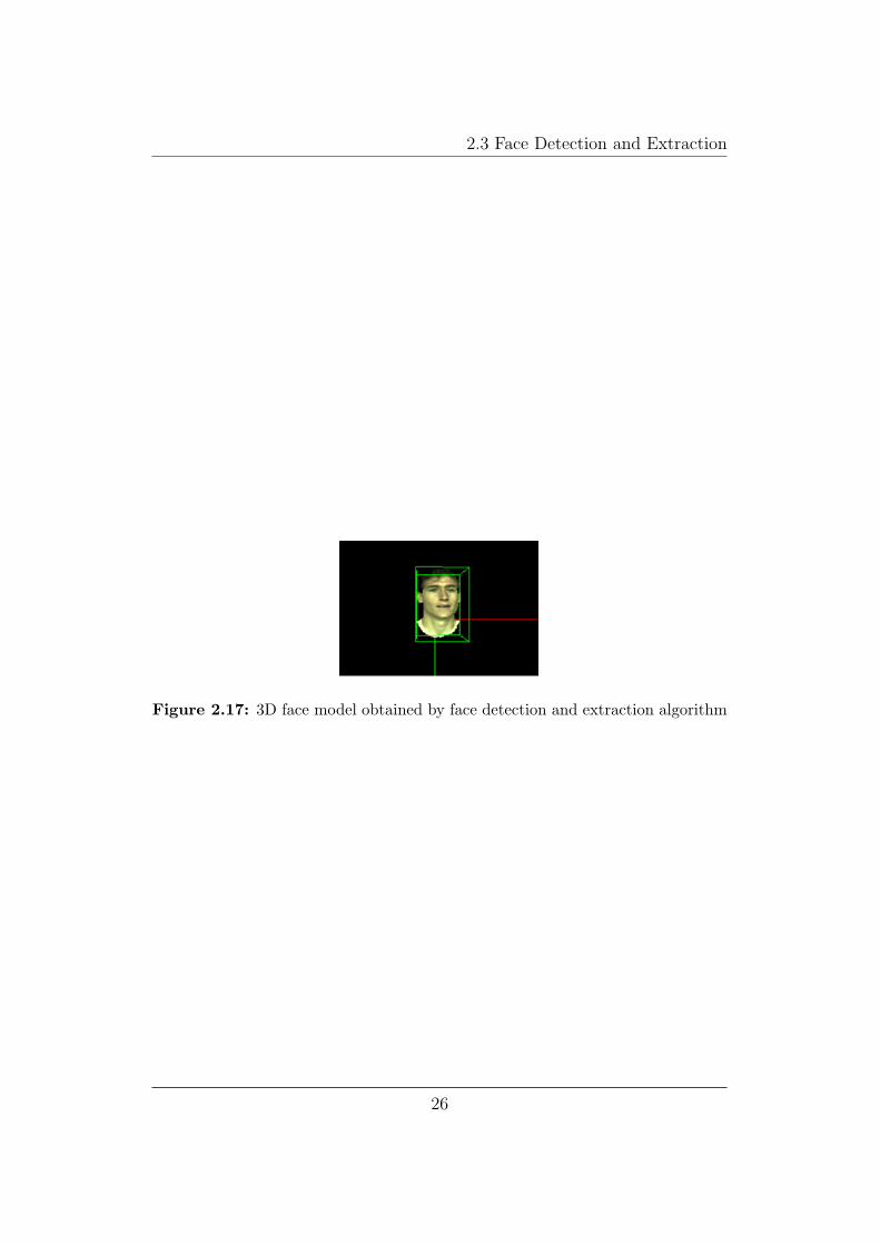
When combining the found face blob, with the depth information from thestereo algorithm, we obtain in the end a 3D face model of the person in theimage (see figure 2.17). This model can be used to estimate the head pose.
25
2.3 Face Detection and Extraction
Figure 2.17: 3D face model obtained by face detection and extraction algorithm
26
2.4 Preprocessing
2.4 Preprocessing
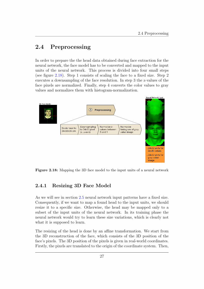
In order to prepare the the head data obtained during face extraction for theneural network, the face model has to be converted and mapped to the inputunits of the neural network. This process is divided into four small steps(see figure 2.18). Step 1 consists of scaling the face to a fixed size. Step 2executes a downsampling of the face resolution. In step 3 the z-values of theface pixels are normalized. Finally, step 4 converts the color values to grayvalues and normalizes them with histogram-normalization.
Figure 2.18: Mapping the 3D face model to the input units of a neural network
2.4.1 Resizing 3D Face Model
As we will see in section 2.5 neural network input patterns have a fixed size.Consequently, if we want to map a found head to the input units, we shouldresize it to a specific size. Otherwise, the head may be mapped only to asubset of the input units of the neural network. In its training phase theneural network would try to learn these size variations, which is clearly notwhat it is supposed to learn.
The resizing of the head is done by an affine transformation. We start fromthe 3D reconstruction of the face, which consists of the 3D position of theface’s pixels. The 3D position of the pixels is given in real-world coordinates.Firstly, the pixels are translated to the origin of the coordinate system. Then,
27
2.4 Preprocessing
we scale the face by multiplying the pixel coordinates with a diagonal trans-formation matrix. For the new 3D coordinate of a pixel, we obtain thefollowing formula:
xnew
ynew
znew
=
xyz
−
txtytz
·
sx 0 00 sy 00 0 sz
(2.12)
where tx, ty, tz denote the translation vector to the origin and sx, sy, sz denotethe scaling factors in x-, y- and z-direction.
Since we use 24x32 input units for the neural network the scaling factors arecalculated such that the bounding box of the head is resized to 24x32cm.Remember that the pixel are given in real-world coordinates. The boundingbox is defined as the smallest box to enclose all pixels of the face model.
2.4.2 Downsampling
To obtain exactly 24x32 gray respectively depth values from the face model,we divide the bounding box of the head into a three dimensional grid withgrid distance 1 cm. For every 1 cm cube within this grid, we calculate arepresentative pixel out of the information of all pixels in the cube.
This representative pixel may be computed in various ways, e.g.:
• taking the average of colors and coordinates
• taking the median of color and coordinates
• taking the values of a random pixel
Since pixels in a cube tend to be very similar, in our system we simplyselected a random pixel.
As a result of this step we obtain a face model consisting of solely 24x32pixels in 3D space.
28

2.4 Preprocessing
2.4.3 Depth normalization
Before the depth values are normalized, color and depth information areseparated. This needs to be done, because the activation of the input unitsof the neural network may only be described by a single value. Hence, inthe following we map the depth information of the face pixels to 24x32 inputunits of the neural network and we map the color model to another 24x32input units of the neural network. In total we therefore obtain a neuralnetwork input layer with 2x24x32 units.
As we will see in section 2.5 each neural network unit has an associatedactivation function. The activation function we use in our system is a logisticfunction yielding values between 0 and 1. Therefore our initial activations(the activations of the input units) should also be in the range of 0 to 1. Anaffine transformation in z-direction scales down our face model accordingly.
2.4.4 Gray Value Normalization
The intensities of gray values differ under changing lighting conditions. Asfor the size variations, we do not want the neural network to learn differentintensity levels. Consequently a way of compensating these differences hasto be found.
In our system a technique has been implemented, which tries to equalizethe gray value histogram H of a input pattern. It starts off by building theaccumulated histogram M . M is defined in the following manner:
M(x) =
∫z≤x
H(z)dz for the continuous case (2.13)
M(x) =∑z≤x
H(z) for the discrete case (2.14)
The new gray value xnew of a pixel with the current gray value x is subse-quently computed from M with the below formula:
xnew = M(x) (2.15)
29

2.4 Preprocessing
As a result of this mapping, we obtain a histogram of the new gray valuesxnew which is distributed equally. This is due to the fact that the valuesxnew change faster in areas where M grows rapidly. Since rapid growth ofM at x corresponds to a high number of pixels with gray value x, this kindof mapping spreads the new gray values in this region and therefore lessensextrema of the histogram.
A further enhancement of this technique is also utilized in [HB1995]. There,this technique is used not only to equalize histograms, but also to matchan image’s histogram to an arbitrary distribution. They call this techniquehistogram matching.
30
2.5 Estimating Head Pose With Neural Networks
2.5 Estimating Head Pose With Neural Net-
works
In the previous sections we have seen how the data has been prepared forthe final estimation of the head pose. Now, we want to have a look at howthe estimation is actually performed with a neural network.
For a quick theoretical introduction to neural networks and neural networklearning algorithms please refer to appendix A.
2.5.1 Neural Network Topology
When dealing with neural networks, we first have to decide which topologywe want to use. Determining an optimal topology is a difficult problem andhas been studied extensively (see for example [SM2002] and [Matt2002]).
Usually one starts out by first determining the number of input units. Inmost cases their number is rather obvious, since there have to be as muchinput units as the number of elements in the data vector we want to classify.However, the more input units a neural network has the more training data isnecessary to train it appropriately. Consequently, techniques for reducing thedimensionality are often applied to the initial data vector in preprocessing.
In our system, the dimensionality reduction has been performed by simplysampling down the 3D face model to the relatively small size of 24x32 points.In other applications techniques like principal component analysis (PCA) areused for this purpose.
Thus, in our system the input layer of the network consists of 1536 units,which corresponds to 24x32 units for the gray value information and 24x32pixels for the depth information. As we will see in chapter 3, additionally wetrained a network which uses only the gray value information. This networkhas 768 input units.
The next problem that is usually considered, is the number output units.Again, this number is in most cases straight forward, since there have to beas much output units as classes which we try to distinguish.
For our application, this means that we would have to divide our continuous
31

2.5 Estimating Head Pose With Neural Networks
output space, the rotation angles between −90◦ and +90◦, into angle ranges.Consequently, an output unit corresponding to a certain angle range wouldhave a high activation, if the real rotation angle is contained in this anglerange. All other output units might also have an activation, however, theiractivation should be smaller.
In experiments, however, a function approximation approach proved supe-rior results. Unlike neural network classification, in this case only a singleoutput unit is used. The activation of this output unit isn’t interpreted asa probability measure for classification, but directly as the desired rotationangle. Hence, during training the neural network was provided by an inputpattern containing gray value and depth information and the target angle forthe output unit normalized between 0 and 1.
Another performance improvement has been obtained by training separatenetworks for each degree of freedom. Thus, in the final network for estimatingone of the rotation angles, the network contained 1536 input units and a singleoutput unit.
What still needs to be decided is the number of hidden layers and hidden unitsthe neural network should contain. As mentioned in appendix A feed-forwardnetworks with two-layers of weights and sigmoidal activation functions canapproximate any decision boundary to arbitrary accuracy (see [Krei1991]),if the number of hidden units is sufficiently high.
Consequently, a neural network containing the 1536 input units, one outputunit and a hidden unit layer with a so far undefined number of units shouldbe able to estimate the angles accurately. A pre-condition, however, is thatthere is a sufficiently large training data.
Our experiments showed that an amount of 60 to 80 units in the hiddenlayer of the neural network was suited best for estimating the head orien-tation accurately. In the experiments each unit layer was fully-connectedwith the successive layer. This means that each unit of the input layer wasconnected to each unit of the hidden layer and each unit of the hidden layerwas connected with the output unit. Surprisingly, even with a much higherand smaller number for the hidden units, the network still achieved rathergood results.
To sum it up, our neural network contained three layers of units:
• 1536 units in the input layer
32

2.5 Estimating Head Pose With Neural Networks
• 60-80 units in the hidden layer
• 1 unit in the output layer
These layers were fully connected and contained only forward connections,meaning that there are no cycles of weights in the network.
Figure 2.19 shows a picture of the network.
Figure 2.19: The topology of the neural network
2.5.2 Advantages Of This Approach
There are several advantages of this approach. Firstly, there exist a powerfuland computational efficient algorithm for neural network learning: error-backpropagation. Next to the standard back-propagation algorithm whichwas used in this work, there are even more sophisticated learning algorithmlike, for example QuickProp or RProp. These algorithms improve the con-vergence speed during neural network training.
Unlike other head pose estimation techniques (see section 1.4), the neuralnetworks do not estimate the relative head rotation from one frame to an-other, but directly compute the orientation from a single image frame. Thatis why the estimation errors aren’t accumulated over an image sequence. This
33

2.5 Estimating Head Pose With Neural Networks
effect is called drift and is a significant drawback of approaches using, for ex-ample, optical flow. Furthermore when only relative rotations are estimated,the initial head orientation of a person has to be known. Thus, a manualinitialization is required. For neural networks no manual initialization isnecessary.
Another advantage is, that the above network topology does not divide theestimation in angle ranges or classes. Consequently, the real head orientationscan be approximated very precisely.
Once neural networks are trained, they are extremely fast in computation.The activation levels of the input patterns have simply to be propagatedthrough the three layers of the network. Hence, they are well suited for areal-time head pose estimation technique.
34

Chapter 3
Experimental Results
For evaluating the system described in the previous chapter, video data setsin different environments have been recorded. On the acquired data, a num-ber of experiments have been run and the system’s performance has beenanalysed. In the following we’ll describe the results of these experiments andthe conditions under which the video data has been recorded.
3.1 Data Collection “Portrait View”
The “Portrait View” data collection has been recorded in a relatively re-stricted environment. People were sitting in about 2 meter distance in frontof the stereo camera. Therefore the position of the head in the image did notchange considerably.
However, the people’s movement wasn’t restricted in any way. They werefree to move their heads in pan, tilt and roll direction (see figure 3.1).
Figure 3.1: Pan, tilt and roll angles (image based on [Fitz2001])
35
3.1 Data Collection “Portrait View”
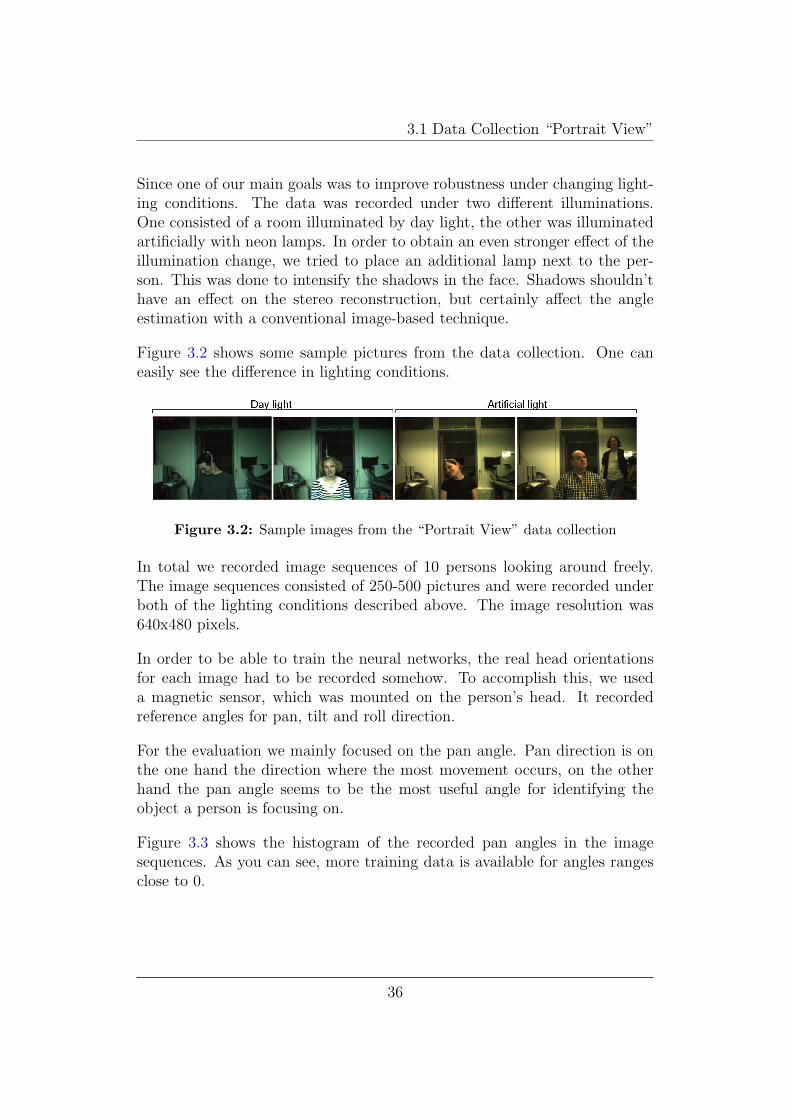
Since one of our main goals was to improve robustness under changing light-ing conditions. The data was recorded under two different illuminations.One consisted of a room illuminated by day light, the other was illuminatedartificially with neon lamps. In order to obtain an even stronger effect of theillumination change, we tried to place an additional lamp next to the per-son. This was done to intensify the shadows in the face. Shadows shouldn’thave an effect on the stereo reconstruction, but certainly affect the angleestimation with a conventional image-based technique.
Figure 3.2 shows some sample pictures from the data collection. One caneasily see the difference in lighting conditions.
Figure 3.2: Sample images from the “Portrait View” data collection
In total we recorded image sequences of 10 persons looking around freely.The image sequences consisted of 250-500 pictures and were recorded underboth of the lighting conditions described above. The image resolution was640x480 pixels.
In order to be able to train the neural networks, the real head orientationsfor each image had to be recorded somehow. To accomplish this, we useda magnetic sensor, which was mounted on the person’s head. It recordedreference angles for pan, tilt and roll direction.
For the evaluation we mainly focused on the pan angle. Pan direction is onthe one hand the direction where the most movement occurs, on the otherhand the pan angle seems to be the most useful angle for identifying theobject a person is focusing on.
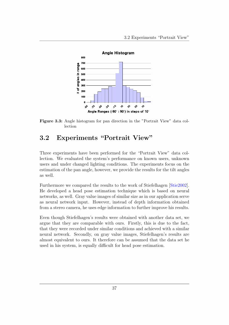
Figure 3.3 shows the histogram of the recorded pan angles in the imagesequences. As you can see, more training data is available for angles rangesclose to 0.
36
3.2 Experiments “Portrait View”
Figure 3.3: Angle histogram for pan direction in the ”Portrait View” data col-lection
3.2 Experiments “Portrait View”
Three experiments have been performed for the “Portrait View” data col-lection. We evaluated the system’s performance on known users, unknownusers and under changed lighting conditions. The experiments focus on theestimation of the pan angle, however, we provide the results for the tilt anglesas well.
Furthermore we compared the results to the work of Stiefelhagen [Stie2002].He developed a head pose estimation technique which is based on neuralnetworks, as well. Gray value images of similar size as in our application serveas neural network input. However, instead of depth information obtainedfrom a stereo camera, he uses edge information to further improve his results.
Even though Stiefelhagen’s results were obtained with another data set, weargue that they are comparable with ours. Firstly, this is due to the fact,that they were recorded under similar conditions and achieved with a similarneural network. Secondly, on gray value images, Stiefelhagen’s results arealmost equivalent to ours. It therefore can be assumed that the data set heused in his system, is equally difficult for head pose estimation.
37
3.2 Experiments “Portrait View”
3.2.1 Test 1 - Known Users
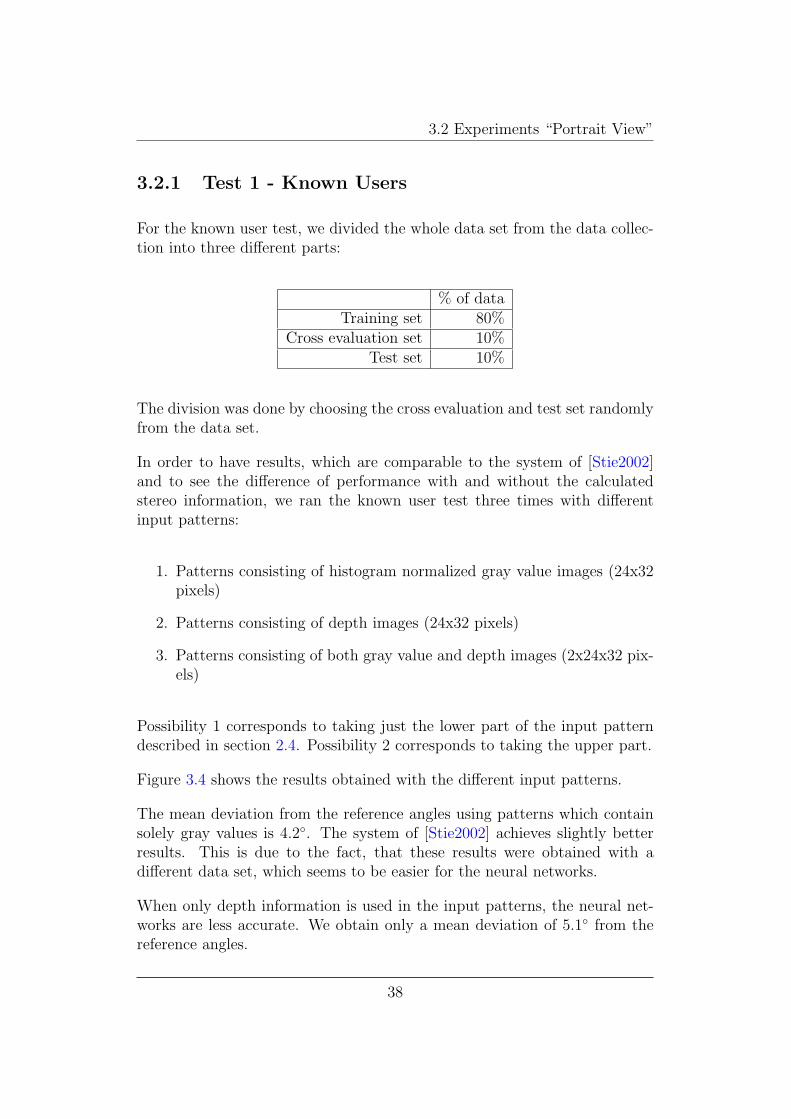
For the known user test, we divided the whole data set from the data collec-tion into three different parts:
% of dataTraining set 80%
Cross evaluation set 10%Test set 10%
The division was done by choosing the cross evaluation and test set randomlyfrom the data set.
In order to have results, which are comparable to the system of [Stie2002]and to see the difference of performance with and without the calculatedstereo information, we ran the known user test three times with differentinput patterns:
1. Patterns consisting of histogram normalized gray value images (24x32pixels)
2. Patterns consisting of depth images (24x32 pixels)
3. Patterns consisting of both gray value and depth images (2x24x32 pix-els)
Possibility 1 corresponds to taking just the lower part of the input patterndescribed in section 2.4. Possibility 2 corresponds to taking the upper part.
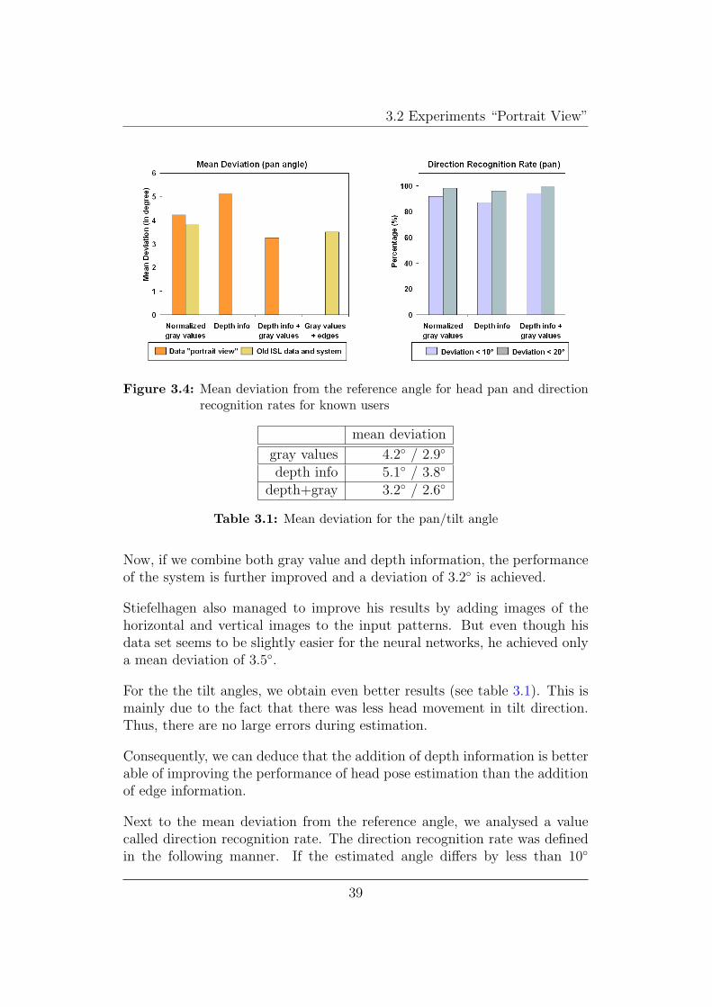
Figure 3.4 shows the results obtained with the different input patterns.
The mean deviation from the reference angles using patterns which containsolely gray values is 4.2◦. The system of [Stie2002] achieves slightly betterresults. This is due to the fact, that these results were obtained with adifferent data set, which seems to be easier for the neural networks.
When only depth information is used in the input patterns, the neural net-works are less accurate. We obtain only a mean deviation of 5.1◦ from thereference angles.
38
3.2 Experiments “Portrait View”
Figure 3.4: Mean deviation from the reference angle for head pan and directionrecognition rates for known users
mean deviation
gray values 4.2◦ / 2.9◦
depth info 5.1◦ / 3.8◦
depth+gray 3.2◦ / 2.6◦
Table 3.1: Mean deviation for the pan/tilt angle
Now, if we combine both gray value and depth information, the performanceof the system is further improved and a deviation of 3.2◦ is achieved.
Stiefelhagen also managed to improve his results by adding images of thehorizontal and vertical images to the input patterns. But even though hisdata set seems to be slightly easier for the neural networks, he achieved onlya mean deviation of 3.5◦.
For the the tilt angles, we obtain even better results (see table 3.1). This ismainly due to the fact that there was less head movement in tilt direction.Thus, there are no large errors during estimation.
Consequently, we can deduce that the addition of depth information is betterable of improving the performance of head pose estimation than the additionof edge information.
Next to the mean deviation from the reference angle, we analysed a valuecalled direction recognition rate. The direction recognition rate was definedin the following manner. If the estimated angle differs by less than 10◦
39
3.2 Experiments “Portrait View”
respectively 20◦ (see figure 3.4) from the reference angle, we consider thedirection to be recognized by the neural network.
Under these circumstances we obtain recognition rates of 91.8% and 98.1%(depending on the allowed deviation) with patterns consisting of gray valueimages. The depth information alone leads to recognition rates of 87% and95.9%. Neural networks that use patterns with a combination of gray valueand depth information recognize 94.3% and 99.7%.
As you can see the estimation of the pan angle for known users is ratheraccurate. However, for practical applications, we do not want the system todepend on the user. This would imply to retrain the network for every newuser. Since neural network training is computational expensive we want toavoid retraining.
In the next subsection we are evaluating the system’s performance on newusers.
3.2.2 Test 2 - Unknown Users
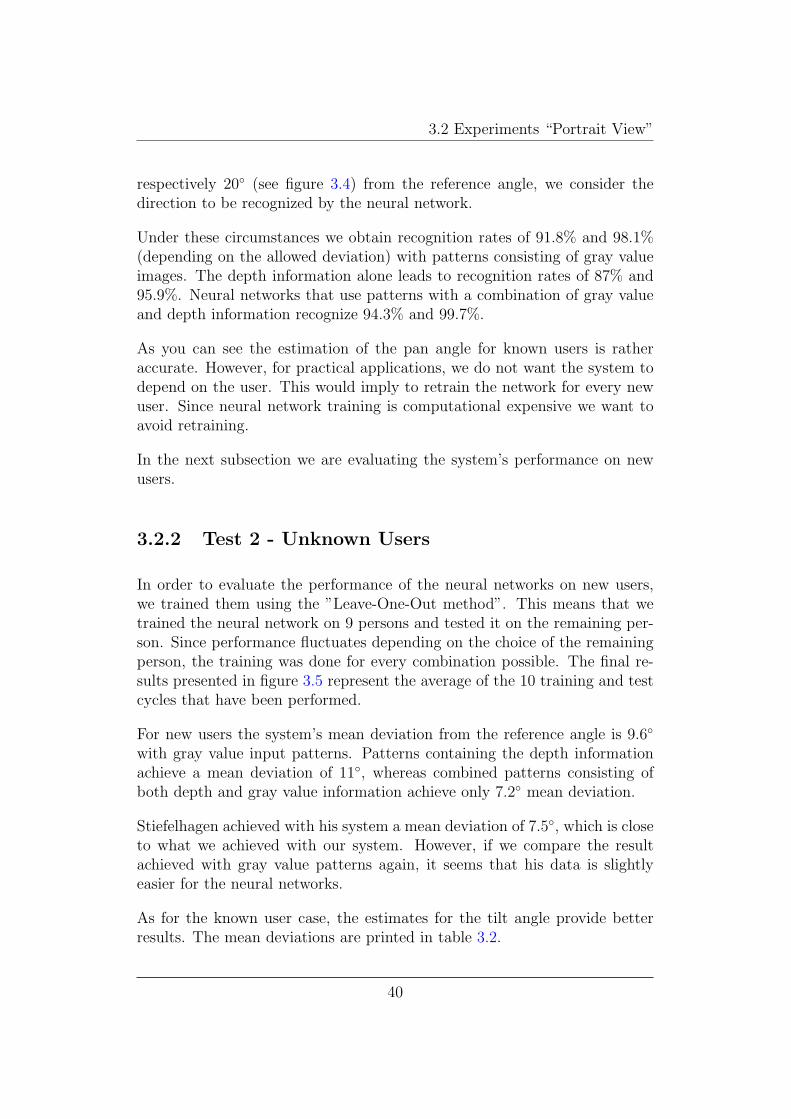
In order to evaluate the performance of the neural networks on new users,we trained them using the ”Leave-One-Out method”. This means that wetrained the neural network on 9 persons and tested it on the remaining per-son. Since performance fluctuates depending on the choice of the remainingperson, the training was done for every combination possible. The final re-sults presented in figure 3.5 represent the average of the 10 training and testcycles that have been performed.
For new users the system’s mean deviation from the reference angle is 9.6◦
with gray value input patterns. Patterns containing the depth informationachieve a mean deviation of 11◦, whereas combined patterns consisting ofboth depth and gray value information achieve only 7.2◦ mean deviation.
Stiefelhagen achieved with his system a mean deviation of 7.5◦, which is closeto what we achieved with our system. However, if we compare the resultachieved with gray value patterns again, it seems that his data is slightlyeasier for the neural networks.
As for the known user case, the estimates for the tilt angle provide betterresults. The mean deviations are printed in table 3.2.
40
3.2 Experiments “Portrait View”
Figure 3.5: Mean deviation from the reference angle for head pan and directionrecognition rates for unknown users
mean deviation
gray values 9.6◦ / 8.8◦
depth info 11.0◦ / 7.6◦
depth+gray 7.5◦ / 6.7◦
Table 3.2: Mean deviation for the pan/tilt angle for unknown users
These values are considerably worse than the results for known users. Thisis due to a number of circumstances. On the one hand the heads of persondiffer in appearance and aspect ratio. For example, some people’s headsare rather longish, whereas others have heads which are quite broad. Onthe other hand, the algorithm who extracts the heads from the image (seesection 2.3) might consider a person’s hair to belong or not to belong to thehead. Especially for people with long hair this is an issue.
As mentioned above, the presented values are average values. The rangeof the mean deviation was rather high. We observed values form 5◦ meandeviation up to 10.5◦ mean deviation depending on the person (with depth-gray input patterns).
As a matter of course the accuracy of the direction recognition rate decreasedalso when compared to the known user case. With gray value patterns recog-nition rates of 62.3% and 88.9% have been achieved. Depth information aloneled to a recognition rate of 51.8% and 84.3%. Depth and gray value infor-mation together resulted in an direction recognition accuracy of 75.2% and
41
3.2 Experiments “Portrait View”
95.1%.
It can be concluded that the use of depth information improves head poseestimation for unknown users, as well. Depth information alone, however, isnot sufficient for an accurate estimation.
3.2.3 Test 3 - Changed Lighting Conditions
Changing lighting conditions are one of the main problems of image-basedtechniques and particularly neural networks. Neural networks approximatefunctions, which map the neural network input to the output. Now, if theinput changes due to a different illumination, the learned function isn’t thesame any more.
As Stiefelhagen [Stie2002] has shown, histogram normalization helps com-pensating changing lighting conditions to a certain amount. However, theresults are still rather bad.
As we argued in the introduction of this work, depth information shouldbe greatly invariant towards illumination changes. Therefore, we traineda neural network under some lighting conditions and afterwards tested thealready trained network under the new illumination conditions.
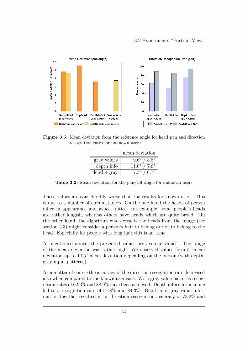
Figure 3.6 shows the results obtained in this case.
Figure 3.6: Mean deviation from the reference angle and direction recognitionrates for unknown users
42

3.2 Experiments “Portrait View”
The mean deviation from the reference angle with gray value patterns in-creases to 13.9◦. The combination of gray value and depth information leadsto a mean deviation of 10.6◦, whereas under these circumstances depth in-formations is with 9.6◦ mean deviation the most stable.
This is exactly what we expected. Depth information is indeed rather in-variant to illumination change and improves head pose estimation under thenew conditions considerably. In fact, when we compare this result to ”Test2” with unknown users from above, it can be seen, that the mean deviationis the same.
Stiefelhagen achieved with his system a mean deviation of 13.8◦. Edge infor-mation seems to be less suited for changing lighting conditions. This seemsto be reasonable, since edge information is strongly influenced by the illumi-nation conditions. Shadows, for example, produce edges in the face image,that are not really existent in the three dimensional scene.
For the direction recognition rates, the following results have been obtained.40.7% and 75.1% accuracy for gray value input patterns. Depth and grayvalue information yielded an accuracy of 56.9% and 86.2%. As for the meandeviation the best results, however, have been obtained with depth informa-tion alone. Here the direction recognition rates were 60% and 87.6%.
We conclude that depth information is suited best for head pose estimationunder changing lighting conditions. To have a versatile method working wellunder all conditions, we propose nevertheless to combine depth and grayvalue information for head pose estimation. With this configuration theconventional intensity image-based approach is still 31% worse.
3.2.4 Error Analysis
Error analysis cannot only help to understand where and why the errorsoccur, but also be useful to improve the performance of the estimation.
So, in order to better understand the head pose estimates, we analysed thepan estimation errors for different pan and tilt angle ranges. We expectedthe error of the estimation to be worse for large angles. On the one handbecause less training data was available, on the other hand because less of theface is visible and therefore it might be more difficult for the neural networkto find appropriate features.
43
3.2 Experiments “Portrait View”
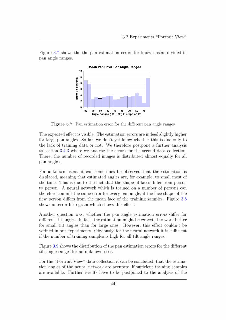
Figure 3.7 shows the the pan estimation errors for known users divided inpan angle ranges.
Figure 3.7: Pan estimation error for the different pan angle ranges
The expected effect is visible. The estimation errors are indeed slightly higherfor large pan angles. So far, we don’t yet know whether this is due only tothe lack of training data or not. We therefore postpone a further analysisto section 3.4.3 where we analyse the errors for the second data collection.There, the number of recorded images is distributed almost equally for allpan angles.
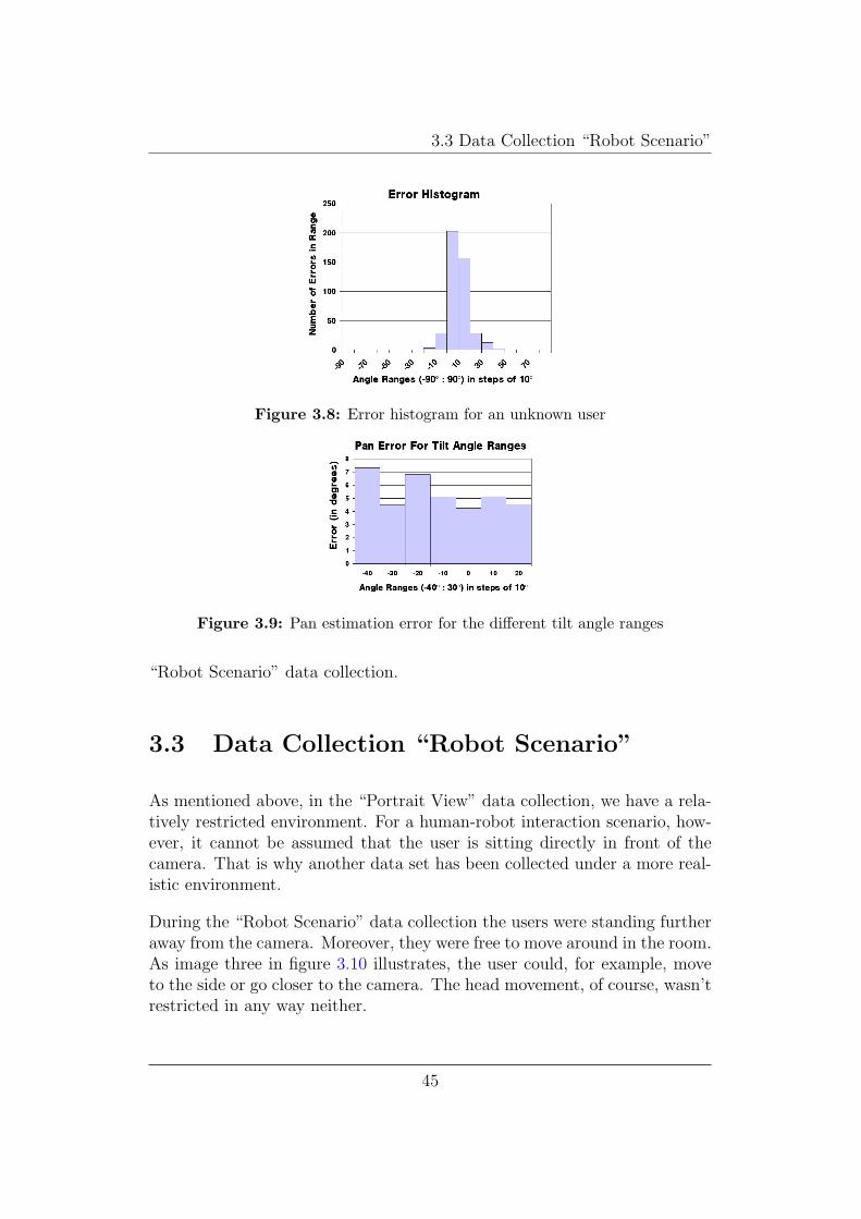
For unknown users, it can sometimes be observed that the estimation isdisplaced, meaning that estimated angles are, for example, to small most ofthe time. This is due to the fact that the shape of faces differ from personto person. A neural network which is trained on a number of persons cantherefore commit the same error for every pan angle, if the face shape of thenew person differs from the mean face of the training samples. Figure 3.8shows an error histogram which shows this effect.
Another question was, whether the pan angle estimation errors differ fordifferent tilt angles. In fact, the estimation might be expected to work betterfor small tilt angles than for large ones. However, this effect couldn’t beverified in our experiments. Obviously, for the neural network it is sufficientif the number of training samples is high for all tilt angle ranges.
Figure 3.9 shows the distribution of the pan estimation errors for the differenttilt angle ranges for an unknown user.
For the “Portrait View” data collection it can be concluded, that the estima-tion angles of the neural network are accurate, if sufficient training samplesare available. Further results have to be postponed to the analysis of the
44
3.3 Data Collection “Robot Scenario”
Figure 3.8: Error histogram for an unknown user
Figure 3.9: Pan estimation error for the different tilt angle ranges
“Robot Scenario” data collection.
3.3 Data Collection “Robot Scenario”
As mentioned above, in the “Portrait View” data collection, we have a rela-tively restricted environment. For a human-robot interaction scenario, how-ever, it cannot be assumed that the user is sitting directly in front of thecamera. That is why another data set has been collected under a more real-istic environment.
During the “Robot Scenario” data collection the users were standing furtheraway from the camera. Moreover, they were free to move around in the room.As image three in figure 3.10 illustrates, the user could, for example, moveto the side or go closer to the camera. The head movement, of course, wasn’trestricted in any way neither.
45

3.4 Experiments “Robot Scenario”
Since we later want to incorporate the recognition of hand gestures in thesystem. The users were additionally asked to execute pointing gestures onpre-defined targets in the room.
Figure 3.10: Sample images from the ”Robot Scenario” data collection
A total of six users have been recorded under these conditions. The datasequences consist of about 1000 images per person. Even though the headsin the images were smaller than for the ”Portrait View” data collection, theimage resolution wasn’t changed and remained at 640x480 pixels. Conse-quently the afterwards extracted head models consisted of fewer pixels. Butsince the data is downscaled for the neural network anyways, this shouldn’thave an effect on the system’s performance (as long as the heads are stillsufficiently large).
As for the “Portrait View” data collection the reference angles were capturedwith a magnetic sensor, which was mounted on the user’s head. Again wecaptured pan, tilt and roll angle for every frame in the data sequence. Forthe evaluation we focused on the pan angle.
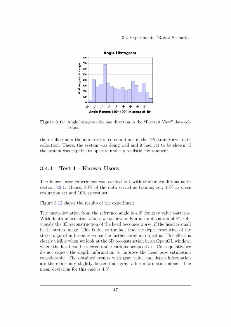
Figure 3.11 shows the histogram of the recorded pan angles in the imagesequences. Unlike for the “Portrait View” data collection the histogramvalues for the different angle ranges are pretty much the same. This is due tothe pointing gestures the users executed. The targets the users had to pointat, were spread equally in the room. Since people tend to look at the targetthey are pointing to, the head orientations were also distributed equally.
3.4 Experiments “Robot Scenario”
Under the new conditions in the “Robot Scenario” two experiments have beenperformed. One experiment evaluated the neural network’s performance onknown users, the other on unknown users.
The goal of these experiments was to compare the system’s performance to
46
3.4 Experiments “Robot Scenario”
Figure 3.11: Angle histogram for pan direction in the “Portrait View” data col-lection
the results under the more restricted conditions in the “Portrait View” datacollection. There, the system was doing well and it had yet to be shown, ifthe system was capable to operate under a realistic environment.
3.4.1 Test 1 - Known Users
The known user experiment was carried out with similar conditions as insection 3.2.1. Hence, 80% of the data served as training set, 10% as crossevaluation set and 10% as test set.
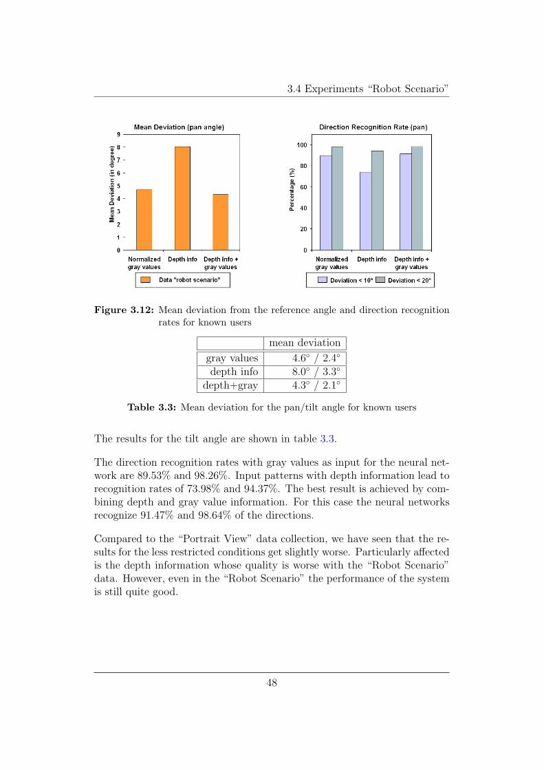
Figure 3.12 shows the results of the experiment.
The mean deviation from the reference angle is 4.6◦ for gray value patterns.With depth information alone, we achieve only a mean deviation of 8◦. Ob-viously the 3D reconstruction of the head becomes worse, if the head is smallin the stereo image. This is due to the fact that the depth resolution of thestereo algorithm becomes worse the farther away an object is. This effect isclearly visible when we look at the 3D reconstruction in an OpenGL window,where the head can be viewed under various perspectives. Consequently, wedo not expect the depth information to improve the head pose estimationconsiderably. The obtained results with gray value and depth informationare therefore only slightly better than gray value information alone. Themean deviation for this case is 4.3◦.
47
3.4 Experiments “Robot Scenario”
Figure 3.12: Mean deviation from the reference angle and direction recognitionrates for known users
mean deviation
gray values 4.6◦ / 2.4◦
depth info 8.0◦ / 3.3◦
depth+gray 4.3◦ / 2.1◦
Table 3.3: Mean deviation for the pan/tilt angle for known users
The results for the tilt angle are shown in table 3.3.
The direction recognition rates with gray values as input for the neural net-work are 89.53% and 98.26%. Input patterns with depth information lead torecognition rates of 73.98% and 94.37%. The best result is achieved by com-bining depth and gray value information. For this case the neural networksrecognize 91.47% and 98.64% of the directions.
Compared to the “Portrait View” data collection, we have seen that the re-sults for the less restricted conditions get slightly worse. Particularly affectedis the depth information whose quality is worse with the “Robot Scenario”data. However, even in the “Robot Scenario” the performance of the systemis still quite good.
48
3.4 Experiments “Robot Scenario”
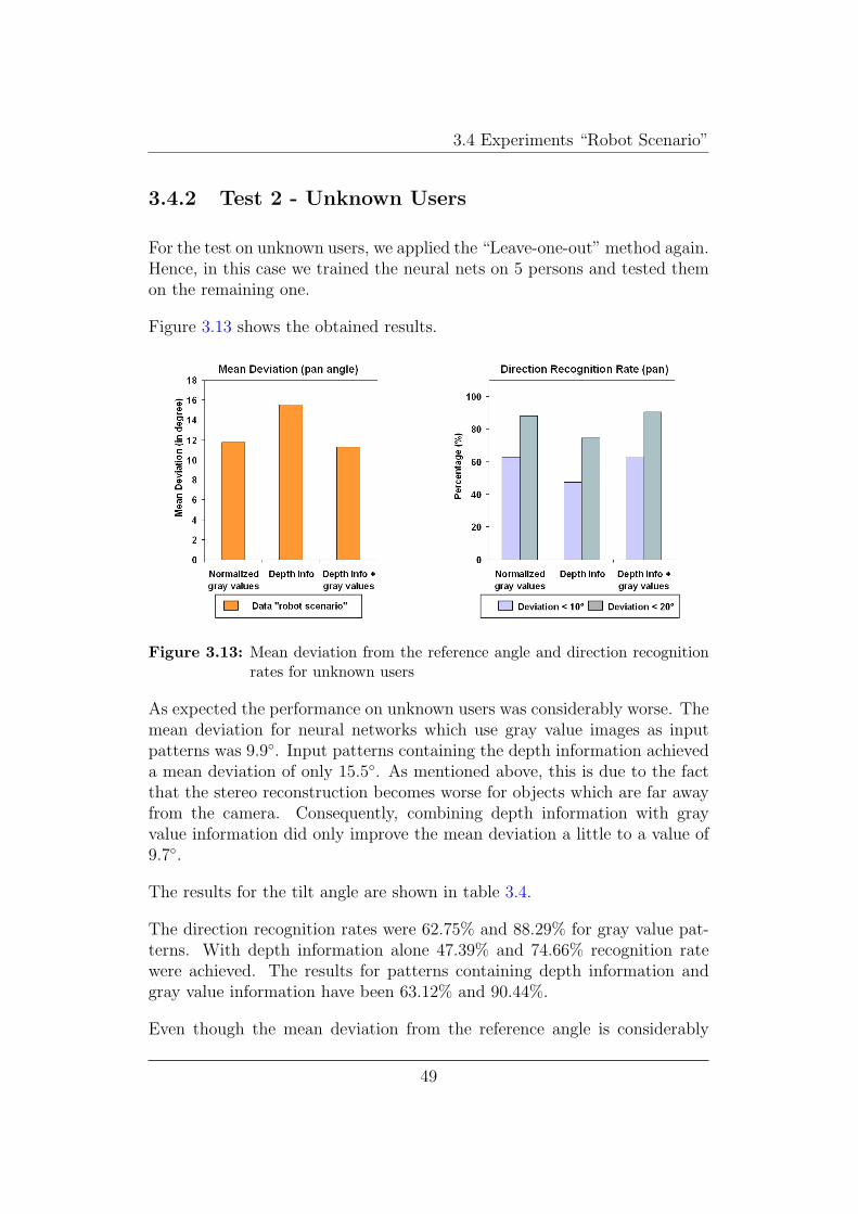
3.4.2 Test 2 - Unknown Users
For the test on unknown users, we applied the “Leave-one-out” method again.Hence, in this case we trained the neural nets on 5 persons and tested themon the remaining one.
Figure 3.13 shows the obtained results.
Figure 3.13: Mean deviation from the reference angle and direction recognitionrates for unknown users
As expected the performance on unknown users was considerably worse. Themean deviation for neural networks which use gray value images as inputpatterns was 9.9◦. Input patterns containing the depth information achieveda mean deviation of only 15.5◦. As mentioned above, this is due to the factthat the stereo reconstruction becomes worse for objects which are far awayfrom the camera. Consequently, combining depth information with grayvalue information did only improve the mean deviation a little to a value of9.7◦.
The results for the tilt angle are shown in table 3.4.
The direction recognition rates were 62.75% and 88.29% for gray value pat-terns. With depth information alone 47.39% and 74.66% recognition ratewere achieved. The results for patterns containing depth information andgray value information have been 63.12% and 90.44%.
Even though the mean deviation from the reference angle is considerably
49
3.4 Experiments “Robot Scenario”
mean deviation
gray values 15.5◦ / 6.3◦
depth info 11.0◦ / 5.7◦
depth+gray 9.7◦ / 5.6◦
Table 3.4: Mean deviation for the pan/tilt angle for unknown users
higher. The estimated angles can still give a robot a good hint on where aperson is looking. Recognition rates of up to 90% seem to make the methodapplicable in practice (see also chapter 4.1).
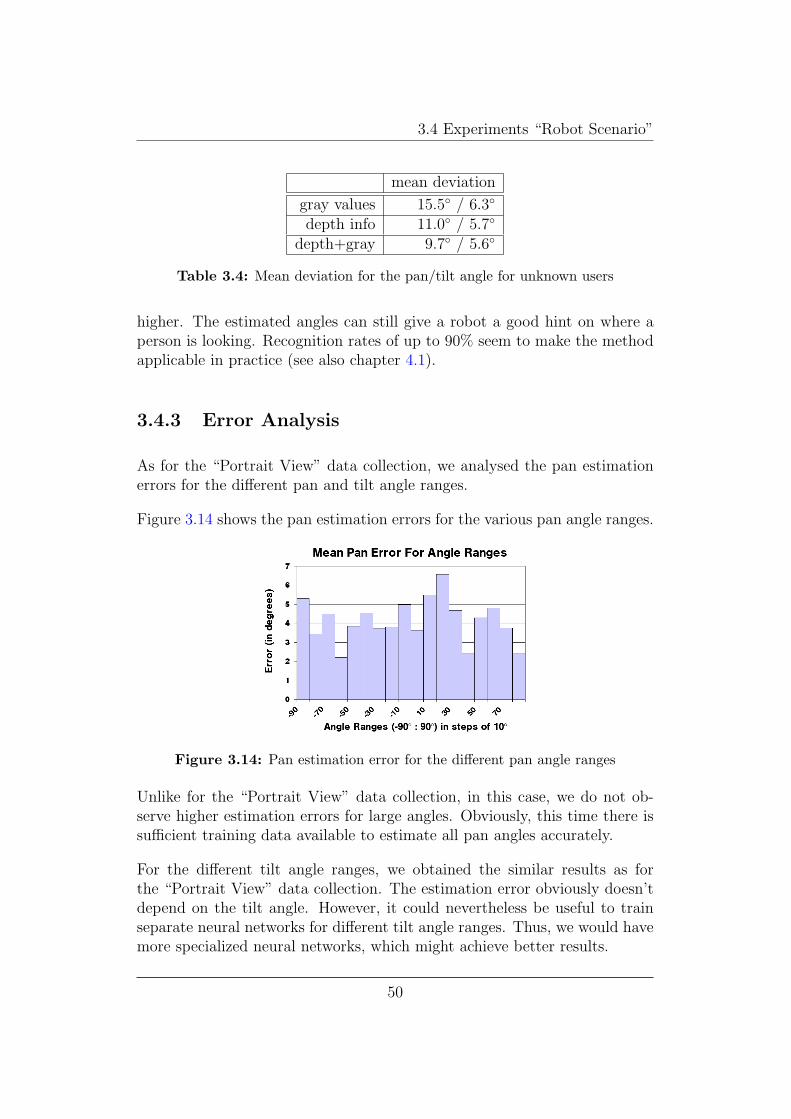
3.4.3 Error Analysis
As for the “Portrait View” data collection, we analysed the pan estimationerrors for the different pan and tilt angle ranges.
Figure 3.14 shows the pan estimation errors for the various pan angle ranges.
Figure 3.14: Pan estimation error for the different pan angle ranges
Unlike for the “Portrait View” data collection, in this case, we do not ob-serve higher estimation errors for large angles. Obviously, this time there issufficient training data available to estimate all pan angles accurately.
For the different tilt angle ranges, we obtained the similar results as forthe “Portrait View” data collection. The estimation error obviously doesn’tdepend on the tilt angle. However, it could nevertheless be useful to trainseparate neural networks for different tilt angle ranges. Thus, we would havemore specialized neural networks, which might achieve better results.
50

3.4 Experiments “Robot Scenario”
We conclude that the neural network’s head pose estimation is almost equallyaccurate for all pan and tilt angle ranges. Obviously the neural network isable learn the head orientations well even if the rotation angles are large.
3.4.4 Filtering
During the analysis of the estimated rotation angles, we observed that theneural networks pose estimates are rather noisy (see figure 3.15).
Figure 3.15: Estimation of the rotation angles is rather noisy
In order to further improve the estimation results, it therefore seemed to beuseful to filter the neural network output with some filter technique. Kalmanfilters are widely used for such tasks and have proven excellent performance.Given the nature of our application, the smooth movement of head in time,Kalman filters should perform well on our application data, too.
The Kalman filter estimates the state xk ∈ Rn of process, that is governedby a linear stochastic difference equation:
xk = Axk−1 + wk−1 (3.1)
with a measurement z ∈ Rm that is
zk = Hxk + vk (3.2)
The wk and vk represent the process and measurement noise. For a moredetailed description of the Kalman filter, please refer to appendix C.
51

3.4 Experiments “Robot Scenario”
Hence, in order to implement a Kalman filter for our application, we have todefine a state vector xk, a process matrix A, a measurement vector zk anda measurement matrix H. Moreover, we have to know something about thenature of the measurement and process noise wk and vk.
Obviously, in our application the pan angle at time step k can be calculatedfrom the pan angle at time step k − 1 and the rotation velocity at timestep k − 1. Consequently, we can define the state of the process by a two-dimensional vector consisting of the pan angle nk and the rotation velocitylk.
Equation 3.1 yields in this case:
xk =
(nk
lk
)= Axk−1 + wk−1 =
(1 dt
a21 a22
) (nk−1
lk−1
)+ wk−1 (3.3)
with dt the time difference between time step k and time step k − 1.
With the values for a21 and a22 we could model additional velocity changes.However, since we know nothing about a person’s behavior a modeling ofthese parameters isn’t possible. It is therefore assumed that the velocity isconstant. We obtain: 1
A =
(1 dt0 1
)(3.4)
A measurement in our application consists solely of the angle output of the
neural network. H is therefore the simple 1× 2 matrix
(10
).
For applying the predictor-corrector algorithm of the Kalman filter (see ap-pendix C.2), what still needs to be determined are the covariance matricesQ and R of the process and measurement noise.
The measurement error covariance may be calculated by taking some sam-ple measurements. In our application, the measurements correspond to theoutput of the neural network. Since, we also have the real head orientationsfrom our magnetic sensor, we can calculate the measurement error covarianceeasily from our data.
The process noise is somewhat more complicated, since the user may move hishead arbitrarily fast or slow. However, we can deduce a mean process noisefrom our recorded data. In this case, the filter achieves worse performance,if a user moves for example too fast.
52
3.4 Experiments “Robot Scenario”
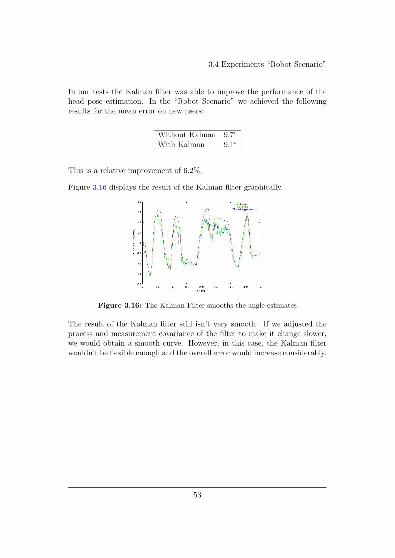
In our tests the Kalman filter was able to improve the performance of thehead pose estimation. In the “Robot Scenario” we achieved the followingresults for the mean error on new users:
Without Kalman 9.7◦
With Kalman 9.1◦
This is a relative improvement of 6.2%.
Figure 3.16 displays the result of the Kalman filter graphically.
Figure 3.16: The Kalman Filter smooths the angle estimates
The result of the Kalman filter still isn’t very smooth. If we adjusted theprocess and measurement covariance of the filter to make it change slower,we would obtain a smooth curve. However, in this case, the Kalman filterwouldn’t be flexible enough and the overall error would increase considerably.
53

Chapter 4
Head Pose Estimation inApplications
4.1 The Real-Time System
Real-time capability is one of the crucial points in computer vision. Inhuman-computer interaction, the estimation of head pose only makes sense,if the robot can immediately respond to it and thus if the estimation can bedone in real-time.
In order to prove the practicability of our approach, we implemented a real-time system of for the head pose estimation technique. In our tests, weachieved calculating 10 frames per second with a resolution of 320x240 pixels(Pentium 4, 2, 8 GHz). This is due to the fact, that once neural networks aretrained, they are extremely fast in computation. The activation levels of theinput patterns have simply to be propagated through the three layers of thenetwork. Face tracking with the color-based technique presented in section2.3 is rather fast as well. Taking skin color as selection criterion restricts thesearch space for algorithm considerably. The only issue for our system is thecalculation of the depth information. The stereo algorithm is computationalexpensive and restricts the frame rate considerably.
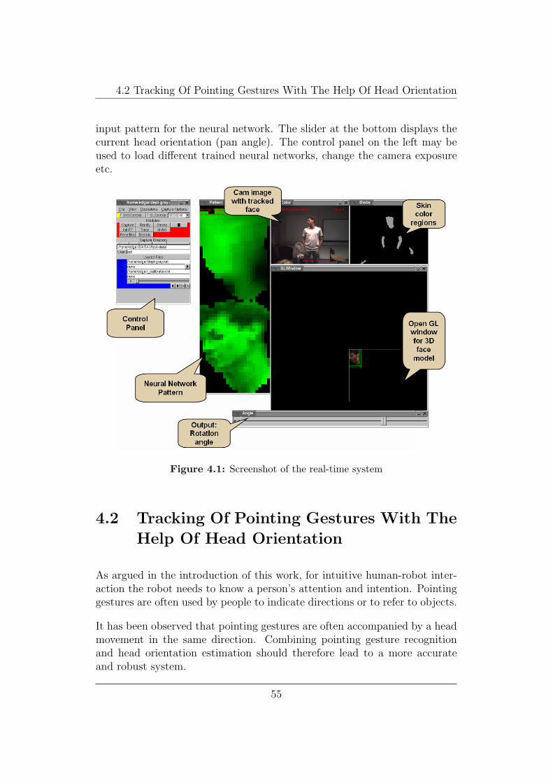
Figure 4.1 shows a screenshot of the real-time system. The two small windowsin the upper right corner display one of the current camera images and theskin color regions found in it. The windows below and left of these windowsshow the 3D reconstruction of the found head and the subsequently calculated
54
4.2 Tracking Of Pointing Gestures With The Help Of Head Orientation
input pattern for the neural network. The slider at the bottom displays thecurrent head orientation (pan angle). The control panel on the left may beused to load different trained neural networks, change the camera exposureetc.
Figure 4.1: Screenshot of the real-time system
4.2 Tracking Of Pointing Gestures With The
Help Of Head Orientation
As argued in the introduction of this work, for intuitive human-robot inter-action the robot needs to know a person’s attention and intention. Pointinggestures are often used by people to indicate directions or to refer to objects.
It has been observed that pointing gestures are often accompanied by a headmovement in the same direction. Combining pointing gesture recognitionand head orientation estimation should therefore lead to a more accurateand robust system.
55

4.2 Tracking Of Pointing Gestures With The Help Of Head Orientation
Nickel and Stiefelhagen [NS2003] proposed a framework to track pointinggestures with hidden markov models. In their setup, they marked severaltargets, at which a user had to point (see figure 4.2). They computed thenumber of pointing gestures, which have been recognized. Moreover theycalculated the difference of the target angle to the angle of the recognizedgesture (angle error).
1
23
45
6
7
8
-2-1
01
2x [m]
-1
0
1
2
3
4
z [m]
0
1
2
3
y [m]
Targets Setup
Figure 4.2: Targets and setup of the gesture recognition system (images takenfrom [NS2003])
In order to improve their recognition results, head orientation informationwas added to the feature vector. Table 4.1 shows the obtained results.
Recall Precision angle errorNo Head-Orientation 79.8% 73.6% 19.4◦
Sensor Head-Orientation 78.3% 86.3% 16.8◦
Estimated Head-Orientation 78.3% 87.1% 16.9◦
Table 4.1: Performance of gesture recognition with and without including head-orientation to the feature vector
The pointing gesture recognition without any head orientation informationachieved a recall of 79.8%. The precision was 73.6% and the average errorfrom the target angle to the estimated pointing angle was 19.4◦.
When head orientation information from a magnetic sensor was added, therecall decreased by 1.5%. However, the precision increased significantly byan absolute 12.6%. Moreover the angle error was only 16.8◦. Obviously, thehead orientation information does improve the recognition performance ofthe pointing gesture system.
56

4.2 Tracking Of Pointing Gestures With The Help Of Head Orientation
Surprisingly, even though the head orientations from the magnetic sensor aremore accurate than the ones estimated with the neural network, the resultsimprove slightly. The precision increases by 0.8%.
It can be concluded that the visual estimation of head orientation is capableof improving the results of the pointing gesture recognition.
57

Chapter 5
Conclusion and Future Work
In this work, a new approach to head pose estimation was presented. Itis based on neural networks and uses depth information to improve estima-tion results. The approach was evaluated under various conditions includingthe performance on known, unknown user and under lighting fluctuations.Furthermore different scenarios have been considered: A “Portrait View”scenario where the user only moves his head and a “Robot Scenario” whichis more realistic and allows the user to move around freely.
The results obtained with the proposed approach are rather promising. De-pending on the environments, a mean deviation between 3.2◦ and 9.7◦ hasbeen achieved. Direction recognition rates range between 90.44% and 99.7%for the various scenarios, if a deviation of 20◦ is allowed. The accuracy seemsto be suitable for pratical applications.
We have seen, that stereo information helps improving the estimation of thehead orientation angles considerably. Moreover it improves the robustness ofthe system under changing lighting conditions. Kalman Filtering can furtherimprove the obtained results.
We proved the practicability of the approach by implementing a real-timehead pose estimation system which operates at 10 frames per second. Theimplemented system has proven to be enhance human-robot interaction. Ithas, for example, been used to improve the results of a pointing gesturerecognition system by adding the estimated head pose to the feature vector[NSS2004].
58
Even though adding stereo information has improved the robustness of thesystem significantly, the performance still degrades noticeably under newlighting conditions. Here further work is necessary.
Further improvements of this approach could be obtained incorporating in-formation about the tilt angle into the neural network for estimating the panangle. This could, for example, be accomplished by training three differentpan estimation networks for large, average and small tilt angles. A neuralnetwork trained on the tilt angle could be used to determine which networkto use.
Other enhancements could be made in the preprocessing stage. By applyingtechniques like principal component analysis, the dimensionality of the inputpatterns could be reduced and important information extracted. This shouldlead to better recognition results especially for unknown users.
Speed improvements could be achieved by calculating depth information onlyon a small window around the current position of the head. Only in this areadepth information is necessary for head pose estimation. This could lead toreal-time capability even on higher resolutions.
59

Appendix A
Neural Networks
A.1 Introduction To Neural Networks
Artificial Neural Networks are inspired by the way biological nervous systems,such as the brain, work. They are composed of a large number of highlyinterconnected processing elements (neurones) working together to solve aspecific problem.
Until now, neural networks have been applied to a great number of problems.This is due to the fact that neural networks are a very versatile technique.They have been particularly popular in the area of pattern recognition andimage analysis.
A.2 Advantages Of Neural Networks
Neural networks have the remarkable ability to derive meaning from compli-cated or imprecise data. They may be used to extract patterns and detecttrends that are too complex to be noticed by either humans or other com-puter techniques. A trained neural network can generalize, meaning that itis not only able to reproduce what it has been trained, but also to interpolatenew results.
Other advantages include [SS1996]:
60

A.3 Building Blocks Of Neural Networks
• Adaptive learning: An ability to learn how to do tasks based on thedata given for training or initial experience.
• Self-Organization: A neural network can create its own organisationor representation of the information it receives during learning time
• Real Time Operation: Neural network computations may be carriedout in parallel, and special hardware devices are being designed andmanufactured which take advantage of this capability.
• Fault Tolerance via Redundant Information Coding: Partialdestruction of a network leads to the corresponding degradation of per-formance. However, some network capabilities may be retained evenwith major network damage.
A.3 Building Blocks Of Neural Networks
A neural network consists of units (neurones) and links or connections be-tween these units. In analogy to activation passing in biological neurons,each unit receives the output of its prior units as input.
Figure A.1 shows a small sample network.
Figure A.1: A simple neural network
The direction of a connection shows the direction in which the activationsare passed. Each connection has an associated weight. The effect of a uniton its successor is influenced by this weight. Negative values decrease theactivity of the succeeding units, positive values enhance it.
Depending on the function of a unit, we distinguish three different types.Units which have no predecessors are called input units. Their activation
61

A.3 Building Blocks Of Neural Networks
levels are set by the application/problem data itself or are fixed (for exam-ple, special “ON” units). Units whose output represents a part of the resultof a neural network computation are called output units. For classificationproblems there is usually one output unit for each possible class. All remain-ing units are called hidden units, since their inputs can not be directly setand their outputs not directly observed.
The actual information processing within the units is accomplished by theactivation and the output function which are associated with each unit.
First, the activation function computes the net input from the weighted out-puts of the prior units. Then, the new activation level of the unit is calcu-lated. The general formula for an activation function is:
aj(t + 1) = fact(netj(t), aj(t), θj) (A.1)
where:
aj(t) activation level of unit j at time/step tnetj(t) net input in unit j at time/step tθj threshold (bias) of unit j
The net input netj(t) is computed with
netj(t) =∑
i
wijoi(t) (A.2)
where:oi(t) output of unit i at time/step twij weight of the connection between unit i and j
The output function takes the activation value as input and subsequentlycomputes the output of the unit. The general formula is:
oj(t) = fout(aj(t)) (A.3)
with aj(t) and oj(t) as defined above.
In the literature, there often doesn’t exist both an activation and an outputfunction for a neural network unit. In this case there is only one process-
62

A.4 Learning With Neural Networks
ing function per unit defined, which is also called activation function. Thisfunction receives the net input as input parameter.
A.4 Learning With Neural Networks
A.4.1 Linear Discriminant Functions and Single-LayerNetworks
Single-layer neural networks consist of a single layer of adaptive weights.They can be used to distinguish two or more classes with linear decisionboundaries.
Consider a linear discriminant function y of the form of A.4, which separatestwo classes C1 and C2.
y(x) = wT x + w0, x ∈ Rd (A.4)
y(x) = 0 represents a hyperplane in the d-dimensional space Rd. The vectorw is chosen to fulfill the following formula:
y(x) =
{< 0 if x ∈ C1
> 0 if x ∈ C2
Such a decision boundary can be modeled with a simple neural network asshown in figure A.2 (left) in the following manner. The weights of the networkare defined as the values of the vector w, the activation function fact of theoutput unit is defined as y and the output function as the identity.
Figure A.2: Single-layer neural networks
63
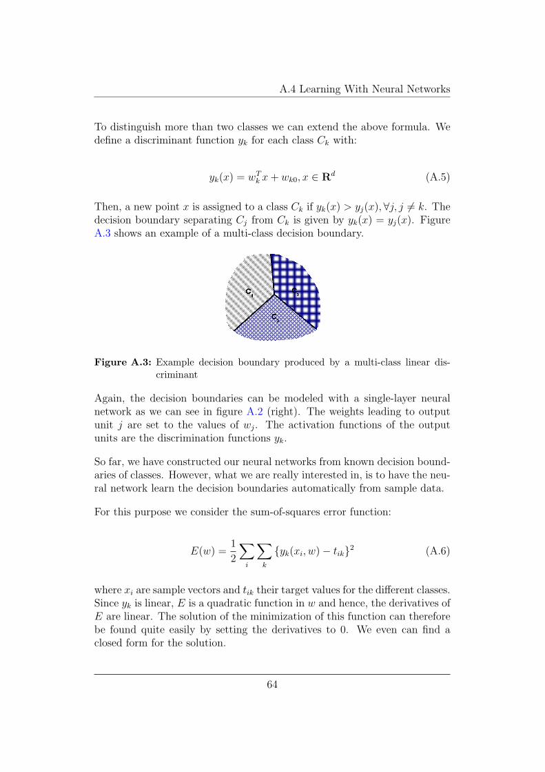
A.4 Learning With Neural Networks
To distinguish more than two classes we can extend the above formula. Wedefine a discriminant function yk for each class Ck with:
yk(x) = wTk x + wk0, x ∈ Rd (A.5)
Then, a new point x is assigned to a class Ck if yk(x) > yj(x),∀j, j 6= k. Thedecision boundary separating Cj from Ck is given by yk(x) = yj(x). FigureA.3 shows an example of a multi-class decision boundary.
Figure A.3: Example decision boundary produced by a multi-class linear dis-criminant
Again, the decision boundaries can be modeled with a single-layer neuralnetwork as we can see in figure A.2 (right). The weights leading to outputunit j are set to the values of wj. The activation functions of the outputunits are the discrimination functions yk.
So far, we have constructed our neural networks from known decision bound-aries of classes. However, what we are really interested in, is to have the neu-ral network learn the decision boundaries automatically from sample data.
For this purpose we consider the sum-of-squares error function:
E(w) =1
2
∑i
∑k
{yk(xi, w)− tik}2 (A.6)
where xi are sample vectors and tik their target values for the different classes.Since yk is linear, E is a quadratic function in w and hence, the derivatives ofE are linear. The solution of the minimization of this function can thereforebe found quite easily by setting the derivatives to 0. We even can find aclosed form for the solution.
64
A.4 Learning With Neural Networks
Consequently, for arbitrary linear decision boundaries in Rd we can findweights w such that a neural network with the activation functions yk for theoutput units, can classify all vectors correctly.
When considering different error functions or a non-linear function as activa-tion function, such an explicit solution is not possible any more. However, ifthe activation function is differentiable, we can still calculate the derivativesof the error function E. These derivatives can be used to perform a gradientdescent to find a suitable solution.
We may adopt the following procedure. We begin with an initial guess ofthe weights w. Subsequently, we move a small distance in w-space in thedirection where E decreases the most rapidly. By iterating this process, wecreate a sequence of weights wr whose components may be calculated withthe following formula:
wr+1kj = wr
kj − η∂E
∂wkj
∣∣∣∣wr
(A.7)
where η is a small positive number called learning rate. Under suitable condi-tions the values of w will converge to a point where E is minimal. The choiceof η is rather important, since low learning rates lead to a slow convergence,whereas high learning rates may lead to oscillation and divergence.
A.4.2 The Perceptron
A perceptron is a single-layer neural network with one output unit. To im-prove the performance the perceptron has a layer of fixed processing elementsto transform the raw data. These processing elements can be considered asthe basis function of a generalized linear discriminant.
Consequently, the output of the perceptron is given by
y = g
( ∑j
wjφj(x))
= g(wT φ) (A.8)
where φ is the vector of activations. The activation function of the output isdefined by a threshold function of the form:
65
A.4 Learning With Neural Networks
g(a) =
{−1 if a < 0+1 if a ≥ 0
(A.9)
For the perceptron often a continuous, piecewise-linear error function calledperceptron criterion is considered. It is a measure for the number of misclas-sifications the perceptron has performed. Suppose that with each activationvector φn we obtain an associated target value tn. With tn = −1 if φn belongsto class C1 and tn = +1 if phin belongs to class C2. Then the perceptroncriterion Eperc can be written as:
Eperc(w) = −∑
φn∈M
wT (φntn) (A.10)
with M the set of vectors φn which are misclassified by the current weightvector w.
Now, if we apply the pattern-by-pattern gradient descent rule from equationA.7, we obtain the following learning rule:
wr+1j = wr
j + ηφnj t
n (A.11)
Hence, we have a very simple learning algorithm, that can be summarized asfollows. Cycle through all input patterns in the training set with the currentweights. If a pattern is misclassified simply add/subtract the pattern vectormultiplied by η to the weights.
There is an interesting result which states that, for any data set which islinearly separable, the learning rule is guaranteed to find a solution in afinite number of steps. This property is known as the perceptron convergencetheorem.
A.4.3 Multi-Layer Networks
As we have seen, single-layer networks have the limitation, that classes haveto be linearly separable. Any problem requiring non-linear decision bound-aries can not be classified by these networks. This is for example true for theXOR problem A.4.
66

A.4 Learning With Neural Networks
� �� �� �� � � �� �
� �� �
class 1 class 2
� �� �� �� �� �� �
� �� �� �� �� � �� � �
� � �� � �� � �
Figure A.4: The classes in the XOR problem are not linearly separable and thusa single-layer network cannot classify the elements correctly
Now, we want to have a look at the capabilities of multi-layer networks. Weconcentrate on networks consisting of successive layers of adaptive weights.These networks are easier to analyze theoretically than more general topolo-gies. Moreover they can be implemented more efficiently in software or hard-ware. This kind of network can be viewed as a transformation of the in-put data by successive single-layer networks. Meaning that the output ofone single-layer network is processed by the succeeding single-layer network.Therefore these networks are also called feed-forward networks. Figure [REF-ERENCE], for example, shows a two-layer network, which can solve the XORproblem.
Figure
It can be shown that even neural networks with two-layer of adaptive weightsare capable of approximating an arbitrary continuous mapping from onefinite-dimensional space to another, provided the number of hidden units issufficiently large. For the classification problem, we can obtain an impor-tant corollary of this property. Two-layer networks with sigmoidal activationfunctions can approximate any decision boundary to arbitrary accuracy (see[Krei1991]). Thus, such networks also provide universal non-linear discrimi-nation functions.
Next to this theoretical result, feed-forward networks are used because thereexists a powerful and computational efficient method for finding the deriva-tives of an error function with respect to the weights. Provided that, theactivation function are differentiable. This method can be used to train theneural network and is called error back-propagation.
67

A.4 Learning With Neural Networks
Error-Backpropagation
For the error-backpropagation, we consider each training pattern separately.The error function E is defined as:
E =∑
n
En (A.12)
where En is the error function for the pattern with index n. We supposethat En is differentiable for all n.
The unit input is in the following denoted by aj and computed as we alreadyhave seen above:
aj =∑
i
wjizi (A.13)
with zi the activations of the predecessing units, which are calculated fromtheir own unit inputs as follows:
zj = g(aj) (A.14)
where g may be a non-linear activation function.
For each pattern, we now suppose that we have supplied the correspondinginput vector to the neural network and calculated the activations of all hiddenand output units by successive application of equation A.13 and A.14. Thisprocess is called forward propagation, since the activations are calculatedfrom one layer to the next.
Our goal is to find a procedure for evaluating the derivatives of En withrespect to the weights. Since En depends on the weight wji only via the unitinput aj, we can apply the chain rule for partial derivatives:
∂En
∂wji
=∂En
∂aj
∂aj
∂wji
(A.15)
Using A.13, we can write:
68

A.4 Learning With Neural Networks
∂aj
∂wji
= zi (A.16)
Thus, in order to evaluate the derivative of En we only have to calculate ∂En
∂aj
for each hidden and output unit in the network.
For the output units the evaluation can be done easily using equation A.14:
∂En
∂ak
= g ′(ak)∂En
∂yk
(A.17)
The values on the right hand side of the equation are known from the defi-nition of the activation and error function as well as from the forward prop-agation phase.
For the hidden units we again make use of the chain rule for partial deriva-tives:
∂En
∂aj
=∑
k
∂En
∂ak
∂ak
∂aj
(A.18)
where the sum runs over all units with index k to which unit j sends aconnection.
By making use of the equations A.13 and A.14 we obtain the following back-propagation formula:
δj =∂En
∂aj
= g ′(aj)∑
k
wkj∂En
∂ak
(A.19)
Consequently, now we can evaluate the derivatives of En with respect to theweights with the following algorithm:
1. Apply an input pattern to the network and forward propagate theactivations through all layers
2. Evaluate the δk for all output units
69

A.5 Generalization Of Neural Networks
3. Back-propagate the δ’s using the backpropagation formula
4. Use the resulting δ’s to calculate the derivatives of En and E
To perform a learning step, what still needs to be done is alter the weightswith a gradient descent technique. For example:
∆wji = −η∂En
∂wji
(A.20)
with η the learning rate.
There exist a number of other learning techniques for neural networks. Quick-prop and Rprop, for example, try to improve convergence speed for the learn-ing algorithm. It is not intended to cover these techniques in this work. Fora detailed description see [SNNSRef].
A.5 Generalization Of Neural Networks
Neural networks have the ability to generalize. This means that a trainedneural network can classify data that has never been seen before. In realworld applications developers normally have only a small part of all possiblepatterns. To reach best generalization, the data set is generally split intothree parts:
• Training set
• Cross evaluation set
• Test set
the training set is used to train the neural network. Backpropagation or otherlearning techniques is used to minimize the error during training. The crossevaluation set is used to determine the performance of the neural network onpatterns, which are unknown to the network. This is a measure of whetherthe network generalizes well. Finally, the test set is used for checking theover all performance of the neural network.
70

A.5 Generalization Of Neural Networks
Usually during training the performance of the network is continuously testedon the cross evaluation set. If the error on the cross evaluation set reachesa minimum the training is stopped. The error on the training set may stilldecrease if further training is applied. However, this is the point where theneural network is considered to generalize best. Remember, our goal hasn’tbeen to obtain the best possible results on the training set, but to obtain aneural network which performs well on all possible data. If we would continueto train the neural network, we would see an effect called over-fitting, meaningthat the general performance of the network decreases.
Figure A.5 shows an example of a typical error development during neuralnetwork training.
Error on training set Error on cross evaluation set
Training cycles
Err
or
Figure A.5: Development of the error during neural network training
A crucial point when dealing with neural network is the availability of train-ing data. The more units the neural network contains, the more trainingdata is needed to achieve good performance. Next to the quantity of train-ing data, it is important that there are enough training patterns for eachclass we want to classify.
71

Appendix B
Pattern-Based Face Detection
This chapter describes the face detection technique developed by Viola andJones [VJ2001], which is used in our system to find a skin color region.
The technique classifies images based on the value of simple features. Fea-tures have the advantage that the can act to encode ad-hoc domain knowl-edge, which might be difficult to learn from the image data itself. Specifi-cally, four kinds of features are used in this algorithm: horizontal and verticaltwo-rectangle features, a vertical three-rectangle feature and a four-rectanglefeature (see figure B.1).
Figure B.1: Example rectangle features shown relative to a detection window
The value of a feature is computed by summing up all pixels in the gray areasand calculating the difference to the pixels in the white areas.
In order to compute these features efficiently, a so-called integral image isused. For an image i(x, y) the integral image ii is defined by:
72
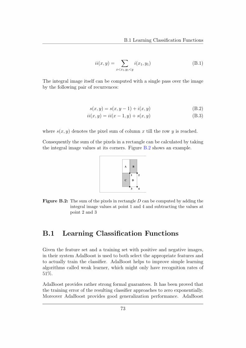
B.1 Learning Classification Functions
ii(x, y) =∑
x<x1,y1<y
i(x1, y1) (B.1)
The integral image itself can be computed with a single pass over the imageby the following pair of recurrences:
s(x, y) = s(x, y − 1) + i(x, y) (B.2)
ii(x, y) = ii(x− 1, y) + s(x, y) (B.3)
where s(x, y) denotes the pixel sum of column x till the row y is reached.
Consequently the sum of the pixels in a rectangle can be calculated by takingthe integral image values at its corners. Figure B.2 shows an example.
BA
C D
1 2
3 4
Figure B.2: The sum of the pixels in rectangle D can be computed by adding theintegral image values at point 1 and 4 and subtracting the values atpoint 2 and 3
B.1 Learning Classification Functions
Given the feature set and a training set with positive and negative images,in their system AdaBoost is used to both select the appropriate features andto actually train the classifier. AdaBoost helps to improve simple learningalgorithms called weak learner, which might only have recognition rates of51%.
AdaBoost provides rather strong formal guarantees. It has been proved thatthe training error of the resulting classifier approaches to zero exponentially.Moreover AdaBoost provides good generalization performance. AdaBoost
73

B.1 Learning Classification Functions
helps finding a small set of good classification functions which have significantvariety nevertheless.
In their face detection algorithm these classification functions or weak learn-ers correspond to finding a rectangle features and a threshold, which canperform the classification task with low error. The weak learners hj there-fore can be written in the following manner:
hj(x) =
{1 ±fj(x) < σj
0 otherwise(B.4)
with x a detection window, fj a rectangle feature, and σj a threshold value.
The boosting algorithm based on these weak learners works as follows (see[VJ2001]):
• Given example images (x1, y1), . . . , (xn, yn) where yi = 0, 1 for negativeand positive examples respectively.
• Initialize weights w1,i = 12m
, 12l
for yi = 0, 1 respectively, where m and lare the number of negatives and positives
• For t = 1, . . . , T :
1. Normalize the weights,
wt,i =wt,i∑n
j=1 wt,j
(B.5)
so that wt is a probability distribution.
2. For each feature j train a classifier hj which is restricted to usinga single feature. The error is evaluated with respect to wt, ej =∑
i wi|hj(xi)− yi|.3. Choose the classifier ht with the lowest error et.
4. Update the weights:
wt+1,i = wt,iβ1−eit (B.6)
where ei = 0 if example xi is classified correctly, ei = 1 otherwise,and βt = et
1−et.
74

B.1 Learning Classification Functions
• The final strong classifier is:
h(x) =
{1
∑Tt=1 αtht(x) ≥ 1
2
∑Tt=1 αt
0 otherwise(B.7)
where αt = log 1βt
.
Figure B.3 shows the first and the second features selected by the boostingalgorithm. The two-rectangle feature represents the fact, that eyes are darkerthen the upper cheeks. The three-rectangle feature compares the intensitiesin the eye regions to the intensity across the bridge of the nose.
Figure B.3: First and second features selected by AdaBoost (images taken from[VJ2001])
In order to improve detection performance, Viola and Jones implemented aso-called attentional cascade. The image windows pass through some kind ofdegenerated decision tree with a classifier at each node. The cascade helpsfiltering out a great number of images with the computation of a single orseveral simple classifiers. Only the image windows which pass all the cascadenodes are considered to be a face. For more details and experimental resultsplease refer to [VJ2001].
75
Appendix C
Discrete Kalman Filter
The Kalman filter has been subject of extensive research. It has been usedfor all kinds of applications where measurements of a continuous process wasnoisy and results had to be filtered.
The discrete Kalman filter addresses the general problem of estimating astate x ∈ Rn of a discrete-time controlled process. The underlying stochasticequation has the following form:
xk = Axk−1 + wk−1 (C.1)
where xk is the state of the process and at time k and wk the process noise.Apart from the process noise, the matrix A defines how a state xk is calculatedfrom its previous state.
A measurement z ∈ Rm is derived from a state k with:
zk = Hxk + vk (C.2)
where vk is the measurement noise. The matrix H computes the measurementvector from a state xk.
We assume the random variables wk, vk to be distributed normally withcovariance matrices Q and R:
76
C.1 Basic Kalman Filter Equations
p(w) ∼ N(0, Q) (C.3)
p(v) ∼ N(0, R) (C.4)
The measurement noise covariance R and the process noise covariance Qmight change with each time step of measurement. However we assume thematrices to be constant.
C.1 Basic Kalman Filter Equations
We define xpriork to be the a priori state estimate given the knowledge of
the process states prior to step k. Moreover, we define xposterk to be the a
posteriori state estimate given the knowledge of the process states prior tostep k and the measurement vector zk. The corresponding errors eprior
k andeposter
k are consequently:
epriork = xk − xprior
k (C.5)
eposterk = xk − xposter
k (C.6)
The a priori and a posteriori covariance matrices follow from epriork and
eposterk :
P priork = E[eprior
k epriork
T] (C.7)
P posterk = E[eposter
k eposterk
T] (C.8)
Now the Kalman filter equation can be derived from the above equations. Inthis equation, the a posteriori state xposter
k is computed from its correspondinga priori state xprior
k , as well as the weighted difference of the measurementvector zk and a measurement prediction Hxprior
k . We obtain the followingformula:
xposterk = xprior
k + K(zk −Hxpriork ) (C.9)
77
C.2 The Predictor-Corrector Process
The justification for this equation comes from the probabilistic origin of thefilter. For further details see [Jaco1993]. The difference (zk−Hxprior
k ) is calledmeasurement innovation and denotes the discrepancy between the predictedmeasurement and the actual measurement value. A difference value of 0means that the actual measurement is conform with the predicted one. Thea priori state estimate therefore has not to be updated.
The n×m matrix K in equation C.9 is chosen to minimize the a posteriorierror covariance P poster
k . The minimization can be accomplished by substitut-ing the Kalman filter equation into the definition of eposter
k and substitutingthis into the definition of P poster
k . Subsequently, the derivative of the traceof P poster
k with respect to K can be calculated and set to 0. We obtain theresulting matrix Kk for step k of the process:
Kk = P priork HT (HP prior
k HT + R)−1 (C.10)
Obviously, the more the measurement error covariance approaches 0 thelarger is the weight Kk gives to the measurement innovation. In this case, thea priori state estimate has to be updated to conform to the measurement.We also might say that we trust the actual measurement more than the apriori estimation. On the other hand, as the a priori estimate error covari-ance P prior
k decreases, the less weight is given to the measurement innovation.In that case, the a priori state estimation is rather good and can be trusted.Therefore the a priori estimation has only to be slightly changed.
C.2 The Predictor-Corrector Process
As might be imagined from the above section the Kalman filter estimatesthe process by using a form of feedback control also referred to as predictor-corrector approach. The filter predicts the state of the process at some stepk and then obtains feedback in form of a possibly noisy measurement.
As such, we define two groups of equations:
• time update equations (prediction step)
• measurement update equations (correction step)
78

C.2 The Predictor-Corrector Process
The specific equations for the time updates are:
xpriork = Axposter
k−1 (C.11)
P priork = AP poster
k−1 AT + Q (C.12)
Notice again, that these equations project the state and the covariance esti-mates forward from time step k − 1 to k.
For the measurement updates, we obtain:
Kk = P priork HT (HP prior
k HT + R)−1 (C.13)
xposterk = xprior
k + Kk(zk −Hxpriork ) (C.14)
P posterk = (I −KkH)P prior
k (C.15)
So, the first task during the measurement update is computing the matrix Kk
which minimizes the a posteriori error covariance (see section C.1). Subse-quently, the process is actually measured and the a posteriori state estimateis calculated with the help of this measurement. Finally, we need to computethe a posteriori covariance estimate for the next time update step.
Now, we can continue with another time update step. This two stage processis repeated from each time step k − 1 to k (see figure C.1).
MeasurementUpdate
Time Update
Figure C.1: Predictor-Corrector cycle of the Kalman filter
79
BIBLIOGRAPHY
Bibliography
[Adam2000] B. Adams et al., Humanoid robots: a new kind of tool, IEEEIntelligent Systems, pages 25-31, 2000
[Agah2001] A. Agah, Human interactions with intelligent systems: researchtaxonomy, Computers and Electrical Engineering,pages 71-107, 2001
[AHP1993] A. Azarbayejani, B. Horowitz and A. Pentland, Recursive esti-mation of structure and motion using the relative orientation constraint,Proceedings of the Computer Vision and Patteern Recognition Confer-ence, pages 70-75, 1993
[Bish2000] Christopher M. Bishop, Neural Networks for Pattern Recognition,Oxford University Press, 2000
[DTB2002] Darrell, T., Tollmar, K., Bentley, F., Checka, N., Morency, L.-P., Rahimi A., and Alice Oh, Face-responsive Interfaces: from DirectManipulation to Perceptive Presence, International Conference of Ubiq-uitous Computing, 2002
[Fitz2001] Paul Fitzpatrick, Head pose estimation without manual initializa-tion, AI Lab, MIT, Cambridge, USA, 2001
[HB1995] D. Heeger and J. Bergen, Pyramid-based texture analy-sis/synthesis, Proceedings of SIGGRAPH 1995, pages 229-238
[HH2002] Y. Huang, T. S. Huang, Facial Tracking with Head Pose Esti-mation in Stereo Vision, IEEE Int. Conference on Image Processing,Rochester, New York, US, September 22-25, 2002
[HRD1999] Michael Harville, Ali Rahimi, Trevor Darrell, Gaile G. Gordon,John Woodfill, 3D Pose Tracking with Linear Depth and BrightnessConstraints, ICCV 1999, pp. 206-213
80
BIBLIOGRAPHY
[HS1980] B.K.P. Horn and B.G. Schunck, Determining optical flow, AI Memo572, Massachusetts Institute of Technology, 1980
[Jaco1993] O. Jacobs, Introduction to Control Theory, 2nd Edition, OxfordUniversity Press, 1993
[Jahn1997] B. Jahne, Digitale Bildverarbeitung, Springer-Verlag, Berlin-Heidelberg, 4. Auflage, 1997
[KBS2000] Volker Kruger, Sven Bruns, Gerald Sommer, Efficient Head PoseEstimation with Gabor Wavelet Networks, Proc. British Machine VisionConference, Bristol, UK, Sept. 12-14, 2000.
[Koku2000] , A.B. Koku et al., Towards socially acceptable robots, Proceed-ings of 2000 IEEE International Conference on Systems, Man and Cy-bernetics, pages 894-899, 2000
[Kono1997] K. Konolige, Small Vision System: Hardware and Implementa-tion, IEEE Conference on Computer Eighth International Symposiumon Robotics Research, Hayama, Japan, 1997
[Krei1991] V. Y. Kreinovich, Arbitrary nonlinearity is sufficient to representall functions by neural networks: a theorem, Neural Networks 4 (3),pages 381-383, 1991
[Mats1999] , Y. Matsusaka et al., Multi-person conversation via multi-modalinterface - A robot who communicates with multi-user, Proc. Eurospeech99,pages 1723-1726, 1999
[Matt2002] Matteo Matteucci, ELeaRNT: Evolutionary Learning of RichNeural Network Topologies, Center for Automated Learning and Dis-covery, Technical Report, CMU-CALD-02-103, 2002
[MA2000] Yoshio Matsumoto, Tsukasa Ogasawara, Alexander Zelinsky, Be-havior Recognition Based on Head Pose and Gaze Direction Measure-ment, Proceedings of 2000 IEEE/RSJ International Conference on In-telligent Robots and Systems (IROS’2000), pp.2127-2132, 2000
[MC1993] B.S. Manjunath and R. Chellappa, A unified approach to boundaryperception: edges, textures and illusory contours, IEEE Trans. NeuralNetworks, 1993
[MRC2002] Louis-Philippe Morency, Ali Rahimi, Neal Checka, and TrevorDarrell, Fast stereobased head tracking for interactive environment, In
81

BIBLIOGRAPHY
Proceedings of the Int. Conference on Automatic Face and GestureRecognition, 2002.
[MZ2000] Yoshio Matsumoto, Alexander Zelinsky, An Algorithm for Real-time Stereo Vision Implementation of Head Pose and Gaze DirectionMeasurement, Proceedings of IEEE Fourth International Conference onFace and Gesture Recognition (FG’2000), pp.499-505, 2000
[NS2003] K. Nickel and R. Stiefelhagen, Pointing Gesture Recognition basedon 3D tracking of Face, Hands and Head Orientation, Fifth InternationalConference on Multimodal Interfaces, Vancouver, Canada, Nov. 5-7,2003
[Nick2003] Kai Nickel and Rainer Stiefelhagen, Detection and Tracking of3D-Pointing Gestures for Human-Robot-Interaction, Proceedings of theThird IEEE International Conference on Humanoid Robots - Humanoids2003, Karlsruhe, Germany, October 1-3, 2003
[NSS2004] Kai Nickel et al., Tracking Head and Hands for Pointing Ges-ture Recognition in a Human-Robot Interaction Scenario, submitted toInternational Conference on Automatic Face and Gesture Recognition(FG2004), Seoul, Korea, 2004
[Perz2001] D. Perzanowski et al., Building a multimodal human-robot inter-face, IEEE Intelligent Systems, pages 16-21,2001
[SA2000] Sangho Park, J.K. Aggarwal, Head Segmentation and Head Orien-tation in 3D Space for Pose Estimation of Multiple People, 4th IEEESouthwest Symposium on Image Analysis and Interpretation, p. 192,Austin, April 02-04, 2000
[SB2002] S. Srinivasan and K. L. Boyer, Head Pose Estimation Using ViewBased Eigenspaces, Intl. Conf. on Pattern Recognition, Quebec, 2002
[SM2002] Kenneth O. Stanley and Risto Miikkulainen, Efficient Evolutionof Neural Network Topologies, Proceedings of the 2002 Congress on Evo-lutionary Computation (CEC ’02). Piscataway, NJ: IEEE, 2002
[SNNSRef] Stuttgart Neural Network Simulator User Manual, Version 4.2
[SS1996] C. Stergiou and D. Siganos, Neural Networks, SURPRISE 96 Jour-nal, Department of Computing, Imperial College of Science Technologyand Medicine, London, 1996
82

BIBLIOGRAPHY
[Stie2002] Rainer Stiefelhagen, Tracking and Modeling Focus of Attention inMeetings, Dissertation, Universitat Karlsruhe, Fakultat fur Informatik,2002
[SYW2001] R. Stiefelhagen, J. Yang, A. Waibel, Tracking Focus of Attentionfor Human-Robot Communication, IEEE-RAS International Conferenceon Humanoid Robots - Humanoids 2001, November 22-24, 2001, Tokyo,Japan
[VJ2001] P. Viola and M. Jones Robust real-time object detection, TechnicalReport 2001/01, Compaq CRL, February 2001.
[WB2003] Greg Welch and Gary Bishop, An Introduction to the KalmanFilter, Technical Report TR 95-041 University of North Carolina atChapel Hill, 2003
[YLW1997] J. Yang, W. Lu and A. Waibel, Skin-Color Modeling and Adap-tion, Technical Report, School of Computer Science CMU-CS-97-146,CMU, USA, 1997
[YZ2001] R. Yang and Z. Zhang, Model-based Head Pose Tracking WithStereovision, In Proc. Fifth IEEE International Conference on Auto-matic Face and Gesture Recognition (FG2002), pages 255-260, Wash-ington, DC, May 20-21, 2002
[Zhan2000] Z. Zhang, A flexible new technique for camera calibration, IEEETransactions on Pattern Analysis and Machine Intelligence, 22(11):1330-1334, 2000
83