HAL Id: hal-01018885https://hal.archives-ouvertes.fr/hal-01018885

Submitted on 13 Mar 2015

HAL is a multi-disciplinary open accessarchive for the deposit and dissemination of sci-entific research documents, whether they are pub-lished or not. The documents may come fromteaching and research institutions in France orabroad, or from public or private research centers.

L’archive ouverte pluridisciplinaire HAL, estdestinée au dépôt et à la diffusion de documentsscientifiques de niveau recherche, publiés ou non,émanant des établissements d’enseignement et derecherche français ou étrangers, des laboratoirespublics ou privés.

Estimating human trajectories and hotspots throughmobile phone data

Sahar Hoteit, Stefano Secci, Stanislav Sobolevsky, Carlo Ratti, Guy Pujolle

To cite this version:Sahar Hoteit, Stefano Secci, Stanislav Sobolevsky, Carlo Ratti, Guy Pujolle. Estimating humantrajectories and hotspots through mobile phone data. Computer Networks, Elsevier, 2014, 64, pp.296-307. <hal-01018885>

Estimating Human Trajectories and Hotspots through

Mobile Phone Data

Sahar Hoteita, Stefano Seccia, Stanislav Sobolevskyb, Carlo Rattib,Guy Pujollea

aSorbonne Universities, UPMC Univ. Paris 06, UMR 7606, LIP6, F-75005, Paris,France (e-mails: sahar.hoteit@upmc.fr, stefano.secci@upmc.fr, guy.pujolle@upmc.fr)

bMIT Senseable City Laboratory, 77 Massachusetts Avenue Cambridge, MA 02139, USA(e-mails: stanly@mit.edu, ratti@mit.edu).

Abstract

Nowadays, the huge worldwide mobile-phone penetration is increasingly turn-ing the mobile network into a gigantic ubiquitous sensing platform, enablinglarge-scale analysis and applications. Recently, mobile data-based researchreached important conclusions about various aspects of human mobility pat-terns. But how accurately do these conclusions reflect the reality? To eval-uate the difference between reality and approximation methods, we studyin this paper the error between real human trajectory and the one obtainedthrough mobile phone data using different interpolation methods (linear, cu-bic, nearest interpolations) taking into consideration mobility parameters.Moreover, we evaluate the error between real and estimated load using theproposed interpolation methods. From extensive evaluations based on realcellular network activity data of the state of Massachusetts, we show that,with respect to human trajectories, the linear interpolation offers the bestestimation for sedentary people while the cubic one for commuters. Anotherimportant experimental finding is that trajectory estimation methods showdifferent error regimes whether used within or outside the “territory” of theuser defined by the radius of gyration. Regarding the load estimation error,we show that by using linear and cubic interpolation methods, we can findthe positions of the most crowded regions (“hotspots”) with a median errorlower than 7%.

Keywords: Mobility patterns, interpolation methods, trajectoryestimation, radius of gyration, hotspot estimation.

Preprint submitted to Elsevier June 4, 2014

1. Introduction

Human mobility and behavior pattern analysis has long been a prominentresearch topic for social scientists, urban planners, geographers, transporta-tion and telecommunication researchers, but the pertinence of results hasthus far been limited by the availability of quality data and suitable datamining techniques. Nowadays, the huge worldwide mobile-phone penetra-tion is increasingly turning the mobile network into a gigantic ubiquitoussensing platform, enabling large-scale analysis and applications.

In recent years, mobile data-based research reaches important conclusionsabout various aspects of human characteristics, such as human mobility andcalling patterns [1] [2] [3], virus spreading [4] [5], social networks [6] [7] [8],content consumption cartography [9], urban and transport planning [10] [11],network design [12].

Nevertheless, in such user displacement sampling data, a high uncertaintyis related to users movements, since available samples strongly depend on theuser-network interaction frequency. For instance, Call Data Records alonedo not provide a sufficiently fine granularity and accuracy, exhibiting a vastuncertainty about the periods when the user is not active, i.e., not com-municating. This represents an issue for applications or analyses assumingubiquitous and continuous user-tracking capability.

Some modeling techniques have been proposed in the literature to predictuser movement between two places.

Authors in [13] and [14] infer the top-k routes traversing a given locationsequence within a specified travel time from uncertain trajectories; they usecheck-in datasets from mobile social applications1. Their proposed methodspermit to identify the most popular travel routes in a city, but they do notallow constructing time-sensitive routes.

Authors in [15] propose a space-time prism approach, where the prismrepresents reachable positions as a space-time cube, given user’s origin anddestination points – i.e., the assumption of knowing the location of a userat one time and then again at another time fits well mobile phone data inwhich we only know users’ position during their communication events – as

1In recent years, mobile social applications have become so popular that they generatehuge volume of social media data, such as check-in records or geo-tagged photos. In acheck-in service, users note their locations via a mobile phone to share photos, activitiesetc.

2

well as time budget and maximum speed. Spatial prisms so allow evaluatingof binary statements, such as the potential of encounter between two movingusers. However, the maximum speed cannot be set for all users in general,which limits the model applicability.

Similarly, the authors in [16] propose a probabilistic extension of thespace-time approach, applying a non-uniform probability distribution withinthe space-time prism. A strong assumption made therein is that users movelinearly over time. This hypothesis is in a high contrast with the resultsobtained in [17] that show the tendency of users to stay in the vicinity oftheir call places. Authors in [17] propose a probabilistic inter-call mobilitymodel, using a finite Gaussian mixture model to determine users’ positionbetween their consecutive communication events (call or SMS) using CallData Records. The model evaluates the density estimation of the spatio-temporal probability distribution of users position between calls, but it doesnot give an approximation of the fine-grained trajectory between calls. Userdisplacements using GPS traces have been analyzed in [18]; the authors findthe displacement behavior show Levy walk properties (i.e., random walk withpause and flight lengths following truncated power laws). While very inter-esting in order to model inter-contact time distributions and general massivemobility, such random-based approaches cannot give precise approximationsbetween given points on a per-user basis.

The objective of this paper is to assess the pertinence of different conceiv-able trajectory estimation approaches in terms of error from real available tra-jectories, via the analysis of real data from the state of Massachusetts. Theseestimated trajectories are then used to determine cells load in the consideredregion. By subsampling data-plan smart-phone user position samplings, andapplying various interpolation methods, we assess the error between realhuman trajectories and estimated ones. We evaluate simple interpolationmethod such as linear, nearest and cubic interpolations taking into consid-eration mobility parameters the network operator may associate with eachuser.

In particular, we highlight the dependence on the human mobility char-acteristic, with the user’s radius of gyration as user mobility index. Ouranalysis proves that the linear interpolation shows the best performance forsedentary people (with a small radius of gyration) whereas the cubic one out-performs the others for commuters (having a big radius of gyration). On theother hand, the nearest interpolation presents the smallest error for a set ofpopulation movements we identify as “ordinary moves”, with long stops. In

3

addition, we experimentally find that interpolations are more accurate whenperformed within the territory of the user, defined by the user’s radius ofgyration. Finally we show that the usage of linear and cubic interpolationsfor modeling human trajectories allows us to determine the hotspot positionswith a median error of less than 7%.

The paper is organized as follows. Section 2 presents the dataset usedin our study and describes a user ranking with the radius of gyration asmobility pattern parameter. Section 3 presents the different interpolationmethods evaluated in this paper. Section 4 summarizes the results of thecomparison between the different methods. Section 5 evaluates the loadestimation error. Finally, Section 6 draws some perspectives and discussespossible future work.

2. Dataset Description

We use a dataset consisting of anonymous cellular phone signaling datacollected by AirSage [19], which converts the signaling data into anonymouslocations over time for cellular devices. The dataset consists of locationestimations - latitude and longitude - for about one million devices fromJuly to October 2009 in the Massachusetts state.

These data are generated each time the device connects to the cellularnetwork including:

• when a call is placed or received (both at the beginning and end of acall);

• when a short message is sent or received;

• when the user connects to the Internet (e.g., to browse the web, orthrough email synch programs).

The location estimations2 not only consist of ids of the mobile phonetowers that the mobile phones are connected to, but an estimation of theirpositions generated through triangulation by means of the AirSage’s Wire-less Signal Extraction technology [19] that aggregates and analyzes wireless

2Each location measurement is characterized by a position expressed in latitude andlongitude and a timestamp.

4

signaling data3 from mobile phones to securely and privately monitor thelocation and movement of populations in real-time, while guaranteeing ac-ceptable user anonymity and privacy.

In this paper, we select anonymized signaling data of all users during a sin-gle day (the observation period is limited to one day because the anonymizeduser identifiers change for day to another to ensure user privacy).

2.1. Trajectory Modeling

In order to qualify the precision of different interpolation methods, wehave to determine the deviation of an estimated trajectory from the real one,being able to fix only few real positions along the estimated trajectory.

To determine real user trajectories, we fine-select data of those smart-phone holders with a lot of samplings, typically those data-plan users withpersistent Internet connectivity due to applications such as e-mail synch. Byselecting users with more than 1000 connections (position samplings) duringa given day, we can filter out 707 smartphone users from the whole dataset.

In order to reproduce “normalphone user” sampling, we subsample45 realtrajectories (i.e. smartphone user trajectories) according to an experimentalinter-event statistical distribution as given in Fig. 1. We determine it by an-alyzing real normalphone user samplings (for which the real trajectory is un-known), available in the Airsage original dataset. Therefore, we extract, fromthe real trajectory, a first random position Pi(longitudei, latitudei, timei),then the corresponding next positions are extracted according to the inter-event time distribution values.

Hence, given a real trajectory with a high number of positions, and itssubsampling that reproduces normal user’s activity, we apply an interpo-lation method (see next section for the different interpolation methods) toestimate the trajectory across the subsampled points. Given the real tra-jectory points Pi(longitudei, latitudei, timei), we estimate its correspondingposition in time, in the estimated trajectory, P ′i (longitude′i, latitude

′i, timei).

3The location measurements are generated based on signaling events, i.e., when a cell-phone communicates with the cellular network’s elements through control channel mes-sages.

4The ratio between the number of the sampled positions to the total number of knownpositions (data-plan smartphone user) is defined by the subsampling ratio.We evaluate in the paper different subsampling ratios.

5The subsampling process is independent and identically distributed.

5

Figure 1: PDF of the inter-event time empirical distribution

Then we determine the deviation between the two points Pi and P ′i as thedistance separating the exact position Pi to the estimated position P ′i in theinterpolating curve joining the samples.

2.2. Mobility Ranking

People do not behave similarly, each person has different mobility habitsin general and shows different mobility patterns during the particular day weconsider in our study. Many studies have been conducted to find mobilitypatterns from network sampling, from very complex and complete ones ableto determine precise motifs (e.g., [20]), to more aggregated and synthetic onesextracting a single parameter to characterize user mobility. A sufficientlyprecise, synthetic and easy to compute parameter is the radius of gyration,e.g., analyzed in [2]; it is defined as the deviation of user positions from thecorresponding centroid position. More precisely, it is given by :

rg =

√√√√ 1

n

n∑i=1

(~pi − ~pcentroid)2 (1)

where ~pi represents the ith position recorded for the user and ~pcentroid is thecenter of mass of the user’s recorded displacements obtained as:

~pcentroid = 1n

n∑i=1

~pi.

6

Figure 2: Cumulative Distributive Function of the radius of gyration

To explore the statistical properties of the population’s mobility patterns,the cumulative distribution function (CDF) of the radius of gyration for thesmartphone users is represented in Fig. 2. It is easy distinguish four maincategories6 based on steep changes in the CDF slope.

• Users with rg ≤ 3km, who can be identified as the most sedentarypeople.

• Users with 3km ≤ rg ≤ 10km. They might be identified as urbanmobile people as the diameter of the Boston urban area is very approx-imately around 10 km.

• Users with 10km ≤ rg ≤ 32km. They might be identified as peri-urban mobile people as the diameter of the Boston peri-urban area isvery approximately around 32 km.

• Users with rg ≥ 32km, who can be identified as commuters spinningthe whole Massachusetts state area.

6This categorization depends on city size, economic degree and other parameters. Com-paring different sorts of human settlements on different levels of social and economical de-velopment, might be an interesting objective for the further studies but unfortunately, fornow, we have access only to data covering Massachusetts’ state in USA and not elsewhere.

7

Figure 3: Total trajectory length with respect to the radius of gyration

This ranking seems appropriate as the total traveled length increases withthe radius of gyration7, as displayed in Fig. 3. Moreover, this correlationmay be interpreted by the fact that the radius of gyration can be viewed as aproper “territory“of each user, and thus increasing the territory area meansthat the person is able to move over longer distances.

3. Trajectory Interpolation Methods

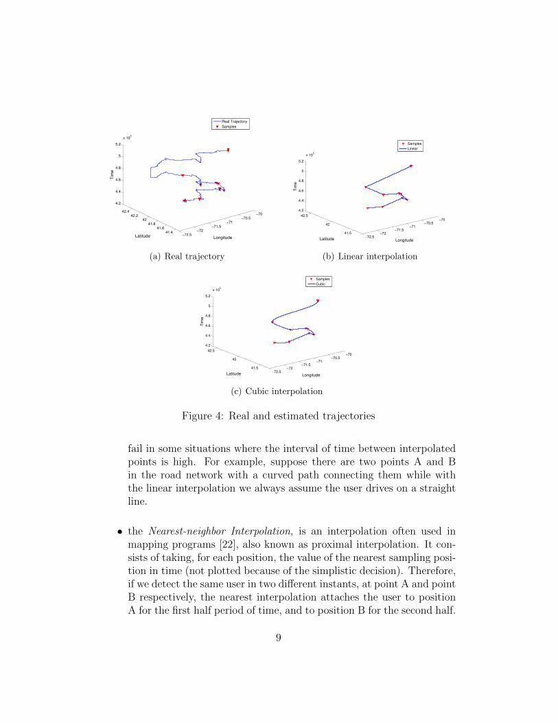
Different interpolation methods have been proposed in the literature todescribe moving object trajectories. We present in the following a selectionof classical ones, showing how they approximate the real trajectory (see anexample in Fig. 4).

• the Linear Interpolation, is a popular interpolation used in movementobjects databases [21]. It is presented in Fig. 4(b). It is obtainedby joining straight interpolating lines between each pair of consecutivesamples. Users are supposed to move at a constant speed along thestraight lines. One limitation of the linear interpolation is that it can

7The absolute length is of course overestimated with respect to the real one. Afterlooking into details, we discover that this is due to handover flipping among close antennas.The important aspect here remains the relative (and not the absolute) increasing trend.

8

−72.5−72

−71.5−71

−70.5−70

41.441.6

41.842

42.242.4

4.2

4.4

4.6

4.8

5

5.2

x 105

LongitudeLatitude

Tim

e

Real Trajectory

Samples

(a) Real trajectory

−72.5−72

−71.5−71

−70.5−70

41.5

42

42.5

4.2

4.4

4.6

4.8

5

5.2

x 105

LongitudeLatitude

Tim

e

Samples

Linear

(b) Linear interpolation

−72.5−72

−71.5−71

−70.5−70

41.5

42

42.5

4.2

4.4

4.6

4.8

5

5.2

x 105

LongitudeLatitude

Tim

e

Samples

Cubic

(c) Cubic interpolation

Figure 4: Real and estimated trajectories

fail in some situations where the interval of time between interpolatedpoints is high. For example, suppose there are two points A and Bin the road network with a curved path connecting them while withthe linear interpolation we always assume the user drives on a straightline.

• the Nearest-neighbor Interpolation, is an interpolation often used inmapping programs [22], also known as proximal interpolation. It con-sists of taking, for each position, the value of the nearest sampling posi-tion in time (not plotted because of the simplistic decision). Therefore,if we detect the same user in two different instants, at point A and pointB respectively, the nearest interpolation attaches the user to positionA for the first half period of time, and to position B for the second half.

9

• the Piecewise Cubic Hermite Interpolation is often used in image pro-cessing studies (see [23]). It is depicted in Fig. 4(c). It is a third-degreespline that interpolates the function by a cubic polynomial using valuesof the function and its derivatives at the ends of each subinterval. Thismethod interpolates the samples in such a way that the first derivativeis continuous, but the second derivative is not necessary continuous.The slopes are chosen in a way that the function is “shape preserv-ing” and respects monotonicity. Suppose a subinterval [x1, x2], withthe function values: y1 = f(x1), y2 = f(x2) and the derivative valuesd1 = f ′(x1) and d2 = f ′(x2) are given. The cubic polynomial functionin this subinterval is given by:

C(x) = a + b(x− x1) + c(x− x1)2 + d(x− x1)

2(x− x2) (2)

satisfying C(x1) = y1, C(x2) = y2, C′(x1) = d1 and C ′(x2) = d2 This

interpolation determines the coefficients a, b, c and d noting that:

C ′(x) = b + 2c(x− x1) + d[(x− x1)2 + 2(x− x1)(x− x2)] (3)

is also continuous. The solution to this system is given by: a = y1;

b = d1; c =y′1−d1x2−x1

and d =d1+d2−2y′1(x2−x1)2

, where y′1 = y2−y1x2−x1

.

4. Results

In this section, we present the main results obtained by applying theinterpolation methods introduced in Section 3.

First, we quantify the error, given by the ratio of the overall position de-viation (computed as described in Section 2.1) to the radius of gyration, forthe different interpolation methods. Then, we further investigate the statis-tical distribution of the errors with respect to mobility parameters in orderto understand what method performs better for each particular category ofusers.

4.1. Interpolation Error

Fig. 5 reports boxplot8 and average (the star) statistics about the inter-polation error (trajectory deviation to the radius of gyration), for the linear,

8i.e., first quartile, median, third quartile, maximum, minimum and outliers. It is worthnoting that some maximum and outliers are cut in the figure for the sake of readability.

10

nearest and cubic interpolations. Boxplot statistics give a compact and richenough view on the data to support the following analysis.

At a first view, looking at the error averages, we can assess that:

• The error is decreasing with the increase of the subsampling ratio,for whatever interpolation, which is reasonable as one can get moreaccurate computations with more samples.

• The gap between the three interpolation methods decreases with theincrease of the radius of gyration, especially for those users with a radiusof gyration higher than 10 km, i.e., those who could be considered asperi-urban users and commuters (see Section 2.2).

• The lowest mean error among different interpolation methods dependson the category to which the user belongs. Indeed, for those users hav-ing a radius of gyration less than 3 km, i.e., sedentary users, the linearinterpolation method presents the smallest mean error when comparedto other methods. Instead, for those users having a higher radius of gy-ration, especially for commuters (i.e., those with a radius of gyration ofmore than 32 km), the cubic interpolation presents the smallest meanerror. Finally, for urban users with a radius of gyration between 3 and10 km, the linear and cubic interpolations show close performance.

Therefore, we can confirm that the trajectory deviation strongly dependson the mobility category, i.e., the user radius of gyration. In order to de-termine the correlation function between the deviation and the radius ofgyration, Fig. 6 shows for each user (one point), given by its radius of gy-ration, the trajectory deviation (just for the linear interpolation, knowingthat other interpolation methods give a very similar trend). The trend beinggenerally increasing, we have positive correlation. Indeed, with the increaseof the radius of gyration, users are able to move over longer distances, thedistance between two samples increases, hence finding a good interpolationmethod that accurately approximates the real trajectory traversed by theuser gets more challenging.

Finally, further looking into the whole statistics of the errors, includingmedian and quartile lines, we can determine that:

• The median is always lower than the average, which indicates that thepopulation contains an important part of users with much higher errorsthan the rest of the population.

11

(a) rg<=3km (Sedentary Users) (b) 3km<rg<=10km (Urban Users)

(c) 10km<rg<=32km (Peri-urban Users) (d) rg>32km (Commuters)

Figure 5: Boxplots of the deviation to the radius of gyration error forclassical interpolation methods.

• Overall, the nearest interpolation shows better median statistics thanall the other interpolations for all user categories with different radiusof gyration.

• The median error becomes very low for subsampling ratio of more than0.1 for peri-urban and commuter users.

4.2. Interpolations’ Probability Density Function

How to explain the huge gap between averages and medians, and theperformance inversion indicating that nearest interpolation is on median the

12

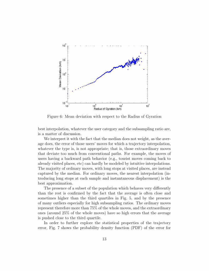
Figure 6: Mean deviation with respect to the Radius of Gyration

best interpolation, whatever the user category and the subsampling ratio are,is a matter of discussion.

We interpret it with the fact that the median does not weight, as the aver-age does, the error of those users’ moves for which a trajectory interpolation,whatever the type is, is not appropriate; that is, those extraordinary movesthat deviate too much from conventional paths. For example, the moves ofusers having a backward path behavior (e.g., tourist moves coming back toalready visited places, etc) can hardly be modeled by intuitive interpolations.The majority of ordinary moves, with long stops at visited places, are insteadcaptured by the median. For ordinary moves, the nearest interpolation (in-troducing long stops at each sample and instantaneous displacement) is thebest approximation.

The presence of a subset of the population which behaves very differentlythan the rest is confirmed by the fact that the average is often close andsometimes higher than the third quartiles in Fig. 5, and by the presenceof many outliers especially for high subsampling ratios. The ordinary movesrepresent therefore more than 75% of the whole moves, and the extraordinaryones (around 25% of the whole moves) have so high errors that the averageis pushed close to the third quartile.

In order to further explore the statistical properties of the trajectoryerror, Fig. 7 shows the probability density function (PDF) of the error for

13

(a) linear (b) nearest

(c) cubic

Figure 7: Probability density function of error - (subsampling ratio: 0-0.05)

the linear, cubic and nearest interpolations.It is easy to notice that there are two regimes. The distribution of errors

over all users’ positions is well approximated by a combination of two powerlaw distributions joined by a breakpoint. It is surprising to notice that thebreakpoint is the same (approximately equal to 2.2) for the different inter-polation methods. In practice, what does this power law breakpoint reallymean? We interpret it as the point after which the interpolation error prop-erties change abruptly. The value, around 2, corresponds to two times theuser’s radius of gyration, which in practice represents the user’s “territory”(the circle of radius equal to the radius of gyration). This is a meaningfulresult: trajectory interpolations are more appropriate within the territory of

14

Figure 8: Joint Probability of the Deviation to the radius of gyration Errorwith the normalized distance to the centroid

a user than outside it.In order to further evaluate this dependency, we normalize the user po-

sition by the corresponding radius of gyration, and we plot in Fig. 8 thejoint PDF of the normalized distance of users’ positions to the centroid ofthe trajectory with the trajectory error. The figure shows that when thesmallest errors occur, it is highly probable that the user is within the radiusof gyration (when the normalized distance to the centroid is less than 1), i.e.,the user’s territory; when the highest errors occur, it is highly probable thatthe user is outside the territory.

These values can alternatively be analyzed by the conditional cumulativedensity distribution of the two variables, error and the normalized distanceto centroid, as presented in Fig. 9. We can determine therein that:

• when small errors occur, we have a high probability (80.78%) that theuser is inside the territory, and a low probability (19.22%) the user isoutside it.

• When big errors occur, we have a probability of 40.25% that the user isinside its radius of gyration and a probability of 59.75% that the useris outside its radius.

Therefore, we have an additional experimental proof that the trajectory errorincreases and its characteristics change when the user moves beyond theterritory area roughly approximated by the radius of gyration.

15

(a) Distributions of the normalized distanceto the centroid when the deviation is lessthan 2.2 the radius of gyration

(b) Distributions of the normalized distanceto the centroid when the deviation is morethan 2.2 the radius of gyration

Figure 9: Conditional cumulative density function

5. Estimation of Hotspot Positions

A fundamental issue to be taken into account for the management ofbroadband mobile cellular networks is finding the best location for the de-ployment of adaptive content and cloud distribution solutions at the basestation and backhauling network level. Intuitively, an adaptive placementof content and computing resources in the most crowded regions can grantimportant traffic offloading, improve network efficiency and user quality ofexperience. We use thereafter the term “hotspots” to denote these regions. Alimited amount of work exists in the literature for the estimation of hotspotsand rendez-vous points in wireless access networks. E.g., in [24] vehiculardata is exploited to determine accident-risk points. Many other works, suchas [25], [26], [27] and [12], while assuming the availability of mobility in-formation, focus in user-profile aware QoS provisioning, load balancing andnetwork signaling improving techniques.

Traffic load forecasting has also been investigated from an analytical andmathematical modeling perspective. For example, authors in [28] show howunder certain conditions periodic sinusoidal functions can be used as cellu-lar traffic profile. Unfortunately the simplicity and the too theoretical ap-proaches fail from precisely matching with the actual real traffic load, whichis a strict requirement of our investigation.

Motivated by the usage of signaling mobile phone data that give real tra-

16

Figure 10: Real Block Load

jectories of smartphone users, we extract in this section real hotspot positionsand compare them with the estimated positions that one can get by applyingthe interpolation methods defined above.

Decomposing the state of Massachusetts into census blocks9[29] , we com-pute the real load of each block in the region (i.e., expressed as the users’number of visits to each block) as shown in Fig. 10.

The small map in the upper right corner is a zoom in of the Boston urbanarea, the state’s largest city where small blocks exist. The figure clearly showsthe load difference among the blocks and the existence of crowded blocks thatdefine the most visited places where large masses of people usually visit.

Then, we estimate the load of each of these blocks by choosing for eachuser category the best interpolation method obtained in the results before(i.e. for sedentary and urban mobile users, we use the linear interpolationmethod to join the samples, while for peri-urban mobile users and the com-muters we follow the cubic interpolation).

9A census block is the smallest geographic unit used by the United States CensusBureau. Blocks are typically bounded by streets, roads or creeks.

17

Figure 11: Estimated Block Load

After these, we compute the estimated block load. The results are ob-tained in Fig. 11, one can notice that the load is overestimated especiallyfor the less crowded blocks. But what about the hotspots? How does theestimation error vary for the most crowded places?

Fig. 12 represents the variation of the estimation error with respect to thereal load. In-line with ones exceptional for a statistically good estimation,we can state that:

• The estimation error is very high for the less visited blocks in the region.

• The estimation error rapidly decreases with the increase of the realload.

• For the most crowded blocks, we notice that the estimation error issignificantly smaller.

By choosing different thresholds beyond which we identify the hotspotblocks (i.e., if a block has a load, expressed by the total number of users’visits during the day, that exceeds the chosen threshold it is considered asa hotspot block.), we plot for each case the cumulative distribution function

18

101

102

103

104

105

10−4

10−3

10−2

10−1

100

101

Real Load

Lo

ad

Estim

atio

n E

rro

r

All users

Figure 12: Load Estimation Error

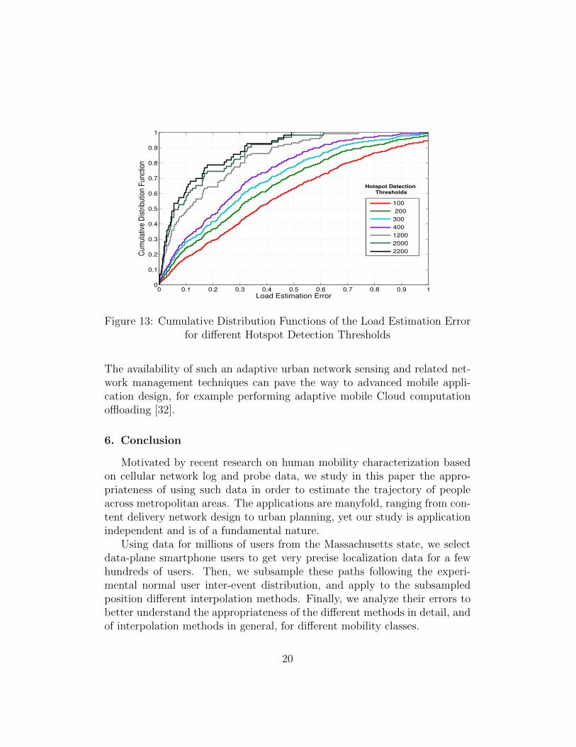
of the block load estimation error. The results are shown in Fig. 13. We canstate that:

• The median estimation error decreases with the increase of the realblock load.

• The median estimation error reaches 7% for blocks of more than 2000visits per day while for those with more than 100 visits per day, we getan error of 36%.

As a conclusion we can clearly confirm that the interpolation methods wehave evaluated in this paper are able to find the hotspot positions with a smallmedian error. We should note here that the proposed hotspot estimationmethod is scalable in a way that, taking a sample of users instead of thewhole population enables us to find the hotspot positions in a relativelyaccurate way.

The online estimation of hotspot positions we propose is therefore veryaccurate and shows interesting properties in support of advanced urban com-puting services. A context of application could be that of content offload-ing [30] or Cloud offloading in mobile access networks: detecting hotspotpositions in the backhauling network can allow adaptively allocating contentcaches or dimensioning CloudLet resources [31] for location-sensitive services.

19

0 0.1 0.2 0.3 0.4 0.5 0.6 0.7 0.8 0.9 10

0.1

0.2

0.3

0.4

0.5

0.6

0.7

0.8

0.9

1

Load Estimation Error

Cu

mu

lative

Dis

trib

utio

n F

un

ctio

n

100

200

300

400

1200

2000

2200

Hotspot Detection Thresholds

Figure 13: Cumulative Distribution Functions of the Load Estimation Errorfor different Hotspot Detection Thresholds

The availability of such an adaptive urban network sensing and related net-work management techniques can pave the way to advanced mobile appli-cation design, for example performing adaptive mobile Cloud computationoffloading [32].

6. Conclusion

Motivated by recent research on human mobility characterization basedon cellular network log and probe data, we study in this paper the appro-priateness of using such data in order to estimate the trajectory of peopleacross metropolitan areas. The applications are manyfold, ranging from con-tent delivery network design to urban planning, yet our study is applicationindependent and is of a fundamental nature.

Using data for millions of users from the Massachusetts state, we selectdata-plane smartphone users to get very precise localization data for a fewhundreds of users. Then, we subsample these paths following the experi-mental normal user inter-event distribution, and apply to the subsampledposition different interpolation methods. Finally, we analyze their errors tobetter understand the appropriateness of the different methods in detail, andof interpolation methods in general, for different mobility classes.

20

The major findings of our work can be summarized as follows.

• The radius of gyration is an appropriate, compact and easy to com-pute parameter to qualify user mobility in a metropolitan area networkscope.

• The linear interpolation is the best approximation for sedentary users,linear and cubic interpolations work well for urban users, and the cubicinterpolation is the best for peri-urban users and commuters.

• Separating ordinary moves following conventional paths from the mi-nority of user moves with unpredictable displacements, the nearest in-terpolation is by far the best approach whatever the mobility class is.

• Interpolation methods clearly work better when applied within the ter-ritory of the user defined by the radius of gyration.

• Interpolation methods are able to find the hotspot positions of the mostcrowded places with a very high precision.

As already mentioned, we believe the applications are manyfold. We arein particular interested in determining how content and Cloud delivery pointsin an urban and peri-urban environments can be identified and adapted onlineby inferring basic user mobility properties from big data log coming fromcellular networks.

Acknowledgment

The authors would like to thank Airsage for providing the data used forthe experiments.

We further thank Ericsson, the MIT SMART Program, the Center forComplex Engineering Systems (CCES) at KACST and MIT CCES program,the National Science Foundation, the MIT Portugal Program, the AT&TFoundation, Audi Volkswagen, BBVA, The Coca Cola Company, Expo 2015,Ferrovial, The Regional Municipality of Wood Buffalo and all the membersof the MIT Senseable City Lab Consortium for supporting the research.

This work was partially supported by the ANR ABCD project (GrantNo: ANR-13-INFR-005), and by the EU FP7 IRSES MobileCloud Project(Grant No. 612212).

21

[1] S. Hoteit, S . Secci, S. Sobolevsky, G. Pujolle and C. Ratti “Estimat-ing Human Trajectories through Mobile Phone Data”, in Proc. of 2013IEEE Int. Conference on Mobile Data Management (IEEE MDM 2013),Human Mobility Computing Workshop, 3-6 June, 2013, Milan, Italy.

[2] M. Gonzalez, CA . Hidalgo, Al. Barabasi “Understanding individualhuman mobility patterns”, Nature 458, pp. 238-238, 2008.

[3] H. Hohwald, E. Frias-Martinez, and N. Oliver “User modeling fortelecommunication applications: Experiences and practical implications”,in Proc. UMAP, pp. 327-338, 2010.

[4] R. Huerta, L. Tsimring “Contact tracing and epidemics control in socialnetworks”, Physical Review E 66, 2002.

[5] P. Wang, MC. Gonzalez, CA . Hidalgo, Al. Barabasi “Understanding thespreading patterns of mobile phone viruses”, Science 324, pp. 1071-1076,2009.

[6] F. Calabrese, F. Pereira, G. Di Lorenzo, L. Liu, C. Ratti “The Ge-ography of Taste: Analyzing Cell-Phone Mobility and Social Events”,In Proc. of 2010 IEEE Int. Conf. on Pervasive Computing (PerComp),2010.

[7] M. Turner, S. Love, M. Howell, “Understanding emotions experiencedwhen using a mobile phone in public: The social usability of mobile(cellular) telephones”, Telemat. Inf. 25:3, pp. 201-215, 2008.

[8] R.C. Nickerson, H. Isaac, B. Mak “A multi-national study of attitudesabout mobile phone use in social settings”, Int. J. Mob. Commun. 6:5,541-563, 2008.

[9] S. Hoteit, S. Secci, Z. He, C. Ziemlicki, Z. Smoreda, C. Ratti, G. Pujolle“Content Consumption Cartography of the Paris Urban Region usingCellular Probe Data”, in Proc. of ACM URBANE 2012, CoNext 2012Workshop, 2012.

[10] M. R. Vieira, V. Frias-Martinez, N. Oliver and E. Frias-Martinez, “Char-acterizing dense urban areas from mobile phonecall data: Discovery andsocial dynamics”, in Proc. IEEE SocialCom, pp. 241-248, 2010.

22

[11] H. Wang, F. Calabrese, G. Di Lorenzo and C. Ratti, “Transportationmode inference from anonymized and aggregated mobile phone call detailrecords”, Proc. IEEE ITSC, pp. 318-323, 2010.

[12] H. Zang, J. Bolot, “Mining call and mobility data to improve pagingefficiency in cellular networks”, in Proc. of 2007 ACM Int. Conf. onMobile Computing and Networking (ACM MOBICOM 2007).

[13] L. Wei, Y. Zheng, W. Peng “Constructing Popular Routes from Un-certain Trajectories”, 18th SIGKDD conference on Knowledge Discoveryand Data Mining, KDD 2012.

[14] K. Zheng, Y. Zheng, X. Xie, and X. Zhou “Reducing Uncertainty ofLowSampling-Rate trajectories”, In IEEE International Conference onData Engineering, ICDE, 2012.

[15] T. Hagerstrand, “What about people in regional science?”, Papers inRegional Science 24:1, pp. 6-21, December 1970.

[16] S. Winter and Z.C. Yin, “Directed movements in probabilistic timegeography”, International Journal of Geographical Information Science24, pp. 1349-1365, 2010.

[17] M. Ficek and L. Kencl, “Inter-Call Mobility Model: A Spatio-temporalRefinement of Call Data Records Using a Gaussian Mixture Model”, InProc. of IEEE INFOCOM, 2012

[18] I.Rhee, M.Shin, S.Hong, K.Lee, S.J.Kim, S.Chong, “On the levy-walknature of human mobility”, in Proc. of INFOCOM 2008.

[19] Airsage: Airsage WISE technology, http://www.airsage.com.

[20] C. Schneider, T. Couronne, Z. Smoreda, M. Gonzalez, “Are we in ourtravel decisions self-determined?”, Bulletin of the American Physical So-ciety, APS, 2012.

[21] R. H. Guting and M. Schneider, Moving Objects Databases, MorganKaufmann, 2005.

[22] C. S. Yang, S. P. Kao, F. B. Lee and P . S . Hung, “Twelve differentinterpolation methods: A case study of Surfer 8.0”, in Proc. of XXthISPRS, 2004.

23

[23] F.N. Fritsch and R. E Carlson, “Monotone piecewise cubic interpola-tion”, SIAM Journal of Numerical Analysis 17, 238-246, 1980.

[24] TK. Anderson “Kernel density estimation and K-means clustering toprofile road accident hotspots”, Accident Analysis and Prevention, Vol.41, No. 3, 2009.

[25] K. Seada “Rendezvous regions: a scalable architecture for service loca-tion and data-centric storage in large-scale wireless networks”, in Proc.of 2004 Parallel and Distributed Processing Symposium.

[26] S.K. Das, S.K.S. Jayaram “A novel load balancing scheme for the tele-traffic hot spot problem in cellular networks”, Wireless Networks, Vol. 4,No. 4, 2004.

[27] D. Ghosal, B. Mukherjee“Exploiting user profiles to support differenti-ated services in next-generation wireless networks”, IEEE Networks, Vol.18, No. 5, 2004.

[28] E. Oh and B. Krishnamachari, “Energy Savings through Dynamic BaseStation Switching in Cellular Wireless Access Networks”, In Proc. ofIEEE Globecom 2010.

[29] US census Bureau, http://www2.census.gov/

[30] V. Jacobson, D.K. Smetters, J.D. Thornton, M. Plass, N. Briggs andR. Braynard “Networking Named Content”, CoNEXT ’09 .

[31] M. Satyanarayanan, P. Bahl, R. Caceres and N. Davies “The Case forVM-based Cloudlets in Mobile Computing”, IEEEPervasive Computing,8(4), 2009..

[32] L. Jiao, R. Friedman, X. Fu, S. Secci, Z. Smoreda and Hannes Tschofenig“Challenges and Opportunities for Cloud-based Computation Offloadingfor Mobile Devices”, in Proc. of Future Network and Mobile Summit,2013.

24