estimating macroeconomic models of financial crises: an
TRANSCRIPT
Estimating Macroeconomic Models of Financial Crises:An Endogenous Regime Switching Approach∗
Gianluca BenignoLondon School of Economics
CEPR
Andrew FoersterFederal Reserve Bank of Kansas City
Christopher OtrokUniversity of Missouri
Federal Reserve Bank of St. Louis
Alessandro RebucciJohns Hopkins University
NBER
February 28, 2018
Abstract
We develop a novel approach to specifying, solving and estimating Dynamic Struc-tural General Equilibrium (DSGE) models of financial crises. We first propose anew specification of the standard Kiyotaki-Moore type collateral constraint wherethe movement from the unconstrained state of the world to constrained state is astochastic function of the endogenous leverage ratio in the model. This specificationresults in an endogenous regime switching model. Next, we develop perturbationmethods to solve this model. Using the second order solution of the model, we thendesign an algorithm to estimate the parameters of the model with full-informationBayesian methods. Applying the framework to quarterly Mexican data since 1981,we find that the model’s estimated crisis regime probabilities correspond closely withnarrative dates for Sudden Stops in Mexico. Our results also shows that fluctuationsin the non-crisis regime of the model are driven primarily by real shocks, while lever-age shocks are the prime driver of the crisis regime. The paper provides the firstset of structural estimates of financial shocks stressed in the normative literature andconsistent with available reduced form evidence finding that financial/credit shocksonly matter in crisis periods.
Keywords: Financial Crises, Regime Switching, Bayesian Estimation, Leverage Shocks.JEL Codes: G01, E3, F41, C11.
∗Corresponding author: Christopher Otrok: [email protected], phone 434-227-1928, address: 909University Avenue, 118 Professional Building, Columbia, MO 65211-6040. Other email addresses, Gian-luca Benigno: [email protected]. Andrew Foerster: [email protected]. Alessandro Rebucci:[email protected]
1

Solving and Estimating Models of Financial Crises:An Endogenous Regime Switching Approach
Gianluca Benigno1 Andrew Foerster2
Christopher Otrok3 Alessandro Rebucci4
1London School of Economics and CEPR
2Federal Reserve Bank of Kansas City
3University of MissouriFederal Reserve Bank of St Louis
4Johns Hopkins University and NBER
BFOR Endogenous Switching 1 / 44

Introduction
Motivation
Global financial crisis proved very costly to resolve
Long history of painful financial crises in emerging markets
A large theoretical literature has emerged in responseI Models of collateral constraints for amplification of shocksI Normative analyses of inefficiencies associated with collateral
constraintsI Debate over ex-ante versus ex-post policiesI Debate over which instruments are most effective
BFOR Endogenous Switching 2 / 44

Introduction
Missing piece in financial crisis literature
Quantitative analysis of financial crises in estimated models withoccasionally binding constraints
I Which shocks drive crises? Are they the same that drive normal cycles?I Is there time variation in the importance of those shocks?I How do the dynamic responses to shocks change when collateral
constraints bind?
One can then return to the theoretical questions of when shouldpolicy makers intervene and with which instruments?
I Does it matter what shocks drive crises?I Which instruments best address which shocks?
BFOR Endogenous Switching 3 / 44

Introduction
Pre-Crisis and Post-Crisis Consensus on Methodology
Pre-crisis: Medium scale estimated linear DSGE modelsI Estimate importance of shocks and frictionsI Analyze policy questions in this fully specified empirical frameworkI Non-linearity restricted to 2nd order solution of model
Post-Crisis: Events studies with calibrated models featuring non-lineardynamics
I Non-linearity often in the form of occasionally binding borrowingconstraints
This paper bridges the two approaches by providing an empiricalframework that allows for estimation of shocks and frictions while atthe same time incorporating the nonlinearities associated withfinancial crises
BFOR Endogenous Switching 4 / 44

Introduction
Overview
New approach to specifying, solving and estimating models offinancial crises
I Financial crises are rare but large events → model must be non-linearI Non-linearity poses computational problemsI We provide a tractable formulation of collateral constraint and then
develop methods to solve and estimate a model with such a constraint
We set up a model with a Kiyotaki-Moore type of collateral constraint
I The constraint limits total debt to a fraction of the market value ofphysical capital (it is a limit on leverage)
I Constraint imposed on the agents as in Kiyotaki and Moore (1997),Aiyagari and Gertler (1999), Kocherlakota (2000) and Mendoza (2010)
I Constraint is not derived from an optimal contract, but is motivated bythe optimal contracting literature
BFOR Endogenous Switching 5 / 44

Introduction
Overview (Cont.)
We propose a new specification of such a collateral constraintI We model the movement from unconstrained state of the world to
constrained state as a stochastic function of the LTV ratio (or leverageratio)
F We can then write constraint as a regime switching processF One regime in which the constraint binds (a crisis regime)F One regime in which it does not bind (normal regime)
I Probability of the collateral constraint binding rises with leverageF This captures the fact that the likelihood of a crisis raises with
leverage, without requiring a crisis to occurF Agents in the model know that higher leverage levels (and lower
collateral values) increase the probability of a financial crisis
Our constraint specification is an endogenous regime switching model
BFOR Endogenous Switching 6 / 44

Introduction
Overview–cont.
We develop a solution method for endogenous regime switchingmodels
I The solution is an approximation around a steady state which is theaverage of the deterministic steady state in the two regimes, weightingwith ergodic probabilities
Some features of our solution methodI We solve with perturbation methods: we can handle multiple state
variables and many shocksI Second order approximation: Capture impact of risk on decision rulesI Fast solution method → non-linear filters can be used to calculate the
likelihood functionI Structural model would allow us to perform policy counterfactuals
(future work)
BFOR Endogenous Switching 7 / 44

Introduction Outline
Outline of Talk
Model
Collateral Constraint Formulation
Solution
Properties of Model Solution
Estimation Procedure
Empirical Results
BFOR Endogenous Switching 8 / 44

Model
Structure and Utility
Small open economyI Bianchi and Mendoza (2015) and Huo and Rios-Rull (2016) apply this
setup even to the United States
Model very similar to Mendoza (2010), but different specification ofthe borrowing constraint and set of shocks considered
Consumer Utility with GHH preferences
U ≡ E0
∞∑t=0
{βt
1
1− ρ
(Ct −
Hωt
ω
)1−ρ}
BFOR Endogenous Switching 9 / 44

Model
Production and Constraints
Production uses capital, labor and imported intermediate goods
Yt = AtKηt−1H
αt V
1−α−ηt
There is a working capital requirement
φrt (WtHt + PtVt)
Investment subject to adjustment costs
It = δKt−1 + (Kt − Kt−1)
(1 +
ι
2
(Kt − Kt−1
Kt−1
))Budget constraint
Ct + It = Yt − PtVt − φrt (WtHt + PtVt)−1
(1 + rt)Bt + Bt−1
Bt < 0 denotes the debt position at the end of period t
BFOR Endogenous Switching 10 / 44

Model Collateral Constraint
Collateral Constraint
The agent faces a regime specific collateral constraint
In regime 1 (the crisis regime) the constraint binds, and totalborrowing is equal to a fraction of the value of collateral:
1
(1 + rt)Bt − φ (1 + rt) (WtHt + PtVt) = −κtqtKt
I Both debt and and working capital are restrictedI Collateral in the model is defined over the value of capitalI The price and quantity of collateral are endogenous (since this relative
price is in the constraint, there is the pecuniary externality emphasizedin the normative literature)
BFOR Endogenous Switching 11 / 44

Model Collateral Constraint
Collateral Constraint
In regime 0 (the normal regime) the constraint is slack, and collateralvalue is sufficient for international lenders to finance all desiredborrowing
I There is no explicit constraint on borrowing in this regimeI A small debt elastic interest rate premium prevents infinite debt
Define a new variable (the ”borrowing cushion”) which measures thedistance between debt and the value of collateral that constraintsborrowing
B∗t =1
(1 + rt)Bt − φ (1 + rt) (WtHt + PtVt) + κtqtKt
When the borrowing cushion is small the leverage ratio is high
BFOR Endogenous Switching 12 / 44

Model Collateral Constraint
Collateral Constraint
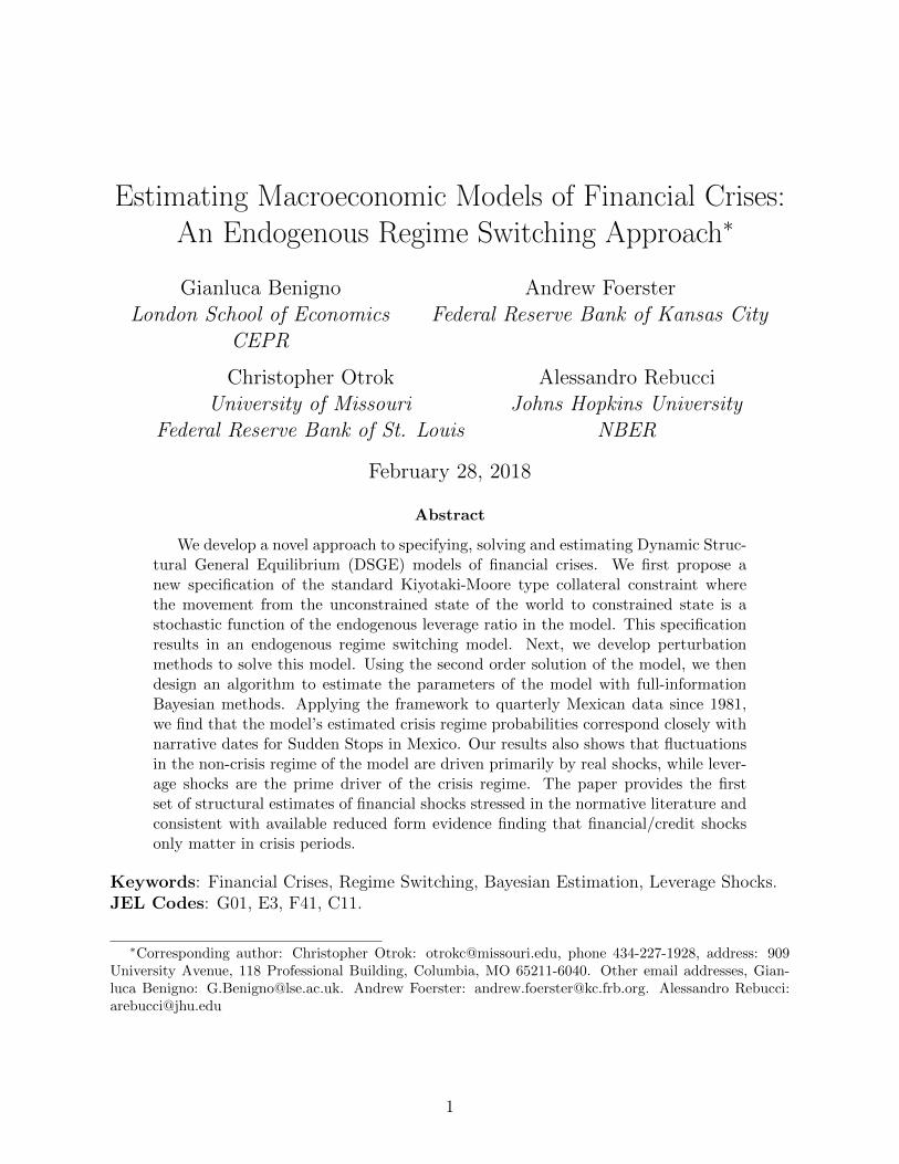
In regime 0 (non-binding) the probability that constraint binds thenext period depends the borrowing cushion
Pr (st+1 = 1|st = 0) =exp (γ0,0 − γ0,1B∗t )
1 + exp (γ0,0 − γ0,1B∗t )
The logistic function reformulates the Kiyotaki-Moore idea thatincreased leverage leads to binding collateral constraints as aprobabilistic statement
The transition probability from regime 0 to regime 1 is a function ofall endogenous variables in B∗t
BFOR Endogenous Switching 13 / 44
Model Collateral Constraint
As parameter γ0 gets large we recover the deterministic step function of the
literature as a special case
−0.1 −0.08 −0.06 −0.04 −0.02 0 0.02 0.04 0.06 0.08 0.10
0.2
0.4
0.6
0.8
1
B*t
Prob(st+1
=0|st=0,B*
t)
γ = 1000γ = 100
−0.1 −0.08 −0.06 −0.04 −0.02 0 0.02 0.04 0.06 0.08 0.10
0.2
0.4
0.6
0.8
1
Prob(st+1
=1|st=1,λ
t)
λt
BFOR Endogenous Switching 14 / 44

Model Collateral Constraint
Empirical motivation for our formulation
Borrowing constraints don’t bind at any particular LTV ratio in thereal world, they are are stochastic functions of LTV ratios
When a borrower hits the LTV limit, expenditure is adjusted graduallybecause other source of financing such as cash, precautionary creditlines, asset sales, etc. can be tapped into
I Capello, Graham, and Harvey (JFE, 2010) survey information onbehavior of financially constrained firms
I Ivashina and Scharfstein (JFE, 2010) loan level data show creditorigination dropped during the crisis because firms drew down frompre-existing credit lines in order to satisfy their liquidity
BFOR Endogenous Switching 15 / 44

Model Collateral Constraint
Collateral Constraint
Our model has the usual slackness condition B∗t λt = 0
In the binding Regime 1 the Lagrange multiplier λt , associated withthe constraint is strictly positive. The transition probability to goback to regime 0 is given by
Pr (st+1 = 0|st = 1) =exp (γ1,0 − γ1,1λt)
1 + exp (γ1,0 − γ1,1λt)
As the multiplier approaches 0, the probability of transitioning backto the non-binding state rises
Prior on γ1,0 can impose that probability of negative multiplier is verysmall
BFOR Endogenous Switching 16 / 44

Model Shocks
Shocks
There are 5 shocks (2 real, 3 financial): productivity, terms of trade,and leverage, risk premium, world interest rate,
Interest rate process has endogenous and exogenous components
rt = (ψr + σrεr ,t)(eB−Bt − 1
)+ (r∗ + σwεw ,t)
The TFP and TOT processes:
logAt = (1− ρA(st))a (st) + ρA (st) logAt−1 + σA (st) εA,t
logPt = (1− ρP(st))p (st) + ρP (st) logPt−1 + σP (st) εP,t
I The means and persistence of these shocks are regime dependent
BFOR Endogenous Switching 17 / 44
Model Shocks
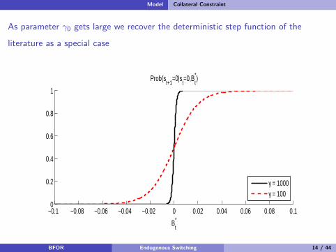
Leverage Shocks
Restrictions on leverage are stochastic, and may depend on regime
Binding regime
1
(1 + rt)Bt − φ (1 + rt) (WtHt + PtVt) = −κtqtKt
Nonbinding regime
B∗t =1
(1 + rt)Bt − φ (1 + rt) (WtHt + PtVt) + κtqtKt
Where
κt = (1− ρκ(st))κ (st) + ρκ (st)κt−1 + σκ (st) εκ,t
BFOR Endogenous Switching 18 / 44

Solution
Solution
The FOCs, constraints and shocks yield 16 equilibrium conditionsI This is the full set of structural equations of the model
The model as written is a nonlinear model similar to the literatureand can in principle be solved with global solution methods
We compute an approximate solution by solving the model around asteady state
I This steady state is an average of the steady states associated with thetwo regimes weighting with ergodic probabilities
I The perturbation solution includes a term that corrects for the fact thatthe switching model is either above or below this approximation point
BFOR Endogenous Switching 19 / 44

Solution
Markov Switching DSGE Literature
Large literature on Markov-switching linear rational expectationsmodels (MSLREs) with exogenous switching
I Leeper and Zha (2003), Davig and Leeper (2007), Farmer, Waggoner,and Zha (2009)
Foerster et al (2016) developed a perturbation method forconstructing first and second order solution of exogenousMarkov-switching DSGE models (MSDSGE)
I A key innovation in their paper is to work with the original MSDSGEmodel directly
Small literature on endogenous switching DSGE modelsI Davig and Leeper (2006), Lind (2014) Barthelemy and Marx (2016)
BFOR Endogenous Switching 20 / 44

Solution Regime Switching
Regime Switching: Approximation
We introduce two indicator variables that allow the regime switchingto affect both the slope and intercept of the decision rules:
I The variables ϕ (st) = γ (st) = st turn ”on” and ”off” the collateralconstraint, depending on the regime
The borrowing constraint for the two regimes can then be written:
ϕ (st)B∗ss+γ (st) (B∗t − B∗ss) = (1− ϕ (st))λss+(1− γ (st)) (λt − λss)
Where SS denotes a steady stateWith this function:
I When st = 0, then ϕ (0) = γ (0) = 0 and the equation simplifies to
λt = 0
I When st = 1, then ϕ (1) = γ (1) = 1 and the equation simplifies to
B∗t = 0
BFOR Endogenous Switching 21 / 44

Solution Regime Switching
Regime Switching: Approximation
Approximate constraint again:
ϕ (st)B∗ss+γ (st) (B∗t − B∗ss) = (1− ϕ (st))λss+(1− γ (st)) (λt − λss)
This equation also pins down the correct steady state valuesI Following FRWZ (2014) only the switching variable ϕ (st) is perturbedI The steady state slackness condition then satisfies
ϕ̄B∗ss = (1− ϕ̄)λss
I ϕ̄ is the ergodic mean of ϕ (st)I If only the non-binding regime occurs, then ϕ̄ = 0 and
λss = 0
I If only the binding regime occurs then ϕ̄ = 1 and
B∗ss = 0
BFOR Endogenous Switching 22 / 44

Solution Equilibrium
Regime Switching: Equilibrium
Recall that the model has 16 equilibrium conditions, in vector form:
Et f (yt+1, yt , xt , xt−1, χεt+1, εt , θt+1, θt) = 0
where θt is the vector of model parameters and the subset for thestochastic processes is regime dependent (θS ,t)
Predetermined variables:
xt−1 = [Kt−1,Bt−1, κt−1,At−1,Pt−1]
Non-predetermined variables:
yt = [Ct ,Ht ,Vt , It , kt , rt , qt ,Wt , µt , λt ,B∗t ]
5 shocks:εt = [εA,t , εw ,t , εP,t , εκ,t , εr ,t ]
BFOR Endogenous Switching 23 / 44

Solution Perturbation
Regime Switching: Perturbation Solution
The perturbation solution takes the stacked equilibrium conditionsand differentiates with respect to (xt−1, εt , χ), producing acomplicated polynominal system
We solve this polynomial system by finding a fixed point of asequence of eigenvalue problems
This procedure finds a single solution, but does not guaranteeuniqueness
If desired second order system can also be solved
Second order solution is critical for endogenous switching model:I We show that the first order solution of the endogenous switching is
identical to the first order solution of an exogenous switching model,but the second order solution differs
I Interpretation: precautionary behavior in the second order solution iscritical for endogenous switching to matter
BFOR Endogenous Switching 24 / 44

Properties of Solution
Solution Results
IRF to shocks for different parameterizations of the model
We compute solution for endogenous switching, exogenous switchingand no switching
I Does endogenous switching matter?
IRF is computed assuming we stay in the state (binding or not)
BFOR Endogenous Switching 25 / 44
Properties of Solution
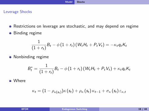
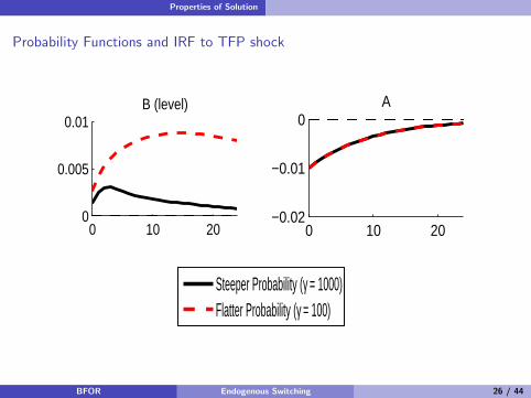
Probability Functions and IRF to TFP shock
0 10 20−0.01
−0.005
0K
0 10 200
0.005
0.01B (level)
0 10 20−2
0
2x 10
−17 P
0 10 20−0.02
−0.01
0A
0 10 20−0.02
−0.01
0C
0 10 20−0.01
−0.005
0H
0 10 20−0.02
−0.01
0V
0 10 20−0.1
−0.05
0I
0 10 20−0.01
−0.005
0k
0 10 20
−4
−2
0x 10
−4 r (pp)
0 10 20−5
0
5x 10
−3 Q
0 10 20−0.01
−0.005
0W
0 10 200
0.01
0.02µ
0 10 20−1
0
1λ (level)
0 10 20−0.02
−0.01
0B* (level)
0 10 20−0.02
−0.01
0Y
0 10 20−0.02
−0.01
0B/Y (level)
Steeper Probability (γ = 1000)Flatter Probability (γ = 100)
0 10 20−0.01
−0.005
0K
0 10 200
0.005
0.01B (level)
0 10 20−2
0
2x 10
−17 P
0 10 20−0.02
−0.01
0A
0 10 20−0.02
−0.01
0C
0 10 20−0.01
−0.005
0H
0 10 20−0.02
−0.01
0V
0 10 20−0.1
−0.05
0I
0 10 20−0.01
−0.005
0k
0 10 20
−4
−2
0x 10
−4 r (pp)
0 10 20−5
0
5x 10
−3 Q
0 10 20−0.01
−0.005
0W
0 10 200
0.01
0.02µ
0 10 20−1
0
1λ (level)
0 10 20−0.02
−0.01
0B* (level)
0 10 20−0.02
−0.01
0Y
0 10 20−0.02
−0.01
0B/Y (level)
Steeper Probability (γ = 1000)Flatter Probability (γ = 100)
BFOR Endogenous Switching 26 / 44

Properties of Solution
IRF in Non-binding state: large versus small crisis (TFP Shock)
0 10 20−0.01
−0.005
0K
0 10 20−0.05
0
0.05B (level)
0 10 20−5
0
5x 10
−17 P
0 10 20−0.02
−0.01
0A
0 10 20−0.02
−0.01
0C
0 10 20−0.01
−0.005
0H
0 10 20−0.02
−0.01
0V
0 10 20−0.1
−0.05
0I
0 10 20−0.01
−0.005
0k
0 10 20−2
0
2x 10
−3 r (pp)
0 10 20−5
0
5x 10
−3 Q
0 10 20−0.01
−0.005
0W
0 10 200
0.01
0.02µ
0 10 20−1
0
1λ (level)
0 10 20−0.04
−0.02
0B* (level)
0 10 20−0.02
−0.01
0Y
0 10 20−0.02
−0.01
0B/Y (level)
Smaller CrisisLarger Crisis
BFOR Endogenous Switching 27 / 44

Properties of Solution
IRF in Non-binding state: large versus small crisis (1st order solution, TFP Shock)
0 10 20−0.01
−0.005
0K
0 10 200
0.01
0.02B (level)
0 10 200
2
4x 10
−18 P
0 10 20−0.02
−0.01
0A
0 10 20−0.02
−0.01
0C
0 10 20−0.01
−0.005
0H
0 10 20−0.02
−0.01
0V
0 10 20−0.1
−0.05
0I
0 10 20−0.01
−0.005
0k
0 10 20−1
−0.5
0x 10
−3 r (pp)
0 10 20−5
0
5x 10
−3 Q
0 10 20−0.01
−0.005
0W
0 10 200
0.01
0.02µ
0 10 20−1
0
1λ (level)
0 10 20−4
−2
0x 10
−3 B* (level)
0 10 20−0.02
−0.01
0Y
0 10 20−0.02
0
0.02B/Y (level)
Smaller CrisisLarger Crisis
BFOR Endogenous Switching 28 / 44

Estimation
Bayesian Full Information Likelihood Methods for Nonlinear Models
We cannot assume that the parameters in one regime are independentof parameters of the other regime → two step procedures areinappropriate in our case (e.g. Aruoba, Cuba-Borda, Schorfheide(2014), Bocola (2016))
I Agents in the model fully understand that a crisis may occur, andadjust their behavior accordingly
I Our estimated model is useful for normative analysis precisely becauseof this feature of the model solution/estimation
We need a procedure for simultaneous estimation of regime switchand parameters in each regime
Second order solution neededI Bianchi (2014) estimates MSLRE with first order solution
BFOR Endogenous Switching 29 / 44

Estimation
Estimation: Bayesian Full Information Likelihood Methods
We use a Metropolis-in-Gibbs Sampling procedureI Conditional on regimes, draw parameters using the standard MH
algorithmF Given parameters, regimes, data, the value of the likelihood function is
computed with a Sigma Point FilterF The Sigma Point Filter is used in conjunction with the second order
solution of the modelF The value of the posterior is then computed after evaluating priors
I Conditional on parameters, data, draw regimes
BFOR Endogenous Switching 30 / 44

Estimation Results
Estimation from 1981.Q1 to 2016.Q1
Real GDP Growth, Investment growth, Consumption Growth, ImportPrice Growth
Interest rate: (EMBI Global + world interest rate (3month T-Bill rate- US expected inflation))
BFOR Endogenous Switching 31 / 44

Estimation Results
Basic Calibration
Table: Basic Calibration
Parameter Calibrated Value
Discount Factor β 0.97959Risk Aversion ρ 2Labor Share α 0.592
Capital Share η 0.306Wage Elasticity of Labor Supply ω 1.846
Capital Depreciation δ 0.022766
Debt to Output Ratio BY -0.86
Interest Rate Elasticity ψr 0.001Mean of TFP Process, Normal Regime a(0) 0
Mean of Import Price Process, Normal Regime p(0) 0Mean of Leverage Process, Normal Regime κ(0) 0.15
BFOR Endogenous Switching 32 / 44

Estimation Results
Prior and Posterior: Preliminary Estimation Results
Table: Some key structural parameters
Parameter Prior Posterior mean q5 q95γ0 Uniform(0,1000) 163.8018 162.0918 166.0587γ1 Uniform(0,1000) 111.8985 107.9163 114.5517ι Uniform(0,100) 2.6520 2.6490 2.6557φ Uniform(0,100) 0.2588 0.2572 0.2608
BFOR Endogenous Switching 33 / 44

Estimation Results
Posterior of Logistic Function
−0.1 −0.08 −0.06 −0.04 −0.02 0 0.02 0.04 0.06 0.08 0.10
0.1
0.2
0.3
0.4
0.5
0.6
0.7
0.8
0.9
1
Pr(st+1
=0|st=0,B*
t)
Figure: Transition prob. of nonbinding conditional on nonbinding
BFOR Endogenous Switching 34 / 44

Estimation Results
Prior and Posterior: Preliminary Estimation Results
Table: Shock Standard Deviations
Parameter Prior Posterior mean q5 q95σr (0) Uniform(0,1) 0.0023 0.0014 0.0031σr (1) Uniform(0,1) 0.0104 0.0098 0.0109σw (0) Uniform(0,1) 0.0017 0.0014 0.0019σw (1) Uniform(0,1) 0.0181 0.0175 0.0189σa(0) Uniform(0,1) 0.0065 0.0056 0.0075σa(1) Uniform(0,1) 0.0077 0.0069 0.0084σp(0) Uniform(0,1) 0.0207 0.0201 0.0214σp(1) Uniform(0,1) 0.0005 0.0001 0.0009σκ(0) Uniform(0,1) 0.0132 0.0114 0.0145σκ(1) Uniform(0,1) 0.0070 0.0066 0.0073
BFOR Endogenous Switching 35 / 44

Estimation Results
Prior and Posterior: Preliminary Estimation Results
Table: Shock Persistence and Means
Parameter Prior Posterior mean q5 q95ρa(0) Uniform(0,1) 0.8330 0.7719 0.8665ρp(0) Uniform(0,1) 0.6764 0.6028 0.7701ρκ(0) Uniform(0,1) 0.9826 0.9733 0.9885ρa(1) Uniform(0,1) 0.8930 0.8665 0.9342ρp(1) Uniform(0,1) 0.6196 0.5806 0.6504ρκ(1) Uniform(0,1) 0.6990 0.6649 0.7350a(1) Uniform(-10,0) -0.0004 -0.0004 -0.0003p(1) Uniform(0,10) 0.0001 0.0000 0.0002κ(1) Uniform(0,1) 0.2078 0.2046 0.2107
BFOR Endogenous Switching 36 / 44

Estimation Results
Probability of a Binding Regime: Reinhart-Rogoff Currency Crisis in Gray
1981.1 1986.1 1991.1 1996.1 2001.1 2006.1 2011.1 2016.10
0.1
0.2
0.3
0.4
0.5
0.6
0.7
0.8
0.9
1
Smoothed Probability of Binding
Figure: Smoothed Probability of Binding
BFOR Endogenous Switching 37 / 44

Estimation Results
Probability of a Binding Regime: OECD Recession Indicator for Mexico in Gray
1981.1 1986.1 1991.1 1996.1 2001.1 2006.1 2011.1 2016.10
0.1
0.2
0.3
0.4
0.5
0.6
0.7
0.8
0.9
1
Smoothed Probability of Binding
Figure: Smoothed Probability of Binding
BFOR Endogenous Switching 38 / 44

Estimation Results
Binding Regime Estimates
Mexico had financial crises in 1982, 1994, both of which show up asbinding regimes
The results show that collateral constraints in the 1980s bindedoutside the crisis
We find no crisis for Mexico in 2007
Recession does not mean binding collateral constraint
BFOR Endogenous Switching 39 / 44

Estimation Results
Importance of Shocks
Table: Variance Decomposition
C I r Y
Risk Premium Shock εr ,t Non-Binding 0.0000 0.0000 0.0000 0.0000World Interst Rate Shock εw ,t Non-Binding 0.0091 0.2430 0.9977 0.0006Technology Shock εa,t Non-Binding 0.9068 0.6943 0.0001 0.9027Import Price Shock εp,t Non-Binding 0.0840 0.0575 0.0008 0.0967Leverage Shock εκ,t Non-Binding 0.0001 0.0051 0.0015 0.0000
Risk Premium Shock εr ,t Binding 0.0000 0.0000 0.0003 0.0000World Interst Rate Shock εw ,t Binding 0.0115 0.0369 0.7192 0.0002Technology Shock εa,t Binding 0.2582 0.0136 0.0001 0.9177Import Price Shock εp,t Binding 0.0000 0.0000 0.0000 0.0000Leverage Shock εκ,t Binding 0.7303 0.9496 0.2804 0.0821
BFOR Endogenous Switching 40 / 44

Conclusion
Conclusion
A new approach to specifying, solving, and estimating models offinancial crises nested in regular business cycles
Probability of a change in regime depends on the state of theeconomy
For the occasionally binding constraint model we find:I The endogenous nature of the regime switch impacts in a qualitative
and quantitative manner the decisions of agents in the economyI A second order solution is needed for endogenous switching to matter
economicallyI Leverage shocks drive fluctuations during financial crisesI Real shocks that have beens studied for decades still matter outside of
crisis!
Conditional policy counterfactuals are future work
BFOR Endogenous Switching 41 / 44

Conclusion
What is the key difference with respect to the the literature?
The typical specification of the constraint in this class of models is:
1
(1 + rt)Bt − φ (1 + rt) (WtHt + PtVt) ≥ κtqtKt
When the left hand side is greater than the right (B∗t > 0 in ournotation) the constraint is slack
When the left hand side is exactly equal to the right (B∗t = 0 in ournotation) the constraint binds
Our assumptions turn the deterministic relationship betweenborrowing and collateral into a stochastic one
High leverage leads to a crisis, but with some uncertainty rather thanin a deterministic manner at a given and fixed LTV ratio
BFOR Endogenous Switching 42 / 44

Conclusion
A Theoretical motivation for our formulation
Take the standard borrowing constraint in the literature and add astochastic monitoring (or enforcement) shock εMt .
1
(1 + rt)Bt − φ (1 + rt) (WtHt + PtVt) ≥ −κtqtKt + εMt
Shock has two interpretations, based on the sign of the shockI Negative shock: The LHS is then greater than the value of collateral
but the lender monitors and decides to impose a borrowing constraintI Positive shock: The LHS is then less than the value of collateral but
the constraint does not bind because the lender does not audit
Distribution of εMt is such that when borrowing is much less than thevalue of collateral the probability of drawing a monitoring shock thatleads to a binding constraint is 0. When borrowing exceeds the valueof collateral by a large amount the probability of drawing a monitoringshock is such that the probability the lender audits goes to 1.
BFOR Endogenous Switching 43 / 44

Conclusion
Endogenous Regime Switching vs. OccBin
OccBin (Guerrieri and Iacoviello 2015) is an alternative solutionmethod for occasionally binding constraint models
Their solution is a certainty equivalent method which requires agentsto know precisely how long regime will last if there are no shocks
This is functionally quite similar to the perfect foresight methods usedin the ZLB literature
Their method rules out precautionary effects, which drive theeconomic behavior in this class of models
It is not clear how to extend OccBin to quadratic approximations,which seem important for this type of model
BFOR Endogenous Switching 44 / 44