Estimating Maintenance CapEx

Venkat Ramana Reddy Peddireddy

Submitted in partial fulfillment of the

requirements for the degree of

Doctor of Philosophy

under the Executive Committee

of the Graduate School of Arts and Sciences

COLUMBIA UNIVERSITY

2021

© 2021

Venkat Ramana Reddy Peddireddy

All Rights Reserved

ABSTRACT

Estimating Maintenance CapEx

Venkat Ramana Reddy Peddireddy

Technological obsolescence has a more profound impact on the future economic life of

long-term operating assets today than it had in the past. Therefore, the periodic capacity costs

required to sustain current revenues should not only include the wear and tear costs of using long-

term operating assets but also the costs related to their technological obsolescence. In reality,

however, firms often record depreciation and amortization (D&A) expense that do not capture the

effect of technological changes, resulting in misleadingly low D&A expense and overstated

earnings. In this paper, I propose a measure of maintenance capex that attempts to measure the

economic capacity cost required for a firm to sustain its current level of revenue. I find that the

median firm recognizes 25% lower D&A expense compared to the estimated level of maintenance

capex. This results in overstatement of operating income by 7%. I show that under-depreciating

firms, which report lower D&A expense than their estimated maintenance capex, experience future

write-offs and negative future earnings. Moreover, under-depreciation is also associated with

significantly negative future abnormal stock returns, suggesting that stock prices do not fully

reflect the implications of the under-depreciation for future earnings. In sum, my measure can help

financial statement users identify under-depreciating firms, anticipate negative future earnings,

and adjust reported earnings for valuation purposes. Additionally, I show that the well-documented

negative relationship between investment and future stock returns is partly attributable to

investors’ inability to differentiate between maintenance and growth capex.

i

Table of Contents

List of Charts, Graphs, Illustrations ................................................................................................ ii

Acknowledgements ........................................................................................................................ iii

1. Introduction ................................................................................................................................. 1

2. Background and Prior Literature ................................................................................................ 6

3. Methodology ............................................................................................................................. 10

4. Data and Sample Statistics ........................................................................................................ 14

4.1 Data ..................................................................................................................................... 14

4.2 Sample Statistics ................................................................................................................. 15

4.2.1 Capcost_ratio and Firm Characteristics ........................................................................... 15

5. Validation Using Future Write-offs and Future Earnings......................................................... 19

5.1 Future Write-offs ................................................................................................................ 20

5.2 Future Earnings ................................................................................................................... 21

6. Under-depreciation and Future Stock Returns .......................................................................... 22

7. Implications of Maintenance CapEx for Future Investments ................................................... 26

7.1 Under-investment and Future Investments ......................................................................... 26

7.2 Re-examining the Relationship Between Investment & Future Stock Returns .................. 28

8. Conclusion ................................................................................................................................ 30

References ..................................................................................................................................... 54

Appendix: Variable Names and Definitions ................................................................................. 56

ii

List of Charts, Graphs, Illustrations

Figure 1. Time Trend of Maintenance CapEx …………….…………………………………… 33

Figure 2. Time Trend of Under-depreciation .…………………………………………..………34

Table 1. Descriptive Statistics of Model Variables …..…………………………………………35

Table 2. Descriptive Statistics of Model Output …..……………………………………………39

Table 3. Under-depreciation and Future Write-Offs ……………..…………………………......43

Table 4. Under-depreciation and Future Earnings ……………………………………......….....45

Table 5. Under-depreciation and Future Returns …………..……………....……………….......47

Table 6. Abnormal Returns on Zero-Investment Portfolios ………………………………........ 49

Table 7. Under-investment and Future Investments …………………………………………… 50

Table 8. Re-examining the Relationship Between Investment and Future Stock Returns .......... 52

iii

Acknowledgements

I am extremely grateful to my dissertation committee: Shiva Rajgopal (sponsor), Trevor

Harris (chair), Urooj Khan, Tim Baldenius, and Fabrizio Ferri for their invaluable guidance,

support, and patience during the course of my PhD study. I thank my fellow students, especially

Serene Huang, Kunjue Wang, and Yuan Zou, for their help and support through the challenging

times. I thank workshop participants at Columbia University and China Europe International

Business School for their insightful comments. My appreciation also goes out to my family and

friends for their tremendous understanding and encouragement all through my studies.

1

1. Introduction

Investors rely on the information in GAAP earnings to form their expectation of future

resource flows and hence firm value. However, GAAP earnings does not adequately account for

the capacity costs expended to generate revenues. As an alternative, Warren Buffet introduced the

“owner earnings” measure in his 1986 letter to Berkshire Hathaway Shareholders. He defined

owner earnings as reported earnings plus depreciation, depletion, amortization, and other noncash

charges, less the average annual maintenance capex, where maintenance capex is defined as the

amount of capitalized expenditures for long-term operating assets that the business requires to fully

maintain its current business. A major challenge in using this measure is that maintenance capex

is not disclosed in the financial statements for most firms and rarely, if ever, disclosed for some

firms. In this study, I propose a new method to estimate maintenance capex using publicly

available information from financial statements. I also investigate the economic consequences of

under-depreciation, which is the difference between estimated maintenance capex and reported

depreciation and amortization expense. Specifically, I test whether under-depreciation predicts

future write-offs and hence negative future earnings, and whether investors price this information.

Measuring maintenance capex is particularly important in the current era of rapid

technological developments and shortening product cycles when firms must invest adequately in

order to keep up with technological updates and stay competitive. It is important for investors to

understand whether a firm has invested enough to replace technologically obsolete assets in a

timely manner, as a firm that fails to do so may perform poorly in the future. Depreciation and

amortization (D&A) expense can potentially provide such information about the future

consumption of long-term operating assets. However, accounting D&A expense is primarily a

method of allocating the historical cost of these assets and does not reflect the economic cost

2

required to operate the firm in its current form. This limitation of D&A expense motivates this

paper, which aims to estimate the economic capacity cost required to sustain a firm’s current level

of sales.

This study is most closely related to the literature on estimating the rate of economic

depreciation (e.g., Taubman and Rasche, 1969; Wykoff, 1970; Hulten and Wykoff, 1981).

However, these studies use the historical trend of market prices of a particular asset in a hand

collected sample to estimate economic depreciation. Such an approach is not feasible for a large

sample of firms where each firm has a complex collection of assets on its balance sheet acquired

at various times in the firm’s history.

My method is based on the understanding that the economic costs of using a long-term

operating asset not only includes the loss in value of the asset due to wear and tear, but also any

loss in value due to technological obsolescence. Under GAAP reporting, D&A expense merely

allocates the historical cost of a long-term asset over a pre-determined useful life and does not

measure the deterioration of the asset or changes in its market value (Kieso et al., 2007). Firms do

not usually change their depreciation/amortization schedules when technological developments

shorten the actual useful life of an asset, and instead take one-time impairments and write-downs

after the asset has become technologically obsolete. As such, D&A expense will likely be lower

than the economic capacity cost of generating current revenues. Because GAAP earnings reflect

only D&A expense and not the economic cost, investors who rely on GAAP earnings may

overestimate the future profitability of a firm. In this paper, I address this problem by summing

the reported D&A expense and the write-downs and impairments over a sufficiently longer period

of time (five years) so that the average cost approximates the economic cost incurred in producing

the total sales during the same period.

3

I validate my measure of maintenance capex by documenting that under-depreciation,

which is the unrecognized portion of maintenance capex computed as maintenance capex minus

reported D&A expense, predicts negative future earnings and negative future stock returns. First,

I examine whether under-depreciation is associated with future write-downs and hence lower

future earnings over the next one to three years. If a firm assumes the useful life for an asset to be

so long that the resulting D&A expense is too low to match the pace of its technological

obsolescence, then the firm’s D&A expense should be lower than my estimate of maintenance

capex. This, in turn, suggests that the firm will have to write-down the asset in the future when it

can no longer be used. Therefore, I expect under-depreciation to be associated with future write-

downs and hence lower future earnings. Consistent with these expectations, I find that higher

under-depreciation is positively associated with future write-offs and negatively associated with

future earnings in each of the three subsequent years.

Next, I investigate whether my measure of under-depreciation predicts future negative

stock returns. Specifically, given my finding that the under-depreciation measure has predictive

power for future earnings, future stock returns will reflect whether investors are systematically

surprised by such predictable information. If the market fully incorporates the information about

under-depreciation, stocks prices in the current period will correctly reflect the implications of

under-depreciation for future earnings, leading to no future abnormal returns. Alternatively, if the

market does not fully incorporate information about under-depreciation, stocks may be mispriced

in the current period, leading to possible future abnormal returns. Consistent with these

predictions, I find a negative association between under-depreciation and future abnormal returns.

Furthermore, I find that a trading strategy of going long on highest decile portfolio and short on

lowest decile portfolio of under-depreciation generates negative returns. The average values of

4

equal-weighted (value-weighted) annualized raw returns are -4.38% (-3.60%). The average values

of equal-weighted (value-weighted) annualized alphas are -3.97% (-3.35%) and -3.72% (-2.89%)

in the Carhart four factor model and the Fama and French five factor model, respectively. These

findings indicate that investors underestimate the effect of under-depreciation on future earnings.

Finally, I test whether my measure of maintenance capex can partly explain the negative

relationship between asset growth and future stock returns. This relationship has been studied

extensively, and prior studies provide two major explanations. One is a behavioral explanation,

where investors tend to underreact to the empire building implications of increased investment

expenditures (Titman et al., 2004). The other is a risk-based explanation, where investors require

less risk premium after the growth options have been exercised by the firm (Cooper and Priestley,

2011). While I do not contest these explanations, I posit that the negative relationship between

investment and future stock returns could be partly explained by the inability of investors to

understand how much of the current investment is for maintenance and how much of it is for

growth.

If investors were unable to distinguish between maintenance and growth capex and

perceive the entire investment as growth capex, then they would overreact to the current

investment and act as though they were surprised in the future when earnings growth falls below

their expectations. Therefore, for a given level of current investment, I expect firms that incur

larger maintenance capex to experience negative future returns. To test this prediction, I re-

examine the relationship between investment and future stock returns by interacting investment

with maintenance capex. I find that the relationship is more negative for firms with high

maintenance capex. This finding confirms the explanation that investors may have overreacted to

5

current investments because they were unable to distinguish between maintenance and growth

capex.

To the best of my knowledge, this study is the first to propose an empirical measure to

estimate maintenance capex for a large sample. Using this measure, I find that (1) my measure of

under-depreciation predicts future write-offs and hence lower future earnings, (2) under-

depreciation is associated with significantly negative future returns, implying that stock prices do

not fully reflect the implications of under-depreciation for future earnings, and (3) the negative

relationship between asset growth and future stock returns can partly be explained by investors’

inability to estimate the maintenance portion of current investments.

The remainder of the paper is organized as follows. In section 2, I discuss the background

and prior literature. In section 3, I describe the methodology used to estimate maintenance capex.

In section 4, I describe the data used in my analysis and discuss the sample statistics for the main

variables. In section 5, I present the results for validating my measure using future write-offs and

future earnings. In section 6, I present the results that document the implication of under-

depreciation for future stock returns. In section 7, I examine the implication of maintenance capex

for partly explaining the negative relationship of investment and future stock returns. Section 8

concludes.

6

2. Background and Prior Literature

The most common non-GAAP metric of profitability used by practitioners and academics

is EBITDA (i.e. earnings before interest, taxes, depreciation, and amortization). Proponents of this

measure argue that D&A expense reduces the comparability of earnings across firms and over time

for the following reasons: (i) D&A is a non-cash expense as the corresponding cash outflow has

already occurred in the past; (ii) these expenses are measured at historical cost and do not represent

the current expense for generating the current revenues; (iii) D&A expenses are subjective as firms

can use substantial discretion in specifying the assets’ useful lives, salvage values and method of

depreciation; (iv) the timing of asset purchases also varies across companies. They therefore

contend that .

The downside to the above argument is that EBITDA excludes the cost of fixed assets used

in operations and results in inflated profitability. In his 2002 Letter to Berkshire Hathaway

Shareholders, Warren Buffet explains the importance of D&A expense in the below quote:

“Trumpeting EBITDA (earnings before interest, taxes, depreciation and amortization) is

a particularly pernicious practice. Doing so implies that depreciation is not truly an

expense, given that it is a “non-cash” charge. That’s nonsense. In truth, depreciation is a

particularly unattractive expense because the cash outlay it represents is paid up front,

before the asset acquired has delivered any benefits to the business. Imagine, if you will,

that at the beginning of this year a company paid all of its employees for the next ten years

of their service (in the way they would lay out cash for a fixed asset to be useful for ten

years). In the following nine years, compensation would be a “non-cash” expense – a

reduction of a prepaid compensation asset established this year. Would anyone care to

7

argue that the recording of the expense in years two through ten would be simply a

bookkeeping formality?”

Given this problem, a better measure for assessing long term profitability is owners’

earnings. This term was introduced by Warren Buffet in his 1986 letter to Berkshire Hathaway

Shareholders. He defined owner earnings as reported earnings (net income) plus depreciation,

depletion and amortization plus/minus other noncash charges less the average annual maintenance

capex, where maintenance capex is defined as the amount of capitalized expenditures for long-

term operating assets that is required for a firm to sustain its current business. Even though this

definition of operating earnings is superior to EBITDA as a measure of long-term profitability, it

presents a new challenge of estimating maintenance capex as it is not disclosed (or only partially

disclosed) in the financial statements.

The simplest proxy for maintenance capex is the D&A expense reported under GAAP

accounting. Richardson (2006) uses reported D&A expense as a proxy for maintenance capex and

calls the difference between total investment and maintenance capex as growth capex. However,

D&A expense is only intended to distribute the historical cost of long-term operating assets, and

the depreciation schedules do not necessarily line up with actual useful lives. Most (1984) finds

that the economic lives of depreciable assets for U.S. firms tend to be shorter than the useful lives

selected for accounting depreciation. Hence D&A expense may not serve as a good proxy for the

true economic cost of current revenues. Warren Buffet acknowledges this issue in his 2018 Letter

to Berkshire Hathaway Shareholders.

Berkshire’s $8.4 billion depreciation charge understates our true economic cost. In fact,

we need to spend more than this sum annually to simply remain competitive in our many

8

operations. Beyond those “maintenance” capital expenditures, we spend large sums in

pursuit of growth.

Another potential proxy for maintenance capex is the amount of total capital expenditure

reported in a year. However, this measure may also not be a good estimate of maintenance capex

because it may include expenditure for growth. Dennis et al. (1999) investigates the use of capital

expenditure as an alternative measure of depreciation. They find that adjusting earnings by

substituting current capital expenditures for reported depreciation reduces the usefulness of

earnings as an indicator of share value. They show that the gap in explanatory power between

reported and adjusted earnings is largely due to the lumpiness and expansion problems associated

with capital expenditures. Even after using the average of current and past capital expenditure to

correct capital expenditures for the effects of lumpiness and expansion, reported earnings

continues to explain significantly more of the distribution of prices than adjusted earnings.

Measuring maintenance capex requires an understanding of the concept of economic rate

of depreciation. Economic depreciation can be defined as the loss in productive capacity of a

depreciable asset. Typically one would expect the older assets to be less productive than the newer

ones for three reasons: (1) the remaining useful life is lower for the older assets, (2) older assets

may be less profitable because they either produce less output or they require more input to operate

and (3) older assets may be more prone to loss of value due to technological obsolescence.

Accounting depreciation, on the other hand, relies on allocating the cost of an asset over time

according to a pre-determined useful life. Because of this divergence between the economic and

accounting depreciation, considerable efforts have been made in the past to estimate the true rate

of economic depreciation.

9

There are two basic approaches to the measurement of economic depreciation generally

discussed and estimated in the literature. Broadly categorized, they include: (i) studies which use

market (or rental) price data and (ii) studies that use capital stock data, i.e., use quantities rather

than price data. Both approaches use data generated from the history of a particular asset. Taubman

and Rasche (1969) compute the value of office buildings as the present discounted value of its

future revenues net of repairs. They term the change in this value from time to time as economic

depreciation. Wykoff (1970) computes the economic depreciation of automobiles as the cost of

using the car for a year, which includes the change in price of the car from beginning to the end of

the year plus the opportunity cost of using one’s wealth of holding the car for the year. Hulten and

Wykoff (1981) obtain the used market prices of various physical assets, map them with their age

and compute the rate of economic depreciation as the elasticity of asset price-age curve. The

Bureau of Economic Analysis, on the other hand, uses a capital stock methodology which focuses

on physical quantities rather than prices. They employ the perpetual inventory method and estimate

gross investment and service lives to derive measures of gross stocks (see Bureau of Economic

Analysis [1976, pp. 3- 4]). Capital consumption allowances are then derived by applying straight-

line depreciation rates to gross stocks reduced by hypothetical retirements.

The above studies, however, derive economic depreciation for very specific asset classes.

These methods cannot be applied on a firm level because the firms’ assets comprise of many

different types. A generalized approach is hence needed to derive a measure for economic

depreciation on a firm-year basis. Formulation of such an approach would always involve a

tradeoff between accuracy and feasibility.

In this study, I propose and test a generalized approach to estimating annual maintenance

capex on a firm-year basis. The methodology of this approach is described in the next section.

10

3. Methodology

I define annual maintenance capex as the per period capacity cost incurred from the usage

or retirement of long-term operating assets (both tangible and intangible) that is necessary to

sustain current business and is expected to vary with revenues (Dichev and Tang 2008, Donelson

et al. 2011). In this paper, I propose a methodology to estimate annual maintenance capex that: 1)

captures both the periodic wear and tear cost and technological obsolescence cost of long-term

operating assets, 2) benchmarks these costs with respect to a common group operating in a similar

business and 3) incorporates the firm characteristics that cause variation in these costs across the

cross section of firms and also for a particular firm over time. I elaborate on each of these features

in the following paragraphs.

The first important feature of my maintenance capex measure is that it includes the loss in

service value incurred in connection with the consumption or prospective retirement of a long-

term operating asset, which generally results from two major factors: traditional mortality forces

and technological obsolescence. The traditional mortality forces include normal wear and tear and

deterioration of the asset over its useful life. Accounting standards require firms to estimate this

cost by anticipating the asset’s useful life, salvage value and method of depreciation/amortization

(straight line or accelerated) and expense it in the income statement through D&A expense.

Despite having considerable discretion in determining these parameters, firms generally follow

their industry peers in assigning depreciation schedules to similar assets. However, firms seldom

change their depreciation schedules with the arrival of new information. This new information

could be about technological obsolescence or shortened product life cycle. These forces result in

impairments and write-downs in the value of the assets. However, such impairments or write-

downs are not timely and are frequently recognized with a lag with respect to information arrival.

11

Moreover, these impairments or write-downs are lumpy and may not occur every period. Hence

summing D&A expense and the amount of write-downs and impairments on an annual basis would

not serve as a good proxy for maintenance capex. In order to address these issues, the proposed

measure for maintenance capex accumulates the information on traditional mortality (i.e, D&A

expense) and technological obsolescence (i.e, write-downs & impairments) over a sufficiently long

period of time (five years) to get a dollar estimate of these costs per dollar of sale generated during

the same period. Specifically, for each firm-year, I compute cumulative capacity cost as the sum

of D&A expense, asset write-downs, loss on sale of assets, goodwill, and intangible asset

impairments over the last five years (t-4 to t). The cumulative capacity costs is then divided by

sales cumulated over the same period resulting in an average firm specific estimate of the cost of

long-term operating assets required to generate a dollar of sale, which I refer to as

“Capcost_ratio”. To compute the dollar amount of maintenance capex for the current year, I

multiply the Capcost_ratio with the current-year sales. This measure uses the firm’s most recent

information from the last five years on the loss of value in long-term operating assets to estimate

an approximate value of maintenance capex required to sustain the firm’s current revenues.

The second feature of the model is to benchmark the capacity costs with respect to the

industry group to which the firm belongs. This is required as the firm specific Capcost_ratio,

computed as described above, may not represent the true economic cost required to sustain current

revenues. First, the reliability of reported D&A expense is often questioned because of the

managers’ discretion in estimating useful life and salvage value. Second, since these estimates are

difficult to audit, managers tend to use them to manipulate the level of reported earnings over a

long horizon (Hanna and Vincent 1996). Third, write-downs and impairments could cause

Capcost_ratio to be overestimated if firms engage in big bath behavior (Riedl 2004) and take an

12

impairment before it is due, or the impairments could result from overpaying for acquisitions or

unproductive investment outlays. In order to mitigate the potential bias in the Capcost_ratio, I

regress cumulative capacity costs on cumulative sales by industry and year and compute an

industry- and year-adjusted ratio by dividing the predicted value from the regression by total sales.

The above procedure, however, assumes that all the firms in an industry have similar

composition of assets, similar cost structures and are in similar business life cycles. This is

certainly not true. The third feature of my estimate is that it takes into account five key

characteristics that could affect the relationship between cumulative capacity costs and cumulative

sales. These characteristics are the degree of operating leverage, firm age, operating lease

intensity, goodwill intensity and SG&A intensity.

A higher degree of operating leverage (measured as fixed to variable cost ratio) indicates

higher fixed costs and hence higher Capcost_ratio. Firm age can proxy for both the business life

cycle and the used life of its long-term assets. For example, older firms are more likely to be in the

mature stage of business life cycle and have a larger number of older assets on their balance sheets.

Hence these firms are expected to have lower Capcost_ratio. Higher operating lease intensity

(measured as the ratio of present value of operating lease commitments to total assets) reflects

greater dependence on off-balance sheet assets to generate sales. Therefore, firms with high

operating lease intensity are likely to have lower Capcost_ratio. Higher goodwill intensity

(measured as the ratio of goodwill to total assets) suggests that a firm generates more sales from

acquisitions compared to firms that depend mainly on organic growth. The effect of goodwill

intensity on Capcost_ratio can go either way. Firms with high goodwill intensity could have higher

Capcost_ratio as they recognize the acquired tangible and intangible assets on the balance sheet

at fair value, which are periodically expensed as D&A expense. However, if such firms understate

13

the fair value of the acquired assets and instead record the acquired value as goodwill, then the

periodic D&A expense could be lower till the time goodwill is impaired. Such practices will result

in lower Capcost_ratio. Finally, firms with high SG&A intensity (measured as the ratio of SG&A

expense1 to total operating expenses) are likely to have higher Capcost_ratio because they would

need more long-term operating assets to support such investments.

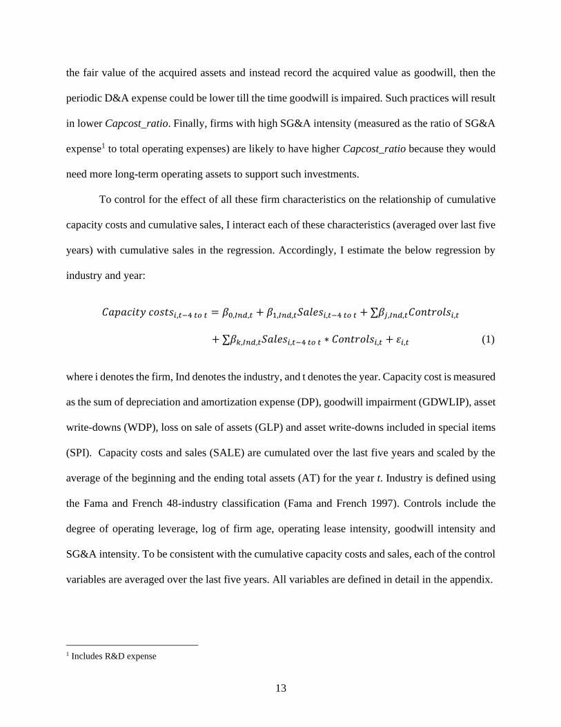
To control for the effect of all these firm characteristics on the relationship of cumulative

capacity costs and cumulative sales, I interact each of these characteristics (averaged over last five

years) with cumulative sales in the regression. Accordingly, I estimate the below regression by

industry and year:

𝐶𝑎𝑝𝑎𝑐𝑖𝑡𝑦 𝑐𝑜𝑠𝑡𝑠𝑖,𝑡−4 𝑡𝑜 𝑡 = 𝛽0,𝐼𝑛𝑑,𝑡 + 𝛽1,𝐼𝑛𝑑,𝑡𝑆𝑎𝑙𝑒𝑠𝑖,𝑡−4 𝑡𝑜 𝑡 + ∑𝛽𝑗,𝐼𝑛𝑑,𝑡𝐶𝑜𝑛𝑡𝑟𝑜𝑙𝑠𝑖,𝑡

+ ∑𝛽𝑘,𝐼𝑛𝑑,𝑡𝑆𝑎𝑙𝑒𝑠𝑖,𝑡−4 𝑡𝑜 𝑡 ∗ 𝐶𝑜𝑛𝑡𝑟𝑜𝑙𝑠𝑖,𝑡 + 𝜀𝑖,𝑡 (1)

where i denotes the firm, Ind denotes the industry, and t denotes the year. Capacity cost is measured

as the sum of depreciation and amortization expense (DP), goodwill impairment (GDWLIP), asset

write-downs (WDP), loss on sale of assets (GLP) and asset write-downs included in special items

(SPI). Capacity costs and sales (SALE) are cumulated over the last five years and scaled by the

average of the beginning and the ending total assets (AT) for the year t. Industry is defined using

the Fama and French 48-industry classification (Fama and French 1997). Controls include the

degree of operating leverage, log of firm age, operating lease intensity, goodwill intensity and

SG&A intensity. To be consistent with the cumulative capacity costs and sales, each of the control

variables are averaged over the last five years. All variables are defined in detail in the appendix.

1 Includes R&D expense

14

Finally, annual maintenance capex is estimated using the following equation:

𝑀𝑎𝑖𝑛𝑡𝑒𝑛𝑎𝑛𝑐𝑒 𝑐𝑎𝑝𝑒𝑥𝑖,𝑡 = (𝐶𝑎𝑝𝑎𝑐𝑖𝑡𝑦 𝑐𝑜𝑠𝑡𝑠𝑖,𝑡−4 𝑡𝑜 𝑡

𝑆𝑎𝑙𝑒𝑠𝑖,𝑡−4 𝑡𝑜 𝑡) ∗ 𝑆𝑎𝑙𝑒𝑠𝑖,𝑡, (2)

where 𝐶𝑎𝑝𝑎𝑐𝑖𝑡𝑦 𝑐𝑜𝑠𝑡𝑠𝑖,𝑡−4 𝑡𝑜 𝑡 is computed using the following equation:

𝐶𝑎𝑝𝑎𝑐𝑖𝑡𝑦 𝑐𝑜𝑠𝑡𝑠𝑖,𝑡−4 𝑡𝑜 𝑡 = ��0,𝐼𝑛𝑑,𝑡 + ��1,𝐼𝑛𝑑,𝑡𝑆𝑎𝑙𝑒𝑠𝑖,𝑡−4 𝑡𝑜 𝑡 + ∑��𝑗,𝐼𝑛𝑑,𝑡𝐶𝑜𝑛𝑡𝑟𝑜𝑙𝑠𝑖,𝑡

+ ∑��𝑘,𝐼𝑛𝑑,𝑡𝑆𝑎𝑙𝑒𝑠𝑖,𝑡−4 𝑡𝑜 𝑡 ∗ 𝐶𝑜𝑛𝑡𝑟𝑜𝑙𝑠𝑖,𝑡 (3)

The intercept in equation (3) can be interpreted as an approximation of the industry-average

technology obsolescence cost over the last five years. Therefore, the predicted cumulative capacity

costs incorporate the costs required to keep pace with the technological developments taking place

in an industry over time.

The above estimation procedure allows the estimated cumulative capacity costs to capture both

total wear and tear costs and technological obsolescence costs incurred over the last five years,

which are required to generates sales over the same period. Therefore, annual maintenance cost

gives a better estimate of the true capacity costs needed to maintain the current year revenues. This

estimate could be underestimated because the inputs to the model are historical costs and the

current replacement costs could be higher due to inflation. However, this estimate is a better

approximation of the true capacity costs compared to D&A expense as it captures industry-average

technological obsolescence costs also.

4. Data and Sample Statistics

4.1 Data

My sample consists of all firms that are incorporated in the U.S., have common shares

trading on NYSE, Amex, or NASDAQ, and have all the required data available on CRSP monthly

15

return files and Compustat annual files. My sample period starts from 1974 because data on

operating leases was not available before this year. The sample ends in 2016 because I need the

next three years’ data to compute future earnings, write-downs, and investments. To compute my

measure of maintenance capex, I require each firm-year in the sample to have accounting data

available on Compustat for the past five years. I exclude the financial services industry (industry

number 44 to 47 using the Fama and French 48-industry classification) as firms in these industries

differ from firms in other industries in their cost structures and business models. I also exclude the

category called “almost nothing” (industry number 48) because of the difficulty in interpreting the

results in an industry context. Further, to reduce the influence of very small firms, I also exclude

firms with negative book equity, stock price less than $1 and have less than $10 million of sales.

4.2 Sample Statistics

4.2.1 Capcost_ratio and Firm Characteristics

Panel A of Table 1 presents the descriptive statistics of Capcost_ratio, which is the ratio

of cumulative capacity costs to cumulative sales, and other firm characteristics that are used as

controls in the model for estimating maintenance capex. The mean (median) value of

Capcost_ratio is 0.07 (0.04) indicating that on an average, firms incur approximately 7 cents (4

cents) of capacity costs for 1 dollar of sales. Panel B of Table 1 shows that the capacity costs have

been steadily increasing from 4 cents for a dollar of sales in 1974 to 8 cents in 2016. Panel C of

Table 1 reports the time series average of yearly cross-sectional mean of Capcost_ratio by

industry. Precious Metals industry has the highest Capcost_ratio of around 21 cents. Petroleum

& Natural Gas has the next highest value of 19 cents following by Communication industry with

17 cents. Retail industry has one of the lowest values of Capcost_ratio at 3 cents. Firms in this

16

industry rely heavily on operating leases2. The average operating lease intensity of firms in this

industry is 19%, whereas the mean value for the entire sample is only 7%. Also, the business model

of retail firms has changed significantly in the recent times with the advent of ecommerce.

Table 1 also presents the descriptive statistics, time trend and industry mean of the firm

characteristics. Dol_5y is the degree of operating leverage obtained using firm specific time series

regressions of total operating costs on sales (Aboody, Levi and Weiss 2018). A high degree of

operating leverage indicates that a firm has a high proportion of fixed costs to variable costs. The

mean (median) value of Dol_5y for the entire sample is 0.07 (0.03). Operating leverage increases

monotonically over the sample period to an average of 0.14 in the year 2016. A potential

explanation for this time trend is the increase in outsourcing activities over the last two decades.

Among all the industries, pharmaceutical products, precious metals, and metals & mining have the

highest operating leverage. Once again retail industry has one of the lowest operating leverage at

0.03. Opl_intst_5y is the ratio of operating leases to total assets averaged over the last five years.

The mean (median) value for the entire sample is 0.06 (0.03). Operating lease intensity also has

steadily increased over the years from 0.01 in 1974 to 0.07 in 2016. Some of the industries with

high operating lease intensity are Retail (0.19), Restaurants, Hotels, Motels (0.18), Personal

services (0.13) and Transportation (0.10). Gdw_intst_5y is the ratio of goodwill to total assets

averaged over the last five years. The mean (median) value for the entire sample is 0.05(0). The

first year where goodwill intensity is non-zero is 1988. Very few firms booked goodwill on their

balance sheets in that year. Goodwill intensity increased significantly after the release of SFAS

2 I did not include rental expense on operating leases in the capacity costs.

17

1413 and SFAS 1424 in 2001 reaching an average of 0.14 in 2016. This shows that acquisition led

growth has become more prominent in the latter part of the sample period. Sga_intst_5y is the ratio

of SG&A expense to total operating costs averaged over the last five years. The mean (median) is

0.22 (0.19). This ratio has also increased monotonically over the sample period from 0.17 in 1974

to 0.25 in 2016 (Enache and Srivastava 2018).

Each of the firm characteristics described above could influence the relationship between

capacity costs and sales. Panel D of Table 1 reports the results of univariate and multivariate

regressions of these characteristics on Capcost_ratio. The coefficient on the degree of operating

leverage is positive and significant, which is consistent with my expectation that firms with higher

operating leverage have higher proportion of fixed costs to variable cost and hence higher capacity

costs. The coefficient on firm age is negative and significant. This indicates that older firms have

lower capacity costs. Older firms tend to be larger and in the mature stage of its life cycle. Hence

one would expect such firms to benefit from economies of scale and have lower capacity costs.

The coefficient on operating lease intensity is negative and significant confirming that firms with

higher reliance on operating leases will have relatively fewer assets on the balance sheet and hence

lower capacity costs (rental expense is excluded from capacity costs). The coefficients on goodwill

intensity and SG&A intensity are not significant both in univariate and multivariate regressions.

However, I retain them in the model to estimate maintenance capex.

3 SFAS 141 eliminated the alternative pooling-of-interests method of accounting for acquisitions. The popularity

of pooling stemmed largely from the fact that it did not require the recognition of goodwill and the associated

amortization charges. Post this rule, managers must recognize goodwill. 4 Prior to the release of SFAS 142 in 2001, APB Opinion No. 17 governed the accounting for goodwill (AICPA

1970). APB 17 required goodwill to be amortized to operating income over its estimated useful life, subject to a

maximum life of 40 years.

18

4.2.2 Maintenance CapEx

Table 2 Panel A reports the descriptive statistics for the estimated maintenance capex.

Mcap_ratio is the ratio of estimated annual maintenance capex to annual sales. The mean (median)

of Mcap_ratio is 0.067 (0.045). The first quartile value is 0.028 and third quartile value is 0.075.

To put this value in perspective, the mean (median) value of Dp_ratio (ratio of reported D&A

expense to sales) is 0.053 (0.034). Therefore, the mean (median) value of Underdep_ratio

(difference between estimated maintenance capex and D&A expense divided by annual sales) is

0.013 (-0.003). In percentage terms, the median firm seems to be under-depreciating by 25% of

the reported D&A expense.

Table 2 Panel B reports the descriptive statistics for the estimated maintenance capex and

under-depreciation by size. The mean (median) of Mcap_ratio is 0.059 (0.043) for small firms,

0.07 (0.049) for medium firms and 0.076 (0.054) for large firms. Compared to the estimated

maintenance capex value, the recognized D&A expense of a median firm is lower by 32% in the

small size category, 26% in the medium size category and 19.6% for the large size category.

Table 2 Panel C reports the time trend of estimated maintenance capex and under-

depreciation. The mean (median) value of Mcap_ratio increased from 0.038 (0.027) in 1974 to

0.081 (0.055) in 2016. The percentage of under-depreciation is high for years during and

immediately after a crisis mainly because of the incidence of impairments and write-downs during

the crisis period. Since the estimation procedure includes the write-downs and impairments for the

last five years, one would observe higher estimated maintenance capex when the last five years

overlap with the crisis period. The higher maintenance capex reflects the fact that a crisis year

increases the rate of technological obsolescence and renders old assets unproductive. As a result,

19

firms need to replace these assets with new assets that are equipped with new technology. Any

firm that delays this process is more likely to lose out to competition.

Table 2 Panel D reports the time series average of yearly cross-sectional mean (median) values of

estimated maintenance capex and under-depreciation for different industries. Some of the major

industries with the percentage of under-depreciation above the sample median (25%) are

Pharmaceutical Products (47.5%), Construction (63.5%), Healthcare and Medical equipment

(39%), Business Services (59.4%), Computers (56%), Electronic equipment (49.6%) and

Wholesale (52%). These are the industries which experienced a higher rate of technological

obsolescence and disruption to their business during the sample period. My measure of

maintenance capex and under-depreciation suggests that firms in these industries should reduce

their current estimates of useful lives for their long-term operating assets, such that their reported

D&A expense can reflect timely information of capacity costs needed for every dollar of sale

generated.

5. Validation Using Future Write-offs and Future Earnings

In this section, I validate my measure of maintenance capex by showing that firms that do

not recognize sufficient expense for maintenance capex will have to write off their assets in the

future. To do that, I first compute the amount of under-depreciation, which is the difference

between the estimated maintenance capex and the recognized D&A expense. A positive value of

under-depreciation indicates that the D&A expense in the income statement understates the true

capacity costs expended to generate the current year revenues, and the current period earnings are

therefore overstated. Specifically, I examine whether the level of under-depreciation is associated

with future write-offs and hence lower future earnings over the next one to three years.

20

5.1 Future Write-offs

Matching principle requires that the expense related to the usage of all capitalized long-

term operating assets should be recognized in the same period in which the related revenues are

earned. However, these costs are less timely due to managers’ discretion in allocating them across

time periods. Managers tend to postpone these costs to future periods in order to show higher

income in the current period. If my measure of under-depreciation is a good proxy for such

postponement of capacity costs recognition, then we should observe larger write-offs for the under-

depreciating firms in the future. To test this, I examine the following tobit regression:

𝐹𝑢𝑡𝑢𝑟𝑒_𝑤𝑟𝑖𝑡𝑒𝑜𝑓𝑓𝑠𝑖,𝑡+𝑘 = 𝛽0 + 𝛽1𝑈𝑛𝑑𝑒𝑟𝑑𝑒𝑝𝑖,𝑡 + 𝛽2𝑊𝑟𝑖𝑡𝑒𝑜𝑓𝑓𝑖,𝑡 + ∑𝛽𝑗𝐶𝑜𝑛𝑡𝑟𝑜𝑙𝑠𝑖,𝑡 + 𝜀𝑖,𝑡+𝑘

(4)

Write-offs in the above equation are computed as the sum of goodwill impairment

(GDWLIP), asset write-downs (WDP), loss on sale of assets (GLP) and asset write-downs included

in special items (SPI) scaled by beginning total assets. I use four proxies for future write-offs

including the write-offs for year t+1, t+2, and t+3, and excess future write-off computed as the

average of the next three years’ write-offs minus the current year write-offs. Consistent with Hanna

and Vincent (1996) , I control for current write-offs, log of sales, industry-adjusted book-to-market

ratio of the current year, mean change in book-to-market ratio over the last five years, mean change

in the firm’s industry median book-to-market ratio over the last five years, mean change in return-

on-assets ratio over the last five years, mean change in the firm’s industry median return-on-assets

ratio over the last five years, mean of the annual median percentage sales growth of all firms in

the same industry as the firm over the last five years, goodwill intensity, number of years in which

the firm reported write-offs in the last five years, cumulative abnormal returns over the last 12

months ending four months after the fiscal year end (to capture investors’ reaction to the write-

21

offs information in the annual report), cumulative abnormal returns over the last five years ending

four months after the fiscal year end of year t-1. The main variable of interest is Underdep (under-

depreciation scaled by average of total assets). If this variable is a good estimate of the true level

of under-depreciation, then I expect a positive coefficient for 𝛽1.

Panel B of Table 3 reports the results of Equation (4). As expected, Underdep is positively

associated with future write-offs. The coefficient on Underdep is positive and significant when the

dependent variable is write-offs in year t+2 (t-statistic of 3.87), write-offs in year t+3 (t-statistic of

7.35) and change in average write-offs for next three years relative to that of the current year (t-

statistic is 7.03). However, the coefficient on Underdep is positive but not significant (t-statistic

of 1.24) when the dependent variable is next year (t+1) write-offs. This shows that a higher level

of under-depreciation in the current year is associated with increased write-downs in the future.

These results are obtained even after controlling for the market’s expectation of firm’s future write-

offs, historical firm performance, and the firm’s own history of write-offs. The sign of the

coefficients on all the controls are consistent with those in Hanna and Vincent (1996).

5.2 Future Earnings

Having documented the effect of under-depreciation on future write-offs, I further verify

that under-depreciation is also associated with negative future earnings. I examine this relationship

using the following equation:

𝐹𝑢𝑡𝑢𝑟𝑒_𝐸𝑎𝑟𝑛𝑖𝑛𝑔𝑠𝑖,𝑡+𝑘 = 𝛽0 + 𝛽1𝑈𝑛𝑑𝑒𝑟𝑑𝑒𝑝𝑖,𝑡 + 𝛽2𝐸𝑎𝑟𝑛𝑖𝑛𝑔𝑠𝑖,𝑡 + ∑��𝑗𝐶𝑜𝑛𝑡𝑟𝑜𝑙𝑠𝑖,𝑡

+ 𝐼𝑛𝑑𝑢𝑠𝑡𝑟𝑦𝐹𝐸 + 𝑌𝑒𝑎𝑟𝐹𝐸 + 𝜀𝑖,𝑡+𝑘 (5)

I use four proxies for future earnings including the earnings for year t+1, t+2, and t+3, and

excess future earnings computed as the difference between the average of the next three years’

earnings and the current year earnings. Earnings is defined as income before extraordinary items

22

(IB) scaled by average total assets. I control for current earnings scaled by average total assets, log

of market value of equity, R&D expense scaled by average total assets, SG&A expense scaled by

average total assets, leverage, current earnings growth, and an indicator for negative earnings in

the current year. The main variable of interest is Underdep (under-depreciation scaled by average

of total assets). If this variable is a good estimate of the true level of under-depreciation for the

current year, then I expect a negative coefficient for 𝛽1.

Table 4 panel B reports the results of Equation (5). The t-statistics are reported by clustering

errors by industry and year. As can be seen in this table, Underdep is negatively associated with

future earnings. In particular, the coefficient on Underdep is negative and significant for year t+2

(t-statistic is -5.42) and for year t+3 (t-statistics is -5.59). However, the coefficient on Underdep is

negative but not significant (t-statistic is -1.12) for year t+1. The relationship also holds when the

dependent variable is excess future earnings, computed as the difference between the average of

earnings for the next three years and the current year earnings.

6. Under-depreciation and Future Stock Returns

In this section, I test whether the information contained in my measure of estimated

maintenance capex is priced by investors. Specifically, I test the implications of under-depreciation

for future stock returns.

If the estimated under-depreciation is not associated with future excess stock returns after

controlling for the known determinants of the cross section of returns, then the inference could be

either one of the following. First, it is possible that investors price the stocks as if the periodic

capacity costs are irrelevant. Proponents of EBITDA, for example, may think that periodic

capacity costs do not affect cash flows and therefore should not have any implications for

valuation. Second, it could be that the information in the under-depreciation measure has already

23

been priced. Lastly, it may suggest that my measure is not a good estimate of the true capacity

cost.

On the other hand, if the under-depreciation measure is negatively correlated with future

excess stock returns, then we can infer that the measure is a good estimate of the true capacity cost,

and that investors do not price this information. To test this, I examine the following Fama-

Macbeth regression:

𝐹𝑢𝑡𝑢𝑟𝑒_𝑅𝑒𝑡𝑢𝑟𝑛𝑠𝑖,𝑡+1 = 𝛽0 + 𝛽1𝑈𝑛𝑑𝑒𝑟𝑑𝑒𝑝_𝑖𝑛𝑑𝑎𝑑𝑗𝑖,𝑡 + ∑𝛽𝑗𝐶𝑜𝑛𝑡𝑟𝑜𝑙𝑠𝑖,𝑡 + 𝜀𝑖,𝑡+1 (6)

where future returns are measured in two different ways: monthly excess returns or annual excess

returns. Monthly excess returns are obtained by subtracting the risk-free return from each stock’s

raw return. Annual buy and hold excess returns are obtained by subtracting annual buy and hold

risk free return from each stock’s annual buy and hold raw return. I control for log of market

capitalization, log of book-to-market ratio, momentum, operating profitability, and new

investment in long-term operating assets (Fama and French 2015). The main independent variable,

Underdep_indadj, is defined as firm-level under-depreciation minus the industry median. I expect

the coefficient 𝛽1 to be negative, which would indicate that stocks with higher industry adjusted

under-depreciation in the current year experience negative abnormal returns in the future.

Return tests are conducted by mapping monthly stock returns from CRSP with annual

accounting data from Compustat. I map them using both annual and monthly rebalancing methods.

In annual rebalancing, the monthly returns starting from May of year t to April of year t+1 are

mapped to the independent variable of interest, Underdep_indadj, for the fiscal year ending in year

t-1. The advantage of this approach is that it yields an abnormal return measure that accurately

represents investor’s experience. The disadvantage of this approach is that it is more sensitive to

the problem of cross-sectional dependence among sample firms and a poorly specified asset

24

pricing model (Lyon, Barber and Tsai 1999). In monthly rebalancing, each monthly return is

mapped to Underdep_indadj for the nearest available fiscal year with a gap of four months5. The

advantage of this approach is that it controls well for cross-sectional dependence among sample

firms and is generally less sensitive to a poorly specified asset pricing model. The disadvantage of

this approach is that it yields an abnormal return measure that does not precisely measure investor

experience.

Table 5 reports the results from annual and monthly Fama-MacBeth cross-sectional

regressions (Fama and Macbeth 1973) of individual stocks’ excess returns on lagged

Underdep_indadj. Panel A of Table 5 reports the results of annual return regression where the

dependent variable is the buy and hold excess returns accumulated from the month of May of year

t to April of year t+1. For each return year, the buy and hold excess returns is mapped to the

independent variable of interest, Underdep_indadj, for the fiscal year ending in year t-1. The

coefficient on Underdep_indadj is negative and significant (t-statistic is -3.71) after controlling

for size, book-to-market, operating profitability and investment. The point estimate on

Underdep_indadj range from -0.439 (without controls) to -0.368 (with controls).

Panel B of Table 5 reports the results of monthly return regression where the dependent

variable is the monthly excess return. The independent variable, Underdep_indadj, is updated only

once a year in the month of April using the data for the fiscal year ending in year t-1. Even here,

the coefficient is negative and significant. The t-statistic is -4.66 without controls and -4.40 after

adding the controls. The point estimate on Underdep_indadj ranges from -0.035 (without controls)

to -0.032 (with controls). Panel C of Table 5 reports the results of monthly return regression where

the dependent variable is the monthly excess return. The independent variable, Underdep_indadj,

5 I assume that accounting data are publicly available 4 months after the fiscal year end.

25

is updated every month using the data from the nearest fiscal year with a gap of four months. As

with the annual rebalancing approach, the monthly rebalancing approach also shows that the

coefficient is negative and significant with the t-statistic of -4.36 without controls and -4.18 with

controls. The point estimate on Underdep_indadj ranges from -0.033 (without controls) to -0.031

(with controls).

Given that my estimate of under-depreciation predicts negative future returns, I further

examine whether a trading strategy of going long on highest decile portfolio and short on lowest

decile portfolio of under-depreciation can generate negative returns. Specifically, every month I

assign firms to deciles based on the level of Underdep_indadj. I then compute monthly equal-

weighted (EW) and value-weighted (VW) portfolio returns for each decile portfolio for the period

of May 1974 to December 2016. The zero-investment portfolio return for each calendar year is

then estimated by the difference between the Jensen’s alphas of the highest-ranked and lowest-

ranked portfolios. Because alphas are calculated using monthly returns, they are annualized by

multiplying by 12. Means and statistical significance of the zero-investment portfolio returns for

each calendar year from 1974 to 2016 are presented in Table 6. The zero-investment portfolio

alphas formed based on the level of industry adjusted under-depreciation are negative for more

than 70% of the years (not tabulated). Table 6 Panel A reports the average annualized zero-

investment portfolio returns, where portfolios are assigned using annual rebalancing method. The

average values of equal-weighted (value-weighted) raw returns are -4.38% (-3.60%). The average

values of equal-weighted (value-weighted) alphas are -3.97% (-3.35%) and -3.72% (-2.89%) in

the Carhart four factor model and the Fama and French five factor model, respectively. All these

returns are statistically significant at 1% level with absolute value of t-statistics above 3. Table 6

Panel B reports similar results when portfolios are assigned using monthly rebalancing method.

26

The average values of equal-weighted (value-weighted) raw returns are -4.36% (-3.22%). The

average values of equal-weighted (value-weighted) alphas are -4.21% (-3.25%) and -4.11% (-

2.77%) in the Carhart four factor model and the Fama and French five factor model, respectively.

These returns are also statistically significant at 1% level with absolute value of t-statistics above

3.

Taken together, all the above results suggest that investors do not price the information in

under-depreciation, possibly because they do not have information on the true capacity cost and

how much the capacity cost differs from the reported D&A expense.

7. Implications of Maintenance CapEx for Future Investments

7.1 Under-investment and Future Investments

In this section, I examine whether my measure of maintenance capex can explain firms’

future abnormal investments in long-term operating assets. Specifically, I use the construct of

under-investment, measured as the difference between the estimated maintenance capex and the

actual investments made by the firm in long-term operating assets, to test whether any shortfall in

expenditures in the current year can predict abnormal investment expenditures in the future years.

Maintenance capex is the minimum amount of capital expenditure required to be replaced

to maintain the current operations. If the firm does not invest at least to this extent, then it will be

compelled to increase its investments in the future to sustain its operations. If my measure of

maintenance capex is a good estimate of the actual capacity costs, then I expect firms with higher

levels of under-investment to increase their future investments. I examine this implication of

under-investment using the following equation:

𝐹𝑢𝑡𝑢𝑟𝑒_𝐼𝑛𝑣𝑒𝑠𝑡𝑚𝑒𝑛𝑡𝑠𝑖,𝑡+𝑘 = 𝛽0 + 𝛽1𝑈𝑛𝑑𝑒𝑟𝑖𝑛𝑣𝑒𝑠𝑡𝑖,𝑡 + ∑𝛽𝑗𝐶𝑜𝑛𝑡𝑟𝑜𝑙𝑠𝑖,𝑡 + 𝜀𝑖,𝑡+1 (7)

27

I use four proxies for future investments including investments made in year t+1, t+2, and

t+3, and excess investments computed as the difference between the average of the next three

years’ investments and the current year investment. Here I refer to investments as the annual

change in long-term operating assets, excluding any non-transaction accruals (Lewellen and

Resutek 2016). I control for current investments, leverage, log of market value of equity, log of

firm age, book-to-market ratio, and amount of cash (CHE) scaled by total assets. The main variable

of interest is Underinvest (Under-investment scaled by average of total assets). If this variable is a

good estimate of the level of under-investment, then I expect a positive coefficient for 𝛽1. The

positive coefficient would imply that firms must invest more in the future to compensate for the

under-investment in the current period.

Panel B of Table 7 reports the results of equation 6. The t-statistics are reported by

clustering errors by industry and year. As can be seen in this table, Underinvest is positively

associated with future investments. In particular, the coefficient on Underinvest is positive and

significant when the dependent variable is investment in year t+1 (t-statistic is 12.03), investment

in year t+2 (t-statistic is 8.58) and investments in year t+3 (t-statistic is 6.70). The relationship also

holds when the dependent variable is excess future investments, computed as the difference

between the average investment over the next three years and the current year investment. For

robustness, I also check whether this relationship holds when the dependent variables are replaced

by abnormal investment. For each future year, abnormal investment is computed as the difference

between the investment in that year and the average investment over the last three years (Titman

et al., 2004). Panel C of Table 7 reports the results. The coefficient on Underinvest continues to be

positive and significant when the dependent variable is abnormal investment in year t+1 (t-

statistics is 8.85), abnormal investment in year t+2 (t-statistics is 11.89),and abnormal investment

28

in year t+3 (t-statistics is 8.58). These results are consistent with the idea that if firms under-invest

relative to the estimated maintenance capex in the current year, then they will have to increase

their investments in future to sustain their current operations.

7.2 Re-examining the Relationship Between Investment & Future Stock Returns

In this section, I examine whether the estimated maintenance capex measure can partially

explain the negative relationship between investment and future stock returns reported in prior

literature.

The information content of long-term assets on the balance sheet and its implications for

future stock has been extensively studied in both the finance and accounting literatures. The

finance literature focuses on the additions to the long-term asset portfolio through capital

investments. Several empirical studies in this literature show a significantly negative relationship

between capital investment (and asset growth) and future abnormal stock returns, which is

popularly known as the investment anomaly. Cooper et al. (2008) show that corporate events

related with asset expansion tend to be followed by periods of abnormally low returns. Researchers

have tried to explain this relationship using both behavioral and risk-based explanations. Titman

et al. (2004) suggest that investors do not fully understand managers’ bias towards empire building

and hence overreact to the investment decision. The negative future abnormal return is then a

correction to the initial overreaction. While the behavioral explanation suggests market mispricing,

the risk-based explanation suggests a reduction in expected returns following the resolution of

uncertainty in investment. This explanation is derived from real-options models, which predict a

decline in systematic risk following the exercise of growth options. Consistent with this

explanation, Cooper and Priestley (2011) show that firms’ systematic risk falls during periods of

high investment (asset growth). Prior accounting studies also examine this section of the balance

29

sheet as long-term operating accruals and found similar implications for future abnormal returns.

Fairfield and Whisenant (2003) argue that both conservative accounting principles and diminishing

marginal returns to increased investment tend to reduce future profitability.

While I do not contest the above explanations, I posit that the negative relationship between

investment and future stock returns can partly be explained by the inability of investors to

understand how much of the current investment is for maintenance and how much of it is for

growth. I test this hypothesis using the following equation.

𝐹𝑢𝑡𝑢𝑟𝑒_𝑅𝑒𝑡𝑢𝑟𝑛𝑠𝑖,𝑡+1 = 𝛽0 + 𝛽1𝐼𝑛𝑣𝑎𝑐𝑐𝑖,𝑡 + 𝛽1𝑀𝑐𝑎𝑝𝑖,𝑡 + 𝛽1𝐼𝑛𝑣𝑎𝑐𝑐𝑖,𝑡 ∗ 𝑀𝑐𝑎𝑝𝑖,𝑡

+∑𝛽𝑗𝐶𝑜𝑛𝑡𝑟𝑜𝑙𝑠𝑖,𝑡 + 𝜀𝑖,𝑡+1 (8)

where future returns are monthly excess returns measured by subtracting risk-free return from the

stocks’ raw returns. I control for other important determinants of the cross-section of returns. This

includes log of market capitalization, log of book to market ratio, momentum, and operating

profitability. Mcap is the estimated maintenance capex scaled by average total assets and Invacc

is the total new investment added to long-term operating assets in the current year scaled by

average total assets.

Table 8 reports the results from monthly Fama-MacBeth cross-sectional regressions. Panel

A of Table 8 reports the results using annual rebalancing, where financial statement variables are

only updated once a year and Panel B of Table 8 reports the results using monthly rebalancing,

where financial statement variables are updated as and when they are available to the investor (four

months from the fiscal year end). Column (1) in both the panels is the baseline regression to

replicate the negative relationship between investment and future stock returns. Consistent with

prior literature, the coefficient (-0.012) on investment is negative and significant (t-statistic of -

5.80). In column (2), I interact investment with the reported D&A expense. The coefficient on the

30

interaction term is negative and significant at the 10% level. This shows that the negative

relationship between investment and future stock returns is more pronounced at higher levels of

D&A expense. In column (3), I interact investments with the estimated maintenance capex. The

coefficient on the interaction term is negative and significant at the 5% level, indicating that the

negative relationship of investment and future stock returns is also more pronounced at higher

levels of maintenance capex. Moreover, the coefficient in column (3) is -0.158, which is much

lower than the one in column (2) (-0.083). These results suggest that investors do not price current

investments after adjusting for the required maintenance capex.

8. Conclusion

The rate of technological development is rapidly increasing and is proving to be

particularly costly for businesses today. It is crucial that firms recognize the need to replace

technologically obsolete assets, record the related expense in a timely manner, and invest

accordingly to remain competitive. Ideally, managers should anticipate the capacity costs of long-

term operating assets due to technological obsolescence and incorporate that into D&A expense to

match with the related revenue generated. In reality, however, firms often record D&A expense

that do not capture the effect of technological changes. Such practice understates the actual

capacity cost required for a firm to sustain its current level of revenue and may give investors the

false impression that the firm could sustain its current level of profitability in the future.

In this paper, I propose a measure of maintenance capex that reflects the true capacity cost

required for a firm to sustain its current level of revenue. My measure has three features that makes

it a better estimate of capacity cost than the traditional D&A expense. First, it captures not only

the periodic wear and tear cost, but also the costs arising from the technological obsolescence of

long-term operating assets. Second, it takes into account the fact that the relationship between

31

capacity costs and sales varies by industry. Third, it incorporates the effect of firm characteristics,

such as a firm’s asset composition, cost structure, and life cycle, on the relationship between

capacity costs and sales. Using this measure, I identify under-depreciating firms that record D&A

expenses which are lower than maintenance capex.

I validate my measure by showing that under-depreciation is associated with future write-

offs and hence negative future earnings. In other words, if a firm does not recognize sufficient

D&A expense in the current period, it will ultimately have to record a write-off of the

technologically obsolete assets in some future period. The asset write-off will have a negative

impact on the firm’s future earnings. My measure can help investors anticipate future write-offs

and negative future earnings.

Moreover, I show that under-depreciation is associated with significantly negative future

stock returns. This confirms my hypothesis that investors may not realize that a firm’s earnings

are overstated when the firm fails to recognize the costs of technological obsolescence in its D&A

expense. Investors seem to have priced the stock assuming that the firm can sustain the same level

of earnings without incurring the related capacity costs and are negatively surprised in the future

period.

An alternative way to interpret the estimated capacity cost is that it proxies for the

minimum amount of capital expenditure required for a firm to replace outdated assets and remain

competitive. When compared to the actual amount of investment made by a firm, one can draw

inferences on whether the firm has invested enough to sustain its current revenue. One can also

observe the amount of actual investment in excess of the required investment, which can lead to

revenue growth beyond the current level. In additional tests, I show that under-investment is

positively associated with future investments. In other words, if a firm does not make sufficient

32

investments in the current period, it will have to increase its investment in the future period. I also

re-examine the negative relationship between asset growth and future stock return documented in

prior literature and find that this relationship is partly caused by investors’ inability to differentiate

maintenance versus growth capex.

In conclusion, my measure of maintenance capex can inform financial statement users

about the actual capacity cost required to sustain a firm’s current revenue and help them identify

under-depreciating firms that are likely to have future asset write-downs. It also enables investors

to distinguish between investments that are necessary to sustain a firm’s current level of

profitability versus the investments that could result in further expansion of a business.

33

Figure 1: Time Trend of Maintenance CapEx

Figure 1 exhibits the time trend for the cross-sectional median of DP_ratio (D&A expense divided by sales), Mcap_ratio (Estimated

Maintenance CapEx divided by sales) and Underdep_ratio (Difference between Maintenance CapEx and D&A expense divided by

sales).

0

.02

.04

.06

1974 1977 1980 1983 1986 1989 1992 1995 1998 2001 2004 2007 2010 2013 2016year

DP_ratio Mcap_ratio Underdep_ratio

34

Figure 2: Time Trend of Under-depreciation

Figure 2 exhibits the time trend for the cross-sectional median of Underdep_DP (Difference between Maintenance CapEx and D&A

expense divided by D&A expense), Underdep_OI (Difference between Maintenance CapEx and D&A expense divided by Operating

income) and Underdep_IB (Difference between Maintenance CapEx and D&A expense divided by Net Income).

60 %

0 %

20 %

20 %

40 %

40 %

60 %

1974 1977 1980 1983 1986 1989 1992 1995 1998 2001 2004 2007 2010 2013 2016year

Underdep_DP% Underdep_OI% Underdep_IB%

35

Table 1: Descriptive Statistics of Model Variables

This table presents descriptive statistics for the variables used in the model to estimate maintenance

capex. The sample period is from 1974 to 2016. All the variables are defined in the appendix.

Panel A reports the descriptive statistics for the full sample. Panel B reports the time trend in these

variables and Panel C reports the time series average of yearly cross sectional mean values of the

variables for Fama French 48 industries. Panel D reports the univariate and multivariate regression

of Capcost_ratio on firm characteristics. Year and Industry fixed effects are included and t-

statistics using robust standard errors that are clustered at year and industry level are presented in

parentheses below coefficient estimates. All continuous variables are winsorized annually at their

1st and 99th percentiles. *, **, and *** indicate two-tailed statistical significance at 10, 5, and 1

percent levels, respectively.

Panel A: Full Sample

N Mean Std dev First quartile Median Third quartile

Capcost_ratio 109252 0.07 0.09 0.02 0.04 0.07

Dol_5y 109252 0.07 0.22 -0.03 0.03 0.14

Age_5y 109252 18.21 12.5 8 15 25

Opl_intst_5y 109252 0.06 0.09 0.01 0.03 0.07

Gdw_intst_5y 109252 0.05 0.1 0 0 0.05

Sga_intst_5y 109252 0.22 0.17 0.1 0.19 0.31

Panel B: Time Trend from 1974 to 2016

Year Capcost_ratio Dol_5y Age_5y Opl_intst_5y Gdw_intst_5y Sga_intst_5y

1974 0.04 -0.01 12.31 0.01 0.00 0.17

1975 0.04 0.00 12.72 0.02 0.00 0.17

1976 0.04 0.00 13.15 0.03 0.00 0.17

1977 0.04 0.01 13.77 0.04 0.00 0.17

1978 0.04 0.02 13.96 0.04 0.00 0.17

1979 0.04 0.02 14.58 0.04 0.00 0.17

1980 0.04 0.02 15.21 0.04 0.00 0.17

1981 0.04 0.02 15.91 0.04 0.00 0.18

1982 0.04 0.01 16.66 0.04 0.00 0.18

1983 0.04 0.02 17.10 0.04 0.00 0.19

1984 0.04 0.03 17.26 0.04 0.00 0.19

1985 0.05 0.04 17.71 0.05 0.00 0.20

1986 0.05 0.06 17.09 0.05 0.00 0.21

1987 0.05 0.07 17.16 0.05 0.00 0.21

1988 0.06 0.06 17.41 0.06 0.01 0.21

1989 0.06 0.06 17.01 0.06 0.01 0.21

1990 0.06 0.05 17.24 0.06 0.02 0.21

36

1991 0.06 0.04 17.53 0.06 0.02 0.21

1992 0.06 0.04 17.91 0.06 0.03 0.21

1993 0.07 0.05 18.01 0.06 0.03 0.21

1994 0.07 0.06 18.00 0.06 0.04 0.22

1995 0.07 0.08 17.73 0.06 0.04 0.22

1996 0.07 0.10 17.45 0.06 0.04 0.22

1997 0.07 0.09 17.39 0.06 0.04 0.22

1998 0.07 0.09 17.52 0.07 0.05 0.22

1999 0.08 0.10 16.48 0.07 0.05 0.24

2000 0.08 0.09 17.13 0.07 0.05 0.24

2001 0.09 0.08 17.93 0.08 0.06 0.24

2002 0.10 0.08 18.11 0.08 0.07 0.25

2003 0.11 0.09 18.27 0.08 0.08 0.26

2004 0.10 0.10 19.16 0.08 0.09 0.26

2005 0.09 0.11 19.96 0.08 0.10 0.25

2006 0.07 0.13 20.54 0.08 0.11 0.25

2007 0.07 0.12 20.91 0.08 0.12 0.25

2008 0.07 0.10 22.12 0.07 0.12 0.24

2009 0.08 0.10 22.28 0.07 0.12 0.25

2010 0.08 0.10 22.80 0.07 0.12 0.24

2011 0.08 0.11 23.71 0.07 0.12 0.24

2012 0.08 0.12 24.24 0.07 0.12 0.24

2013 0.08 0.13 24.59 0.07 0.12 0.25

2014 0.07 0.14 24.94 0.07 0.13 0.25

2015 0.08 0.14 25.36 0.07 0.13 0.25

2016 0.08 0.14 25.47 0.07 0.14 0.25

Panel C: Industry Averages Using Fama and French 48-Industry Classification

Name Capcost

_ratio

Dol_

5y

Age_

5y

Opl_intst

_5y

Gdw_intst

_5y

Sga_intst

_5y

Agriculture 0.06 0.07 16.78 0.04 0.05 0.15

Food Products 0.03 0.03 23.10 0.03 0.06 0.19

Candy & Soda 0.03 -0.02 16.92 0.03 0.00 0.28

Beer & Liquor 0.05 0.00 20.09 0.02 0.02 0.25

Tobacco Products 0.02 -0.05 19.61 0.01 0.00 0.22

Recreation 0.04 0.07 17.12 0.04 0.04 0.28

Entertainment 0.10 0.10 14.58 0.07 0.05 0.17

Printing and Publishing 0.06 0.05 22.61 0.05 0.11 0.32

Consumer Goods 0.03 0.05 22.39 0.05 0.05 0.30

Apparel 0.02 0.05 19.66 0.09 0.04 0.25

37

Healthcare 0.06 0.05 11.43 0.09 0.11 0.17

Medical Equipment 0.06 0.10 14.47 0.04 0.06 0.40

Pharmaceutical Products 0.08 0.21 15.88 0.04 0.03 0.38

Chemicals 0.05 0.06 23.49 0.03 0.05 0.20

Rubber and Plastic Products 0.05 0.04 18.18 0.04 0.06 0.19

Textiles 0.04 0.04 19.62 0.04 0.04 0.15

Construction Materials 0.04 0.07 22.40 0.03 0.05 0.17

Construction 0.03 0.05 17.88 0.03 0.04 0.11

Steel Works Etc 0.04 0.11 22.04 0.01 0.04 0.10

Fabricated Products 0.04 0.04 19.28 0.02 0.05 0.14

Machinery 0.04 0.09 21.00 0.03 0.06 0.23

Electrical Equipment 0.04 0.08 21.09 0.03 0.06 0.24

Automobiles and Trucks 0.04 0.05 22.17 0.02 0.05 0.14

Aircraft 0.04 0.09 29.18 0.03 0.08 0.14

Shipbuilding, Railroad

Equipment 0.04 0.02 17.00 0.02 0.03 0.10

Precious Metals 0.21 0.20 16.74 0.01 0.00 0.17

Non-Metallic & Metal

Mining 0.09 0.16 19.88 0.02 0.02 0.11

Coal 0.10 0.13 11.64 0.02 0.01 0.07

Petroleum and Natural Gas 0.19 0.14 17.81 0.02 0.01 0.13

Utilities 0.09 -0.06 31.56 0.00 0.00 0.01

Communication 0.17 0.04 15.43 0.04 0.06 0.21

Personal Services 0.07 0.02 15.30 0.13 0.08 0.24

Business Services 0.08 0.08 12.51 0.09 0.09 0.29

Computers 0.07 0.10 14.04 0.06 0.06 0.35

Electronic Equipment 0.07 0.12 16.82 0.04 0.04 0.27

Measuring and Control

Equipment 0.05 0.11 18.25 0.04 0.06 0.35

Business Supplies 0.05 0.05 24.16 0.03 0.05 0.18

Shipping Containers 0.05 0.03 21.10 0.02 0.07 0.12

Transportation 0.07 0.04 18.31 0.10 0.03 0.08

Wholesale 0.02 0.04 16.97 0.05 0.05 0.18

Retail 0.03 0.03 16.98 0.19 0.04 0.26

Restaurants, Hotels, Motels 0.06 0.03 15.65 0.18 0.03 0.13

38

Panel D: Capcost_ratio vs Firm Characteristics

Dependent variable: Capcost_ratio

Intercept 0.062*** 0.097*** 0.068*** 0.066*** 0.059*** 0.089***

(109.75) (10.29) (56.03) (101.60) (12.96) (9.20)

Dol_5y 0.051*** 0.044***

(6.44) (6.56)

Age_5y -0.012*** -0.010***

(-3.30) (-3.08)

Opl_intst_5y -0.051** -0.063***

(-2.37) (-2.78)

Gdw_intst_5y -0.015 -0.006

(-0.92) (-0.40)

Sga_intst_5y 0.030 0.020

(1.42) (1.12)

Industry FE Yes Yes Yes Yes Yes Yes

Year FE Yes Yes Yes Yes Yes Yes

Adj.R-squared 0.279 0.274 0.266 0.265 0.267 0.288

N 109252 109252 109252 109252 109252 109252

39

Table 2: Descriptive Statistics of Model Output

This table presents descriptive statistics for estimated maintenance capex as a ratio of sales

(Mcap_ratio), and under depreciation as a ratio of sales (Underdep_ratio). Under depreciation is

measured as the difference between maintenance capex and depreciation & amortization (D&A)

expense. Underdep (%) is the difference between estimated maintenance capex and D&A expense

divided by D&A expense. This measures the extent of under depreciation comparing the capacity

costs possibly incurred by the firm and what is being reported in terms of D&A expense. For

comparison, the table also provides descriptive statistics of Capcost_ratio and Dp_ratio. The

sample period is from 1974 to 2016. All the variables are defined in the appendix. Panel A reports

the descriptive statistics for the full sample. Panel B reports time series average of yearly cross

sectional mean and median values of the variables for small, medium, and large size groups

classified using NYSE size breakpoints. Panel C reports the time trend in these variables and Panel

D reports the time series average of yearly cross sectional mean values of the variables for Fama

French 48 industries.

Panel A: Descriptive Statistics

N Mean Std dev First quartile Median Third quartile

Capcost_ratio 109252 0.065 0.087 0.023 0.040 0.073

Dp_ratio 109252 0.053 0.063 0.020 0.034 0.060

Mcap_ratio 109252 0.067 0.073 0.028 0.045 0.075

Underdep_ratio 109252 0.013 0.050 -0.003 0.007 0.022

Underdep (%) 109252 0.645 1.404 -0.085 0.251 0.825

Panel B: Descriptive Statistics by Size Group

Size Capcost_ratio Dp_ratio Mcap_ratio Underdep_ratio Underdep (%)

Mean Median Mean Median Mean Median Mean Median Mean Median

Small 0.061 0.038 0.047 0.031 0.059 0.043 0.011 0.009 0.740 0.322

Medium 0.067 0.042 0.056 0.037 0.070 0.049 0.012 0.009 0.588 0.260

Large 0.070 0.049 0.062 0.043 0.076 0.054 0.012 0.008 0.455 0.196

Panel C: Time Trend from 1974 to 2016

Year Capcost_ratio Dp_ratio Mcap_ratio Underdep_ratio Underdep (%)

Mean Median Mean Median Mean Median Mean Median Mean Median

1974 0.038 0.026 0.037 0.025 0.038 0.027 0.004 0.003 0.327 0.155

1975 0.037 0.025 0.036 0.024 0.038 0.027 0.002 0.002 0.272 0.111

1976 0.036 0.025 0.035 0.024 0.037 0.027 0.002 0.003 0.295 0.123

1977 0.036 0.024 0.034 0.023 0.036 0.027 0.002 0.003 0.304 0.133

1978 0.036 0.024 0.034 0.023 0.036 0.027 0.002 0.003 0.318 0.119

1979 0.036 0.024 0.034 0.023 0.036 0.027 0.002 0.003 0.321 0.120

1980 0.035 0.024 0.034 0.023 0.036 0.026 0.001 0.002 0.285 0.102

40

1981 0.036 0.025 0.035 0.024 0.037 0.027 0.000 0.002 0.232 0.076

1982 0.038 0.026 0.036 0.025 0.038 0.028 -0.003 0.000 0.153 0.010

1983 0.039 0.027 0.037 0.026 0.040 0.030 -0.003 0.000 0.204 0.013

1984 0.041 0.029 0.039 0.028 0.042 0.032 0.000 0.002 0.277 0.088

1985 0.045 0.032 0.041 0.029 0.046 0.036 0.000 0.003 0.289 0.104

1986 0.050 0.035 0.044 0.031 0.051 0.040 0.001 0.003 0.351 0.116

1987 0.053 0.036 0.046 0.032 0.054 0.042 0.005 0.005 0.430 0.156

1988 0.056 0.038 0.048 0.033 0.057 0.044 0.007 0.006 0.503 0.224

1989 0.061 0.040 0.052 0.035 0.062 0.044 0.010 0.008 0.527 0.264

1990 0.062 0.041 0.053 0.035 0.062 0.045 0.009 0.007 0.479 0.221

1991 0.062 0.043 0.052 0.036 0.062 0.047 0.007 0.006 0.473 0.201

1992 0.064 0.043 0.053 0.036 0.064 0.049 0.009 0.008 0.539 0.238

1993 0.066 0.046 0.052 0.037 0.066 0.051 0.012 0.011 0.654 0.327

1994 0.067 0.047 0.053 0.038 0.067 0.052 0.014 0.012 0.711 0.349

1995 0.070 0.047 0.054 0.037 0.070 0.052 0.016 0.012 0.776 0.371

1996 0.072 0.048 0.056 0.038 0.072 0.054 0.017 0.012 0.773 0.392

1997 0.074 0.049 0.056 0.038 0.075 0.055 0.018 0.012 0.804 0.392

1998 0.072 0.048 0.054 0.037 0.074 0.055 0.014 0.011 0.786 0.362

1999 0.076 0.051 0.058 0.039 0.078 0.058 0.016 0.012 0.766 0.370

2000 0.082 0.053 0.063 0.041 0.084 0.059 0.018 0.012 0.765 0.359

2001 0.091 0.054 0.068 0.043 0.094 0.060 0.015 0.011 0.689 0.295

2002 0.102 0.056 0.072 0.045 0.106 0.061 0.036 0.016 1.072 0.472

2003 0.106 0.056 0.074 0.045 0.111 0.063 0.045 0.019 1.372 0.547

2004 0.097 0.052 0.070 0.044 0.098 0.063 0.041 0.019 1.528 0.639

2005 0.090 0.049 0.067 0.042 0.091 0.058 0.036 0.017 1.347 0.579

2006 0.074 0.044 0.060 0.039 0.075 0.052 0.021 0.013 1.004 0.460

2007 0.070 0.043 0.060 0.038 0.071 0.051 0.013 0.010 0.735 0.314

2008 0.074 0.045 0.057 0.038 0.076 0.054 0.017 0.012 0.759 0.366

2009 0.081 0.049 0.061 0.039 0.083 0.059 0.013 0.010 0.699 0.280

2010 0.083 0.049 0.063 0.040 0.087 0.060 0.023 0.014 0.899 0.400

2011 0.084 0.050 0.064 0.041 0.086 0.060 0.024 0.016 0.985 0.466

2012 0.084 0.051 0.065 0.041 0.087 0.062 0.020 0.015 0.930 0.440

2013 0.079 0.049 0.067 0.042 0.082 0.056 0.013 0.010 0.765 0.276

2014 0.074 0.046 0.065 0.040 0.077 0.053 0.009 0.008 0.618 0.216

2015 0.077 0.047 0.066 0.042 0.079 0.055 0.002 0.006 0.563 0.175

2016 0.079 0.050 0.069 0.043 0.081 0.055 0.001 0.006 0.545 0.172

41

Panel D: Industry Averages Using Fama and French 48-Industry Classification

Industry Capcost_ratio Dp_ratio Mcap_ratio Underdep_ratio Underdep (%)

Mean Median Mean Median Mean Median Mean Median Mean Median

Agriculture 0.059 0.046 0.048 0.037 0.058 0.047 0.009 0.006 0.354 0.152

Food Products 0.033 0.029 0.029 0.026 0.033 0.031 0.004 0.004 0.304 0.172

Candy & Soda 0.029 0.028 0.029 0.027 0.029 0.027 0.001 0.000 0.074 0.011

Beer & Liquor 0.046 0.041 0.040 0.039 0.046 0.042 0.005 0.003 0.247 0.071

Tobacco Products 0.020 0.020 0.019 0.018 0.021 0.020 0.002 0.001 0.211 0.076

Recreation 0.038 0.030 0.029 0.026 0.039 0.036 0.009 0.009 0.715 0.339

Entertainment 0.102 0.078 0.084 0.068 0.104 0.091 0.016 0.020 0.692 0.326

Printing and Publishing 0.065 0.049 0.048 0.042 0.066 0.056 0.016 0.012 0.556 0.299

Consumer Goods 0.034 0.027 0.028 0.024 0.034 0.032 0.005 0.007 0.553 0.266

Apparel 0.024 0.020 0.018 0.017 0.024 0.023 0.005 0.006 0.632 0.354

Healthcare 0.058 0.046 0.045 0.039 0.058 0.053 0.013 0.014 0.727 0.388

Medical Equipment 0.055 0.043 0.042 0.036 0.055 0.050 0.014 0.014 0.665 0.380

Pharmaceutical Products 0.085 0.054 0.060 0.043 0.091 0.064 0.032 0.020 0.943 0.475

Chemicals 0.052 0.044 0.044 0.039 0.053 0.047 0.008 0.007 0.374 0.176

Rubber and Plastic Products 0.046 0.041 0.039 0.036 0.046 0.044 0.007 0.007 0.320 0.193

Textiles 0.042 0.038 0.033 0.031 0.042 0.039 0.007 0.006 0.406 0.188

Construction Materials 0.044 0.037 0.038 0.033 0.045 0.039 0.006 0.006 0.411 0.207

Construction 0.028 0.018 0.022 0.014 0.029 0.025 0.006 0.008 1.591 0.635

Steel Works Etc 0.044 0.039 0.036 0.033 0.044 0.041 0.007 0.006 0.406 0.224

Fabricated Products 0.040 0.033 0.032 0.029 0.040 0.036 0.007 0.005 0.301 0.184

Machinery 0.042 0.033 0.034 0.029 0.042 0.038 0.007 0.008 0.469 0.286

Electrical Equipment 0.043 0.033 0.035 0.029 0.043 0.037 0.008 0.007 0.404 0.245

Automobiles and Trucks 0.035 0.032 0.030 0.029 0.036 0.034 0.005 0.004 0.394 0.176

Aircraft 0.036 0.034 0.030 0.030 0.036 0.035 0.005 0.004 0.261 0.133

Shipbuilding, Railroad Equipment 0.037 0.022 0.036 0.022 0.034 0.021 0.008 0.004 0.401 0.183

Precious Metals 0.208 0.186 0.182 0.161 0.200 0.185 0.011 0.001 0.132 0.005

42

Non-Metallic & Metal Mining 0.090 0.080 0.079 0.071 0.090 0.082 0.005 0.003 0.186 0.062

Coal 0.101 0.092 0.089 0.089 0.100 0.092 -0.001 -0.006 0.005 -0.057

Petroleum and Natural Gas 0.194 0.184 0.179 0.170 0.199 0.190 0.008 0.013 0.368 0.119

Utilities 0.085 0.082 0.079 0.078 0.088 0.083 0.006 0.006 0.174 0.086

Communication 0.166 0.155 0.139 0.137 0.168 0.158 0.029 0.028 0.768 0.256

Personal Services 0.074 0.051 0.063 0.043 0.078 0.059 0.012 0.012 0.638 0.292

Business Services 0.080 0.048 0.061 0.039 0.082 0.067 0.022 0.022 1.095 0.594

Computers 0.068 0.049 0.050 0.040 0.068 0.061 0.018 0.019 0.913 0.560

Electronic Equipment 0.069 0.048 0.050 0.040 0.069 0.061 0.017 0.019 0.852 0.496

Measuring and Control Equipment 0.050 0.039 0.039 0.034 0.050 0.046 0.010 0.011 0.539 0.302

Business Supplies 0.048 0.043 0.042 0.038 0.049 0.044 0.006 0.006 0.269 0.157

Shipping Containers 0.051 0.045 0.045 0.041 0.051 0.047 0.005 0.003 0.163 0.069

Transportation 0.074 0.065 0.066 0.061 0.080 0.063 0.013 0.008 0.469 0.183

Wholesale 0.023 0.013 0.018 0.011 0.022 0.017 0.004 0.005 0.995 0.521

Retail 0.025 0.021 0.021 0.018 0.025 0.024 0.003 0.004 0.440 0.202

Restaurants, Hotels, Motels 0.058 0.050 0.049 0.044 0.058 0.051 0.007 0.007 0.280 0.148

43

Table 3: Under depreciation and Future Write-Offs

This table presents the results of tobit regression of Underdep (Under depreciation scaled by

average total assets) on future write-Offs. Write-offs refer to long-term asset write-downs (tangible

assets), impairments (intangible assets and goodwill) and any loss incurred on sale of these assets.

Panel A reports the descriptive statistics of the variables used in this regression. These variables

are defined in the appendix. Panel B reports the results of the tobit regression. *, **, and ***

indicate two-tailed statistical significance at 10, 5, and 1 percent levels, respectively. All

continuous variables are winsorized annually at their 1st and 99th percentiles.

Panel A: Descriptive Statistics

N Mean Std dev First quartile Median Third quartile

Underdep 87949 0.011 0.03 -0.004 0.009 0.025

Write-off (t+1) 83785 0.009 0.032 0 0 0

Write-off (t+2) 79434 0.009 0.032 0 0 0

Write-off (t+3) 75065 0.009 0.032 0 0 0

Future_writeoff 75065 0.002 0.032 0 0 0.004

Write-off 87949 0.008 0.029 0 0 0

Logsale 87949 5.866 1.85 4.455 5.765 7.147

BTM_adj 87949 0.192 0.582 -0.143 0.068 0.386

Ch_BTM 87949 0.006 0.156 -0.054 0.004 0.066

Ch_ROA 87949 -0.001 0.026 -0.01 -0.001 0.006

Ch_BTM_median 87949 -0.009 0.071 -0.044 -0.014 0.024

Ch_ROA_median 87949 -0.001 0.009 -0.004 0 0.003

Ch_sgrth_median 87949 -0.002 0.022 -0.012 -0.002 0.009

Hist_firm 87949 0.609 0.894 0 0 1

Gdw_intst 87949 0.057 0.112 0 0 0.062

Bhar_tm2tm1 87949 0.078 0.686 -0.239 -0.022 0.229

Bhar_tm5tm2 87949 0.245 1.724 -0.512 -0.063 0.511

44

Panel B: Under-depreciation and Future Write-offs

Write-off (t+1) Write-off (t+2) Write-off (t+3) Future_writeoff

intercept -0.102*** -0.096*** -0.091*** -0.019***

(-62.65) (-59.16) (-55.79) (-32.44)

Underdep 0.018 0.056*** 0.114*** 0.046***

(1.24) (3.87) (7.35) (7.03)

Write-off 0.199*** 0.135*** 0.069*** -0.686***

(13.24) (8.67) (4.30) (-24.73)

Logsale 0.002*** 0.002*** 0.002*** -0.000***

(11.92) (10.99) (10.38) (-3.63)

BTM_adj 0.012*** 0.008*** 0.006*** 0.005***

(15.64) (10.35) (7.68) (14.95)

Ch_BTM 0.022*** 0.014*** 0.004 0.008***

(6.37) (3.92) (1.12) (5.13)

Ch_ROA -0.093*** -0.018 -0.008 -0.008

(-4.67) (-0.87) (-0.38) (-0.94)

Ch_BTM_median -0.046*** -0.072*** -0.090*** -0.043***

(-7.65) (-11.60) (-13.92) (-17.05)

Ch_ROA_median -0.352*** -0.108** -0.021 -0.071***

(-7.19) (-1.98) (-0.38) (-3.03)

Ch_sgrth_median 0.200*** 0.194*** -0.010 0.066***

(10.65) (10.04) (-0.51) (8.04)

Hist_firm 0.019*** 0.017*** 0.014*** 0.008***

(41.16) (34.52) (29.45) (33.97)

Gdw_intst 0.098*** 0.092*** 0.082*** 0.055***

(24.83) (23.32) (20.81) (30.29)

Bhar_tm2tm1 -0.003*** -0.000 -0.002*** -0.001**

(-3.26) (-0.33) (-2.70) (-2.31)

Bhar_tm5tm2 0.001*** 0.001** 0.001*** 0.000***

(5.11) (2.29) (3.54) (3.94)

N 83785 79434 75065 75065

45

Table 4: Under-depreciation and Future Earnings

This table presents the results of OLS regression of Underdep (Under depreciation scaled by

average total assets) on Future earnings. Panel A reports the descriptive statistics of the variables

used in this regression. These variables are defined in the appendix. Panel B reports the results of

OLS regression. Year and Industry fixed effects are included and t-statistics using robust standard

errors that are clustered at year and industry level are presented in parentheses below coefficient

estimates. All continuous variables are winsorized annually at their 1st and 99th percentiles. *,

**, and *** indicate two-tailed statistical significance at 10, 5, and 1 percent levels, respectively.

Panel A: Descriptive Statistics

N Mean Std dev First quartile Median Third quartile

Underdep 109229 0.013 0.033 -0.004 0.01 0.026

Earnings (t+1) 103185 0.023 0.118 0.005 0.043 0.079

Earnings (t+2) 97136 0.021 0.121 0.003 0.042 0.079

Earnings(t+3) 91239 0.02 0.122 0.003 0.041 0.078

Future_earnings 91051 -0.012 0.091 -0.038 -0.005 0.018

Earnings 109229 0.031 0.106 0.008 0.044 0.082

Logmve 109229 5.229 2.18 3.565 5.114 6.768

R&D 109229 0.028 0.057 0 0 0.028

SG&A 109229 0.255 0.229 0.085 0.204 0.361

Leverage 109229 0.693 1.137 0.08 0.308 0.809

Earnings_growth 109229 -0.261 3.303 -0.629 -0.084 0.208

Loss_dummy 109229 0.212 0.409 0 0 0

46

Panel B: Under-depreciation and Future Earnings

Earnings (t+1) Earnings (t+2) Earnings (t+3) Future_earnings

Intercept -0.018*** -0.024*** -0.028*** -0.023***

(-3.81) (-3.56) (-3.79) (-3.70)

Underdep -0.024 -0.142*** -0.168*** -0.111***

(-1.12) (-5.42) (-5.59) (-4.87)

Earnings 0.588*** 0.446*** 0.385*** -0.498***

(24.30) (16.33) (14.93) (-20.18)

Logmve 0.006*** 0.007*** 0.008*** 0.007***

(7.74) (7.25) (7.16) (7.41)

R&D -0.234*** -0.291*** -0.315*** -0.259***

(-4.47) (-4.56) (-4.93) (-4.58)

SG&A 0.010 0.015 0.016 0.016

(1.22) (1.38) (1.34) (1.56)

Leverage -0.005*** -0.004*** -0.002** -0.003***

(-5.81) (-4.80) (-2.67) (-4.04)

Earnings_growth -0.000* -0.000* -0.000* -0.000**

(-1.93) (-1.73) (-1.91) (-2.45)

Loss_dummy -0.010*** -0.009** -0.004 -0.005

(-2.87) (-2.55) (-1.15) (-1.57)

Industry FE Yes Yes Yes Yes

Year FE Yes Yes Yes Yes

Adj.R-squared 0.425 0.286 0.229 0.267

N 103185 97136 91239 91051

47

Table 5: Under-depreciation and Future Returns

This table presents the results of Fama-Macbeth cross sectional regressions of Underdep_indadj

(Under depreciation scaled by average total assets and adjusted for the industry median) on future

excess returns. Excess returns are computed by subtracting risk free return (treasury bill rate) from

the raw returns. In Panel A, the dependent variable is buy & hold annual excess returns from May

1974 to April 2017. The predictor variables are updated once per year in the month of April and

the accounting data pertains to the fiscal year ending in calendar year t-1 (annual rebalancing). In

Panel B, the dependent variable is the monthly excess return with annual rebalancing and in panel

C, the dependent variable is the monthly excess return with monthly rebalancing, where predictor

variables are updated every month with the accounting data from the nearest available fiscal year

with a gap of four months from fiscal year end. Logsize is the natural logarithm of market value

of equity measured using CRSP data before the return measurement period. Logbeme is the natural

logarithm of book-to-market ratio measured at the end of fiscal year end. Mom is momentum

computed for last twelve months before the return start date skipping the final month. Opbe is the

operating profitability. Invacc is the long-term investment accrual (defined in the appendix). All

predictor variables are winsorized annually at their 1st and 99th percentiles. The t-statistics are

adjusted for autocorrelation in the beta estimates using Newey-West consistent standard errors

estimated with 3 lags. *, **, and *** indicate two-tailed statistical significance at 10, 5, and 1

percent levels, respectively.

Panel A: Buy & Hold Annual Excess Returns with Annual Rebalancing

Buy & Hold Annual Excess Returns

Underdep_indadj -0.439*** -0.364*** -0.372*** -0.368***

(-3.85) (-3.45) (-3.50) (-3.71)

Logsize -0.006 -0.006 -0.009*

(-1.06) (-1.28) (-1.69)

Logbeme 0.030** 0.030*** 0.036***

(2.61) (2.86) (2.93)

Mom 0.019

(0.77)

Opbe 0.127***

(4.17)

Invacc -0.139***

(-4.83)

Intercept 0.115*** 0.142*** 0.136*** 0.144***

(5.32) (3.23) (3.15) (3.38)

Adj.R-squared 0.002 0.029 0.034 0.039

Average Observations 2364 2364 2364 2364

48

Panel B: Monthly Excess Returns with Annual Rebalancing

Monthly Excess Returns

Underdep_indadj -0.035*** -0.030*** -0.030*** -0.032***

(-4.66) (-4.22) (-4.27) (-4.40)

Logsize -0.001 -0.001 -0.001*

(-1.25) (-1.40) (-1.88)

Logbeme 0.002*** 0.002*** 0.003***

(2.71) (3.05) (2.98)

Mom 0.001

(1.02)

Opbe 0.009***

(4.59)

Invacc -0.013***

(-5.87)

Intercept 0.010*** 0.013*** 0.012*** 0.013***

(3.66) (2.89) (2.91) (3.05)

Adj.R-squared 0.001 0.017 0.022 0.023

Average Observations 2253 2253 2253 2253

Panel C: Monthly Excess Returns with Monthly Rebalancing

Monthly Excess Returns

Underdep_indadj -0.033*** -0.028*** -0.031*** -0.031***

(-4.36) (-3.70) (-4.25) (-4.18)

Logsize -0.001 -0.001** -0.001**

(-1.60) (-2.02) (-2.35)

Logbeme 0.002** 0.002*** 0.002***

(2.56) (2.78) (2.67)

Mom 0.005**

(2.47)

Opbe 0.010***

(4.98)

Invacc -0.015***

(-6.72)

Intercept 0.010*** 0.014*** 0.013*** 0.015***

(3.67) (3.07) (3.15) (3.25)

Adj.R-squared 0.001 0.018 0.026 0.024

Average Observations 2301 2301 2301 2301

49

Table 6: Abnormal Returns on Zero-Investment Portfolios

This table reports the annualized returns on Zero-Investment portfolios obtained by going long on the highest decile portfolio and short

on the lowest decile portfolio. Each firm is assigned to one of the ten ranked portfolios based on the levels of under-depreciation in the

last fiscal year. The assignment is performed four months after the end of the fiscal year, assuming that by then the financial statements

are disclosed. Panel A reports the results for portfolios formed by annual rebalancing where the assignment remains constant for the

next 12 months—that is, from the 5th through the 16th month after the fiscal year ends. Panel B reports the results for portfolios formed

by monthly rebalancing where the assignment is updated every month based on the level of under-depreciation computed using the

accounting data from the nearest available fiscal year with a gap of four months from fiscal year end. The zero-investment portfolio raw

return (alpha) for a month is calculated by subtracting the raw return (alpha) for the lowest-ranked portfolio from that of the highest-

ranked portfolio. The returns are annualized by multiplying by 12. *, **, and *** indicate two-tailed statistical significance at 10, 5, and

1 percent levels, respectively.

Panel A: Portfolios Formed by Annual Rebalancing

Equal-Weighted Returns Value-Weighted Returns

N= 43 years Raw Return Carhart

4 factor alpha

Fama-French

5 factor alpha Raw Return

Carhart

4 factor alpha

Fama-French

5 factor alpha

Annualized Return -4.38% -3.97% -3.72% -3.60% -3.35% -2.89%

t-Statistic -4.90 -4.48 -4.07 -4.36 -4.11 -3.45

Panel B: Portfolios Formed by Monthly Rebalancing

Equal-Weighted Returns Value-Weighted Returns

N= 43 years Raw Return Carhart

4 factor alpha

Fama-French

5 factor alpha Raw Return

Carhart

4 factor alpha

Fama-French

5 factor alpha

Annualized Return -4.36% -4.21% -4.11% -3.22% -3.25% -2.77%

t-Statistic -4.65 -4.48 -4.26 -3.53 -3.59 -3.03

50

Table 7: Under-investment and Future Investments

This table presents the results of OLS regression of Underinvest (difference between maintenance

capex and current investments in long-term assets scaled by average total assets) on Future

investments. Panel A reports the descriptive statistics of the variables used in this regression. These

variables are defined in the appendix. Panel B reports the results of OLS regression where the

dependent variables are future investments. Panel C reports the results of OLS regression where

the dependent variables are future abnormal investments. Year and Industry fixed effects are

included and t-statistics using robust standard errors that are clustered at year and industry level

are presented in parentheses below coefficient estimates. All continuous variables are winsorized

annually at their 1st and 99th percentiles. *, **, and *** indicate two-tailed statistical significance

at 10, 5, and 1 percent levels, respectively.

Panel A: Descriptive Statistics

N Mean Std dev First quartile Median Third quartile

Underinvest 109249 -0.048 0.136 -0.082 -0.022 0.017

Invst (t+1) 103197 0.101 0.133 0.035 0.074 0.136

Invst (t+2) 97145 0.096 0.134 0.034 0.072 0.132

Invst (t+3) 91249 0.095 0.136 0.033 0.072 0.131

Future_invst 91062 -0.010 0.145 -0.049 0.003 0.050

abinvst (t+1) 103197 0.074 2.758 -0.651 -0.184 0.440

abinvst (t+2) 97145 0.065 2.959 -0.687 -0.215 0.464

abinvst (t+3) 91249 0.100 3.206 -0.703 -0.227 0.481

Invst 109249 0.108 0.140 0.036 0.076 0.141

Leverage 109249 0.693 1.137 0.080 0.308 0.809

Logmve 109249 5.229 2.180 3.565 5.114 6.768

Logage 109249 2.814 0.632 2.303 2.833 3.296

Cash_stock 109249 0.118 0.148 0.020 0.059 0.158

BTM 109249 0.880 0.725 0.396 0.689 1.132

Panel B: Under-investment and Future Investments

Invst (t+1) Invst (t+2) Invst (t+3) Future_invst

Intercept 0.110*** 0.109*** 0.105*** 0.102***

(10.44) (10.68) (11.59) (10.76)

Underinvest 0.340*** 0.328*** 0.303*** 0.376***

(12.03) (8.58) (6.70) (9.93)

Invst 0.510*** 0.430*** 0.390*** -0.500***

(15.23) (12.08) (9.19) (-13.54)

Leverage -0.011*** -0.009*** -0.006*** -0.010***

(-6.49) (-5.90) (-4.63) (-6.74)

Logmve 0.003*** 0.002** 0.001 0.002***

51

(3.49) (2.22) (1.30) (2.86)

Logage -0.016*** -0.012*** -0.010*** -0.013***

(-10.40) (-8.88) (-8.00) (-10.81)

Cash_stock 0.031*** 0.015** 0.009* 0.023***

(5.17) (2.59) (1.86) (4.62)

BTM -0.016*** -0.016*** -0.014*** -0.014***

(-4.86) (-5.37) (-5.90) (-4.88)

Industry FE Yes Yes Yes Yes

Year FE Yes Yes Yes Yes

Adj.R-squared 0.137 0.091 0.070 0.625

N 103197 97145 91249 91062

Panel C: Under-investment and Future Abnormal Investments

Abinvst (t+1) Abinvst (t+2) Abinvst (t+3)

Intercept 0.215*** 0.239*** 0.161**

(4.19) (3.18) (2.27)

Underinvest 0.799*** 1.097*** 1.323***

(8.85) (11.89) (8.58)

Leverage -0.149*** -0.138*** -0.091***

(-8.08) (-8.60) (-4.55)

Logmve 0.005 -0.008 -0.029***

(0.63) (-0.90) (-3.91)

Logage -0.008 0.013 0.081***

(-0.41) (0.53) (4.20)

Cash_stock 0.646*** 0.347*** 0.544***

(7.70) (4.14) (5.38)

BTM -0.088*** -0.070* -0.082*

(-3.38) (-2.02) (-1.80)

Industry FE Yes Yes Yes

Year FE Yes Yes Yes

Adj.R-squared 0.011 0.010 0.011

N 103197 97145 91249

52

Table 8: Re-examining the Relationship Between Investment and Future Stock Returns

This table presents the results of Fama-Macbeth regressions of Mcap (Maintenance Capex)

interacted with Invacc (Total investment in long-term assets, defined in the appendix) on future

excess returns. Excess returns are computed by subtracting risk free return (treasury bill rate is

used) from the raw returns. In Panel A, the dependent variable is the monthly excess return from

May 1974 to April 2017 with annual rebalancing, where the predictor variables are updated once

per year in the month of April and the accounting data pertains to the fiscal year ending in calendar

year t-1. In panel B, the dependent variable is the monthly excess return for the same period with

monthly rebalancing, where predictor variables are updated every month with the accounting data

from the nearest available fiscal year with a gap of four months from fiscal year end. Logsize is

the natural logarithm of market value of equity measured using CRSP data before the return

measurement period. Logbeme is the natural logarithm of book-to-market ratio measured at the

end of fiscal year end. Mom is momentum computed for last twelve months before the return start

date skipping the final month. Opbe is the operating profitability. All predictor variables are

winsorized annually at their 1st and 99th percentiles. The t-statistics are adjusted for

autocorrelation in the beta estimates using Newey-West consistent standard errors estimated with

3 lags. *, **, and *** indicate two-tailed statistical significance at 10, 5, and 1 percent levels,

respectively.

Panel A: Monthly Excess Returns with Annual Rebalancing

Monthly Excess Returns

Invacc -0.012*** -0.010*** -0.003

(-5.80) (-3.47) (-0.71)

D&A 0.047***

(3.31)

Invacc * D&A -0.083*

(-1.75)

Mcap 0.027*

(1.93)

Invacc * Mcap -0.158**

(-2.51)

Logsize -0.001* -0.001* -0.001*

(-1.89) (-1.85) (-1.82)

Logbeme 0.003*** 0.003*** 0.003***

(3.41) (3.33) (3.78)

Mom 0.001 0.001 0.001

(0.50) (0.45) (0.47)

Opbe 0.009*** 0.008*** 0.009***

(4.66) (4.12) (4.48)

Intercept 0.012*** 0.010*** 0.011***

(3.01) (2.65) (2.76)

Adj.R-squared 0.027 0.029 0.029

Average observations 2253 2253 2253

53

Panel B: Monthly Excess Returns with Monthly Rebalancing

Monthly Excess Returns

Invacc -0.014*** -0.010*** -0.004

(-6.45) (-3.36) (-1.02)

D&A 0.051***

(3.41)

Invacc * D&A -0.111**

(-2.22)

Mcap 0.023

(1.56)

Invacc * Mcap -0.149**

(-2.32)

Logsize -0.001*** -0.001*** -0.001***

(-2.66) (-2.66) (-2.66)

Logbeme 0.003*** 0.002*** 0.003***

(3.06) (3.01) (3.33)

Mom 0.004** 0.004** 0.004**

(2.08) (2.03) (2.03)

Opbe 0.009*** 0.008*** 0.009***

(4.92) (4.41) (4.75)

Intercept 0.014*** 0.012*** 0.013***

(3.31) (2.93) (3.12)

Adj.R-squared 0.030 0.035 0.032

Average Observations 2301 2301 2301

54

References

Aboody, David, Shai Levi, and Dan Weiss. 2018. “Managerial Incentives, Options, and Cost-

Structure Choices.” (December 2017): 422–51.

Beaver, William, Maureen McNichols, and Richard Price. 2007. “Delisting Returns and Their

Effect on Accounting-Based Market Anomalies.” Journal of Accounting and Economics

43(2–3): 341–68.

Carhart, Mark M. 1997. “On Persistence in Mutual Fund Performance.” Journal of Finance

52(1): 57–82.

Chambers, Dennis, Ross Jennings, and Robert B. Thompson. 1999. “Evidence on the Usefulness

of Capital Expenditures as an Alternative Measure of Depreciation.” Review of Accounting

Studies 4(3–4): 169–95.

Cooper, Ilan, and Richard Priestley. 2011. “Real Investment and Risk Dynamics.” Journal of

Financial Economics 101(1): 182–205.

Dichev, Ilia D., and Vicki Wei Tang. 2008. “Matching and the Changing Properties of

Accounting Earnings over the Last 40 Years.” Accounting Review 83(6): 1425–60.

Donelson, Dain C., Ross Jennings, and John Mclnnis. 2011. “Changes over Time in the

Revenue-Expense Relation: Accounting or Economics?” Accounting Review 86(3): 945–74.

Elliott, John A., and J. Douglas Hanna. 1996. “Repeated Accounting Write-Offs and the

Information Content of Earnings.” Journal of Accounting Research 34: 135.

Enache, Luminita, and Anup Srivastava. 2018. “Should Intangible Investments Be Reported

Separately or Commingled with Operating Expenses? New Evidence.” Management

Science 64(7): 3446–68.

Fairfield, Patricia M., J. Scott Whisenant, and Teri Lombardi Yohn. 2003. “Accrued Earnings

and Growth: Implications for Future Profitability and Market Mispricing.” Accounting

Review 78(1): 353–71.

Fama, Eugene F., and Kenneth R. French. 1993. “Common risk factors in the returns on stocks

and bonds.” Journal of Financial Economics 33(1):3–56.

Fama, Eugene F., and Kenneth R. French. 1997. “Industry Costs of Equity.” Journal of

Financial Economics 43(2): 153–93.

Fama, Eugene F, and James MacBeth. 2009. “Risk, Return, and Equilibrium: Empirical Tests.”

Journal of Political Economy 81(3): 607–36.

55

Fama, Eugene F., and Kenneth R. French. 2015. “A Five-Factor Asset Pricing Model.” Journal

of Financial Economics 116(1): 1–22.

Frank C. Wykoff. 1970. “Capital Depreciation in the Postwar Period: Automobiles.” The Review

of Economics and Statistics 52(2): 168–72.

Gray, Philip, and Jessica Johnson. 2011. “The Relationship between Asset Growth and the

Cross-Section of Stock Returns.” Journal of Banking and Finance 35(3): 670–80.

Hulten, Charles R., and Frank C. Wykoff. 1981. “The Estimation of Economic Depreciation

Using Vintage Asset Prices. An Application of the Box-Cox Power Transformation.”

Journal of Econometrics 15(3): 367–96.

Jennifer, Francis, Hanna Douglas, and Vincent Linda. 1996. “Causes and Effects of

Discretionary Asset Write-Offs.” Journal of Accounting Research 34: 117.

Kieso, D., Weygandt, J., Warfield, T., 2007. Intermediate Accounting, 12th ed. Wiley, New

York, NY.

Lewellen, Jonathan, and Robert J. Resutek. 2016. “The Predictive Power of Investment and

Accruals.” Review of Accounting Studies 21(4): 1046–1080.

Lyon, John D., Brad M. Barber, and Chih-Ling Tsai. 1999. “Improved Methods for Tests of

Long-Run Abnormal Stock Returns.” The Journal of Finance 54(1): 165–201.

Most, Kenneth S. 1984. “Depreciation Expense and the Effect of Inflation.” Journal of

Accounting Research 22(2): 782.

Riedl, Edward J. 2004. “An Examination of Long-Lived Asset Impairments.” Accounting Review

79(3): 823–52.

Taubman P. and Rasche R. H. 1969. “Economic and tax depreciation of office buildings.”

National Tax Journal 22(3): 334–46.

Wei, K. C.John, and Feixue Xie. 2008. “Accruals, Capital Investments, and Stock Returns.”

Financial Analysts Journal 64(5): 34–44.

56

Appendix: Variable Names and Definitions

Variables Formula/Definition

Model Variables

Capcost_5y

Capcost_5y is the sum of annual capacity costs for the last five years (t-

4 to t) scaled by average total assets of year t.

Annual Capacity Costs = Depreciation & Amortization expense

[DP>0]+ Goodwill impairment [-(GDWLIP<0)] + Asset write-downs [-

(WDP<0)] + loss on sale of assets [-(GLP<0)] + Other special items6 [-

((SPI-

sum(AQP,GLP,GDWLIP,SETP,RCP,WDP,DTEP,RDIP,SPIOP,0))<0)

].

Sales_5y Sales_5y is the sum of annual sales (SALE) for the last five years (t-4

to t) scaled by average total assets in year t.

Dol_5y

Dol_5y is the average operating leverage over the last five years (t-4 to

t). Following Aboody, Levi and Weiss (2018), I estimate the following

time series model for each firm i and year t.

𝑂𝐶𝑖,𝑘 = 𝛽0 + 𝛽1𝑅𝐸𝑉𝑖,𝑘 + 𝜀𝑖,𝑘, 𝑘 = 𝑡 − 4, … , 𝑡

where OC is the natural logarithm of total operating costs, estimated as

revenue (SALE) minus income from operations (IB). REV is the

natural logarithm of revenue (SALE). Operating leverage (t)=1 − 𝛽1.

Age_5y

Age_5y is the average of firm age over the last five years (t-4 to t).

Firm age is measured as number of years from the first year in which

firm data are available in Compustat.

Opl_intst_5y

Opl_intst_5y is the average of operating lease intensity measured over

the last five years (t-4 to t). Operating lease intensity is measured by the

ratio of present value of operating leases divided by the sum of present

value of operating leases and total assets (AT).

Gdw_intst_5y

Gdw_intst_5y is the average of goodwill intensity measured over the

last five years (t-4 to t). Goodwill intensity is measured as the ratio of

goodwill (GDWL) to total assets (AT).

Sga_intst_5y

Sga_intst_5y is the average of SG&A intensity measured over the last

five years (t-4 to t). SG&A intensity is measured as the ratio of SG&A

expense (XSGA) to total operating costs (SALE-IB).

Size_5y

Size_5y is the average of firm size measured over the last five years (t-

4 to t). Firm size is computed as the natural logarithm of market value

of equity (CSHO*PRCC_F).

Capcost_ratio Capcost_5y divided by Sales_5y.

6 Only the part of special items (SPI) related to asset write-downs.

57

Model Output

Mcap

Maintenance capex for the current year that supports current operations.

I first estimate the following regression by industry and year:

𝐶𝑎𝑝𝑐𝑜𝑠𝑡_5𝑦𝑖,𝑡 = 𝛽0,𝐼𝑛𝑑,𝑡 + 𝛽1,𝐼𝑛𝑑,𝑡𝑆𝑎𝑙𝑒𝑠_5𝑦𝑖,𝑡 + ∑𝛽𝑗,𝐼𝑛𝑑,𝑡𝐶𝑜𝑛𝑡𝑟𝑜𝑙𝑠𝑖,𝑡

+ ∑𝛽𝑘,𝐼𝑛𝑑,𝑡𝑆𝑎𝑙𝑒𝑠_5𝑦𝑖,𝑡 ∗ 𝐶𝑜𝑛𝑡𝑟𝑜𝑙𝑠𝑖,𝑡 + 𝜀𝑖,𝑡

, where i denotes the firm, Ind denotes the industry, and t denotes the

year. The industry is defined by using the Fama and French (1997) 48-

industry classification. I then calculate the maintenance capex as

follows:

𝑀𝑎𝑖𝑛𝑡𝑒𝑛𝑎𝑛𝑐𝑒 𝑐𝑎𝑝𝑒𝑥𝑖,𝑡 = (𝐶𝑎𝑝𝑐𝑜𝑠𝑡_5𝑦𝑖,𝑡

𝑆𝑎𝑙𝑒𝑠_5𝑦𝑖,𝑡) ∗ 𝑆𝑎𝑙𝑒𝑠𝑖,𝑡

, where

𝐶𝑎𝑝𝑐𝑜𝑠𝑡_5𝑦𝑖,𝑡 = ��0,𝐼𝑛𝑑,𝑡 + ��1,𝐼𝑛𝑑,𝑡𝑆𝑎𝑙𝑒𝑠_5𝑦𝑖,𝑡 + ∑��𝑗,𝐼𝑛𝑑,𝑡𝐶𝑜𝑛𝑡𝑟𝑜𝑙𝑠𝑖,𝑡

+ ∑��𝑘,𝐼𝑛𝑑,𝑡𝑆𝑎𝑙𝑒𝑠_5𝑦𝑖,𝑡 ∗ 𝐶𝑜𝑛𝑡𝑟𝑜𝑙𝑠𝑖,𝑡

Mcap_ratio Maintenance capex (Mcap) divided by current sales (SALE).

Dp_ratio Sum of depreciation & amortization expense (DP) for the last five years

divided by Sales_5y.

Underdep_ratio The difference between maintenance capex (Mcap) and depreciation &

amortization expense (DP) divided by sales (SALE).

Underdep The difference between maintenance capex (Mcap) and depreciation &

amortization expense (DP) divided by average total assets (AT).

Underinvest

The difference between maintenance capex (Mcap) and investments

divided by average total assets (AT). Investments is computed as the

difference between change in long-term net operating assets and total

non-transaction accruals, scaled by average total assets (Lewellen and

Resutek 2016).

Variables for Earnings Regression

Earnings Income before extraordinary items (IB) scaled by average total assets

(AT).

Future_earnings

Change in future earnings, measured by the average of the next three

year’s earnings (t+1, t+2, t+3) minus current earnings (t).

Earnings is measured as income before extraordinary items (IB) scaled

by average total assets (AT).

Logmve Natural logarithm of market value of equity (CSHO*PRCC_F).

R&D R&D expenditure (XRD+RDIP) scaled by total assets (AT).

SG&A SG&A expenditure (XSGA) scaled by total assets (AT).

Leverage Total debt (DLTT+DLC) divided by market value of equity

(CSHO*PRCC_F).

58

Earnings_growth

Percent change in the current year’s earnings from the previous year.

Earnings is measured as income before extraordinary items (IB) scaled

by average total assets (AT).

Loss_dummy Dummy variable that takes the value of 1 if earnings is negative and 0

otherwise.

Variables for Write-off Regression

Write-off

Goodwill impairment [-(GDWLIP<0)] + Asset write-downs [-

(WDP<0)] + loss on sale of assets [-(GLP<0)] + Other special items [-

((SPI-

sum(AQP,GLP,GDWLIP,SETP,RCP,WDP,DTEP,RDIP,SPIOP,0))<0)

] scaled by average total assets (AT). Firm-years with missing values

for Write-offs are coded as 0.

Excess

Future_writeoff

Change in future write-offs, measured by average of the next three

year’s Write-off (t+1, t+2, t+3) minus current Write-off (t).

Write-off is defined above.

Logsale Natural logarithm of sales (SALE).

BTM_adj

Book-to-market ratio minus the industry median measured at the end of

year (t). Book-to-market ratio is measured as book value of equity [AT

– LT + TXDITC - preferred stock (first available value of PSTKRV,

PSTKL, PSTK)] divided by market value of equity.

Ch_BTM Average of the year-over-year changes in book-to-market ratio over the

last five years.

Ch_ROA

Average of the year-over-year changes in return-on-assets ratio over the

last five years. ROA is measured as income before extraordinary items

(IB) divided by average total assets (AT).

Ch_BTM_median Average of the year-over-year changes in a firm’s industry median

book-to-market ratio over the last five years.

Ch_ROA_median Average of the year-over-year changes in a firm’s industry median

return-on-assets ratio over the last five years.

Ch_sgrth_median Average of the year-over-year changes in a firm’s industry median

sales growth over the last five years.

Hist_firm Number of years in which the firm reported write-offs in the last five

years.

Gdw_intst Goodwill (GDWL) scaled by total assets (AT).

Bhar_tm2tm1 Buy-and-hold abnormal returns over the last 12 months ending four

months after the current fiscal year end.

Bhar_tm5tm2 Buy-and-hold abnormal returns over the last five years ending four

months after the fiscal year end of year t-1.

59

Variables for Investment Regression

Invst

The difference between change in long-term net operating assets and

total non-transaction accruals, scaled by average total assets (Lewellen

and Resutek 2016). This captures the amount of new investment added

to long-term operating assets on the balance sheet in a year. Non-

transaction accruals are defined by the sum of depreciation &

amortization expense (DPC), deferred taxes (TXDC), equity in net loss

of unconsolidated subsidiaries (ESUBC), loss (gain) on sale of

property, plant and equipment and investments (SPPIV), funds from

operations-other (including accruals related to special items) (FOPO),

extraordinary items and discontinued operations (XIDOC-XIDO).

Future_invst Change in future investments, measured by average of the next three

year’s invst (t+1, t+2, t+3) minus current year invst (t).

Abinvst Abnormal investments, measured by current year invst minus the

average of the last three year's invst.

Leverage Total debt (DLTT+DLC) to market value of equity (CSHO*PRCC_F).

Logmve Natural logarithm of market value of equity.

Logage Natural logarithm of firm age, which is computed as years from the first

year in which firm data are available in Compustat.

Cash_stock Cash & Cash equivalents (CHE) divided by total assets (AT).

BTM Book value of equity [AT-LT+TXDITC-preferred stock (first available

value of PSTKRV, PSTKL, PSTK)] divided by market value of equity.