estimating prudent budgetary margins for … · 115 oecd 2000 oecd economic studies no. 30, 2000/i...

115

OECD 2000

OECD Economic Studies No. 30, 2000/I

ESTIMATING PRUDENT BUDGETARY MARGINS FOR EU COUNTRIES:A SIMULATED SVAR MODEL APPROACH

Thomas Dalsgaard and Alain de Serres

TABLE OF CONTENTS

Introduction................................................................................................................................ 116

Literature overview................................................................................................................... 117

Methodology.............................................................................................................................. 119

Methodology of structural VAR models.............................................................................. 120

Methodology to derive prudent budgetary margins........................................................ 122

Choice of variables and main results from the VAR estimates............................................ 125

Results of the stochastic simulations...................................................................................... 130

Sensitivity analysis.................................................................................................................... 140

Conclusion.................................................................................................................................. 143

Bibliography............................................................................................................................... 147

The authors would like to thank Professor Carlo Giannini and their colleagues Martine Durand,Jørgen Elmeskov, Robert Ford, Claude Giorno, Peter Hoeller, Vincent Koen, Paul Van den Noord,Ignazio Visco and Eckard Wurzel for comments and suggestions on previous versions of the paper. Theyalso thank Desney Erb, Chantal Nicq, Sandrine Phélipot and especially Jens Lundsgaard Jørgensen fortechnical support, and Jackie Gardel and Muriel Duluc for secretarial assistance.

116

OECD 2000

INTRODUCTION

The Maastricht Treaty imposes a debt limit of 60 per cent of GDP and a deficitceiling of 3 per cent of GDP for countries participating in stage III of EMU. The Sta-bility and Growth Pact goes further and specifies the circumstances under which adeficit can be regarded as excessive, speeds up the procedure and defines thesanctions in the event of excessive deficits.

The imposition of such debt and deficit ceilings does not necessarily impose abinding constraint on the use of counter-cyclical fiscal policy because countries canrun a structural deficit that is well below 3 per cent of GDP. How far below 3 per centis likely to be enough to allow the government deficit to play its role as a shockabsorber in times of an economic slowdown or recession? The answer to this ques-tion depends on the size of economic shocks, the sensitivity of deficits to thoseshocks, and the extent to which the authorities might want to go beyond automaticstabilisation.

To shed some light on these issues a structural VAR model has been estimatedfor eleven of the fifteen EU countries, capturing the effects of economic shocks onthe deficits that have historically prevailed in each country. Based on the estimateddistributions of these shocks, stochastic simulations are performed to build upprobabilities of breaching the 3 per cent ceiling in the future. Fiscal policy isassumed unchanged in the simulations in order to capture the pure movements inthe deficit stemming from automatic stabilisation and other sources not originatingfrom fiscal impulses (i.e. movements due to supply shocks, real private demandshocks and monetary shocks). The likelihood of exceeding the ceiling increaseswith the initial budget deficit and with the time horizon considered, since over alonger period of time there is an increased probability of a sequence of unfavour-able events hitting the economies.

The approach followed here should be seen as complementary to other stud-ies (referred to below), in which measures of historical output gaps are combinedwith estimated budget elasticities to derive prudent budgetary margins. The mainadvantage relative to these studies is that estimates of output gaps are notrequired and it also considers a wider range of contingencies than looking at histor-ical deficit episodes can reveal. Even though the probability distribution of eachshock is based on past observations, the occurrence of shocks is drawn randomly inthe stochastic simulation and non-zero probabilities may thus be attached to

Estimating prudent budgetary margins for EU countries

117

OECD 2000

events that have never occurred simultaneously in history but may happen some-time in the future. More generally, by considering a wide range of time horizons anddegrees of confidence, the method provides an explicit meaning of the concept ofprudent fiscal stance. The findings generally validate the “close-to-balance” rule stip-ulated by the Stability and Growth Pact for the eight euro-countries included in thestudy (Germany, France, Italy, Austria, Belgium, the Netherlands, Spain and Fin-land). With cyclically adjusted balanced budgets, these countries would face a rea-sonably high likelihood (i.e. above 90 per cent) of not breaking the 3 per cent deficitlimit over a three to five-year horizon without having to resort to discretionary fiscaltightening. The budgetary requirements appear to be somewhat higher for the non-euro countries included in the study (the United Kingdom, Sweden and Denmark).

The next section presents a review of other studies providing estimates of pru-dent budget margins or which apply structural VAR techniques to examine fiscalpolicy issues. The two-step methodology used in this paper is presented in thesubsequent section. The choice of variables and the results of the VAR estimatesare then discussed and estimates of prudent budget margins over different hori-zons and levels of confidence presented. Various sensitivity by analysis are shownbefore the concluding section.

LITERATURE OVERVIEW

The Stability and Growth Pact (SGP) is designed both to limit the extent towhich budgetary developments in individual countries impinge on their neigh-bours, particularly via their effects on interest rates, and to make future bail-outrequests unlikely. Elaborating on the Maastricht Treaty’s fiscal rules, the Pact sets a3 per cent of GDP limit on budget deficits, though with an escape clause for modesttemporary overshoots due to exceptional circumstances such as a severe recession.It compels governments i) to bring budgets back towards sustainable trend posi-tions, and ii) to adopt a symmetric approach to let automatic stabilisers work overthe cycle. The Pact is underpinned by the “excessive deficit procedure” – which hasbeen in force since the start of stage two of EMU in January 1994 – involving surveil-lance and possible penalties. The most common criticism of these rules is that byfocusing on actual rather than structural deficits, they could tie the hands of govern-ment with regard to fiscal stabilisation policy. To limit such risk, the SGP states thata “close-to-balance” or surplus budgetary stance in the medium term would berequired in order to provide sufficient scope for flexibility over the cycle.

As an empirical matter, the answer to what constitutes a prudent budgetary margincould be found in several ways. A simple approach consists in doing a retrospectiveapplication of the excessive deficit procedure. This involves assessing past policy interms of an institutional framework and incentive structure that did not exist at the time,


118

OECD 2000

which, in turn, probably leads to finding “too many” retrospective excessive deficit epi-sodes. Such an exercise was carried out by Buti et al. (1997) for the EU countries over the1961-1996 period. Based on movements in deficits and growth during 50 episodes ofrecession or abrupt slowdown in growth, they conclude that an excessive deficit wouldhave occurred in eleven cases if the budget had initially been balanced, but in 28 casesif the starting point had been a deficit of 2 per cent of GDP – i.e. more than a doublingof the risk of running into excessive deficits. They also conclude that the risk of incurringan excessive deficit is high in the case of protracted recessions, even if the starting pointis a balanced budget. The same conclusion is drawn with respect to exceptionallysevere recessions in which real GDP falls by more than 2 per cent.

An alternative approach consists of looking at the maximum negative outputgap observed in the past for each country and, on the basis of the average cyclicalsensitivity of that country’s budget, derive the distance that would be needed fromthe 3 per cent deficit limit in order to be able to accommodate such a shock in thefuture. Table 1 summarises historical declines in output relative to potential andapplies elasticities of the response of deficits to output changes, as drawn from the

Table 1. Sensitivity of fiscal deficits to changes in output gaps

Fiscal balanceMean value of therequired to avoidEstimated effect of 1 per cent increase in output gap onmaximum outputa deficit higherthe fiscal deficitgap recorded inthan 3 per cent of(per cent of GDP)

recessionsGDP for anincrease in output

gap ofOECD EC1 IMF1 1975-973 per cent

ermany 0.5 0.5 0.5 –1.6 –2.8rance 0.6 0.5 0.6 –1.3 –2.5taly 0.3 0.5 0.4 –2.0 –2.9nited Kingdom 0.5 0.6 0.6 –1.5 –2.7

ustria 0.5 0.5 0.6 –1.5 –1.8elgium 0.6 0.6 0.6 –1.3 –2.2enmark 0.6 0.7 0.8 –1.3 –3.0inland 0.6 0.6 0.6 –1.3 –4.8reece 0.4 0.4 0.4 –1.7 –2.2

reland 0.4 0.5 0.5 –1.7 –4.7etherlands 0.6 0.8 0.7 –1.1 –1.8ortugal 0.5 0.5 0.4 –1.5 –3.9pain 0.6 0.6 0.7 –1.2 –3.0weden 0.7 0.9 1.1 –0.8 –2.2

. Recent European Commission estimates shown are from Buti et al. (1997), ‘‘Budgetary policies during recessions –retrospective application of the ‘stability and growth pact’ to the post-war period’’, Economic Papers 121, EuropeanCommission, May 1997. The figures for the International Monetary Fund are based on OECD Secretariatcalculations using data supplied by the IMF.

ource: OECD Economic Outlook 62, December 1997.


119

OECD 2000

OECD INTERLINK model.1 For most euro area countries, a structural deficit below1.5 per cent of GDP would be enough to avoid breaching the 3 per cent threshold for anoutput gap of 3 per cent, which roughly corresponds to the mean value of the maximumoutput gaps recorded in recessions in the major EU economies during 1975-1997.Based on the largest negative output gap recorded in each country over the 1970-1997period, and applying roughly the same elasticities, the International Monetary Fund(1998a) notes that structural deficits in the range of 0.5 to 1.5 per cent of GDP (depend-ing on the country) would allow the full operation of automatic stabilisers withoutexceeding the reference value for most euro-area countries.2 Another recent study(Buti et al., 1998) reckons – using the same methodology, but applied to the EuropeanCommission’s measure of output gaps – that structural deficits between 0 and 1 percent of GDP would be appropriate for most EU countries. These results are interpretedas providing support to the “close-to-balance” rule recommended in the Pact.

A third approach is based on time-series estimation techniques of which thestructural VAR model used in the present paper is one application. Roodenburget al. (1998) use a univariate time-series analysis of GDP data to assess the order ofmagnitude of the necessary safety margin for the Netherlands. Their analysis indi-cates that under a scenario of 2 per cent trend growth per year, a cyclically-adjusted budget deficit of 0.5 per cent of GDP would give the authorities about90 per cent confidence of not breaching the 3 per cent threshold. The multivariateVAR methodology has been used recently by Becker (1997) to test the extent ofRicardian behaviour in private households, by Koren and Stiassny (1998) to lookat the causality between taxation and expenditure, and by Bruneau andde Bandt (1997) to investigate the contribution of fiscal shocks to real outputdynamics in Germany and France, as well as the correlation of fiscal policy shocksbetween these two countries.

To our knowledge, however, no study has so far focused on the issue of prudentbudgetary margins using the methodology presented in this paper, although a recentstudy has estimated budgetary safety margins for France using a two-variableVAR model and taking into account the possibility that a deficit above 3 per cent ofGDP is “allowed” by the Stability and Growth Pact if it occurs simultaneously with asevere economic downturn (IMF, 1998b). The study finds that, for France, a structuraldeficit of around 1 to 1.5 per cent of GDP would provide 90 per cent confidence thatan excessive deficit will not occur. A balanced structural budget would provide99 per cent confidence.

METHODOLOGY

The derivation of prudent budgetary margins is based on a two-step approach.In the first step, a four-variable VAR model is estimated to capture the effects on the


120

OECD 2000

government net lending ratio of economic shocks that have prevailed in the past ineach EU country. In the second step, stochastic simulations of the estimated VARequations are performed to build up probabilities of breaching the 3 per cent def-icit ceiling in the future.

Methodology of structural VAR models

The main purpose of the VAR model is to decompose the fluctuations in thegeneral government net lending to GDP ratio into different sources of structural dis-turbances (i.e. shocks that can be given an economic interpretation). One of thesedisturbances can be interpreted as a change in discretionary fiscal policy. In addi-tion to the fiscal policy shock (εft), the VAR model identifies an aggregate supply shock(εst), a real private demand shock (εdt) and a nominal shock (εmt). Following anapproach pioneered by Blanchard and Quah (1989), the identification is obtainedby imposing a set of restrictions on the long-run effect of each disturbance on thelevel of the four variables included in the VAR model: the change in the ratio of gov-ernment net lending to GDP (∆nlgqt), real output growth (∆qt), the inflation rate (∆pt)and a measure of private-sector savings (∆psqt).

3

The model can be expressed in its moving-average representation, i.e. a formu-lation that shows the cumulative effect on the current level of the variables of cur-rent and past structural shocks:

where

and where the matrix lag polynomial A(L) contains all the parameters that measurethe response over time of the variables of the system to previous economic distur-bances. The main difficulty arises from the fact that the elements of thematrix A0, which measures the contemporaneous effect of each structural shockon all the variables, can not be directly estimated due to simultaneity problemsand therefore must somehow be identified from reduced-form parameters. Toidentify the set of structural parameters contained in A0, the VAR model is firstestimated in its reduced VAR form:

where k is the number of lags included in the estimated VAR and E(utu’t) = Σ, thevariance-covariance matrix of reduced-form residuals. Assuming that the variables

[1]∆Zt = A

0ε

t + A

1ε

t-1 + ... = A(L)ε

t

[∆qt ] [

εst ]∆Zt = ∆nlgqt and εt = εft∆psqt εdt∆pt εmt

∆Zt = B1∆Zt–1 + ... + Bk∆Ζt–k + ut [2]


121

OECD 2000

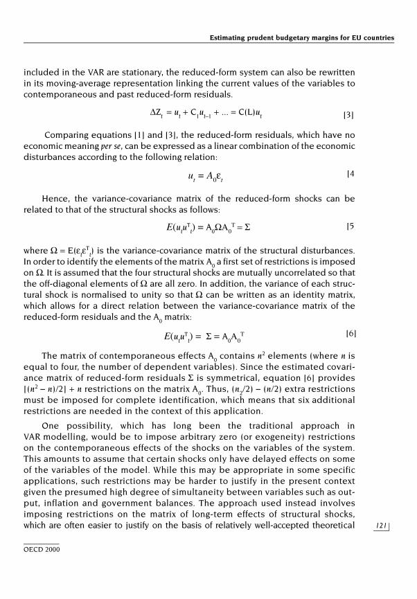
included in the VAR are stationary, the reduced-form system can also be rewrittenin its moving-average representation linking the current values of the variables tocontemporaneous and past reduced-form residuals.

Comparing equations [1] and [3], the reduced-form residuals, which have noeconomic meaning per se, can be expressed as a linear combination of the economicdisturbances according to the following relation:

Hence, the variance-covariance matrix of the reduced-form shocks can berelated to that of the structural shocks as follows:

where Ω = E(εtεT

t) is the variance-covariance matrix of the structural disturbances.In order to identify the elements of the matrix A0 a first set of restrictions is imposedon Ω. It is assumed that the four structural shocks are mutually uncorrelated so thatthe off-diagonal elements of Ω are all zero. In addition, the variance of each struc-tural shock is normalised to unity so that Ω can be written as an identity matrix,which allows for a direct relation between the variance-covariance matrix of thereduced-form residuals and the A0 matrix:

The matrix of contemporaneous effects A0 contains n2 elements (where n isequal to four, the number of dependent variables). Since the estimated covari-ance matrix of reduced-form residuals Σ is symmetrical, equation [6] provides[(n2 – n)/2] + n restrictions on the matrix A0. Thus, (n2/2) – (n/2) extra restrictionsmust be imposed for complete identification, which means that six additionalrestrictions are needed in the context of this application.

One possibility, which has long been the traditional approach inVAR modelling, would be to impose arbitrary zero (or exogeneity) restrictionson the contemporaneous effects of the shocks on the variables of the system.This amounts to assume that certain shocks only have delayed effects on someof the variables of the model. While this may be appropriate in some specificapplications, such restrictions may be harder to justify in the present contextgiven the presumed high degree of simultaneity between variables such as out-put, inflation and government balances. The approach used instead involvesimposing restrictions on the matrix of long-term effects of structural shocks,which are often easier to justify on the basis of relatively well-accepted theoretical

∆Zt = u

t + C

1u

t–1 + ... = C(L)u

t [3]

ut = A0εt [4

E(utuT

t) = A0ΩΑ0Τ = Σ [5]

E(utuT

t) = Σ = A

0Α0

Τ [6]


122

OECD 2000

frameworks. Combining equations [1], [3] and [4], the following relationshipbetween the matrix of long-term effects of structural shocks A(1) and the equiv-alent matrix of reduced-form shocks C(1) is obtained:

Since the matrix C(1) contains known elements (i.e. that are derived fromthe reduced-form estimates), the elements of A0 can be identified by imposingthe six additional restrictions on the matrix of long-run effects A(1). Three of thesix restrictions imposed come from the assumption that neither fiscal policy northe other demand shocks have permanent effects on output, so that the long runoutput level is exclusively determined by supply shocks. Evidently, many the-oretical frameworks would predict that aggregate demand shocks, such as achange in fiscal policy or a shock to private savings, could have some effect onoutput in the long run via relative price changes and their implications for cap-ital accumulation, or if hysteresis effects are present. However, the same mod-els generally predict that the long-run effects of demand-side shocks onproduction are fairly muted relative to the effects of productivity or labour-supplyshocks of comparable magnitudes.

Two additional restrictions are based on the assumptions that real privatedemand shocks and nominal shocks only have temporary effects on the ratio ofgovernment net lending to GDP. While these shocks can have importantshort-run effects on government balances, mainly via the automatic stabilisersmechanism, the presumption is that in the long run, the government net lendingto GDP ratio is unaffected by demand shocks other than those induced by fiscalpolicy. In contrast, no restriction is imposed a priori on the long-run effect of apermanent supply shock on the net lending ratio. The sixth and final restrictionassumes that nominal shocks have a permanent effect on the aggregate pricelevel (or the inflation rate) but leaves all other variables of the systemunchanged in the long run.4

This sort of identifying procedure inevitably entails a certain degree of arbi-trariness and regardless of how strongly one believes in the theoretical underpin-nings of the set of restrictions, the accuracy of the estimates still largely dependson the restrictions’ identifying power which may arguably be relatively weak forsome countries.5

Methodology to derive prudent budgetary margins

Once the VAR model is estimated and the identification of the structuralshocks is achieved, techniques of stochastic simulations are used to assess the risk

A(1) = C(1)A0

[7]


123

OECD 2000

of breaching the 3 per cent deficit level over different time horizons and for giveninitial budget balances.6 Each stochastic simulation generates a hypothetical pathfor the four variables of the model. These paths are based on the random drawing,at each time period, of values for each of the structural disturbances from their esti-mated distribution as well as on their propagation via the estimated lag structureof the VAR model. A different path for the level of the net lending ratio over a ten-year horizon is thus generated in each experiment based on a combination of sup-ply, private demand and nominal shocks whose relative size are determined bytheir estimated variance. As noted above, fiscal policy shocks are turned off in thesimulations in order to capture the pure effects from automatic stabilisation andother induced changes to the budget balance (e.g. interest rate changes,changes to potential output, etc.). It should be stressed, however, that only theunexpected change in fiscal policy is treated as a fiscal shock and turned off in thesimulations. To the extent that fiscal policy has reacted in a systematic and pre-dictable fashion to other economic disturbances in the past, such a fiscal reac-tion function is captured by the lag structure of the VAR system and thereforeplays an active role in the simulations.

For illustrative purposes, Figure 1-A shows three hypothetical simulated pathsfor semi-annual budget balances. For each simulation, the minimum value of thenet lending ratio reached over the relevant time horizon is extracted. In the exam-ple of Figure 1-A, this implies that for an horizon of one year, the net lending ratioscorresponding to points A, B and C would be selected. If the relevant horizon isextended to three years, then points B, D and E are extracted instead. Based on athousand simulations, the minimum values of net lending ratios extracted areranked in ascending order to form a distribution. Such a distribution of minimumnet lending ratios can be drawn for each relevant horizon, up to ten years. As illus-trated in Figure 1-B, the shorter the horizon, the closer to the initial balance will thedistribution be. This is because shocks are assumed to be symmetrically and nor-mally distributed and a short horizon does not allow for significant propagation. Thelonger the time horizon, the higher the probability of a sequence of unfavourableevents hitting the economy and, hence, the further away from the initial level is thedistribution of minimum net lending ratios centred.7 The distribution of budget bal-ances also tends to get wider and flatter as the time horizon increases as shown inFigure 1-B.

Once a distribution over the 1 000 minimum net lending levels is obtained fora specific time horizon, the government net lending ratios associated with differentlevels of cumulated probabilities can be derived. To do so, each distribution is slicedinto percentiles corresponding to different levels of probabilities. For instance, thevalue ranked in the 100th position in the distribution of a thousand observations (orthe 10th percentile) can be interpreted as the minimum net lending ratio that maybe reached with a 90 per cent confidence level.


124

OECD 2000

01 2 3

B

A

C

D

E

05 10

Figure 1-A. Three hypothetical simulated paths for the budget balance

Figure 1-B Hypothetical distributions of minimum budget balance levels

Netlendingratio

Years

Source: Authors.

Distributionof minimumlevels of netlendingratios

Years

01 2 3

B

A

C

D

E

05 10



Netlendingratio

Years

Source: Authors.


Years

01 2 3

B

A

C

D

E

05 10



Netlendingratio

Years

Source: Authors.


Years

01 2 3

B

A

C

D

E

05 10



Netlendingratio

Years

Source: Authors.


Years

01 2 3

B

A

C

D

E

05 10



Netlendingratio

Years

Source: Authors.


Years


125

OECD 2000

CHOICE OF VARIABLES AND MAIN RESULTS FROM THE VAR ESTIMATES

The methodology described in the above section is applied to 11 of the15 EU countries, including eight members of the Euro-area (Germany, France, Italy,Austria, Belgium, Finland, the Netherlands and Spain) and three non-members(the United Kingdom, Denmark and Sweden).8 For each country, a four-variableVAR model is estimated using semi-annual data generally spanning from the early1960s to most recently available observations (generally 1996 or 1997).9 In eachcase, real output (qt) is GDP in volume terms, and the government net lendingratio (nlgqt) is measured as a ratio of government net lending on a national accountsbasis to nominal GDP. Inflation (∆pt) is either the GDP or consumption deflator.Finally, different variables are used across countries to measure net private sectorlending.

The choice for the latter is based on the following National Accounts flow identity:

where S and I are private-sector savings and investment, G and T are public-sectorspending and revenues and X and M are exports and imports of goods and services(including also transfers, interest payments, etc.). The accounting identity [8] sim-ply reflects that in an open economy the excess of private savings over investmentis used to either finance a public-sector deficit or to generate an external accountsurplus. Re-writing [8] in ratios of nominal GDP, and expressing the public-sectorbudget balance as net lending yields:

where nlpq is the ratio of net private savings to nominal GDP, cbq is the current balanceas a ratio of nominal GDP, and nlgq is public net lending as a ratio of nominal GDP.

Based on the identity [9], the variable used in the VAR to capture real pri-vate-sector demand shocks is generally either the private net lending ratio (nlpqt) orthe current account as a per cent of nominal GDP (cbqt). However, in some cases, thegross saving ratio of households (savqt) or real private consumption (cpvt) are used inorder to obtain a longer sample period or better empirical results. As mentionedabove, one additional restriction in choosing the real private demand variable isthat any subset of variables in the VAR-system should not be co-integrated sincethis would violate the assumptions of uncorrelated shocks as well as the long-termrestrictions imposed on the system.

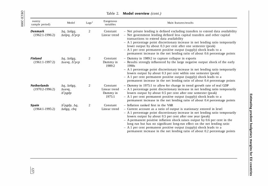
The set of variables chosen for each country is shown in column 2 of Table 2.10

Since the VAR equations must be estimated with stationary variables, they are

S – I = (G – T) + (X – M) [8]

nlpq = cbq – nlgq [9]

OE

CD

Eco

no

mic S

tud

ies N

o. 3

0, 2

00

0/I

126

OE

CD

2000

Table 2. Model overview

ountry ExogenousModel Lags1 Main features/results

sample period) variables

Germany ∆q, ∆nlgq, 4 Constant – Inflation rate is stationary: entered in level(1961:1-1997:2) ∆cpv, ∆pgdp – A 1 per cent point discretionary increase in net lending ratio temporarily

lowers output by about 1 per cent after three semesters (peak)– A permanent output (supply) shock has no significant long-run effect on

the net lending ratio

France ∆q, ∆nlgq, 2 Constant – A 1 per cent point discretionary increase in net lending ratio temporarily(1972:1-1997:2) ∆nlpq, ∆2pcp lowers output by about 0.25 per cent after one semester (peak)

– A 1 per cent permanent positive output (supply) shock leads to apermanent increase in the net lending ratio of about 0.5 percentage points

Italy ∆q, ∆nlgq, 4 Constant – Current account as a ratio of output is stationary: entered in level(1961:1-1996:2) ∆cbq, ∆2pcp Linear trend – A 1 percentage point discretionary increase in net lending ratio temporarily

lowers output by about 0.5 per cent after two years (peak)– A 1 per cent permanent positive output (supply) shock leads to a

permanent increase in the net lending ratio of about 0.4 percentage points

United Kingdom ∆q, ∆nlgq, 4 Constant – Net private lending ratio stationary: entered in level(1965:2-1996:2) nlpq, ∆2pgdp Linear trend – A 1 percentage point discretionary increase in net lending ratio temporarily

lowers output by about 0.7 per cent after three semesters (peak)– A permanent output (supply) shock has no significant long-run effect on

the net lending ratio

Austria ∆q, ∆nlgq, 3 Constant – Inflation rate is stationary: entered in level(1966:1-1995:2) ∆savq, ∆pgdp Linear trend – A 1 percentage point discretionary increase in net lending ratio temporarily

lowers output by about 0.8 per cent within one semester (peak)– A 1 per cent permanent positive output (supply) shock leads to a


Belgium ∆2pgdp, ∆q, 4 Constant – Net private lending is defined excluding transfers to extend data availability(1963:1-1996:2) ∆nlgq, ∆nlpq Linear trend – Inflation ranked first in the VAR

– A 1 percentage point discretionary increase in net lending ratio temporarilylowers output by about 0.7 per cent after three semesters (peak)

– A permanent positive inflation shock raises output by 1.5 per cent in thelong run but has no significant long-run effect on the net lending ratio

– A 1 per cent permanent positive output (supply) shock has no significantlong-run effect on the net lending ratio

Estim

atin

g p

rud

en

t bu

dg

eta

ry ma

rgin

s for E

U co

un

tries

127

OE

CD

2000

Table 2. Model overview (cont.)



Denmark ∆q, ∆nlgq, 2 Constant – Net private lending is defined excluding transfers to extend data availability(1962:1-1996:2) ∆nlpq, ∆2pcp Linear trend – Net government lending defined less capital transfers and other capital

transactions to extend data availability– A 1 percentage point discretionary increase in net lending ratio temporarily

lower output by about 0.3 per cent after one semester (peak)– A 1 per cent permanent positive output (supply) shock leads to a


Finland ∆q, ∆nlgq, 2 Constant – Dummy in 1989:2 to capture collapse in exports(1961:1-1997:2) ∆savq, ∆2pcp Dummy in – Results strongly influenced by the large negative output shock of the early

1989:2 1990s– A 1 percentage point discretionary increase in net lending ratio temporarily

lowers output by about 0.3 per cent within one semester (peak)– A 1 per cent permanent positive output (supply) shock leads to a


Netherlands ∆q, ∆nlgq, 2 Constant – Dummy in 1975:1 to allow for change in trend growth rate of real GDP(1970:2-1996:2) ∆savq, Linear trend – A 1 percentage point discretionary increase in net lending ratio temporarily

∆2pgdp Dummy in lowers output by about 0.5 per cent after one semester (peak)1975:1 – A 1 per cent permanent positive output (supply) shock leads to a


Spain ∆2pgdp, ∆q, 2 Constant – Inflation ranked first in the VAR(1964:1-1995:2) ∆nlgq, cbq Linear trend – Current account as a ratio of output is stationary: entered in level

– A 1 percentage point discretionary increase in net lending ratio temporarilylowers output by about 0.5 per cent after one year (peak)

– A permanent positive inflation shock raises output by 0.6 per cent in thelong run but has no significant long-run effect on the net lending ratio


OE

CD

Eco

no

mic S

tud

ies N

o. 3

0, 2

00

0/I

128

OE

CD

2000

Table 2. Model overview (cont.)



Sweden ∆2pcp, ∆q, 2 Constant – Net private lending is defined excluding transfers to extend data availability(1962:1-1997:1) ∆nlgq, ∆savq Linear trend – Dummy in 1976:1 to capture shift in behaviour of net lending ratio

Dummy in – Inflation ranked first in the VAR1976:1 – A 1 percentage point discretionary increase in net lending ratio temporarily

lowers output by about 0.3 per cent after one semester (peak)– A 1 per cent permanent positive inflation shock raises output by 0.6 per

cent in the long run and leads to a permanent increase in the net lendingratio of about 0.9 percentage points


. The number of lags has been chosen on the basis of the likehood ratio test (5 per cent critical value) over a span of one to six lags (cf. De Serres and Guay, 1995).


129

OECD 2000

generally included in first-difference form.11 In an economic sense, the inclusion ofnet lending ratios in first differences implies that the model does not rule out thepossibility of ever-increasing debt ratios, which indeed has been a characteristic formost EU-countries during the past 25 years. Likewise, by including inflation in firstdifferences for all countries (except for Germany and Austria where inflation isincluded in levels), the possibility of a permanent increase in the rate of inflation isnot ruled out by assumption. The ranking of the variables in the second columnof Table 2 corresponds to the ranking in the VAR system. In most countries, theranking is consistent with the set of long-run restrictions described in the pre-vious section.12

Since no restrictions are imposed on the short-run effect of the shocks, it ispossible to verify whether the identified shocks behave in a way that is consistentwith economic interpretation. For instance, real output and inflation are expectedto move in opposite directions following a supply shock and in the same directionfollowing a demand shock. Moreover, the fiscal policy shock is expected to move thenet lending ratio and output in opposite directions in the short term – or in other words,a tightening of fiscal policy is expected to temporarily lower the level of output.

The main features of the key impulse responses are reported in the last col-umn of Table 2.13 Regarding first the response of government net lending as a ratioof GDP to each of the four shocks, the main characteristics across countries gener-ally confirm the a priori assumptions:

– The net lending ratio (i.e. the fiscal surplus) increases significantly (at the90 per cent confidence level) in response to a contractionary fiscal shock,both in the short and long term.

– A positive supply shock raises the net lending ratio in all countries in theshort term except for Germany, where output improves more than the fiscal bal-ance, leading to a lower ratio. Long-run effects are significant in seven countries:France, Italy, Denmark, Finland, the Netherlands, Spain and Sweden. Thelong-run effect of supply shocks on the net lending ratio is one of the mainfactors driving the outcome of the stochastic simulations.

– The net lending ratio responds positively, but not always significantly, to apositive inflationary shock (exceptions are the United Kingdom and Spain).It responds mostly negatively to a negative real private demand shock, butagain not always in a significant way. In Germany and Sweden, however, pos-itive (negative) real private demand shocks deteriorate (improve) the netlending ratio in the short term, with the effect being significant only in thelatter country. For Germany this is due to the fact that nominal GDPincreases more than government net lending, thus giving rise to a decreas-ing net lending ratio, while for Sweden the model suggest that outputimproves initially in the face of a domestic savings shock. This reaction could


130

OECD 2000

be due to favourable terms of trade effects and/or interest rate crowding in.Long-run effects from monetary shocks and real private demand shocks onthe government’s net lending ratio are ruled out by assumption.

Positive supply shocks raise output significantly in both the short and the longterm. Contractionary fiscal shocks lowers output in the short run14 in all countries,although typically not in a significant way. In all cases, a change in the stance of fiscalpolicy towards consolidation thus leads to a temporary decline in activity (andvice versa) with an elasticity that varies from 0.25 to about 1 per cent. The responseof inflation (price level in the case of Germany and Austria) to supply shocks andfiscal shocks show the expected signs for most countries: a positive supply shock(raises output and) lowers inflation in the short term, and a contractionary fiscalshock lowers (output and) inflation.15 These effects, however, are not significant inmost countries. Finally, for most countries there is a clear tendency for private sav-ings to decrease in the event of a restrictive fiscal shock. To an extent that differsacross countries, this result suggests the presence of crowding-in effects and/orsome degree of income smoothing or partially Ricardian behaviour in the privatesector.

RESULTS OF THE STOCHASTIC SIMULATIONS

The results of the simulations for each country are shown in Figure 2 for differ-ent time horizons and levels of confidence. The budgetary requirements to avoidbreaking the 3 per cent ceiling rises in the desired level of confidence and the timehorizon considered, since over longer time horizons the probability of a series ofadverse events hitting the economies increases. For Germany, for example, thesimulation results suggest that if the government was to aim for a cyclically-adjusteddeficit of 1 per cent of GDP, the actual deficit would, with a 90 per cent likelihood,remain within the 3 per cent limit over a horizon of three years without a need toadjust fiscal policy in a pro-cyclical fashion. This horizon would be extended to tenyears if Germany instead opted for a cyclically-adjusted balanced budget.

Another way to interpret the result is (as can be seen from Figure 2) that thelikelihood of remaining within the 3 per cent threshold for a cyclically-adjusted def-icit of one per cent of GDP would drop from 90 per cent to only 50 per cent if thetime horizon considered by policy makers extends from three to ten years. Theresults also reveal that most countries face relatively similar trade-offs betweenbudget targets and levels of confidence. Cyclically-adjusted budgetary positionsaround balance, or even small deficits, would thus provide most countries with a 90 percent likelihood of keeping the deficit within the 3 per cent margin over a three tofive-year horizon without having to resort to discretionary pro-cyclical fiscal tightening(Figure 3). However, for the three countries outside the euro-area (the United Kingdom,


131

OECD 2000

50 60 70 80 10090Level of confidence (%)





43210-1-2-3-4

43210

-1-2-3-4

543210-1-2

-4-3

543210

-1-2

-4-3

3

2

1

0

-1

-2

-3

-4

3

2

1

0

-1

-2

-3

-4

43210

-1-2

-4-3

43210-1-2

-4-3

Figure 2. Cyclically adjusted balance required to meetthe 3 per cent deficit criterion with different levels of confidence

1 year

Source: Authors’ calculations.

Balance in per cent of GDP Balance in per cent of GDP

Germany France

1.51.00.5

0-0.5-1.0-1.5-2.0

-3.0-2.5

Balance in per cent of GDP

Spain


Italy United Kingdom

1.51.00.50-0.5-1.0-1.5-2.0

-3.0-2.5

3 years 5 years 10 years






43210-1-2-3-4

43210

-1-2-3-4

543210-1-2

-4-3

543210

-1-2

-4-3

3

2

1

0

-1

-2

-3

-4

3

2

1

0

-1

-2

-3

-4

43210

-1-2

-4-3

43210-1-2

-4-3


1 year



Germany France

1.51.00.5

0-0.5-1.0-1.5-2.0

-3.0-2.5


Spain



1.51.00.50-0.5-1.0-1.5-2.0

-3.0-2.5







43210-1-2-3-4

43210

-1-2-3-4

543210-1-2

-4-3

543210

-1-2

-4-3

3

2

1

0

-1

-2

-3

-4

3

2

1

0

-1

-2

-3

-4

43210

-1-2

-4-3

43210-1-2

-4-3


1 year



Germany France

1.51.00.5

0-0.5-1.0-1.5-2.0

-3.0-2.5


Spain



1.51.00.50-0.5-1.0-1.5-2.0

-3.0-2.5







43210-1-2-3-4

43210

-1-2-3-4

543210-1-2

-4-3

543210

-1-2

-4-3

3

2

1

0

-1

-2

-3

-4

3

2

1

0

-1

-2

-3

-4

43210

-1-2

-4-3

43210-1-2

-4-3


1 year



Germany France

1.51.00.5

0-0.5-1.0-1.5-2.0

-3.0-2.5


Spain



1.51.00.50-0.5-1.0-1.5-2.0

-3.0-2.5







43210-1-2-3-4

43210

-1-2-3-4

543210-1-2

-4-3

543210

-1-2

-4-3

3

2

1

0

-1

-2

-3

-4

3

2

1

0

-1

-2

-3

-4

43210

-1-2

-4-3

43210-1-2

-4-3


1 year



Germany France

1.51.00.5

0-0.5-1.0-1.5-2.0

-3.0-2.5


Spain



1.51.00.50-0.5-1.0-1.5-2.0

-3.0-2.5



132

OECD 2000



50 60 70 80 10090Level of confidence (%) Level of confidence (%)

1.00.50-0.5-1.0-1.5-2.0-2.5-3.0

1.00.5

0-0.5-1.0-1.5-2.0-2.5-3.0


1.00.5

0-0.5-1.0-1.5-2.0-2.5

-3.5-3.0

1.00.50-0.5-1.0-1.5-2.0-2.5

-3.5-3.0

8

6

4

2

0

-2

-4

8

6

4

2

0

-2

-4

6543210

-1

-4-3-2

6543210-1

-4

-2-3

1.51.00.5

0-0.5-1.0-1.5

-3.5-3.0

-2.0-2.5

1.51.00.50-0.5-1.0-1.5

-3.5-3.0

-2.0-2.5

1210

86420

-2-4

121086420-2-4

50 60 70 80 10090

50 60 70 80 10090

Figure 2. Cyclically adjusted balance required to meetthe 3 per cent deficit criterion with different levels of confidence (cont.)

1 year



Austria Belgium


Denmark Finland



Netherlands Sweden




1.00.50-0.5-1.0-1.5-2.0-2.5-3.0

1.00.5

0-0.5-1.0-1.5-2.0-2.5-3.0


1.00.5

0-0.5-1.0-1.5-2.0-2.5

-3.5-3.0

1.00.50-0.5-1.0-1.5-2.0-2.5

-3.5-3.0

8

6

4

2

0

-2

-4

8

6

4

2

0

-2

-4

6543210

-1

-4-3-2

6543210-1

-4

-2-3

1.51.00.5

0-0.5-1.0-1.5

-3.5-3.0

-2.0-2.5

1.51.00.50-0.5-1.0-1.5

-3.5-3.0

-2.0-2.5

1210

86420

-2-4

121086420-2-4

50 60 70 80 10090

50 60 70 80 10090


1 year



Austria Belgium


Denmark Finland



Netherlands Sweden




1.00.50-0.5-1.0-1.5-2.0-2.5-3.0

1.00.5

0-0.5-1.0-1.5-2.0-2.5-3.0


1.00.5

0-0.5-1.0-1.5-2.0-2.5

-3.5-3.0

1.00.50-0.5-1.0-1.5-2.0-2.5

-3.5-3.0

8

6

4

2

0

-2

-4

8

6

4

2

0

-2

-4

6543210

-1

-4-3-2

6543210-1

-4

-2-3

1.51.00.5

0-0.5-1.0-1.5

-3.5-3.0

-2.0-2.5

1.51.00.50-0.5-1.0-1.5

-3.5-3.0

-2.0-2.5

1210

86420

-2-4

121086420-2-4

50 60 70 80 10090

50 60 70 80 10090


1 year



Austria Belgium


Denmark Finland



Netherlands Sweden




1.00.50-0.5-1.0-1.5-2.0-2.5-3.0

1.00.5

0-0.5-1.0-1.5-2.0-2.5-3.0


1.00.5

0-0.5-1.0-1.5-2.0-2.5

-3.5-3.0

1.00.50-0.5-1.0-1.5-2.0-2.5

-3.5-3.0

8

6

4

2

0

-2

-4

8

6

4

2

0

-2

-4

6543210

-1

-4-3-2

6543210-1

-4

-2-3

1.51.00.5

0-0.5-1.0-1.5

-3.5-3.0

-2.0-2.5

1.51.00.50-0.5-1.0-1.5

-3.5-3.0

-2.0-2.5

1210

86420

-2-4

121086420-2-4

50 60 70 80 10090

50 60 70 80 10090


1 year



Austria Belgium


Denmark Finland



Netherlands Sweden




1.00.50-0.5-1.0-1.5-2.0-2.5-3.0

1.00.5

0-0.5-1.0-1.5-2.0-2.5-3.0


1.00.5

0-0.5-1.0-1.5-2.0-2.5

-3.5-3.0

1.00.50-0.5-1.0-1.5-2.0-2.5

-3.5-3.0

8

6

4

2

0

-2

-4

8

6

4

2

0

-2

-4

6543210

-1

-4-3-2

6543210-1

-4

-2-3

1.51.00.5

0-0.5-1.0-1.5

-3.5-3.0

-2.0-2.5

1.51.00.50-0.5-1.0-1.5

-3.5-3.0

-2.0-2.5

1210

86420

-2-4

121086420-2-4

50 60 70 80 10090

50 60 70 80 10090


1 year



Austria Belgium


Denmark Finland



Netherlands Sweden


133

OECD 2000

Denmark and Sweden) the requirements are somewhat higher – i.e. surpluses in therange of 0.7 – 2.4 per cent of GDP would be needed over a five years horizon.

The results indicate that the medium-term deficit targets – as set out in theindividual countries’ Stability programmes (for euro-area countries) and Conver-gence programmes (for non-euro countries) that were submitted to the EuropeanCommission in the in the fall of 1998 (Table 3) – appear to be overall prudent, atleast with respect to a three-year horizon. Stated differently, the simulation resultsimply that if governments aim for a cyclically-adjusted deficit (or surplus) corre-sponding to the level specified in their own respective programmes, the actual def-icit will, with a likelihood of close to 90 per cent, remain within the 3 per cent limitover a three-year horizon. However, over a horizon extended to five years, the like-lihood of not breaching the ceiling drops to around 70-80 per cent for the four larg-est economies and Austria, whereas it remains above the 90 per cent confidencelevel for the rest of the countries (Figure 4).

This suggests that a cyclically-adjusted deficit target of 1-1.5 per cent of GDParound 2002 in Germany, France, Italy and Austria, as well as a balanced budget inthe United Kingdom, might not provide a strong medium-term hedge againstbreaking the 3 per cent limit, though a five-year horizon might appear sufficientlylong to policymakers to steer the deficit in the appropriate direction without unduly

Netherl

andsAustr

ia

Belgium

Spain

Germany

Italy

France

Finlan

d

United Kingdom

Denmark

3

2

1

0

-1

-2

-3

3

2

1

0

-1

-2

-3

Sweden

Figure 3. Cyclically-adjusted government balances required to meetthe 3 per cent of GDP deficit criterion with 90 per cent confidence

over different time horizons

1 year

Per cent of GDP Per cent of GDP


3 years 5 years

Netherl

andsAustr

ia

Belgium

Spain

Germany

Italy

France

Finlan

d

United Kingdom

Denmark

3

2

1

0

-1

-2

-3

3

2

1

0

-1

-2

-3

Sweden



1 year



3 years 5 years

Netherl

andsAustr

ia

Belgium

Spain

Germany

Italy

France

Finlan

d

United Kingdom

Denmark

3

2

1

0

-1

-2

-3

3

2

1

0

-1

-2

-3

Sweden



1 year



3 years 5 years

Netherl

andsAustr

ia

Belgium

Spain

Germany

Italy

France

Finlan

d

United Kingdom

Denmark

3

2

1

0

-1

-2

-3

3

2

1

0

-1

-2

-3

Sweden



1 year



3 years 5 years

Netherl

andsAustr

ia

Belgium

Spain

Germany

Italy

France

Finlan

d

United Kingdom

Denmark

3

2

1

0

-1

-2

-3

3

2

1

0

-1

-2

-3

Sweden



1 year



3 years 5 years

OE

CD

Eco

no

mic S

tud

ies N

o. 3

0, 2

00

0/I

134

OE

CD

2000

Table 3. Official medium-term programmes to comply with the Stability and Growth Pact1

Deficit Debt Deficit target Debt ratio Expenditure ratio Underlying annual GDP growth1998 1998 2002 2002 2002 Projection

As a per cent of GDP2 1999 2000-02

ustria 2.2 64.4 1.4 60.0 48.9 2.8 2.3elgium 1.3 117.5 0.3 106.8 46.2 2.4 2.3inland –1.1 51.9 –2.3 43.2 45.4 4.0 2.6

rance 2.9 58.2 0.8-1.2 57.1-58.3 50.6-51.5 2.4-2.7 2.5-3.0ermany 2.1 61.0 1.0 59.5 45.0 2.0 2.5

reland3 –1.7 59.0 –1.6 43.0 28.1 6.7 6.1taly3 2.6 118.2 1.0 107.0 48.3 2.5 2.9

etherlands 1.3 68.6 1.1 64.5 43.8 2.3 2.3ortugal 2.3 58.0 0.8 53.2 39.8 3.5 3.3pain 1.9 67.4 –0.1 59.3 41.2 3.8 3.3

enmark3 –1.1 59.0 –2.6 49.0 < 48.6 1.7 2.0reece3 2.4 107.8 0.8 99.8 39.3 3.7 4.2weden3 –1.5 74.2 –2.5 58.0 58.0 2.2 2.5nited Kingdom –0.8 47.9 –0.2 42.0 40.1 1.0 2.6

. Submitted to the European Commission in December, 1998.

. Negative numbers denote a surplus.

. Deficit target, debt ratio, expenditure ratio and underlying annual GDP growth projections are for 2001 instead of 2002 and 2000-02, respectively.ource: European Commission and national authorities.


135

OECD 2000

exacerbating the cycle, providing action is taken early enough. On the other hand,more ambitious medium-term targets may be desirable if one considers additionalfactors such as the implications of population ageing on pension and health carecosts.

It should be stressed that the study does not address the question ofexcessive deficits, i.e. to what extent deficits above 3 per cent of GDP willco-exist with severe recessions (fall in real GDP of at least ¾ per cent) or byother means be exempted from the excessive deficit procedure in the ECOFINcouncil. This implies, that the de facto risk of having to undertake pro-cyclical fis-cal tightening during an economic downturn is slightly lower than indicated bythe simulations. This caveat, however, is likely to be of minor importance to thepolicy implications of the simulation results since historically only some 10 percent of the episodes of deficits above 3 per cent of GDP (for EU-15) haveoccurred simultaneously with a drop in real GDP of more than 0.75 per cent (andonly 2-3 per cent have occurred when real GDP was falling by more than 2 percent). Another reason is that deficits sometimes lag behind real activity suchthat the provisions of the Stability and Growth Pact concerning severe economicdownturns may not apply in the same years as the deficit exceeds the 3 per cent

100

90

80

70

60

50

100

90

80

70

60

50

Per cent Per cent

1. As stated in the medium-term stability or convergence programmes (December 1998).2. The programme for France presents two different scenarios with a projected deficit in 2002 of respectively 0.8

and 1.2 per cent of GDP. The latter is used as reference here.Source: Authors’ calculations.

Figure 4. Likelihood that the official budget target1 will allowcompliance with the deficit limit

3 years

Germany

France

2

Austria

Italy

United Kingdom

Netherl

ands

Sweden

Belgium

SpainFin

land

Denmark

5 years

100

90

80

70

60

50

100

90

80

70

60

50

Per cent Per cent




3 years

Germany

France

2

Austria

Italy

United Kingdom

Netherl

ands

Sweden

Belgium

SpainFin

land

Denmark

5 years

100

90

80

70

60

50

100

90

80

70

60

50

Per cent Per cent




3 years

Germany

France

2

Austria

Italy

United Kingdom

Netherl

ands

Sweden

Belgium

SpainFin

land

Denmark

5 years

100

90

80

70

60

50

100

90

80

70

60

50

Per cent Per cent




3 years

Germany

France

2

Austria

Italy

United Kingdom

Netherl

ands

Sweden

Belgium

SpainFin

land

Denmark

5 years

100

90

80

70

60

50

100

90

80

70

60

50

Per cent Per cent




3 years

Germany

France

2

Austria

Italy

United Kingdom

Netherl

ands

Sweden

Belgium

SpainFin

land

Denmark

5 years


136

OECD 2000

limit. Finally, the results are obtained using semi-annual data. Since the Stabil-ity and Growth Pact is concerned solely with annual budget outcomes, thederived levels of confidence could be biased (even though the raw semi-annualdata used are annualised). However, sensitivity analysis using the averages oftwo consecutive semi-annual observations to convert the results into calendaryears does not display significant differences to the results obtained by semi-annual data (typically the cyclically adjusted net lending ratio for any givenlevel of confidence and time horizon would deviate by a maximum of 0.1-0.2 percentage point of GDP).

It should also be emphasised that the estimated budgetary requirementsdo not, or only partly, capture more recent changes to political and budgetaryframeworks as well as to economic structures, and that particular historical epi-sodes may be dominating the results for some countries. The most notableexamples are Finland and Sweden, both of which have been experiencingextreme changes in the budget balances since 1990. These episodes imply thatthe VAR model identifies some excessive shocks for Finland and Sweden, whichin turn lead to results for prudent budgetary margins that are somewhat higherthan what would be relevant when considering the current economic environ-ment and policy framework in the two countries. In order to better capture likelyfuture shocks for these two economies, it was thus chosen to base the results onan average of shocks experienced by the four major EU-economies rather thanpast shocks in the countries themselves.16

The simulation results should be considered policy-relevant mainly fortime horizons no longer than five years since beyond that horizon the cumulativeeffects of non-linearities in the economic variables (which may not be properly cap-tured by the model) could blur the results.17 Moreover, planning horizons of up tofive years are quite common for fiscal policy.

The differences in the results across countries can largely be explained bythree factors:

– The variance of the change in the deficit: higher variance implies higher bud-getary requirements;

– The importance of fiscal policy shocks – relative to the other three types ofshocks – in explaining movements in the deficit: the more important is therole of fiscal shocks, the lower the budgetary requirement (because fiscalshocks are turned off in the simulations);

– The quality of the VAR model, i.e. how much of the volatility in thefour variables is captured by the lag structure of the model and how muchremains in the residuals. Intuitively, it may not matter much whether theunconditional variance of the variables is captured ultimately by the vari-ance of the residuals or by the lag structure. However, it may have some


137

OECD 2000

influence on the final results given that one of the shocks (i.e. the fiscalshock) is turned off in the simulations.

Government net lending-to-GDP ratios for the eleven countries are shown inFigure 5. The least volatile deficits over the 1960-97 period have been found inGermany, France, Austria and the Netherlands, whereas deficits in Italy, Finland andSweden have had the largest volatility. Based on movements in deficit levels, onemight expect to find more stringent budget requirements in the latter countries to pro-vide for an adequately prudent budgetary margin. However, for purposes of automaticstabilisation, it is important to distinguish between the cyclical change in the deficit andits long-term drift. A large variance of the deficit level reflects, in most cases, the pres-ence of a unit root and should therefore not necessarily be interpreted as a meaningfulindication of the sensitivity of the budget balance to business cycles developments.Indeed, since the deficit is included in the VAR in first differences, it is the variance ofthe change in the deficit level – rather than the variance of the level – that has a deter-mining influence on the outcome (in the sense that the higher the variance,ceteris paribus, the more stringent the budget requirements will be).

The cases of the United Kingdom and Italy are illustrative in this respect. Italyhas had much higher volatility in the government net lending-to-GDP ratio thanthe United Kingdom, but Italy’s deficit has shown a long and relatively smoothdownward trend followed by a long and smooth correction, whereas theUK deficit ratio has been dominated by two major cycles (Figure 5). The impli-cation is that volatility of the first difference of the deficit ratio has been lowerin Italy than in the United Kingdom. This would tend to imply a lower budgetrequirement in Italy than in the United Kingdom. Figure 6 shows a relativelyclose link between the variance of the first difference of the deficit ratio and thebudgetary requirement (here illustrated by the case with 90 per cent confi-dence and a three-year horizon). The volatility of the change in the deficit indi-cates that countries like Austria, Belgium, the Netherlands and Spain would facerelatively low budgetary requirements, whereas Finland and, in particular,Sweden18 would need significantly better budget positions to achieve the samesafety margin. Germany, France, the United Kingdom, Italy and Denmark are inintermediate positions.

The relative importance of fiscal policy shocks in explaining the movementsin the deficit also has an important influence on the cross-country differences.If a large part of the unpredicted movement in the deficit is accounted for byfiscal-policy-induced shocks, then the budgetary requirement would be relativelylow given that such shocks are turned off in the simulations. This partly explains thesomewhat less stringent safety margin needed in Germany relative to France andItaly (over 1-3 per cent horizons) despite a comparable variance in the change inthe deficit ratio. On the opposite side, the very stringent requirements obtained for


138

OECD 2000

7

0

-141961:S1 65:S1 69:S1 73:S1 1997:S177:S1 81:S1 85:S1 89:S1 93:S1

7

0

-14

7

0

-7

-14

7

0

-7

-141961:S1 65:S1 69:S1 73:S1 1997:S177:S1 81:S1 85:S1 89:S1 93:S1

7

0

-7

-141961:S1 65:S1 69:S1 73:S1 1997:S177:S1 81:S1 85:S1 89:S1 93:S1

7

0

-7

-14

7

0

-7

-14

7

0

-7

-141961:S1 65:S1 69:S1 73:S1 1997:S177:S1 81:S1 85:S1 89:S1 93:S1

7

0

-7

-14

7

0

-7

-141961:S1 65:S1 69:S1 73:S1 1997:S177:S1 81:S1 85:S1 89:S1 93:S1

-7 -7

Figure 5. Government net lendingin per cent of GDP

Source: OECD, Economic Outlook 63 databank.

Per cent of GDP

Germany France



Per cent of GDP

Spain

Per cent of GDP

7

0

-141961:S1 65:S1 69:S1 73:S1 1997:S177:S1 81:S1 85:S1 89:S1 93:S1

7

0

-14

7

0

-7

-14

7

0

-7

-141961:S1 65:S1 69:S1 73:S1 1997:S177:S1 81:S1 85:S1 89:S1 93:S1

7

0

-7

-141961:S1 65:S1 69:S1 73:S1 1997:S177:S1 81:S1 85:S1 89:S1 93:S1

7

0

-7

-14

7

0

-7

-14

7

0

-7

-141961:S1 65:S1 69:S1 73:S1 1997:S177:S1 81:S1 85:S1 89:S1 93:S1

7

0

-7

-14

7

0

-7

-141961:S1 65:S1 69:S1 73:S1 1997:S177:S1 81:S1 85:S1 89:S1 93:S1

-7 -7



Per cent of GDP

Germany France



Per cent of GDP

Spain

Per cent of GDP

7

0

-141961:S1 65:S1 69:S1 73:S1 1997:S177:S1 81:S1 85:S1 89:S1 93:S1

7

0

-14

7

0

-7

-14

7

0

-7

-141961:S1 65:S1 69:S1 73:S1 1997:S177:S1 81:S1 85:S1 89:S1 93:S1

7

0

-7

-141961:S1 65:S1 69:S1 73:S1 1997:S177:S1 81:S1 85:S1 89:S1 93:S1

7

0

-7

-14

7

0

-7

-14

7

0

-7

-141961:S1 65:S1 69:S1 73:S1 1997:S177:S1 81:S1 85:S1 89:S1 93:S1

7

0

-7

-14

7

0

-7

-141961:S1 65:S1 69:S1 73:S1 1997:S177:S1 81:S1 85:S1 89:S1 93:S1

-7 -7



Per cent of GDP

Germany France



Per cent of GDP

Spain

Per cent of GDP

7

0

-141961:S1 65:S1 69:S1 73:S1 1997:S177:S1 81:S1 85:S1 89:S1 93:S1

7

0

-14

7

0

-7

-14

7

0

-7

-141961:S1 65:S1 69:S1 73:S1 1997:S177:S1 81:S1 85:S1 89:S1 93:S1

7

0

-7

-141961:S1 65:S1 69:S1 73:S1 1997:S177:S1 81:S1 85:S1 89:S1 93:S1

7

0

-7

-14

7

0

-7

-14

7

0

-7

-141961:S1 65:S1 69:S1 73:S1 1997:S177:S1 81:S1 85:S1 89:S1 93:S1

7

0

-7

-14

7

0

-7

-141961:S1 65:S1 69:S1 73:S1 1997:S177:S1 81:S1 85:S1 89:S1 93:S1

-7 -7



Per cent of GDP

Germany France



Per cent of GDP

Spain

Per cent of GDP

7

0

-141961:S1 65:S1 69:S1 73:S1 1997:S177:S1 81:S1 85:S1 89:S1 93:S1

7

0

-14

7

0

-7

-14

7

0

-7

-141961:S1 65:S1 69:S1 73:S1 1997:S177:S1 81:S1 85:S1 89:S1 93:S1

7

0

-7

-141961:S1 65:S1 69:S1 73:S1 1997:S177:S1 81:S1 85:S1 89:S1 93:S1

7

0

-7

-14

7

0

-7

-14

7

0

-7

-141961:S1 65:S1 69:S1 73:S1 1997:S177:S1 81:S1 85:S1 89:S1 93:S1

7

0

-7

-14

7

0

-7

-141961:S1 65:S1 69:S1 73:S1 1997:S177:S1 81:S1 85:S1 89:S1 93:S1

-7 -7



Per cent of GDP

Germany France



Per cent of GDP

Spain

Per cent of GDP


139

OECD 2000

7

0

-141961:S1 65:S1 69:S1 73:S1 1997:S177:S1 81:S1 85:S1 89:S1 93:S1

7

-7

-14

7

-7

-14

7

-7

-141961:S1 65:S1 69:S1 73:S1 1997:S177:S1 81:S1 85:S1 89:S1 93:S1

1961:S1 65:S1 69:S1 73:S1 1997:S177:S1 81:S1 85:S1 89:S1 93:S1 1961:S1 65:S1 69:S1 73:S1 1997:S177:S1 81:S1 85:S1 89:S1 93:S1


-7

0 0 0

7

0

-14

7

-7

-14

7

-7

-14

7

-7

-14

-7

0 0 0

7

0

-14

7

-7

-14

7

-7

-14

7

-7

-14

-7

0 0 0

Figure 5. Government net lendingin per cent of GDP (cont.)


Per cent of GDP

Austria Belgium


Denmark Finland

Per cent of GDP


Netherlands Sweden

7

0

-141961:S1 65:S1 69:S1 73:S1 1997:S177:S1 81:S1 85:S1 89:S1 93:S1

7

-7

-14

7

-7

-14

7

-7

-141961:S1 65:S1 69:S1 73:S1 1997:S177:S1 81:S1 85:S1 89:S1 93:S1



-7

0 0 0

7

0

-14

7

-7

-14

7

-7

-14

7

-7

-14

-7

0 0 0

7

0

-14

7

-7

-14

7

-7

-14

7

-7

-14

-7

0 0 0



Per cent of GDP

Austria Belgium


Denmark Finland

Per cent of GDP


Netherlands Sweden

7

0

-141961:S1 65:S1 69:S1 73:S1 1997:S177:S1 81:S1 85:S1 89:S1 93:S1

7

-7

-14

7

-7

-14

7

-7

-141961:S1 65:S1 69:S1 73:S1 1997:S177:S1 81:S1 85:S1 89:S1 93:S1



-7

0 0 0

7

0

-14

7

-7

-14

7

-7

-14

7

-7

-14

-7

0 0 0

7

0

-14

7

-7

-14

7

-7

-14

7

-7

-14

-7

0 0 0



Per cent of GDP

Austria Belgium


Denmark Finland

Per cent of GDP


Netherlands Sweden

7

0

-141961:S1 65:S1 69:S1 73:S1 1997:S177:S1 81:S1 85:S1 89:S1 93:S1

7

-7

-14

7

-7

-14

7

-7

-141961:S1 65:S1 69:S1 73:S1 1997:S177:S1 81:S1 85:S1 89:S1 93:S1



-7

0 0 0

7

0

-14

7

-7

-14

7

-7

-14

7

-7

-14

-7

0 0 0

7

0

-14

7

-7

-14

7

-7

-14

7

-7

-14

-7

0 0 0



Per cent of GDP

Austria Belgium


Denmark Finland

Per cent of GDP


Netherlands Sweden

7

0

-141961:S1 65:S1 69:S1 73:S1 1997:S177:S1 81:S1 85:S1 89:S1 93:S1

7

-7

-14

7

-7

-14

7

-7

-141961:S1 65:S1 69:S1 73:S1 1997:S177:S1 81:S1 85:S1 89:S1 93:S1



-7

0 0 0

7

0

-14

7

-7

-14

7

-7

-14

7

-7

-14

-7

0 0 0

7

0

-14

7

-7

-14

7

-7

-14

7

-7

-14

-7

0 0 0



Per cent of GDP

Austria Belgium


Denmark Finland

Per cent of GDP


Netherlands Sweden


140

OECD 2000

Denmark and Sweden are partly attributable to the strong influence exerted bysupply shocks on the deficit in the long run.

Finally, variations in the quality of the four estimated equations of theVAR model can also explain some of the cross-country differences in the results.Poorly estimated VAR equations mean that a larger portion of the fluctuations in thevariables are accounted for by the model’s residuals. In turn, this implies that largershocks are drawn during the simulations. The effects are not unambiguous, how-ever, since a poorly estimated model may display a lower propagation of the shock– and hence a lower budgetary requirement.

SENSITIVITY ANALYSIS

In order to asses the implication for the results of leaving out the fiscal shock,the simulations have also been carried out when including all four shocks(Figure 7). It turns out, as expected, that the inclusion of the fiscal shock raises thebudgetary requirements (additional volatility requires higher margins). However,the relative ranking of countries remains fairly unchanged – and the stricter require-

2.5

2.0

1.5

1.0

0.5

0

-0.5

-1.0

-1.5

-2.0

2.5

2.0

1.5

1.0

0.5

0

-0.5

-1.0

-1.5

-2.0

Figure 6. Cyclically-adjusted budget balance requirementsand volatility in deficits

Budgetary requirement (90 per cent confidence over 3 years)



Netherl

andsSpain

Austria

Belgium Ita

lyFra

nce

Germany

Finlan

d

Denmark

United Kingdom

Sweden

Variance of first difference of deficit radio

2.5

2.0

1.5

1.0

0.5

0

-0.5

-1.0

-1.5

-2.0

2.5

2.0

1.5

1.0

0.5

0

-0.5

-1.0

-1.5

-2.0





Netherl

andsSpain

Austria

Belgium Ita

lyFra

nce

Germany

Finlan

d

Denmark

United Kingdom

Sweden


2.5

2.0

1.5

1.0

0.5

0

-0.5

-1.0

-1.5

-2.0

2.5

2.0

1.5

1.0

0.5

0

-0.5

-1.0

-1.5

-2.0





Netherl

andsSpain

Austria

Belgium Ita

lyFra

nce

Germany

Finlan

d

Denmark

United Kingdom

Sweden


2.5

2.0

1.5

1.0

0.5

0

-0.5

-1.0

-1.5

-2.0

2.5

2.0

1.5

1.0

0.5

0

-0.5

-1.0

-1.5

-2.0





Netherl

andsSpain

Austria

Belgium Ita

lyFra

nce

Germany

Finlan

d

Denmark

United Kingdom

Sweden


2.5

2.0

1.5

1.0

0.5

0

-0.5

-1.0

-1.5

-2.0

2.5

2.0

1.5

1.0

0.5

0

-0.5

-1.0

-1.5

-2.0





Netherl

andsSpain

Austria

Belgium Ita

lyFra

nce

Germany

Finlan

d

Denmark

United Kingdom

Sweden



141

OECD 2000

ments for Finland, the United Kingdom, Denmark, and Sweden are maintained. Theinclusion of the fiscal shock changes the results most significantly in France and thethree Nordic countries. This could capture a genuine relatively large effect from fis-cal policy decisions on past budgetary dynamics, but it could also be a result ofthe model allocating too much weight to fiscal shocks. In any case, the robustnessof the country ranking to the inclusion of all four shocks implies that the exactinterpretation of the shocks is not decisive for the relative requirements for thecountries – i.e. even if the model does not accurately capture what is “true”demand (fiscal, real private and monetary) and supply shocks the relative positionof countries remains nearly unaltered.

Simulations have also been carried out in order to assess the sensitivity of theresults to changes in the variable measuring real private demand. Table 4 showsthat uniformly using net private lending (in first differences) only implies mar-ginal changes for the countries where other variables have been used in thebaseline model – i.e. the budgetary requirement changes by less than 0.2 per centof GDP in all cases (except for Finland). Simulations have also been carried out totest the impact of ranking inflation last – instead of first – for Spain, Belgium andSweden. Once again, the budgetary requirements change only slightly, i.e. less than0.4 per cent of GDP for a five years horizon and 90 per cent confidence. Finally, the

Austria Ita

ly

Netherl

ands

Belgium

Spain

Germany

France

United Kingdom

Finlan

d

Denmark

Sweden

5

4

3

2

1

0

-2

-1

5

4

3

2

1

0

-2

-1

Figure 7. Cyclically adjusted government balances required to meetthe 3 per cent of GDP deficit criterion with 90 per cent confidence

over a 3 year horizon

Excluding fiscal shock



Including fiscal shock

Austria Ita

ly

Netherl

ands

Belgium

Spain

Germany

France

United Kingdom

Finlan

d

Denmark

Sweden

5

4

3

2

1

0

-2

-1

5

4

3

2

1

0

-2

-1







Austria Ita

ly

Netherl

ands

Belgium

Spain

Germany

France

United Kingdom

Finlan

d

Denmark

Sweden

5

4

3

2

1

0

-2

-1

5

4

3

2

1

0

-2

-1







Austria Ita

ly

Netherl

ands

Belgium

Spain

Germany

France

United Kingdom

Finlan

d

Denmark

Sweden

5

4

3

2

1

0

-2

-1

5

4

3

2

1

0

-2

-1







Austria Ita

ly

Netherl

ands

Belgium

Spain

Germany

France

United Kingdom

Finlan

d

Denmark

Sweden

5

4

3

2

1

0

-2

-1

5

4

3

2

1

0

-2

-1








142

OECD 2000

sensitivity of the results to a change in the lag length has been examined and foundto be fairly low, although with the three Nordic countries exhibiting a non-negligiblesensitivity (Table 5). Taken together these sensitivity results imply that the budgetary

Table 4. Sensitivity of results to a change in the variable measuring real privatedemand

Three year horizon Five year horizon(90 per cent confidence) (90 per cent confidence)

Base model With D1NLPQ Base model With D1NLPQ

Germany (D1CPV) –0.85 –0.74 –0.54 –0.43France (D1NLPQ) –1.02 – –0.42 –Italy (CBQ) –1.03 –0.91 –0.43 –0.40United Kingdom (NLPQ) 0.04 – 0.68 –Spain (CBQ) –1.35 –1.43 –0.85 –0.88Austria (D1SRATIO) –1.25 –1.30 –0.92 –0.89Belgium (D1NLPQ) –1.18 – –0.88 –Netherlands (D1SRATIO) –1.55 –1.52 –1.15 –1.13Finland (D1SRATIO) –0.68 0.28 0.14 1.48Denmark (D1NLPQ) –0.16 – 0.77 –Sweden (D1SRATIO) 1.06 0.90 2.37 2.16

Note: The variable measuring real private demand in the base model is indicated in the parenthesis.A ‘‘–’’ implies that NLQP or D1NLQP is used as the base model for the country concerned.


Table 5. Sensitivity of results to a change in the lag length of the VAR model

Three-year horizon Five-year horizon(90 per cent confidence) (90 per cent confidence)

Optimal lag Optimal lag Optimal lag Optimal lagOptimal lag Optimal lag

minus one plus one minus one plus one

Germany –0.25 –0.85 –0.75 0.13 –0.54 –0.35France –1.04 –1.02 –1.12 –0.30 –0.42 –0.58Italy –0.80 –1.03 –1.36 0.10 –0.43 –0.83United Kingdom 0.34 0.04 –0.20 1.20 0.68 0.42Spain –0.97 –1.35 –1.24 –0.33 –0.85 –0.45Austria –1.37 –1.25 –1.50 –1.00 –0.92 –1.22Belgium –1.13 –1.18 –1.04 –0.73 –0.88 –0.57Netherlands –1.40 –1.55 –1.73 –0.82 –1.15 –1.40Finland –0.06 –0.68 –0.81 1.24 0.14 –0.05Denmark –0.38 –0.16 1.00 0.80 0.77 2.98Sweden 2.41 1.06 2.01 5.00 2.37 3.95



143

OECD 2000

requirements found by using different country-specific models are fairly robustcompared with applying exactly the same model for all countries (i.e. same vari-ables, ordering and lag length).

CONCLUSION

A two-step methodology has been used to estimate prudent budgetarymargins, i.e. cyclically adjusted balances that would allow automatic fiscal stabi-lisers to fully operate over the business cycle while preventing the general gov-ernment deficit to breach the limit of 3 per cent of GDP set under the Stabilityand Growth Pact. A structural VAR model has been estimated for 11 EU coun-tries, capturing the effects on the deficit of economic shocks that have histori-cally prevailed in each country. Based on the estimated distributions of theseshocks, stochastic simulations have then been performed to build up probabil-ities of breaching the 3 per cent ceiling in the future. During each simulation, fis-cal policy was assumed to be unchanged in order to purely capture themovements in the deficit stemming from automatic stabilisation and othersources not originating from fiscal impulses (i.e. movements due to supplyshocks, real private demand shocks and monetary shocks). Under this method-ology, budget targets become more stringent as longer-term horizons are considered,because the probability of a sequence of unfavourable events hitting an economyincreases over time.

The simulation results suggest that, for the majority of countries, if govern-ments were to aim for a cyclically-adjusted budget deficit between 1.0 and 1.5 percent of GDP, the actual deficit would, with a 90 per cent likelihood, remain withinthe 3 per cent limit over a three-year horizon, without the need to adjust fiscalpolicy in a pro-cyclical fashion. This horizon would be extended to five yearsand above if governments opted for a “close-to-balance” budget rule, definedas a cyclically-adjusted deficit between zero and 1 per cent of GDP. Given thatsuch a horizon encompasses the average length of a business cycle, theseresults largely endorse the recommendations of the SGP and the conclusionsreached by Buti et al. (1998). For Finland, the United Kingdom and Denmark (inascending order), moderate (cyclically-adjusted) surpluses would be needed tominimise the risks of breaching the 3 per cent limit over a five year horizon,whereas the requirement for Sweden is a more substantial surplus to achieve tosame level of confidence.

The results indicate that the medium-term deficit targets – as set out in theindividual countries’ Stability programmes (for euro-area countries) and Conver-gence programmes (for non-euro countries) – submitted to the European Councilappear to be overall prudent, at least with respect to a three-year horizon. Over


144

OECD 2000

longer horizons, however, the results suggest that for the four largest economiesand Austria, the deficit targets might not provide as strong a hedge against breach-ing the 3 per cent of GDP deficit limit. The results also suggest that cross-countrydifferences in medium-term budget targets are well justified in light of the pastrecord on fluctuations in net lending ratios.


145

OECD 2000

NOTES

1. Such estimates of elasticities are, of course, subject to uncertainty, temporal instability, and inparticular, they could be affected by EMU participation. In any case, the OECD Secretariat esti-mates are similar to those used by the IMF and the European Commission.

2. Taking the variation in output gaps into consideration, the IMF shows how a structural budgetaryposition between balance and a deficit of 1 per cent of GDP would accommodate full automaticstabilisation within the 3 per cent limit with 95 per cent confidence (assuming output gaps in allthe euro-area countries are drawn from the same normal distribution).

3. For a review of topics in structural VAR econometrics, see Amisano and Giannini (1997).

4. This set of restrictions assumes that all the variables in the system should be integrated of thesame order but should not be co-integrated.

5. As described below, the set of restrictions has been slightly modified for a few countries in orderto obtain impulse responses that seemed more compatible with economic priors.

6. Interpreted as the cyclically-adjusted level of government net lending.

7. Likewise, the distribution of maximum values would be centred around increasingly highersurpluses.

8. There are no government accounts for Luxembourg, while it has not been possible to obtainwell-specified models for Portugal and Greece, partly due to problems with the governmentaccount data for these countries. Ireland has been excluded since government accounts dataonly goes back to 1977, implying potential problems with too few degrees of freedom.

9. Semi-annual data was chosen in order to get sufficient degrees of freedom for the models. Oneproblem with using semi-annual data for fiscal analysis is that budget balances follow yearly patternsand semi-annual data may thus be misleading in some cases. Moreover the data for the other vari-ables – especially for some of the smaller countries – sometimes exhibit an apparently excessiveerratic behaviour from one semester to another.

10. All the data are taken from the OECD Outlook Data Bank and are measured on a National Accountsbasis.

11. Standard unit root tests have been used to determine the order of integration.

12. Exceptions are Spain, Belgium and Sweden where the change in inflation is ranked first in theVAR rather than last. In those cases, permanent inflation shocks (which are interpreted as mon-etary shocks) can have permanent effects on output and the net lending ratio. The re-orderingis justified in those cases by the finding that under the baseline ranking, the disturbances interpretedas supply shocks in fact behaved as demand shocks (i.e. a positive shock raises both output and infla-tion). This can be interpreted as evidence of hysteresis. It turns out that the ranking of inflation hasonly marginal effects for the final outcomes of the stochastic simulations for these three countries(i.e. the results are invariant to whether inflation is ranked first or last in the system).


146

OECD 2000

13. Given space limitations, impulse response figures are not shown in this paper but are availableupon request from the authors or can be found in the working paper version (Dalsgaard andde Serres, 1999, website www.oecd.org/eco/eco).

14. Fiscal policy is restricted to have temporary effects on the level of output.15. Exceptions to this are Belgium, Spain, the United Kingdom and Sweden where inflation rises at

impact and then starts falling after two to four semesters.

16. Based on the country-specific shocks instead of the average of the major-four country shocksthe budget requirement over a five-years horizon and 90 per cent confidence would be 3.7 percent of GDP for Sweden (instead of 2.4) and 1.4 per cent of GDP for Finland (instead of 0.1).

17. This is particularly true for countries where the aggregate supply shock is found to have a per-manent effect on the budget balance (in addition to the fiscal shock itself which is turned off dur-ing simulations). In such cases, the variance of the simulated budget balance tends to increasecontinuously with the length of the horizon.

18. Besides the volatility of the deficit, several studies have found a somewhat higher sensitivity ofthe budget to cyclical movements in output for Sweden than for other EU countries (cf. Table 1).


147

OECD 2000

BIBLIOGRAPHY

AMISANO, G. and C. GIANNINI (1997), Topics in Structural VAR Econometrics, Second Edition,Springer-Verlag, Heidelberg.

BECKER, T. (1997), “An investigation of Ricardian equivalence in a common trends model”, Journalof Monetary Economics, Vol. 39, pp. 405-431.

BLANCHARD, O. and D. QUAH (1989), “The dynamic effect of aggregate demand and supply dis-turbances”, American Economic Review, Vol. 79, No. 4.

BRUNEAU, C. and O. DE BANDT (1997), “Fiscal policy in the transition to monetary union: Astructural VAR model”, conference paper.

BUTI, M., D. FRANCO and H. ONGENA (1997), “Budgetary policies during recessions – retrospectiveapplication of the Stability and Growth Pact to the post-war period”, European Commission,Economic Papers, No. 121.

BUTI, M., D. FRANCO and H. ONGENA (1998), “Fiscal discipline and flexibility in EMU: the imple-mentation of the Stability and Growth Pact”, Oxford Review of Economic Policy, Vol. 14, No. 3.

DALSGAARD, T. and A. DE SERRES (1999), “Estimating prudent budgetary margins for 11 EU countries:a simulated SVAR model approach”, Working Paper No. 216, OECD Economics Department, Paris.

DE SERRES, A. and A. GUAY (1995), “The selection of the truncation lag in structural VARs (orVECMs) with long-run restrictions”, Working Paper, 95-9, Bank of Canada, Ottawa.

INTERNATIONAL MONETARY FUND (1998a), “Economic policy challenges facing the euro area andthe external implications of the Euro”, Background Annex for the World Economic Outlook, Autumn.

INTERNATIONAL MONETARY FUND (1998b), “France: selected issues. Fiscal stabilizers underEMU”, IMF Staff Country Report, No. 98/132, December.

KOREN, S. and A. STIASSNY (1998), “Tax and spend, or spend and tax? An international study”,Journal of Policy Modelling, Vol. 20, No. 2.

LUTKEPOHL, H. (1990), “Asymptotic distribution of impulse response functions and forecasterror variance decomposition of vector autoregressive models” Review of Economic and Statistics,Vol. 72, No. 1.

OECD (1997), Economic Outlook 62, Paris, December.

OECD (1998), Economic Outlook 64, Paris, December.

ROODENBURG, H., R. JANSSEN and H. TER RELE (1998), “Assessing a safety margin for the fiscaldeficit vis-à-vis the EMU ceiling”, De Economist, Vol. 146, No. 3.

estimating prudent budgetary margins for … · 115 oecd 2000 oecd economic studies no. 30, 2000/i...

Documents