ESTIMATING PUMPING TIME AND GROUND-WATER

WITHDRAWALS USING ENERGY-CONSUMPTION DATA

By R. Theodore Hurr and David W. Litke

U.S. GEOLOGICAL SURVEY

Water-Resources Investigations Report 89-4107

Prepared in cooperation with the

COLORADO DEPARTMENT OF NATURAL RESOURCES,

DIVISION OF WATER RESOURCES,

OFFICE OF THE STATE ENGINEER

Denver, Colorado 1989

DEPARTMENT OF THE INTERIOR

MANUEL LUJAN, JR., Secretary

U.S. GEOLOGICAL SURVEY

Dallas L. Peck, Director

For additional information write to:

District Chief U.S. Geological Survey Box 25046, Mail Stop 415 Federal Center Denver, CO 80225-0046

Copies of this report can be purchased from:

U.S. Geological SurveyBooks and Open-File Reports SectionBox 25425Federal CenterDenver, CO 80225-0425

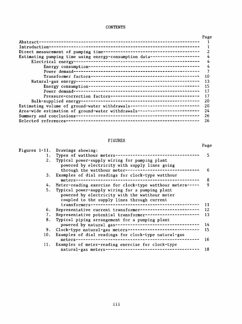
CONTENTS

PageAbstract - -- -- - - --- ------------- _______ _______ ________ iIntroduction------------- ------------------- _______ ________________ \Direct measurement of pumping time----------- ------- ------- ________ 2Estimating pumping time using energy-consumption data-- ---------------- 4

Electrical energy--------------------------------------------------- 4Energy consumption----------------- ----- _________________ 4Power demand---------- ____________________________--__------- 7Transformer factors-------------------------------------------- 10

Natural-gas energy-------------------------------------------------- 13Energy consumption--------------------------------------------- 15Power demand------------------------------------------ ------- 17Pressure-correction factors------------------------------------ 17

Bulk-supplied energy---------- ------------------ _______--_--- - 20Estimating volume of ground-water withdrawals----------- --------------- 20Area-wide estimation of ground-water withdrawals---------------- ------- 24Summary and conclusions------------------------------ ----------------- 26Selected references-------------------------- ---- --- ------ _______ 26

FIGURESPage

Figures 1-11. Drawings showing:1. Types of watthour meters---------------------------------- 52. Typical power-supply wiring for pumping plant

powered by electricity with supply lines goingthrough the watthour meter------------------------------ 6

3. Examples of dial readings for clock-type watthourmeters- _________ _____________ _____________________ g

4. Meter-reading exercise for clock-type watthour meters--- 95. Typical power-supply wiring for a pumping plant

powered by electricity with the watthour meter coupled to the supply lines through current transformers------------------------------------------ 11

6. Representative current transformer------------------------ 127. Representative potential transformer--- ----- ---------- 138. Typical piping arrangement for a pumping plant

powered by natural gas---------------------------------- 149. Clock-type natural-gas meters----------------------------- 15

10. Examples of dial readings for clock-type natural-gasmeters------ --_-_-__________-_--_ _________________ 15

11. Examples of meter-reading exercise for clock-typenatural-gas meters-------------------------------------- 18

111

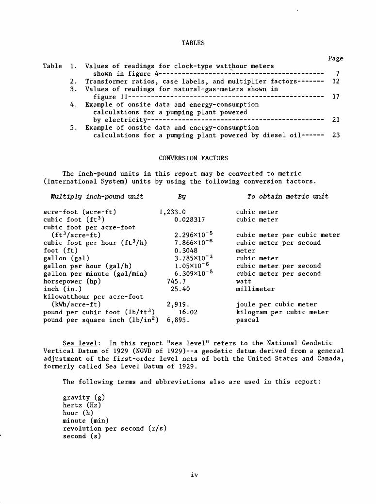
TABLES

Table 1. Values of readings for clock-type watthour metersshown in figure 4------------------------------ ------

2. Transformer ratios, case labels, and multiplier factors--3. Values of readings for natural-gas-meters shown in

figure ll----------------------------- ---------------4. Example of onsite data and energy-consumption

calculations for a pumping plant powered by electricity------------ ----------- _______-- __.

5. Example of onsite data and energy-consumptioncalculations for a pumping plant powered by diesel oil-

Page

712

17

21

23

CONVERSION FACTORS

The inch-pound units in this report may be converted to metric (International System) units by using the following conversion factors.

Multiply inch-pound unit

acre-foot (acre-ft)cubic foot (ft 3 )cubic foot per acre-foot

(ft 3 /acre-ft)cubic foot per hour (ft 3 /h) foot (ft) gallon (gal) gallon per hour (gal/h) gallon per minute (gal/min) horsepower (hp) inch (in.) kilowatthour per acre-foot

(kWh/acre-ft)pound per cubic foot (lb/ft 3 ) pound per square inch (lb/in2 )

By

1,233.00.028317

2.296xiO~ 57.866xiO~ 60.30483.785X10' 31.05X10" 66.309X10

745.7 25.40

2,919.16.02

6,895.

-5

To obtain metric unit

cubic meter cubic meter

cubic meter per cubic metercubic meter per secondmetercubic metercubic meter per secondcubic meter per secondwattmillimeter

joule per cubic meter kilogram per cubic meter pascal

Sea level: In this report "sea level" refers to the National Geodetic Vertical Datum of 1929 (NGVD of 1929)--a geodetic datum derived from a general adjustment of the first-order level nets of both the United States and Canada, formerly called Sea Level Datum of 1929.

The following terms and abbreviations also are used in this report:

gravity (g)hertz (Hz)hour (h)minute (min)revolution per second (r/s)second (s)

IV

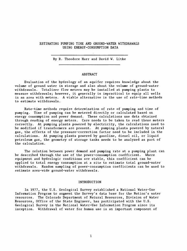
ESTIMATING PUMPING TIME AND GROUND-WATER WITHDRAWALS USING ENERGY-CONSUMPTION DATA

By R. Theodore Hurr and David W. Litke

ABSTRACT

Evaluation of the hydrology of an aquifer requires knowledge about the volume of ground water in storage and also about the volume of ground-water withdrawals. Totalizer flow meters may be installed at pumping plants to measure withdrawals; however, it generally is impractical to equip all wells in an area with meters. A viable alternative is the use of rate-time methods to estimate withdrawals.

Rate-time methods require determination of rate of pumping and time of pumping. Time of pumping can be metered directly or calculated based on energy consumption and power demand. These calculations use data obtained through reading of energy meters. Care needs to be taken to read these meters correctly. At pumping plants powered by electricity, the calculations need to be modified if transformers are present. At pumping plants powered by natural gas, the effects of the pressure-correction factor need to be included in the calculations. At pumping plants powered by gasoline, diesel oil, or liquid petroleum gas, the geometry of storage tanks needs to be analyzed as part of the calculation.

The relation between power demand and pumping rate at a pumping plant can be described through the use of the power-consumption coefficient. Where equipment and hydrologic conditions are stable, this coefficient can be applied to total energy consumption at a site to estimate total ground-water withdrawals. Random sampling of power-consumption coefficients can be used to estimate area-wide ground-water withdrawals.

INTRODUCTION

In 1977, the U.S. Geological Survey established a National Water-Use Information Program to augment the Survey's data base for the Nation's water resources. The Colorado Department of Natural Resources, Division of Water Resources, Office of the State Engineer, has participated with the U.S. Geological Survey in the National Water-Use Information Program since its inception. Withdrawal of water for human use is an important component of

the hydrologic budget; in particular, evaluation of the hydrology of an aqui­ fer requires knowledge about the volume of ground water in storage and also about the volume of ground-water withdrawals.

Several methods may be used to determine the volume of ground-water withdrawals some indirect and others direct (Baker, 1979). Indirect methods commonly are used to estimate withdrawals by applying an assumed use rate; for instance, irrigation withdrawals may be indirectly estimated by applying a theoretical crop water-use requirement to a known acreage under cultivation. Direct methods are those in which the withdrawal volume is either metered or is calculated by multiplying a pumping rate by a cumulative pumping time (rate-time methods). Direct volume metering by inline totalizer meters or flow recorders is amply discussed in the literature (Addison, 1941; Rohwer, 1942; Linford, 1961; Kilpatrick, 1965; U.S. Bureau of Reclamation, 1974; Hayward, 1979). This report focuses on rate-time methods.

Rate-time methods are based on the relation that the volume of water pumped is equal to the average pumping rate multiplied by the pumping time. This relation is mathematically expressed as:

V = Q x t , (1)

where V = volume of water pumped,Q = average pumping rate, in volume per time, and t = pumping time.

Therefore, to calculate the volume of water that is pumped, a repre­ sentative pumping rate needs to be measured and pumping time needs to be determined. Many methods of measuring pumping rate are described in the literature (Rohwer, 1942; U.S. Bureau of Reclamation, 1974; Marella and Singleton, 1988). However, methods to determine pumping time are less well documented. The purpose of this report is to describe how to derive pumping- time information, primarily through the use of energy-consumption data. Further, this report describes methods for "rating" pumping plants; that is, pumping-rate and energy-consumption information are combined into a single factor that then can be used to estimate ground-water withdrawals. Methods applicable to the various common types of pumping plants and fuels are pre­ sented. Although the methods described here are presented in the context of determination of ground-water withdrawals, they also are applicable to pumping plants where surface water is withdrawn.

DIRECT MEASUREMENT OF PUMPING TIME

Direct measurement of pumping time can be manual or automatic. Manual measurement requires that the well owner or pump operator keep a written, chronological log of pump operations by recording each time the pump is turned on and each time the pump is turned off. The total pumping time then is deter­ mined by summing the individual periods of pumping.

Automatic measurement of pumping time can be made by a recorder that tracks the periods of pumping, which are then summed in the same manner as in the manual method, or by a clock that records elapsed time and only operates when the pump is operating. Frequently, internal-combustion powerplants are equipped with hour meters that record hours of operation in much the same way that odometers on cars record miles of operation. The number of hours of operation in a given period then is the hour-meter reading at the end of the period minus the hour-meter reading at the beginning of the period. If the final reading is smaller than the initial reading, the numbers in the meter register probably have "turned over," so that the turnover reading needs to be added to the final reading before the initial reading is subtracted. For example:

Initial reading: 856.9 hoursFinal reading: 035.7 hoursTurnover reading: 1,000.0 hours

(035.7 + 1,000.0) - 856.9 = 178.8 hours of operation.

Use of an odometer-type hour meter to determine pumping time may provide unsatisfactory results, because the meters are not always reliable. Hour meters may be exposed to the weather and constant vibrations from the pump, and they also are susceptible to electric surges and lightning strikes. A backup clock or operations log, therefore, is desirable.

A second type of hour meter is the vibration-time totalizer (VTT), which was developed by the U.S. Geological Survey. This battery-powered sensor attaches to pump equipment and senses vibrations to determine pumping time. The sensor needs to be attached at a place where sufficient vibrations occur when the pump is on; the VTT can sense vibrations over a broad frequency range (20 to 2,000 Hz) when the duration is longer than 0.5 s and the sustained acceleration is 0.5 g or more. The sensor uses a piezoelectric element to convert vibration energy into an electrical signal. Time of operation is accumulated and displayed through an eight-digit, liquid-crystal display. Although this device is relatively new (developed in 1987), initial indica­ tions are that it is reliable and accurate (George Pyper, U.S. Geological Survey, oral commun., 1988).

A third type of hour meter is the inductive-time totalizer (ITT). This device, which is commercially available, senses current movement in the supply line that powers electrical pumps (and, hence, cannot be used for natural-gas- powered pumps). The meter is attached to the supply line by simply wrapping two wires around the supply line without removing the insulation. The sensor is virtually a transformer that generates a small current through induction whenever electricity is passing through the supply line to the electric pump motor. This device also is reliable and accurate (Richard Marella, U.S. Geological Survey, oral commun., 1988).

ESTIMATING PUMPING TIME USING ENERGY-CONSUMPTION DATA

Pumping time can be calculated from energy-consumption data, as follows:

= energy power '

where t = pumping time,energy = quantity of electricity or fuel consumed, and power = rate of electricity or fuel consumption.

Electricity and natural gas are the most common types of energy used to power pumps. These types of energy usually are supplied by utility companies that install meters at each site. Utility companies may provide annual energy-consumption information for aggregated areas but may not provide more detailed site-specific information. For most studies it is necessary to read meters to develop needed energy-consumption data. Less commonly used fuels, such as gasoline, diesel oil, and liquid petroleum gas, are purchased in bulk. Fuel-consumption records for bulk fuels commonly are kept by the user. The following sections describe methods for deriving pumping-time information from energy-consumption data.

Electrical Energy

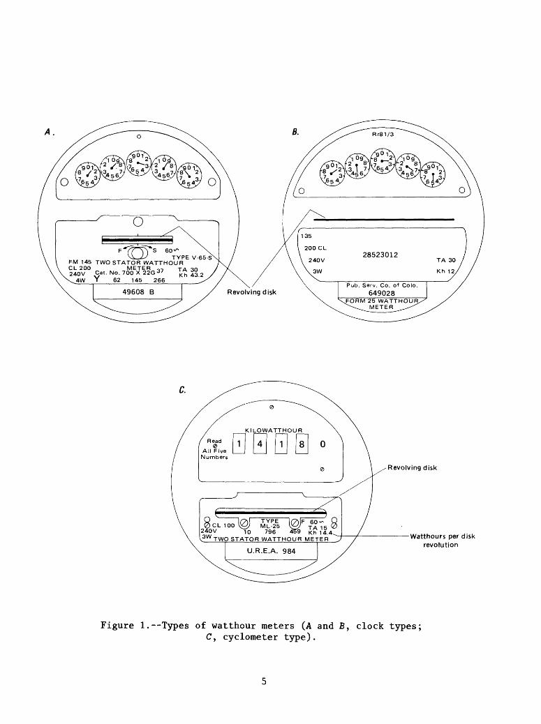
Electricity meters, called watthour meters, record the quantity of elec­ tricity (energy) consumed at a pumping plant. There are two basic types of meters: clock and cyclometer (fig. 1). Most commonly, these meters are wired directly into the circuit that provides electricity to the pump (fig. 2). The unit of electrical-energy consumption is the kilowatthour (kWh).

Both types of watthour meters contain a disk that revolves as electricity passes through the meter. By timing the rate at which this disk revolves, the rate of electrical-energy consumption (power) can be determined. The rate of electrical-energy consumption is measured in kilowatts (kW).

Pumping time can be calculated using equation 2 which, for electric meters, becomes:

. ,. ^ energy (kilowatthours) ro x t (hours) = ft/ v n ._ ? - . (3) power (kilowatts)

To apply this equation, energy consumption and power demand need to be deter­ mined at each pumping plant.

Energy Consumption

Electrical-energy consumption is determined by reading watthour meters. The clock-type watthour meter usually consists of five circular dials and

A.

C.

TYPE ML-25

10 796 459 Khl.4 TWOSTATORWATTHOUR METER

Revolving disk

Watthours per disk revolution

Figure 1.--Types of watthour meters (A and B, clock types;C y cyclometer type).

Pow

er

pole

with

th

ree p

hase

tra

nsf

orm

ers

Mete

r p

ole

Ele

ctric

moto

r

Un

de

rgro

un

d

conduit

Figu

re 2.

--Ty

pica

l power-supply wiring

for

a pumping

plant

powered

by el

ectr

icit

y wi

thsu

pply

li

nes

goin

g th

roug

h the

watt

hour

meter.

pointers arranged side by side (figs. 1A and B). The pointers are driven by a series of interconnecting gears. The pointer on the right (units position) ^drives the next pointer to the left (tens position), which in turn drives the next pointer to the left, and so on. Because of the gearing arrangement, each pointer rotates in a direction counter to the others. The five-pointer meter will indicate a number as large as 99,999 kWh. On some clock-type meters, a "xlO" multiplier is imprinted on the faceplate that enables the meter to indi­ cate a number as large as 999,990 kWh.

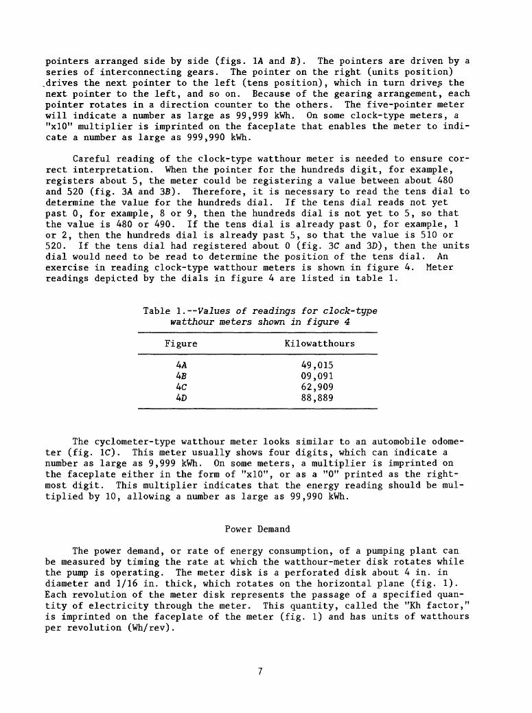
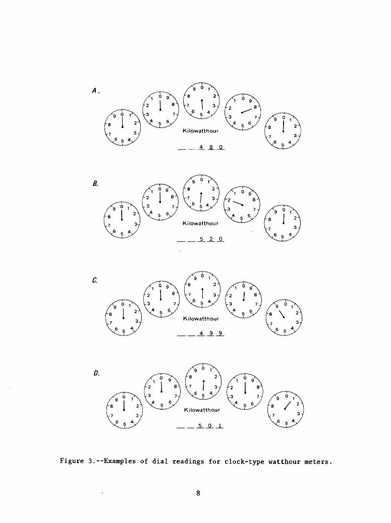
Careful reading of the clock-type watthour meter is needed to ensure cor­ rect interpretation. When the pointer for the hundreds digit, for example, registers about 5, the meter could be registering a value between about 480 and 520 (fig. 3A and 3B). Therefore, it is necessary to read the tens dial to determine the value for the hundreds dial. If the tens dial reads not yet past 0, for example, 8 or 9, then the hundreds dial is not yet to 5, so that the value is 480 or 490. If the tens dial is already past 0, for example, 1 or 2, then the hundreds dial is already past 5, so that the value is 510 or 520. If the tens dial had registered about 0 (fig. 3C and 3D), then the units dial would need to be read to determine the position of the tens dial. An exercise in reading clock-type watthour meters is shown in figure 4. Meter readings depicted by the dials in figure 4 are listed in table 1.

Table 1. Values of readings for clock-type watthour meters shown in figure 4

Figure Kilowatthours

4A 49,0154B 09,0914C 62,9094D 88,889

The cyclometer-type watthour meter looks similar to an automobile odome­ ter (fig. 1C). This meter usually shows four digits, which can indicate a number as large as 9,999 kWh. On some meters, a multiplier is imprinted on the faceplate either in the form of "xlO", or as a "0" printed as the right­ most digit. This multiplier indicates that the energy reading should be mul­ tiplied by 10, allowing a number as large as 99,990 kWh.

Power Demand

The power demand, or rate of energy consumption, of a pumping plant can be measured by timing the rate at which the watthour-meter disk rotates while the pump is operating. The meter disk is a perforated disk about 4 in. in diameter and 1/16 in. thick, which rotates on the horizontal plane (fig. 1). Each revolution of the meter disk represents the passage of a specified quan­ tity of electricity through the meter. This quantity, called the "Kh factor," is imprinted on the faceplate of the meter (fig. 1) and has units of watthours per revolution (Wh/rev).

A.

B.

C.

Kilowatthour

499

D.

Kilowatthour

___5__Q_ JL

Figure 3.--Examples of dial readings for clock-type watthour meters

A.

B.

c.

D.

Figure 4.--Meter-reading exercise for clock-type watthour meters

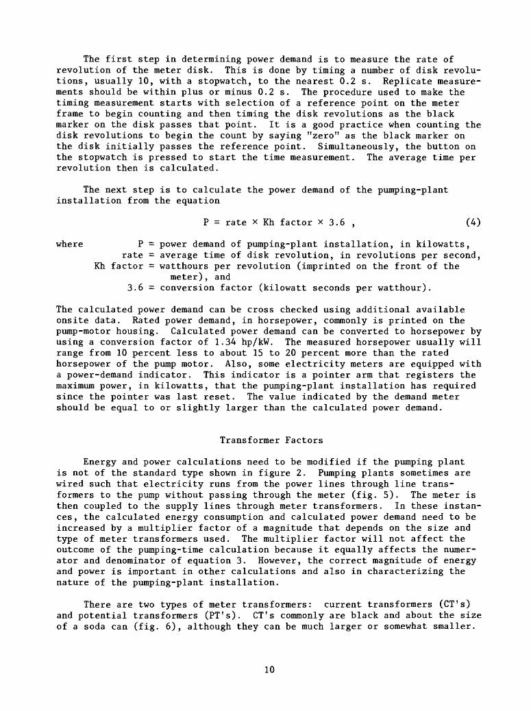
The first step in determining power demand is to measure the rate of revolution of the meter disk. This is done by timing a number of disk revolu­ tions, usually 10, with a stopwatch, to the nearest 0.2 s. Replicate measure­ ments should be within plus or minus 0.2 s. The procedure used to make the timing measurement starts with selection of a reference point on the meter frame to begin counting and then timing the disk revolutions as the black marker on the disk passes that point. It is a good practice when counting the disk revolutions to begin the count by saying "zero" as the black marker on the disk initially passes the reference point. Simultaneously, the button on the stopwatch is pressed to start the time measurement. The average time per revolution then is calculated.

The next step is to calculate the power demand of the pumping-plant installation from the equation

P = rate x Kh factor x 3.6 , (4)

where P = power demand of pumping-plant installation, in kilowatts,rate = average time of disk revolution, in revolutions per second,

Kh factor = watthours per revolution (imprinted on the front of themeter), and

3.6 = conversion factor (kilowatt seconds per watthour).

The calculated power demand can be cross checked using additional available onsite data. Rated power demand, in horsepower, commonly is printed on the pump-motor housing. Calculated power demand can be converted to horsepower by using a conversion factor of 1.34 hp/kW. The measured horsepower usually will range from 10 percent less to about 15 to 20 percent more than the rated horsepower of the pump motor. Also, some electricity meters are equipped with a power-demand indicator. This indicator is a pointer arm that registers the maximum power, in kilowatts, that the pumping-plant installation has required since the pointer was last reset. The value indicated by the demand meter should be equal to or slightly larger than the calculated power demand.

Transformer Factors

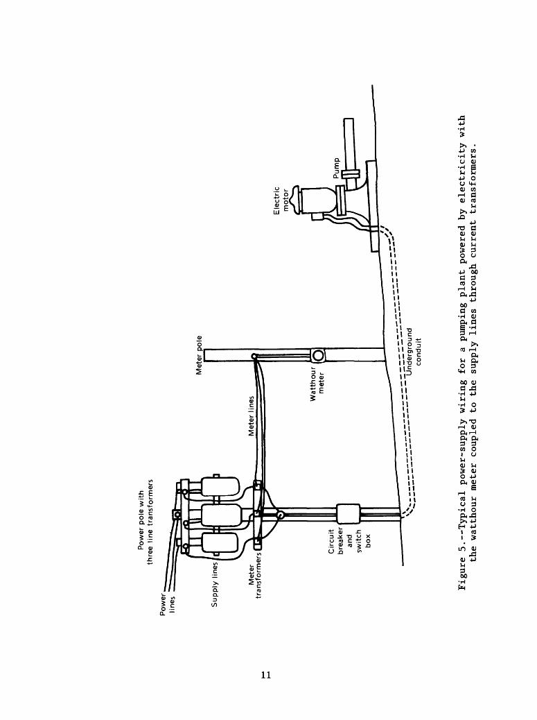
Energy and power calculations need to be modified if the pumping plant is not of the standard type shown in figure 2. Pumping plants sometimes are wired such that electricity runs from the power lines through line trans­ formers to the pump without passing through the meter (fig. 5). The meter is then coupled to the supply lines through meter transformers. In these instan­ ces , the calculated energy consumption and calculated power demand need to be increased by a multiplier factor of a magnitude that depends on the size and type of meter transformers used. The multiplier factor will not affect the outcome of the pumping-time calculation because it equally affects the numer­ ator and denominator of equation 3. However, the correct magnitude of energy and power is important in other calculations and also in characterizing the nature of the pumping-plant installation.

There are two types of meter transformers: current transformers (CT's) and potential transformers (PT's). CT's commonly are black and about the size of a soda can (fig. 6), although they can be much larger or somewhat smaller.

10

Pow

er

po

le w

ith

th

ree lin

e t

ran

sfo

rme

rs

Me

ter

pole

Ele

ctric

moto

r

Underg

round

conduit

Figu

re 5. Typical power-supply w

iring

for

a pu

mpin

g pl

ant

powe

red

by el

ectr

icit

y wi

th

the

watt

hour

me

ter

coup

led

to th

e su

pply

lines

thro

ugh

current

transformers.

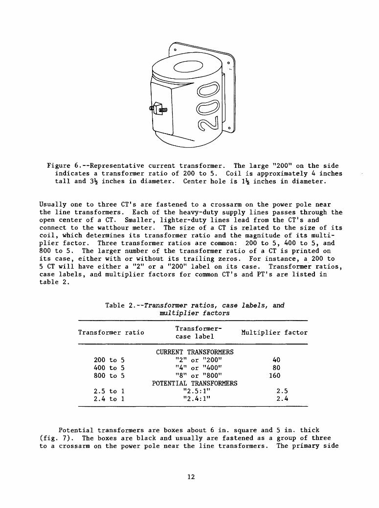
Figure 6.--Representative current transformer. The large "200" on the side indicates a transformer ratio of 200 to 5. Coil is approximately 4 inches tall and 3^ inches in diameter. Center hole is \\ inches in diameter.

Usually one to three CT's are fastened to a crossarm on the power pole near the line transformers. Each of the heavy-duty supply lines passes through the open center of a CT. Smaller, lighter-duty lines lead from the CT's and connect to the watthour meter. The size of a CT is related to the size of its coil, which determines its transformer ratio and the magnitude of its multi­ plier factor. Three transformer ratios are common: 200 to 5, 400 to 5, and 800 to 5. The larger number of the transformer ratio of a CT is printed on its case, either with or without its trailing zeros. For instance, a 200 to 5 CT will have either a "2" or a "200" label on its case. Transformer ratios, case labels, and multiplier factors for common CT's and PT's are listed in table 2.

Table 2. Transformer ratios, case labels, and multiplier factors

Transformer ratioTransformer- case label

Multiplier factor

200 to 5 400 to 5 800 to 5

2.5 to 1 2.4 to 1

CURRENT TRANSFORMERS "2" or "200" "4" or "400" "8" or "800"

POTENTIAL TRANSFORMERS "2.5:1" "2.4:1"

4080160

2.5 2.4

Potential transformers are boxes about 6 in. square and 5 in. thick(fig. 7). The boxes are black and usually are fastened as a group of threeto a crossarm on the power pole near the line transformers. The primary side

12

Figure 7.--Representative potential transformer. The number on the front of the transformer indicates a transformer ratio of 2.5 to 1. The transformer is about 6 inches square and 5 inches thick.

of the PT's connects to the supply line leading from the line transformer to the switch box. The secondary side of the PT's connects to the watthour meter. The transformer ratio for PT's used for electrically powered pumping plants is 2.5 to 1, with a multiplier factor of 2.5 (table 2), although some older PT's may have a ratio of 2.4:1 and a factor of 2.4. The ratio is indi­ cated on the plate that is fastened on the front of the PT.

CT's may be used singly, or in combination with PT's, but PT's are not used alone. If both are used, calculated energy and power need to be multi­ plied by the CT factor and the PT factor. For example, in the presence of CT's and PT's, equation 4 becomes

P = rate x Kh factor x 3.6 x CT factor x PT factor (5)

Natural-Gas Energy

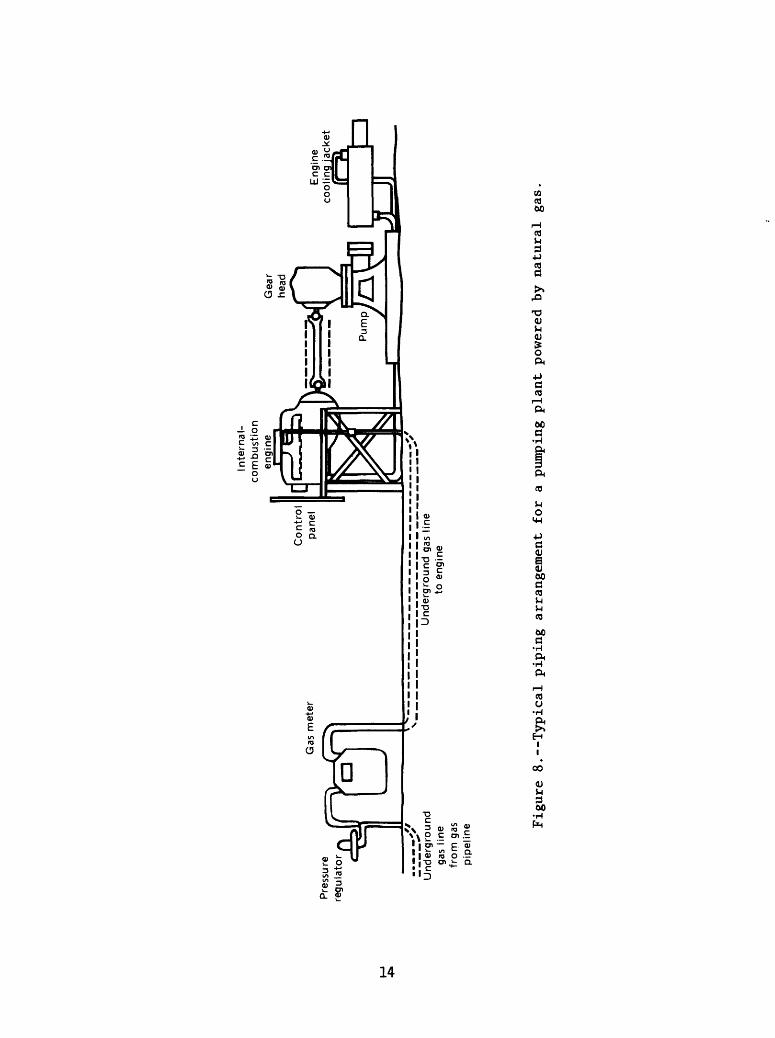
Natural gas can be burned in an internal combustion engine that in turn powers a mechanical pump. A typical pumping plant powered by natural gas is shown in figure 8. Energy consumption is measured in units of cubic feet (ft3 ) of gas by clock-type natural-gas meters. The rate of energy consumption (power), in units of cubic feet of gas consumed per hour (ft3/h), may be measured by timing the movement of the clock pointers on the meter.

13

Pre

ssur

e re

gu

lato

r

Inte

rnal-

com

bust

ion

engin

eG

ea

r he

ad

Gas

me

ter

Co

ntr

ol

pane

lE

ngin

e

coo

ling

ja

cke

t

(P

fr

Un

de

rgro

un

d

gas

line

fr

om

gas

p

ipe

line

Underg

round g

as l

ine

to

engin

e

Figure 8. Typical pi

ping

ar

rang

emen

t fo

r a pumping

plan

t po

were

d by n

atur

al ga

s.

Pumping time can be calculated using equation 2 that, for natural-gas meters, becomes:

t (hours) = cubic feet of gascubic feet of gas per hour

(6)

To apply this equation, energy consumption and power demand need to be measured at each pumping plant.

Energy Consumption

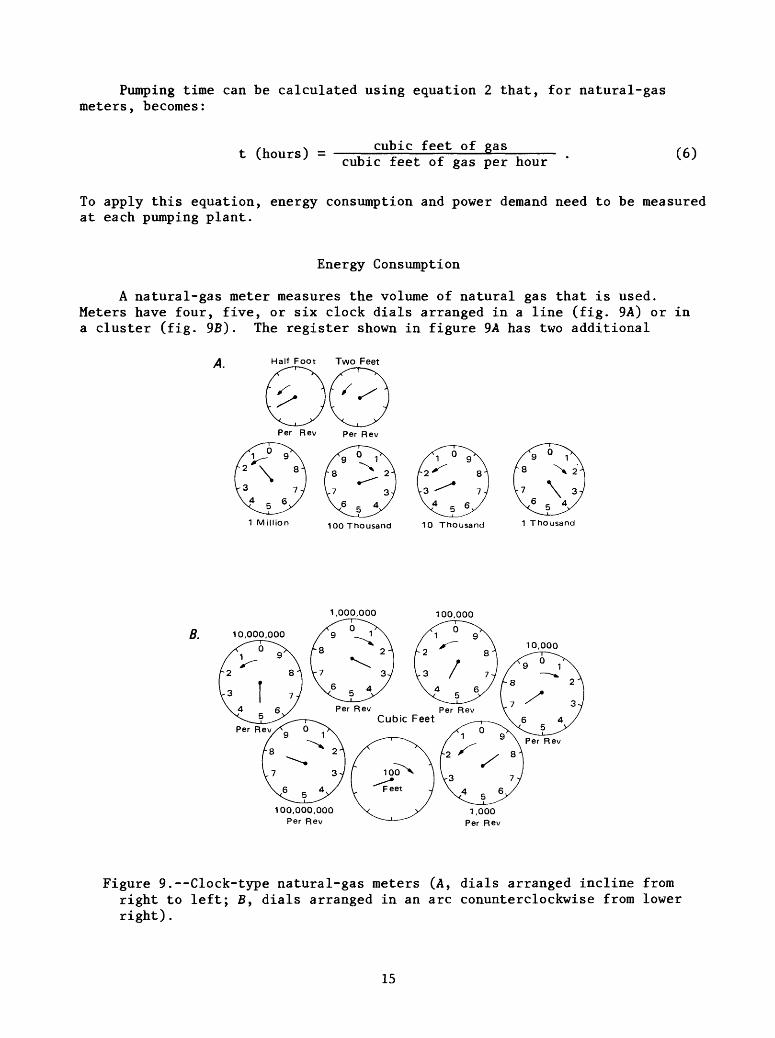
A natural-gas meter measures the volume of natural gas that is used. Meters have four, five, or six clock dials arranged in a line (fig. 9A) or in a cluster (fig. 9B) . The register shown in figure 9A has two additional

A. Half Foot Two Feet

1 Million 100 Thousand 1 Thousand

100,000

B.

100,000,000Per Rev

Figure 9.--Clock-type natural-gas meters (A, dials arranged incline from right to left; B, dials arranged in an arc conunterclockwise from lower right).

15

dials labeled "half foot per rev", and "two feet per rev". The^ measure the gas that passes through the meter at the rate of one half or two cubic feet per revolution. The pointers of the clock dials are driven by a series of interconnecting gears. The pointer that measures the smallest volume of gas metered drives the adjacent pointer that measures "the next larger volume of gas metered, which in turn drives the next adjacent pointer, and so on. Because of the gearing arrangement, each pointer rotates in a direction counter to its neighbors. The two rate-measuring pointers in figure 9A rotate in the same direction, however, due to a connecting gear between them.

Each of the volume-measuring dials is labeled with the volume that represents one complete revolution of the pointer. For instance, for the 1-thousand-ft3 dial, labeled "1000" or "1000 per rev," the pointer makes one complete revolution for every 1,000 ft3 of gas that passes through the meter. Each division on the 1-thousand-ft3 dial represents the passage of 100 ft 3 of gas; each division on the 10-thousand-ft 3 dial represents 1,000 ft3 , and so on.

Careful reading of the pointer of the clock-type meter is needed to ensure that the correct number is recorded. For example, when the pointer for the 10-thousand-ft3 dial is pointing to about 5, representing 5,000 ft 3 , the meter could be indicating a range of about 4,800 and 5,200 ft 3 (fig. 10). Therefore, to correctly determine the reading for the 10-thousand-ft3 dial it is necessary to read the 1-thousand-ft3 dial. If the 1-thousand-ft3 dial reads not yet past 0, for example, 8 or 9, then the 10-thousand-ft3 dial is not yet to 5, so that the reading is 4,800 or 4,900 ft 3 . If the 1-thousand-ft 3

A. Half Foot Two Feet

B.

Cubic Feet

___4__S_JLJL

1 Million

6 c 4 ^ ^

100 Thousand 10 Thousand

Half_Foot TWO Feet

Cubic Feet

1 Thousand

1 Million100 Thousand 10 Thousand 1 Thousand

Figure 10.--Examples of dial readings for clock-type natural gas meters.

16

dial is already past 0, for example, 1 or 2, then the 10-thousand-ft 3 dial is already past 5, so that the reading is 5,100 or 5,200 ft 3 . If the 1-thousand-ft3 dial had read about 0, then the 10-hundred-ft 3 dial, if there is one, would need to be read to determine the position of the 10-thousand-ft 3 dial. An exercise in reading dials used on natural-gas meters is shown in figure 11. The meter readings depicted by the dials in figure 11 are listed in table 3.

Table 3. Values of readings for natural-gas meters shown in figure 11

Figure Cubic feet

11A 423,50011B 775,20011C 490,70011D 708,900

Power Demand

The power demand, or rate of energy consumption, of a pumping point powered by natural gas can be measured by timing the rate at which the pointer smallest-volume dial on the meter rotates while the pump is operating. For the meter arrangement shown in figure 9A, the rate of revolution of the "half foot per rev" dial would be measured; for the meter arrangement shown in figure 9B, the rate of revolution of the "100 feet" dial would be measured. Rate measurements are made by using a stopwatch to time a specified number of revolutions of the pointer. Replicate measurements need to agree within about plus or minus 1 s for a 2 to 3 min test. The power demand is calculated using the following equation:

P = rate x DS x 3,600 , (7)

where P = power demand of pumping-plant installation, in cubic feet ofgas per hour,

rate = average rate of pointer revolution, in revolutions per second, DS = scale of the dial having the pointer that was timed, in cubic

feet of gas per revolution (DS = 0.5 for figure 9A; DS = 100 for figure 9B), and

3,600 = conversion factor (seconds per hour).

Pressure-Correction Factors

Each natural-gas meter operates at a particular pressure controlled by the pressure regulator between the meter and the supply line. For billing purposes, each natural-gas utility company converts the volume of natural gas that passes through a meter into an equivalent volume at the billing pressure.

17

A.Half Foot Two Feet

Cubic Feet

B.

4 c / \ K /!/ \/i e / \6

1 Million 100 Thousand 10 Thousand 1 Thousand

Half Foo\ Two Feet

Cubic Feet

C.

1 Million 100 Thousand

Half Foot Two Feet

10 Thousand 1 Thousand

Cubic Feet

1 Million 100 Thousand 10 Thousand 1 Thousand

Half Foot Two Feet

\Cubic Feet

1 Million 100 Thousand 10 Thousand 1 Thousand

Figure 11.--Meter-reading exercise for clock-type natural-gas meters.

18

The metered volume is converted to the billing volume by multiplying by the pressure-correction factor. Mathematically, the pressure-correction factor (Pc) is

p _ atmospheric pressure + meter pressure ,~>. station pressure + cell constant '

where atmospheric pressure is the average ambient atmospheric pressure at the meter, station pressure is the average ambient atmospheric pressure at the billing office, meter pressure is the operating pressure of the meter as controlled by the regulator, and the cell constant is a pressure drop through the meter. Commonly, atmospheric pressure and station pressure are assumed to be equal. Billing pressure is the sum of the station pressure plus the cell constant. The value of the cell constant is different for different areas. In Colorado, the Public Utilities Commission prescribes the cell constant at 0.25 lb/in2 . When the cell constant is 0, the station pressure is the billing pressure. For example, a gas meter is operated at 20 lb/in2 and has a cell constant of 0.25 lb/in2 . The atmospheric pressure is assumed to be the same as the station pressure, which is 12.99 lb/in2 . The pressure-correction factor then would be:

12 99 + 20 0PC = '^ zu = 2 491712.99 + 0.25 z '^ 1/ '

Pressure-correction factors for various meter pressures, the station pressure, and the cell constant can be obtained from the utility company. The meter pressure used by the utility company for each pumping-plant installation also needs to be obtained from the utility company.

For a service area at about sea level, the station pressure is about 14.70 lb/in2 . For a service area at an altitude of about 4,000 ft, the station pressure is about 12.71 lb/in2 . For a service area at an altitude of about 7,500 ft, the station pressure is about 11.18 lb/in2 . From these dif­ ferences in station pressures, it is obvious that if rates or volumes of natural-gas consumption are to be compared from one service area to another, it first may be necessary to convert all of the values to a common base pressure.

The pressure-correction factor applies to the measured energy consumption and the measured power demand. Therefore, it would appear in both the numer­ ator and the denominator of equation 6 and would not affect the outcome of the pumping-time calculation. However, it is best to adjust for this factor in all reported data so that sites can be compared. Also, in some instances, energy consumption for a site might be obtained from a utility company, whereas power demand might be obtained by onsite measurement; in this instance, the data need to be adjusted to the same pressure before calcu­ lations can be done.

19

Bulk-Supplied Energy

Bulk-supplied energy generally is some form of fuel that is burned in an internal-combustion engine. The common fuels are gasoline and diesel oil, sold by the gallon, and liquid petroleum gas, sold~~by the pound. Calculation of ground-water pumpage from these energy sources requires determination of the total volume of fuel consumed during a given period for an individual pumping plant (energy consumed) and rate of fuel consumption by the pumping plant (power demand).

The volume of fuel consumption can be determined from a log or inventory of the fuel that is used by each individual pumping plant. The rate of fuel consumption is determined by measuring the volume of fuel consumed during a short period of steady, continuous pumping. The volume of gasoline or diesel oil consumed during the test can be determined by measuring the change in depth of the contents of the fuel tank and calculating the volume used from the geometry of the tank or by measuring the volume of fuel required to re-fill the tank to its original level. For fuels sold by weight, the volume measured during the rate test needs to be multiplied by its specific weight to determine the weight per hour of fuel consumption. The specific weight of a fuel can be calculated by multiplying the specific weight of water (62.3 lb/ft3 at ordinary temperatures) by the specific gravity of the fuel.

Pumping time can be calculated from the equation:

, volume (or weight) of fuel consumed /n> hours = T T . &u . ( -3 r . (9) volume (or weight) consumed per hour

ESTIMATING VOLUME OF GROUND-WATER WITHDRAWALS

Once pumping rate has been measured and pumping time has been calcu­ lated, the volume of ground-water withdrawals can be calculated using equation 1. To calculate volume pumped in acre-feet, this equation becomes:

(10)

where V = volume of water pumped, in acre-feet,Q = average pumping rate, in gallons per minute, t = pumping time, in hours, and

5,433 = conversion factor (gallon hours per acre-feet minutes).

Example calculations of ground-water withdrawals for electrically powered and diesel-oil energy are listed in tables 4 and 5.

Often the pumping rate and corresponding power demand at a pumping installation are measured concurrently during a single site visit. If one assumes that the relation between these two quantities is constant, then volume of water pumped at that installation can be calculated for any period in which the total power consumption is known. This process is called

20

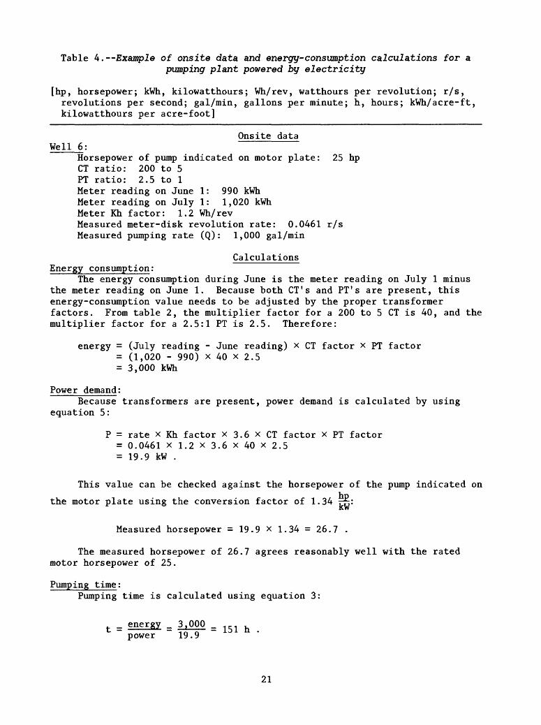
Table 4. Example of onsite data and energy-consumption calculations for apumping plant powered by electricity

[hp, horsepower; kWh, kilowatthours; Wh/rev, watthours per revolution; r/s, revolutions per second; gal/min, gallons per minute; h, hours; kWh/acre-ft, kilowatthours oer acre-footlrevolutions per second; gai/ kilowatthours per acre-foot]

Onsite data Well 6:

Horsepower of pump indicated on motor plate: 25 hpCT ratio: 200 to 5PT ratio: 2.5 to 1Meter reading on June 1: 990 kWhMeter reading on July 1: 1,020 kWhMeter Kh factor: 1.2 Wh/revMeasured meter-disk revolution rate: 0.0461 r/sMeasured pumping rate (Q): 1,000 gal/min

Calculations Energy consumption:

The energy consumption during June is the meter reading on July 1 minus the meter reading on June 1. Because both CT's and PT's are present, this energy-consumption value needs to be adjusted by the proper transformer factors. From table 2, the multiplier factor for a 200 to 5 CT is 40, and the multiplier factor for a 2.5:1 PT is 2.5. Therefore:

energy = (July reading - June reading) x CT factor x PT factor = (1,020 - 990) x 40 x 2.5 = 3,000 kWh

Power demand:Because transformers are present, power demand is calculated by using

equation 5:

P = rate x Kh factor x 3.6 x CT factor x PT factor = 0.0461 x 1.2 x 3.6 x 40 x 2.5 = 19.9 kW .

This value can be checked against the horsepower of the pump indicated on

the motor plate using the conversion factor of 1.34 r~:

Measured horsepower = 19.9 x 1.34 = 26.7 .

The measured horsepower of 26.7 agrees reasonably well with the rated motor horsepower of 25.

Pumping time:Pumping time is calculated using equation 3:

= energy = ^000 = nr»tj*»y 1Q Qpower 19.9

21

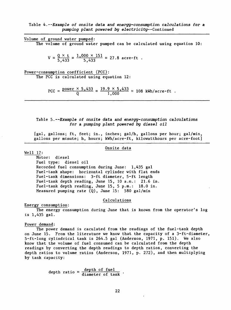
Table 4. Example of onsite data and energy-consumption calculations for a pumping plant powered by electricity Continued

Volume of ground water pumped:The volume of ground water pumped can be calculated using equation 10:

Q x t 1,000 x 151 0 _ 0 r . V = 5^33 = 5,433 = 27 ' 8 acre ' ft '

Power-consumption coefficient (PCC):The PCC is calculated using equation 12:

pcc = power x 5,433 = 19.9^,433 = log kwh/acre. ft .

Table 5. Example of onsite data and energy-consumption calculations for a pumping plant powered by diesel oil

[gal, gallons; ft, feet; in., inches; gal/h, gallons per hour; gal/min, gallons per minute; h, hours; kWh/acre-ft, kilowatthours per acre-foot]

Onsite data Well 17:

Motor: dieselFuel type: diesel oilRecorded fuel consumption during June: 1,435 galFuel-tank shape: horizontal cylinder with flat endsFuel-tank dimensions: 3-ft diameter, 5-ft lengthFuel-tank depth reading, June 15, 10 a.m.: 21.6 in.Fuel-tank depth reading, June 15, 5 p.m.: 18.0 in.Measured pumping rate (Q), June 15: 580 gal/min

Calculations Energy consumption:

The energy consumption during June that is known from the operator's log is 1,435 gal.

Power demand:The power demand is caculated from the readings of the fuel-tank depth

on June 15. From the literature we know that the capacity of a 3-ft-diameter, 5-ft-long cylindrical tank is 264.5 gal (Anderson, 1971, p. 151). We also know that the volume of fuel consumed can be calculated from the depth readings by converting the depth readings to depth ratios, converting the depth ratios to volume ratios (Anderson, 1971, p. 272), and then multiplying by tank capacity:

, ,_, ^. depth of fueldepth ratio = -r-. c- r - .r diameter of tank

22

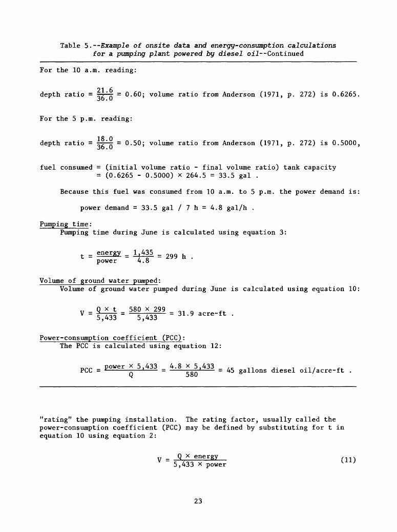
Table 5. Example of onsite data and energy- consumption calculations for a pumping plant powered by diesel oil --Continued

For the 10 a.m. reading:

91 6 depth ratio = |^j = 0.60; volume ratio from Anderson (1971, p. 272) is 0.6265.

For the 5 p.m. reading:

18 0 depth ratio = r^rr = 0.50; volume ratio from Anderson (1971, p. 272) is 0.5000,

fuel consumed = (initial volume ratio - final volume ratio) tank capacity = (0.6265 - 0.5000) x 264.5 = 33.5 gal .

Because this fuel was consumed from 10 a.m. to 5 p.m. the power demand is:

power demand =33.5 gal / 7 h = 4.8 gal/h .

Pumping time:Pumping time during June is calculated using equation 3:

t = = -p- = 299 h . power 4.8

Volume of ground water pumped:Volume of ground water pumped during June is calculated using equation 10

v Q x t 580 x 299 Q1 0 ... v = c /QO = r /oo =31.9 acre-ft . 5,433 5,433

Power-consumption coefficient (PCC) :The PCC is calculated using equation 12:

i>rr power x 5,433 4.8 x 5,433 , c , , , . , . , . ..PCC = * - l = cor. = 45 gallons diesel oil/acre-ft .U joU

"rating" the pumping installation. The rating factor, usually called the power-consumption coefficient (PCC) may be defined by substituting for t in equation 10 using equation 2:

V = Q x energy (n) 5,433 x power ^ }

23

where power is quantified in energy consumption per hour. Re-arranging these terms, and defining the PCC as energy/V, results in the following equation:

PCC = SS^SL = power x 5,433 (12)

where PCC has units of energy consumed per acre-feet of water pumped. Typical values of PCC for pumping plants powered by electricity range from 75 to 150 kWh/acre-ft for open-discharge irrigation wells where ground water is lifted from a depth of less than about 50 ft, to 400 to 500 kWh/acre-ft for pressure systems, such as center-pivot sprinklers, where ground water is lifted from a depth of about 100 ft. Typical values of PCC for pumping plants powered by natural gas range from less than 1,000 ft 3/acre-ft to somewhat more than 10,000 ft 3 /acre-ft. Example calculations of PCC for pumping plants powered by electricity and diesel oil are listed in tables 4 and 5.

As previously stated, the use of a PCC to estimate the volume of water pumped at a site is based on the assumption that the relation is constant between pumping rate and power demand. However, hydrologic and pumping- plant conditions sometimes change, thus altering this relation. For example, pumping head may increase due to drawdown from extensive pumpage, pump effi­ ciency may decrease as the pump ages, and changes in the irrigation-water distribution system may alter the load against which the pump must work. Therefore, pumping rate and power demand need to be verified periodically.

AREA-WIDE ESTIMATION OF GROUND-WATER WITHDRAWALS

There commonly is a need to estimate the volume of ground-water with­ drawals from an area where there are many wells. A variety of methods can be used to make this estimate. Where historical withdrawal estimates are avail­ able for an area, regression can be used to estimate current withdrawals. Luckey (1972) determined that area-wide annual energy consumption is a useful explanatory variable for estimation of area-wide annual ground-water with­ drawals in the Arkansas River valley in Colorado.

Direct measurement of the volume withdrawn from each well in an area will of course produce the best results, but this method becomes impractical where a large number of wells are present. The magnitude of effort can be somewhat decreased by computing the PCC for each well and assuming that it remains constant; records of energy consumption for each well then can be used to calculate total withdrawals. Alternatively, pumping-time measurement devices can be installed at each well, and a representative pumping rate meas­ ured at each well. However, if available personnel and equipment resources are insufficient to measure each well, then a sampling program needs to be undertaken.

In a sampling program, data are collected from a random sample of the total population of wells in the area. Data collected for each well in the sample would include the response variable of interest (either ground-water withdrawal or a surrogate, the PCC), and possible explanatory variables such

24

as source aquifer, irrigation method, energy source, depth to water, pumping rate, and system efficiency. In the simplest instance, a representative value for ground-water withdrawals is calculated from the sample data and multiplied by the number of wells in the area to estimate the area-wide total ground- water withdrawal. Alternatively, a representative value for the PCC is calcu­ lated from the sample data and multiplied by the total power consumption for the area to estimate the area-wide total ground-water withdrawal. The repre­ sentative value used usually is the sample mean; the accuracy to which the sample mean represents the population mean is dependent on the sample size, which can, therefore, be adjusted to obtain the desired estimate accuracy (Luckey, 1972). This calculation also requires that the sample data fit a theoretical population distribution (for example, the normal or log-normal distribution) reasonably well.

In more complex instances, the variability of the ground-water withdrawal data or PCC's will be so large as to limit the usefulness of the sample mean as a representative of the population mean. In these instances, the tech­ niques of analysis of variance (ANOVA) and multiple regression may be used to search for statistically significant explanatory variables.

ANOVA is used where the explanatory variables to be tested are discrete variables, such as source aquifer, irrigation method, and energy source. This method is based on the assumptions that the data for each group are independ­ ent and are normally distributed with equal population variances; it may be necessary to transform the data, or use ranks, in order to meet these assump­ tions. ANOVA will test whether the grouped data have significantly different means. If so, separation of the population into strata will produce improved estimates of total ground-water withdrawal than will use of the ungrouped data.

Multiple regression is used where the explanatory variables to be tested are continuous variables, such as depth to water, pumping rate, and system efficiency. The regression method is based on the assumption that errors (that are approximated by the residuals the differences between the data and the predicted values) are independent and normally distributed with uniform variance. Multiple regression will define the best linear relation between the dependent variable and the explanatory variables. It is helpful to plot the sample data prior to the regression analysis to see whether a linear rela­ tion seems reasonable. After a regression line is developed, it is necessary to check that the errors meet the assumptions (by checking the residuals); transformation of the variables may assist in meeting these assumptions. When a significant regression line is determined, it may be used to predict the ground-water withdrawal (or PCC) for each well in the study area. Unfortu­ nately, the accuracy of these predictions cannot be related to sample size using a single number. The confidence limit for each predicted value depends on sample size, but the relation varies with the magnitude of the explanatory variables.

When explanatory variables are selected, a value for each explanatory variable needs to be assigned for each well in the study area. In practice, explanatory variables should be chosen whose values can be easily determined. It has been documented that pump efficiency is an important factor relating to the PCC and that pump efficiency is highly variable from site to site (Miles

25

and Longenbaugh, 1968). However, the same information that is needed for the standard determination of pump efficiency can be used to determine the PCC directly. It would be advantageous to discover a surrogate variable for pump efficiency that is easier to determine.

SUMMARY AND CONCLUSIONS

Commonly, it is impractical to equip all pumping plants in an area with totalizer flow meters to determine total ground-water withdrawal. A viable alternative is the use of rate-time methods.

Rate-time methods require determination of rate of pumping and time of pumping. Time of pumping can be metered directly or calculated based on energy comsumption and power demand. These calculations use data obtained through reading of energy -meters. Care needs to be taken to read these meters correctly. At pumping plants powered by electricity, the calculations need be modified if transformers are present. At pumping plants powered by natural gas, the effects of the pressure-correction factor need to be included in the calculations. At pumping plants powered by gasoline, diesel oil, or liquid petroleum gas, the geometry of storage tanks needs to be analyzed as part of the calculation.

The relation between power demand and pumping rate at a pumping plant can be described through the use of the power-consumption coefficient. Where equipment and hydrologic conditions are stable, this coefficent can be applied to total energy consumption at a site to estimate total ground-water with­ drawal.

Random sampling of power-consumption coefficients can be used to estimate area-wide ground-water withdrawals. The error of the estimate can be con­ trolled through selection of sample size. In areas where the variability of power-consumption coefficients is large, estimates can be improved by use of analysis of variance or multiple regression. Analysis of variance may reveal significant differences in power-consumption coefficients when data are strat­ ified by source aquifer, energy source, or irrigation method. Multiple regres­ sion may be used to describe linear relations between power-consumption coefficients and continuous explanatory variables, such as pumping rate, depth to water, and pump efficiency.

SELECTED REFERENCES

Addison, Herbert, 1941, Hydraulic measurements: New York, John Wiley, 301 p Allison, S.V., 1967, Cost, precision, and value relationships of data

collection and design activities in water development planning:Berkeley, Calif., University of California Water Resources CenterTechnical Report 6-27, 142 p.

Anderson, K.E., 1971, Water well handbook [1st ed., 9th printing]: Rolla,Mo., Missouri Water Well Drillers Association, 281 p.

26

Baker, C.H., Jr., 1979, Evaluation of methods for estimating ground-waterwithdrawals in western Kansas: U.S. Geological Survey Water-ResourcesInvestigations 79-82, 70 p.

Hayward, A.T.J., 1979, Flowmeters: New York, John Wiley, 197 p. Heimes, F.J., and Luckey, R.R., 1980, Evaluating methods for determining

water use in the High Plains in parts of Colorado, Kansas, Nebraska, NewMexico, Oklahoma, South Dakota, Texas, and Wyoming, 1979: U.S.Geological Survey Water-Resources Investigations 80-111, 118 p.

Johnson Division, 1967, Testing water wells for drawdown and yield: St. Paul,Minn., Bulletin 1243, 8 p.

Kilpatrick, F.A., 1965, Use of flumes in measuring discharge at gagingstations: U.S. Geological Survey Surface Water Techniques, bk. 1,chap. 16, 27 p.

Linford, A., 1961, Flow measurement and meters [2d ed.]: London, E. & F.M.Spon Ltd., 430 p.

Luckey, R.R., 1972, Analyses of selected statistical methods for estimatinggroundwater withdrawal: Water Resources Research, v. 8, no. 1,p. 205-210.

Luckey, R.R., Heimes, F.J., and Gaggiani, N.G., 1980, Calibration and testingof selected portable flowmeters for use on large irrigation systems:U.S. Geological Survey Water-Resources Investigations 80-72, 21 p.

Marella, R.L., and Singleton, V.D., 1988, Metering methods and equipment usedfor monitoring irrigation in the St. Johns River Water ManagementDistrict: Palatka, Fla., St. Johns River Water Management District,17 p.

Miles, D.L., and Longenbaugh, R.L., 1968, Evaluation of irrigation pumpingplant efficiencies and costs in the high plains of eastern Colorado:Fort Collins, Colo., Colorado State University Experiment Station GeneralSeries 876, 19 p.

Ogilbee, William, 1966, Progress report Methods for estimating ground-waterwithdrawals in Madera County, California: U.S. Geological Surveyopen-file report, 42 p.

Ogilbee, William, and Mitten, H.T., 1979, A continuing program for estimatingground-water pumpage in California--Methods: U.S. Geological Surveyopen-file report, 22 p.

Rohwer, Carl, 1942, The use of current meters in measuring pipe discharges:Fort Collins, Colo., Colorado Agricultural Experiment Station TechnicalBulletin 29, 40. p.

Sandberg, G.W., 1966, Two simplified variations of a method for computingground-water pumpage, in Mesnier, G.N., and Chase, E.B., compilers,Selected Techniques in Water Resources Investigations, 1965: U.S.Geological Survey Water-Supply Paper 1822, p. 114-117.

Sudman, Seymour, 1976, Applied sampling: New York, Academic Press, Inc.,249 p.

U.S. Bureau of Reclamation, 1974, Water measurement manual [2d ed., revisedreprint]: Denver, Colo., 326 p. [reprinted 1981 and 1984].

Young, H.W., and Harenberg, W.A., 1971, Ground-water pumpage from the SnakePlain aquifer, southeastern Idaho: Idaho Department of WaterAdministration Water Information Bulletin No. 23, 28 p.

27*U.S. GOVERNMENT PRINTING OFFICE: 1990-0-773-204/20003