Agricultural and Forest Meteorology 209–210 (2015) 36–48

Contents lists available at ScienceDirect

Agricultural and Forest Meteorology

journa l homepage: www.e lsev ier .com/ locate /agr formet

Estimating seasonal variations of leaf area index using litterfallcollection and optical methods in four mixed evergreen–deciduousforests

Zhili Liua, Jing M. Chenb, Guangze Jina,∗, Yujiao Qic

a Center for Ecological Research, Northeast Forestry University, Harbin 150040, Chinab Department of Geography, University of Toronto, Toronto, ON M5S 3G3, Canadac School of Forestry, Northeast Forestry University, Harbin 150040, China

a r t i c l e i n f o

Article history:Received 2 April 2014Received in revised form 20 April 2015Accepted 26 April 2015Available online 16 May 2015

Keywords:Leaf area indexLeaf phenologySeasonal variationLitterfall collectionDigital hemispherical photography (DHP)LAI-2000

a b s t r a c t

Leaf area index (LAI), a critical parameter used in process models for estimating vegetation growth, canbe measured through litterfall collection, which is usually referred to as a direct method. This methodhas been demonstrated to be applicable to deciduous forests, but few studies have used this method forestimating seasonal variations of LAI in mixed evergreen–deciduous forests. In this study, we proposeda practical method to estimate the seasonal variation of LAI directly by combining leaf emergent sea-sonality and litterfall collection (defined as LAIdir) in a mixed broadleaved-Korean pine (Pinus koraiensis)forest (BK), a Korean pine plantation (KP), a spruce–fir valley forest (SV), and a secondary birch (Betulaplatyphylla) forest (SB). In this direct method, the seasonal variation of LAI in a mixed forest can be quan-tified by tracking leaf growth and fall patterns throughout the growing season for each major evergreenand deciduous species. Using the LAIdir as a reference, we validated optical LAI (effective LAI, Le) mea-surements through a digital hemispherical photography (DHP) and the LAI-2000 instrument. We alsoexplored the contribution of major sources of errors to optical LAI, including woody-to-total area ratio(˛), clumping index (˝E), needle-to-shoot area ratio (�E) and automatic exposure (E). We determinedthat DHP Le significantly (P < 0.05) underestimated LAIdir from May to November by 48–64% in BK, KPand SV but overestimated LAIdir by 7% on average in SB. Similarly, LAI-2000 Le also significantly (P < 0.05)underestimated LAIdir by an average of 27–35% in BK, KP and SV but overestimated LAIdir by 22% onaverage in SB. The relative contribution of E to the error in DHP Le is larger than other factors, and the�E was the largest relative contributor to the underestimation of LAI by LAI-2000. The results from ourstudy demonstrate that seasonal variations of LAI in mixed evergreen–deciduous forests can be opticallyestimated with high accuracy (85% for DHP and 91% for LAI-2000), as long as accurate corrections aremade to the various factors mentioned above. These close agreements between direct and optical LAIresults also suggest that the direct method developed in this study is useful for tracking the seasonalvariation of LAI in mixed forests.

© 2015 Elsevier B.V. All rights reserved.

1. Introduction

Leaf area index (LAI), defined as half the total green leaf area perunit ground surface area (Chen and Black, 1992), is one of the mostimportant plant canopy structural parameters that controls fluxesof carbon, energy, and water in terrestrial ecosystems (Weiss et al.,2004; Sonnentag et al., 2007; Behera et al., 2010; Ryu et al., 2012).

∗ Corresponding author. Tel.: +86 451 82191823.E-mail addresses: liuzl2093@126.com (Z. Liu), chenj@geog.utoronto.ca

(J.M. Chen), taxus@126.com (G. Jin), 297148363@qq.com (Y. Qi).

LAI is routinely used to drive process-based canopy photosynthe-sis models (Chen et al., 1999; Silva et al., 2012; Savoy and Mackay,2015). The accuracy of LAI estimation is, therefore, of particularinterest to ecological modelers. Because LAI varies seasonally inboth evergreen and deciduous forests, it is essential to monitor itsseasonal variation to understand the variations that occur in manyforest ecosystem processes (e.g., photosynthesis, respiration, evap-otranspiration, etc.) (Maass et al., 1995; Yan et al., 2012; Hardwicket al., 2015).

Typically, ground-based methods for estimating LAI are segre-gated into direct and indirect methods. LAI derived from directmethods is close to the true LAI and is usually attained through

http://dx.doi.org/10.1016/j.agrformet.2015.04.0250168-1923/© 2015 Elsevier B.V. All rights reserved.

Z. Liu et al. / Agricultural and Forest Meteorology 209–210 (2015) 36–48 37

destructive sampling, allometry, and litterfall collection (Gowerand Norman 1991; Chen et al., 1997; Ryu et al., 2010; Pueschelet al., 2012). However, the destructive method is labor intensive,time-consuming, ruins the samples and is practical only for smallareas. Allometry initially requires destructive sampling to estab-lish allometric relationships, but using relationships established inother regions often leads to inaccuracies. Moreover, the seasonalityof LAI in a forest is almost impossible to monitor using the first twomethods (Bréda, 2003; Macfarlane et al., 2007a). In contrast, thelitterfall collection method is non-destructive. In this case, specificleaf area (SLA), defined as the ratio of area to the mass of an indi-vidual leaf, should be measured accurately. SLA varies with species(particularly between broadleaf and needleleaf species) and alsoexhibits seasonal changes (Grassi et al., 2005; Misson et al., 2006;Poorter et al., 2009; Nouvellon et al., 2010). Therefore, species-specific SLA seasonality should be considered when estimating LAIusing the litterfall collection method. However, most previous stud-ies have excluded the effect of seasonality of SLA on LAI estimation(Neumann et al., 1989; Maass et al., 1995; Kalácska et al., 2005).

The litterfall collection method is more effective when usedin deciduous forests that have a single leaf-fall season than forevergreen or mixed forests, which undergo continuous leaf lossand replacement over longer periods of time (Cutini et al., 1998;Jonckheere et al., 2004; Nasahara et al., 2008). In recent years, tech-niques have been developed to obtain the annual maximum LAI(LAImax) of evergreen coniferous stands by multiplying the fallenLAI during a certain period with needle life span (Sprintsin et al.,2011; Guiterman et al., 2012; Reich et al., 2012). However, the litter-fall collection method only determines the seasonality of LAI duringthe leaf-fall season, as it provides little information about LAI dur-ing the leaf-out season. Recently, Nasahara et al. (2008) addressedthis problem in a deciduous forest by developing a practical methodfor measuring the seasonality of LAI (from May to November) usingboth litterfall collection and periodic in situ observation of sampleshoots. However, few studies have directly measured the sea-sonal dynamics of LAI in evergreen or mixed evergreen–deciduousforests. Liu et al. (2012) monitored the seasonality of LAI in an old-growth, mixed broadleaved-Korean pine (Pinus koraiensis) forestby combining litterfall collection and optical methods with leafseasonality observations in the field. This method assumes thatbroadleaves and needles of each species emerge almost simul-taneously during the leaf-out season. However, Kikuzawa (1983)reported that different species have different leaf emergence char-acteristics, depending on the duration of leaf emergence, whichhas also been observed by several other researchers (e.g., Suzuki,1998; Nasahara et al., 2008; Davi et al., 2011). Therefore, takinginto account interspecific differences in the timing of leaf emer-gence is essential for accurately estimating the seasonal changes ofLAI using the litterfall collection method.

Indirect methods determine LAI from measurements of radia-tion transmission within a canopy using radiative transfer theories(Ross, 1981), and they have been widely adopted because of theirversatility and ease of temporal and spatial replication. The digitalhemispherical photography (DHP) and the LAI-2000 plant canopyanalyzer are two of the most commonly used devices (Chen et al.,2006; Macfarlane et al., 2007b; Chianucci and Cutini, 2013). How-ever, the accuracy of LAI measurements by these indirect methodsusually needs to be checked and calibrated because of their inher-ent limitations; for example, they are often unable to distinguishleaves from woody materials (Chen and Black, 1992) and to quan-tify the clumping effects within canopies (Chen, 1996; Eschenbachand Kappen, 1996; Mason et al., 2012). Therefore, effective LAI (Le),is an alternative term to describe optical LAI estimates (Chen andBlack, 1992). Additionally, a considerable error in DHP LAI measure-ments lies with the automatic exposure setting often used whenphotographing canopies (Chen et al., 1991; Englund et al., 2000;

Pueschel et al., 2012). In general, it has been widely reported thatoptical methods produced lower LAI values than direct methods.For instance, the LAI-2000 Le underestimated destructive LAI by1% (Dufrêne and Bréda, 1995) to 45% (Chason et al., 1991), andVan Gardingen et al. (1999) found the DHP Le underestimated LAIby 50% relative to a harvesting method in a canopy of Gliricidiasepium in Mexico. However, the opposite conclusions have alsobeen reported in previous studies of different forests; Deblondeet al. (1994), for instance, reported that LAI-2000 Le overestimateddirectly harvested LAI by 21–41% in four separate jack pine (P.banksiana) forests, while Whitford et al. (1995) found that hemi-spherical photography overestimated LAI by 73% in dry sclerophylljarrah (Eucalyptus marginata) forests. As those results indicate,there is a large degree of uncertainty when estimating LAI in forestsusing optical methods. Chen (1996) confirmed that optical mea-surements corrected for woody materials and clumping effectscould produce more accurate LAI values in conifer stands than mea-surements obtained from limited destructive sampling. However,the seasonality of LAI derived from indirect methods after con-sidering the effects of woody materials and foliage clumping hasrarely been calibrated against direct measurement of LAI in mixedevergreen–deciduous forests because of the difficulty in obtainingreplicated direct measurements.

The objectives of this study were (1) to develop a directmethod for estimating the seasonal variation in LAI by combin-ing leaf emergent seasonality and the litterfall collection in mixedevergreen–deciduous forests and (2) to evaluate optical methods(DHP and LAI-2000) for estimating the seasonal variation in LAIin mixed evergreen–deciduous forests, as well as to quantify thecontributions of different sources of errors (e.g., woody materials,clumping effects within a canopy, incorrect automatic exposure byDHP) to optical LAI estimation.

2. Materials and methods

2.1. Site description and sample design

The study site was located within the Liangshui National NatureReserve, in Northeastern China (47◦ 10′ 50′′ N, 128◦ 53′ 20′′ E).This site is characterized by a rolling mountainous terrain, rang-ing from 300 m to 707 m above sea level, with a typical slope of10–15◦. The mean annual air temperature is −0.3 ◦C, and the meanair temperature during summer months (from June to August) is17.5 ◦C. The mean annual rainfall is 676 mm, from which 10–20%derives from snowfall, and the area is covered by snowpack fromDecember through April. This area has a long history of commu-nity development with a variety of forest types. It includes not onlythe primary forest at the climax stage but also secondary and artifi-cial forests in different successional stages. These forests are mostlymixed broadleaved-Korean pine forest (BK), Korean pine plantation(KP), spruce–fir valley forest (SV) and secondary birch (Betula platy-phylla) forest (SB), and for our purposes were all classified as mixedevergreen–deciduous forests. Table 1 contains detailed informationabout the forests included in this study.

Permanent dynamic monitoring plots were established in fourforests. Diameter at breast height (DBH), height, and coordinatesof every tree with DBH ≥1 cm in each plot were measured. Theplot area for BK was 160 m × 160 m, and a total of 64 litter trapswere installed on an 8 × 8 grid with 20 m spacing. KP had threesampling plots (each 20 m × 30 m), and each plot was divided into10 m × 10 m subplots. One litter trap was installed at the center ofeach KP subplot, resulting in a total of 18 litter traps for the threeKP plots. Both SV and SB had one sampling plot (60 m × 60 m), with20 litter traps set randomly in each plot. The litter traps were sur-rounded with 8 mm diameter wires and covered with a nylon mesh

38 Z. Liu et al. / Agricultural and Forest Meteorology 209–210 (2015) 36–48

Table 1General status and species composition of four mixed forests under investigation.

Forest types Major species Density Mean DBH BA Relative Land-use Age(trees ha−1) (cm) (m2 ha−1) dominance (%) history (year)

Mixedbroadleaved-Koreanpine forest

Evergreen: Pinus koraiensis 254 30.34 28.22 67 Virgin forest >300Abies nephrolepis, Picea spp.Deciduous: Tilia amurensis 2119 4.65 14.08 33Acer mono, Betula costata

Korean pine plantation Evergreen: Pinus koraiensis 1000 15.24 22.88 69 Afforestation in 1954 60Picea spp.Deciduous: Betula platyphylla 1006 13.30 10.86 31Larix gmelinii

Spruce–fir valley forest Evergreen: Abies nephrolepis 1663 8.98 17.09 67 Virgin forest >300Picea spp.Deciduous:Larix gmelinii

493 10.24 8.34 33

Betula platyphylla

Secondary birch forest Evergreen: Picea spp. 150 11.10 1.86 8 Natural regenerationforest after clearcutting

61Deciduous: Betula platyphylla 2704 7.00 21.14 92Larix gmelinii

(1 mm pore size, 0.5–0.6 m depth). Each litter trap had a 0.5 m2 or1.0 m2 square aperture, and its base was approximately 0.5 m abovethe ground. Leaf litter was collected about every two weeks frommid-August to early November, four times from December to earlyAugust, and once a month from May to August, from early August2011 until early August 2013.

2.2. Direct LAI estimation

Our method for estimating the seasonal trajectory of LAI in amixed evergreen–deciduous forest was to first determine the LAIon 1 May and then track the increasing LAI from the growth ofnew leaves (needles) and the decreasing LAI due to leaf (needle)fall. To calculate the LAI on 1 May we estimated the annual max-imum LAI (LAImax) using the litterfall collection method. To trackthe increased LAI due to new leaf (needle) growth in each period,we estimated the total increased LAI of new leaves (needles) inthe entire growing season (from leaf out to leaf fall) using litterfallcollection and the ratio of the increased LAI for each species to allspecies through periodic leaf emergent seasonality. The decreasedLAI was directly derived from litterfall collection. In this way, theLAI for the entire canopy can then be calculated, from the initialleaf-out to the leaf-fall season.

2.2.1. Seasonality of specific leaf area (SLA)We monitored the seasonal changes of SLA for dominant species

(including 9 deciduous and 3 evergreen species) on 1 August, 1September, 15 September, 1 October, 15 October, and 1 Novemberof 2012. For broadleaf species, 10–70 flat leaves were randomlyselected from the total litter collection in each period. The num-ber varied because fewer leaves were trapped during the early andlate leaf-fall seasons than in the peak growing season. The area ofeach flat leaf was measured with a BenQ-5560 image scanner (BenQCorporation, China, 300 dpi resolution), whereas non-flat leaveswere first flattened by immersing in water. For needleleaf species,we randomly selected 200–400 needles of each species from littertraps, and then measured the total needle area of each species usingthe volume displacement method (Chen, 1996). The areas of sam-ple leaves were recorded, and samples were then dried (for morethan 48 h at 65 ◦C) to a constant weight and weighed to the nearestmilligram. SLA was then calculated using:

SLAj = Aj

Wj(1)

where SLAj is the specific leaf area of species j; Aj is the total leafarea summed for all sampled leaves of species j; and Wj is the totaldry mass summed for all sampled leaves of species j.

2.2.2. Estimation of the annual maximum leaf area index (LAImax)For deciduous species, the LAImax was estimated by measuring

the litter mass of the entire leaf-fall season and converting it to leafarea using the measured SLA for each species. For evergreen species,the LAImax was estimated by first measuring LAI from the litterfallcollection within a certain period (one year) and then multiplyingit by the average needle age (Age) (i.e., needle life span) for eachspecies:

LAImax-2011 =t2∑t1

LAIlitter × Age (2)

where t1 = 1 August 2011 and t2 = 1 August 2012 for BK and KP.Similarly, LAImax-2012 was estimated by the litterfall from 1 August2012 to 1 August 2013. For SV and SB, LAImax occurred in early July,and therefore, one year was defined as 1 July of the previous yearto 1 July of the focal year.

2.2.3. Measurements of needle life spanFor evergreen conifers, the total LAI in the canopy at time t,

LAIcanopy-total (t), regardless of its age, was obtained by:

LAIcanopy-total(t) =n∑

i=1

LAIcanopy,i(t) (3)

where LAIcanopy, i (t) is the LAI of needles of age i in the canopy attime t, and the age of current-year needles is defined as 1. Assum-ing new LAI is the same each year, a measurement of LAIcanopy,

i in any year represents the average condition. Thus, the LAI ofneedles that survived until i − 1 year but died in i year (needlelitter of age i − 1) is LAIcanopy-remain, i-1 − LAIcanopy-remain, i, whereLAIcanopy-remain, i is the remaining LAI in the canopy after i year, andthe ratio of the LAI of needle litter of age i − 1 to the total LAI ofneedles in the canopy equals (LAIcanopy-remain, i-1 − LAIcanopy-remain,

Z. Liu et al. / Agricultural and Forest Meteorology 209–210 (2015) 36–48 39

i)/LAIcanopy-total. The Age is a weighted average of LAI of needle litterof different ages, i.e.:

Age =n∑

i=2

LAIcanopy-remain, i-1 − LAIcanopy-remain,i

LAIcanopy-total× (i − 1)

=n∑

i=2

(LAIcanopy-remain, i-1

LAIcanopy-total− LAIcanopy-remain, i

LAIcanopy-total

)× (i − 1)

=n∑

i=2

(SRi−1 − SRi) × (i − 1)

(4)

where SRi is the survival ratio of needles of age i. The needle SRfor P. koraiensis, Abies nephrolepis, and Picea spp. was measured inthe field from branch samples. For each species, 54 branch sam-ples were taken from three trees: one dominant (D, DBH ≥ 40 cm),one co-dominant (M, 20 ≤ DBH < 40 cm) and one suppressed (S,DBH < 20 cm), at three heights for each tree: top (T), middle (M)and low (L), thus creating nine classes containing six branch sam-ples each: DT, DM, DL, MT, MM, ML, ST, SM, and SL. In the laboratory,all needles were removed from the branches and separated into agegroups (1-year-old, 2-year-old, and so on). We recorded the totalnumber of needles of different ages for each branch sample, fromthe youngest with the largest number of needles to the oldest withjust a few needles. Assuming the number of new needles is the sameeach year, and we then calculated the SR of needles of age i (SRi)using:

SRi = Ni

N1(5)

where Ni is the number of needles of i-year-old and N1 is the num-ber of needles of age 1. Substitutions for SR in Eq. (4) then yield toAge of each needleleaf species. The Age of each species in the standwas derived by weighting the mean age in each of the three DBHclasses against the total basal area of the species in each class.

2.2.4. Leaf (needle) emergent seasonality during the leaf-outseason

We determined leaf (needle) emergent seasonality throughperiodic in situ observation of sample shoots. The observationswere conducted for 14 species (10 deciduous broadleaf, 3 ever-green needleleaf and 1 deciduous needleleaf species) on 1 May,15 May, 1 June, 15 June, 1 July, 15 July, and 1 August of 2012. Forbroadleaf species, we sampled 30 shoots from 30 trees of 10 species(three trees per species). During each period, we obtained the fol-lowing observations for each sample shoot: (1) the number of newleaves (i.e., those that emerged since the prior measurement dateand were longer than 0.5 cm) and (2) the size (length and width) ofall leaves. We calculated the total leaf area of a shoot at time t foreach species (i.e., LAtotal (t)) as

LAtotal(t) =n∑

k=1

Lk(t) × Dk(t) × m (6)

where Lk (t) is the leaf length of leaf k at time t; Dk (t) is the leafwidth of leaf k at time t; and m is the adjustment coefficient toaccount for the irregular shape of leaves that referred to Liu et al.(2012).

The increased ratio for the total leaf area per shoot at time t (i.e.,R(t)) was obtained from:

R(t) = LAtotal(t)LAtotal−max

(7)

where LAtotal (t) is defined in Eq. (6), and LAtotal-max is the annualmaximum total leaf area per shoot. The R (t) data were used torepresent the ratio of LAI at time t to LAImax. Thus, the seasonal

changes of LAI for each broadleaf species during the leaf-out seasonwere obtained by multiplying the LAImax by the ratio.

For needleleaf species, we selected 240 shoots from 12 trees of4 species (20 shoots were randomly selected per tree). During thesame observation period as broadleaf species, each sample shootwas observed for (1) needle length (5–10 needles per shoot wererandomly selected for determining the mean needle length); (2)shoot length; and (3) the number of needles per unit length ofthe shoot. The tips of needles were acuminate, and therefore, theirareas were negligible. Thus, the needles of P. koraiensis approxi-mate triangular prisms, whereas those of Picea spp., A. nephrolepisand Larix gmelinii are cuboid. The cross-sections are equilateral tri-angles for P. koraiensis, squares for Picea spp., and rectangles forboth A. nephrolepis and L. gmelinii. The total needle area per shootat time t (i.e., NAtotal (t)) of each species was calculated using:

NAtotal(t) = 3a × Ln(t) × Nu(t) × Ls(t) for Pinus koraiensis (8)

NAtotal(t) = 4a × Ln(t) × Nu(t) × Ls(t) for Picea spp. (9)

NAtotal(t) = 2(b + c) × Ln(t) × Nu(t) × Ls(t) for Abies nephrolepis (10)

NAtotal(t) = 2(b + c) × Ln(t) × Nu(t) × Ls(t) for Larix gmelinii (11)

where a is the side of the cross section, averaging 1.00 mm for P.koraiensis and 0.98 mm for Picea spp.; b is the width of the needle,averaging 1.33 mm for A. nephrolepis and 0.60 mm for L. gmelinii,respectively; c is the thickness of the needle, averaging 0.44 mmfor A. nephrolepis and 0.32 mm for L. gmelinii, respectively; Ln(t) isthe mean length of the needle at time t; Nu(t) is the number ofneedles per unit length of shoot at time t; and Ls(t) is the length ofthe shoot at time t.

We determined the increased ratio for the needle area duringeach leaf-out season similar to that for the broadleaf species byusing Eq. (7). However, the ratio data could only be used to rep-resent the temporal variation pattern of the increased LAI of newneedles during the leaf-out season (�LAI) and does not representthe total LAI as with broadleaf species because evergreen needlesalso fall when the new needles are produced during the leaf-outseason. To obtain the total �LAI of new needles in 2012 (�LAItotal),we first calculated the LAI for each evergreen needleleaf species on1 May 2012 (LAIMay-2012) using:

LAIMay−2012 = LAImax−2011 −t2∑t1

LAIlitter(t) (12)

wheret2∑t1

LAIlitter(t) is the summation of LAI of needle litter from

time t1 to t2, where t1 = Aug-2011 and t2 = May-2012. We assumedthat no new needles were produced from August to May.

The LAI for each evergreen needleleaf species on 1 November2012 (LAINov-2012) was subsequently calculated by the equation:

LAINov−2012 = LAImax-2012 −t2∑t1

LAIlitter(t) (13)

wheret2∑t1

LAIlitter(t) is the summation of LAI of the needle litter

from time t1 to t2, where t1 = Aug-2012 and t2 = Nov-2012.The four forests were considered to be evergreen needleleaf

forests before 1 May and after 1 November because almost no broadleaves were in the canopies outside of the growing season. Thus, the

40 Z. Liu et al. / Agricultural and Forest Meteorology 209–210 (2015) 36–48

�LAItotal for each evergreen needleleaf species during the leaf-outseason was calculated as:

�LAItotal = LAINov−2012 +t2∑t1

LAIlitter(t) − LAIMay−2012 (14)

where LAINov-2012 and LAIMay-2012 are defined in Eqs. (12) and (13),

andt2∑t1

LAIlitter(t) is the summation of LAI of the needle litter from

time t1 to t2, where t1 = May-2012 and t2 = Nov-2012.We could then obtain the LAI for each evergreen needleleaf

species at time t (i.e., LAI (t)) during the leaf-out season by using:

LAI(t) = LAIMay−2012 + �LAItotal × R(t) −t∑

t1

LAIlitter(t) (15)

where R(t) is the increased ratio for the needle area at time t, and∑tt1LAIlitter(t) is the summation of LAI of the needle litter from

time t1 to t, where t1 = May-2012. By adding the component LAIof all deciduous and evergreen species, we determined the overallseasonality of LAI for each forest during the leaf-out season.

2.2.5. Leaf (needle) fall seasonality during the leaf-fall seasonFor all forests, based on the LAImax, we determined the season-

ality of LAI during the leaf-fall season by deducting the decreasedLAI from the total litter of all species during each leaf-fall season.The decreased LAI was calculated by multiplying the litter mass ofeach species by their SLA for that period and dividing that valueby the area of the litter trap. Finally, the seasonal variation of LAIduring the entire study periods in each forest was calculated. Inthe present study, the LAI derived from the proposed method wasdefined as direct LAI (LAIdir).

2.3. Indirect LAI estimation (optical methods)

2.3.1. DHP and LAI-2000A digital hemispherical photography (DHP, Nikon Coolpix 4500

digital camera with a 180◦ fish-eye lens) and a LAI-2000 PlantCanopy Analyzer (LI-COR Inc., Lincoln, NE, USA) were used to esti-mate the seasonality of LAI in the four forests at two-week intervalsfrom 1 May to 1 November of 2012. The hemispherical photographsof sample points were taken 1.3 m above the ground. We avoidedtaking photographs under direct solar beam conditions wheneverpossible, with automatic exposure. A total of 832 hemispheric pho-tographs were obtained in BK, 234 in KP, and 260 in each of SVand SB. A LAI-2000 unit was operated subsequently at the samephotographic spot for comparison with DHP. The second LAI-2000unit, cross-calibrated with the former, was used to automaticallyrecord “above-canopy” readings from a nearby clearing. A 45◦ field-of-view cap was used on both units to avoid the influence of theoperator on the sensor. The same number of photographs as inthe DHP method were collected by LAI-2000 in the four forests.The hemispherical photographs were processed with DHP softwareto derive the Le (Leblanc et al., 2005; Chianucci et al., 2014), withzenith angle ranging from 45◦ to 60◦. The LAI-2000 data were alsoprocessed using the C2000 software with zenith angle ranges of45–60◦.

2.3.2. Correction of optical LAI estimatesBased on previous theoretical development and validation

(Chen, 1996; Chen et al., 1997), the following equation was usedfor obtaining LAI based on Le:

LAI = (1 − ˛)Le�E

˝E(16)

where ˛ is the woody-to-total area ratio representing the contribu-tion of woody materials to Le; ˝E is the clumping index quantifyingthe effect of foliage clumping at scales larger than shoots; and �Eis the needle-to-shoot area ratio quantifying the effect of foliageclumping within shoots. For broadleaf species, individual leaves areconsidered as foliage elements and thus �E = 1.0, but for needleleafspecies, �E is usually larger than 1.0.

The remaining major challenge in optical LAI measurementslies with determining parameters other than Le in Eq. (16). Inthe present study, Photoshop software (PS) was used to calcu-late ˛ (woody-to-total area ratio) for each study period in themixed evergreen–deciduous forests. First, we obtained Le of thephotograph in a study period using the DHP software. Second,the Clone Stamp Tool in PS was used to replace green materials(mainly leaves and needles) with sky, leaving just tree trunks andlarge branches on the images, following which the woody areaindex (WAI) of the photograph could be obtained by once againusing the DHP software. The ˛ value was then derived accordingly(˛ = WAI/Le), and finally, the seasonality of ˛ was obtained for allmixed evergreen–deciduous forests.

The seasonality of ˝E for each forest was calculated via the DHP-TRAC software (Chen et al., 2006) with zenith angle ranging from40◦ to 45◦. The seasonality of �E for the four forests was measuredin the field. First, the �E for four conifer species (P. koraiensis, A.nephrolepis, Picea spp. and L. gmelinii) was quantified once a monthfrom May to November in 2012. The sample scheme was the sameas that for measuring the Age values. For each needleleaf species,27 shoot samples were taken from three trees. These sample shootswere analyzed according to the volume replacement method pro-posed by Chen (1996). The �E for each forest stand was derived byweighting the �E of the trees of different species by their relativecontribution to total basal area in the stand:

�E(t) =∑

[�j(t) × BAj(t)]∑BAj(t)

(17)

where �E(t) is the �E for the forest at time t; �j(t) is the �E for jspecies at time t; and BAj(t) is the basal area for j species at time t.To obtain the basal area for all species (both evergreen and decidu-ous species) in each study period, we first measured the maximumbasal area for each species based on a subplot survey. Second, theratio of LAI for each species during each observation period (fromMay to November) to LAImax was obtained, so that it was 1.0 atthe seasonal peak LAI, and these ratios were used to represent theseasonal dynamics of basal area. The basal area in each period wasthen calculated by multiplying the maximum basal area with thecorresponding ratio.

In comparison to the LAI-2000 instrument, the accuracy of LAIestimated using the DHP method is affected by the additional issueof photograph exposure setting because it influences the differen-tiation between green leaves and the background (sky). Therefore,for each photograph, we corrected a systematic error due to incor-rect automatic photographic exposure (corrected by E) based onthe relationship between DHP Le obtained with automatic exposureand LAI-2000 Le reported by Zhang et al. (2005).

2.3.3. Bias analysisFor the DHP method, the biases of LAI measurement were caused

by ˛, ˝E, �E, and E, thus LAI = fDHP (˛, ˝E, �E, E). We then calculatedthe total bias (ıLAI) (Topping, 1972):

ıLAI = ∂LAI∂˛

× ı˛ + ∂LAI∂˝E

× ı˝E + ∂LAI∂�E

× ı�E + ∂LAI∂E

× ıE (18)

where ı� = 0 − �; ı˝E = 1 − ˝E; ı�E = 1 − �E; and ıE = 1 − E. The

�, ˝E, �E and E was the mean of each parameter during all studyperiods (from May to November).

Z. Liu et al. / Agricultural and Forest Meteorology 209–210 (2015) 36–48 41

For the LAI-2000 method, the biases of LAI measurement werecaused by ˛, ˝E, and �E, thus LAI = fLAI-2000 (˛, ˝E, �E). We thencalculated the total bias:

ıLAI = ∂LAI∂�

× ı� + ∂LAI∂˝E

× ı˝E + ∂LAI∂�E

× ı�E (19)

The calculation of ı�, ı˝E and ı�E were the same as Eq. (18).

3. Results

3.1. Seasonal changes of SLA

The mean SLA values for major species ranged from 59.41 ± 9.70(mean ± SD) cm2 g−1 to 350.67 ± 8.56 cm2 g−1 in the four forests(Table 2). The SLA values of the broadleaf species were all largerthan those of the needleleaf species. L. gmelinii had a larger SLAvalue than any of the three evergreen needleleaf species. The SLAof most species exhibited significant seasonal trends (P < 0.05), butthe coefficients of variation (CV) were all lower than 19%.

3.2. Measurements of Age

For P. koraiensis, 36.0% of the total needles lived for more thanthree years, but only 4.0% lived for more than four years, and its Agewas 3.07 (Fig. 1). For Picea spp., 40.7% of the total needles lived formore than four years, and only 0.3% of those needles lived for morethan eight years, and its Age was 3.91 (Fig. 1). For A. nephrolepis,52.0% of the total needles lived for more than three years, but only0.9% of the needles lived for seven years, and its Age was 3.70(Fig. 1).

3.3. Leaf (needle) emergent seasonality

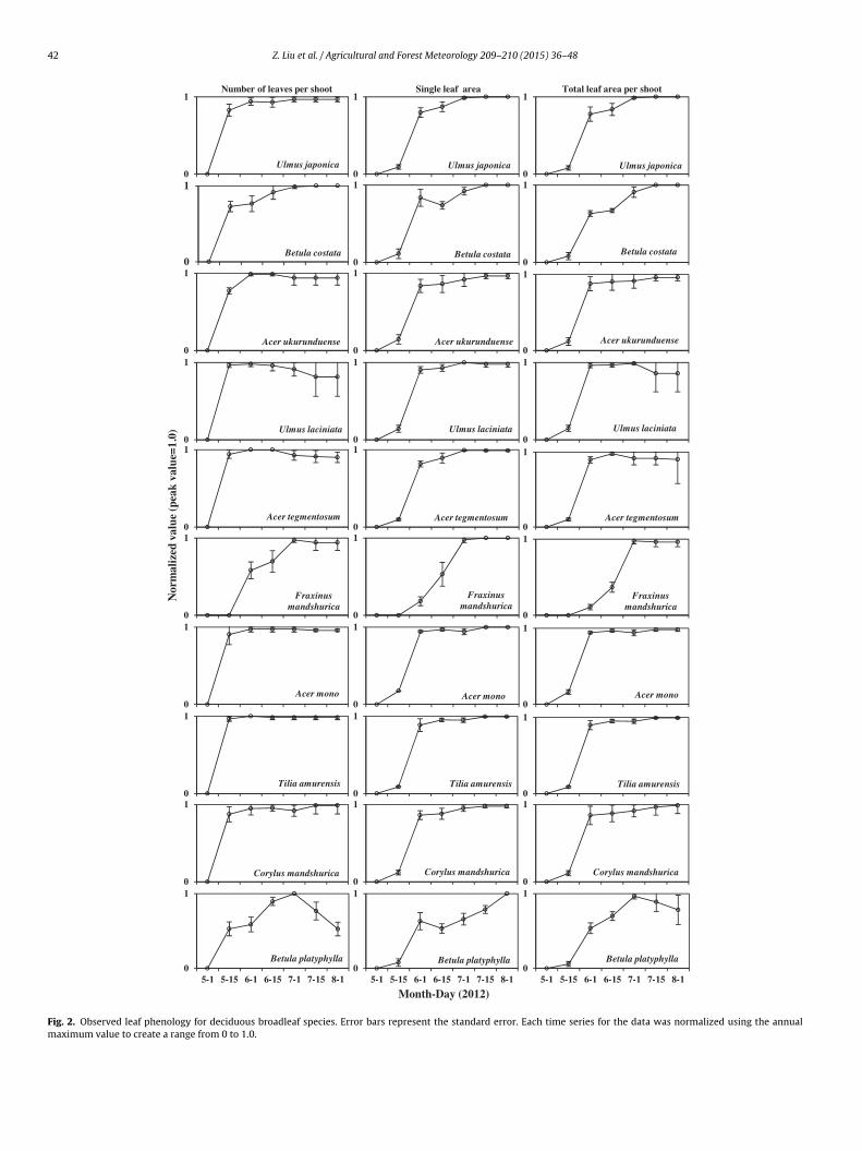
Each species showed a clear seasonality in the leaf (needle) num-ber, single leaf (needle) area, and total leaf (needle) area per shoot(Figs. 2 and 3). Leaves of most broadleaf species emerged in earlyMay except for those of Fraxinus mandshurica, which emerged aftermid-May. Most broadleaf species (except B. platyphylla and F. mand-shurica) showed a flush of leaf emergence (i.e., a rapid emergence ofleaves) in early May and more than 95% (except 76% for B. costata)of total leaves emerged before early June (left column of Fig. 2).B. platyphylla showed two leaf flushes, the first one in early Mayand the second in early June. Because of the small amount of newleaves that emerged during the second flush, the mean single-leafarea of B. platyphylla decreased in mid-June, but recovered with thegrowth of small leaves in the second flush. For B. platyphylla, leavesbegan to fall in early July, and these accounted for 47% of the totalleaves before early August. Most species except U. laciniata and B.platyphylla had a maximum total leaf area per shoot in mid-July(right column of Fig. 2).

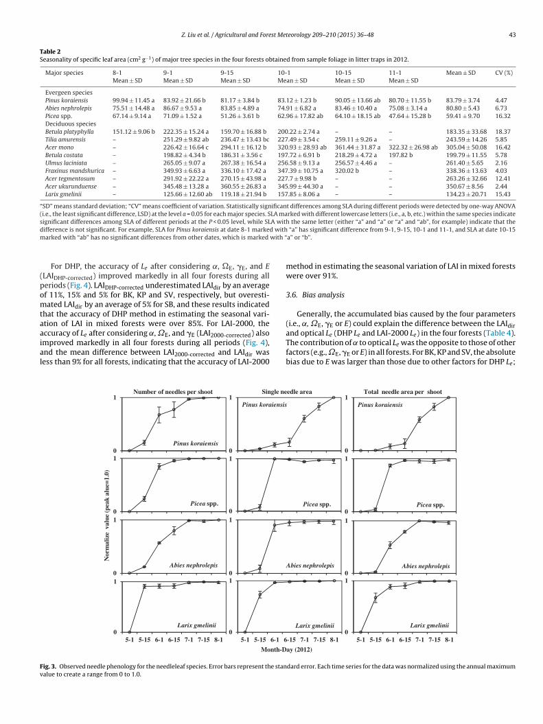
Needleleaf species had a single flush of needle emergence, whichwas about two weeks later than that of the deciduous species (L.gmelinii) (left column of Fig. 3). Most needleleaf species attainedmore than 90% of their largest single needle areas in early June,with the exception of P. koraiensis, for which this occurred in earlyAugust. The single needle area of Picea spp. decreased slightly aftermid-June, probably due to insect herbivory. Total needle area pershoot was highest for all needleleaf species in early August.

3.4. Woody materials and clumping effects on optical LAIestimation

In all forests, the ˛ value showed obvious seasonal variations,and the smallest CV was 24% for SV (Table 3). Generally, the largestmean ˛ was found in SB, with a value of 23 ± 22% (mean ± SD).There was no marked difference in ˛ among BK, KP and SV, with

Fig. 1. The needle survival ratio of different evergreen needleleaf species.

mean values of 6–10%. The seasonal variation of ˝E was small inthese forests, as indicated by the CV values (Table 3). The averageclumping effects on the canopy level for SV (mean value 0.87) wasmuch larger than for other forests. There was no obvious seasonal-ity in �E for all forests, with CV values of 3.50–6.52% (Table 3). Thelargest mean �E (1.49 ± 0.08) was in KP, followed by 1.43 ± 0.09,1.23 ± 0.04 and 1.14 ± 0.07 in BK, SV, and SB, respectively.

3.5. LAI estimation using direct and indirect methods

DHP Le significantly (P < 0.05) underestimated LAIdir during allperiods, by an average of 61% (with the range being 56–65%),64% (55–68%), and 48% (41–53%) for BK, KP and SV, respec-tively (Fig. 4 and Appendix A). Similarly, LAI-2000 Le significantly(P < 0.05) underestimated LAIdir by an average of 35% (22–40%), 27%(19–38%), and 28% (19–33%) for BK, KP and SV, respectively. ForSB, Le from both DHP and LAI-2000 significantly (P < 0.05) overes-timated LAIdir in the early leaf-out and late leaf-fall season (e.g., 1May 15 May 15 October or 1 November). This is due to the contri-bution of woody materials to the radiation interception measuredby optical instruments during these periods. During all periods inSB, DHP Le overestimated LAIdir by an average of 7%, and LAI-2000Le overestimated LAIdir by 22% on average.

42 Z. Liu et al. / Agricultural and Forest Meteorology 209–210 (2015) 36–48

0

1

Ulmus japonica

0

1

Betula costata

0

1

Acer ukurunduense

0

1

Ulmus laciniata

0

1

Acer tegmentosum

0

1

Fraxinus mandshurica

0

1

Acer mono

0

1

Tilia amurensis

0

1

Corylus mandshurica

0

1

5-1 5-15 6-1 6-15 7-1 7-15 8-1

Betula platyphylla0

1

5-1 5-15 6-1 6-15 7-1 7-15 8-1

Betula platyphylla0

1

5-1 5-15 6-1 6-15 7-1 7-15 8-1

Betula platyphylla

0

1

Corylus mandshurica0

1

Corylus mandshurica

0

1

Tilia amurensis0

1

Tilia amurensis

0

1

Acer mono0

1

Acer mono

0

1

Fraxinus mandshurica

0

1

Fraxinus mandshurica

0

1

Acer tegmentosum0

1

Acer tegmentosum

0

1

Ulmus laciniata0

1

Ulmus laciniata

0

1

Acer ukurunduense0

1

Acer ukurunduense

0

1

Betula costata0

1

Betula costata

0

1

Ulmus japonica0

1

Ulmus japonica

Number of leaves per shoot Single leaf area Total leaf area per shoot

Nor

mal

ized

val

ue (p

eak

valu

e=1.

0)

Month-Day (2012)

Fig. 2. Observed leaf phenology for deciduous broadleaf species. Error bars represent the standard error. Each time series for the data was normalized using the annualmaximum value to create a range from 0 to 1.0.

Z. Liu et al. / Agricultural and Forest Meteorology 209–210 (2015) 36–48 43

Table 2Seasonality of specific leaf area (cm2 g−1) of major tree species in the four forests obtained from sample foliage in litter traps in 2012.

Major species 8-1 9-1 9-15 10-1 10-15 11-1 Mean ± SD CV (%)Mean ± SD Mean ± SD Mean ± SD Mean ± SD Mean ± SD Mean ± SD

Evergeen speciesPinus koraiensis 99.94 ± 11.45 a 83.92 ± 21.66 b 81.17 ± 3.84 b 83.12 ± 1.23 b 90.05 ± 13.66 ab 80.70 ± 11.55 b 83.79 ± 3.74 4.47Abies nephrolepis 75.51 ± 14.48 a 86.67 ± 9.53 a 83.85 ± 4.89 a 74.91 ± 6.82 a 83.46 ± 10.40 a 75.08 ± 3.14 a 80.80 ± 5.43 6.73Picea spp. 67.14 ± 9.14 a 71.09 ± 1.52 a 51.26 ± 3.61 b 62.96 ± 17.82 ab 64.10 ± 18.15 ab 47.64 ± 15.28 b 59.41 ± 9.70 16.32Deciduous speciesBetula platyphylla 151.12 ± 9.06 b 222.35 ± 15.24 a 159.70 ± 16.88 b 200.22 ± 2.74 a – – 183.35 ± 33.68 18.37Tilia amurensis – 251.29 ± 9.82 ab 236.47 ± 13.43 bc 227.49 ± 3.54 c 259.11 ± 9.26 a – 243.59 ± 14.26 5.85Acer mono – 226.42 ± 16.64 c 294.11 ± 16.12 b 320.93 ± 28.93 ab 361.44 ± 31.87 a 322.32 ± 26.98 ab 305.04 ± 50.08 16.42Betula costata – 198.82 ± 4.34 b 186.31 ± 3.56 c 197.72 ± 6.91 b 218.29 ± 4.72 a 197.82 b 199.79 ± 11.55 5.78Ulmus laciniata – 265.05 ± 9.07 a 267.38 ± 16.54 a 256.58 ± 9.13 a 256.57 ± 4.46 a – 261.40 ± 5.65 2.16Fraxinus mandshurica – 349.93 ± 6.63 a 336.10 ± 17.42 a 347.39 ± 10.75 a 320.02 b – 338.36 ± 13.63 4.03Acer tegmentosum – 291.92 ± 22.22 a 270.15 ± 43.98 a 227.7 ± 9.98 b – – 263.26 ± 32.66 12.41Acer ukurunduense – 345.48 ± 13.28 a 360.55 ± 26.83 a 345.99 ± 44.30 a – – 350.67 ± 8.56 2.44Larix gmelinii – 125.66 ± 12.60 ab 119.18 ± 21.94 b 157.85 ± 8.06 a – – 134.23 ± 20.71 15.43

“SD” means standard deviation; “CV” means coefficient of variation. Statistically significant differences among SLA during different periods were detected by one-way ANOVA(i.e., the least significant difference, LSD) at the level a = 0.05 for each major species. SLA marked with different lowercase letters (i.e., a, b, etc.) within the same species indicatesignificant differences among SLA of different periods at the P < 0.05 level, while SLA with the same letter (either “a” and “a” or “a” and “ab”, for example) indicate that thedifference is not significant. For example, SLA for Pinus koraiensis at date 8-1 marked with “a” has significant difference from 9-1, 9-15, 10-1 and 11-1, and SLA at date 10-15marked with “ab” has no significant differences from other dates, which is marked with “a” or “b”.

For DHP, the accuracy of Le after considering ˛, �E, �E, and E(LAIDHP-corrected) improved markedly in all four forests during allperiods (Fig. 4). LAIDHP-corrected underestimated LAIdir by an averageof 11%, 15% and 5% for BK, KP and SV, respectively, but overesti-mated LAIdir by an average of 5% for SB, and these results indicatedthat the accuracy of DHP method in estimating the seasonal vari-ation of LAI in mixed forests were over 85%. For LAI-2000, theaccuracy of Le after considering ˛, ˝E, and �E (LAI2000-corrected) alsoimproved markedly in all four forests during all periods (Fig. 4),and the mean difference between LAI2000-corrected and LAIdir wasless than 9% for all forests, indicating that the accuracy of LAI-2000

method in estimating the seasonal variation of LAI in mixed forestswere over 91%.

3.6. Bias analysis

Generally, the accumulated bias caused by the four parameters(i.e., ˛, ˝E, �E or E) could explain the difference between the LAIdirand optical Le (DHP Le and LAI-2000 Le) in the four forests (Table 4).The contribution of ˛ to optical Le was the opposite to those of otherfactors (e.g., ˝E, �E or E) in all forests. For BK, KP and SV, the absolutebias due to E was larger than those due to other factors for DHP Le;

0

1

5-1 5-15 6-1 6-15 7-1 7-15 8-1

Larix gmelinii0

1

5-1 5-15 6-1 6-15 7-1 7-15 8-1

Larix gmelinii0

1

5-1 5-15 6-1 6-15 7-1 7-15 8-1

Larix gmelinii

0

1

Pinus koraiensis0

1Pinus koraiensis

0

1

Picea spp.0

1

Picea spp.

0

1

Abies nephrolepis0

1

Abies nephrolepis0

1

Abies nephrolepis

0

1

Picea spp.

0

1Pinus koraiensis

Number of needles per shoot Single needle area Total needle area per shoot

Nor

mal

ize

val

ue (p

eak

alue

=1.0

)

Month-Day (2012)

Fig. 3. Observed needle phenology for the needleleaf species. Error bars represent the standard error. Each time series for the data was normalized using the annual maximumvalue to create a range from 0 to 1.0.

44 Z. Liu et al. / Agricultural and Forest Meteorology 209–210 (2015) 36–48

0

2

4

6

8

10

12LAI from direct method Effective LAI from DHP Effective LAI from LAI-2000Corrected LAI from DHP Corrected LAI from LAI-2000

0

2

4

6

8

10

0

1

2

3

4

5

0

1

2

3

4

5-1 5-15 6-1 6-15 7-1 7-15 8-1 8-15 9-1 9-15 10-1 10-15 11-1

BK

KP

SV

SB

LA

IL

AI

LA

IL

AI

Month-day (2012)

Fig. 4. Seasonal variations of leaf area index (LAI) derived from different methods in the mixed broadleaved-Korean pine forests (BK), Korean pine plantation forest (KP),spruce–fir valley forest (SV), and secondary birch forest (SB). Corrected LAI from DHP is the effective LAI from DHP after correcting for the woody-to-total area ratio (˛),clumping index (˝E), needle-to-shoot area ratio (�E) and automatic exposure (E); and corrected LAI from LAI-2000 is the effective LAI from LAI-2000 after correcting for ˛,˝E and �E. Error bars represent the standard deviations.

Z. Liu et al. / Agricultural and Forest Meteorology 209–210 (2015) 36–48 45

Table 3The observed seasonality of the woody-to -total area ratio (˛), clumping index (˝E) and needle-to-shoot area ratio (�E) in the four forests.

Month-day BK KP SV SB

˛ (%) ˝E �E ˛ (%) ˝E �E ˛ (%) ˝E �E ˛ (%) ˝E �E

5-1 11 0.92 1.41 14 0.96 1.44 13 0.86 1.21 58 0.91 1.275-15 9 0.93 1.38 13 0.93 1.40 11 0.92 1.21 41 0.93 1.186-1 4 0.94 1.28 6 0.97 1.38 8 0.88 1.28 6 0.95 1.116-15 5 0.93 1.28 7 0.97 1.36 11 0.87 1.28 5 0.94 1.097-1 3 0.92 1.39 4 0.95 1.45 10 0.85 1.21 4 0.94 1.077-15 4 0.94 1.40 5 0.93 1.46 9 0.86 1.21 5 0.93 1.088-1 3 0.94 1.47 3 0.95 1.53 7 0.85 1.27 4 0.94 1.118-15 4 0.93 1.48 8 0.96 1.56 6 0.88 1.27 8 0.93 1.139-1 3 0.92 1.45 7 0.95 1.55 9 0.87 1.26 9 0.95 1.209-15 6 0.92 1.48 10 0.96 1.56 8 0.88 1.19 12 0.91 1.1010-1 9 0.92 1.50 8 0.94 1.53 10 0.87 1.15 29 0.93 1.0810-15 10 0.91 1.57 10 0.94 1.57 12 0.87 1.17 54 0.91 1.1611-1 10 0.90 1.57 12 0.92 1.61 14 0.86 1.21 59 0.86 1.30Mean 6 0.92 1.43 8 0.95 1.49 10 0.87 1.23 23 0.93 1.14SD 3 0.01 0.09 3 0.02 0.08 2 0.02 0.04 22 0.02 0.07CV (%) 50 1.28 6.38 42 1.63 5.51 24 2.06 3.50 99 2.43 6.52

“SD” means standard deviation; “CV” means coefficient of variation. BK: mixed broadleaved-Korean pine forest (BK).KP: Korean pine plantation forest, SV: spruce–fir valley forest, and SB: secondary birch forest, the same below.

Table 4The mean difference between the LAI from the direct method (LAIdir) and effective LAI from DHP (DHP Le) or LAI-2000 (LAI-2000 Le), and the biases caused by woody-to-totalarea ratio (˛), clumping index (˝E), needle-to-shoot area ratio (�E) or automatic exposure (E) for optical methods during all study periods in the four forests.

Forests Difference Bias due to ˛ Bias due to ˝E Bias due to �E Bias due to E Total bias

BK −4.27a 0.40 −0.50 −1.83 −2.21 −4.14−2.54b 0.42 −0.52 −1.93 – −2.03

KP −3.94a 0.43 −0.26 −1.58 −1.62 −3.03−1.74b 0.57 −0.35 −2.11 – −1.88

SV −1.92a 0.41 −0.52 −0.68 −1.17 −1.97−1.10b 0.39 −0.51 −0.66 – −0.77

SB −0.36a 0.49 −0.14 −0.22 −0.30 −0.160.07b 0.53 −0.15 −0.23 – 0.15

Difference = DHP Le or LAI-2000 Le − LAIdir.Total bias is the summary of the bias due to each parameter (i.e., ˛, ˝E, �E, or E), and the bias due to each parameter was calculated through Eqs. (18) and (19).

a Meant the mean difference between DHP Le or LAI-2000 Le and LAIdir during all study periods in each forest.b Meant the mean difference between DHP Le or LAI-2000 Le and LAIdir during all study periods in each forest.

and the absolute bias due to �E was larger than those of ˛ and ˝Efor LAI-2000 Le. For SB, the ˛ value was the largest contributor ofuncertainty for both DHP Le and LAI-2000 Le, probably because ofthe variable contribution of woody materials.

4. Discussion

4.1. Reliability of the proposed direct method

Our proposed method directly determined the seasonality of LAIin four mixed evergreen–deciduous forests. Leaf emergent season-ality from sample trees is one of the three most important factorsfor improving the accuracy of the proposed method, and the moretrees that are sampled, the more accurate will be the results. Inour study, 14 species accounted for more than 94% of the LAImax

estimated from the litter-trap data in each forest.SLA has been regarded as the greatest source of uncertainty in

the litterfall collection method (Jurik et al., 1985). In this study,the SLA values of broadleaf species were larger than those of ever-green needleleaf species, and the mean SLA of the former wasapproximately 3.6 times that of the latter (Table 2). Hoch et al.(2003) reported a similar mean SLA for deciduous broadleaf species,approximately 3.5 times that of evergreen conifers. Significant sea-sonal variations of SLA for deciduous species have also been widelyobserved. For instance, Bouriaud et al. (2003) reported the CV in SLAfor a beech stand to be 10% during the fall, similar to our SLA results

for deciduous broadleaf species (Table 2). For evergreen needleleafspecies, seasonality was thought to be small because the needle fallis more uniform over the year (Viro, 1955), but Misson et al. (2006)indicated that large seasonal variations occurred in SLA of conifer-ous species. In this study, the seasonal variation of SLA varied withspecies. The CV in SLA of P. koraiensis and A. nephrolepis (mean value6%) were lower than that of Picea spp. (16%) (Table 2), probablybecause the needle biomass or area of Picea spp. is more sensitive toenvironmental factors (e.g., light or temperature). Ignoring the sea-sonal changes of species-specific SLA (e.g., using average SLA data)may result in either overestimation or underestimation of LAI ofthe species in a forest. However, whether or not the seasonal vari-ability in species-specific SLAs is considered did not largely affectthe LAImax estimates in our four forests with complex floristic com-position, and these differences were 1–2% in the four forests (Liuet al., unpublished data). Bouriaud et al. (2003) reported similarresults, reporting that the seasonal changes of SLA may result in 5%variation in litterfall collection LAI values.

Another source of uncertainty in the current direct method isthe averaged needle age. The averaged needle age for each needle-leaf species was measured by destructive sampling methods in thefield. Additionally, the final average needle age for each specieswas the weighted average of different tree classes (i.e., dominant,co-dominant and suppressed trees) based on their basal areas, notthe arithmetic mean value of these classes. Taking LAImax as anexample, we evaluated the total measurement error of the pro-

46 Z. Liu et al. / Agricultural and Forest Meteorology 209–210 (2015) 36–48

Table 5The correction factor to effective LAI (by DHP and LAI-2000) for obtaining the more accurate LAI from May to November in the four forests.

Month-day BK KP SV SB

DHP Le LAI-2000 Le DHP Le LAI-2000 Le DHP Le LAI-2000 Le DHP Le LAI-2000 Le

5-1 1.9 (15) 1.4 (−5) 1.8 (23) 1.3 (0) 1.6 (9) 1.1 (18) 0.5 (2) 0.6 (−1)5-15 1.9 (18) 1.3 (−4) 1.9 (7) 1.3 (−5) 1.7 (1) 1.2 (5) 0.5 (12) 0.8 (−8)6-1 2.0 (30) 1.3 (20) 2.1 (10) 1.3 (−8) 2.0 (2) 1.3 (8) 1.5 (−7) 1.1 (0)6-15 2.2 (17) 1.3 (21) 1.9 (14) 1.3 (−4) 1.9 (7) 1.3 (13) 1.5 (2) 1.1 (1)7-1 2.4 (2) 1.5 (7) 2.2 (13) 1.5 (9) 1.9 (−1) 1.3 (3) 1.7 (−3) 1.1 (2)7-15 2.4 (10) 1.4 (14) 2.2 (21) 1.5 (8) 1.9 (7) 1.3 (2) 1.7 (−11) 1.1 (−4)8-1 2.5 (4) 1.5 (7) 2.4 (13) 1.6 (−7) 2.1 (−8) 1.4 (-2) 1.5 (0) 1.1 (−8)8-15 2.5 (4) 1.5 (8) 2.3 (13) 1.5 (−1) 2.0 (−3) 1.4 (2) 1.5 (−12) 1.1 (−8)9-1 2.6 (11) 1.5 (8) 2.3 (13) 1.5 (−6) 1.9 (5) 1.3 (3) 1.6 (31) 1.1 (−27)9-15 2.5 (5) 1.5 (4) 2.2 (18) 1.5 (−8) 1.8 (17) 1.2 (12) 1.4 (−16) 1.0 (−19)10-1 2.2 (19) 1.5 (9) 2.2 (14) 1.5 (−10) 1.7 (19) 1.2 (17) 1.1 (−9) 0.8 (−2)10-15 2.2 (6) 1.5 (−7) 2.2 (11) 1.5 (−11) 1.7 (7) 1.2 (18) 0.5 (−1) 0.6 (−1)11-1 2.3 (9) 1.6 (1) 2.2 (15) 1.5 (−14) 1.7 (5) 1.2 (19) 0.5 (10) 0.6 (−3)

Values in parentheses are the difference between LAI from direct method (LAIdir) and effective LAI from DHP after multiplying by the correction factor (LAIDHP-corrected), whichwas obtained based on woody-to-total area ratio (˛), clumping index (˝E), needle-to-shoot area ratio (�E) and automatic exposure (E); or and effective LAI from LAI-2000after multiplying by the correction factor (LAI2000-corrected), which was obtained based on ˛, ˝E and �E. Difference (%) = (LAIdir − LAIDHP-corrected or LAI2000-corrected)/LAIdir × 100%.

posed direct method in the four mixed forests. The measurementerror of this method in estimating LAImax was mainly caused bythe total mass of all species during all periods, SLA, and needle age.Based on bias analysis (Topping, 1972), we further deduced thatthe measurement error caused by the total mass in the four forestsranged from 2.6% to 3.6%. Similarly, the error caused by SLA was0.8–2.5%, while the error caused by needle age was 1.7–2.9%. Gen-erally, the total measurement error of this method in these fourforests ranged from 5.7% to 8.3%.

4.2. Major sources of error of indirect optical methods

Woody materials and foliage clumping effects (both beyond andwithin shoots) have been identified as important issues associ-ated with the use of optical techniques in the field (Chen, 1996;Chen et al., 1997; Richardson et al., 2011). The approach to mea-suring ˛ usually comprises either direct methods, which rely ondestructive sampling, or indirect methods, which usually obtaina WAI value during a leafless period via optical techniques (e.g.,DHP or LAI-2000). Using the direct method, Chen (1996) obtained˛ values ranging from 0.17 to 0.32 in boreal conifer forests, andDeblonde et al. (1994) measured ˛ in conifer stands of P. resinosaand P. banksiana, calculating values of 0.08–0.12 and 0.10–0.33,respectively. However, direct methods are laborious and time-consuming, and conventional optical methods are not viable forevergreen or mixed evergreen–deciduous forests because of thelack of leafless periods in such forests. Therefore, these methodsare not useful for measuring the seasonal changes of ˛ in mixedevergreen–deciduous forests. In this study, we measured the sea-sonality of ˛ of mixed evergreen–deciduous forests using DHP andPS software. The contribution of woody materials (especially forsmall branches) to the plant area index decreased with the emer-gence of leaves or needles because leaves (needles) preferentiallyshade some woody materials (e.g., branches) during leafy peri-ods. Moreover, Kucharik et al. (1998) showed that the stem areaalone represented the majority of woody areas that biases mea-surements of Le, a result that provides theoretical support for theusage of PS because it can quantify the visible stem area effectively.In addition, this method is non-destructive and easy to implement.However, the ˛ values estimated using PS (Table 3) should be takenas an approximation rather than an accurate measurement becausemany stems would mask leaves or needles above woody materialsin hemispherical photographs that are taken upwards. Thus, the PSmethod may overestimate the contribution of woody materials to

DHP Le, and values of ˛ in Table 3 may be regarded as upper limits,assuming the loss of small branches is less than the loss of leavesbehind the woody materials. In our study, the mean ˛ was largestfor SB, probably because this deciduous species accounts for thelargest proportion of trees in the four forests and because the stemof B. platyphylla is more visible (because of the white bark) than inthe other species.

The temporal variation of ˝E was small for each forest (Table 3).Large gaps contribute to the total gap fraction much more thando small gaps and signify non-random leaf spatial distribution inthe ˝E calculation (Chen, 1996). Small gaps in crowns vary withleaf emergence and fall from May to November, but large gapsbetween crowns and between whirls within crowns remain virtu-ally unchanged. These morphological observations are supportedby our results, as well as by similar results reported in previousstudies (e.g., Chen, 1996; Sprintsin et al., 2011).

For all forests, the seasonal variations of �E were small, thelargest CV being 6.5% in SB (Table 3). In contrast, Chen (1996)reported that the seasonal variation of �E varied approximately15–25% in boreal conifer stands, larger than our results, probablybecause of the difference in species composition. In most forests, �Ein the early leaf-out season (e.g., 1 May) or the late leaf-fall season(e.g., 15 October or 1 November) were larger than in other peri-ods, with the exception of SV. This is most likely because therewere almost no broad leaves (�E = 1.0 for broadleaf species) inthese periods, and therefore larger relative weightings were givento evergreen needleleaf species (�E > 1.0) when calculating �E in astand.

4.3. DHP and LAI-2000 compared with direct method

The difference between direct and indirect optical LAI variedseasonally, and such seasonal disparity differed among forests(Fig. 4). For BK, KP and SV, DHP and LAI-2000 returned lower LAI val-ues than did the direct method during each period, and the degreeof underestimation increased with the growth of leaves and nee-dles. This is mainly due to (1) some woody materials (e.g., bole andbranch) being masked by leaves, thus weakening the contributionof woody materials to light interception; and (2) the clumping offoliage within shoots and tree crowns increasing with leaf growth.For SB, DHP Le and LAI-2000 Le significantly overestimated LAIdirin the early leaf-out season and late leaf-fall season (Fig. 4 andAppendix A), probably because the contribution of WAI is largerin these periods than at other times. Therefore, the measurement

Z. Liu et al. / Agricultural and Forest Meteorology 209–210 (2015) 36–48 47

of seasonal changes in these parameters in Eq. (16) is essential forobtaining an accurate seasonality of LAI using optical methods.

The mean difference between LAIdir and LAIDHP-corrected in KP(15%) was larger than in the other three forests (5–11%). Althoughwe first corrected for a systematic error due to incorrect automaticexposure in the DHP method, automatic exposure is, in our opinion,still the primary cause of the large difference in LAI between KP andthe other forests. The light level in KP is generally low because ofhigh LAI values, and this may cause greater LAI underestimationby the automatic exposure than the exposure correction for theaverage light condition. This is because the automatic exposure isdesigned to create a certain image brightness that, under lowerlight conditions, increases the exposure, thereby causing greateroverexposure of topmost leaves that receive direct sunlight.

The seasonal LAI course reflects changes in phenology and envi-ronmental conditions, thus rapid and accurate measurements ofthe seasonal dynamics of LAI would be helpful for advancing theunderstanding of climate–forest interactions (Wang et al., 2005;Heiskanen et al., 2012). Values for the various correction factorsthat would improve the effectiveness of optical methods in mea-suring Le in different periods in different forests are summarized inTable 5. These values would be useful for forests of similar speciescomposition elsewhere. Generally, the accuracy of the best esti-mates of seasonal changes in LAI using DHP and LAI-2000 in mixedevergreen–deciduous forests was over 85% and 91%, respectively,after correcting Le using the values shown in Table 5.

5. Conclusions

In this study, we further developed our direct method for esti-mating the seasonal variation in LAI in mixed broadleaf–coniferforests by combining litterfall collection with leaf growth obser-vation. In particular, we improved the method by observing theseasonal variation in the specific leaf area and the average ages ofdifferent conifer species and improved direct method by observ-ing seasonality in leaf emergent and leaf fall. We also evaluatedthe accuracy of optical methods (DHP and LAI-2000) in estimat-ing the seasonal variations in LAI of these forests by comparingthem with the results of the direct method. After correcting for theerrors caused by the influence factors (e.g., woody materials, foliageclumping within the canopy or automatic exposure), the accuraciesof the DHP and LAI-2000 methods in estimating the seasonal vari-ation of LAI in mixed forests were over 85% and 91%, respectively.Through the direct method, we can obtain the seasonal variation oftotal canopy LAI, as well as those of each evergreen needleleaf anddeciduous broadleaf species.

Acknowledgements

The authors would like to thank the editor and anonymousreviewers whose constructive comments led to a better presen-tation of our research methods and results.

This work was financially supported by the Ministry of Scienceand Technology of China (no. 2011BAD37B01), the National NaturalScience Foundation of China (no. 31270473) and the Program forChangjiang Scholars and Innovative Research Team in Universities(IRT1054).

Appendix A

Statistically significant differences among LAIs derived from dif-ferent methods during each study period in the four forests.

Month-day BK KP SV SB

I II II IV V I II III IV V I II III IV V I II III IV V

5-1 a c b ab a a c b b a a c bc a ab b a a b b5-15 ab d c bc a a c b ab a a c b a a b a a b b6-1 a d c bc b a c b ab a a c b a a ab c b a ab6-15 a d c b b a c b b a a c b a a a b a a a7-1 a c b a a a d c b ab a c b a a a c b a ab7-15 a d c ab b a c b b a a c b a a ab c b a ab8-1 a c b a a a d c b a a c b a a ab c b ab a8-15 a c b a a a d c b a a c b a a bc d c a ab9-1 a c b a a a c b b a a c b a a b c a a a9-15 a c b a a a c b b a a c b ab ab bc c ab a a10-1 a d c b ab a c b b a a c b b ab b b a ab b10-15 a c b a a a c b b a a c bc a ab b a a b b11-1 a c b a a a c b b a a c bc a ab b a a b b

Statistically significant differences among LAIs from differentmethods were detected by one-way ANOVA test (e.g., the leastsignificant difference, LSD) on the level ˛ = 0.05.

The five methods included I: the LAI derived from direct method;II: the effective LAI derived from DHP; III: the effective LAI derivedfrom LAI-2000; IV: the corrected LAI from DHP (LAIDHP-corrected)considering the woody-to-total area ratio (˛), clumping index (˝E),needle-to-shoot area ratio (�E) and automatic exposure (E); V: thecorrected LAI from LAI-2000 (LAI2000-corrected) considering the ˛,˝E and �E. Methods marked with different lowercase letters (e.g.,a, b, c, etc.) within each forest during each period meant signifi-cant differences among LAI of different methods at P < 0.05 level,while methods with the same letter (either “a” and “a” or “a” and“ab”, for example) indicate that the difference is not significant. Forexample, method I at date 5-1 marked with “a” does not have sig-nificant differences from methods IV and V, which are marked with“a” or “ab”, and method IV at date 5-1 marked with “ab” only hassignificant differences from method II, which is marked with “c”,i.e., neither “a” or “b”.

References

Behera, S.K., Srivastava, P., Pathre, U.V., Tuli, R., 2010. An indirect method ofestimating leaf area index in Jatropha curcas L. using LAI-2000 Plant CanopyAnalyzer. Agric. For. Meteorol. 150, 307–311.

Bouriaud, O., Soudani, K., Bréda, N., 2003. Leaf area index from litter collection:impact of specific leaf area variability within a beech stand. Can. J. RemoteSens. 29, 371–380.

Bréda, N.J.J., 2003. Ground-based measurements of leaf area index: a review ofmethods, instruments and current controversies. J. Exp. Bot. 54, 2403–2417.

Chason, J.W., Baldocchi, D.D., Huston, M.A., 1991. A comparison of direct andindirect methods for estimating forest canopy leaf area. Agric. For. Meteorol.57, 107–128.

Chen, J.M., 1996. Optically-based methods for measuring seasonal variation of leafarea index in boreal conifer stands. Agric. For. Meteorol. 80, 135–163.

Chen, J.M., Black, T.A., 1992. Defining leaf area index for non-flat leaves. Plant CellEnviron. 15, 421–429.

Chen, J.M., Black, T.A., Adams, R.S., 1991. Evaluation of hemispherical photographyfor determining plant area index and geometry of a forest stand. Agric. For.Meteorol. 56, 129–143.

Chen, J.M., Govind, A., Sonnentag, O., Zhang, Y., Barr, A., Amiro, B., 2006. Leaf areaindex measurements at Fluxnet-Canada forest sites. Agric. For. Meteorol. 140,257–268.

Chen, J.M., Liu, J., Cihlar, J., Goulden, M., 1999. Daily canopy photosynthesis modelthrough temporal and spatial scaling for remote sensing applications. Ecol.Model. 124, 99–119.

Chen, J.M., Rich, P.M., Gower, S.T., Norman, J.M., Plummer, S., 1997. Leaf area indexof boreal forests: theory, techniques, and measurements. J. Geophys. Res. 102,29429–29443.

Chianucci, F., Cutini, A., 2013. Estimation of canopy properties in deciduous forestswith digital hemispherical and cover photography. Agric. For. Meteorol. 168,130–139.

Chianucci, F., Macfarlane, C., Pisek, J., Cutini, A., Casa, R., 2014. Estimation of foliageclumping from the LAI-2000 Plant Canopy Analyzer: effect of view caps. Trees29, 355–366.

Cutini, A., Matteucci, G., Mugnozza, G., 1998. Estimation of leaf area index with theLi-Cor LAI 2000 in deciduous forests. For. Ecol. Manage. 105, 55–65.

Davi, H., Gillmann, M., Ibanez, T., Cailleret, M., Bontemps, A., Fady, B., Lefèvre, F.,2011. Diversity of leaf unfolding dynamics among tree species: New insightsfrom a study along an altitudinal gradient. Agric. For. Meteorol. 151,1504–1513.

48 Z. Liu et al. / Agricultural and Forest Meteorology 209–210 (2015) 36–48

Deblonde, G., Penner, M., Royer, A., 1994. Measuring leaf area index with theLI-COR LAI-2000 in pine stands. Ecology 75, 1507–1511.

Dufrêne, E., Bréda, N., 1995. Estimation of deciduous forest leaf area index usingdirect and indirect methods. Oecologia 104, 156–162.

Eschenbach, C., Kappen, L., 1996. Leaf area index determination in an alder forest: acomparison of three methods. J. Exp. Bot. 47, 1457–1462.

Englund, S.R., O’Brien, J.J., Clark, D.B., 2000. Evaluation of digital and filmhemispherical photography and spherical densitometry for measuring forestlight environments. Can. J. For. Res. 30 (12), 1999–2005.

Gower, S.T., Norman, J.M., 1991. Rapid estimation of leaf area index in conifer andbroad-leaf plantations. Ecology 72, 1896–1900.

Grassi, G., Vicinelli, E., Ponti, F., Cantoni, L., Magnani, F., 2005. Seasonal andinterannual variability of photosynthetic capacity in relation to leaf nitrogen ina deciduous forest plantation in northern Italy. Tree Physiol. 25, 349–360.

Guiterman, C.H., Seymour, R.S., Weiskittel, A.R., 2012. Long-term thinning effectson the leaf area of Pinus strobus L. as estimated from litterfall andindividual-tree allometric models. For. Sci. 58, 85–93.

Hardwick, S.R., Toumi, R., Pfeifer, M., Turner, E.C., Nilus, R., Ewers, R.M., 2015. Therelationship between leaf area index and microclimate in tropical forest andoil palm plantation: forest disturbance drives changes in microclimate. Agric.For. Meteorol. 201, 187–195.

Heiskanen, J., Rautiainen, M., Stenberg, P., Mõttus, M., Vesanto, V.H., Korhonen, L.,Majasalmi, T., 2012. Seasonal variation in MODIS LAI for a boreal forest area inFinland. Remote Sens. Environ. 126, 104–115.

Hoch, G., Richter, A., Körner, C., 2003. Non-structural carbon compounds intemperate forest trees. Plant Cell Environ. 26, 1067–1081.

Jonckheere, I., Fleck, S., Nackaerts, K., Muys, B., Coppin, P., Weiss, M., Baret, F., 2004.Review of methods for in situ leaf area index determination: part I theories,sensors and hemispherical photography. Agric. For. Meteorol. 121, 19–35.

Jurik, T.W., Briggs, G.M., Gates, D.M., 1985. A comparison of four methods fordetermining leaf area index in successional hardwood forests. Can. J. For. Res.15, 1154–1158.

Kalácska, M., Calvo-Alvarado, J.C., Sanchez-Azofeifa, G.A., 2005. Calibration andassessment of seasonal changes in leaf area index of a tropical dry forest indifferent stages of succession. Tree Physiol. 25, 733–744.

Kikuzawa, K., 1983. Leaf survival of woody plants in deciduous broad-leavedforests 1. Tall trees. Can. J. Bot. 61, 2133–2139.

Kucharik, C.J., Norman, J.M., Gower, S.T., 1998. Measurements of branch area andadjusting leaf area index indirect measurements. Agric. For. Meteorol. 91,69–88.

Leblanc, S.G., Chen, J.M., Fernandes, R., eering, D.W., Conley, A., 2005. Methodologycomparison for canopy structure parameters extraction from digitalhemispherical photography in boreal forests. Agric. For. Meteorol. 129,187–207.

Liu, Z.L., Jin, G.Z., Qi, Y.J., 2012. Estimate of leaf area index in an old-growth mixedbroadleaved-korean pine forest in northeastern china. PLoS One 7, e32155.

Maass, J.M., Vose, J.M., Swank, W.T., Martinezyrizar, A., 1995. Seasonal changes ofleaf area index: (LAI) in a tropical deciduous forest in west Mexico. For. Ecol.Manage. 74, 171–180.

Macfarlane, C., Grigg, A., Evangelista, C., 2007a. Estimating forest leaf area usingcover and fullframe fisheye photography: thinking inside the circle. Agric. For.Meteorol. 146, 1–12.

Macfarlane, C., Hoffman, M., Eamus, D., Kerp, N., Higginson, S., McMurtrie, R.,Adams, M., 2007b. Estimation of leaf area index in eucalypt forest using digitalphotography. Agric. For. Meteorol. 143, 176–188.

Mason, E.G., Diepstraten, M., Pinjuv, G.L., Lasserre, J.P., 2012. Comparison of directand indirect leaf area index measurements of Pinus radiata D. Don. Agric. For.Meteorol. 166–167, 113–119.

Misson, L., Tu, K.P., Boniello, R.A., Goldstein, A.H., 2006. Seasonality ofphotosynthetic parameters in a multi-specific and vertically complex forestecosystem in the Sierra Nevada of California. Tree Physiol. 26, 729–741.

Nasahara, K.N., Muraoka, H., Nagai, S., Mikami, H., 2008. Vertical integration of leafarea index in a Japanese deciduous broad-leaved forest. Agric. For. Meteorol.148, 1136–1146.

Neumann, H.H., Den Hartog, G., Shaw, R.H., 1989. Leaf area measurements basedon hemispheric photographs and leaf-litter collection in a deciduous forestduring autumn leaf-fall. Agric. For. Meteorol. 45, 325–345.

Nouvellon, Y., Laclau, J.P., Epron, D., Kinana, A., Mabiala, A., Roupsard, O.,Bonnefond, J.M., Le Maire, G., Marsden, C., Bontemps, J.D., 2010. Within-standand seasonal variations of specific leaf area in a clonal Eucalyptus plantation inthe Republic of Congo. For. Ecol. Manage 259, 1796–1807.

Poorter, H., Niinemets, Ü., Poorter, L., Wright, I.J., Villar, R., 2009. Causes andconsequences of variation in leaf mass per area (LMA): a meta-analysis. NewPhytol. 182, 565–588.

Pueschel, P., Buddenbaum, H., Hill, J., 2012. An efficient approach to standardizingthe processing of hemispherical images for the estimation of forest structuralattributes. Agric. For. Meteorol. 160, 1–13.

Reich, P.B., Frelich, L.E., Voldseth, R.A., Bakken, P., Adair, C., 2012. Understoreydiversity in southern boreal forests is regulated by productivity and its indirectimpacts on resource availability and heterogeneity. J. Ecol. 100, 539–545.

Ross, J., 1981. The Radiation Regime and Architecture of Plant Stands. Junk, TheHague, pp. 391–$9.

Richardson, A.D., Dail, D.B., Hollinger, D.Y., 2011. Leaf area index uncertaintyestimates for model-data fusion applications. Agric. For. Meteorol. 151,1287–1292.

Ryu, Y., Sonnentag, O., Nilson, T., Vargas, R., Kobayashi, H., Wenk, R., Baldocchi, D.D.,2010. How to quantify tree leaf area index in an open savanna ecosystem: amulti-instrument and multi-model approach. Agric. For. Meteorol. 150, 63–76.

Ryu, Y., Verfaillie, J., Macfarlane, C., Kobayashi, H., Sonnentag, O., Vargas, R., Ma, S.,Baldocchi, D.D., 2012. Continuous observation of tree leaf area index atecosystem scale using upward-pointing digital cameras. Remote Sens. Environ.126, 116–125.

Savoy, P., Mackay, D.S., 2015. Modeling the seasonal dynamics of leaf area indexbased on environmental constraints to canopy development. Agric. For.Meteorol. 200, 46–56.

Silva, B., Roos, K., Voss, I., König, N., Rollenbeck, R., Scheibe, R., Beck, E., Bendix, J.,2012. Simulating canopy photosynthesis for two competing species of ananthropogenic grassland community in the Andes of southern Ecuador. Ecol.Model. 239, 14–26.

Sonnentag, O., Chen, J.M., Roberts, D.A., Talbot, J., Halligan, K.Q., Govind, A., 2007.Mapping tree and shrub leaf area indices in an ombrotrophic peatland throughmultiple endmember spectral unmixing. Remote Sens. Environ. 109, 342–360.

Sprintsin, M., Cohen, S., Maseyk, K., Rotenberg, E., Grünzweig, J., Karnieli, A.,Berliner, P., Yakir, D., 2011. Long term and seasonal courses of leaf area indexin a semi-arid forest plantation. Agric. For. Meteorol. 151, 565–574.

Suzuki, S., 1998. Leaf phenology, seasonal changes in leaf quality and herbivorypattern of Sanguisorba tenuifolia at different altitudes. Oecologia 117,169–176.

Topping, J., 1972. Errors of Observation and Their Treatment. Chapman and Hall,London, England.

Van Gardingen, P.R., Jackson, G.E., Hernandez-Daumas, S., Russell, G., Sharp, L.,1999. Leaf area index estimates obtained for clumped canopies usinghemispherical photography. Agric. For. Meteorol. 94, 243–257.

Viro, P.J., 1955. Investigations on forest litter. Commun. Inst. Forest Fenn. 45, 1–65.Wang, Q., Tenhunen, J., Dinh, N.Q., Reichstein, M., Otieno, D., Granier, A., Pilegarrdd,

K., 2005. Evaluation of seasonal variation of MODIS derived leaf area index attwo European deciduous broadleaf forest sites. Remote Sens. Environ. 96,475–484.

Weiss, M., Baret, F., Smith, G., Jonckheere, I., Coppin, P., 2004. Review of methodsfor in situ leaf area index (LAI) determination: Part II Estimation of LAI errorsand sampling. Agric. For. Meteorol. 121, 37–53.

Whitford, K., Colquhoun, I., Lang, A., Harper, B., 1995. Measuring leaf area index ina sparse eucalypt forest: a comparison of estimates from direct measurementhemispherical photography sunlight transmittance and allometric regression.Agric. For. Meteorol. 74, 237–249.

Yan, H., Wang, S., Billesbach, D., Oechel, W., Zhang, J., Meyers, T., Martin, T.,Matamala, R., Baldocchi, D., Bohrer, G., 2012. Global estimation ofevapotranspiration using a leaf area index-based surface energy and waterbalance model. Remote Sens. Environ. 124, 581–595.

Zhang, Y., Chen, J.M., Miller, J.R., 2005. Determining digital hemisphericalphotograph exposure for leaf area index estimation. Agric. For. Meteorol. 133,166–181.