Contents lists available at ScienceDirect

Journal of Statistical Planning and Inference

Journal of Statistical Planning and Inference 144 (2014) 160–172

0378-37http://d

n CorrE-m

com (H

journal homepage: www.elsevier.com/locate/jspi

Estimating sensitivity indices based on Gaussian processmetamodels with compactly supported correlation functions

Joshua Svenson a, Thomas Santner b,n, Angela Dean b,c, Hyejung Moon d

a JPMorgan Chase & Co., 1111 Polaris Parkway, Columbus, OH 43240, USAb Department of Statistics, The Ohio State University, 1958 Neil Avenue, Columbus, OH 43210, USAc Department of Mathematics, University of Southampton, Southampton SO17 1BJ, UKd The Bank of Korea, 110, 3-Ga, Namdaemun-Ro, Jung-Gu, Seoul 100-794, Republic of Korea

a r t i c l e i n f o

Available online 18 April 2013

Keywords:Bayesian estimationComputer experimentsGlobal sensitivity indicesMain-effect sensitivity indicesProcess-based estimatorQuadrature-based estimatorTotal sensitivity indices

58/$ - see front matter & 2013 Elsevier B.V.x.doi.org/10.1016/j.jspi.2013.04.003

esponding author. Tel.: +1 614 292 2866; faail addresses: joshua.d.svenson@chase.com (. Moon).

a b s t r a c t

Specific formulae are derived for quadrature-based estimators of global sensitivity indiceswhen the unknown function can be modeled by a regression plus stationary Gaussianprocess using the Gaussian, Bohman, or cubic correlation functions. Estimation formulaeare derived for the computation of process-based Bayesian and empirical Bayesianestimates of global sensitivity indices when the observed data are the function valuescorrupted by noise. It is shown how to restrict the parameter space for the compactlysupported Bohman and cubic correlation functions so that (at least) a given proportion ofthe training data correlation entries are zero. This feature is important in the situationwhere the set of training data is large. The estimation methods are illustrated andcompared via examples.

& 2013 Elsevier B.V. All rights reserved.

1. Introduction

A computer experiment uses a computer simulator based on a mathematical model of a physical process as anexperimental tool to determine “responses” or “outputs” at a set of user-specified input sites. These input sites constitutethe design for the computer experiment. Sophisticated computer codes may take hours or even days to produce an outputand, therefore, a flexible and rapidly computable predictor, sometimes called a code emulator or metamodel, is often fitted tothe inputs/outputs of the design, which are then called training data. An emulator allows the detailed, albeit approximate,exploration of the output over the entire experimental region (see, for example, Sacks et al., 1989b; Santner et al., 2003).A sensitivity analysis, based on the outputs of either the simulator or emulator, enables the researcher to assess the variationin the output due to changes in individual inputs or groups of inputs (see, for example Saltelli et al., 2000; Helton et al.,2006; Oakley and O’Hagan, 2004).

In this paper, we assume that the computer simulator has d continuous input variables denoted by the vectorx¼ ðx1;…; xdÞ and that the (one-dimensional) output of the simulator, denoted by yðxÞ ¼ yðx1;…; xdÞ, can be determined for xin the hyper-rectangle X ¼∏d

j ¼ 1½lj;uj�, but is computationally expensive. The sensitivity of yðxÞ to the input values x can bemeasured locally or globally. A local sensitivity index is based on the change in yð⋅Þ at a specified x0 ¼ ðx01;…; x0dÞ as the jth

input varies by a small amount parallel to the xj-axis and this can be measured by the partial derivatives of yð⋅Þ with respect

All rights reserved.

x: +1 614 292 2096.J. Svenson), santner.1@osu.edu (T. Santner), dean.9@osu.edu (A. Dean), hjmoonoh@gmail.

J. Svenson et al. / Journal of Statistical Planning and Inference 144 (2014) 160–172 161

to xj. In contrast, a first (or higher) order global sensitivity indexmeasures the change in yð⋅Þ as one (or more) inputs vary overtheir entire range, when the remaining inputs are fixed (see, for example Saltelli, 2002). Homma and Saltelli (1996) furtherdefined the jth total sensitivity index as a measure of the change in yð�Þ due to the jth input, both through its main effect andits joint effect with other inputs. Chen et al. (2005, 2006) defined subset sensitivity indices based on non-overlappingpartitions of the inputs. One popular definition of global sensitivity indices is in terms of the variability of the (weighted)average output yðxÞ over x∈X ¼∏d

j ¼ 1½lj;uj�, as reviewed in Section 2.As well as providing an understanding of the input/output relationship, sensitivity analysis provides a tool for

“screening”, that is for selecting the inputs that have major impacts on an input–output system, thereby allowingresearchers to restrict attention to these important inputs while setting the others to nominal values in their computationalsimulator. For various discussions and applications of sensitivity analysis and screening, see for example, Welch et al. (1992),Linkletter et al. (2006), Moon et al. (2012), and the references cited therein.

For estimating local sensitivity indices, Morris (1991) proposed the use of “elementary effects” calculated directly fromthe simulator output, with inputs selected according to a “one-at-time” sampling design. This methodology was extendedby Campolongo et al. (2007). Sampling designs for estimating global sensitivity indices were presented and discussed by, forexample, Saltelli (2002), Morris et al. (2008), Da Viega et al. (2009), and Saltelli et al. (2010). In the case when the simulatoris expensive to run, such estimation methods may require more simulator runs than is feasible in order to produce accurateglobal sensitivity index estimates. Chen et al. (2005), Oakley and O’Hagan (2004), Marrel et al. (2009), and Storlie et al.(2013) gave alternative estimation methods based on analytical and probabilistic methods using emulators.

In this paper, we use the popular yðxÞ emulator based on a Gaussian process model as proposed, for example, by Sackset al. (1989b), and which has the form

YðxÞ ¼ f ⊤ðxÞβþ ZðxÞ; ð1:1Þ

where f ⊤ðxÞβ is a linear function of an unknown regression parameter vector β, and ZðxÞ is a zero-mean Gaussian processhaving variance s2. Assuming this type of model, Sacks et al. (1989a, 1989b) and Welch et al. (1992) used a yðxÞ predictorderived from the classical theory of best linear unbiased prediction. Other authors, including Currin et al. (1991), O'Hagan(1992), Oakley and O’Hagan (2004), have viewed the random function YðxÞ as representing prior uncertainty about the truefunction and adopted a Bayesian approach to estimation.

The purpose of this paper is to give specific formulae for global sensitivity index estimates for a broad class of regressionplus Gaussian process models (1.1) with independent inputs in the special case of stationary ZðxÞ with compactly supportedBohman and cubic (separable) correlation functions. As compared with the often-used Gaussian correlation function, use ofcompactly supported correlation functions together with a suitably rich mean structure has the potential to provide sparsecorrelation matrices, thus allowing prediction to be performed with larger data sets within the Gaussian process framework(see Kaufman et al., 2011).

In Section 3, we give formulae for quadrature-based methods of estimation using Gaussian processes with polynomialmean and either Gaussian or Bohman correlation functions. In the on-line Supplementary Material, we provide thecorresponding formulae for the cubic correlation function. In Section 4, together with the Supplementary Material, wederive the specific formulae required to compute both fully Bayesian and empirical (plug-in) Bayesian estimates ofsensitivity indices. The formulae in these two sections extend the work of Chen et al. (2005), Oakley and O’Hagan (2004),Marrel et al. (2009), and others, who provide explicit formulae for global sensitivity estimators for Gaussian processemulators with constant mean and Gaussian correlation function.

In Section 6, it is shown via two examples that sensitivity indices estimated using output from a Gaussian processemulator under the compactly supported Bohman, and cubic correlation functions are similar to the estimates obtainedusing the Gaussian correlation function, but that the computational times are much shorter. Although the current examplesare not extremely large, they illustrate the potential computational savings, described by Kaufman et al. (2011), that can beachieved when handling large data sets and/or large numbers of inputs. In line with previous studies, our examples alsoillustrate that calculation of sensitivity indices using a moment-based estimation method (based on “permuted columnsampling” as described by Morris et al., 2008) is less accurate when using only a moderate number of simulator runs. Finally,Section 7 shows how to restrict the parameter space for the Bohman and cubic correlation functions so that (at least) a givenproportion of the training data correlation entries are zero.

2. Calculation of main effect and total effect sensitivity indices

In this section, we review definitions of main effect and total effect global sensitivity indices, as described by Homma andSaltelli (1996), Saltelli (2002), Chen et al. (2005, 2006), for example. Throughout the paper, Q ¼ fk1;…; ksg⊂f1;2;…; dgdenotes a non-empty subset of the input variables and xQ denotes the vector of inputs ðxk1 ;…; xks Þ where, for definiteness, itis assumed 1≤k1ok2o⋯oks≤d. The vector of the remaining inputs will be denoted by x−Q also arranged inlexicographical order of their input index. By rearranging the order of the entire set of input variables we write the inputvector x as x¼ ðxQ ; x−Q Þ in a slight abuse of notation.

Throughout the paper, we take ½lj;uj� ¼ ½0;1�, for all inputs xj, j¼ 1;…; d, so that X ¼ ½0;1�d. The formulae can be extendedto the more general hyper-rectangle case. Also for simplicity of notation, it is assumed that the weight function can be

J. Svenson et al. / Journal of Statistical Planning and Inference 144 (2014) 160–172162

specified by a joint density function over X ¼ ½0;1�d having independent components where xj has probability density gj(x).For any subset EDf1;…; dg the notation gðxEÞ denotes ∏ℓ∈EgℓðxℓÞ.

For any non-empty Q ¼ fk1;…; ksg⊂f1;2;…; dg, the uncorrected mean effect (also known as the joint effect function) of theinput vector xQ on yð⋅Þ is defined to be the average yðxQ ; x−Q Þ over x−Q ; that is,

uQ ðxQ Þ ¼Z

yðxQ ; x−Q Þgðx−Q Þ dx−Q ¼ Eg½yðXÞjXQ ¼ xQ �; ð2:1Þ

and uf1;…;dg ¼ yðxÞ. The notation makes clear that the function average can be viewed as an expectation with respect tosubcomponents of X defined by Q. When Q ¼ fjg for a given j∈f1;…; dg, then ujðxjÞ is called the (uncorrected) main effectfunction of input j associated with yðxÞ. Plots of the main effect functions ujðxjÞ versus xj, and plots of the joint effect functionsuj1j2 ðxj1 ; xj2 Þ versus pairs of inputs ðxj1 ; xj2 Þ can be used to provide a visual understanding of the change in the averaged yðxÞwith respect to each single input or pairs of inputs (see, for example, Jones et al., 1998).

To define global sensitivity indices, Sobol' (1990, 1993) advocated the use of a functional analysis of variance (ANVOA)decomposition of yðxÞ as follows:

yðxÞ ¼ y0 þ ∑d

j ¼ 1yjðxjÞ þ ∑

1≤ j1 o j2≤dyj1 ;j2 ðxj1 ; xj2 Þ þ⋯þ y1;2;…;dðx1;…; xdÞ; ð2:2Þ

where

y0 ¼Z

yðxÞgðxÞ dx¼ Eg½yðXÞ� ð2:3Þ

denotes the overall (weighted) mean of yðxÞ, expressing the fact that inputs x1;…; xd have distribution gð⋅Þ. The componentterms of (2.2), called corrected mean effect functions, are defined recursively to be

yQ ðxQ Þ ¼ uQ ðxQ Þ − ∑E⊂Q

yEðxEÞ − y0; ð2:4Þ

where the sum is over the collection of all non-empty, proper subsets E of QDf1;…; dg (Q non-empty). The components of(2.2) satisfy Eg½yQ ðXQ Þ� ¼ 0 with respect to any subcomponent of XQ , for Q⊂f1;2;…; dg, and are pairwise orthogonal, meaningthat for any Q1≠Q2⊂f1;…; dg and Q ¼ Q1∪Q2, Eg½yQ1

ðXQ1 ÞyQ2ðXQ2 Þ� ¼ 0 (cf. Van Der Vaart, 1998, Section 11.4). Using these

facts, global sensitivity indices,

SQ ¼ vQ=v; ð2:5Þare defined as functions of the variances vQ of the corrected effect functions:

vQ ¼ Varg½yQ ðXQ Þ� ¼Z

y2Q ðxQ ÞgðxQ Þ dxQ ; ð2:6Þ

and where

v¼ Varg½yðXÞ� ¼Z

y2ðxÞgðxÞ dx−y20; ð2:7Þ

v is the total variance of y(x) (cf. Homma and Saltelli, 1996; Saltelli, 2002). Due to the pairwise orthogonality of thecomponents of (2.2), the total variance can be partitioned as

v¼ ∑d

j ¼ 1vj þ ∑

1≤ j1 o j2≤dvj1 j2 þ⋯þ v1;2;…;d; ð2:8Þ

with vQ defined as in (2.6). The quantity Sj ¼ vj=v is called the jth main effect sensitivity index and Sj1 j2 ¼ vj1j2=v is a two-factorsensitivity index. By (2.8),

∑d

j ¼ 1Sj þ ∑

1≤ j1 o j2≤dSj1 j2 þ⋯þ S1;2;…;d ¼ 1:

The total effect sensitivity index of input xj was defined by Homma and Saltelli (1996) to be the sum of all sensitivityindices involving input xj, i.e.,

Tj ¼ Sj þ ∑k≠j

Skj þ⋯þ S1;2;…;d: ð2:9Þ

For example, when there are d¼3 inputs, then T1 ¼ S1 þ S12 þ S13 þ S123. Notice that by construction, Sj≤Tj for allj∈f1;…; dg. The difference between Tj and Sj will be large if interactions involving xj account for a large proportion of thevariance v.

The main effect sensitivity indices Sj ¼ vj=v, j¼ 1;…; d, can also be computed easily in terms of the variances,vuj ¼ Varg½ujðxjÞ�, of the uncorrected main effect functions, since

vj ¼ Varg½yjðXjÞ� ¼ Varg½ujðXjÞ−y0� ¼ Varg½ujðXjÞ� ¼ vuj : ð2:10Þ

J. Svenson et al. / Journal of Statistical Planning and Inference 144 (2014) 160–172 163

The total effect sensitivity index, Tj, can also be computed efficiently in terms of the variances of uncorrected mean functions(Homma and Saltelli, 1996) as follows. For given non-empty QDf1;…dg, the variance vuQ of the uncorrected mean effectfunction uQ ðxQ Þ is

vuQ ¼ Varg½uQ ðXQ Þ� ¼ Varg½Eg½yðXÞjXQ �� ¼ Varg½yðXÞ�−Eg½VargðyðXÞjXQ Þ�:

So vuQ can be interpreted as the expected reduction in uncertainty in yðXÞ due to observing xQ . Denoting the set of indicesf1;…; j−1; jþ 1;…; dg by “−j”, (2.4)–(2.6) imply that

vu−j ¼ Varg½u−jðX−jÞ� ¼ Varg½∑yQ ðXQ Þ� ¼∑vQ ; ð2:11Þ

where the sum is over non-empty sets Q contained in f1;…; dg\fjg. In words, vu−j is the sum of all vQ components that do notinvolve the subscript j in the variance decomposition (2.8). Thus, v−vu−j is the sum of all vQ components for which j∈Q , and sothe total effect sensitivity index Tj in (2.9) can be expressed as

Tj ¼ ðv−vu−jÞ=v: ð2:12Þ

Consequently, if only the main effect and total effect sensitivity indices fSjgdj ¼ 1 and fTjgdj ¼ 1 are to be estimated, then one needonly estimate the variances of 2d uncorrected effect functions rather than the variances of 2d−1 corrected effect functionsrequired by (2.9); see Homma and Saltelli (1996).

Sections 3 and 4 describe two general methods of estimating the variance vuQ , each using a Gaussian process underlyingmodel (1.1). The first uses quadrature-based estimation, while the second uses Bayesian or empirical Bayesian process-basedestimation. The estimates are compared via examples in Section 6.

3. Quadrature-based estimators of global sensitivity indices

This section describes the calculation of quadrature-based estimators of global sensitivity indices which rely onpredictors based on the Gaussian process model (1.1) which has a regression mean. Quadrature-based estimation replacesyðxÞ in the variance expressions such as v in (2.7) and vuj , j¼ 1;…;d, in (2.10) by a predictor byðxÞ and integrates the associatedexpectations. We illustrate the calculations for the special case of predictors based on a stationary process ZðxÞ withseparable correlation function

CorðZðxiÞ; ZðxkÞÞ ¼ ∏d

j ¼ 1Rðxij−xkjjψ jÞ; ð3:1Þ

for xℓ ¼ ðxℓ1;…; xℓdÞ with Rð⋅jψ jÞ known up to an unknown (vector of) parameter(s), ψ j, associated with the jth input, andeach input xj scaled to ½0;1�. When ZðxÞ has a correlation function of the form (3.1) and the weight function gðxÞ consists ofindependent components, gðxÞ ¼Πd

j ¼ 1gjðxjÞ, then variances such as v and vjucan be calculated as a product of one-

dimensional integrals. For some correlation functions and choices of independent components for gðxÞ, these one-dimensional integrals can be integrated explicitly.

The most widely applied version of (3.1) is the separable Gaussian correlation function

RGðhjjψ jÞ ¼ exp½−ψ jh2j �; ψ j40: ð3:2Þ

The Bohman and cubic correlation functions are other useful examples of (3.1) for which quadrature-based estimators canbe derived explicitly. These are compactly supported correlation functions which allow large data sets to be handled (seeKaufman et al., 2011). The Bohman correlation function has the form

RBðhjjψ jÞ ¼1−

jhjjψ j

!cos

πjhjjψ j

!þ 1

πsin

πjhjjψ j

!; jhjjoψ j;

0; ψ j≤ jhjj;

8>><>>: ð3:3Þ

where ψ j40, while the cubic correlation function has the form

RCðhjjψ jÞ ¼ 1−6hjψ j

!2

þ 6jhjjψ j

!3

; jhjj≤ψ j

2;2 1−

jhjjψ j

!3

;ψ j

2≤ jhjj≤ψ j;0;ψ jo jhjj;

(ð3:4Þ

where ψ j40.General formulae for quadrature-based estimators of global sensitivity indices are described next under a regression

mean and correlation functions of the form (3.1) and gðxÞ ¼Πdj ¼ 1gjðxjÞ. Then explicit formulae are given under Gaussian and

Bohman correlation functions with gjðxjÞ being Uð0;1Þ. The corresponding formulae for the cubic case are provided in theSupplementary Materials. These formulae provide extensions to the cases studied by Chen et al. (2005) who gave explicitintegrals under constant mean and Gaussian correlation function for normal and uniform weight functions, as well as othertypes of emulator.

J. Svenson et al. / Journal of Statistical Planning and Inference 144 (2014) 160–172164

As shown, for example, by Santner et al. (2003), an empirical best linear unbiased predictor (EBLUP) of yðxnÞ at input xn

based on (1.1) with training data fxi ¼ ðxi1;…; xidÞ; yðxiÞgni ¼ 1 has the form

byðxnÞ ¼ d0ðxnÞ þ ∑n

i ¼ 1di ∏

d

j ¼ 1Rðxnj −xijjbψ jÞ ð3:5Þ

where bψ j is a REML (or other) estimate of the unknown correlation parameter (vector) ψ j, and where d0ðxnÞ ¼ f ⊤ðxnÞbβ, withbβ ¼ ðF⊤R−1FÞ−1F⊤R−1yðxÞ being the weighted least squares estimator of β, F ¼ ½f ðx1Þ;…; f ðxnÞ�⊤ is the matrix of regressionfunctions for the training data, R is the matrix with ði; kÞth element ∏d

j ¼ 1Rðxij−xkjjbψ jÞ, and yðxÞ is the n� 1 vector of outputtraining data; di is the ith element of the vector R−1ðyðxÞ−Fβ̂Þ. The expression (3.5) with parameter values replacing pointestimators is the conditional predictor of yðxnÞ given ðβ;ψÞ.

As an illustration of the method of calculation, consider the quadrature-based estimator of the total variance v in (2.7),when YðxÞ has regression mean

f ⊤ðxÞβ¼ ∑mk1

k1 ¼ 0… ∑

mkd

kd ¼ 0βk1…kd ∏

d

j ¼ 1xkjj ð3:6Þ

for integers mkj≥0, j¼ 1;…; d, and has arbitrary but separable correlation function of the form (3.1).Using (3.5), the first term of v¼ Eg½y2ðXÞ�−ðy0Þ2 in (2.7) is estimated by

Eg½by2ðXÞ� ¼Z 1

0⋯Z 1

0d0ðxnÞ þ ∑

n

i ¼ 1di ∏

d

j ¼ 1Rðxnj −xijjbψ jÞ

" #2∏d

j ¼ 1gjðxnj Þ dxnj

¼Z 1

0⋯Z 1

0d20ðxnÞ þ 2d0ðxnÞ ∑

n

i ¼ 1di ∏

d

j ¼ 1Rðxnj −xijjbψ jÞ þ ∑

n

i ¼ 1d2i ∏

d

j ¼ 1R2ðxnj −xijjbψ jÞ

"

þ2 ∑1≤ iok≤n

didk ∏d

j ¼ 1Rðxnj −xijjbψ jÞRðxnj −xkjjbψ jÞ

#∏d

j ¼ 1gjðxnj Þ dxnj ; ð3:7Þ

and each component in (3.7) can be expressed as a product of one-dimensional integrals, as follows. First, for YðxÞ havingmean (3.6), the first term of (3.7) isZ 1

0⋯Z 1

0d20ðxnÞ ∏

d

j ¼ 1gjðxnj Þ dxnj ¼

Z 1

0⋯Z 1

0∑mk1

k1 ¼ 0… ∑

mkd

kd ¼ 0

bβk1…kd ∏d

j ¼ 1ðxnj Þkj

" #2∏d

j ¼ 1gjðxnj Þ dxnj ; ð3:8Þ

and if gjð�Þ is uniform, (3.8) reduces to

∑mk1

k1 ¼ 0… ∑

mkd

kd ¼ 0∑mk1

k′1 ¼ 0… ∑

mkd

k′d ¼ 0

bβk1…kdbβk′1…k′d ∏

d

j ¼ 1ðkj þ k′j þ 1Þ−1 ¼m2f1;…;dgðβ̂Þ: ð3:9Þ

The ith component of the second term in (3.7) involves the integralZ 1

0⋯Z 1

0d0ðxnÞ ∏

d

j ¼ 1Rðxnj −xijjbψ jÞ ∏

d

j ¼ 1gjðxnj Þ dxnj ¼

Z 1

0⋯Z 1

0∑mk1

k1 ¼ 0… ∑

mkd

kd ¼ 0

bβk1…kd ∏d

j ¼ 1ðxnj ÞkjRðxnj −xijjbψ jÞgjðxnj Þ dxnj

¼ ∑mk1

k1 ¼ 0… ∑

mkd

kd ¼ 0

bβk1…kd ∏d

j ¼ 1S1kj ðxij; bψ jÞ ð3:10Þ

where

S1kj ðxij; bψ jÞ ¼Z 1

0ðxnj ÞkjRðxnj −xijjbψ jÞgjðxnj Þ dxnj ; ð3:11Þ

where S1kj ð⋅; ⋅Þ denotes an integral over a single variable with integrand involving one Rð⋅j⋅Þ term. The third and fourth termsin (3.7) can be expressed as a product of one-dimensional integrals involvingZ 1

0⋯Z 1

0∏d

j ¼ 1Rðxnj −xijjbψ jÞRðxnj −xkjjbψ jÞ ∏

d

j ¼ 1gjðxnj Þ dxnj ¼ ∏

d

j ¼ 1

Z 1

0Rðxnj −xijjbψ jÞRðxnj −xkjjbψ jÞgjðxnj Þ dxnj ¼ ∏

d

j ¼ 1S2ðxij; xkj; bψ jÞ;

ð3:12Þfor 1≤ i≤k≤d. Here S2ð⋅; ⋅; ⋅Þ denotes an integral over a single variable with integrand involving two Rð⋅j⋅Þ terms.

Using (2.3) and (3.5), an estimate of the overall mean y0 is

cy0 ¼m1ðβ̂Þ þ ∑n

i ¼ 1di ∏

d

j ¼ 1S10ðxij; bψ jÞ ð3:13Þ

J. Svenson et al. / Journal of Statistical Planning and Inference 144 (2014) 160–172 165

where

S10ðxij; bψ jÞ ¼Z 1

0Rðxnj −xijjbψ jÞgjðxnj Þ dxnj ; ð3:14Þ

and

m1ðβ̂Þ ¼Z 1

0⋯Z 1

0∑mk1

k1 ¼ 0… ∑

mkd

kd ¼ 0

bβk1…kd ∏d

j ¼ 1ðxnj Þkj gjðxnj Þ dxnj :

If gjð�Þ is uniform, j¼ 1;…; d, then d0 becomes

m1ðβ̂Þ ¼ ∑mk1

k1 ¼ 0… ∑

mkd

kd ¼ 0

bβk1…kd ∏d

j ¼ 1ðkj þ 1Þ−1: ð3:15Þ

Combining Eg½by2ðXÞ� from (3.7) and by0 from (3.13) gives an estimate for v. Corresponding formulae for calculation ofestimates for vj and v−j are given in the Supplementary Material.

3.1. Formulae using the Gaussian correlation function

For some correlation functions and the choice of gjðxnj Þ being uniform, j¼ 1;…; d, the integrals S1kj ð⋅; ⋅Þ, S2ð⋅; ⋅; ⋅Þ andS10ð⋅; ⋅Þ in (3.11), (3.12), and (3.14), respectively, can be expressed in closed form. For example, for the Gaussian correlation(3.2), S2ðxij; xkj; bψ jÞ is

expf−bψ jðxij−xkjÞ=2gS10ððxij þ xkjÞ=2; bψ jÞ ð3:16Þwhere S10ðxij; bψ jÞ isffiffiffi

πpffiffiffiffiffibψ j

q Φffiffiffiffiffiffiffiffi2bψ j

qð1−xijÞ

� �−Φ

ffiffiffiffiffiffiffiffi2bψ j

qð0−xijÞ

� �n o; ð3:17Þ

cf. Chen et al. (2005). The integral S1kj ðxij; bψ jÞ isffiffiffiffiffiπbψ j

rΦ

1−xijffiffiffiffiffiffiffiffiffiffiffiffiffiffiffiffi1=ð2bψ jÞ

q0B@

1CA ∑kj

r ¼ 0

kjr

� �xkj−rij ð2bψ jÞ−r=2Ih1r −Φ

−xijffiffiffiffiffiffiffiffiffiffiffiffiffiffiffiffi1=ð2bψ jÞ

q0B@

1CA ∑kj

r ¼ 0

kjr

� �xkj−rij ð2bψ jÞ−r=2Ih0r

9>=>;8><>: ð3:18Þ

where Φð⋅Þ denotes the cumulative distribution function of the standard normal distribution, h0 ¼−xij=ffiffiffiffiffiffiffiffiffiffiffiffiffiffiffiffi1=ð2bψ jÞ

q,

h1 ¼ ð1−xijÞ=ffiffiffiffiffiffiffiffiffiffiffiffiffiffiffiffi1=ð2bψ jÞ

q, and Ihr is defined recursively by Ih0 ¼ 1, Ih1 ¼−ϕðhÞ=ΦðhÞ, and

Ihr ¼1

ΦðhÞ ½−hr−1ϕðhÞ þ ðr−1ÞIhr−2�; r∈f2;3;…; g;

where ϕð�Þ denotes the probability density function of the standard normal distribution.

3.2. Formulae using the Bohman correlation function

For the Bohman correlation function (3.3), S2ðxij; xkj; bψ jÞ depends on the relationships among xij, xkj, and bψ j and can bewritten as shown in (3.19) with ψ j replaced by bψ j, and with ml ¼medðxij;0; xkj−bψ jÞ and mu ¼medðxkj;1; xij þ bψ jÞ:

1 jxij−xkjjo2ψ j½ � �Z xij

ml

1−xij−xnjψ j

!cos

πðxij−xnj Þψ j

!þ 1

πsin

πðxij−xnj Þψ j

!" #(

1−xkj−xnjψ j

!cos

πðxkj−xnj Þψ j

!þ 1

πsin

πðxkj−xnj Þψ j

!" #dxnj

þZ xkj

xij1−

xnj −xijψ j

!cos

πðxnj −xijÞψ j

!þ 1

πsin

πðxnj −xijÞψ j

!" #

1−xkj−xnjψ j

!cos

πðxkj−xnj Þψ j

!þ 1

πsin

πðxkj−xnj Þψ j

!" #dxnj

þZ mu

xkj1−

xnj −xijψ j

!cos

πðxnj −xijÞψ j

!þ 1

πsin

πðxnj −xijÞψ j

!" #

1−xnj −xkjψ j

!cos

πðxnj −xkjÞψ j

!þ 1

πsin

πðxnj −xkjÞψ j

!" #dxnj

)ð3:19Þ

where 1E is the function which is 1 or 0 as E occurs or not. Further simplification of these integrals can be made but theexpressions are lengthy and omitted here. For purposes of computer code implementation, the symbolic tool box in

J. Svenson et al. / Journal of Statistical Planning and Inference 144 (2014) 160–172166

MATLAB, for example, can be used to provide code. The integral S1kj in (3.11) isZ 1

0ðxnj ÞkjRBðxnj −xijjψ jÞ dxnj ¼

Z xij

lnðxnj Þkj 1−

xij−xnjψ j

!cos

πðxij−xnj Þψ j

!þ 1

πsin

πðxij−xnj Þψ j

!( )dxnj

þZ un

xijðxnj Þkj 1−

xnj −xijψ j

!cos

πðxnj −xijÞψ j

!þ 1

πsin

πðxnj −xijÞψ j

!( )dxnj ð3:20Þ

where ln ¼maxð0; xij−ψ jÞ and un ¼minð1; xij þ ψ jÞ, and ψ j is replaced by bψ j. Eq. (3.20) can be simplified using formulas for thesine and cosine of the difference of two angles. The Supplementary Material supplies further (but lengthy) simplifications ofS1kj .

Lastly, S10ðxij; bψ jÞ can be written as

4 ψ j

π2−2 ψ j

π2cosðlnnðxijÞÞ−

2 ψ j

π2cosðunnðxijÞÞ

� �þ ψ j

π−ψ j l

nnðxijÞπ2

!sinðlnnðxijÞÞ þ

ψ j

π−ψ j unnðxijÞ

π2

� �sinðunnðxijÞÞ

( ); ð3:21Þ

with lnnðxijÞ ¼ ððxij−maxð0; xij−ψ jÞÞπÞ=ψ j, and unnðxijÞ ¼ ððminð1; xij þ ψ jÞ−xijÞπÞ=ψ j, and ψ j replaced by bψ j. The SupplementaryMaterial gives additional details of these calculations and the corresponding expressions for the cubic correlation function. Italso shows how the terms vuj and vu−j in (2.10) and (2.11) can be calculated.

4. Process-based estimation of global sensitivity indices

This section presents Bayesian and empirical (plug-in) Bayesian estimates of main effect and total sensitivity indiceswhen the true simulator output yðxÞ can be modeled as a draw from a (smooth) Gaussian stochastic process, YðxÞ, that haspolynomial mean (3.6) and separable covariance function (3.1). To allow a greater breath of applications, this section allowsthe observed output from the simulator at x, say zsimðxÞ, be the true simulator value yðxÞ plus noise, for example, numericalnoise. The model for zsimðxÞ used throughout is

ZsimðxÞ ¼ YðxÞ þ ϵsimðxÞ; ð4:1Þwhere ϵsimðxÞ is an independent white noise process with mean zero and variance sϵ. The term ϵsimðxÞ can be thought of asmodeling non-deterministic computer output or of enhancing numerical stability in the estimation of the correlationparameters. For truly deterministic outputs, sϵ can be set to zero in the formulae below. Here, and below, Ep½⋅� and Covp½⋅; ⋅�denote expectation and covariance with respect to the process to distinguish them from expectations with respect X whichare denoted by Eg½⋅�.

Assuming simulator evaluations are made at input sites x1, …, xn, the n� 1 vector of observed outputs is viewed as arealization of the stochastic process

Zsim ¼ ðZsimðx1Þ;…; ZsimðxnÞÞ⊤

which has mean vector Fβ with F ¼ ½f ðx1Þ;…; f ðxnÞ�⊤ and polynomial f ⊤ðxÞβ as in (3.6), and covariance matrix

ΣZsim ¼ s2Rþ s2ϵ In ¼ s2ðRþ aInÞ

with a¼ s2ϵ =s2, where the ði; kÞth element of the n� n matrix R is of the form (3.1) and I is the n�n identity matrix.

To simplify the expressions derived below, the following additional assumption is made that the weight function gð�Þ isuniform on ½0;1�d. However, as in Section 3, any weight function with independent components can be used.

4.1. Bayesian and empirical Bayesian estimators of sensitivity indices

By (2.5), (2.10), and (2.12), the jth main effect sensitivity index, Sj, and total effect sensitivity index, Tj, can be expressed interms of vuQ for Q ¼ fjg, Q ¼ f1;…; dg, and Q ¼ f−jg ¼ f1;…; j−1; jþ 1;…; dg. Bayesian and empirical Bayesian estimation of vuQfirstly replaces yð�Þ by the process Yð�Þ yielding a random variable

VuQ ¼ Varg½Eg½YðXÞjXQ ��:

Then the calculations below give the EPf⋅g expectation of VuQ given the observed data Zsim ¼ zsim and the GP model

parameters, say ξ¼ ðβ; s2; a;ψÞ, i.e.,EPfVu

Q jZsim ¼ zsim; ξg: ð4:2Þ

J. Svenson et al. / Journal of Statistical Planning and Inference 144 (2014) 160–172 167

Empirical Bayesian estimators of Sj and Tj are obtained by plugging an estimate (for example, MLE or REML) of ξ into (4.2). Ifprior information about the values of ξ is available in the form of a distribution ½ξ�, then fully Bayesian estimators can beobtained as

EPfVuQ jZsim ¼ zsimg ¼ E½ξjZsim �fEPfVu

Q jZsim ¼ zsim; ξgg; ð4:3Þ

which is (4.2) weighted by draws from the posterior of the parameters given the data.A formula for (4.2) is presented in the following theorem which uses S1kj ðxij;ψ jÞ, S2ðxij; xkj;ψ jÞ, S10ðxkj;ψ jÞ, and m1ðβÞ in

(3.11), (3.12), (3.14), and (3.15), respectively, with bψ j and β̂ replaced by ψ j and β, and

Dðψ jÞ ¼Z 1

0

Z 1

0Rðw−xjψ jÞ dx dw;

m2Q ðβÞ ¼ ∑k1 ;…kd

∑k′1 ;…k′d

βk1 ;…kdβk′1 ;…k′d ∏j∉Q

ðkj þ 1Þðk′j þ 1Þ" #−1

∏ℓ∈Q

ðkℓ þ k′ℓ þ 1Þ" #−1

:

Theorem 1. Assume that the true simulator output yðxÞ can be modeled by a Gaussian process Yð�Þ with mean and covariancefunction of the form (3.6) and (3.1), respectively. Also assume that the observed output zsim at the training data sites is modeled bya process ZsimðxÞ satisfying (4.1). For a fixed QDf1;…dg,

bvuQ ðξÞ ¼ EPfVu

Q jZsim ¼ zsim; ξg ¼ s2∏j∉Q

Dðψ jÞ−tr½ðΣZsimÞ−1C� þ fm2Q ðβÞ−m12ðβÞ þ 2ðt⊤−m1ðβÞq⊤ÞðΣZ

simÞ−1ðzsim−F⊤βÞ

þðzsim−F⊤βÞ⊤ðΣZsimÞ−1ðC−qq⊤ÞðΣZ

simÞ−1ðzsim−F⊤βÞg− s2 ∏d

j ¼ 1Dðψ jÞ−tr½ðΣZ

simÞ−1qq⊤�( )

; ð4:4Þ

where q is the n� 1 vector with ith element

qi ¼ qðxi;ψÞ ¼ s2 ∏d

j ¼ 1S10ðxij;ψ jÞ; 1≤ i≤n;

C is the n� n matrix with ði; kÞth element

Cik ¼ s4∏j∉Q

S10ðxij;ψ jÞS10ðxkj;ψ jÞ∏j∈Q

S2ðxij; xkj;ψ jÞ; 1≤ i; k≤n;

t is the n� 1 vector with ith element

tðxi; β;ψ ; βÞ ¼ s2∏j∉Q

S10 xij;ψ j " #

� ∑mk1

k1 ¼ 0… ∑

mkd

kd ¼ 0βk1…kd ∏

j∉Qðkj þ 1Þ−1 ∏

ℓ∈QS1kℓ ðxiℓ;ψℓÞ

( ); 1≤ i≤n:

Proof. The proof of Theorem 1 involves three steps: (i) the derivation of the conditional distribution of the processUQ ðxQ Þ≡Eg½YðXÞjXQ ¼ xQ � given ξ; (ii) the determination of the conditional distribution of ½UQ ðxQ ÞjZsim; ξ�; and (iii) thederivation of a formula for EP ½VargðUQ ðxQ ÞÞjZsim; ξ�. The details are given in the Supplementary Material.

An example of a prior used for fully Bayes estimation of sensitivity indices for the zero mean, Gaussian correlationmodel is given by Higdon et al. (2008). As an example of Empirical Bayes estimation, Sj and Tj are computed using thefacts that the estimate v̂ðξ̂Þ of the total variance v is given by (4.4) for Q ¼ f1;…;dg. The main effect sensitivity index Sj in(2.5) with Q ¼ fjg for the individual input xj is estimated by bSj ¼ bvu

j ðξ̂Þ=bvðξ̂Þ, where bvuj ðξ̂Þ is obtained from (4.4). The total

effect sensitivity index is estimated by bT j ¼ ðbvðξ̂Þ−bvu−jðξ̂ÞÞ=bvðξ̂Þ, where bvu

−jðξ̂Þ is obtained from (4.4) withQ ¼ f1;…; j−1; jþ 1;…; dg.

Given the model parameters, all components of bvuQ are specified above except the integrals S1k, D, S2, which depend on

the user-selected correlation function. Formulas for these integrals are stated next for the Gaussian and Bohman correlationfunctions and, in the Supplementary Material, for the cubic correlation function RCðw−xj ψÞ in (3.4) for ψ40. □

4.2. Formulae for the Gaussian correlation function

The integrals S2ðxij; xkj;ψ jÞ, S10ðxkj;ψ jÞ, and S1kj ðxij;ψ jÞ were given for the Gaussian correlation function (3.2) in (3.16),(3.17), and (3.18), respectively, with bψ j and β̂ replaced by ψ j and β. In addition, the integral Dðψ jÞ is

Dðψ jÞ ¼Z 1

0

Z 1

0exp½−ψ jðw−xÞ2� dx dw¼ 1

ψ j

ffiffiffiffiffiffi2π

pϕð

ffiffiffiffiffiffiffiffi2ψ j

qÞ−1� þ

ffiffiffiffiffiπ

ψ j

r½2Φð

ffiffiffiffiffiffiffiffi2ψ j

qÞ−1

" #:

J. Svenson et al. / Journal of Statistical Planning and Inference 144 (2014) 160–172168

4.3. Formulae using the Bohman correlation function

For the Bohman correlation function, RBðw−xj ψ jÞ in (3.3), the integrals S2, S1kj , S10, are as given in (3.19)–(3.21),respectively. For ψ j40, the integral for Dðψ jÞ is defined piecewise by

Dðψ jÞ ¼

4ψ j

π2þ

2ψ2j

π2−4ψ j

π2ðψ j−1:0Þ; 0oψ jo1:0

4ψ j

π2þ

2ψ2j

π21þ 1:0−ψ j

ψ j

!cos

π

ψ j

!−3π

sinπ

ψ j

!( ); 1:0≤ψ j:

8>>>><>>>>:

5. Sparse correlation matrices

The motivation for providing sensitivity index estimators for compactly supported correlation functions is that the lattercan provide sparse correlation matrices which makes their inversion numerically more stable (see Barry and Pace, 1997 and,in MATLAB, Gilbert et al., 1991) and allows the analysis of larger training data sets than the widely used Gaussian correlationfunction. Indeed, Kaufman et al. (2011) demonstrated that, using a suitably rich regression mean with such a sparsecorrelation matrix, the predictive ability of the stochastic model is comparable to that based on a model with Gaussiancorrelation function when both correlation functions can be implemented.

Let ψ ¼ ðψ1;…;ψdÞ denote the parameter vector for the Bohman or cubic correlation function. Kaufman et al. (2011)proposed enforcing sparsity in the matrix of correlations by restricting attention to a parameter space of the form

ΩðKÞ ¼ ψ∈Rd : ψ j≥0 ∀j∈f1;…; dg; ∑d

j ¼ 1ψ j≤K

( ); ð5:1Þ

where K40 is chosen so that at least a given proportion α of the nðn−1Þ=2 off diagonal elements of ΣZsim are zero. We note

that one method of selecting K to force at least a proportion α of zeroes among the off-diagonal elements of ΣZsim is as

follows. Calculate d1i;k≡∑dj ¼ 1jxij−xkjj for each of the ðxi; xkÞ pairs with 1≤ iok≤n. Then, set K to be the ⌊ðn2Þ � α⌋th smallest

value among the d1i;k 's where ⌊⋅⌋ denotes the integer part of ðn2Þ � α. It follows that, for any ψ∈ΩðKÞ, at most α� 100% of theoff-diagonal elements of ΣZ

sim are non-zero. To see that this is true for the Bohman and cubic correlation functions, first notethat Rðxi; xkjψ jÞ ¼ 0 for each as long as jxij−xkjj≥ψ j for some j∈f1;…dg. Now select any ðxi; xkÞ with d1i;k≥K; there are at leastð1−αÞ � 100% such pairs among the ðn2Þ pairings of rows. To see that

∏d

j ¼ 1Rðxij; xkjjψ jÞ ¼ 0 ð5:2Þ

for any ψ∈ΩðKÞ, assume instead that (5.2) is positive, for some ψ∈ΩðKÞ. Then jxij−xkjjoψ j for all j∈f1;…dg. Henced1ik≡∑d

j ¼ 1jxij−xkjjo∑dj ¼ 1ψ j≤K where the last inequality holds because ψ∈ΩðKÞ. But this contradicts the assumption that

d1i;k≥K and hence jxij−xkjj≥ψ j for some j and hence (5.2) holds.

6. Two examples

Two examples are given below to compare the results of applying the estimation methods described in this paper. Thefirst example, which uses a relatively small sample size, is the Sobol'–Levitan function introduced in Sobol' and Levitan(1999). The second example uses a closed-form “synthetic” function which Oakley and O’Hagan (2004) present with n¼250function evaluations to illustrate their fully Bayesian sensitivity index (SI) calculations.

6.1. Sensitivity indices for the Sobol'–Levitan function

This example uses a scaled version of the function

yðx1;…; xdÞ ¼ exp ∑d

j ¼ 1bjxj

!−Id; x∈½0;1�d; ð6:1Þ

introduced in Sobol' and Levitan (1999) where Id ¼∏dj ¼ 1ðebj−1Þ=bj. Analytical formulas for the main effect and total effect

SIs are known for yðxÞ for any d, any b¼ ðb1;…; bdÞ, and uniform weight on each input; the SIs are the same for any scaledversion of yðxÞ. The d¼8 input Sobol'–Levitan function, scaled to have variance 100, is used as the response in the followingcalculations where b is selected so that yðxÞ has the fSjgdj ¼ 1 and fTjgdj ¼ 1 values shown in Table 1. This choice of b produces anoutput function with substantial interactions because the sum of the main effect sensitivity indices is only 50% of the totalyðxÞ variance.

First, n¼64 function runs were used to estimate the SIs using seven estimators (permuted column sampling, aquadrature-based method, four different empirical Bayesian methods, and a fully Bayesian method). The permuted column

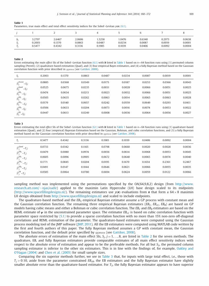
Table 1Parameters, true main effect and total effect sensitivity indices for the Sobol'–Levitan yðxÞ (6.1).

j 1 2 3 4 5 6 7 8

bj 3.2797 2.6467 2.0606 1.5258 1.0476 0.6340 0.2973 0.0638Sj 0.2003 0.1370 0.0863 0.0487 0.0234 0.0087 0.0019 0.0001Tj 0.5477 0.4342 0.3136 0.1985 0.1039 0.0406 0.0092 0.0004

Table 2Errors estimating the main effect SIs of the Sobol'–Levitan function (6.1) with b listed in Table 1 based on n¼64 function runs using (1) permuted columnsampling (PermS); (2) quadrature-based estimation (Quad), and (3) four empirical Bayes estimators, and (4) a fully Bayesian method based on the Gaussiancorrelation function with prior described in gpmsa (see Gattiker, 2008).

Sj 0.2003 0.1370 0.0863 0.0487 0.0234 0.0087 0.0019 0.0001

jbSPermS

j −Sjj 0.0885 0.0368 0.0349 0.0175 0.0187 0.0253 0.0366 0.0043

jbSQuad

j −Sjj 0.0525 0.0675 0.0235 0.0031 0.0028 0.0066 0.0051 0.0025

jbSEBG

j −Sjj 0.0474 0.0634 0.0213 0.0023 0.0032 0.0066 0.0051 0.0025

jbSEBC

j −Sjj 0.0505 0.0635 0.0262 0.0063 0.0014 0.0065 0.0063 0.0028

jbSEBcC

j −Sjj 0.0179 0.0140 0.0657 0.0242 0.0559 0.0649 0.0293 0.0411

jbSEBB

j −Sjj 0.0506 0.0633 0.0204 0.0073 0.0016 0.0074 0.0053 0.0022

jbSFB

j −Sjj 0.0447 0.0613 0.0249 0.0008 0.0036 0.0064 0.0056 0.0027

Table 3Errors estimating the total effect SIs of the Sobol'–Levitan function (6.1) with b listed in Table 1 based on n¼64 function runs using (1) quadrature-basedestimation (Quad), and (2) four (empirical) Bayesian Estimation based on the Gaussian, Bohman, and cubic correlation functions, and (3) a fully Bayesianmethod based on the Gaussian correlation function with prior described in gpmsa (see Gattiker, 2008).

Tj 0.5477 0.4342 0.3136 0.1985 0.1039 0.0406 0.0092 0.0004

jbT Quadj −Tjj 0.0733 0.0342 0.1165 0.0798 0.0660 0.0020 0.0028 0.0036

jbT EBG

j −Tjj 0.0479 0.0080 0.0974 0.0656 0.0614 0.0068 0.0053 0.0045

jbT EBC

j −Tjj 0.0605 0.0096 0.0905 0.0672 0.0640 0.0065 0.0074 0.0040

jbT EBcC

j −Tjj 0.1771 0.0845 0.0204 0.0195 0.1670 0.1654 0.2361 0.2467

jbT EBB

j −Tjj 0.0491 0.0147 0.1044 0.0646 0.0621 0.0066 0.0055 0.0035

jbT FBj −Tjj 0.0585 0.0064 0.0780 0.0694 0.0624 0.0059 0.0122 0.0066

J. Svenson et al. / Journal of Statistical Planning and Inference 144 (2014) 160–172 169

sampling method was implemented using the permutations specified by the OA(64,9,8,2) design (from http://www.research.att.com/�njas/oadir) applied to the maximin Latin Hypercube (LH) base design scaled to its midpoints(http://www.spacefillingdesigns.nl/). The remaining estimators use yðxÞ evaluations from x that form a 64�8 maximinLH design obtained from http://www.spacefillingdesigns.nl/ and scaled to include endpoints.

The quadrature-based method and the EBG empirical Bayesian estimator assume a GP process with constant mean andthe Gaussian correlation function. The remaining three empirical Bayesian estimators (EBC, EBcC, EBB) are based on GPmodels having cubic means and either a Bohman or cubic correlation function. The EBC and EBB estimators are based on theREML estimate of ψ in the unconstrained parameter space. The estimator EBcC is based on cubic correlation function withparameter space restricted by (5.1) to provide a sparse correlation function with no more than 15% non-zero off-diagonalcorrelations and REML estimation of the parameter. The quadrature-based estimates were computed using the Gaussianprocess modeling tool of the JMP software (JMP, 2011). All the EB estimators were computed using MATLAB code written bythe first and fourth authors of this paper. The fully Bayesian method assumes a GP with constant mean, the Gaussiancorrelation function, and the default prior specified by gpmsa (see Gattiker, 2008).

The absolute errors of estimation of the main effect SIs, Sj, j¼ 1;…;8, are listed in Table 2 for the seven methods. Thequadrature, EB, and fully Bayesian estimators provide comparable estimates of all main effect sensitivity indices withrespect to the absolute error of estimation and appear to be the preferable methods. For all but S2, the permuted columnsampling estimator is inferior to the other six estimators. This is in line with the findings of, for example, Oakley andO’Hagan (2004) and Chen et al. (2005) for small sample sizes.

Comparing the six superior methods further, we see in Table 3 that, for inputs with large total effect, i.e., those withTj40:10, aside from the parameter constrained EBcB, the EB estimators and the fully Bayesian estimator have slightlysmaller absolute error than the quadrature-based estimator. For T2, the fully Bayesian estimator appears to have superior

J. Svenson et al. / Journal of Statistical Planning and Inference 144 (2014) 160–172170

performance. We increased the percentage of non-zero non-diagonal correlation elements to 50% to allow more data in theprediction process. The errors of estimation of the total effect SIs remained substantially larger than those of the other EBestimators. Of course allowing all the data to be used in the estimation of ψ as for EBB or EBC does produce reasonable SIestimates. EB estimation based on a constrained parameter space suffers from the same type of estimation errors as doesEBcB. In sum, when the amount of data used to estimate the model parameters is too “small”, the EB estimators of the SIs canbe severely negatively impacted.

We increased the number of function evaluations to 81, using the orthogonal array OAð81;10;9;2Þ from the websiteabove for the permuted column sampling. All methods provided better estimates, but the relative performance remainedthe same. Consequently, it appears that, on the whole, the Bayesian methodology preforms slightly better than the othertwo methods for estimation of main effect and total effect sensitivity indices.

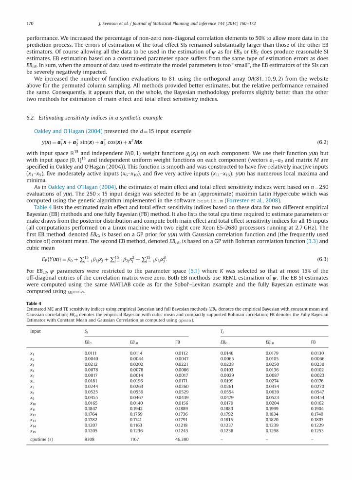
6.2. Estimating sensitivity indices in a synthetic example

Oakley and O’Hagan (2004) presented the d¼15 input example

yðxÞ ¼ a⊤1xþ a⊤

2 sinðxÞ þ a⊤3 cosðxÞ þ x⊤Mx ð6:2Þ

with input space R15 and independent Nð0;1Þ weight functions gjðxjÞ on each component. We use their function yðxÞ butwith input space ½0;1�15 and independent uniform weight functions on each component (vectors a1–a3 and matrix M arespecified in Oakley and O'Hagan (2004)). This function is smooth and was constructed to have five relatively inactive inputs(x1–x5), five moderately active inputs (x6–x10), and five very active inputs (x11–x15); yðxÞ has numerous local maxima andminima.

As in Oakley and O’Hagan (2004), the estimates of main effect and total effect sensitivity indices were based on n¼250evaluations of yðxÞ. The 250�15 input design was selected to be an (approximate) maximin Latin Hypercube which wascomputed using the genetic algorithm implemented in the software bestlh.m (Forrester et al., 2008).

Table 4 lists the estimated main effect and total effect sensitivity indices based on these data for two different empiricalBayesian (EB) methods and one fully Bayesian (FB) method. It also lists the total cpu time required to estimate parameters ormake draws from the posterior distribution and compute both main effect and total effect sensitivity indices for all 15 inputs(all computations performed on a Linux machine with two eight core Xeon E5-2680 processors running at 2.7 GHz). Thefirst EB method, denoted EBG, is based on a GP prior for yðxÞ with Gaussian correlation function and (the frequently usedchoice of) constant mean. The second EB method, denoted EBcB, is based on a GP with Bohman correlation function (3.3) andcubic mean

EPfYðxÞg ¼ β0 þ∑15j ¼ 1β1jxj þ∑15

j ¼ 1β2jx2j þ∑15

j ¼ 1β3jx3j : ð6:3Þ

For EBcB, ψ parameters were restricted to the parameter space (5.1) where K was selected so that at most 15% of theoff-diagonal entries of the correlation matrix were zero. Both EB methods use REML estimation of ψ . The EB SI estimateswere computed using the same MATLAB code as for the Sobol'–Levitan example and the fully Bayesian estimate wascomputed using gpmsa.

Table 4Estimated ME and TE sensitivity indices using empirical Bayesian and full Bayesian methods (EBG denotes the empirical Bayesian with constant mean andGaussian correlation; EBcB denotes the empirical Bayesian with cubic mean and compactly supported Bohman correlation; FB denotes the Fully BayesianEstimator with Constant Mean and Gaussian Correlation as computed using gpmsa).

Input Sj Tj

EBG EBcB FB EBG EBcB FB

x1 0.0111 0.0114 0.0112 0.0146 0.0179 0.0130x2 0.0040 0.0044 0.0047 0.0065 0.0105 0.0066x3 0.0212 0.0202 0.0221 0.0228 0.0250 0.0230x4 0.0078 0.0078 0.0086 0.0103 0.0136 0.0102x5 0.0017 0.0014 0.0017 0.0029 0.0087 0.0023x6 0.0181 0.0196 0.0171 0.0199 0.0274 0.0176x7 0.0244 0.0263 0.0260 0.0261 0.0334 0.0270x8 0.0525 0.0559 0.0529 0.0554 0.0639 0.0547x9 0.0455 0.0467 0.0439 0.0479 0.0523 0.0454x10 0.0165 0.0140 0.0156 0.0179 0.0204 0.0162x11 0.1847 0.1942 0.1889 0.1883 0.1999 0.1904x12 0.1764 0.1759 0.1736 0.1792 0.1834 0.1740x13 0.1782 0.1741 0.1791 0.1815 0.1820 0.1803x14 0.1207 0.1163 0.1218 0.1237 0.1239 0.1229x15 0.1205 0.1236 0.1243 0.1238 0.1298 0.1253

cputime (s) 9308 1167 46,380 – – –

J. Svenson et al. / Journal of Statistical Planning and Inference 144 (2014) 160–172 171

For this smooth function, n¼250 observations are more than sufficient to provide a good overall estimate (see Loeppkyet al., 2009). The results listed in Table 4 show that all three methods provide comparable estimates of both the main effectand total effect sensitivity indices. However, the methods are distinguished by the times required to produce theseestimates. The EBcB method with sparse correlation matrix required only 1167 s of cpu time to produce estimates similar tothose given by the EBG estimator while the latter required over 9000 s of cpu time. This example provides anotherillustration suggesting that, even with a more complicated fitted mean, the GP model with a sparse correlation matrixinduced by the Bohman correlation, can be used to estimate and predict in cases of larger n than is possible with theGaussian correlation function with constant mean (see Kaufman et al., 2011). In fact, an additional SI estimation based on GPwith Gaussian correlation function model but with a cubic mean (6.3) (not shown) required 12,926 s of cpu time (andresulted in essentially equivalent numerical SI estimates). The fully Bayesian FB method required much longer, 46,380 s ofcpu time, than either EB method to estimate the SIs; of this computational time, 41,167 s were used to construct 10,000posterior draws of the parameters and an additional 5213 s to evaluate the SI formulas for the 500 equally spaced posteriordraws selected from the 10,000 generated. We conclude by noting that estimates of the SIs based on a GP with cubiccorrelation and cubic mean produced similar numerical estimates to those shown in Table 4 and required 1139 s of cpu time,a value comparable to the Bohman-based estimates. In sum, this example provides additional evidence of the value of usingcompactly supported correlation functions when the amount of the data is “large.”

7. Summary and discussion

This paper presents estimation formulae for quadrature-based, Bayesian, and empirical Bayesian estimators of maineffect and total effect sensitivity indices. The Bayesian estimator is a posterior mean of the variance of an averaged outputvalue using a Gaussian process prior for the output function. Specific estimation formulae are given for a broad class ofregression plus stationary Gaussian process prior models that are based on the Gaussian, Bohman or cubic correlationfunctions. For small n/d, all methods yield numerically similar estimates. For larger n/d, estimators based on compactlysupported Bohman and cubic correlation functions (when used with non-constant regression means) can provide significantcpu savings when the correlation matrix is constrained to be sparse and they are numerically similar to sensitivity indexestimates based on non-compactly supported correlation functions. To facilitate the use of sparse correlation structures, weprovide a method determining the parameter space that controls the degree of sparsity for the Bohman and cubiccorrelation functions.

Acknowledgments

This research was sponsored, in part, by the National Science Foundation under Agreement DMS-0806134 (The OhioState University). This paper was completed at the Isaac Newton Institute for the Mathematical Sciences during the 2011Programme on the Design and Analysis of Experiments. The authors would like to thank the referees for their helpfulcomments which have led to a considerably improved paper, and to thank Fangfang Sun for help with the some of thecomputations used in the paper.

Appendix A. Supplementary data

Supplementary data associated with this article can be found in the online version at http://dx.doi.org.10.1016/j.jspi.2013.04.003.

References

Barry, R.P., Pace, R.K., 1997. Kriging with large data sets using sparse matrix techniques. Communications in Statistics—Simulation and Computation 26,619–629.

Campolongo, F., Cariboni, J., Saltelli, A., 2007. An effective screening design for sensitivity analysis of large models. Environmental Modelling & Software 22,1509–1518.

Chen, W., Jin, R., Sudjianto, A., 2005. Analytical variance-based global sensitivity analysis in simulation-based design under uncertainty. Journal ofMechanical Design 127, 875–876.

Chen, W., Jin, R., Sudjianto, A., 2006. Analytical global sensitivity analysis and uncertainty propogation for robust design. Journal of Quality Technology 38,333–348.

Currin, C., Mitchell, T.J., Morris, M.D., Ylvisaker, D., 1991. Bayesian prediction of deterministic functions, with applications to the design and analysis ofcomputer experiments. Journal of the American Statistical Association 86, 953–963.

Da Viega, S., Wahl, F., Gamboa, F., 2009. Local polynomial estimation for sensitivity analysis on models with correlated inputs. Technometrics 51, 452–463.Forrester, A., Sobester, A., Keane, A., 2008. Engineering Design via Surrogate Modelling: A Practical Guide. Wiley, Chichester, UK.Gattiker, J.R., 2008. Gaussian Process Models for Simulation Analysis (GPM/SA) Command, Function, and Data Structure Reference. Technical Report LA-UR-

08-08057, Los Alamos National Laboratory.Gilbert, J.R., Moler, C., Schreiber, R., 1991. Sparse Matrices in MATLAB: Design and Implementation. SIAM Journal on Matrix Analysis and Applications 13,

333–356.Helton, J.C., Johnson, J.D., Sallaberry, C.J., Storlie, C.B., 2006. Survey of sampling-based methods for uncertainty and sensitivity analysis. Reliability

Engineering and System Safety 91, 1175–1209.

J. Svenson et al. / Journal of Statistical Planning and Inference 144 (2014) 160–172172

Higdon, D., Gattiker, J., Williams, B., Rightley, M., 2008. Computer model calibration using high dimensional output. Journal of the American StatisticalAssociation 103, 570–583.

Homma, T., Saltelli, A., 1996. Importance measures in global sensitivity analysis of model output. Reliability Engineering and System Safety 52, 1–17.JMP, 2011. Version 9.Jones, D.R., Schonlau, M., Welch, W.J., 1998. Efficient global optimization of expensive black-box functions. Journal of Global Optimization 13, 455–492.Kaufman, C., Bingham, D., Habib, S., Heitmann, K., Frieman, J., 2011. Efficient emulators of computer experiments using compactly supported correlation

functions, with an application to cosmology. The Annals of Applied Statistics 5, 2470–2492.Linkletter, C., Bingham, D., Hengartner, N., Higdon, D., Ye, K.Q., 2006. Variable selection for Gaussian process models in computer experiments.

Technometrics 48, 478–490.Loeppky, J.L., Sacks, J., Welch, W.J., 2009. Choosing the sample size of a computer experiment: a practical guide. Technometrics 51, 366–376.Marrel, A., Iooss, B., Lauren, B., Roustant, O., 2009. Calculations of Sobol indices for the Gaussian process metamodel. Reliability Engineering and System

Safety 94, 742–751.Moon, H., Santner, T.J., Dean, A.M., 2012. Two-stage sensitivity-based group screening in computer experiments. Technometrics 54, 376–387.Morris, M.D., 1991. Factorial sampling plans for preliminary computational experiments. Technometrics 33, 161–174.Morris, M.D., Moore, L.M., McKay, M.D., 2008. Using orthogonal arrays in the sensitivity analysis of computer models. Technometrics 50, 205–215.Oakley, J.E., O’Hagan, A., 2004. Probabilistic sensitivity analysis of complex models: a Bayesian approach. Journal of the Royal Statistical Society B 66,

751–769.O'Hagan, A., 1992. Some Bayesian numerical analysis. In: Bernardo, J.M., Berger, J.O., Dawid, A.P., Smith, A.F.M. (Eds.), Bayesian Statistics, vol. 4. . Oxford

University Press, pp. 345–363.Sacks, J., Schiller, S.B., Welch, W.J., 1989a. Design for computer experiments. Technometrics 31, 41–47.Sacks, J., Welch, W.J., Mitchell, T.J., Wynn, H.P., 1989b. Design and analysis of computer experiments. Statistical Science 4, 409–423.Saltelli, A., 2002. Making best use of model evaluations to compute sensitivity indices. Computer Physics Communications 145 (2), 280–297.Saltelli, A., Annoni, P., Azzini, I., Campolongo, F., Ratto, M., Tarantola, S., 2010. Variance based sensitivity analysis of model output. Design and estimator for

the total sensitivity index. Computer Physics Communications 181, 259–270.Saltelli, A., Tarantola, S., Campolongo, F., 2000. Sensitivity analysis as an ingredient of modeling. Statistical Science 15, 377–395.Santner, T.J., Williams, B.J., Notz, W.I., 2003. The Design and Analysis of Computer Experiments. Springer Verlag, New York.Sobol', I., Levitan, Y., 1999. On the use of variance reducing multipliers in Monte Carlo computations of a global sensitivity index. Computer Physics

Communications 117, 52–61.Sobol', I.M., 1990. Sensitivity estimates for non-linear mathematical models. Matematicheskoe Modelirovanie 2, 112–118.Sobol', I.M., 1993. Sensitivity analysis for non-linear mathematical models. Mathematical Modeling and Computational Experiment 1, 407–414.Storlie, C.B., Reich, B.J., Helton, J.C., Swiler, L.P., Sallaberry, C.J., 2013. Analysis of computationally demanding models with continuous and categorical inputs.

Reliability Engineering and System Safety 113, 30–41.Van Der Vaart, A.W., 1998. Asymptotic Statistics Cambridge. University Press, Cambridge, UK.Welch, W.J., Buck, R.J., Sacks, J., Wynn, H.P., Mitchell, T.J., Morris, M.D., 1992. Screening, predicting, and computer experiments. Technometrics 34, 15–25.