CONTRIBUTED RESEARCH ARTICLES 130

Estimating Spatial Probit Models in Rby Stefan Wilhelm and Miguel Godinho de Matos

Abstract In this article we present the Bayesian estimation of spatial probit models in R and provide animplementation in the package spatialprobit. We show that large probit models can be estimated withsparse matrix representations and Gibbs sampling of a truncated multivariate normal distribution withthe precision matrix. We present three examples and point to ways to achieve further performancegains through parallelization of the Markov Chain Monte Carlo approach.

Introduction

The abundance of geolocation data and social network data has lead to a growing interest in spatialeconometric methods, which model a contemporaneous dependence structure using neighboringobservations (e.g. friends in social networks).

There are a variety of R packages for spatial models available, an incomplete list includes spBayes(Finley and Banerjee, 2013), spatial (Venables and Ripley, 2002), geostatistical packages called geoR(Diggle and Ribeiro, 2007) and sgeostat (Majure and Gebhardt, 2013), spdep (Bivand, 2013), sphet(Piras, 2010), sna (Butts, 2013) and network (Butts et al., 2013).

While all of these packages deal with linear spatial models, in this article we focus on a nonlinearmodel, the spatial probit model, and present the Bayesian estimation first proposed by LeSage (2000).As will be shown below, one crucial point we have been working on was the generation of randomnumbers of a truncated multivariate normal distribution in very high dimensions.

Together with these high dimensions and the size of problems in spatial models comes the need towork with sparse matrix representations rather than the usual dense matrix(). Popular R packagesfor dealing with sparse matrices are Matrix (Bates and Maechler, 2013) and sparseM (Koenker andNg, 2013).

In the next section we first introduce spatial probit models and describe the Bayesian estimationprocedure of the SAR probit model in detail. Subsequently we discuss some implementation issues inR, describe the sarprobit method in package spatialprobit (Wilhelm and de Matos, 2013), compareit against maximum likelihood (ML) and generalized method of moments (GMM) estimation inMcSpatial (McMillen, 2013) and illustrate the estimation with an example from social networks. Wealso illustrate how to parallelize the Bayesian estimation with the parallel package.

Spatial probit models

The book of LeSage and Pace (2009) is a good starting point and reference for spatial econometricmodels in general and for limited dependent variable spatial models in particular (chapter 10, p. 279).

Suppose we have the spatial autoregressive model (SAR model, spatial lag model)

z = ρWz + Xβ + ε, ε ∼ N(

0, σ2ε In

)(1)

for z = (z1, . . . , zn)′ with some fixed matrix of covariates X (n× k) associated with the parametervector β (k× 1). The matrix W (n× n) is called the spatial weight matrix and captures the dependencestructure between neighboring observations such as friends or nearby locations. The term Wz is alinear combination of neighboring observations. The scalar ρ is the dependence parameter and willassumed abs(ρ) < 1. The k + 1 model parameters to be estimated are the parameter vector β and thescalar ρ.

In a spatial probit model, z is regarded as a latent variable, which cannot be observed. Instead, theobservables are only binary variables yi (0, 1) as

yi =

{1 if zi ≥ 0,0 if zi < 0.

yi can reflect any binary outcome such as survival, a buy/don’t buy decision or a class variable inbinary classification problems. For identification, σ2

ε is often set to σ2ε = 1.

The R Journal Vol. 5/1, June 2013 ISSN 2073-4859

CONTRIBUTED RESEARCH ARTICLES 131

The data generating process for z is

z = (In − ρW)−1 Xβ + (In − ρW)−1 ε

ε ∼ N (0, In)

Note that if ρ = 0 or W = In, the model reduces to an ordinary probit model, for which Wooldridge(2002, chapter 17) and Albert (2007, section 10.1) are good references. The ordinary probit model canbe estimated in R by glm().

Another popular spatial model is the spatial error model (SEM) which takes the form

z = Xβ + u, u = ρWu + ε, ε ∼ N(

0, σ2ε In

)(2)

z = Xβ + (In − ρW)−1 ε

where as before, only binary variables yi (0,1) can be observed instead of zi. Our following discussionfocuses on the spatial lag probit model (1), but the estimation of the probit model with spatial errors iscovered in spatialprobit as well.

Recent studies using spatial probit models include, among others, Marsh et al. (2000), Klier andMcMillen (2008) and LeSage et al. (2011).

Bayesian estimation

Maximum Likelihood and GMM estimation of the spatial probit is implemented in the packageMcSpatial (McMillen, 2013) with the methods spprobitml and spprobit. Here we present the detailsof Bayesian estimation. Although GMM is massively more efficient computationally than BayesianMarkov Chain Monte Carlo (MCMC), as a instrumental-variables estimation it will work well only invery large samples. This point is also brought by Franzese et al. (2013), who compares different spatialprobit estimation strategies.

The basic idea in Bayesian estimation is to sample from a posterior distribution of the modelparameters p(z, β, ρ|y) given the data y and some prior distributions p(z), p(β), p(ρ). See for exampleAlbert (2007) and the accompanying package LearnBayes for an introduction to Bayesian statisticsin R (Albert, 2012). This sampling for the posterior distribution p(z, β, ρ|y) can be realized by aMarkov Chain Monte Carlo and Gibbs sampling scheme, where we sample from the following threeconditional densities p(z|β, ρ, y), p(β|z, ρ, y) and p(ρ|z, β, y):

1. Given the observed variables y and parameters β and ρ, we have p(z|β, ρ, y) as a truncatedmultinormal distribution

z ∼ N((In − ρW)−1 Xβ,

[(In − ρW)′ (In − ρW)

]−1)

(3)

subject to zi ≥ 0 for yi = 1 and zi < 0 for yi = 0, which can be efficiently sampled from usingthe method rtmvnorm.sparseMatrix() in package tmvtnorm (Wilhelm and Manjunath, 2013),see the next section for details.

2. For a normal prior β ∼ N(c, T), we can sample p(β|ρ, z, y) from a multivariate normal as

p (β|ρ, z, y) ∝ N (c∗, T∗) (4)

c∗ =(

X′X + T−1)−1 (

X′Sz + T−1c)

T∗ =(

X′X + T−1)−1

S = (In − ρW)

The standard way for sampling from this distribution is rmvnorm() from package mvtnorm(Genz et al., 2013).

3. The remaining conditional density p(ρ|β, z, y) is

p (ρ|β, z, y) ∝ |In − ρW| exp(−1

2(Sz− Xβ)′ (Sz− Xβ)

)(5)

which can be sampled from using Metropolis-Hastings or some other sampling scheme (i.e.Importance Sampling). We implement a grid-based evaluation and numerical integrationproposed by LeSage and Pace and then draw from the inverse distribution function (LeSageand Pace, 2009, p. 132).

The R Journal Vol. 5/1, June 2013 ISSN 2073-4859

CONTRIBUTED RESEARCH ARTICLES 132

Implementation issues

Since MCMC methods are widely considered to be (very) slow, we devote this section to the discussionof some implementation issues in R. Key factors to estimate large spatial probit models in R include theusage of sparse matrices and compiled Fortran code, and possibly also parallelization, which has beenintroduced to R 2.14.0 with the package parallel. We report estimation times and memory requirementsfor several medium-size and large-size problems and compare our times to those reported by LeSageand Pace (2009, p. 291). We show that our approach allows the estimation of large spatial probit modelsin R within reasonable time.

Drawing p(z|β, ρ, y)

In this section we describe the efforts made to generate samples from p(z|β, ρ, y)

z ∼ N((In − ρW)−1 Xβ,

[(In − ρW)′ (In − ρW)

]−1)

subject to zi ≥ 0 for yi = 1 and zi < 0 for yi = 0.

The generation of samples from a truncated multivariate normal distribution in high dimensionsis typically done with a Gibbs sampler rather than with other techniques such as rejection sampling(for a comparison, see Wilhelm and Manjunath (2010)). The Gibbs sampler draws from univariateconditional densities f (zi|z−i) = f (zi|z1, . . . , zi−1, zi+1, . . . , zn).

The distribution of zi conditional on z−i is univariate truncated normal with variance

Σi.−i = Σii − Σi,−iΣ−1−i,−iΣ−i,i (6)

= H−1ii (7)

and mean

µi.−i = µi + Σi,−iΣ−1−i,−i

(z−i − µ−i

)(8)

= µi −H−1ii Hi,−i

(z−i − µ−i

)(9)

and bounds −∞ ≤ zi ≤ 0 for yi = 0 and 0 ≤ zi ≤ ∞ for yi = 1.

Package tmvtnorm has such a Gibbs sampler in place since version 0.9, based on the covariancematrix Σ. Following Geweke (1991, 2005, p. 171), the Gibbs sampler is easier to state in terms of theprecision matrix H, simply because it requires fewer and easier operations in the above equations (7)and (9). These equations will further simplify in the case of a sparse precision matrix H, in which mostof the elements are zero. With sparse H, operations involving Hi,−i need only to be executed for allnon-zero elements rather than for all n− 1 variables in z−i.

In our spatial probit model, the covariance matrix Σ = [(In − ρW)′(In − ρW)]−1 is a dense matrix,whereas the corresponding precision matrix H = Σ−1 = (In − ρW)′(In − ρW) is sparse. Hence, usingΣ for sampling z is inefficient. For this reason we reimplemented the Gibbs sampler with the precisionmatrix H in package tmvtnorm instead (Wilhelm and Manjunath, 2013).

Suppose one wants to draw N truncated multinormal samples in n dimensions, where the precisionmatrix H is sparse (n× n) with only m < n entries different from zero per row on average (e.g. m = 6nearest neighbors or average branching factor in a network). With growing dimension n, two types ofproblems arise with a usual dense matrix representation for H:

1. Data storage problem: Since matrix H is n× n, the space required to store the dense matrixwill be quadratic in n. One remedy is, of course, using some sparse matrix representation for H(e.g. packages Matrix, sparseM etc.), which actually holds only n ·m elements instead of n · n.The following code example shows the difference in object sizes for a dense vs. sparse identitymatrix In for n = 10000 and m = 1.

> library(Matrix)> I_n_dense <- diag(10000)> print(object.size(I_n_dense), units = "Mb")

762.9 Mb

> rm(I_n_dense)> I_n_sparse <- sparseMatrix(i = 1:10000, j = 1:10000, x = 1)> print(object.size(I_n_sparse), units = "Mb")

0.2 Mb

The R Journal Vol. 5/1, June 2013 ISSN 2073-4859

CONTRIBUTED RESEARCH ARTICLES 133

2. Data access problem: Even with a sparse matrix representation for H, a naive strategy that triesto access an arbitrary matrix element H[i,j] like in triplet or hash table representations, willresult in N · n · n matrix accesses to H. This number grows quadratically in n. For example, forN = 30 and n = 10000 it adds up to 30 · 10000 · 10000 = 3 billion hash function calls, which isinefficient and too slow for most applications.Iterating only over the non-zero elements in row i, for example in term Hi,−i, reduces the numberof accesses to H to only N · n ·m instead of N · n · n, which furthermore will only grow linearlyin n for a fixed m. Suitable data structures to access all non-zero elements of the precision matrixH are linked lists of elements for each row i (list-of-lists) or, thanks to the symmetry of H, thecompressed-sparse-column/row representation of sparse matrices, directly available from theMatrix package.

How fast is the random number generation for z now? We performed a series of tests for varyingsizes N and n and two different values of m. The results presented in Table 1 show that the samplerwith sparse H is indeed very fast and works fine in high dimensions. The time required scales withN · n.

Nn 101 102 103 104 105 106

m=2 101 0.03 0.25 2.60102 0.03 0.25 2.75103 0.03 0.25 2.84104 0.03 0.25 2.80105 0.26 2.79

m=6 101 0.03 0.23 2.48102 0.01 0.23 2.53103 0.03 0.23 2.59104 0.02 0.24 2.57105 0.25 2.68

Table 1: Performance test results for the generation of truncated multivariate normal samples z withrtmvnorm.sparseMatrix() (tmvtnorm) for a varying number of samples N and dimension n. Theprecision matrix in each case is H = (In − ρW)′(In − ρW), the spatial weight matrix W contains mnon-zero entries per row. Times are in seconds and measured on an Intel® Core™i7-2600 CPU @3.40GHz.

One more performance issue we discuss here is the burn-in size in the innermost Gibbs samplergenerating z from p(z|β, ρ, y). Depending on the start value, Gibbs samplers often require a certainburn-in phase until the sampler mixes well and draws from the desired target distribution. In ourMCMC setup, we only draw one sample of z from p(z|β, ρ, y) in each MCMC iteration, but possiblyin very high dimensions (e.g. N = 1, n = 10000). With burn.in=20 samples, we have to generate 21draws in order to keep just one. In our situation, a large burn-in size will dramatically degrade theMCMC performance, so the number of burn-in samples for generating z has to be chosen carefully.LeSage and Pace (2009) discuss the role of the burn-in size and often use burn.in=10, when theGibbs sampler starts from zero. Alternatively, they also propose to use no burn-in phase at all (e.g.burn.in=0), but then to set the start value of the sampler to the previous value of z instead of zero.

QR decomposition of (In − ρW)

The mean vector µ of the truncated normal samples z in equation (3) takes the form

µ = (In − ρW)−1 Xβ (10)

However, inverting the sparse matrix S = (In − ρW) will produce a dense matrix and will thereforeoffset all benefits from using sparse matrices (i.e. memory consumption and size of problems thatcan be solved). It is preferable to determine µ by solving the equations (In − ρW)µ = Xβ with a QRdecomposition of S = (In − ρW). We point out that there is a significant performance differencebetween the usual code mu <-qr.solve(S,X %*% beta) and mu <-solve(qr(S),X %*% beta). Thelatter will apply a QR decomposition for a sparse matrix S and will use a method qr() from thepackage Matrix, whereas the first function from the base package will coerce S into a dense matrix.

The R Journal Vol. 5/1, June 2013 ISSN 2073-4859

CONTRIBUTED RESEARCH ARTICLES 134

solve(qr(S),X %*% beta) takes only half the time required by qr.solve(S,X %*% beta).

Drawing p(β|z, ρ, y)

Drawing p(β|z, ρ, y) in equation (4) is a multivariate normal distribution, whose variance T∗ doesnot depend on z and ρ. Therefore, we can efficiently vectorize and generate temporary drawsβtmp ∼ N(0, T∗) for all MCMC iterations before running the chain and then just shift these temporarydraws by c∗ in every iteration to obtain a β ∼ N(c∗, T∗).

Determining log-determinants and drawing p(ρ|z, β, y)

The computation of log-determinants for ln |In − ρW|, whose evaluation is frequently needed fordrawing p(ρ|z, β, y), becomes a challenging task for large matrices. Bivand (2010) gives a survey of thedifferent methods for calculating the Jacobian like the Pace and Barry (1997) grid evaluation of ρ in theinterval [−1, . . . ,+1] and spline approximations between grid points or the Chebyshev approximationof the log-determinant (Pace and LeSage, 2004). All of them are implemented in package spdep. Forthe estimation of the probit models we are using the existing facilities in spdep (do_ldet()).

Computation of marginal effects

In spatial lag models (and its probit variants), a change of an explanatory variable xir will affectboth the same response variable zi (direct effects) and possibly all other responses zj (j 6= i; indirecteffects or spatial spillovers). The resulting effects matrix Sr(W) is n× n for xr (r = 1, . . . , k) and threesummary measures of Sr(W) will be computed: average direct effects (Mr(D) = n−1trSr(W)), averagetotal effects (Mr(T) = n−11′nSr(W)1n) and the average indirect effects as the difference of total anddirect effects (Mr(I) = Mr(T)−Mr(D)). In contrast to the SAR probit, there are no spatial spill-overeffects in the SEM probit model (2). In the MATLAB spatial econometrics toolbox (LeSage, 2010), thecomputation of the average total effects requires an inversion of the n× n matrix S = (In − ρW) atevery MCMC iteration. Using the same QR-decomposition of S as described above and solving theequation solve(qr(S),rep(1,n)) speeds up the calculation of total effects by magnitudes.

Examples

Package spatialprobit

After describing the implementation issues to ensure that the estimation is fast enough and capableto handle large problems, we briefly describe the interface of the methods in package spatialprobit(Wilhelm and de Matos, 2013) and then turn to some examples.

The main estimation method for the SAR probit model sar_probit_mcmc(y,X,W) takes a vector ofdependent variables y, a model matrix X and a spatial weight matrix W. The method sarprobit(formula,W,data) is a wrapper which allows a model formula and a data frame. Both methods require a spatialweight matrix W to be passed as an argument. Additionally, the number of MCMC start values,the number of burn-in iterations and a thinning parameter can be specified. The estimation fit<-sarprobit(y ~ x,W,data) returns an object of class sarprobit. The model coefficients can beextracted via coef(fit). summary(fit) returns a coefficient table with z-values, impacts(fit) givesthe marginal effects and the plot(fit) method provides MCMC trace plots, posterior density plotsas well as autocorrelation plots of the model parameters. logLik(fit) and AIC(fit) return the loglikelihood and the AIC of the model for model comparison and testing.

Experiment from LeSage/Pace

We replicate the experiment from LeSage and Pace (2009, section 10.1.5) for n = 400 and n = 1000random points in a plane and a spatial weight matrix with the 6 nearest neighbors. The spatial probitmodel parameters are σ2

ε = 1, β = (0, 1,−1)′ and ρ = 0.75. We generate data from this model with thefollowing code.

> library(spatialprobit)> set.seed(2)> n <- 400> beta <- c(0, 1, -1)> rho <- 0.75

The R Journal Vol. 5/1, June 2013 ISSN 2073-4859

CONTRIBUTED RESEARCH ARTICLES 135

> X <- cbind(intercept = 1, x = rnorm(n), y = rnorm(n))> I_n <- sparseMatrix(i = 1:n, j = 1:n, x = 1)> nb <- knn2nb(knearneigh(cbind(x = rnorm(n), y = rnorm(n)), k = 6))> listw <- nb2listw(nb, style = "W")> W <- as(as_dgRMatrix_listw(listw), "CsparseMatrix")> eps <- rnorm(n = n, mean = 0, sd = 1)> z <- solve(qr(I_n - rho * W), X %*% beta + eps)> y <- as.double(z >= 0)

We estimate the spatial probit model as

> sarprobit.fit1 <- sarprobit(y ~ X - 1, W, ndraw = 1000, burn.in = 200,+ thinning = 1, m = 10)> summary(sarprobit.fit1)> plot(sarprobit.fit1)

Table 2 shows the results of the SAR probit estimation for the same experiment as in LeSage andPace (2009). The results shown there can be replicated either using the code above (for n = 400) orusing the LeSagePaceExperiment() function in the package and setting set.seed(2) (for n = 400 andn = 1000)):

> set.seed(2)> res1 <- LeSagePaceExperiment(n = 400, beta = c(0, 1, -1), rho = 0.75,+ ndraw = 1000, burn.in = 200, thinning = 1, m = 10)> summary(res1)> set.seed(2)> res2 <- LeSagePaceExperiment(n = 1000, beta = c(0, 1, -1), rho = 0.75,+ ndraw = 1000, burn.in = 200, thinning = 1, m = 1)> summary(res2)

The corresponding ML and GMM estimates in Table 2 can be replicated by creating the data as above(replacing n <-1000 for n = 1000 accordingly) and

> library(McSpatial)> wmat <- as.matrix(W)> mle.fit1 <- spprobitml(y ~ X[, "x"] + X[, "y"], wmat = wmat)> gmm.fit1 <- spprobit(y ~ X[, "x"] + X[, "y"], wmat = wmat)

Our Bayesian estimation yields similar results, but our implementation is much faster (factor20-100) than the LeSage implementation, even on a single core. The McSpatial GMM estimation seemsto be biased in this example. The evaluation of the performance relative to McSpatial ML clearlyneeds to take into account a number of factors: First, the choice of the number of MCMC iterations Nand burn.in samples, as well as m do control the estimation time to a large degree. Second, the currentML implementation in McSpatial does not compute marginal effects. Finally, McSpatial works withdense matrices which is superior for smaller sample sizes, but will not scale for larger n.

Table 3 shows that a change of the Gibbs sampler burn-in size m for drawing z has little effect onthe mean and the variance of the estimates. m = 1 means taking the previous value of z, m = 2, 5, 10start the chain from z = 0. Clearly, choosing m = 2 might not be enough as burn-in phase.

Random graph example

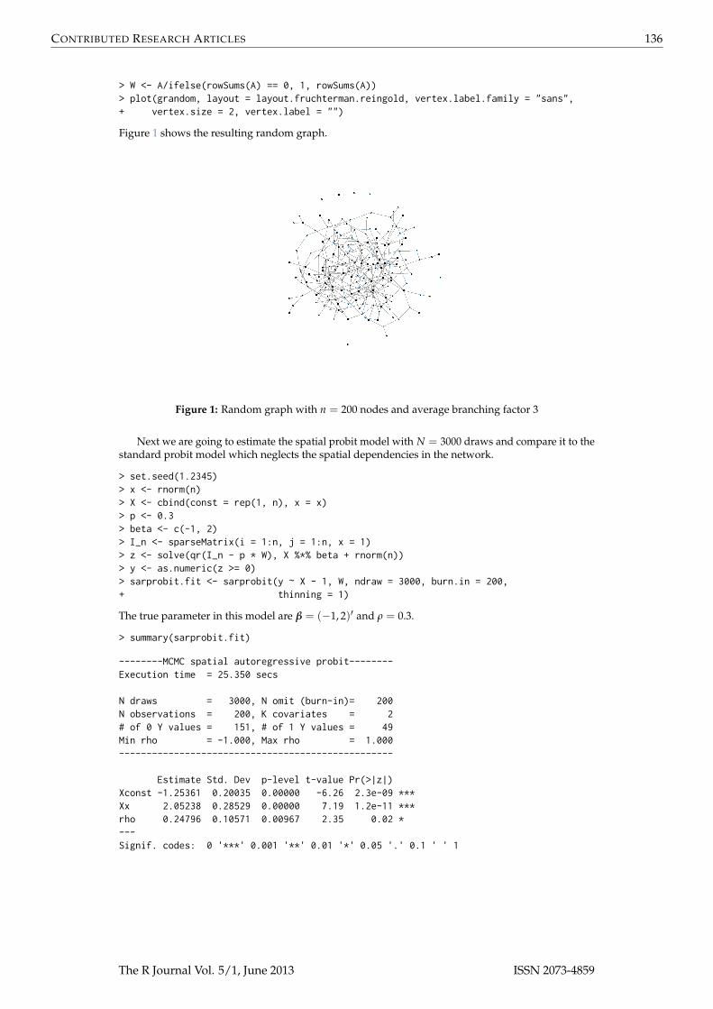
As a second example we present the estimation of the probit model based on a random undirectedgraph with n = 200 nodes and an average branching factor of 3. Of course this estimation procedurecan be applied to real network structures such as from social networks. The package igraph can beused to create random graphs and to compute the adjacency matrix A as well as the spatial weightmatrix W (Csardi and Nepusz, 2006).

> library(igraph)> library(spatialprobit)> set.seed(1)> n <- 200> branch <- 3> probability <- branch/n> grandom <- igraph::erdos.renyi.game(n = n, p.or.m = probability,+ type = "gnp", directed = F, loops = F)> V(grandom)$name <- 1:n> A <- igraph::get.adjacency(grandom, type = "both", sparse = TRUE)

The R Journal Vol. 5/1, June 2013 ISSN 2073-4859

CONTRIBUTED RESEARCH ARTICLES 136

> W <- A/ifelse(rowSums(A) == 0, 1, rowSums(A))> plot(grandom, layout = layout.fruchterman.reingold, vertex.label.family = "sans",+ vertex.size = 2, vertex.label = "")

Figure 1 shows the resulting random graph.

Figure 1: Random graph with n = 200 nodes and average branching factor 3

Next we are going to estimate the spatial probit model with N = 3000 draws and compare it to thestandard probit model which neglects the spatial dependencies in the network.

> set.seed(1.2345)> x <- rnorm(n)> X <- cbind(const = rep(1, n), x = x)> p <- 0.3> beta <- c(-1, 2)> I_n <- sparseMatrix(i = 1:n, j = 1:n, x = 1)> z <- solve(qr(I_n - p * W), X %*% beta + rnorm(n))> y <- as.numeric(z >= 0)> sarprobit.fit <- sarprobit(y ~ X - 1, W, ndraw = 3000, burn.in = 200,+ thinning = 1)

The true parameter in this model are β = (−1, 2)′ and ρ = 0.3.

> summary(sarprobit.fit)

--------MCMC spatial autoregressive probit--------Execution time = 25.350 secs

N draws = 3000, N omit (burn-in)= 200N observations = 200, K covariates = 2# of 0 Y values = 151, # of 1 Y values = 49Min rho = -1.000, Max rho = 1.000--------------------------------------------------

Estimate Std. Dev p-level t-value Pr(>|z|)Xconst -1.25361 0.20035 0.00000 -6.26 2.3e-09 ***Xx 2.05238 0.28529 0.00000 7.19 1.2e-11 ***rho 0.24796 0.10571 0.00967 2.35 0.02 *---Signif. codes: 0 '***' 0.001 '**' 0.01 '*' 0.05 '.' 0.1 ' ' 1

The R Journal Vol. 5/1, June 2013 ISSN 2073-4859

CONTRIBUTED RESEARCH ARTICLES 137

The direct, indirect and total marginal effects are extracted using

> impacts(sarprobit.fit)

--------Marginal Effects--------

(a) Direct effectslower_005 posterior_mean upper_095

Xx 0.231 0.268 0.3

(b) Indirect effectslower_005 posterior_mean upper_095

Xx -0.299 -0.266 -0.23

(c) Total effectslower_005 posterior_mean upper_095

Xx 0.00149 0.00179 0

The corresponding non-spatial probit model is estimated using the glm() function:

> glm1 <- glm(y ~ x, family = binomial("probit"))> summary(glm1, digits = 4)

Call:glm(formula = y ~ x, family = binomial("probit"))

Deviance Residuals:Min 1Q Median 3Q Max

-2.2337 -0.3488 -0.0870 -0.0002 2.4107

Coefficients:Estimate Std. Error z value Pr(>|z|)

(Intercept) -1.491 0.208 -7.18 7.2e-13 ***x 1.966 0.281 6.99 2.7e-12 ***---Signif. codes: 0 '***' 0.001 '**' 0.01 '*' 0.05 '.' 0.1 ' ' 1

(Dispersion parameter for binomial family taken to be 1)

Null deviance: 222.71 on 199 degrees of freedomResidual deviance: 103.48 on 198 degrees of freedomAIC: 107.5

Number of Fisher Scoring iterations: 7

Figures 2 and 3 show the trace plots and posterior densities as part of the MCMC estimationresults. Table 4 compares the SAR probit and standard probit estimates.

Diffusion of innovation and information

A last example looks at the information flow in social networks. Coleman et al. (1957, 1966) havestudied how innovations (i.e. new drugs) diffuse among physicians, until the new drug is widelyadopted by all physicians. They interviewed 246 physicians in 4 different US cities and looked at therole of 3 interpersonal networks (friends, colleagues and discussion circles) in the diffusion process(November, 1953–February, 1955). Figure 4 illustrates one of the 3 social structures based on thequestion "To whom do you most often turn for advice and information?". The data set is available athttp://moreno.ss.uci.edu/data.html#ckm, but also part of spatialprobit (data(CKM)). See also Burt(1987) and den Bulte and Lilien (2001) for further discussion of this data set. The dependent variablein the model is the month in which a doctor first prescribed the new drug. Explanatory variables arethe social structure and individual variables.

The R Journal Vol. 5/1, June 2013 ISSN 2073-4859

CONTRIBUTED RESEARCH ARTICLES 138

Figure 2: MCMC trace plots for model parameters with horizontal lines marking the true parameters

Figure 3: Posterior densities for model parameters with vertical markers for the true parameters

Figure 4: Social network of physicians in 4 different cities based on "advisorship" relationship

The R Journal Vol. 5/1, June 2013 ISSN 2073-4859

CONTRIBUTED RESEARCH ARTICLES 139

LeSage (2009) sarprobit McSpatial ML McSpatial GMMEstimates Mean Std dev Mean Std dev Mean Std dev Mean Std dev

n = 400, m = 10 n = 400

β1 = 0 -0.1844 0.0686 0.0385 0.0562 0.0286 0.0302 -0.1042 0.0729β2 = 1 0.9654 0.1179 0.9824 0.1139 1.0813 0.1115 0.7690 0.0815β3 = −1 -0.8816 0.1142 -1.0014 0.1163 -0.9788 0.1040 -0.7544 0.0829ρ = 0.75 0.6653 0.0564 0.7139 0.0427 0.7322 0.0372 1.2208 0.1424Time (sec.) 1,276† / 623‡ 11.5 1.4§ 0.0§

n = 1000, m = 1 n = 1000

β1 = 0 0.05924 0.0438 -0.0859 0.0371 0.0010 0.0195 -0.1045 0.0421β2 = 1 0.96105 0.0729 0.9709 0.0709 1.0608 0.0713 0.7483 0.0494β3 = −1 -1.04398 0.0749 -0.9858 0.0755 -1.1014 0.0728 -0.7850 0.0528ρ = 0.75 0.69476 0.0382 0.7590 0.0222 0.7227 0.0229 1.4254 0.0848Time (sec.) 586† / 813‡ 15.5 18.7§ 0.0§

Table 2: Bayesian SAR probit estimates for n = 400 and n = 1000 with N = 1000 draws and 200burn-in samples. m is the burn-in size in the Gibbs sampler drawing z. Timings in R include thecomputation of marginal effects and were measured using R 2.15.2 on an Intel® Core™i7-2600 CPU@3.40 GHz. Times marked with (†) are taken from LeSage and Pace (2009, Table 10.1). To allow fora better comparison, these models were estimated anew (‡) using MATLAB R2007b and the spatialeconometrics toolbox (LeSage, 2010) on the very same machine used for getting the R timings. The MLand GMM timings (§) do not involve the computation of marginal effects.

m=1 m=2 m=5 m=10

Estimates Mean Std dev Mean Std dev Mean Std dev Mean Std dev

β1 = 0 0.0385 0.0571 0.0447 0.0585 0.0422 0.0571 0.0385 0.0562β2 = 1 1.0051 0.1146 0.8294 0.0960 0.9261 0.1146 0.9824 0.1139β3 = −1 -1.0264 0.1138 -0.8417 0.0989 -0.9446 0.1138 -1.0014 0.1163ρ = 0.75 0.7226 0.0411 0.6427 0.0473 0.6922 0.0411 0.7139 0.0427Time (sec.) 10.2 10.2 10.5 11.0Time (sec.)in LeSage (2009)

195 314 - 1270

Table 3: Effects of the Gibbs sampler burn-in size m on SAR probit estimates for n = 400, N = 1000draws and burn.in=200

SAR probit Probit

Estimates Mean Std dev p-level Mean Std dev p-level

β1 = −1 -1.2536 0.2004 0.0000 -1.4905 0.2077 0.0000β2 = 2 2.0524 0.2853 0.0000 1.9656 0.2812 0.0000ρ = 0.3 0.2480 0.1057 0.0097Time (sec.) 25.4

Table 4: SAR probit estimates vs. probit estimates for the random graph example

The R Journal Vol. 5/1, June 2013 ISSN 2073-4859

CONTRIBUTED RESEARCH ARTICLES 140

Probit SAR ProbitEstimates Mean z value Mean z value

(Intercept) −0.3659 −0.40 0.1309 0.16influence 0.9042 2.67city −0.0277 −0.26 −0.0371 −0.39med_sch_yr 0.2937 2.63 0.3226 3.22meetings −0.1797 −1.55 −0.1813 −1.64jours 0.1592 2.46 0.1368 2.08free_time 0.3179 2.31 0.3253 2.58discuss −0.0010 −0.01 −0.0643 −0.57clubs −0.2366 −2.36 −0.2252 −2.45friends −0.0003 −0.00 −0.0185 −0.31community 0.1974 1.65 0.2298 2.08patients −0.0402 −0.67 −0.0413 −0.72proximity −0.0284 −0.45 −0.0232 −0.40specialty −0.9693 −8.53 −1.0051 −8.11ρ 0.1138 1.33

Table 5: SAR probit and standard probit estimates for the Coleman data.

We are estimating a standard probit model as well as a SAR probit model based on the "advisorship"network and trying to find determinants for all adopters of the new drug. We do not aim to fullyreanalyze the Coleman data set, nor to provide a detailed discussion of the results. We rather want toillustrate the model estimation in R. We find a positive relationship for the social influence variable inthe probit model, but social contagion effects as captured by ρW in the more sound SAR probit modelis rather small and insignificant. This result suggests that social influence is a factor in informationdiffusion, but the information flow might not be correctly described by a SAR model. Other driversfor adoption which are ignored here, such as marketing efforts or aggressive pricing of the new drugmay play a role in the diffusion process too (den Bulte and Lilien, 2001).

> set.seed(12345)> # load data set "CKM" and spatial weight matrices "W1","W2","W3"> data(CKM)> # 0/1 variable for early adopter> y <- as.numeric(CKM$adoption.date <= "February, 1955")> # create social influence variable> influence <- as.double(W1 %*% as.numeric(y))> # Estimate Standard probit model> glm.W1 <- glm(y ~ influence + city + med_sch_yr + meetings + jours + free_time ++ discuss + clubs + friends + community + patients + proximity + specialty,+ data = CKM, family = binomial("probit"))> summary(glm.W1, digits = 3)> # Estimate SAR probit model without influence variable> sarprobit.fit.W1 <- sarprobit(y ~ 1 + city + med_sch_yr + meetings + jours ++ free_time + discuss + clubs + friends + community + patients + proximity ++ specialty, data = CKM, W = W1)> summary(sarprobit.fit.W1, digits = 3)

Table 5 presents the estimation results for the non-spatial probit and the SAR probit specification.The coefficient estimates are similar in magnitude and sign, but the estimate for ρ does not support theidea of spatial correlation in this data set.

Parallel estimation of models

MCMC is, similar to the bootstrap, an embarrassingly parallel problem. It can be easily run inparallel on several cores. From version 2.14.0, R offers a unified way of doing parallelization with theparallel package. There are several different approaches available to achieve parallelization and not allapproaches are available for all platforms. See for example the conceptual differences between the twomain methods mclapply and parLapply, where the first will only work serially on Windows. Users aretherefore encouraged to read the parallel package documentation for choosing the appropriate way.

The R Journal Vol. 5/1, June 2013 ISSN 2073-4859

CONTRIBUTED RESEARCH ARTICLES 141

Here, we only sketch how easy the SAR probit estimation can be done in parallel with 2 tasks:

> library(parallel)> mc <- 2> run1 <- function(...) sarprobit(y ~ X - 1, W, ndraw = 500, burn.in = 200,+ thinning = 1)> system.time({+ set.seed(123, "L'Ecuyer")+ sarprobit.res <- do.call(c, mclapply(seq_len(mc), run1))+ })> summary(sarprobit.res)

Due to the overhead in setting up the cluster, it is reasonable to expect another 50% performancegain when working with 2 CPUs.

Summary

In this article we presented the estimation of spatial probit models in R and pointed to the criticalimplementation issues. Our performance studies showed that even large problems with n = 10, 000or n = 100, 000 observations can be handled within reasonable time. We provided an update oftmvtnorm and a new package spatialprobit on CRAN with the methods for estimating spatial probitmodels implemented (Wilhelm and de Matos, 2013). The package currently implements three limiteddependent models: the spatial lag probit model (sarprobit()), the probit model with spatial errors(semprobit()) and the SAR Tobit model (sartobit()). The Bayesian approach can be further extendedto other limited dependent spatial models, such as ordered probit or models with multiple spatialweights matrices. We are planning to include these in the package in near future.

Bibliography

J. Albert. Bayesian Computation in R. Springer, 2007. [p131]

J. Albert. LearnBayes: Functions for Learning Bayesian Inference, 2012. URL http://CRAN.R-project.org/package=LearnBayes. R package version 2.12. [p131]

D. Bates and M. Maechler. Matrix: Sparse and Dense Matrix Classes and Methods, 2013. URL http://CRAN.R-project.org/package=Matrix. R package version 1.0-12. [p130]

R. Bivand. Computing the Jacobian in spatial models: an applied survey. Discussion paper /Norwegian School of Economics and Business Administration, Department of Economics ; 2010,20,August 2010. URL http://brage.bibsys.no/nhh/bitstream/URN:NBN:no-bibsys_brage_23930/1/dp2010-20.pdf. [p134]

R. Bivand. spdep: Spatial dependence: weighting schemes, statistics and models, 2013. URL http://CRAN.R-project.org/package=spdep. R package version 0.5-57. [p130]

R. S. Burt. Social contagion and innovation: Cohesion versus structural equivalence. American Journalof Sociology, 92(6):1287–1335, 1987. [p137]

C. T. Butts. sna: Tools for Social Network Analysis, 2013. URL http://CRAN.R-project.org/package=sna.R package version 2.3-1. [p130]

C. T. Butts, M. S. Handcock, and D. R. Hunter. network: Classes for Relational Data. Irvine, CA, 2013.URL http://statnet.org/. R package version 1.7-2. [p130]

J. Coleman, E. Katz, and H. Menzel. The diffusion of an innovation among physicians. Sociometry, 20:253–270, 1957. [p137]

J. S. Coleman, E. Katz, and H. Menzel. Medical Innovation: A Diffusion Study. New York: Bobbs Merrill,1966. [p137]

G. Csardi and T. Nepusz. The igraph software package for complex network research. InterJournal,Complex Systems:1695, 2006. URL http://igraph.sf.net. [p135]

C. V. den Bulte and G. L. Lilien. Medical innovation revisited: Social contagion versus marketingeffort. American Journal of Sociology, 106(5):1409–1435, 2001. [p137, 140]

The R Journal Vol. 5/1, June 2013 ISSN 2073-4859

CONTRIBUTED RESEARCH ARTICLES 142

P. Diggle and P. Ribeiro. Model Based Geostatistics. Springer, New York, 2007. [p130]

A. O. Finley and S. Banerjee. spBayes: Univariate and Multivariate Spatial Modeling, 2013. URL http://CRAN.R-project.org/package=spBayes. R package version 0.3-7. [p130]

R. J. Franzese, J. C. Hays, and S. Cook. Spatial-, temporal-, and spatiotemporal-autoregressive probitmodels of interdependent binary outcomes: Estimation and interpretation. Prepared for the SpatialModels of Politics in Europe & Beyond, Texas A&M University, February 2013. [p131]

A. Genz, F. Bretz, T. Miwa, X. Mi, F. Leisch, F. Scheipl, and T. Hothorn. mvtnorm: Multivariate Normaland t Distributions, 2013. URL http://CRAN.R-project.org/package=mvtnorm. R package version0.9-9995. [p131]

J. F. Geweke. Efficient simulation from the multivariate normal and Student-t distributions subject tolinear constraints and the evaluation of constraint probabilities, 1991. URL http://www.biz.uiowa.edu/faculty/jgeweke/papers/paper47/paper47.pdf. [p132]

J. F. Geweke. Contemporary Bayesian Econometrics and Statistics. John Wiley and Sons, 2005. [p132]

T. Klier and D. P. McMillen. Clustering of auto supplier plants in the United States: Generalizedmethod of moments spatial probit for large samples. Journal of Business and Economic Statistics, 26:460–471, 2008. [p131]

R. Koenker and P. Ng. SparseM: Sparse Linear Algebra, 2013. URL http://CRAN.R-project.org/package=SparseM. R package version 0.99. [p130]

J. LeSage and R. K. Pace. Introduction to Spatial Econometrics. CRC Press, 2009. [p130, 131, 132, 133, 134,135, 139]

J. P. LeSage. Bayesian estimation of limited dependent variable spatial autoregressive models. Geo-graphical Analysis, 32(1):19–35, 2000. [p130]

J. P. LeSage. Spatial econometrics toolbox for MATLAB, March 2010. URL http://www.spatial-econometrics.com/. [p134, 139]

J. P. LeSage, R. K. Pace, N. Lam, R. Campanella, and X. Liu. New Orleans business recovery in theaftermath of hurricane Katrina. Journal of the Royal Statistical Society: Series A (Statistics in Society),174:1007–1027, 2011. [p131]

J. J. Majure and A. Gebhardt. sgeostat: An Object-oriented Framework for Geostatistical Modeling in S+,2013. URL http://CRAN.R-project.org/package=sgeostat. R package version 1.0-25; S originalby James J. Majure Iowa State University and R port + extensions by Albrecht Gebhardt. [p130]

T. L. Marsh, R. C. Mittelhammer, and R. G. Huffaker. Probit with spatial correlation by field plot:Potato leafroll virus net necrosis in potatoes. Journal of Agricultural, Biological, and EnvironmentalStatistics, 5:22–36, 2000. URL http://www.jstor.org/stable/1400629. [p131]

D. McMillen. McSpatial: Nonparametric spatial data analysis, 2013. URL http://CRAN.R-project.org/package=McSpatial. R package version 2.0. [p130, 131]

R. K. Pace and R. Barry. Quick computation of spatial autoregressive estimators. Geographical Analysis,29:232–247, 1997. [p134]

R. K. Pace and J. LeSage. Chebyshev approximation of log-determinants of spatial weight matrices.Computational Statistics & Data Analysis, 45(2):179–196, 2004. [p134]

G. Piras. sphet: Spatial models with heteroskedastic innovations in R. Journal of Statistical Software, 35(1):1–21, 2010. URL http://www.jstatsoft.org/v35/i01/. [p130]

W. N. Venables and B. D. Ripley. Modern Applied Statistics with S. Springer, 2002. [p130]

S. Wilhelm and M. G. de Matos. spatialprobit: Spatial Probit Models, 2013. URL http://CRAN.R-project.org/package=spatialprobit. R package version 0.9-9. [p130, 134, 141]

S. Wilhelm and B. G. Manjunath. tmvtnorm: A package for the truncated multivariate normaldistribution. The R Journal, 2(1):25–29, June 2010. URL http://journal.r-project.org/archive/2010-1/RJournal_2010-1_Wilhelm+Manjunath.pdf. [p132]

S. Wilhelm and B. G. Manjunath. tmvtnorm: Truncated Multivariate Normal and Student t Distribution,2013. URL http://CRAN.R-project.org/package=tmvtnorm. R package version 1.4-8. [p131, 132]

The R Journal Vol. 5/1, June 2013 ISSN 2073-4859

CONTRIBUTED RESEARCH ARTICLES 143

J. M. Wooldridge. Introductory Econometrics - A Modern Approach. South Western College Publishing,2002. [p131]

Stefan WilhelmDepartment of Finance, WWZ (Wirtschaftswissenschaftliches Zentrum)University of BaselSwitzerlandwilhelm@financial.com

Miguel Godinho de MatosDepartment of Engineering & Public PolicyCarnegie Mellon UniversityUnited Statesmiguelgodinhomatos@cmu.edu

The R Journal Vol. 5/1, June 2013 ISSN 2073-4859