Estimating Stochastic Volatility:The Rough Side to Equity Returns

Abstract

This Project evaluates the forecasting performance of a Brownian Semi-Stationary (BSS)process in modelling the volatility of 21 equity indices. We implement a sophisticated HybridScheme to simulate BSS processes with high efficiency and precision. These simulationsare useful to price derivatives, accounting for rough volatility. Then we calibrate the BSSparameters for the realised kernel of 21 equity indices, using data from the Oxford-ManInstitute. We conduct one- and ten-step ahead forecasts on six indices and find that the BSSoutperforms our benchmarks, including a Log-HAR specification, in the majority of cases.

Authors: Reviewers:Lukas Grimm Prof. Christian BrownleesJonathan Haynes Prof. Eulalia NualartDaniel Schmitt

Barcelona, 31 May 2017

Contents1 Introduction 1

2 Literature Review 2

3 Theory 43.1 Observing and Measuring Volatility . . . . . . . . . . . . . . . . . . . . . . . 43.2 Stylised Facts of Volatility . . . . . . . . . . . . . . . . . . . . . . . . . . . . 5

3.2.1 Fractal Geometry . . . . . . . . . . . . . . . . . . . . . . . . . . . . . 53.2.2 Volatility is Rough . . . . . . . . . . . . . . . . . . . . . . . . . . . . 63.2.3 Volatility is Persistent . . . . . . . . . . . . . . . . . . . . . . . . . . 7

3.3 Stochastic Processes . . . . . . . . . . . . . . . . . . . . . . . . . . . . . . . 73.3.1 Brownian Motion . . . . . . . . . . . . . . . . . . . . . . . . . . . . . 73.3.2 Fractional Brownian Motion . . . . . . . . . . . . . . . . . . . . . . . 83.3.3 Brownian Semi-Stationary Motion . . . . . . . . . . . . . . . . . . . . 8

3.4 Simulation . . . . . . . . . . . . . . . . . . . . . . . . . . . . . . . . . . . . . 9

4 Data Set 10

5 Results 115.1 Estimation of the BSS Model . . . . . . . . . . . . . . . . . . . . . . . . . . . 115.2 Forecasting with BSS . . . . . . . . . . . . . . . . . . . . . . . . . . . . . . . 135.3 Forecasting Performance . . . . . . . . . . . . . . . . . . . . . . . . . . . . . 15

6 Conclusion 16

7 References 16

8 Appendix 19

i

1 IntroductionAccurate models of asset volatility are useful in asset pricing and risk management. Forecastsof volatility are used in derivatives pricing and hedging, market making, market time, portfolioselection, and many other financial activities. In each case it is the predictability of volatilitythat is of importance. An options trader wants to know how the volatility of the asset that he istrying to price will evolve over the lifetime of the contract. A risk manager wants to know theprobability that his portfolio will decline in the future. A market-maker may want to widen herspread when volatility is expected to rise. She may also want to know the forecasted volatilityof her position to hedge against large price swings of her inventory. A portfolio manager maywant to sell a stock before it becomes too volatile. Other portfolio managers may want to take aposition on volatility as an asset class in itself, either as a macro hedge or as a speculative play.In corporate finance, volatility is used as an input for pricing Real Option Values when valuingprospective projects. Finally, in monetary policy, volatility of asset prices are used as a measureof risk and uncertainty. These examples give just a flavour of the practical motivation behindbeing able to accurately forecast asset volatility.

A good model of asset volatility must be able to forecast volatility. This is not straightforwardsince volatility itself is not observed. We need to find a proxy for it. Typically volatility modelsare used to forecast absolute or squared returns, but they may also be used to predict quantilesor even possibly the complete density function. For example, a good model specification forvolatility is required to price and hedge certain types of financial derivatives or to forecast value-atrisk (VaR) quantiles. Better proxies have been developed more recently in the continuous timefinance setting by exploiting quadratic variation to obtain realised volatility. This estimator maynot provide an accurate estimate if prices are measured in the presence of market micro structurenoise. A wide range of robust realised measures of volatility, such as the realised kernel estimator,have been further developed to address this. This paper uses the realised kernel estimator as ourrobust estimator of volatility.

A well-specified volatility model should perform well over time. The accuracy of a volatilitymodel in forecasting out-of-sample can be evaluated by comparing the results using a lossfunction, such as the Quasi-likelihood (QL) or Mean-Square Error (MSE), against benchmarkmodels.

The main purpose of this Project is to evaluate the forecasting performance of the BSS modelagainst a series of benchmark volatility models that preceded it. The benchmarks are a rollingvariance, Exponential Weighted Moving Average (EWMA) and Log-HAR specification. Wedownload daily data on the volatility of 21 stock indices from around the world. After conductinga one-step and ten-step ahead forecasts of the log volatility of these 21 assets, we then comparethe MSE and QL against our benchmark models.

The paper is structured as follows: Section 2 reviews the literature on estimating volatility;Section 3 sets out the theoretical background; Section 4 introduces the data for the empiricalanalysis described in Section 5 and Section 6 concludes.

1

2 Literature ReviewVolatility modelling is a topic that has received considerable interest. The extensive literature isprobably a reflection of the importance of volatility in investment, valuation, risk managementand monetary policy making.

A number of stylised facts about the volatility of financial asset prices have emerged overthe years and been confirmed in numerous studies. Mandelbrot (1963) and Fama (1965) bothreported evidence of persistence in volatility. They found that large changes in the price of anasset are often followed by subsequent large changes, and small changes are often followed bysubsequent small changes. The long memory property of the volatility of a financial asset hasbeen widely accepted as a stylised fact since the seminal work of Ding et al. (1993), Andersenand Bollerslev (1998) and Andersen et al. (2003). Initially long memory referred to the slowdecay of the autocorrelation function (ACF), that is anything slower than an exponential decay.More recently, long memory has been formalized as non-integrability of the autocorrelationfunction. Gatheral et al. (2014) found evidence of ’roughness’ in volatility by analysing highfrequency price data on DAX and Bund futures contracts and US equity indices. Bennedsen et al.(2016) find a similar pattern in the volatility of E-mini S&P 500 futures contracts at intradaytime scales and 29 individual US equities at daily frequency. A good volatility model should beable to capture these stylised facts of persistence and long memory, and roughness.

Over time modellers have tried to incorporate these stylised facts through different functionalforms. Early models were based on simple historical values. Then following the seminal workof Engle (1982) the vast majority of subsequent studies on modelling volatility relied on hisAutoregressive Conditional Heteroskedastic (ARCH) framework. There is now a large anddiverse time-series literature on volatility modelling. Poon and Granger (2003) provide a goodoverview of how early models of asset volatiltiy tried to progressively improve to incorporatethe stylised facts of persistence and long memory. Roughness is well covered in Gatheral et al.(2014).

The simplest historical model is the random walk, which simply uses the previous period ofvolatility,(σt) to forecast volatility in the next period, σt+1. Next, there are a set of (deterministic)models based on historical average methods. These include the Moving Average (MA), Expo-nential Moving Average (EMA) and the Exponentially Weighted Moving Average (EWMA)methods. In contrast to the other two, the EWMA places greater weight on more recent volatilityestimates. Autoregressive (AR) models predict future values based on past values of order p.By including past volatility errors we arrive at the ARMA model specification. Finally, if weintroduce a differencing of order I(d), we get to the AutoRegressive Integrated Moving Average(ARIMA) models when d=1 and the AutoRegressive Fractional Integrated Moving Average(ARFIMA) when d<1. All these models are similar in that the model specifications generatepredictions based on historical estimates of volatility.

The next more sophisticated group of volatility models is the ARCH family of conditionalvolatility models. These predict future volatility based on the conditional variance of returnsvia maximum likelihood estimation. The first example is the ARCH(q) model of Engle (1982)where σt is a function of q past squared returns. In the GARCH(p,q) version of Bollerslev (1986)additional dependencies are permitted on p lags of past σ2 and q lags of past square returns.Numerous extensions of have since been proposed, including: the Threshold GARCH (TARCH)

2

that allows for asymmetries from leverage effects, the Exponential GARCH (EGARCH) byNelson (1991) that relaxes the non-negative parameter restrictions and the fractionally integratedversion (FIGARCH) of Baillie et al. (1996) with d ≥ 0.1

In the stochastic volatility modelling framework, volatility is subject to a source of innovationthat may or may not be related to the factors that drive returns. Poon and Granger (2003) explainshow modelling volatility as a stochastic variable immediately leads to fat tail distributions forreturns. The autoregressive term in the volatility process introduces persistence, and correlationbetween the two innovation terms in the volatility process and the returns process produces thevolatility asymmetry (see Hull and White (1987)and Hull and White (1988)). Heynen and Kat(1994), Heynen (1995) and Yu (2002) found that stochastic volatility forecasts performed best forstock indices, but Heynen and Kat (1994) concluded that the EGARCH and GARCH producedbetter forecasts for exchange rates. Long memory stochastic volatility models have also beenproposed by allowing volatility to have a fractional integrated order (see Harvey (1998)). Thenoise term makes the stochastic volatility model more flexible, but the cost is that they do nothave a closed form and, as a result, can not be estimated directly, e.g. by maximum likelihood.Rather they can be estimated via simulation (e.g. Duffie and Singleton (1993)) or numericalintegration.

More recent market practice is to use local-stochastic-volatility (LSV) models, whereσt=σt(St,t), which both fit the market exactly and generate reasonable dynamics Gatheral et al.(2014). In recent years there has been increased interest in rough models of volatility. This is dueto both theoretical developments in implied volatility modelling El Euch et al. (2016) as well asempirical evidence based on realised volatility (see Gatheral et al. (2014)). Researchers havefound that standard Brownian motion is not ’rough’ enough and is non-stationary, so more recentworks have taken inspiration from fractional Brownian Motion (fBM), which is a stationaryprocess that is able to exhibit roughness. Bennedsen et al. (2016), inspired by the fractionalstochastic volatility (FSV) model of Comte and Renault (1996), propose using a BrownianSemi-Stationary (BSS) process in order to allow a decoupling of the persistence and roughnessof the volatility in the simulating and forecasting of volatility.

In the previous section we highlighted how the correct specification of volatility is offundamental importance for option pricing. As volatility models described above have becomemore sophisticated, this has lead to more advanced models of option pricing.

It is now well-known that the first seminal Black-Scholes formula Black and Scholes (1973)for option pricing fails to explain the implied volatility in out-of-the-money option contracts.By relying on a standard geometric Brownian motion with the simplified assumptions of aconstant interest rate and a constant volatility, the Black-Scholes model has consistently failed toexplain that the real-life ’implied volatility’ of option contracts heavily depends on the the timeto maturity of the contract and the extent to which the contract is currently in or out of the money.Practitioners refer to this phenomenon as the ’volatility smile.’ This led to subsequent improvedmodel specifications for volatility in option pricing. For example, Hull and White (1987) proposean option pricing model with volatility of the underlying asset as not only time-varying but

1As Hwang and Satchell (1998) and Granger (2000) point out that a major weakness of adopting the FIGARCH isthat a positive I(d) process has a positive drift term or a time trend at the volatility level which is unobserved inpractice. This makes it a poor model for our purpose.

3

also subject to a specific risk, coined the ’stochastic volatility paradigm’. This adjustment helpsexplain some of the stylised facts in the volatility smile. Comte and Renault (1998) propose amodel to capture volatility persistence and particularly the occurrence of fairly pronounced smileeffects even for rather long maturity options. This takes advantage of the Comte and Renault(1996) FSV model above. This was one of the first option pricing models to account for volatilitypersistence. More recent models have tried to also better account for the roughness, e.g. Bayeret al. (2016).

The added value of this Project is to give a broad overview to the new class of fractal processesfor modelling volatility. We validate the BSS model of Bennedsen et al. (2016), identify potentialareas for improvement and apply it to a wider range of equity indices.

3 TheoryLet us consider an asset whose price at time t, St, follows a Geometric Brownian motion, suchthat the dynamics of St in continuous time are given by the stochastic differential equation

dSt = St(µtdt+ σtdBt) (1)

where Bt = (Bt)t≥0 is standard Brownian motion, µ = (µt)t≥0 a drift process and σt =(σt)t≥0 a spot volatility process. As we are interested in volatility, our focus is with respect to theprocess σt = (σt)t≥0. In particular, we adopt the following model outlined by Bennedsen et al.(2016)

σt = ξeXt (2)

where ξ originally denotes the variance swap forward curve. However, given the complexityof estimating this curve it is left as a free positive parameter hence the model is primarily drivenby the process Xt.

This section begins by exploring how best to measure past realisations of σt. It then introducessome stylised facts of volatility and shows how they may be incorporated through Xt.

3.1 Observing and Measuring VolatilityTrue volatility of a price process is unobservable and hence must be proxied for. High frequencydata allows for very accurate proxies to be estimated however issues arise when market micro-structure noise is introduced. In the following we present a brief theoretical overview of howestimate volatility under these conditions.

Specifying a step size ∆ > 0 such that T = n∆ for some large n ∈ N, one can define theintegrated variance

IV ∆t :=

∫ t

t−∆

σ2sds, t = ∆, 2∆, . . . , n∆ (3)

where σ2s is the spot variance. Choosing ∆ sufficiently small, the integrated variance provides

an estimate of the spot variance

σ2t = ∆−1 ˆIV

∆

t t = ∆, 2∆, . . . , n∆ (4)

4

Theoretically,lim∆→0

σ2t = σ2

t (5)

One can approximate ˆIV∆

t through the realised variance which is defined by discretising theintegral in equation (2) as follow

RVt =N∑i=1

(Si − Si−1)2 (6)

where Si and Si−1 are the observed prices at the beginning and end of each discretisationcell. Barndorff-Nielsen (2002) show that the realised variance converges to ˆIV

∆

t in probability.However, at high frequencies prices are subject to market microstructure noise, in effect maskingthe true price and thus spot volatility of the asset. As shown by Masoliver et al. (2014), if wedefine the observed price as

St = S∗t + εt (7)

where S∗t is the true price and εt is a noise term, the realised variance can be decomposed asfollows

RVt = RV ∗t + 2N∑i=1

(St − St−1)(εt − εt−1) +N∑i=1

(εt − εt−1)2 (8)

resulting in a biased estimator of ˆIV∆

t . Given this bias, alternative methods have beenproposed to estimate ˆIV

∆

t , such as realised kernels (Andersen et al. (2001); Barndorff-Nielsen(2002)), two-scale estimators (Zhang et al., 2006), and pre-averaging methods (Jacod et al.,2009). Masoliver et al. (2014) find that the realised kernel outperforms realised variance at highfrequencies, hence we choose it as our estimator of ˆIV

∆

t .

3.2 Stylised Facts of VolatilityWhile it has been well documented that volatility in financial markets is persistent, more recentlyit has also been empirically shown to be rough (Gatheral et al., 2014). That is, standard Brownianmotion fails to accurately simulate empirical volatility of financial assets because the process issmoother than the realised prices.

3.2.1 Fractal Geometry

In order to model more realistic processes, researchers can use fractal geometry, e.g. see Comteand Renault (1996), Mandelbrot (1963). Fractal geometry is distinct from Euclidean geometry,specifically in the sense that it allows for non-integer or fractal dimensions. In order to quantifythe roughness, one can count the number of circles of radius r required to cover the time series.Increasing r and repeating the process leads to the following relationship

5

N(2r)d = 1, d ∈ (1, 2) (9)

where N is the number of circles required, r is the radius and d is the fractal dimension of aline. For a straight line, that is a deterministic process, d is 1 while for a random walk it is 1.5,given that the process has an equal probability of going up or down. For 1 < d < 1.5 the processis somewhere between deterministic and random, that is, it is somewhat trending. On the otherhand, 1.5 < d < 2 implies it is rougher than a random walk, i.e. it has more reversals (see Peters(1994)).

3.2.2 Volatility is Rough

Since prices are thought to be rough, hence more erratic than a standard Brownian motion, theymay be modelled by a process with fractal dimension 1.5 < d < 2. Directly related to d is theHurst exponent H

d = 2−H, H ∈ (0, 1) (10)

and the fractal index α

d = 1.5− α, α ∈(−1

2,1

2

)(11)

which Bennedsen et al. (2016) dub the roughness index. The Hurst exponent, proposed inHurst et al. (1965) is a measure of dependence as it captures the scaling behaviour of correlationswithin a time series with respect to the observation period and time resolution (Di Matteo et al.,2003). It is straight forward to define H in terms of the fractal index

H =1

2+ α (12)

Considering a covariance stationary time series X(t), Di Matteo et al. (2003) show H can begeneralised in terms of the q-order moments of the distribution of X(t)’s increments,

Kq(τ) =E[|X(t+ τ)−X(t)|q]

E[|X(t)|q]∼(τv

)qH(q)

(13)

where Kq is the q-order moment, τ is the time interval between increments, Xt is theunderlying time series, q is some order greater 0, v is the time resolution and H(q) is thegeneralized Hurst parameter of order q. Here ∼ means that the ratio of the left and right handside tends to a constant as τ goes to infinity. Of particular interest is the second moment whichallows Bennedsen et al. (2016) to find the following expression

1− ρ(h) = 1− Corr(log σt, log σt+h)∼|h|2α+1, |h|→ 0 (14)

where ρ denotes the autocorrelation function of log volatility, |h| is the absolute lag and v isset to 1. Taking logs, Bennedsen et al. (2016) show that the variable of interest α can then beestimated from

log(1− ρ(h)) = c+ a log|h|+εh, h = ∆, 2∆, . . . ,m∆ (15)

6

via OLS regression, where m denotes the bandwidth and ∆ the step size. Note that we obtainalpha from α = a−1

2.

3.2.3 Volatility is Persistent

Volatility in financial markets has been shown to exhibit strong persistence as documented byAndersen and Bollerslev (1998). This phenomenon is often referred to as long range dependence.Formally, a time series is said to exhibit long range dependence if the following holds

limh→∞

ρ(h) = cρh−β (16)

where cρ is a constant greater 0 and β is the rate of decay of the autocorrelation function.Beran (1994). Similar to the previous case of α, the expression can be found by taking Kq to thelimit. When β ∈ (0, 1) we see that ∫ ∞

0

|ρ(h)|dh =∞ (17)

In other words the autocorrelation will never be zero, even for an infinite lag, hence the autocor-relation function is not integrable.

Using this relationship Bennedsen et al. (2016) again take logs in order to estimate β usingOLS as follows

log(ρ(h)) = c+ b log|h|+εh, h = M∆, 2∆, . . . ,M ′∆ (18)

Where, M < M ′ sets the estimation window and ∆ is again the step size. One can recoverβ since β = −b. Further, Beran (1994) shows that β can be expressed in terms of the Hurstexponent as H = 1− β

2and thus as d = 1 + β

2.

3.3 Stochastic ProcessesAs alluded to earlier, in order to model persistence in volatility a process with fractal dimension1 < d < 1.5 is required as this implies non-randomness or dependence. However, modelling theroughness requires d > 1.5 hence the two properties are in direct conflict with one another whendescribed by a single parameter such as d or H . Thus we require a stationary process whichnot only incorporates both the roughness as well as the persistence but does so using separateparameters. In the following we introduce three different stochastic processes. We evaluate theseas candidates for Xt in the context of the stylised facts. Simulations of these processes can befound in Figure 3.

3.3.1 Brownian Motion

The baseline for a continuous stochastic process is a standard Brownian motion. Let ∆ be aconstant time increment, then one can define Brownian motion as a process such that

7

B0 = 0, Bt =t=n∆∑i=1∆

εi, εi∼i.i.d.N (0,∆) (19)

Given that each ε is independent of the others, it is not possible to model persistence throughthis process. Further, given that there are equal probabilities of the next increment going up ordown, there are too few reversals to obtain a rough enough trajectory. In other words, its fractaldimension d, is exactly equal to 1.5.

3.3.2 Fractional Brownian Motion

Similar toBt, fractional Brownian motion,BH(t) starts at zero and is a continuous-time Gaussianprocess. Mandelbrot and Van Ness (1968) defined it as

BH(t) :=1

Γ(H + 12)

(∫ 0

−∞[(t− s)H−1/2 − (−s)H−1/2]dB(s) +

∫ t

0

(t− s)H−1/2dB(s)

)(20)

where Γ(α) :=∫∞

0xα−1e−xdx and H denotes the Hurst index, see Dicker (2004). The

main difference between BH(t) and Bt is that the increments of the former are not necessarilyindependent. Thus BH(t) is characterised by the following covariance function

E[BH(t)BH(s)] = 12(|t|2H+|s|2H−|t− s|2H) (21)

Setting the Hurst index to 12, the covariance function will be equal to s, and we have Bt. This

is in line with our previous definition of d = 1.5 for Bt and shows that BH(t) is a generalisationof Bt. While BH(t) is a promising candidate, allowing d ∈ (1, 2) and thus for rougher or morepersistent processes than Bt, it does not allow for both as H is the sole parameter.

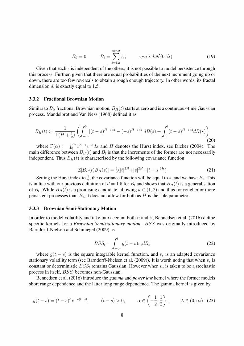
3.3.3 Brownian Semi-Stationary Motion

In order to model volatility and take into account both α and β, Bennedsen et al. (2016) definespecific kernels for a Brownian Semistationary motion. BSS was originally introduced byBarndorff-Nielsen and Schmiegel (2009) as

BSSt =

∫ t

−∞g(t− s)vsdBs (22)

where g(t − s) is the square integrable kernel function, and vs is an adapted covariancestationary volatility term (see Barndorff-Nielsen et al. (2009)). It is worth noting that when vs isconstant or deterministic BSSt remains Gaussian. However when vs is taken to be a stochasticprocess in itself, BSSt becomes non-Gaussian.

Bennedsen et al. (2016) introduce the gamma and power law kernel where the former modelsshort range dependence and the latter long range dependence. The gamma kernel is given by

g(t− s) = (t− s)αe−λ(t−s), (t− s) > 0, α ∈(−1

2,1

2

), λ ∈ (0,∞) (23)

8

where α is the roughness index and λ the memory parameter. The theoretical ACF of thegamma-kernel is defined as

ρgamma(h) =

(|h|2λ

)α+1/2

Kα+1/2(λ|h|)

(2λ)−2α−1π(24)

where Kv(x) is the modified Bessel function of the third kind. This gamma BSS process issaid to have short term memory as its ACF decays exponentially fast in the limit,

ρ(h)∼e−λhhα, h→∞ (25)

The power law kernel is given by

g(t−s) = (t−s)α(1 + (t−s))−γ−α, (t−s) > 0, α ∈(−1

2,1

2

), γ ∈

(1

2,∞)

(26)

where γ is the memory parameter. The ACF of the power law kernel is given by

ρpower(h) =

∫∞0g(x)g(x+ |h|)dx

B(2α + 1, 2γ − 1)(27)

where B(x, y) =∫ 1

0tx−1(1 − t)y−1dt. The autocorrelation functions are included here as

they are required in order to forecast volatility later on.It is now apparent why the BSS process under a gamma or power law kernel should provide

significantly better forecasts. The kernels allow both roughness and persistence to enter separatelyinto a covariance stationary stochastic process. Therefore, we should expect models driven by aBSS process to perform better than if they were driven by BH(t) or Bt.

3.4 SimulationThe accurate and efficient simulation of stochastic processes is vital, especially when pricingderivatives for which no closed form solution is available. In this case one has to resort to MonteCarlo simulation to generate a large number of possible price paths, compute the path’s exercisevalue and average these out in order to get the expected payoff of the derivative. Intuitively, themore price paths the better the approximation will be. Hence, efficiency is a sought after attributein simulation methods.

Regarding the three processes introduced in the previous section, one can differentiatebetween Bt which has independent increments and BH(t) as well as BSS which have correlatedincrements. When simulating dependent processes such as the latter two, we have to take intoaccount the correlation between increments. This can be done via either exact or approximateestimation methods.

An example of an exact simulation method is the Cholesky decomposition, which entailscomputing the process’s covariance matrix for the entire sample path using the theoreticalautocovariance function. This is computationally intensive since a sample path of length Nrequires a covariance matrix of dimension N ×N . A much more efficient method would be to

9

discretise the process in question and use Riemann sums to approximate each realization. Inthe case of the BH(t) and BSS process, efficiency can be further improved by realizing thatthese are convolutions. Hence, using the Fast Fourier Transform (FFT) one can convert thediscretized process into the frequency domain, where a convolution in the time domain becomesa multiplication, and once solved convert it back into the time domain using the inverse FFT.Bennedsen et al. (2015) further improved the accuracy of the Riemann approach by combining itwith exact simulation, which he calls the hybrid scheme. Bennedsen et al. (2016) notice that inthe particular case that the kernel g(x) behaves as a power-law function near zero, as x→ 0, theRiemann sum fails to approximate the kernel. Hence using exact simulation for the first coupleof steps before switching to the Riemann sum approximation significantly improves the accuracywhile remaining much more efficient than the Cholesky decomposition.

Figure 3 shows some simulations of BM, fBM with different values of α and BSS comparedto the realised kernel of the FTSE MIB, as an example of the historical pattern of asset volatility.It is easy to see that the volatility of the equity index is poorly modelled by standard Brownianmotion. By altering the Hurst parameter (reflected by the corresponding α value), fBM canproduce rougher simulations that are more realistic to the volatility of equity indices. The BSSsimulation is also able to replicate this roughness. In the Results section we will discuss in detailhow to calibrate these processes to a given time series, such as these equity indices.

4 Data SetWe downloaded daily realised variances for 21 equity indices from around the world from theperiod January 2000 to May 2017. The full sample includes: S&P 500, FTSE 100, Nikkei225, DAX, Russel 2000, All Ordinaries, DJIA, Nasdaq 100, CAC 40, Hang Seng, KOSPIComposite, AEX Index, Swiss Market, IBEX 35, S&P CNX Nifty, IPC Mexico, Bovespa,S&P/TSX Composite, Euro STOXX 50, FT Straits Times and FTSE MIB. Seventeen are largecap indices, one small cap (Russell 2000) and three indices are a mixture of large and small-caps.Eight indices are based on companies from Europe, four from the US, four from Asia, and the restare based on companies from Brazil, Canada, Australia and Mexico. In terms of methodology,80% are calculated based on a market capitalisation weighting, while the others are computedusing a metric based on either price or trading volume.

The realised volatilities are based on 5-minute prices and were downloaded from the Oxford-Man Institute’s Realized Library data, available at http://realized.oxford-man.ox.ac.uk/. Foreach of these 21 indices the Oxford Man Institute’s Realised library records daily returns, dailyrealised variances and daily realised kernels. We use the daily returns and the daily realisedkernel, introduced by Barndorff-Nielsen et al. (2008), as it has some robustness to the effects ofmarket micro-structure effects. See Heber et al. (2009) for more detail on how these measuresare computed. See Shephard and Sheppard (2010) and Barndorff-Nielsen et al. (2009) for morebackground on the realised measures.

If the market was closed or the data was regarded as being of too low quality for that index thedatabase shows a missing value (NA), except for days when all the markets are simultaneouslyclosed, in which case the day is not recorded in the database. As a result, for example, Saturdaysare never present in the library. The full time period left us with 4521 observations, excluding a

10

number of missing values which varied across index. All missing values were dropped beforeconducting our analysis. We also extracted index return data from the same source.

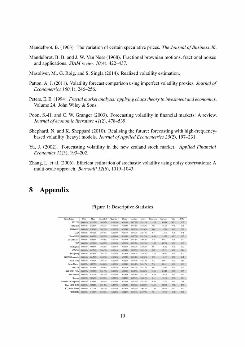
Figure 1 reports the basic summary statistics for the 21 stock indices in our sample. Therange of realised volatility varies quite considerably across indices over the full time period. Forexample, the S&P 500 had a minimum daily volatility of 0.0002% and a maximum of 0.9313%with a mean of 0.0111%, standard deviation of 0.0255%, a positive skewness of 15.05, anda kurtosis of 426.84. The FTSE 100 volatility in the sample period ranged from 0.0002% to0.3256%, with a mean of 0.0084%. We note that the skewness and the kurtosis of the seriesimply some deviation from a standard Gaussian distribution. Some deviations from normalityalso become apparent when we plot QQ plots of the series. Figure 2 shows the QQ Plot for the S& P 500 series as an illustration.

5 Results

5.1 Estimation of the BSS ModelTo fit the BSS model to the data described in Section 4 we must estimate the model parametersintroduced in section 3, namely the roughness parameters α and β and the memory parameter λ.In doing so we closely follow the procedures outlined in Bennedsen et al. (2016).

Recall that the roughness parameter α introduced in Equation (14) can be estimated by takingthe natural logarithm on both sides, leading to the OLS regression Equation (15):

log(1− ρ(h)) = c+ a log|h|+εh, h = ∆, 2∆, . . . ,m∆ (28)

where ρ(h) is the empirical autocorrelation function at lag h. For the step size we chose∆ = 1 day such that each lag corresponds to one day for a bandwidth of m = dn1/3e ≈ 17 days,where n corresponds to the number of observations for each vector (ticker) under considerationand d·e the ceiling.

We run the regression for each of the 21 tickers in our dataset and recover alpha using therelationship α = (a− 1)/2. Figure 4 a) shows the OLS regression results for the S&P 500 asan illustration. The full set of alpha estimates are in Figure 4 b). We find that there is somesubstantial variation in α across the 21 indices. The smoothest ticker is the Swiss Market Index,with an estimated alpha of −0.3268. The roughest series is the Australian All Ordinaries with anestimated alpha of −0.4228, close to the roughest possible value of −0.5 (corresponding to aHurst index of 0). The average alpha estimate across the full cross section is −0.3706, indicatingthat the volatility of equity indices is indeed rough.

We also investigated patterns across region of stock index, by type of index (i.e. large-cap,small-cap or all), and by methodology of index. Figure 5 illustrates the estimated parametervalues by geographic region. There were no strong patterns by type or methodology. We didnotice, perhaps unsurprisingly, that stock indices from similar regions, particularly all thoseindices covering US companies, reported similar estimate levels of roughness and persistence involatility over the 2000-2017 sample period analysed.

A natural question is whether the estimates of alpha change over time. In order to answer thisquestion we estimated alpha on a rolling basis for each security using a window of 60 consecutive

11

trading days. Figure 6 shows the trailing 60 trading days alpha estimates for the S&P 500. Wefind that alpha does substantially vary over time. The estimates broadly fall within the bound(−0.5,−0.1). Recall that a value of alpha close to −0.5 implies roughness and −0.1 smoother.In line with the findings in Bennedsen et al. (2016), we observe several peaks of smoothenessthat coincide with periods of market turmoil. For example there is a clear peak of alpha aroundthe Lehman collapse in 2008. We estimated the rolling variance for all the 21 equity indices andfind that the same pattern that volatility exhibits less roughness during market turmoil. This isagain in line with the findings of Bennedsen et al. (2016) and Gatheral et al. (2014). Of coursethe periods of market turmoil can be different across markets. For example we noted a higheralpha peak corresponding to the dotcom bubble of the early 2000s in the NASDAQ 100 whencompared to the other U.S. indices which have less focus on the technology sector.

Next we estimated the beta parameter over the entire sample to gauge the persistence of theunderlying series, see Figure 4 c). Recall that Equation (18) allows us to estimate beta usingsimple OLS. The findings reported in Figure 4 c) are estimated for M = m to M ′ = m+ 9 (notethat m in our sample corresponds to 17). We obtain the highest beta of approximately 0.5 forthe Nikkei. We obtain the lowest reading for the TSX Composite index, which compares to anaverage beta of 0.1996 for all 21 indices. These results differ from the findings in Bennedsenet al. (2016). The reason behind this difference can be found in the very large sensitivity ofBeta estimates with respect to the estimation window defined by M and M ′, and of coursethe underlying data. To illustrate the sensitivity of beta estimates we have calculated betas forall 21 indices fixing M to 17 and varying M’ from 26 to 278 representing an autocorrelationwindow ranging from 10 days to one year. Figure 7 shows our results. Indeed we find the betaestimates to vary substantially and we confirm that beta estimates are highly sensitive to thechoice of estimation range M to M ′. Theory suggests the choice of large M . We repeated theexercise for a window of M = 1 to M = m ≈ 17 and find results closer to the ones reported inBennedsen et al. (2016). Here, the KOSPI Composite index exhibits the highest persistence withan estimated beta of 0.0636. On the other extreme is the Bovespa index with a beta of 0.1942.The overall sample beta mean is 0.1079, indicating a relatively high persistence overall.

Lastly we estimate the memory parameter, λ for the gamma (and power) kernel BSS models.Lambda can be estimated by a methods-of-moments (MoM) procedure. Following Bennedsenet al. (2016) we use the previously fitted alpha estimates from above to plug them into thetheoretical autocorrelation function for the gamma kernel in Equation (24). The next step is tomatch the theoretical and the empirical ACF and minimize the squared differences over lambda.2

The results are shown in Figure 4 d). The results range from the lowest reading for the SwissMarket Index, 0.0041, to a maximum of 0.0230 for the Bovespa, with a mean of 0.0101. Notethat a small lambda would imply a model with long memory. We find that the estimates of λ arehighly sensitive to the choice of the lag of the ACF, ρ(h)), in equation (15), which impacts onthe functionality of the BSS model (discussed in more detail in the next section).

Having estimated all the relevant parameters, we are now able to construct the modelcalibrations for the fBM and gamma-kernel BSS specifications. For example Figure 8 showsour results for the estimated values of the S&P 500 using 500 i.i.d. drafts of a multivariateGaussian vector with mean zero and covariance matrix as described in Bennedsen et al. (2015).2This has been done using the autocorr and fmincon commands in matlab

12

The Truncated BSS (TBSS) model and the BSS trajectories shown in Figure 8 make use ofa modelling technique, referred to as hybrid scheme introduced in Bennedsen et al. (2015).The hybrid scheme discretises the stochastic integral in the time domain and approximates thefirst kappa steps by a power function near zero and a standard Riemann approximation after.The TBSS process is an extension to the BSS process with applications in rough Bergomimodels. The TBSS process allows us to directly compare the trajectories generated with theHybrid Scheme with those of the Riemann approximations. The red lines in the TBSS and BSSHybrid panels represent approximations setting kappa to 3. To compare the persistence fit ofthe BSS process we compared the empirical autocorrelation function with the autocorrelationfunction from the fitted processes. Figure 9 shows the results for the S&P 500. The BSS modelsatisfyingly replicates the autocorrelation pattern of the empirical ACF.

More important than simulating the processes with fitted parameters, we are now able toconduct forecasts using the BSS model.

5.2 Forecasting with BSSIn this section we use the BSS process to forecast realised variance and then evaluate the forecastaccuracy of the model and compare it against a series of benchmarks. We do this in a few steps.First, we conduct an in-sample forecast. We use the entire in-sample dataset to estimate theparameter for the models. Second, we use those parameters to forecast the realised varianceh steps ahead. Finally, we compare the Mean Square Error (MSE) and Quasi-likelihood (QL)against a set of benchmark models. Let us discuss these steps in turn before reporting the results.

Firstly, to forecast with the BSS process we assume Gaussianity of the processes andfollow the steps taken in Bennedsen et al. (2016). In particular we rely on the fact that for azero-mean Gaussian vector (xt+h, xt, xt−1, ..., xt−m)T the distribution of xt+h conditionally on(xt+h, xt, xt−1, ..., xt−m)T = a ∈ Rm+1 is

Xt+h|[xt, xt−1, ..., xt−m)T = a] ∼ N (µ,Ξ2) (29)

where µ = Γ12 · Γ−122 · a = Z · a, and Γ22 is the correlation matrix of the vector a and

Γ12 = [ρxt+h,xt , ρxt+h,xt−1 , ..., ρxt+h,xt−m ], where the correlations are obtained from the theoreticalcorrelation functions given in equation (24) and (27). The variance term is given by Ξ2 =Var(xt) ∗ (1− Γ12Γ−1

22 Γ21) where, Γ21 = ΓT12. 3

In the forecasting exercise we need a window of m previous data points on which we canthen compute an h step ahead forecast. The m is a rolling window and the parameters (e.g. α, λ)for the model are computed from the full data in ex-ante.

In order to retrieve the BSS process from our dataset we first take the square root to arrive atvolatility. Next we drop empty observations to remain consistent with the estimation of modelparameters, recall that we construct a series of consecutive trading days. For any index, thisleaves us with the vector for variances, σ. Recall the relation between volatility and BSS-processas stated in Equation (2). Thus, to recover the realised BSS-process, {X}t∈{1,...,T}, we first take

3To implement this matrix multiplication in practice we use the ’fliplr’ command in Matlab on the Γ)12 matrix toensure the correct time order of correlation lags.

13

the natural logarithm and then de-mean the vector as shown below:

lnσ =

lnσ1...

lnσT

, X =

[I − 1

Tii′]

lnσ

where i denotes the unit vector of size T , i′ its transpose and I the identity matrix. The resultfollows from 1/T

∑Tt=1 lnσt = 1/T

∑Tt=1 ln ξ + Xt = ln ξ + 1/T

∑Tt=1 Xt = lnξ and zero

mean property of the BSS process. 4

From this new vector X we feed the rolling window a. Note that the functional form ofvolatility given in Equation (2), requires us to forecast a log-normal distributed process. Toaccount for this we make use of the moment generating function and obtain our forecastsaccording to:

E[exp(Xt+∆|Ft)] = exp(E[Xt+∆|F ] +

1

2Var[Xt+∆|F ]

)(30)

This term is then approximated by inserting µ and Ξ2 from above. Pre-multiplying the h-stepahead forecast vector obtained in this fashion by ξ from the de-meaning step, we get the forecastvector for realised volatility σt+h.

Once we have the model estimated, the second step is to forecast ahead with it. We forecastone-step ahead (i.e. h=1) recursively, re-estimating the model each time based on the newupdated information set. We start forecasting after 200 periods of observations.

The final step of the forecasting methodology is to compute the loss functions. Here, we usetwo Patton class loss functions:5 the Mean Square Error (MSE), defined as

MSE : L(σ2t , σ

2t|t−1) = (σ2

t − σ2t|t−1)2; (31)

and the Quasi Likelihood (QL) loss function, defined as:

QL : L(σ2t , σ

2t|t−1) =

σ2t

σ2t|t−1

− log σ2t

σ2t|t−1

− 1. (32)

We identified some calibration issues stemming from the Method of Moments (MoM)estimation of λ that impact on our ability to forecast with the Gamma-BSS model. Afterthorough exploration of the Bennedsen et al. (2016) methodology we noticed forecast errorsexploding for some series and isolated λ estimation as the driving force. To further evaluatethe problem we calculated the MSEs for a range of λ from 0.0005 to 0.05 in steps of 0.0001,see Figure 11. The peak in the first plot shows the critical range around which forecast errorsexplode. Plot 2 shows the MSE on a logarithmic scale. We find the left hand side of the peakdoes not contain a global minimum. By zooming in on the right hand side, as shown in plot3, we find the global minimum (i.e. the point with lowest MSE). Note that this value for λ isfar from the minimum identified by MoM. Our findings suggest MoM might not be suited foroptimal forecasting results.4We ran Jarque–Bera normality tests on the realisedX process for the 21 series and reject the null of normality inall cases except one.

5Patton (2011) derives a class of loss functions that can be used to rank volatility models.

14

5.3 Forecasting PerformanceAfter estimating each model from the in-sample data, one-step ahead conditional volatilityforecasts are produced for the out-of-sample period. The λ estimation issue, described above,allows us to produce one-step ahead forecasts for six indices, namely: S&P 500; NASDAQ 100;Bovespa; AEX; Swiss Market; FTSE MIB. These six provide a decent geographical coverageof major equity markets. Figure 10 shows the results for the forecasting exercise. The BSSforecast performance appears to be very good for these indices, with one-step ahead forecastedvalues very close to the realised values. To evaluate this forecast performance in more depth weintroduce three benchmark models of volatility.

• Rolling Volatility: calculated as the standard deviation of the returns of the last 200consecutive trading days

σrolling,t+1 = std(Returns(t− 200 : t)) (33)

• Exponential Weighted Moving Average (EWMA): with a value of λ = 0.94. We take thesquare root of σ2

EWMA to obtain volatility.

σ2EWMA,t+1 = λ · σEWMA,t + (1− λ) · (Returns2

t ) (34)

• Log HAR model specification: where next period’s log volatility is based on a weightedaverage of the average log volatility over the last day, week and month. We take theexponent of σlogHAR to obtain volatility.

σLogHAR,t+1 = β0 + β1 · σDAY,t−1 + β2 · σWEEK,t−1 + β3 · σMONTH,t−1 (35)

The first two provide more traditional benchmarks. The third is a more recent state-of-the artvolatility model that should be harder to beat.

Table 1 reports the MSE and QL losses of the three benchmarks and the BSS model forthe one-step and ten-step ahead forecasts of the six indices. Looking first at the MSEs for theone-step ahead forecast, BSS outperforms all three benchmarks for the Swiss Market index. Itoutperforms the rolling volatility and EWMA, but not the Log-HAR, for the S& P 500, Nasdaq100 and the Bovespa. The BSS has a lower MSE than the rolling variances, but a higher MSEthan the Log-HAR and very similar MSE to the EWMA, for the FTSE MIB and AEX. Thispattern is repeated if we consider the QL loss function. In short the BSS is either the bestperformer or nearly as good as the Log-HAR specification. For the ten-step ahead forecast, theBSS outperforms all three benchmarks under both the MSE and the QL loss function for five ofthe six indices.

Next, we investigate if this BSS forecast out-performance versus some of benchmarks isstatistically significant. Diebold and Mariano (1995) introduce a test to assess if the forecastingability of two series is statistically different. The test enables us to see if model out-performanceagainst benchmarks is statistically significant. The null hypothesis is that two forecastingstrategies have the same predictive ability. Table 2 reports the DM-statistics and the correspondingp-values. For the one-step ahead forecast, the BSS statistically outperforms the rolling volatility

15

model for all six indices at a 5% significance level. BSS statistically outperforms the EWMA forthe Nasdaq, Swiss Market Index and Bovespa indices and the Log-HAR in the case of SwissMarket Index. However, the Log-HAR is statistically better than BSS for the other five indices.For the ten-step ahead forecast the BSS outperformance is closer to the Log-HAR benchmarkand under the MSE loss function it is significantly better for AEX, Swiss Market Index andFTSE MIB. Under the QL loss function the BSS significantly outperforms for all benchmarksfor all series.

6 ConclusionThis project confirms the findings of Gatheral et al. (2014) and Bennedsen et al. (2016) thatvolatility is indeed both rough and persistent across a wide range of equity indices. We haveexplored the advantage of using a Brownian Semi-Stationary (BSS) process to model volatilityenabling the user to calibrate both stylised facts in contrast to previous generations of fractalprocesses, like Fractional Brownian Motion. We have successfully implemented simulationmethods so that a BSS process can be incorporated within a continuous time asset pricingequation to price options and other exotic derivatives. We then calibrated the parameters for theBSS model using the realised kernel of 21 equity indices. Our parameter estimates confirm theexpected roughness and persistence in the series. The parameter for roughness, α, was quitestable across the cross-section of indices, but fluctuated over time. α averaged -0.37 and rangedfrom −0.33 to −0.42, implying much more roughness than the α = 0 implied by StandardBrownian Motion. Estimates of the long memory parameter, λ, were less stable, ranging from0.0041 to 0.0230. We identify an issue when using MoM estimation that suggests MoM maybe sub-optimal for BSS-Gamma forecasting. We forecast with six indices that cover a broadgeographical spread and have stable lambda estimates. For the one-step ahead forecast we findthat the BSS model outperformed two of our three benchmarks consistently under both MSEand QL loss functions. The BSS beat the Log-HAR benchmark in the case of the index with thelongest memory, while it was slightly worse for the other five indices. For the ten-step aheadforecast, under the MSE loss function, the BSS model outperformed all benchmarks consistentlyfor five out of six indices. Under the QL loss function the BSS outperforms all benchmarks, andthis outperformance is always statistically significant.

Areas for further research would include investigating the forecasting accuracy of the BSSPower Kernel using a wider range of asset class, such as commodities, real estate funds andforeign exchange rates. Further robustness checks could test the performance of BSS againstthe family of fractional volatility models. It would also be interesting to further explore therelationship of ξ and its link with the variance swap curve.

7 ReferencesAndersen, T. G. and T. Bollerslev (1998). Answering the skeptics: Yes, standard volatility

models do provide accurate forecasts. International economic review, 885–905.

16

Andersen, T. G., T. Bollerslev, F. X. Diebold, and P. Labys (2001). The distribution of realizedexchange rate volatility. Journal of the American statistical association 96(453), 42–55.

Andersen, T. G., T. Bollerslev, F. X. Diebold, and P. Labys (2003). Modeling and forecastingrealized volatility. Econometrica 71(2), 579–625.

Baillie, R. T., T. Bollerslev, and H. O. Mikkelsen (1996). Fractionally integrated generalizedautoregressive conditional heteroskedasticity. Journal of econometrics 74(1), 3–30.

Barndorff-Nielsen, O. E. (2002). Econometric analysis of realized volatility and its use inestimating stochastic volatility models. Journal of the Royal Statistical Society: Series B(Statistical Methodology) 64(2), 253–280.

Barndorff-Nielsen, O. E., P. R. Hansen, A. Lunde, and N. Shephard (2008). Designing re-alized kernels to measure the ex post variation of equity prices in the presence of noise.Econometrica 76(6), 1481–1536.

Barndorff-Nielsen, O. E., P. R. Hansen, A. Lunde, and N. Shephard (2009). Realized kernels inpractice: Trades and quotes. The Econometrics Journal 12(3), C1–C32.

Barndorff-Nielsen, O. E. and J. Schmiegel (2009). Brownian semistationary processes andvolatility/intermittency. Advanced financial modelling 8, 1–25.

Bayer, C., P. Friz, and J. Gatheral (2016). Pricing under rough volatility. Quantitative Fi-nance 16(6), 887–904.

Bennedsen, M., A. Lunde, and M. S. Pakkanen (2015). Hybrid scheme for brownian semista-tionary processes. arXiv preprint arXiv:1507.03004.

Bennedsen, M., A. Lunde, and M. S. Pakkanen (2016). Decoupling the short-and long-termbehavior of stochastic volatility. SSRN.

Beran, J. (1994). Statistics for long-memory processes, Volume 61. CRC press.

Black, F. and M. Scholes (1973). The pricing of options and corporate liabilities. Journal ofpolitical economy 81(3), 637–654.

Bollerslev, T. (1986). Generalized autoregressive conditional heteroskedasticity. Journal ofeconometrics 31(3), 307–327.

Comte, F. and E. Renault (1996). Long memory continuous time models. Journal of Economet-rics 73(1), 101–149.

Comte, F. and E. Renault (1998). Long memory in continuous-time stochastic volatility models.Mathematical Finance 8(4), 291–323.

Di Matteo, T., T. Aste, and M. Dacorogna (2003). Scaling behaviors in differently developedmarkets. Physica A: Statistical Mechanics and its Applications 324(1), 183–188.

17

Dicker, T. (2004). Simulation of fractional Brownian motion. Ph. D. thesis, University of Twente.

Diebold, F. X. and R. S. Mariano (1995, July). Comparing Predictive Accuracy. Journal ofBusiness & Economic Statistics 13(3), 253–263.

Ding, Z., C. W. Granger, and R. F. Engle (1993). A long memory property of stock marketreturns and a new model. Journal of empirical finance 1(1), 83–106.

Duffie, D. and K. J. Singleton (1993). Simulated moments estimation of markov models of assetprices. Econometrica: Journal of the Econometric Society, 929–952.

El Euch, O., M. Fukasawa, and M. Rosenbaum (2016). The microstructural foundations ofleverage effect and rough volatility. arxiv preprint. arXiv preprint arXiv:1609.05177.

Engle, R. F. (1982). Autoregressive conditional heteroscedasticity with estimates of the varianceof united kingdom inflation. Econometrica: Journal of the Econometric Society, 987–1007.

Fama, E. F. (1965). The behavior of stock-market prices. The journal of Business 38(1), 34–105.

Gatheral, J., T. Jaisson, and M. Rosenbaum (2014). Volatility is rough. working paper.

Granger, C. W. (2000). Advances in Statistics, Combinatorics and Related Areas, Chapter LongMemory Processes-an Economist’s Viewpoint, pp. 100. World Scientific Pub Co Inc.

Harvey, A. C. (1998). Long Memory in Stochastic Volatility, Chapter 16 in ’Forecasting Volatilityin the Financial Markets’, pp. 307–320. Butterworth Heinemann.

Heber, G., A. Lunde, N. Shephard, and K. Sheppard (2009). Oxford-man institute’s realizedlibrary, version 0.1.

Heynen, R. C. (1995). Essays on derivatives pricing theory. Ph. D. thesis.

Heynen, R. C. and H. M. Kat (1994). Volatility prediction: a comparison of the stochasticvolatility, garch (1, 1) and egarch (1, 1) models. The Journal of Derivatives 2(2), 50–65.

Hull, J. and A. White (1987). The pricing of options on assets with stochastic volatilities. Thejournal of finance 42(2), 281–300.

Hull, J. and A. White (1988). An analysis of the bias in option pricing caused by a stochasticvolatility. Advances in futures and options research 3(1), 29–61.

Hurst, H. E., R. P. Black, and Y. Simaika (1965). Long-term storage: an experimental study.Constable.

Hwang, S. and S. E. Satchell (1998). Forecasting volatility in the financial markets. pp. 193–225.

Jacod, J., Y. Li, P. A. Mykland, M. Podolskij, and M. Vetter (2009). Microstructure noise inthe continuous case: the pre-averaging approach. Stochastic processes and their applica-tions 119(7), 2249–2276.

18

Mandelbrot, B. (1963). The variation of certain speculative prices. The Journal of Business 36.

Mandelbrot, B. B. and J. W. Van Ness (1968). Fractional brownian motions, fractional noisesand applications. SIAM review 10(4), 422–437.

Masoliver, M., G. Roig, and S. Singla (2014). Realized volatility estimation.

Patton, A. J. (2011). Volatility forecast comparison using imperfect volatility proxies. Journal ofEconometrics 160(1), 246–256.

Peters, E. E. (1994). Fractal market analysis: applying chaos theory to investment and economics,Volume 24. John Wiley & Sons.

Poon, S.-H. and C. W. Granger (2003). Forecasting volatility in financial markets: A review.Journal of economic literature 41(2), 478–539.

Shephard, N. and K. Sheppard (2010). Realising the future: forecasting with high-frequency-based volatility (heavy) models. Journal of Applied Econometrics 25(2), 197–231.

Yu, J. (2002). Forecasting volatility in the new zealand stock market. Applied FinancialEconomics 12(3), 193–202.

Zhang, L. et al. (2006). Efficient estimation of stochastic volatility using noisy observations: Amulti-scale approach. Bernoulli 12(6), 1019–1043.

8 Appendix

Figure 1: Descriptive Statistics

Stock Index Min Max Quartile 1 Quartile 3 Mean Median Stdev Skewness Kurtosis Obs NAs

S&P 500 0.0002% 0.9313% 0.0026% 0.0109% 0.0111% 0.0052% 0.0255% 15.05 426.84 4521 198

FTSE 100 0.0004% 0.3256% 0.0022% 0.0088% 0.0084% 0.0041% 0.0152% 7.92 101.26 4521 175

Nikkei 225 0.0004% 0.3836% 0.0039% 0.0125% 0.0114% 0.0070% 0.0190% 8.66 110.24 4521 328

DAX 0.0003% 0.6432% 0.0049% 0.0180% 0.0177% 0.0093% 0.0314% 8.44 114.73 4521 141

Russel 2000 0.0000% 0.6425% 0.0032% 0.0104% 0.0108% 0.0055% 0.0217% 10.93 213.82 4521 195

All Ordinaries 0.0001% 0.1556% 0.0015% 0.0051% 0.0049% 0.0026% 0.0083% 7.46 84.95 4521 197

DJIA 0.0002% 0.9126% 0.0027% 0.0103% 0.0107% 0.0051% 0.0255% 15.15 407.24 4521 195

Nasdaq 100 0.0000% 0.6669% 0.0029% 0.0137% 0.0135% 0.0057% 0.0262% 8.97 146.32 4521 192

CAC 40 0.0004% 0.4551% 0.0043% 0.0161% 0.0145% 0.0083% 0.0231% 7.67 93.78 4521 114

Hang Seng 0.0004% 0.4461% 0.0032% 0.0092% 0.0088% 0.0052% 0.0162% 14.04 300.46 4521 527

KOSPI Composite 0.0004% 0.6479% 0.0029% 0.0148% 0.0133% 0.0067% 0.0238% 9.78 181.06 4521 261

AEX Index 0.0003% 0.3962% 0.0033% 0.0132% 0.0126% 0.0063% 0.0217% 6.52 66.01 4521 115

Swiss Market 0.0007% 0.2797% 0.0026% 0.0082% 0.0084% 0.0042% 0.0145% 7.16 81.32 4521 189

IBEX 35 0.0004% 0.4766% 0.0048% 0.0177% 0.0150% 0.0100% 0.0213% 8.04 110.57 4521 149

S&P CNX Nifty 0.0003% 1.0108% 0.0041% 0.0143% 0.0148% 0.0073% 0.0328% 13.86 313.12 4521 775

IPC Mexico 0.0003% 0.3010% 0.0024% 0.0069% 0.0066% 0.0038% 0.0112% 10.53 193.04 4521 194

Bovespa 0.0008% 0.8364% 0.0098% 0.0249% 0.0238% 0.0154% 0.0384% 9.44 131.82 4521 289

S&P/TSX Composite 0.0000% 0.3545% 0.0014% 0.0050% 0.0056% 0.0024% 0.0144% 10.99 175.26 4521 781

Euro STOXX 50 0.0000% 1.0922% 0.0047% 0.0174% 0.0165% 0.0089% 0.0320% 13.65 342.42 4521 138

FT Straits Times 0.0006% 0.2773% 0.0021% 0.0064% 0.0057% 0.0035% 0.0087% 11.98 280.22 4521 642

FTSE MIB 0.0003% 0.4304% 0.0037% 0.0148% 0.0129% 0.0074% 0.0199% 7.84 107.97 4521 157

19

Figure 2: QQ Plot for S&P 500

-1 -0.5 0 0.5 1 1.5

Data

0.001

0.003

0.010.02

0.05

0.10

0.25

0.50

0.75

0.90

0.95

0.980.99

0.997

0.999

Pro

babi

lity

S&P 500 (Live)

Figure 3: Simulated Processes

0 50 100 150 200 250 300 350 400 450 5000

5

10FTSE MIB realised kernel

0 50 100 150 200 250 300 350 400 450 500-2

0

2Standard Brownian Motion alpha = 0

0 50 100 150 200 250 300 350 400 450 500-5

0

5Fractional Brownian Motion alpha = -0.15

0 50 100 150 200 250 300 350 400 450 500-5

0

5Fractional Brownian Motion alpha = -0.49

0 50 100 150 200 250 300 350 400 450 500-4

-2

0

2BSS

20

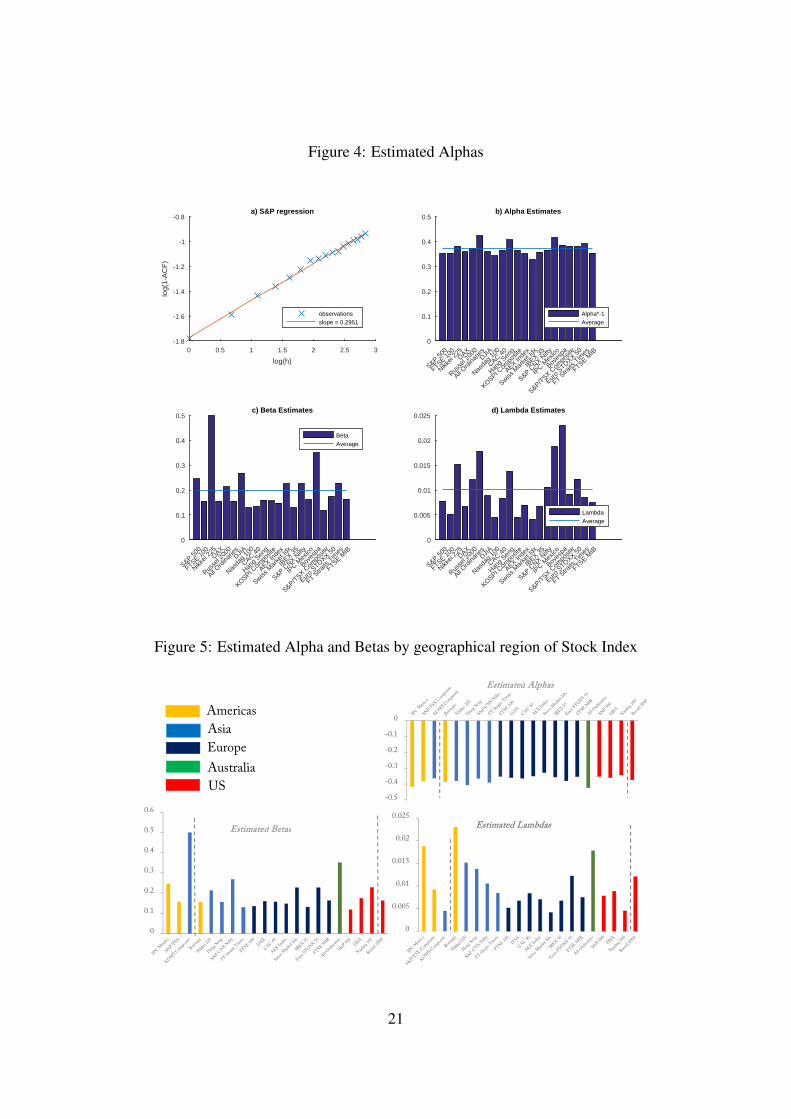
Figure 4: Estimated Alphas

0 0.5 1 1.5 2 2.5 3

log(h)

-1.8

-1.6

-1.4

-1.2

-1

-0.8

log(

1-A

CF

)

a) S&P regression

observationsslope = 0.2951

S&P 500

FTSE 100

Nikkei

225DAX

Russe

l 200

0

All Ord

inarie

sDJIA

Nasda

q 10

0

CAC 40

Hang

Seng

KOSPI Com

posit

e

AEX Inde

x

Swiss M

arke

t Idx

IBEX 3

5

S&P CNX N

ifty

IPC M

exico

Boves

pa

S&P/TSX C

ompo

site

Euro

STOXX 50

FT Stra

its T

imes

FTSE MIB

0

0.1

0.2

0.3

0.4

0.5b) Alpha Estimates

Alpha*-1Average

S&P 500

FTSE 100

Nikkei

225DAX

Russe

l 200

0

All Ord

inarie

sDJIA

Nasda

q 10

0

CAC 40

Hang

Seng

KOSPI Com

posit

e

AEX Inde

x

Swiss M

arke

t Idx

IBEX 3

5

S&P CNX N

ifty

IPC M

exico

Boves

pa

S&P/TSX C

ompo

site

Euro

STOXX 50

FT Stra

its T

imes

FTSE MIB

0

0.005

0.01

0.015

0.02

0.025d) Lambda Estimates

LambdaAverage

S&P 500

FTSE 100

Nikkei

225DAX

Russe

l 200

0

All Ord

inarie

sDJIA

Nasda

q 10

0

CAC 40

Hang

Seng

KOSPI Com

posit

e

AEX Inde

x

Swiss M

arke

t Idx

IBEX 3

5

S&P CNX N

ifty

IPC M

exico

Boves

pa

S&P/TSX C

ompo

site

Euro

STOXX 50

FT Stra

its T

imes

FTSE MIB

0

0.1

0.2

0.3

0.4

0.5c) Beta Estimates

BetaAverage

Figure 5: Estimated Alpha and Betas by geographical region of Stock Index

0

0.005

0.01

0.015

0.02

0.025Estimated Lambdas

0

0.1

0.2

0.3

0.4

0.5

0.6

Estimated Betas

-0.5

-0.4

-0.3

-0.2

-0.1

0

Estimated Alphas

AmericasAsiaEuropeAustraliaUS

21

Figure 6: Rolling Alpha S&P 500

30.03.2000

06.04.2001

24.04.2002

30.04.2003

04.05.2004

05.05.2005

05.05.2006

08.05.2007

07.05.2008

18.05.2009

18.05.2010

17.05.2011

16.05.2012

20.05.2013

20.05.2014

20.05.2015

19.05.2016

-0.55

-0.5

-0.45

-0.4

-0.35

-0.3

-0.25

-0.2

-0.15

-0.1Alpha (rolling estimate m=60)Simple Moving Average for n=60

Figure 7: Sensitivity Analysis Of the Beta Estimation

300

250

200

M' for M =m

1500

0.2

S&P 500

FTSE 100

Nikkei

225 100

DAX

0.4

Russe

l 200

0

All Ord

inarie

sDJIA

Nasda

q 10

0

CAC 40

0.6

Hang

Seng

Bet

a es

timat

e

KOSPI Com

posit

e

AEX Inde

x 50

Swiss M

arke

t Idx

IBEX 3

5

0.8

S&P CNX N

ifty

IPC M

exico

Boves

pa

S&P/TSX C

ompo

site

Euro

STOXX 50

1

FT Stra

its T

imes

FTSE MIB 0

1.2

0.1

0.2

0.3

0.4

0.5

0.6

0.7

0.8

0.9

1

22

Figure 8: Estimated Processes: S&P 500

0 50 100 150 200 250 300 350 400 450 500-5

0

5Standard Brownian Motion

0 50 100 150 200 250 300 350 400 450 500-5

0

5Fractional Brownian Motion

0 50 100 150 200 250 300 350 400 450 500-5

0

5BSS: Power Kernel (Riemann)

0 50 100 150 200 250 300 350 400 450 500-5

0

5BSS: Gamma Kernel (Riemann)

0 50 100 150 200 250 300 350 400 450 500-5

0

5TBSS: Gamma Kernel (Hybrid)

0 50 100 150 200 250 300 350 400 450 500-5

0

5BSS: Gamma Kernel (Hybrid)

The red lines for the TBSS and BSS processes show the estimation results for κ = 2. Thestandard deviation for the processes has been standardized to one. The deviation between TBSSand BSS paths results from required re-sampling the random vector.

Figure 9: Empirical vs. Simulated ACF

0 5 10 15 20

Lags

0

0.5

1

Em

piric

al A

CF

BSS kappa=3Empirical ACF

23

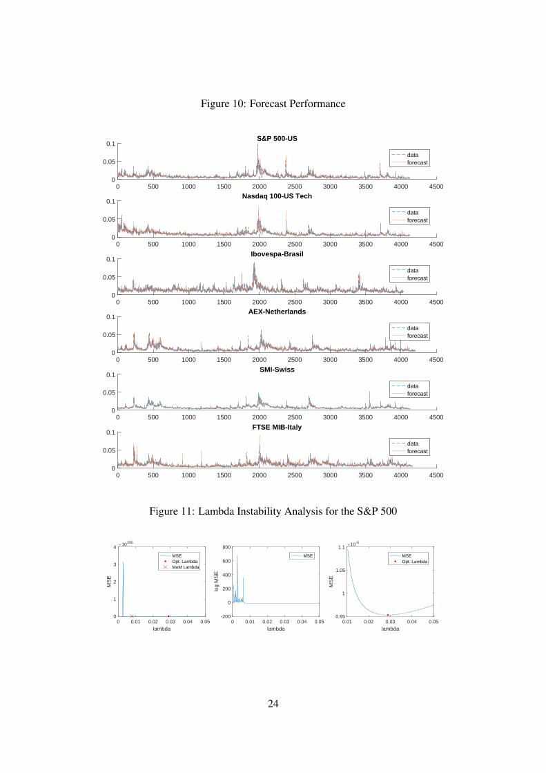
Figure 10: Forecast Performance

0 500 1000 1500 2000 2500 3000 3500 4000 45000

0.05

0.1S&P 500-US

dataforecast

0 500 1000 1500 2000 2500 3000 3500 4000 45000

0.05

0.1Nasdaq 100-US Tech

dataforecast

0 500 1000 1500 2000 2500 3000 3500 4000 45000

0.05

0.1Ibovespa-Brasil

dataforecast

0 500 1000 1500 2000 2500 3000 3500 4000 45000

0.05

0.1AEX-Netherlands

dataforecast

0 500 1000 1500 2000 2500 3000 3500 4000 45000

0.05

0.1SMI-Swiss

dataforecast

0 500 1000 1500 2000 2500 3000 3500 4000 45000

0.05

0.1FTSE MIB-Italy

dataforecast

Figure 11: Lambda Instability Analysis for the S&P 500

0 0.01 0.02 0.03 0.04 0.05

lambda

0

1

2

3

4

MS

E

#10295

MSEOpt. LambdaMoM Lambda

0 0.01 0.02 0.03 0.04 0.05

lambda

-200

0

200

400

600

800

log

MS

E

MSE

0.01 0.02 0.03 0.04 0.05

lambda

0.95

1

1.05

1.1

MS

E

#10-5

MSEOpt. Lambda

24

Table 1: Forecast Performance MSE and QL

Step Ahead = 1 Step Ahead = 10Index Metric Roll Var EWMA Log-HAR BSS Roll Var EWMA Log-HAR BSS

S&P 500 MSE 105 3.3097 1.6965 1.1210 1.5027 3.6087 2.5157 1.9031 1.8360QL 0.1130 0.0647 0.0470 0.0620 2.1791 0.0910 0.0831 0.0760

Nadaq MSE 105 3.2007 1.8984 0.9613 1.5115 3.4306 2.5622 1.5480 1.4946QL 0.1048 0.0621 0.0382 0.0532 2.1275 0.0811 0.0666 0.0621

AEX MSE 105 2.8307 1.4024 1.1152 1.4125 3.0980 2.3604 1.9472 1.8069QL 0.0929 0.0496 0.0413 0.0563 2.3901 0.0804 0.0724 0.0660

SMI MSE 105 1.7776 0.9667 0.6381 0.5116 1.9616 1.6739 1.2159 1.0790QL 0.0781 0.0407 0.0272 0.0221 2.4126 0.0697 0.0533 0.0481

Bovespa MSE 105 5.2725 3.1314 2.1369 2.5650 5.6765 4.4672 3.1737 3.2284QL 0.0821 0.0522 0.0415 0.0496 2.3689 0.0723 0.0612 0.0571

FTSE MSE 105 2.9630 1.6479 1.1311 1.8223 3.1910 2.5347 1.9233 1.7963MIB QL 0.0961 0.0552 0.0410 0.0659 2.2655 0.0803 0.0700 0.0658

Table 2: Diebold and Mariano (1995) test results Benchmarks vs. BSS forecast errors

Step Ahead = 1 Step Ahead = 10MSE QL MSE QL

Index Roll Var EWMA Log-HAR Roll Var EWMA Log-HAR Roll Var EWMA Log-HAR Roll Var EWMA Log-HARSP 500 10.6881 1.4007 -2.9181 17.9422 1.3288 -7.9014 19.8982 6.9068 1.0980 22.2359 9.2236 4.5126

(0.0000) (0.0807) (0.0018) (0.0000) (0.0920) (0.0000) (0.0000) (0.0000) (0.1361) (0.0000) (0.0000) (0.0000)Nasdaq 11.8380 2.8516 -4.4901 21.9667 5.0178 -9.3689 23.1087 10.2427 1.1575 26.0394 12.3021 3.4256

(0.0000) (0.0022) (0.0000) (0.0000) (0.0000) (0.0000) (0.0000) (0.0000) (0.1235) (0.0000) (0.0000) (0.0003)AEX 12.5481 -0.1349 -3.7990 13.3000 -3.5122 -8.2258 21.6140 9.0583 3.0580 21.0672 10.0088 5.1308

(0.0000) (0.4463) (0.0001) (0.0000) (0.0002) (0.0000) (0.0000) (0.0000) (0.0011) (0.0000) (0.0000) (0.0000)SMI 19.9699 14.5622 5.4946 28.9355 20.6586 6.6659 24.2836 13.5029 4.9721 25.4787 17.9922 7.0082

(0.0000) (0.0000) (0.0000) (0.0000) (0.0000) (0.0000) (0.0000) (0.0000) (0.0000) (0.0000) (0.0000) (0.0000)Bovespa 14.0738 4.5146 -3.6657 16.0881 1.7294 -5.5111 19.1422 7.3387 -0.4571 20.4261 11.1119 3.3737

(0.0000) (0.0000) (0.0001) (0.0000) (0.0419) (0.0000) (0.0000) (0.0000) (0.3238) (0.0000) (0.0000) (0.0004)FTSE 7.9916 -1.4069 -5.3118 10.2859 -4.6379 -10.9580 23.8457 12.3160 3.1201 20.3776 10.0739 3.6994MIB (0.0000) (0.0797) (0.0000) (0.0000) (0.0000) (0.0000) ’(0.0000) (0.0000) (0.0009) (0.0000) (0.0000) (0.0001)

Test statistics, p-values in parenthesis. Null hypothesis is no difference between forecast models.

25