Estimating Term Premia at the Zero

Bound: An Analysis of Japanese, US, and

UK Yields

Hibiki Ichiue* hibiki.ichiue@boj.or.jp Yoichi Ueno ** youichi.ueno@boj.or.jp

No.13-E-8 May 2013

Bank of Japan 2-1-1 Nihonbashi-Hongokucho, Chuo-ku, Tokyo 103-0021, Japan

** Monetary Affairs Department ** Monetary Affairs Department

Papers in the Bank of Japan Working Paper Series are circulated in order to stimulate discussion and comments. Views expressed are those of authors and do not necessarily reflect those of the Bank. If you have any comment or question on the working paper series, please contact each author.

When making a copy or reproduction of the content for commercial purposes, please contact the Public Relations Department (post.prd8@boj.or.jp) at the Bank in advance to request permission. When making a copy or reproduction, the source, Bank of Japan Working Paper Series, should explicitly be credited.

Bank of Japan Working Paper Series

1

Estimating Term Premia at the Zero Bound:

An Analysis of Japanese, US, and UK Yields*

Hibiki Ichiue†and Yoichi Ueno§

May 2013

Abstract

This paper estimates an affine term structure model (ATSM) and a shadow rate model

(SRM) using Japanese, US, and UK data until March 2013. These models produce very

different results, which are attributable to the ATSM’s neglect of the zero lower bound

(ZLB). The 10-year term premium estimated by the ATSM occasionally deviates from

that estimated by the SRM by around 2 percentage points, and the deviation has recently

widened in the US and the UK. The ATSM consistently overestimates the long-run level

of the short rate, which appears to contribute to the tendency to underestimate the term

premium.

JEL classification: E43; E52; G12

Keywords: Affine term structure model; Shadow rate model; Zero lower bound; Term

premium; Monetary policy

* We are grateful for helpful discussions with and comments from the staff of the Bank of Japan, in particular, Kentaro Kikuchi. The views expressed here are ours alone and do not necessarily reflect those of the Bank of Japan. † Bank of Japan (hibiki.ichiue@boj.or.jp) § Bank of Japan (youichi.ueno@boj.or.jp)

2

“An undesirable feature of the Gaussian model is that it implies that the short rate and

yields on bonds of any maturity are negative with positive probability at any future

date….Gaussian short-rate models are nevertheless useful, and frequently used, because

they are relatively tractable and in light of the low likelihood that they would assign to

negative interest rates within a reasonably short time…” (Duffie, 2001, p.140)

1. Introduction

Affine term structure models (ATSMs), introduced by Duffie and Kan (1996), are a very

popular tool for the analysis of the yield curve, not only in the literature of finance but

also in that of monetary economics. In particular, studies in the monetary economics

literature have become more dependent on ATSMs after many central banks such as the

Federal Reserve and the Bank of England faced the zero lower bound (ZLB) and started

to encourage a decline in long-term yields through asset purchases.

The literature suggests mainly two transmission channels through which asset

purchases lower long-term yields: the portfolio balance channel and the signaling

channel. Through the portfolio balancing channel, announcements of central bank bond

purchases lead market participants to expect a reduction in the supply of long-term bonds,

which pushes down the term premia. Through the signaling channel, announcements of

bond purchases provide information to market participants about future short-term

interest rates. For example, such announcements could signal that the central bank holds

a pessimistic view, so that market participants revise down their expectations of

short-term interest rates, which – as suggested by the expectations hypothesis – in turn

leads to a fall in long-term yields. To identify the transmission channels, term structure

models are essential: the literature utilizes ATSMs to decompose long-term yields into

expectations components, i.e., the averages of current and expected short-term interest

rates, and term premia.1

1 There is a long list of studies that have used a variety of ATSMs to examine the effects and the transmission channels of asset purchases of the Federal Reserve and the Bank of England. Gagnon et al. (2011) are the pioneers to investigate the Federal Reserve’s Large-Scale Asset Purchases (LSAPs). They show event study evidence that after eight key LSAP announcements in 2008 and 2009, the

3

Unfortunately, commonly-used Gaussian ATSMs, where the short rate follows a

Gaussian process, have the critical drawback that they allow negative interest rates or do

not take account of the ZLB.2 Such models may be a good first approximation when

interest rates are far from the ZLB. However, this precondition is no longer satisfied in

major developed economies. This means that, ironically, studies in monetary economics

started to rely more on ATSMs exactly when ATSMs became less reliable. Why do

studies in monetary economics rely to such an extent on ATSMs, which do not account

for the ZLB, when economies face the ZLB? Part of the reason is that the properties of,

and estimation methods for, ATSMs have been intensively examined in the literature,

while those of alternative models have been examined only to a limited extent. The

absence of prevailing alternative models makes it difficult to investigate how much

empirical results obtained from ATSMs suffer from the neglect of the ZLB. This may be

one factor responsible for the insufficient awareness of researchers regarding the

problems involved in using ATSMs.

Among term structure models taking account of the ZLB, shadow rate models

(SRMs) are a promising candidate. In typical SRMs, there is a shadow rate that can take 10-year yield fell by a total of 91 basis points, while the 10-year term premium, which is computed by updating the estimation of the ATSM studied by Kim and Wright (2005) and reported on the homepage of the Federal Reserve Board, fell by 71 basis points. Based on such evidence, Gagnon et al. (2011) argue that the LSAPs lowered long-term yields primarily through the portfolio balance channel. On the other hand, D’Amico et al. (2012) identify the transmission channels of the LSAPs utilizing regressions of the risk premia estimated based on the ATSM examined by D’Amico et al. (2010). Bernanke (2013) also uses the risk premia estimated employing the ATSM of D’Amico et al. (2010) to discuss the determinants of long-term interest rates, including the policies of the Federal Reserve. Other studies employing ATSMs to examine the effects of LSAPs include Bauer and Rudebusch (2011), Hamilton and Wu (2012), Li and Wei (2013), and Ihrig et al. (2012). Meanwhile, Joyce et al. (2011) identify the transmission channels of the Bank of England’s Asset Purchasing Program employing the term premia estimated using the ATSM studied by Joyce et al. (2010). Christensen and Rudebusch (2012) use ATSMs to investigate the difference in the transmission channels of the Federal Reserve’s LSAPs and the Bank of England’s Asset Purchasing Program. Bauer and Neely (2012) estimate ATSMs for six countries including the US and the UK to examine the channels through which the Federal Reserves’ LSAP announcements have effects on yields of those countries. 2 Some ATSMs, such as the one developed by Cox et al. (1985), have square root (i.e., non-Gaussian) processes. Although these models take the ZLB into account, they are much less popular than Gaussian ATSMs; in fact, all the studies mentioned in footnote 1 utilize Gaussian ATSMs. Part of the reason appears to be that ATSMs with square root processes are criticized for the difficulty in replicating the behavior of the short rate (Black 1995) and the distribution of bond yields (Kim and Singleton 2012). Against this background, when we refer to ATSMs in this paper we mean Gaussian ATSMs.

4

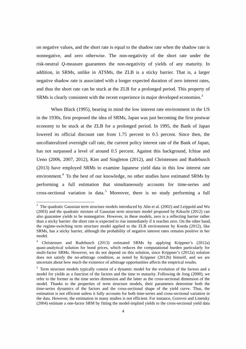
on negative values, and the short rate is equal to the shadow rate when the shadow rate is

nonnegative, and zero otherwise. The non-negativity of the short rate under the

risk-neutral Q-measure guarantees the non-negativity of yields of any maturity. In

addition, in SRMs, unlike in ATSMs, the ZLB is a sticky barrier. That is, a larger

negative shadow rate is associated with a longer expected duration of zero interest rates,

and thus the short rate can be stuck at the ZLB for a prolonged period. This property of

SRMs is clearly consistent with the recent experience in major developed economies.3

When Black (1995), bearing in mind the low interest rate environment in the US

in the 1930s, first proposed the idea of SRMs, Japan was just becoming the first postwar

economy to be stuck at the ZLB for a prolonged period. In 1995, the Bank of Japan

lowered its official discount rate from 1.75 percent to 0.5 percent. Since then, the

uncollateralized overnight call rate, the current policy interest rate of the Bank of Japan,

has not surpassed a level of around 0.5 percent. Against this background, Ichiue and

Ueno (2006, 2007, 2012), Kim and Singleton (2012), and Christensen and Rudebusch

(2013) have employed SRMs to examine Japanese yield data in this low interest rate

environment.4 To the best of our knowledge, no other studies have estimated SRMs by

performing a full estimation that simultaneously accounts for time-series and

cross-sectional variation in data. 5 Moreover, there is no study performing a full

3 The quadratic Gaussian term structure models introduced by Ahn et al. (2002) and Leippold and Wu (2003) and the quadratic mixture of Gaussian term structure model proposed by Kikuchi (2012) can also guarantee yields to be nonnegative. However, in these models, zero is a reflecting barrier rather than a sticky barrier: the short rate is expected to rise immediately if it reaches zero. On the other hand, the regime-switching term structure model applied to the ZLB environment by Koeda (2012), like SRMs, has a sticky barrier, although the probability of negative interest rates remains positive in her model. 4 Christensen and Rudebusch (2013) estimated SRMs by applying Krippner’s (2012a) quasi-analytical solution for bond prices, which reduces the computational burden particularly for multi-factor SRMs. However, we do not depend on this solution, since Krippner’s (2012a) solution does not satisfy the no-arbitrage condition, as noted by Krippner (2012b) himself, and we are uncertain about how much the existence of arbitrage opportunities affects the empirical results. 5 Term structure models typically consist of a dynamic model for the evolution of the factors and a model for yields as a function of the factors and the time to maturity. Following de Jong (2000), we refer to the former as the time series dimension and the latter as the cross-sectional dimension of the model. Thanks to the properties of term structure models, their parameters determine both the time-series dynamics of the factors and the cross-sectional shape of the yield curve. Thus, the estimation is not efficient unless it fully accounts for both time-series and cross-sectional variation in the data. However, the estimation in many studies is not efficient. For instance, Gorovoi and Linetsky (2004) estimate a one-factor SRM by fitting the model-implied yields to the cross-sectional yield data

5

estimation using yield data other than data for Japan’s low interest rate environment from

1995 onward.6

This paper contributes to the literature by performing a full estimation of an SRM

using data for Japan, the US, and the UK. The data cover the period from January 1990

to March 2013, which contains periods of both low and high interest rates. For Japan, as

mentioned above, the literature uses only data for the low interest rate environment. On

the other hand, our choice of observation period is suitable to make comparisons with the

empirical results for the US and the UK, where long data with low interest rates are not

available. Since even in periods of low interest rates, central banks typically do not set

the policy rate at exactly zero but at a small positive value, we allow the lower bound of

the short rate to deviate from exactly zero. We focus on two-factor models, following

Ichiue and Ueno (2007) and Kim and Singleton (2012). Three or more-factor models are

beyond the scope of this paper primarily because of the computational burden. Another

reason for focusing on two-factor models is that when interest rates are stuck at the ZLB

and do not move much, a large part of the information required to identify the factors is

missing, and thus the number of factors may have to be smaller than that when interest

rates are far from zero.7 We compare the estimation results of the SRM with those of an

ATSM. In particular, we are interested in how the ATSM’s neglect of the ZLB leads to a

biased decomposition of long-term interest rates into expectations components and term

premia. To examine the effects of the ZLB, the ATSM is also estimated using the data for

the pre-ZLB sub-period up to 2007 for the US and the UK. of Japan only at a selected date, February 3, 2002. Meanwhile, although Ueno et al. (2006) use daily data spanning a period of five years, they estimate the same model for each day and completely ignore the time-series developments of the yield data. Since their estimation accounts only for the cross-sectional variation in the data, the results obtained from such estimation are unreliable, as discussed by Ichiue and Ueno (2006, 2012). Krippner (2012b) uses nonlinear least squares to jointly estimate the parameters and the shadow rate, the only factor of his one-factor model. However, this is not a full estimation, since he does not restrict the estimated time-series process of the shadow rate to the model-implied counterpart. 6 Krippner (2012a) applies an SRM to US data, but he does not perform a full estimation. 7 In fact, according to Christensen and Rudebusch’s (2013) estimation of a three-factor SRM, the shadow rate tracks the observed 6-month yield very closely and remained positive even after the Bank of Japan lowered its policy rate in 2008. The positive shadow rate suggests that the Bank of Japan would raise its policy rate in the immediate future, which is in stark contradiction with widely held perceptions. Thus, this result suggests that three-factor SRMs are likely to over-fit the data and to produce unrealistic estimates.

6

We find that the ATSM and the SRM lead to very different estimates. The ATSM

often produces unrealistic results, such as an unreasonably high long-run level of the

short rate and a negative expectations component of the 10-year yield. The 10-year term

premium estimated by the ATSM occasionally deviates from that estimated by the SRM

by around 2 percentage points. Moreover, the estimates show a widening gap in the US

and the UK in recent years. The ATSM consistently overestimates the long-run level of

the short rate, which appears to contribute to the tendency to underestimate the term

premium. Using the subsample of the pre-ZLB period diminishes the systematic

underestimation of the term premium, which suggests that the data for the ZLB period

distort the estimation results of the ATSM to a considerable extent.

The rest of this paper is organized as follows. Section 2 describes the ATSM and

the SRM examined in this study, together with the methodology used for estimating them.

Section 3 then presents and discusses the empirical results, namely, the cross-sectional fit

and the parameter estimates, the short rate estimated by the ATSM and the shadow rate

estimated by the SRM, and the expectations components and the term premia. Finally,

Section 4 concludes the paper.

2. The Models and Estimation

This section describes the ATSM and the SRM examined in this paper. These models are

identical in many respects. The models have identical forms of the factor process and the

market prices of risk. In both models, the two factors follow a Gaussian process. The

number of parameters is also identical. Both models, in the terminology of Dai and

Singleton (2000), are maximally flexible, i.e., with the largest possible number of

parameters to be estimated, although the parameter space is restricted to ensure that the

factor process is stationary. The essential difference between the models is what the

factors drive: the short rate in the ATSM, and the shadow rate in the SRM.

To estimate the ATSM and the SRM, we use end-of-month interest rate data over

the period from January 1990 to March 2013. To examine how the estimates of the

ATSM are biased due to the ZLB, we also use a pre-ZLB subsample up to December

7

2007 for the US and the UK to estimate the ATSM. Data of the policy interest rate are

used as the counterpart of the model-implied short rate.8 In addition, zero-coupon yield

data for terms to maturity of 0.5, 2, 5, and 10 years for Japan and for 1, 2, 5, and 10 years

to maturity for the US and the UK are used.9 Figure 1 displays the policy rate, the 2-year

yield, and the 10-year yield. This figure shows that the properties of the yield data are

different across the three countries. For instance, the yield curve of Japan has been steep

for most of the observation period. On the other hand, for the US, the slope of the yield

curve has varied to a large extent. Finally, the yield curve for the UK stayed very flat

before the policy rate decreased to effectively zero. The difference in the properties of the

yield data is advantageous, since we can examine the characteristics of term structure

models under various conditions. The ATSM is estimated using the conventional Kalman

filter. On the other hand, since the SRM is nonlinear, it is estimated using an extended

Kalman filter, as in Ichiue and Ueno (2006, 2007, 2012) and Kim and Singleton (2012).

The following subsections describe the ATSM and the SRM in greater detail.

2.1. The ATSM

The short rate, i.e., the zero-maturity yield, is defined as

. (1)

We normalize the unconditional means of the factors , to be zero under

the objective P-measure. Thus, denotes the long-run level of the short rate. The

dynamics of the factors are assumed to have the following Gaussian structure:

0 0

0 , (2)

8 For Japan, we use the official discount rate until March 1995 and the uncollateralized overnight call rate thereafter. For the US and the UK, we use the overnight federal funds rate and the Official Bank rate, respectively. 9 Japan’s zero-coupon yields are computed using the method proposed by McCulloch (1990). For the US, we downloaded Gürkaynak et al.’s (2007) data from the homepage of the Federal Reserve Board. The UK data are obtained from the Bank of England’s homepage.

8

where , is a bivariate standard Brownian motion under the P-measure.

The market prices of risk , are represented as an affine function of the

factors:

. (3)

The ATSM has 12 parameters, , , , , , , , , , , ,

and , which are maximally identifiable.

Equations (1)-(3) are the three key elements of the ATSM. These equations can

be rewritten in vector form:

′ (4)

d (5)

, (6)

where

11

, 0

, 0

0 ,

, and .

Under the no-arbitrage condition, the -month-maturity zero-coupon yield can

be expressed as

, log exp (7)

for 0. Here, · is the conditional expectation operator under the risk-neutral

Q-measure. The factor process (5) can be rewritten as:

d d , (8)

where   ,   , and d  d . consists of

mutually uncorrelated standard Brownian motions under the Q-measure. Using the

9

well-known solution (Duffie and Kan 1996), equation (7) can be analytically solved, and

the -month-maturity yield can be represented as an affine function of the factors:

, , (9)

where and are functions of the parameters and the maturity . Thus, given the

parameter values and the factors, the model-implied yields can be computed for any

maturity. Note that equation (9) is applicable to the case of 0 and nests equation (4)

with , , , and .

To estimate the ATSM defined in the continuous-time representation using our

monthly yield data, we discretize equations (5) and (8) to the following VAR(1) forms:

(10)

, (11)

where , , , and are functions of the parameters, and and follow

i.i.d. bivariate standard normal distributions under the P-measure and the Q-measure,

respectively.10 Recall that we have five observed yields including the policy rate: , ,

 0, 6, 24, 60, and 120 for Japan, and  0, 12, 24, 60, and 120 for the US and the

UK. The observed yields are assumed to equal their model-implied counterparts

, plus mutually and serially independent measurement errors

, ~ 0, :

, , . (12)

We now have a state space form with two state equations represented by (10)

and five observation equations represented by (12). The parameters and the factors are

estimated using the Kalman-filter-based maximum likelihood function as in de Jong

(2000). As discussed in the literature, assuming stationarity of the VARs (10) and (11)

may be necessary to mitigate small-sample bias in the estimation. We adopt this

assumption, i.e., we restrict the parameter space to ensure that the eigenvalues of

10 and are assumed to be lower-triangular without loss of generality.

10

and are less than one in modulus.

2.2. The SRM

The short rate is represented as a function of the shadow rate, :

max  , , (13)

where is the lower bound of the short rate. In the literature, the lower bound is set at

exactly zero; however, as recent experience shows, many central banks have hesitated to

lower the policy rate to exactly zero. This is because an excessively low policy rate could

have adverse effects on some key financial markets and institutions; for instance,

near-zero returns might lead many investors and market-makers to exit. Notably, the

Bank of Japan and the Federal Reserve began to pay interest on excess reserves, i.e., the

reserves held at the accounts with these central banks in excess of required reserves

under the reserve deposit requirement system. This policy helps to keep policy rates from

falling to extremely low levels. The hesitation by central banks to set the policy rate at

exactly zero appears to have surprised market participants. Against this background, we

allow the lower bound of the short rate to be time-varying, but assume that changes in the

lower bound are unanticipated. The lower bound is calibrated rather than estimated.

We assume 0 before the three central banks lowered their policy rates to around the

current levels in 2008-09. Thereafter, the lower bound is generally set at the average of

the effective policy rates.11

Just like the short rate in the ATSM, the shadow rate is defined as an affine

function of the factors: 11 For Japan, the lower bound is set at 0.09 percent from January 2009 to December 2012. Thereafter, however, market participants began to predict with confidence that the Bank of Japan would reduce the interest rate on excess reserves in the near future, which has contributed to lowering yields particularly of shorter maturities. Thus, we set the lower bound at 0.05 percent, which is computed by subtracting the size of the decrease in the 6-to-12-month forward zero-coupon yield from the previous lower bound, 0.09 percent. For the US, the lower bound is set at 0.14 percent from November 2009. For the UK, we keep the lower bound at zero for the whole observation period. This is because some yields are often much lower than the effective policy rate – for instance, in March 2013, the 2-year yield was only 0.16 percent, while the policy rate was 0.50 percent – and thus using the effective policy rate as the proxy of the lower bound appears to be inappropriate.

11

′ . (14)

The dynamics of the factors and the market prices of risk are represented in

equations (5) and (6). Given that the unconditional means of the factors are normalized to

be zero under the objective P-measure, can be interpreted as the long-run level of the

short rate. This is because the long-run level of the shadow rate is identical to that of the

short rate under the natural assumption that , which, as will be shown later, holds

in all of our estimation results. From (13) and (14), it follows that the short rate or the

zero-maturity rate is given by

, max  ′ , . (15)

Under the no-arbitrage condition, zero-coupon yields of maturity can be

expressed as equation (7). However, in contrast to the ATSM, the SRM is nonlinear due

to equation (13), and thus equation (7) has no analytical solution. The computation of

solving (7) is very costly, since numerical methods are needed for both the expectation

operator and the integral. To reduce the computational burden, we assume that the Jensen

term is very small. Since the Jensen term increases nonlinearly with the time to maturity,

this assumption may be detrimental when examining the yields of super-long maturities,

e.g., 30 years. However, our investigation using Japanese data suggests that the

assumption is not very detrimental in the examination of shorter maturities up to 10

years.12

Ignoring the Jensen term, equation (7) can be rewritten as

, . (16)

Next, we discuss how to obtain in (16). Since the dynamics of the factors are

Gaussian and the shadow rate is represented as an affine function of the factors, the

conditional distribution of the shadow rate is normal under the Q-measure:

12 We compute the Jensen term for the SRM of Ichiue and Ueno (2012) and find that the Jensen term of the 10-year yield is stable around 5 basis points. This size of estimation error appears not to change our conclusion, since the difference in the term premium estimates between the ATSM and the SRM is often much greater.

12

| ~ , . (17)

Note that the conditional mean is an affine function of the factors , while the

conditional variance does not depend on the factors. Given that the lower bound

is expected to be unchanged, the conditional distribution of the short rate is censored

normal. Thus, the conditional expected value of the short rate can be computed as

1 , (18)

where · · / , and Φ · and · are the standard normal cumulative

distribution function and the standard normal probability density function, respectively.

Equation (18) is not expressed in a strictly analytical form, because it depends on the

cumulative distribution function and the probability density function, but is useful to

reduce computational costs. Applying the quasi-analytical solution (18) to equation (16)

enables us to compute model-implied yields, given the parameter values and the factors,

with a relatively light computational burden.

To estimate the SRM, we conditionally linearize equations (15) and (16) around

the one-month-ahead linear least squares forecast of the factors in the previous month,

which, based on equation (10), the discretized factor process under the P-measure, is

defined as | . The observation equation regarding the policy rate is given

by

, 1 ′| · ′

, , (19)

where 1 · is an indicator function that takes one when the argument holds and zero

otherwise, and , ~ 0, is the measurement error. The first two terms on the

right-hand side of (19) correspond to the conditionally linearized model-implied short

rate. That is, the model-implied short rate is ′ when the one-month-ahead linear

least squares forecast of the shadow rate ′| is greater than or equal to the

lower bound , and is otherwise. In either case, the model-implied short rate is

represented as a linear function of .

The observation equations regarding yields other than the short rate are

13

expressed as

, , | ,′

| · | , , (20)

where , ~ 0, is the measurement error. The first two terms on the right-hand

side correspond to the conditionally linearized model-implied yield. The first derivative

of the numerical approximation of the model-implied yield can be derived from (16) and

(18), and is represented by

, | | 1 |

| | ′ | . (21)

We use this observation equation for four maturities: 6, 24, 60, and 120 for Japan,

and 12, 24, 60, and 120 for the US and the UK.

We now have a state space form with two state equations represented by (10)

and five observation equations represented by (19) and (20). The parameter space is

restricted to ensure the stationarity of the factor process under both the P- and

Q-measures. This restriction is identical to the one employed for the estimation of the

ATSM. The parameters and the factors are estimated using the extended

Kalman-filter-based quasi-maximum likelihood function, as in Ichiue and Ueno (2007).

3. Results

This section presents the estimation results. Subsection 3.1 focuses on the cross-sectional

fit and the parameter estimates, while Subsection 3.2 shows the short rate estimated by

the ATSM and the shadow rate estimated by the SRM. Finally, Subsection 3.3 discusses

the expectations components and the term premia.

3.1. Cross-sectional Fit and Parameter Estimates

Table 1 reports the estimates of the standard deviations of the pricing errors , .

14

We find a tendency that the SRM fits the 10-year-maturity yield better than the ATSM,

while the ATSM fits the 5-year-maturity yield better than the SRM. However, from the

cross-sectional fit, we cannot tell whether the ATSM or the SRM is superior to the other.

On the other hand, the parameter estimates suggest that the SRM is superior to

the ATSM in producing realistic results. Table 2 reports the parameter estimates. As in

Kim and Singleton (2012), we report , , , and instead of

, , , and . The ATSM and the SRM lead to very different estimates. We

attribute the difference to the estimation bias of the ATSM due to its neglect of the ZLB.

How the parameter estimates are biased due to the inability of ATSMs to account for the

ZLB depends on the properties of the data, i.e., what country and what sample period are

chosen. A notable exception, however, is the estimate of the long-run level of the short

rate , which the ATSM consistently overestimates. In fact, the long-run level of the

short rate estimated by the ATSM with the full sample is unrealistically high. For

instance, Japan’s long-run level of the short rate is estimated to be 6.13 percent per

annum, which is slightly above 6.00 percent, the highest value of the policy rate in our

more than 23-year observation period. The US long-run level, 7.40 percent, is also

unrealistic: the federal funds rate has never surpassed this level since January 1991, the

very early part of our observation period. These results suggest that, given its inability to

take the ZLB into account, the ATSM in order to improve the fit distorts the estimate of

the long-run level of the short rate, while avoiding a large deviation of the estimate from

the range of the observed short rate, which causes the likelihood function to decrease

rather than to increase. Using the pre-ZLB subsample considerably reduces the

estimation bias, although the long-run level of the short rate estimated by the ATSM is

still greater than that estimated by the SRM.

The reasons behind the estimation bias are difficult to identify, as will be

discussed shortly. However, it is possible to point out some plausible sources of the

estimation bias in the long-run level of the short rate, which differ depending on the

sample used in our estimation. Generally, in a ZLB environment, the shadow rate in

SRMs is estimated to be negative, while the short rate in ATSMs is estimated to be close

to zero. Thus, when the sample period includes a period when the ZLB is binding,

15

ATSMs are likely to produce a higher estimate of the long-run level of the short rate than

SRMs. In other words, ATSMs forecast that the short rate will rise from the ZLB in the

immediate future, and this implausible forecast contributes to the overestimation of the

long-run level of the short rate. On the other hand, using the pre-ZLB subsample may

lead to the underestimation of the probability of hitting the ZLB and thus does not

necessarily diminish the overestimation of the long-run level of the short rate.13

The SRM shows that Japan’s long-run level of the short rate is lower than those

of the US and the UK, which may reflect market pessimism regarding Japan’s growth

trend. Except for the long-run level of the short rate, the parameter estimates of the SRM

for the three countries are in the same ballpark. For instance, the signs are the same for

all parameters, which is not the case for the ATSM. Moreover, , for example, is in a

narrow range from -0.0002 to 0.0000. In contrast, this range is much wider in the case of

the ATSM, going from -0.0265 to 0.2469 for the full-sample estimates, and from -0.0060

to 0.3146 for the subsample estimates. Although is the most obvious example,

similar patterns can be found for most parameters. The observation that the parameter

estimates of the SRM are more or less comparable across the three countries may be

interpreted as implying that the structures determining the yield curves are not very

different across these countries. On the other hand, the fact that the parameter estimates

of the ATSM are very different across the three countries supports the view that the

inability of the ATSM to take the ZLB into account distorts the estimates.

3.2. The Short Rate in the ATSM and the Shadow Rate in the SRM

Figure 2 displays the full-sample estimates of the short rate in the ATSM and the shadow

rate in the SRM. To focus on the periods when the short rate is close to the ZLB, the

figure shows the results from 1995 for Japan and from 2008 for the US and the UK.

The shadow rate in Japan moved in a range from -1.5 percent to zero percent

13 This is a problem not only for term structure models. Chung et al. (2012) examine a range of macroeconomic and statistical models and find that using the pre-ZLB sample contributes to understating the probability of hitting the ZLB.

16

when the Bank of Japan conducted its Quantitative Monetary Easing Policy during

2001-2006. This result is very similar to Kim and Singleton’s (2012) estimation result of

a two-factor SRM with a Gaussian factor process. The shadow rate turned positive

around the termination of the Quantitative Monetary Easing Policy in March 2006.

However, it again fell into negative territory after the BOJ began to lower its policy rate

in response to the deepening of the global financial crisis. Since then, the shadow rate has

declined steadily, falling to around -0.5 percent.

For the US and the UK, the shadow rate has reached less than -2 percent in

recent years. Although the negative shadow rate in Japan is smaller than those in the US

and the UK, this result does not necessarily imply that the Bank of Japan’s commitment

to maintaining low interest rates is relatively weak. This is because the expected duration

of zero interest rates depends not only on the shadow rate but also on the parameter

values. For instance, as shown in Table 2, the long-run level of the shadow rate in Japan

is lower than that in the US or the UK. A lower long-run level of the shadow rate results

in a slower pace of convergence of the shadow rate to the long-run level, all else being

equal. Thus, in Japan, a large negative shadow rate may not be needed to maintain

expectations that zero interest rates will prevail for an extended period.14

The short rate estimated by the ATSM is often negative, but cannot take a large

negative value as the shadow rate often does. The negative short rate is clearly unrealistic

and contributes to widening the measurement errors for shorter-maturity yields. The

widening of the errors for shorter-maturity yields is the cost for mitigating the errors for

longer-maturity yields such as the 5-year rate, which are very low, reflecting market

expectations of a prolonged period of zero interest rates, and which are difficult for the

ATSM to fit without a negative short rate.

14 The expected duration of zero interest rates depends also on how much each factor contributes to lowering the shadow rate. See Ichiue and Ueno (2007), where we show that in multi-factor SRMs, a larger negative shadow rate does not necessarily lead to a longer expected duration of zero interest rates.

17

3.3. Expectations Components and Term Premia

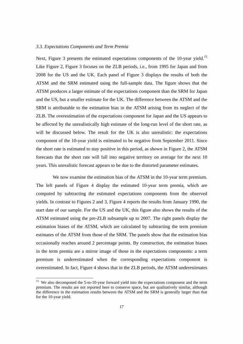
Next, Figure 3 presents the estimated expectations components of the 10-year yield.15

Like Figure 2, Figure 3 focuses on the ZLB periods, i.e., from 1995 for Japan and from

2008 for the US and the UK. Each panel of Figure 3 displays the results of both the

ATSM and the SRM estimated using the full-sample data. The figure shows that the

ATSM produces a larger estimate of the expectations component than the SRM for Japan

and the US, but a smaller estimate for the UK. The difference between the ATSM and the

SRM is attributable to the estimation bias in the ATSM arising from its neglect of the

ZLB. The overestimation of the expectations component for Japan and the US appears to

be affected by the unrealistically high estimate of the long-run level of the short rate, as

will be discussed below. The result for the UK is also unrealistic: the expectations

component of the 10-year yield is estimated to be negative from September 2011. Since

the short rate is estimated to stay positive in this period, as shown in Figure 2, the ATSM

forecasts that the short rate will fall into negative territory on average for the next 10

years. This unrealistic forecast appears to be due to the distorted parameter estimates.

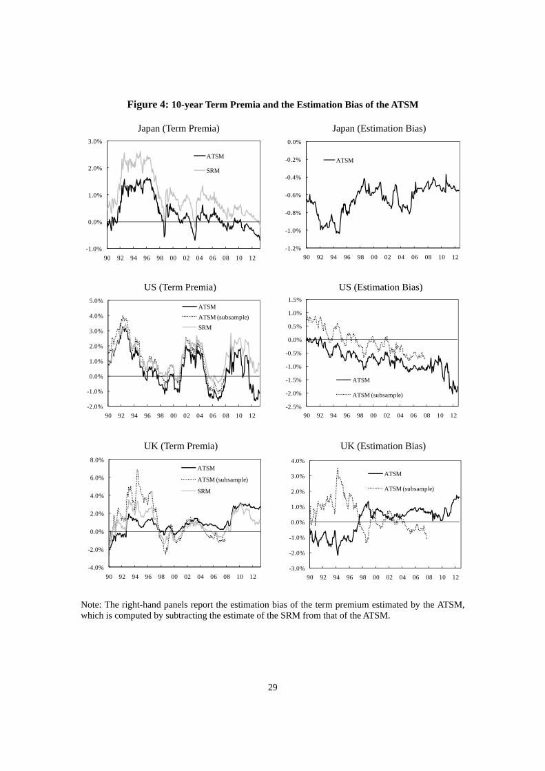
We now examine the estimation bias of the ATSM in the 10-year term premium.

The left panels of Figure 4 display the estimated 10-year term premia, which are

computed by subtracting the estimated expectations components from the observed

yields. In contrast to Figures 2 and 3, Figure 4 reports the results from January 1990, the

start date of our sample. For the US and the UK, this figure also shows the results of the

ATSM estimated using the pre-ZLB subsample up to 2007. The right panels display the

estimation biases of the ATSM, which are calculated by subtracting the term premium

estimates of the ATSM from those of the SRM. The panels show that the estimation bias

occasionally reaches around 2 percentage points. By construction, the estimation biases

in the term premia are a mirror image of those in the expectations components: a term

premium is underestimated when the corresponding expectations component is

overestimated. In fact, Figure 4 shows that in the ZLB periods, the ATSM underestimates

15 We also decomposed the 5-to-10-year forward yield into the expectations component and the term premium. The results are not reported here to conserve space, but are qualitatively similar, although the difference in the estimation results between the ATSM and the SRM is generally larger than that for the 10-year yield.

18

the term premium for Japan and the US, while it overestimates that for the UK. As can

also be seen, the estimation bias for the US and the UK increases for the most recent

years. In the pre-ZLB periods, the ATSM at least for Japan and the US tends to

underestimate the term premium, when the full sample is used to estimate the ATSM. For

the UK, although the ATSM overestimates the term premium in the 2000s, it

considerably underestimates the premium in the 1990s. When the pre-ZLB subsample is

used, however, no clear systematic underestimation of the term premia is any longer

detected.

The reasons behind the biased estimates of the expectations components and the

term premia are difficult to identify. This is because the parameter and factor estimates

are distorted to mitigate the original problem of ATSMs, which generates new problems.

By their nature, ATSMs produce biased expected values of future short-term interest rates

under both the P- and Q-measures, for the following two reasons. First, ATSMs forecast

a negative short rate with positive probability, which leads to an underestimation of the

expectations components. Second, at the ZLB, ATSMs forecast that the short rate will

start to rise immediately, which contributes to an overestimation of the expectations

components. The relative importance of these opposite effects depends on the parameters

and the factors. The biased expected values under the P-measure lead to the biased

decomposition of yields between expectations components and term premia. The biased

expected values under the Q-measure lead to biased model-implied yields. To reduce the

fitting errors arising from the problematic nature of ATSMs, the estimates of the

parameters and the factors are also biased. The different characteristics of the estimation

bias of the ATSM across the three countries and the two sample periods suggest that how

the problematic nature of the ATSM and the estimation bias of the parameters and factors

interact with each other depends on the properties of the data.

Despite the complexity of the sources of the estimation bias in the ATSM, there is

one consistent result: the ATSM overestimates the long-run level of the short rate, as

discussed in Subsection 3.1. This appears to result in the tendency of the ATSM to

underestimate the term premium. This relationship between the overestimation of the

long-run level and the underestimation of the term premium is supported by the

19

observation that both the systematic underestimation of the term premium and the

overestimation of the long-run level of the short rate are less clear when the pre-ZLB

subsample is used to estimate the ATSM.

4. Conclusion

Studies such as Ichiue and Ueno (2006, 2007, 2012) simultaneously take into account

time-series and cross-sectional variation in the data to estimate SRMs using Japan’s yield

data during its low interest rate environment from 1995 onward. This paper estimates an

SRM using not only Japanese data but also US and UK data from 1990 onward – a

period that includes both periods of low and high interest rates. By comparing the results

of the SRM with those of an ATSM, we examine how the fact that ATSMs neglect the

ZLB produces biased estimates.

We find that the ATSM and the SRM produce very different estimates, which are

attributable to the estimation bias of the ATSM. The ATSM often produces unrealistic

results such as an unreasonably high long-run level of the short rate and a negative

expectations component of the 10-year yield. The 10-year term premium estimated by the

ATSM occasionally deviates from that estimated by the SRM by around 2 percentage

points, and the deviation has recently widened in the US and the UK. The ATSM

consistently overestimates the long-run level of the short rate, which appears to

contribute to the tendency to underestimate the term premium. Using the pre-ZLB

subsample up to 2007 for the US and UK diminishes the systematic underestimation of

the term premium, which suggests that the ZLB sample distorts the estimation results of

the ATSM to a considerable extent.

In all three countries examined here – Japan, the US, and the UK – the

respective central banks have now maintained near-zero policy rates for more than four

years. In addition, the ZLB environment is expected to last for at least a few more years.

Further, even after central banks start raising their policy rates, researchers will need to

use time-series data from periods at or near the ZLB to ensure a sufficient number of

observations for reliable empirical exercises. Therefore, researchers will have to keep

20

struggling with the ZLB perhaps for at least the next decade. This paper is merely one

step toward understanding how the ZLB changes the relevance of the models that were

useful at one time. Further research on term structure models that take the ZLB into

account is needed. At the same time, the previous results obtained based on models

which do not account for the ZLB should be reexamined. A possible direction for future

research is to estimate an SRM by additionally using data on inflation-indexed bond

yields to extract bond market participants’ inflation expectations, as D’Amico et al.

(2010) do using an ATSM.

21

References

Ahn, D., R. F. Dittmar, and A. R. Gallant (2002), “Quadratic Term Structure Models: Theory and Evidence,” Review of Financial Studies 15, 243-288.

Bauer, M. D. and C. J. Neely (2012), “International Channels of the Fed’s Unconventional Monetary Policy,” Federal Reserve Bank of San Francisco Working Paper Series 2012-12.

Bauer, M. D. and G. D. Rudebusch (2011), “The Signaling Channel for Federal Reserve Bond Purchases,” Federal Reserve Bank of San Francisco Working Paper Series 2011-21.

Bernanke, B. (2013), “Long-term Interest Rates,” Remarks at the Annual Monetary/Macroeconomic Conference: The Past and Future of Monetary Policy Sponsored by Federal Reserve Bank of San Francisco, San Francisco, California, March 1, 2013.

Black, F. (1995), “Interest Rates as Options,” Journal of Finance 50, 1371-1376.

Christensen, J. H. E. and G. D. Rudebusch (2012), “The Response of Interest Rates to U.S. and U.K. Quantitative Easing,” Economic Journal 122, 385-414.

Christensen, J. H. E. and G. D. Rudebusch (2013), “Estimating Shadow-Rate Term Structure Models with Near-Zero Yields,” Federal Reserve Bank of San Francisco Working Paper Series 2013-07.

Chung, H., J.-P. Laforte, D. Reifschneider, and J. C. Williams (2012), “Have We Underestimated the Likelihood and Severity of Zero Lower Bound Events?” Journal of Money, Credit and Banking 44, 47-82.

Cox, J., J. Ingersoll, and S. Ross (1985), “A Theory of the Term Structure of Interest Rates,” Econometrica 53, 385-407.

Dai, Q. and K. J. Singleton (2000), “Specification Analysis of Affine Term Structure Models,” Journal of Finance 55, 1943-1978.

D’Amico, S., W. English, D. Lopez-Salido, and E. Nelson (2012), “The Federal Reserve’s Large-scale Asset Purchase Programmes: Rationale and Effects,” Economic Journal 122, 415-446.

D’Amico, S., D. H. Kim, and M. Wei (2010), “Tips from TIPS: The Informational Content of Treasury Inflation Protected Security Prices,” Federal Reserve Board Finance and Economics Discussion Series 2010-19.

de Jong, F. (2000), “Time Series and Cross-section Information in Affine Term-Structure Models,” Journal of Business & Economic Statistics 18, 300-314.

Duffie, D. (2001), Dynamic Asset Pricing Theory, third edition, Princeton University Press.

22

Duffie, D. and R. Kan (1996), “A Yield-factor Model of Interest Rates,” Mathematical Finance 6, 379-406.

Gagnon, J., M. Raskin, J. Remache, and B. Sack (2011), “The Financial Market Effects of the Federal Reserve’s Large-Scale Asset Purchases,” International Journal of Central Banking 7, 3-43.

Gorovoi, V. and V. Linetsky (2004), “Black’s Model of Interest Rates as Options, Eigenfunction Expansions and Japanese Interest Rates,” Mathematical Finance 14, 49-78.

Gürkaynak, R. S., B. Sack, and J. Wright (2007), “The U.S. Treasury Yield Curve: 1961 to the Present,” Journal of Monetary Economics 54, 2291-2304.

Hamilton, J. D. and J. C. Wu (2012), “The Effectiveness of Alternative Monetary Policy Tools in a Zero Lower Bound Environment,” Journal of Money, Credit and Banking 44, 3-46.

Ichiue, H. and Y. Ueno (2006), “Monetary Policy and the Yield Curve at Zero Interest: The Macro-finance Model of Interest Rates as Options,” Bank of Japan Working Paper Series 06-E-14.

Ichiue, H. and Y. Ueno (2007), “Equilibrium Interest Rate and the Yield Curve in a Low Interest Rate Environment,” Bank of Japan Working Paper Series 07-E-18.

Ichiue, H. and Y. Ueno (2012), “Monetary Policy and the Yield Curve at Zero Interest,” mimeo.

Ihrig, J., E. Klee, C. Li, B. Schulte, and M. Wei (2012), “Expectations about the Federal Reserve’s Balance Sheet and the Term Structure of Interest Rates,” Federal Reserve Board Finance and Economics Discussion Series 2012-57.

Joyce, M., P. Lildholdt, and S. Sorensen (2010), “Extracting Inflation Expectations and Inflation Risk Premia from the Term Structure: A Joint Model of the UK Nominal and Real Yield Curves,” Journal of Banking and Finance 34, 281-294.

Joyce, M., M. Tong, and R. Woods (2011), “The United Kingdom's Quantitative Easing Policy: Design, Operation and Impact,” Bank of England Quarterly Bulletin, 2011, 3rd Quarter, 200-212.

Kikuchi, K. (2012), “Design and Estimation of a Quadratic Term Structure Model with a Mixture of Normal Distributions,” Bank of Japan IMES Discussion Paper Series 2012-E-8.

Kim, D. H. and K. J. Singleton (2012), “Term Structure Models and the Zero Bound: An Empirical Investigation of Japanese Yields,” Journal of Econometrics 170, 32-49.

Kim, D. H. and J. H. Wright (2005), “An Arbitrage-free Three-factor Term Structure Model and the Recent Behavior of Long-term Yields and Distant-horizon Forward Rates,” Federal Reserve Board Finance and Economics Discussion Series 2005-33.

23

Koeda, J. (2012), “Endogenous Monetary Policy Shifts and the Term Structure: Evidence from Japanese Government Bond Yields,” CARF Working Paper CARF-F-303.

Krippner, L. (2012a), “Modifying Gaussian Term Structure Models when Interest Rates Are near the Zero Lower Bound,” Reserve Bank of New Zealand Discussion Paper 2012/02.

Krippner, L. (2012b), “Measuring the Stance of Monetary Policy in Zero Lower Bound Environments,” Reserve Bank of New Zealand Discussion Paper 2012/04.

Leippold, M. and L. Wu (2003), “Design and Estimation of Quadratic Term Structure Models,” European Financial Review 7, 47-73.

Li, C. and M. Wei (2013), “Term Structure Modelling with Supply Factors and the Federal Reserve’s Large-scale Asset Purchase Programs,” International Journal of Central Banking 9, 3-44.

McCulloch, R. (1990), “U.S. Government Term Structure Data, 1947-1987,” in B. M. Friedman and F. Hahn, eds., Handbook of Monetary Economics, North Holland I, 672-715.

Ueno, Y., N. Baba, and Y. Sakurai (2006), “The Use of the Black Model of Interest Rates as Options for Monitoring the JGB Market Expectations,” Bank of Japan Working Paper Series 06-E-15.

24

Table 1: Estimated Standard Deviations of the Fitting Errors , (in Basis Points)

Japan US UK

SRM -2012

ATSM -2012

SRM -2012

ATSM -2012

ATSM -2007

SRM -2012

ATSM -2012

ATSM -2007

Policy rate 44 45 67 66 70 90 70 75

0.5y or 1y 1 0 13 15 13 22 0 0

2y 11 10 0 0 0 2 14 12

5y 15 4 4 0 0 5 0 0

10y 8 21 11 12 10 24 33 26

Note: “0.5y or 1y” reports the standard deviation of the 0.5-year yield for Japan, and that of the 1-year yield for the US and the UK.

25

Table 2: Parameter Estimates

Japan US UK

SRM -2012

ATSM -2012

SRM -2012

ATSM-2012

ATSM-2007

SRM -2012

ATSM -2012

ATSM-2007

-0.0266 -0.0622 -0.0566 -0.0741 -0.0602 -0.0305 -0.0906 -0.0511

-0.0358 -0.1397 -0.0764 -0.1029 -0.1123 -0.0388 -0.3080 -0.0501

-0.0173 -0.0204 -0.0024 -0.0444 -0.1047 -0.0061 -0.5318 -0.1783

-0.0576 -0.0215 -0.0168 -0.1718 -0.2118 -0.0141 -0.0154 -0.1262

-0.0081 -0.0042 -0.0106 -0.0088 -0.0067 -0.0143 -0.0051 -0.0095

-0.0036 -0.0047 -0.0061 -0.0068 -0.0080 -0.0075 -0.0114 -0.0099

-0.0002 -0.0001 0.0000 -0.2469 -0.3146 -0.0002 --0.0265 -0.0060

-0.0008 0.0001 -0.0001 -0.0230 -0.0061 -0.0004 -0.0087 -0.0518

-0.2481 -0.2699 -0.4888 -0.3059 -0.3260 -0.4661 -0.0522 -0.6268

-0.3775 -0.2872 -0.6371 -0.1820 -0.4010 -0.4676 -0.7801 -0.6478

-0.1279 -0.2465 -0.2428 -0.3750 -0.1813 -0.1037 -0.0193 -0.0020

-0.2030 -0.1248 -0.2519 -0.2173 -0.2691 -0.0948 -0.1296 -0.1276

Max eig 0.9970 0.9982 0.9986 0.9915 0.9907 0.9988 0.9987 0.9958

Max eig 0.9943 0.9873 0.9927 0.9850 0.9915 0.9985 0.9950 1.0000

Note: The last two rows report the largest modulus of the eigenvalues of the estimated and .

26

Figure 1: Selected Yield Data

Japan

US

UK

0%

1%

2%

3%

4%

5%

6%

7%

8%

9%

90 92 94 96 98 00 02 04 06 08 10 12

10y yield

2y yield

Policy rate

0%

1%

2%

3%

4%

5%

6%

7%

8%

9%

10%

90 92 94 96 98 00 02 04 06 08 10 12

10y yield

2y yield

Policy rate

0%

2%

4%

6%

8%

10%

12%

14%

16%

90 92 94 96 98 00 02 04 06 08 10 12

10y yield

2y yield

Policy rate

27

Figure 2: The Short Rate of the ATSM and the Shadow Rate of the SRM

Japan

US

UK

-2.0%

-1.5%

-1.0%

-0.5%

0.0%

0.5%

1.0%

1.5%

2.0%

2.5%

95 97 99 01 03 05 07 09 11 13

ATSM spot rate

SRM shadow rate

-3.0%

-2.5%

-2.0%

-1.5%

-1.0%

-0.5%

0.0%

0.5%

1.0%

1.5%

2.0%

2.5%

08 09 10 11 12 13

ATSM spot rate

SRM shadow rate

-4.0%

-3.0%

-2.0%

-1.0%

0.0%

1.0%

2.0%

3.0%

4.0%

5.0%

6.0%

08 09 10 11 12 13

ATSM spot rate

SRM shadow rate

28

Figure 3: Expectations Components of the 10-year Yield

Japan

US

UK

0%

1%

2%

3%

4%

95 97 99 01 03 05 07 09 11 13

ATSM

SRM

0%

1%

2%

3%

4%

5%

08 09 10 11 12 13

ATSM

SRM

-2%

-1%

0%

1%

2%

3%

4%

5%

6%

08 09 10 11 12 13

ATSM

SRM

29

Figure 4: 10-year Term Premia and the Estimation Bias of the ATSM

Japan (Term Premia) Japan (Estimation Bias)

US (Term Premia) US (Estimation Bias)

UK (Term Premia) UK (Estimation Bias) Note: The right-hand panels report the estimation bias of the term premium estimated by the ATSM, which is computed by subtracting the estimate of the SRM from that of the ATSM.

-1.0%

0.0%

1.0%

2.0%

3.0%

90 92 94 96 98 00 02 04 06 08 10 12

ATSM

SRM

-2.0%

-1.0%

0.0%

1.0%

2.0%

3.0%

4.0%

5.0%

90 92 94 96 98 00 02 04 06 08 10 12

ATSM

ATSM (subsample)

SRM

-4.0%

-2.0%

0.0%

2.0%

4.0%

6.0%

8.0%

90 92 94 96 98 00 02 04 06 08 10 12

ATSM

ATSM (subsample)

SRM

-1.2%

-1.0%

-0.8%

-0.6%

-0.4%

-0.2%

0.0%

90 92 94 96 98 00 02 04 06 08 10 12

ATSM

-3.0%

-2.0%

-1.0%

0.0%

1.0%

2.0%

3.0%

4.0%

90 92 94 96 98 00 02 04 06 08 10 12

ATSM

ATSM (subsample)

-2.5%

-2.0%

-1.5%

-1.0%

-0.5%

0.0%

0.5%

1.0%

1.5%

90 92 94 96 98 00 02 04 06 08 10 12

ATSM

ATSM (subsample)