estimating the cost structure of the local telephone...
TRANSCRIPT

ESTIMATING THE COST STRUCTURE OF THE LOCAL TELEPHONE EXCHANGE NE1WORK
prepared for the
NATIONAL REGULATORY RESEARCH INSTITUTE The Ohio State University
1080 Carmack Road Columbus, Ohio 43210
by
David Gabel Queens College
and
Mark Kennet Tulane University
October 1991
NRRI 91-16
This report was prepared for The National Regulatory Research Institute (NRRI) with funding provided by participating member commissions of the National Association of Regulatory Utility Commissioners (NARUC). The views and opinions of the authors do not necessarily state or reflect the views, opinions, or policies of the NRRI, the NARUC, or NARUC member commissions.

j
j
j
j
j
j
j
j
j
j
j
j
j
j
j
j
j
j
j
j
j
j
j
j
j
j
j
j
j
j
j
j
j
j
j
j
j
j
j
j
j
j
j
Executive Summary
Effective regulation requires a thorough understanding of the cost structure of the
industry. Costs serve as a basis for judging the reasonableness of rates, and provide an
indication of the extent to which an industry is a natural monopoly.
Regulatorj COll1111issions have lacked an analytical tool that permitted them to
independently quantify the cost of different services. Instead, information regarding the
cost structure of the industry has largely come from telephone company-sponsored cost
studies. While the companies' cost studies provided valuable insights into many issues,
we felt that Commissions would benefit from having in-hand their own analytical tool
that could provide an aid in analyzing such issues as the cost of exchange services, the
economics of bypass and fiber optics in the local telecommunications network, and the
extent to which the industry is a natural monopoly.
The attached report describes the operation of the cost model as well as our
findings. We have concluded that the replacement of analog with digital technology has
lowered the marginal cost of providing switched exchange and toll services and has
raised the marginal cost of providing switched access and private line services. The
reduction in the cost of providing switched services is largely due to the savings in
interoffice transport costs. Switched access costs have increased in large part because
many of the functions that were previously handled by the central processor unit of the
switching machine, as well as other peripheral equipment, are now handled by customer .
specific equipment. Private line costs have increased, in part, because of the
replacement of analog copper with digital trunks, and because these services no longer
share the fixed cost of interoffice channel banks with switched services.
Based on our analysis of the stand-alone cost of constructing private line systems,
we have found that in densely populated markets, it is possible for an entrant to .provide
private line services at a lower cost than the local exchange telephone companies. The
entrant, unlike the incumbent telephone companies, chooses to provide all services
through one central office. This provides an important cost saving on interoffice
111
trunking. Consequently, bypass can occur not because of the commonly alleged
regulatory inefficiencies, but because an entrant can provide service at a lower cost than
the local exchange telephone company.
In less densely populated markets, an entrant can not provide service at a lower
cost than the local exchange company. Because of the cost of placing cables over a wide
geographical area, society's costs are minimized when all services are provided by one
firm.
In order for an industry to be a natural monopoly, it must be cheaper for one firm
to provide all services than to have two or more firms provide the same products. We
have found that while in general the industry may be a natural monopoly, in densely
populated markets the telecommunications industry is not a natural monopoly. The
provision of private line services by one firm, and switched services by a second firm,
leads to a reduction in the total cost of production.
The finding that the industry is not always a natural monopoly has important
regulatory implications. The history of the industry indicates that there is a strong need
for regulatory oversight in order to ensure that services subject to competition are not
subsidized by monopoly services.
The output from the cost model also indicates that fiber optics in the local loop is
not the cost minimizing technology. On short loops, copper cable is still the cost
minimizing technology. On longer loops, copper is more expensive than digitally derived
loops using subscriber-line carrier. Subscriber-line carrier on copper is 8 to 16 percent
cheaper than subscriber-line carrier on fiber. This comparison is based on the
assumption that the telephone company deploys a small fiber cable (one that satisfies the
level of demand). In practice local exchange companies often install fiber cables with a
large amount of excess capacity (dark fiber). When this extra capacity is installed, the
cost of fiber in the loop is increased and this makes subscriber-line carrier on fiber
significantly more expensive than suggested by the data developed in this report. The
cost difference between subscriber-line carrier on copper and fiber is not large, and
because of the greater bandwidth available on fiber, telephone companies are willing to
incur the additional cost associated with fiber. As with the other technologies that
lV

improve the provision of data and enhanced services at the cost of raising access to the
public switched network (for example, digital switching), we believe that these costs
should not be borne exclusively by customers of plain-old-telephone-service.
v


TABLE OF CONTENTS
LIST OF FIGURES .............................................. x UST OF TABLES. . . . . . . . . . . . . . . . . . . . . . . . . . . . . . . . . . . . . . . . . . . . .. xi FOREWORD ............................................... XlII
ACKNOWLEDGEMENTS ....................................... xv
Chapter Page
1 An Overview of Previous Cost Studies ............................ 1
Modeling Advantages Associated with LECOM .................. 4 Minimizing the Cost of Service . . . . . . . . . . . . . . . . . . . . . . . . . . .. 5 Evaluation of Alternative Technologies . . . . . . . . . . . . . . . . . . . . .. 6 Output Mix .......................................... 6 Technological Change . . . . . . . . . . . . . . . . . . . . . . . . . . . . . . . . . .. 7 Fixed and Variable Costs of Production ..................... 9
Modeling Disadvantages Associated with LECOM .0 •••••••••••••• 10 Administrative Costs ....................... 0 • • • • • • • • • • • • 10 Bounded Rationality .................................... 11
A Preview of Remaining Chapters ............................ 12
2 Telephone Network Facilities ................................... 15
I. Introduction............................................. 15 II. Network Topology ........................................ 15
Local Loop Topology . . . . . . . . . . . . . . . . . . . . . . . . . . . . . . . . . . . . . . 17 The Local Loop: Copper Wires in the Analog Network ............. 20 Installed Capacity in the Local Loop . . . . . . . . . . . . . . . . . . . . . . . . . . . 21 Placing the Cable Underground ............................. . New Technology in the Local Loop ........................... 23
Subscriber Line Carrier ............................... .. 24 Remotes ............................................. 27
Switch Deployment ........................................ 27 Toll Office .............................................. 30 Interoffice Traffic . . . . . . . . . . . . . . . . . . . . . . . . . . . . . . . . . . . . . . . . . 31 Customer Density ......................................... 32
III. Assumptions (A) and Definitions (D) in the Model .... 0 ••••••••••• 34 General Program Description . . . . . . . . . . . . . . . . . . . . . . . . . . . . . . . . Whose Costs Are Being Modeled? ............................ 40
IV. Cost of the Technologies ................................... 43 Cost Structure of the Local Loop ............................. 43
vii

TABLE OF CONTENTS (Continued)
2
Fiber Optics . . . . . . . . . . . . . . . . . . . . . . . . . . . . . . . . . . . . . . . . . . . . . 47 The Cost of Interoffice Calls . . . . . . . . . . . . . . . . . . . . . . . . . . . . . . . . . 48 Private-line Costs ........................................ 49 Switching Costs .......................................... 50 Input Prices ............................................. 50 User Inputs ............................................. 51
3 Methodology for Generating Data ............................... 53
Optimization ............................................ 53 Generating Data ......................................... 54
4 Cost Estimates .............................................. 57
Discussion of Econometric Results ............................ 57 Directly Estimating the Incremental Cost of Service ............... 59 Why Might the Loop Length Increase When the Number of Switches Deployed Increases? ............................... 68
Is the Local Exchange Market a Natural Monopoly? ............... 69 If the Industry is Not a Natural Monopoly, What Does This Imply About the Need to Regulate the Industry .............. 80
5 Additional Analysis of the Cost of Service ......................... 81
The Economics of Fiber Optics .............................. 81 Fiber Optics on Interoffice Trunks ............................ 81 Fiber Optics in the Local Loop . . . . . . . . . . . . . . . . . . . . . . . . . . . . . . . 82 Pricing ................................................ 83
6 Conclusion and Some Future Uses for the Model .................... 89
APPENDIX ONE: Econometric Results .............................. 93 Using the Model to Calculate the Marginal Cost of Service .......... e . 106 Lumpy Investments and Discountinuities .......................... 109
APPENDIX TWO: LECOM Manual ............................ e .. 113 Ie Introduction................................................ 113 II. Getting Started ............................................ 115 III. Editing Data Files .......................................... 117 IV. Operating the Programs ...................................... 121
Vlll
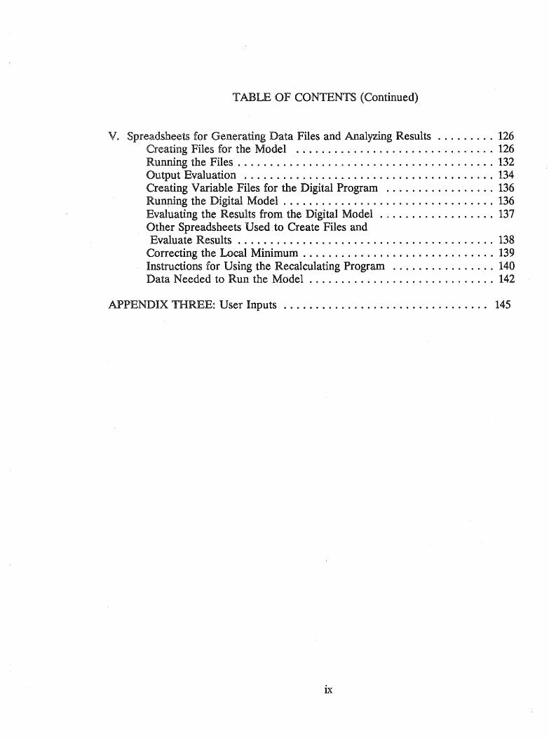
TABLE OF CONTENTS (Continued)
v. Spreadsheets for Generating Data Files and Analyzing Results ......... 126 Creating Files for the Model ............................... 126 Running the Files . . . . . . . . . . . . . . . . . . . . . . . . . . . . . . . . . . . . . . . . 132 Output Evaluation ....................................... 134 Creating Variable Files for the Digital Program ................. 136 Running the Digital Model . . . . . . . . . . . . . . . . . . . . . . . . . . . . . . . . . 136 Evaluating the Results from the Digital Model .................. 137 Other Spreadsheets Used .to Create Files and Evaluate Results . . . . . . . . . . . . . . . . . . . . . . . . . . . . . . . . . . . . . . . . 138
Correcting the Local Minimum ................. 0 •••••••••• 0 0 139 Instructions for Using the Recalculating Program ..... 0 • • • 0 0 • • • 0 • 140 Data Needed to Run the Model ... 0 0 •••••••••••••••••••••••• 142
APPENDIX THREE: User Inputs . 0 • 0 •••••• 0 •••• 0 .0 ••••• 0 0 •• 0 • • •• 145
ix
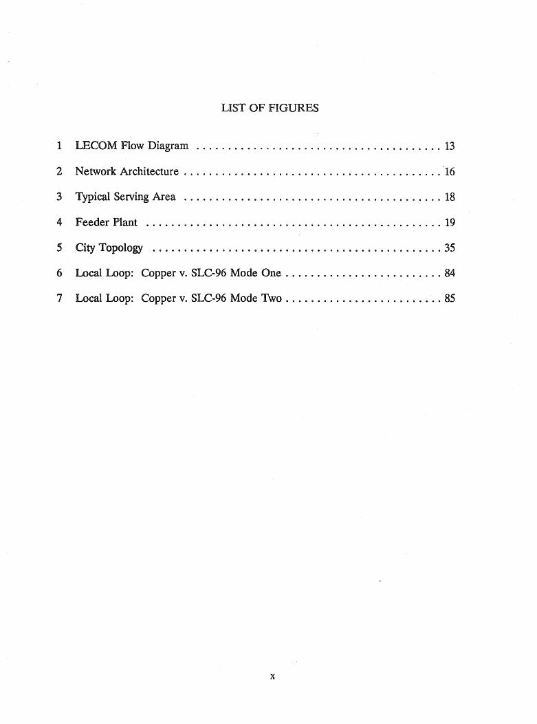
LIST OF FIGURES
1 LECOM Flow Diagram ....................................... 13
2 Network Architecture ......................................... "16
3 Typical Serving Area ......................................... 18
4 Feeder Plant ............................................... 19
5 City Topology .............................................. 35
6 Local Loop: Copper v. SLC-96 Mode One ......................... 84
7 Local Loop: Copper v. SLC-96 Mode Two ......................... 85
x

LIST OF TABLES
Feeder and Distribution Pairs Per Customer ......................... 0 • 22
Cost Trade Off: Large v. Small Switches .............................. 29
Intraoffice Calls: Proportion of Total Calls . . . . . . . . . . . . . . . . . . . . • . . . . . . . 31
Subscriber Densities in Selected Cities ................. .. 0 • • • 0 • • •• 0 • • 33
1987 Investment Per Drop Line: Business v. Residential .................. 47
Fiber Multiplexers ..... 0 ••••••• 0 •••••••• 0 ••• 0 ••••••••••••••••••• 47
LECOM User Inputs .................................. o .••••••••• 52
Combinations Ran in Generating Data ................... 0 ••••••••••• 55
Marginal Cost of Service ......................................... 61
Diseconomies of Scope: Analog Network ............................. 72
Diseconomies of Scope: Digital Network ............................. 74
Economies of Scope: Analog Network ................. 0 ••••••••••••• 78
Economies of Scope: Digital Network ................................ 79
Impact of Digital Technology on the Annual Cost of Providing Access and Exchange Services .................................... 87
Variable Mnemonics ............................................ 95
Translog Estimation Results ....................................... 96
Homogeneity Experiment Results ................................... 99
Analog Translog Estimates With Interaction Terms Removed ............. 101
Translog Estimates With Access Lines Not Treated as a Product ... 0 •••••• 103
Mean Values and Standard Deviations for Variables Used ............... 106
Xl
UST OF TABLES (Continued)
Results from Two Runs of the Simulation Model ...................... 107
Using the Translog Parameters to Estimate the Cost of Service ............ 108
Variations in the Incremental Cost of Service . . . . . . . . . . . . . . . . . . . . . . . . . 111
Creating Files .. . . . . . . . . . . . . . . . . . . . . . . . . . . . . . . . . . . . . . . . . . . . . . 128
Spreadsheet With Outputs Summarized ............................. 135
List of Spreadsheets . . . . . . . . . . . . . . . . . . . . . . . . . . . . . . . . . . . . . . . . . . . . 139
Information Requests and Variable Names ........................... 144
xii

Foreword
From time to time the NRRI funds a study by an "outside" researcher on a topic
likely to be of interest to our clientele as part of our Occasional Paper series .. We view
this series as something like a technical journal and as such a fairly specialized
knowledge of the subject matter is usually helpful for a full understanding of the analysis.
In this Occasional Paper the facult'j authors have devised and tested a costing tool
for allowing commissions to analyze issues such as the real cost of exchange services, the
economics of bypass, and the extent to which the industry is a natural monopoly. One
copy of the software has been transmitted to the chair of each commission. Copies may
also be obtained by contacting the authors.
We hope commission staff find this a useful contribution.
xiii
Douglas N. Jones Director, NRRI Columbus, Ohio October 1, 1991

1
1
1
1
1
1
1
1
1
1
1
1
1
1
1
1
1
1
1
1
1
1
1
1
1
1
1
1
1
1
1
1
1
1
1
1
1
1
1
1
1
1
1
1
1
1
1
1
1
1
1
1
1
1
1
1
1
1
1
1
1
1
1
1
1
1
1
1
1
1
1
1
1
1
1
1
1
1
1
1
1
1
1
1
1
1
1
1
1
1
1
1
1
1
1
1
1

Acknowledgements
Many people provided invaluable support for this project. Doug Jones, Ray
Lawton and Bill Pollard of NRRI expressed strong initial interest in our proposal and
have provided helpful suggestions along the way. In addition, they provided us with
important forums for sharing and exchanging ideas with others.
Many individuals helped us obtain data for this project. Some of our primary
benefactors (but by no means an exhaustive list) were David Gebhardt Jr., (Illinois Bell
Telephone Company), John Nestor III (New England Telephone Company), Pat
Gardzella (New York Telephone), Viktor Schmid-Bielenberg (Bellcore), F.D. D'Alessio
(New Jersey Telephone Company), Paul Polishuk (Information Gatekeepers), Robert
Bowman (U.S. West), Susan Baldwin (Massachusetts Department of Public Utilities),
Dale Lundy (Southwestern Telephone Company), Raymond Hayden Jr. (Rural Electrical
Administration), Dan Dunbeck (Rural Electrical Administration) and Bruce Gallagher
(New Jersey Board of Public Utilities).
This work was made possible in part by research computing facilities provided by
the City University of New York and Tulane University. Ed Greenman and Sal Saieva
provided us with invaluable computer assistance.

CHAPTER ONE
AN OVERVIEW OF PREVIOUS COST STUDIES
Since 1960 the cost function of the telecommunications industry has been studied
extensively, the initial work coinciding with the introduction of microwave facilities. This
mode of long-distance transmission made it possible for firms to establish networks that
could compete with American Telephorte at,d Telegraph Company's (AT&T) long=
distance lines.
Responding to this entry, AT&T offered large business customers significant price
discounts for bulk private line service. Since then, state and federal regulatory
commissions have sought a sound economic method to evaluate the reasonableness of
rates.
Three costing methods have emerged over this time period each having various
strengths and weaknesses. The methods are: 1) accounting, 2) engineering, and 3)
statistical studies. This report off~rs an alternative modelling approach combining
engineering process modelling, optimization techniques, and statistical estimation.
Accounting data have been used to determine the embedded cost of service in
virtually every jurisdiction in the United States. The advantage of this type of analysis is
that the same data are used to determine the firm's revenue requirement; therefore, it is
readily available. Its primary drawback is that it is of limited value in indicating the
future economic costs that the utility will incur. For economic efficiency, rates should
reflect forward looking, or opportunity, cost of service.
Telephone companies have generally argued that setting rates should be based on
prospective costs. Economic theory stresses that to maximize society's welfare, prices
should reflect the forward looking marginal cost of production. To support tariff changes
telephone companies often submit long-run incremental cost studies (LRIC).
Based upon engineering production rules, the LRIC studies identify the cost of
increasing output on only one component of the network, such as a switch or a loop.
The LRIC studies are not designed to quantify the total cost of service (that is, the total
1

cost, both variable and fixed, of providing multiple services), however, the total cost of
service is important for decisions regarding entry into the industry. The restructuring of
AT &Tl as well as federal and state commission proposals to allow entry into the
industry can be characterized as "beneficial" or "harmful" in part depending on the extent
to which the industry is a natural monopoly. This, as wen as the degree of economies of
scale and scope, can only be measured by having information about the total cost curve.2
In recent years participants in regulatory and judicial proceedings have presented
statistical estimateS of the industr/s total cost CllI"'{e. "'bile an important innovation,
these studies had significant limitations due to the quality of the data.
Starting with historical data, econometricians encountered the problem of how to
control for technological change. While proxies such as research and development
expenditures or the number of access lines served by electronic switching machines have
been used, they only roughly capture the impact of technological change.
Researchers also had trouble controlling for input prices and constructing output
indexes for the various categories of service. Because of these and other data problems,
Evans and Heckman have argued that before conclusive statements about the cost
function can be made, new data would have to be located.3
This research attempts to address these data problems by combining engineering
process models with optimization techniques to estimate the cost of local exchange
facilities. The model, LECOM (local exchange cost optimization model) was created by
first developing algorithms that incorporate the engineering standards and practices used
lUnited States v. American Tel. & Tel. Co., 552 F. SUppa 131 (D.D.C. 1982) affd sub nom. Maryland v United States, 460 U.S. 1001 (1983).
2William W. Sharkey, The Theory of Natural Monopoly (Cambridge, MA: Cambridge University Press, 1982).
3See, for example, Leonard Waverman, "U.S. Interexchange Competition," in Robert Crandall and Kenneth Flamm, Changing the Rules: Technological Change, International Competition, and Regulation in the Communications Industry (Washington: Brookings Institute, 1988); and D.S. Evans and 1.1. Heckman, "Rejoinder: Natural Monopoly and the Bell System: Response to Charnes, Cooper and Sueyoshi, " Management Science 34 no. 27: 37 (1988).
2

by telephone company engineers for designing local exchange networks (that is, a process
model). Second, the cost-output relationship is derived as a result of assumed
optimization behavior. Here the minimum cost of production is identified for various
output levels given input prices and the production function. LECOM was designed to
search for the combination and location of switching machines that minimize the cost of
production.4
Through repeated simulations of the cost-output relationship, we were able to
develop a data base that helps us measure the cost impact of varying the level of output
of various services. The cost data generated by LECOM is summarized through a
statistical estimate of the cost function.5
For policy analysis, this method of generating data offers an important advantage
compared to the data used by earlier econometricians. Much of the research interest in
the industry's cost structure is tied to a concern about the efficiency of entry and
competition. Most of the published work has been based on data from the Bell
Operating Companies, each of which provides service in many cities. The level of
observation is therefore the firm, not a market, such as for a city. Entry, on the other
hand, often occurs at the city level. Entrepreneurial firms, such as Teleport, do not
provide statewide operations, but instead offer just service in the most profitable
markets.
~is is a departure from the methodology used by most telephone companies. By searching for the combination and location of switching machines, the model is implicitly unconstrained by prior investment decisions. Typically telephone company cost studies assume that the number and location of telephone switches is fixed.
5Summarizing the output from a process model through the use of a statistical cost function, has been used in other industry studies. See, for example, James M. Griffen, liThe Process Analysis Alternative to Statistical Cost Functions," American Economic Review 62 (Mar .. 1972): 46-56; Alan Manne, "A Linear Programming Model of the U.S. Petroleum Refining Industry," Econometrica 26 (Jan. 1958): 67-106; Hollis B. Chenery, "Engineering Production Functions," Quarlerly Journal of Economics 43: 507-31; and James M. Griffen, "Long-run Production Modeling with Pseudo Data: Electric Power Generation," Bell Journal of Economics 8 (Spring 1977): 112-27.
3
To understand the economic rationale of entry a comparison between the
operations of an incumbent and an entrant at the market level is of some value. Little
insight is gained by comparing the statewide operations of a firm with the operations of
an entrant which operates in only one market (for example, Teleport). Since most
existing data sets are at the firm level, aggregation bias is a possibility. For example,
assume that firm A serves 10,000 customers in ten different cities and that the service
territory in each locality is seven square miles. Firm B serves an equal number of
customers, 100,000, but in only one city covering twenty-five square miles. Because of
the difference in customer density and the fixed cost of establishing service in each city,
it is unlikely that A's costs equal B's. The firm-specific data used heretofore did not
generally control for density or the number of exchanges, however. Consequently, the
econometric cost functions estimated by Christensen, Evans, Charnes, et al. are not well
suited to make a comparison at the market level.6
Modeling Advantages Associated with LECOM
As noted, LECO M incorporates engineering standards and practices used by
telephone companies to plan and design capacity additions and changes to their network.
These standards are incorporated into their incremental cost models. However, the
model presented in this report extends and improves on these engineering models in five
important ways:
1. Cost minimizing behavior is explicitly recognized rather than being
implicitly assumed.
2. Alternative technologies are evaluated with the final selection of
facilities based on the objective of minimizing costs.
3. Output mix can be varied.
6L. Christensen, D. Cummings, and P. Schoech, "Econometric Estimation of Scale Economies in Telecommunications," Social System Research Institute, Discussion Paper No. 8013, University of Wisconsin and the references at footnote 3.
4

4. Direct accounting for digital versus analog technologies is made
available to the analyst.
5. Direct interaction between fixed and variable cost is explicitly
recognized.
A Minimizing the Cost of Service
The existing cost models include no explicit optimization objective. This is best
illustrated by example. Wben telephone companies calculate the incremental cost of a
local loop, they do not try to determine the cost-minimizing location of a central office.
Instead, they assume that the current location is optimal. Their models assume that the
current location is the long-run cost-minimizing solution.
Existing locations mayor may not be optimal. A telephone company can
determine this by comparing the present discounted cost of keeping the switch at its
current location with the present discounted costs of alternative locations. Such an
analysis would be consistent with the economic notion of the long run where all inputs
are variable.
In our model we search for central office locations that minimize the cost of
service. Due to the cost of collecting data on all existing cable routes and the lack of
such publicly available data, however, we have chosen to solve a related problem.
Instead of solving the dynamic optimization problem faced by the incumbent 7, we solve
7With dynamic optimization, the firm forecasts how it can minimize the present value of its future stream of costs. Year-by-year changes in demand are considered, and how they affect the cost-of-production. Costs are incurred in the future due to capacity exhaustion of some, or all facilities.
In our static model, we minimize the cost of production for a given level of demand. In a given run of the model, we assume that the level of demand is constant, and then seek the combination of facilities that will minimize the production costs in the long-run.
The dynamic cost minimization methodology is rarely used by the telephone companies to identify the marginal cost of service (the companies also generally use the static approach). And where the dynamic methodology is used, the studies do not allow for such options as consolidating or moving the location of wire centers. See, for example, New England Telephone Company, work papers, book 1, tab 1, p.1-2,
5
the long-run, static problem of the optimal location of the telephone switches. The
solution to the dynamic problem requires finding the network configuration that
minimizes the sum of the net present value of loop, switching, and interoffice trunking
costs. Since the telephone company cost models do not try to solve such a problem, Of,
in general, the dynamic optimization problem, their marginal-cost equations should not
be viewed as first-order derivatives of the long-run cost function. This raises theoretical
questions about their use in determining welfare maximizing prices.
B. Evaluation of Alternative Technologies
Our second extension is that our selection of facilities is based on the criteria that
the configuration minimizes costs for a given level of demand. Often telephone cost
studies assume that, whether or not it is most economical, a specific technology will be
used. For example, telephone company cost studies often assume that only fiber is used
for interoffice transport. The cost advantage or disadvantages of using carrier on copper
versus carrier on fiber is not determined.8 Our choice of technology is based on the
criteria established in the objective function--finding the combination of inputs that
minimizes production costs for a given level of demand and input prices.
C. Output Mix
The local exchange companies have separate cost models for private line,
enhanced, and switched services. This approach implicitly assumes that no cost
complementarities or discomplementarities exist.9 The soundness of this assumption
attachment 1, in Massachusetts D.P.U. Docket 86-33.
8Bridger M. Mitchell, "Incremental Costs of Telephone Access and Local Use," Rand R .. 3909-ICfF, July 1990~
911Cost complementarity is said to exist if an increase in the production of anyone output lowers the incremental cost of producing other outputs." Sharkey, Natural Monopoly,56-57. Sharkey shows that cost complementarity is a sufficient condition for sub additivity. Ibid., 69. Sub additivity of the cost function is a necessary and sufficient conation for natural monopoly.
6

merits investigation. For example, the integration of high-speed data and enhanced
services with voice services affects the engineering standards used in the local loop and
the local switch.10 In the local loop, the offering of high-speed circuit switched digital
services becomes feasible after modifications have been made to the local loop (for
example, unloading and compression multiplexing).l1 Often these changes to the
facilities are not restricted to those used by nonbasic services, and consequently the cost
of providing plain old telephone service is increased.
The design of the local switch is affected by the offering of enhanced services.
Prior to the introduction of switched digital services, the local switch was typically
engineered under the assumption that during the peak usage hour of the switch, a
customer would place one call and be on the line for approximately three minutes. Due
to the increased marketing of nonbasic services, these assumptions are no longer valid.
Where a customer uses the switch for packet switching, many short calls will be placed
(for example, automatic teller machine transactions). At the other extreme, a customer
using the switch for large data transfers, telecommuting, or video services, may be
connected to the switch for the full system busy-hour.12 The digital switches being
deployed and developed today must allow for this wide variation in customer needs, and
this increases the cost of providing switched access to the network.
D. Technological Change
The fourth contribution is the model's ability to compare how different marketing
and engineering objectives affect the industry'S cost structure. The cost models
developed by the telephone companies reflect the direction that the industry is heading.
lODavid Gabel, "An Application of Stand-Alone Costs to the Telecommunications Industry," Telecommunications Policy, February 1990 and references cited therein.
llG.J. Handler and D. Sheinbein, "Improving the Local Loop to Provide New Network Capabilities," in International Symposium on Subscriber Loops and Services (New York: IEEE, 1982), 1-3.
12Kenneth F. Geisken, "ISDN Features Require New Capabilities in Digital Switching Systems," Journal of Telecommunication Networks 3 (Spring 1984): 19-28.
7
Digital switches, fiber optics, and subscriber-line-carrier are being deployed to facilitate
the provision of video and high-speed data services. Existing cost models are based on
these forward .. looking technologies, and the models identify the incremental cost of usage
on a state-of-the-art network. Usage, or output, is the sole cost-causing activity.
Optimal prices cannot be set merely by looking at the incremental cost of usage.
Since redesigning the network is affected by concerns about quality, the marginal cost of
service is also a function of quality.
This can best be illustrated by considering the local switch and the loop. Analog
switches are rather cumbersome in providing high-speed switched services. To enhance
their market position for digital switched services, the local exchange companies are
replacing these machines with digital switching machines.13
Simultaneously, the standards for the local loop are being changed. Loop
resistance design standards have been modified to reflect the more stringent needs of
high-speed digital services.14 These actions suggest that the marginal cost of service is a
function of quality and quantity. The theoretical literature has stressed that to maximize
welfare, both of these factors should be taken into account.15 LECOM allows us to
identify the cost of service for either analog and digital facilities. This provides some
insight to the issue of how quality affects the cost of providing different services.
As a related issue, there is a debate in the telecommunications pricing literature
over whether existing marginal-cost studies of the loop reflect digital technology
deployment.16 Some have suggested that new technology may shorten the distance
13Gabel, "Stand-Alone Costs": 75-84.
14Thomas P. Byrne, Ron Coburn, Henry C. Mazzoni, Gregg W. Aughenbaugh, and Jeffrey L. Duffany, "Positioning the Subscriber Loop Network for Digital Services," IEEE Transactions on Communications 30 (September 1982): 2009.
15Michael A. Spence, "Monopoly, Quality and Regulation," Bell Journal of Economics 6 (1975): 417-29.
16See, for example, Alfred Kahn and William Shew, "Current Issues in Telecommunications Regulation: Pricing", Yale Journal on Regulation 4 (1987): 200, 216. The future topology of the network also affects the need to maintain the line of business
8
between the customer's location and the point at which network concentration begins. If
so, this could lower the cost of providing customer access, and changes should be
reflected in the price of exchange service. By using the optimization methodology, we
provide later on some quantitative insight to these debates. By building separate models
to represent the analog and digital world, we can see how new technology affects the
network's topology.
E. Fixed and Variable Costs of Production
Existing cost of service studies often use average unit costs as inputs. This
approach fails to distinguish between the flxed and variable cost of facilities. By taking
into account these separate cost components, we more accurately measure the cost of
service.
For example, a few Bell Operating Companies calculate the fiber cost per pair
foot by taking the total flber investment and dividing by the total footage of fiber pairs
(the cost of all fiber installations is divided by the number of installed fiber pairs). This
provides the average cost of a pair-foot of fiber. This may, for example, result in an
estimate of $.30 per pair-foot.
The actual cost of an installation varies widely, in part, because the number of
installed pairs varies. One cable may only include eight fibers, while another may
include as many as 144. As with many parts of the network, there is a clear fixed and
variable cost of installing new facilities. The fixed and variable cost per pair-foot of
underground flber is approximately $1.60 and $.20, respectively. If the average cost per
pair-foot of $.30 is used to estimate the cost of deploying an eight fiber cable, an
restrictions imposed on the Bell Operating Companies in the 1982 AT&T antitrust case. See Peter Huber, "The Geodesic Network: 1987 Report on Competition in the Telephone Industry," United States Department of Justice (1987); and Flamm, "Technological Advance and Costs," in Robert Crandall and Kenneth Flamm, Changing the Rules: Technological Change, International Competition, and Regulation in the Communications Industry.
9

estimate of $2.40 per foot would be obtained (8 X $.30). If the more accurate fixed and
variable costs are used, the cost estimate would be $3.20 per foot (1.60 + (8 X $.20).
The use of the average cost per pair-foot ($.30) results in an understatement of
the cost of deploying small fiber cables.17 When this type of unit cost information is
used to determine where it is cost efficient to install fiber, an analyst may recominend to
deploy fiber prematurely. By distinguishing between the fixed and variable cost of
placing fiber, we hope to represent more accurately the cost of deploying different
facilities.
Modeling Disadvantages Associated with LECOM
Two primary limitations associated with LECOM are addressed below:
administrative costs and bounded rationality.
A. Administrative Costs
Engineering process models are designed to identify the cost-minimizing technical
configuration that will satisfy a given level of demand. Typically, process models are not
designed to quantify the less tangible costs of providing service. The models simulate
the physical production proce~s and spend little or no effort measuring marketing and
administrative efforts.
For a number of years the telephone companies have been submitting long-run
incremental studies to state and federal commissions. In response to the charge that
their process models did not reflect these overhead costs, the telephone companies have
developed cost ratios that take into account administrative and marketing expenses.
These loadings have been included in our optimization mode1.18
17Conversely, it results in an overstatement of the cost of deploying large fiber cables. These large cables are likely to be installed on interoffice routes.
18Some telephone company studies include "direct" (for example accounting) and "overhead" (for example legal) administrative expenses, while others only include direct
10
B. Bounded Rationality
We have no a priori reason to believe that the cost function is globally concave.
Therefore we do not know if the solution found by the optimization model is a local or
global minimum. Ideally, we would like to locate the global solution. Since there is an
infinite number of possible configurations to be considered, and since each proposed
solution is costly to evaluate, our research is limited to a reasonable number of
possibilities. For each combination of switches, we allow for more than 1,000 cost
evaluations.
The larger the number of customers residing in a city, the more feasible
combination of switches is evaluated, further increasing the number of solutions
expenses. We have included both direct and overhead expenses. Administrative costs are treated as a linear function of the level of investment.
Therefore, the administrative costs will exhibit the same economies or diseconomies that are present in the use of physical facilities.
Evans and Heckman raise the issue of whether managerial diseconomies can exceed engineering economies. Because of this concern, they conclude that "Although engineering studies may be useful to businessmen choosing between alternative technologies, they are of little use for determining whether an industry is a natural monopoly." David S. Evans and James J. Heckman, "Natural Monopoly," in Breaking Up Bell: Essays on Industrial Organization and Regulation, ed. David S. Evans (New York: North-Holland, 1983), p. 141.
We have controlled for these managerial economies by building models for the analog and digital environment. Whatever may be the extent of managerial economies of scale, we believe that they are independent of the type of technology deployed. By providing results for both types of technology, we are able to indicate the extent to which the degree of economies of scale is changing due to the introduction of new technology.
Evans and Heckman express their preference for "hard data" rather than engineering constructs. As their own research indicates, the "hard data" provide little or no indication of the industry's future cost trends. In order to identify prospective, marginal costs, in a dynamic, capital intensive industry, we believe LECOM provides more insights than the use of "hard," but historical data.
The cost data used in LECOM is based on the observed cost of such things as placing cables in the ground or installing a switching machine. Furthermore, we believe that the model provides some valuable insights regarding the extent to which the industry is a natural monopoly. As show in chapter four, the model indicates why, under certain conditions, the industry is not a natural monopoly.
11
evaluated. Therefore, while this search process is not exhaustive, we consider a wide
range of feasible solutions.
Existing cost models make no effort to search for the combination of switches and
outside plant that minimize the total cost of service. Therefore while our results may not
be a global solution, they are likely closer to that optimum than those offered by existing
models. 19
A Preview of Remaining Chapters
The remainder of this Occasional Paper is organized into four chapters and two
appendixes. In chapter two we review the procedures and standards used to design a
telecommunications network. These practices,along with the current cost of
technologies, serve as the basis for establishing the mathematical relationships used to
estimate the cost of service. These practices and costs have been incorporated into
LECOM.
In constructing LECOM, we assume that a supplier of new telecommunication
services is choosing the optimal location of facilities, and its decision is not affected by
the current location of equipment. This assumption is consistent with the economic
notion of a long-run cost study, for in the long run, all inputs are variable. As discussed
later, by assuming that all inputs are variable, we are more closely modeling the cost
function of an entrant, rather than existing firms. Nevertheless, this serves a useful
purpose because the results establish a competitive standard for evaluating the
reasonableness of rates. Furthermore, since the engineering standards used to construct
the model are based on the current practices of telephone companies, almost all of our
findings apply equally to an incumbent and an entrant.
19We do not know if our solution is a global minimum because of the lumpy nature of the cost function. Since' the cost function is not smooth, we are unable to take derivates in order to verify that the located solution is in fact a global minimum.
12

As described in chapter three, after LECOM was constructed we ran the model
over a thousand times in order to determine how the cost of service was affected by
changes in the level of output, input prices, digital versus analog technology, and the size
of the city (see figure 1 below). This data set was then used to calculate the marginal
cost of different services, as well as to analyze the extent to which the industry is a
natural monopoly. Our findings are reported in chapters four and five. Appendix one
provides a technical description of our findings.
Price of inputs
Quantity of outputs
Geographic area of the market
Analog/digital network
FIGURE 1 LEeOH FLOW DIAGRAM
Cost of service
The final chapter of the paper provides a summary of our findings. We
emphasize there that the model can be used to evaluate many important issues being
confronted by the industry (for example, fiber optics in the local loop, the cost impact of
digital technology). The mechanics of the model are described in the LECOM User
Manual, Appendix Two.
13


I. Introduction
CHAPIER TWO
TELEPHONE NETWORK FACILITIES
This chapter describes the network's technology and topology, providing
information about the technology that was dominant around 1980--analog--and the
equipment that is most prevalent today--digital. Constructing separate models for analog
and digital technology allows us to identify the cost impact of new technologies, holding
all other factors constant. As described in this chapter and in appendix two, the user of
LECOM (Local Exchange Cost Optimization Model) can evaluate how the cost of
service is affected by modifying the standard engineering practices incorporated in the
model. For example, the user could see how the cost of service is affected by varying the
utilization rate in the local loop, interoffice trunking, or the switching machines.
In section three of this chapter we outline ,.our principal assumptions, and the
mechanics of LECOM. Later we discuss the cost of the different types of facilities and
the algorithms used in LECOM.
II. Network Topology
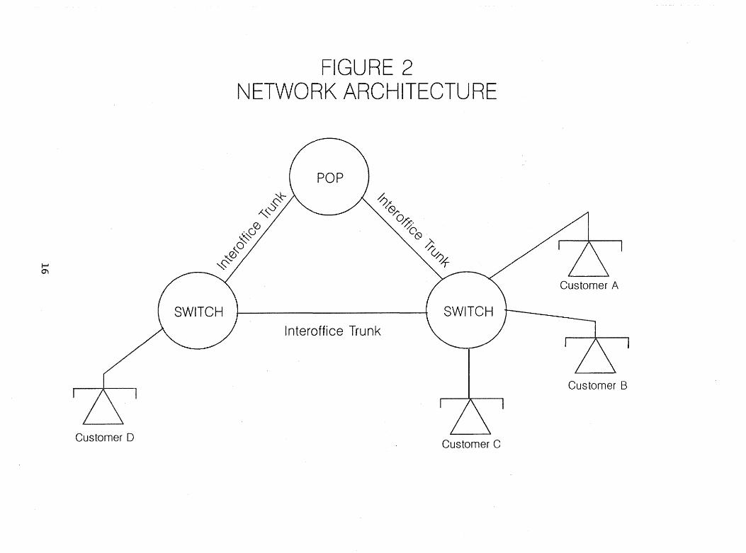
Three primary types of facilities can be found in the local exchange carrier's
network: the local loop, end-office (class five) and tandem switches, and interoffice
transport or trunking. The local loop is composed of facilities that provide a signalling,
voice, video, and data transmission path between a central office and the customer's
station. The central office (or wire center) houses the switching machine that connects a
customer's line either to another customer served by the same switch or to an interoffice
trunk. Calls between central offices are carried on trunks (see figure 2).
15
I-' C"I
Customer 0
FIGURE 2 NETWORK ARCHITECTURE
~ ~.::s
o ~(j
~O ~0
,,-<:'
-0~ (9/:
°0 -/0 (9
Interoffice Trunk
~~ ~1-
Customer C
Local Loop Topology
Telephone engineers break the service territory of a central office into discrete
regions, called serving areas. Since the early 1970s, serving areas have been the basic
building block used to determine the most economical choice of facilities.l A serving
area typically includes 350 to 600 subscribers. Feeder plant connects the service area to
the central office. In turn, distribution ·plant connects the feeder plant to the subscriber,
and is often referred to as the distribution plant.
Figure 3 depicts a typical serving area. A backbone cable runs from the serving
area interface and street cables--or legs--branch off the backbone at equal intervals.
Each time street cables branch off, the backbone cable tapers down.2
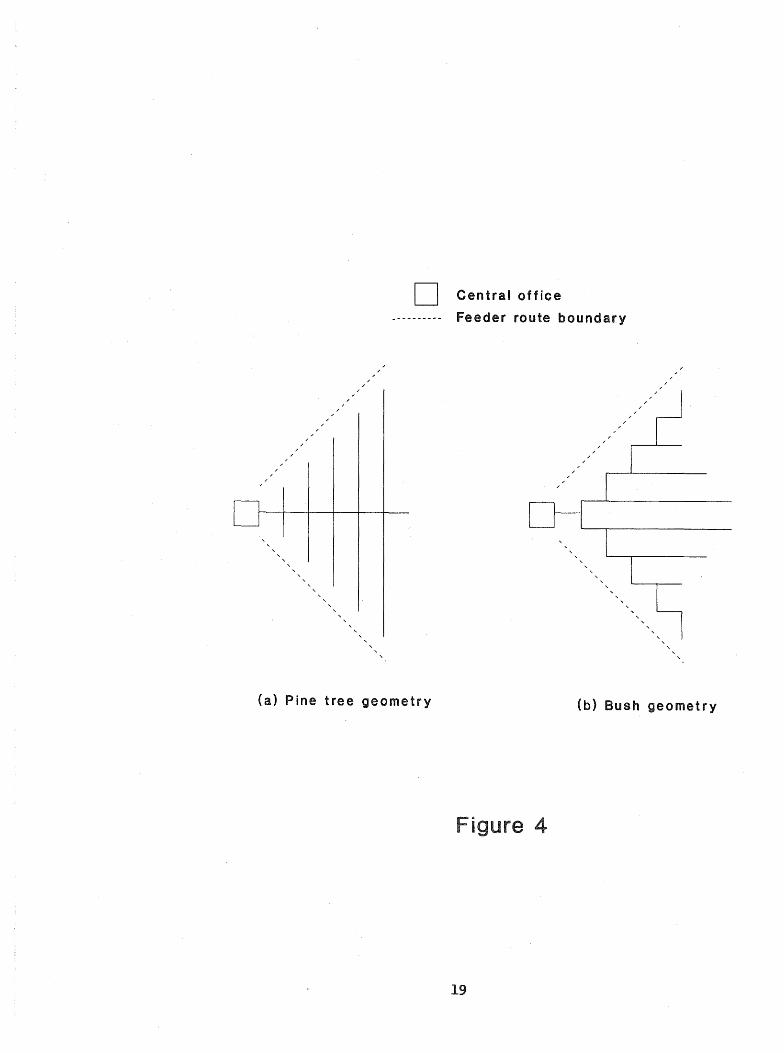
The same design principle is used with feeder plant (Figure 4). Feeder cable runs
from the central office and is connected to a number of branch feeder cables. This
design, known as the "pine tree geometry," minimizes the cost of outside plant facilities.3
lBell Telephone Laboratories, Telecommunications Transmission Engineering: Networks and Services (2nd edition), 40-44; and John Freidenfelds, Capacity Expansion: Analysis of Simple Models with Applications (New York, North Holland, 1981) 238.
The facilities that compose the serving area are commonly referred to as the distribution plant.
2J.A Stiles, "Economic Design of Distribution Cable Networks," Bell System Technical Journal 57 (April 1978): 945.
3Bell Laboratories, Telecommunications Transmission Engineering, 62. The use of the pine-tree topology provides an approximately 5 to 30 percent saving over a bush architecture.
Consistent with engineering practices, we have assumed that the main feeder cables leave the wire center in four directions. Bridger M. Mitchell, "Incremental Costs of Telephone Access and Local Use," Rand R-3909-ICTF (July 1990), 17. The figure depicts one of the four quadrants.
17

INTERFACE
FEEDER NETWORK
(TO CO)
l
DISTRIBUTION TERMINAL ...........................
BACKBONE CABLE
HOUSE /
~ SERVICE WIRE
lEG (STREET) CABLES
igure 3
18
/ /
/ /
D
(a) Pine tree geometry
Central office
Feeder route boundary
(b) Bush geometry
Figure 4
19
The Local Loop: Copper Wires in the Analog Network
Prior to the deployment of digital switches, loop facilities were essentially all
copper wires. Copper cables come in four different sizes: 26, 24, 22 and 19-9auge wire.
The installed size (gauge) of copper wire depends on the distance between the subscriber
and the serving central office. For loops that were located close to the central office,
small diameter, relatively inexpensive copper wire could be used. The drawback to . these
small wires was that they had more resistance than large wires, which could hinder
communications. For this reason, customers more than about 18,000 feet from the
central office were served by larger wire (24, 22 or 19-9auge). Furthermore, on customer
lines more than 15,000 feet from the central office, the resistance design standards
required that load coils be installed to counteract the capacitance of the cables.
During the past ten years, local exchange companies have started to eliminate
load coils from the exchange plant. While these coils served as an effective amplification
device for voice communications, they interfered with high-speed data transmission.4 As
the public switched network is increasingly used for transmitting data at high bit rates,
these coils will be replaced by equipment more suited to digital transmission. Our cost
estimates assume that load coils are still deployed in the local loop.s
4See, for example, Ham Ogiwara and Yasukazu Terada, "Design Philosophy and Hardware Implementation for Digital Subscriber Loops," IEEE Transactions on Communications 30 (September 1982): 2057; and Thomas P. Byrne, Ron Coburn, Henry C. Mazzoni, Gregg W. Aughenbaugh, and Jeffrey L. Duffany, "Positioning the Subscriber Loop Network for Digital Services," IEEE Transactions on Communications 30 (September 1982): 2006-7.
sWhen using LECO M, the user of the model can study the impact of removing the load coils and replacing them with subscriber-Hne-carrier. This is done by changing the crossover point of copper to t-carrier in the program data file DXOVER.DAT to 15 kilo feet (see "Fiber Optics in the Local Loop," 82 infra).
The reader of the report might want to take special note of this and other footnotes were we indicate how the model can be used.
20

Installed Capacity in the Local Loop
The number of cable pairs installed in the feeder and distribution plant is based
on the forecasted number of installed lines. In the 1970s AT&T established a standard
of 1.5 cable pairs per household in the feeder plant, and two pairs per household in the
distribution plant. 6 The number of lines installed for businesses follows similar
engineering rules.
One motivation for allowing two pairs per customer was to have avaHabie capacity
to serve, on demand, customers desiring a second line, which might be needed because
of heavy use by teenagers or for computer communications. Partly out of anticipating
high levels of usage, AT&T decided to provide spare capacity in the feeder and
distribution. We have used these standards for cities where the level of usage falls in the
range of one and 4.2 ccs (ccs= one hundred calling seconds) per main station (see
Table I)? These standards would not be sustained where a customer's usage falls
outside this range.
If usage is "low," less spare capacity would be built into the outside plant facilities.
While busy-hour usage is almost always greater than one ccs, an entrant's deployment of
cable pairs per customer would be a function of usage. If usage is "high," additional
spare would be built into the outside plant because this would raise the probability that
customers would order a second line.
The model can be used to calculate the cost of stand-alone toll systems, whose
usage typically would be below one ccs per customer. By allowing for the different
6J.A. Stiles, "Economic Design of Distribution Cable Networks," Bell System Technical Journal 57 (April 1978): 943.
Post-divestiture, some of the Bell Operating Companies may have adopted different standards.
7The data shown under the column "one to 4.2" are based on standard engineering practices. The data reported in the other two columns were selected by us to reflect how network design changed under different demand scenarios.
21

design criteria, it was our intention to more fully reflect the design principles that would
be followed by an entrant.
Table I Feeder and Distribution Pairs Per Customer
Busy-Hour CCS Usage Per Customer
Less One· to Greater than than one 4.2 4.2
Feeder pairs per 1.10 1.50 1.65 customer (copper)
Feeder pairs per 1.04 1.05 1.08 customer (SLC-96®)
Distribution pairs 1.50 2.00 2.20 per customer
These assumptions imply that within certain ranges of usage the cost of outside
plant facilities will be traffic sensitive in the long run. For example, if usage increased
from .8 to 2.5 busy-hour ccs (bhccs8) per line, the number of distribution pairs per
customer would increase. This, in turn, would raise the cost of the local loop.
For other levels of usage, the number of distribution pairs per customer would be
independent of the level of usage. If usage increased from 2.5 to 3.0 bhccs, there would
be no change in the number of pairs per subscriber.9
~raffic-sensitive equipment is designed to satisfy peak-hour calling requirements. The level of demand is measured at the busiest hour (bh) of the busiest season of the year. Usage is measured in terms of hundred calling seconds (ccs).
~is does not imply that the cost of the loop is nontraffic sensitive. Additional usage may affect the optimal number and location of switches, which, in turn, would make the loop cost traffic sensitive.
22

Placing the Cable Underground
Aerial cable is obviously more exposed to the elements than cables placed
underground. In recent years, to minimize repair problems that may arise from storms,
exchange companies have almost exclusively placed new loop installations
underground.lo
Buried cable is placed in the dirt by a tractor and is installed mostly in suburban
and rural areas where such operations are possible. In urban areas, a utility's right of
way is almost exclusively under paved streets. Consequently, cable must be pulled
through underground conduit. The cost of installing conduit is high--ranging from
approximately $4 to $50 a foot. ll
New Technology in the Local Loop
Digital network topology is significantly different than analog. With analog
switches, the central office served as the exclusive means for concentrating lines into the
switched network. In the digital world, concentration can occur closer to the customer.
As described below, customers may begin sharing facilities at either the serving area
interface or at a remote switching center. When concentration first occurs away from
l°Local exchange companies (LECs) continue to make capital expenditures for aerial cable. These expenditures are typically related to expansion of existing routes or maintenance, rather than the provision of service to new communities.
While our use of LECO M reflects the practice of installing only underground or buried cable, the user of the model can choose to study the cost of using aerial cable by dropping the deployment of underground or buried cable.
llIn our model, we have assumed that only underground and buried cable are used in the local exchange network. The user of LECOM declares in the input file what ratio of buried and underground facilities should be deployed.
23

the central office, the topology is called a double-star architecture, the second star being
the central office.12
We have constructed LECOM under the assumption that in the analog world of
telephony no subscriber carrier is deployed. In the digital version of the model
subscriber line carrier is used where it provides a cost saving. Below we briefly
summarize the engineering procedures for subscriber line carrier.
A. Subscriber Line Carrier
The introduction of digital switching has affected local loop economics. When a
customer is served by a digital switch, voice signals must be converted from an analog to
a digital format at either the central office or at the serving area interface. If the
analog-digital conversion is done in the field, some cost savings can be achieved. Once
the communication signals are converted to a digital format, concentrating a number of
channels on a reduced number of pairs of copper wires or a fiber optic cable becomes
economical.13 The Bell Operating Companies typically deploy SLC-96® (subscriber
line-carrier) for subscriber line concentration.
SLC-96® in an unconcentrated mode14 (Mode-1), the type normally used by the
Bell Operating Companies, provides ninety-six subscriber channels over five copper T-1
digital lines (four working and one protection).15 The T-1lines extend from the central
I2L. Coathup, J.P. Poirier, D. Poirier, and D. Kahn, "Fiber to the Home -Technology and Architecture Drives," 1988 International Symposium Subscriber Lines Services (New York: IEEE, 1988), 14.2.1 - 14.2.5.
13Since we found that subscriber-Hne-carrier on copper was less expensive than subscriber-line-carrier on a fiber optic cable, our discussion here will focus on the former mode of transport.
I4rybe unconcentrated model provides a dedicated voice path to the central office for each customer.
I5Because of one-way transmission, ten copper pairs are used.
24
office terminal to the serving area interface.16 Although rarely deployed by the Bell
Operating Companies, SLC-96® can be configured so that ninety-six voice channels are
concentrated into forty-eight voice paths (Mode-2). By using SLC-96® in a concentrated
mode, only three copper T-1 digital lines (two working and one protection) are needed
to serve ninety-six subscribers.17
With Mode-2 SLC-96®, forty-eight voice channels are available between the
serving area interface and the central office. Because of this two-to-one concentration
ratio, the depioyment of Mode 2 SLC .. 96® raises the likelihood that a subscriber will
receive a busy signal. However, the likelihood is small.I8
In the unconcentrated mode, ninety-six voice channels are provided through ten
pairs of copper wire (Mode 1 SLC-96®). Since each customer is provided with a
dedicated voice channel, use of this configuration does not affect the likelihood that a
customer will receive a busy signal.
The Bell Operating Companies have not widely deployed concentrated SLC-96®
despite significant potential cost savings (an approximate 38 percent first-cost savingsI9),
and a low probability of blockage.2o The Independent Telephone Companies have
I~.A. Abele and A.J. Schepis, "The SLC-96 Subscriber Loop Carrier System: Overview," AT&T Bell Laboratories Technical Journal 63 (December 1984): 2273-2281.
17R.J. Canniff, "A Digital Concentrator for the SLC-96 System," Bell System Technical Journal 60: 121-158.
I8In the concentrated format, SLC-96 mode-2 could carry a load of 12.02 ccs/line and the probability of blockage would be 0.5%. Y -So Cho, J.W. Olson, and D.H. Williamson, "D4 Digital Channel Bank Family: The SLC-96 System," Bell System Technical Journal 61 (November 1982): 2677, 2691. Actual customer usage is approximately one-fourth this level and, consequently, the likelihood of blockage is lower than 0.5%.
19 AT&T System Letter IL 83-06-103, June 13, 1983.
2Dne BOCs reluctance to adopt this cost minimizing technology may be explained, in part, by the poor performance of the concentrators installed in the late 1950s. J.H. Miller and J.G. Schatz, "Loop Concentrators, Present and Future," National Telecommunications Conference: 1977 (New York: IEEE, 1977), 39:1-1 - 1-5. The concentrator technology of thirty years ago was far inferior to the equipment available
25
deployed concentrators more widely in the local loop than the Bell Operating
Companies.21
Wide-scale deployment of SLC-96® by the BOCs was delayed until they began to
install digital switches. When analog switches were the workhorses of the network, SLC·
96® was not economical because the analog-digital conversion had to be done both at the
serving area interface and at the central office. The digital signal could not be processed
by the analog switches, so the customer's signal had to be in an analog format before it
entered the switch.
The Bell Operating Companies increased their commitment to digital switching
technology about 1984. Since digital switches were designed to process digital signals,
the SLC-96® lines could be terminated directly on the switch. This provided significant
savings enticing local exchange companies to increase their use of SLC-96® beginning
about the same year.
A more recent development in the local loop has been the replacement of copper
wires with fiber optic cables. When used in conjunction with t-carrier systems, fiber optic
cables are capable of providing connections to thousands of customers through one
cable.
The LECOM user determines in the input file if either Mode-lor Mode-2
subscriber-line-carrier should be deployed.22 The model determines the distance at
today.
21The Independents have deployed equipment that is engineered with a greater degree of pair-gain, that is a higher ratio of customers to physical lines. See, for example, Raymond D. Hayden, Jr., "General Principles of Feeder - Distribution Cable Engineering," 1987 Rural Electrical Administration Engineering and Management Seminar; and Harold T. Mason, "Application of aNew Subscriber Multiplex With Either Analog or Digital End Offices," National Telecommunications Conference: 1981 (New York: IEEE, 1981).
nnis is done through variable SLC MODE. See page 147 for the format of the input file. If SLC MODE is set to one,-SLC-96 Mode one is deployed. If the value is two, SLC-96 Mode two is deployed.
26
which point it becomes economical to use the subscriber-line-carrier on either copper or
fiber.
B. Remotes
In the digital environment, the local loop cost is also affected by deployment of
remote switches. Remote switches are connected to a large host switch (DMS-10()®) and
can terminate approximately 5,700 lines. The remote either can pass all traffic to the
host switch or handle on a stand-alone basis calls that originate and terminate on the
remote.
We assume that a serving area will be attached to a remote if the loop cost of
connecting a customer to the remote is less than the cost of terminating customers on
the host switch. We allow for up to nine remotes to be attached to each host switch.23
Switch Deployment
During the analog era of telephony, Bell Operating Companies· primarily installed
two types of switching machines: the #2BESS and # 1AESS. The smaller of the two,
#2BESS, had a capacity of 20,000 lines and 38,000 busy-hour calls. The #lAESS switch
could handle 128,000 lines and 240,000 busy-hour calls.24
Despite its large capacity, it was not economical to serve all customers with the
#lAESS machine. It was costly to use long loops to connect suburban neighborhoods
with the machine, which often were located in the center of a city. In such a situation
231n a recent cost study conducted by David Gebhardt, Jr., Illinois Bell assumed that five remotes were attached to host switches in low density regions. Illinois Commerce Commission, 89-0033, ex. 18.24, 27. Apparently, Illinois Bell concluded that remotes were not economical in high-density regions. This is likely due to the short length of the loops in high-density areas. Remotes are only included in our cost-minimizing solution if they lower the total cost of service.
24David Talley, Basic Electronic Switching for Telephone Systems (Rochelle Park, NJ: Hayden Book Co., 1982),228-29.
27
the cost of service may be minimized by substituting switching for loops. The #2BESS
machine was used in less densely populated neighborhoods because the fixed cost was
about one-fourth that of the #lAESS.
Installing an additional switch is economical if the incremental loop savings equal
or exceed the additional trunking and switching costS.25 To illustrate this condition,
assume that the cost of usage is independent of the number of switches. Because of this
assumption, we need only be concerned about the fixed cost of the switch versus the cost
of loops.
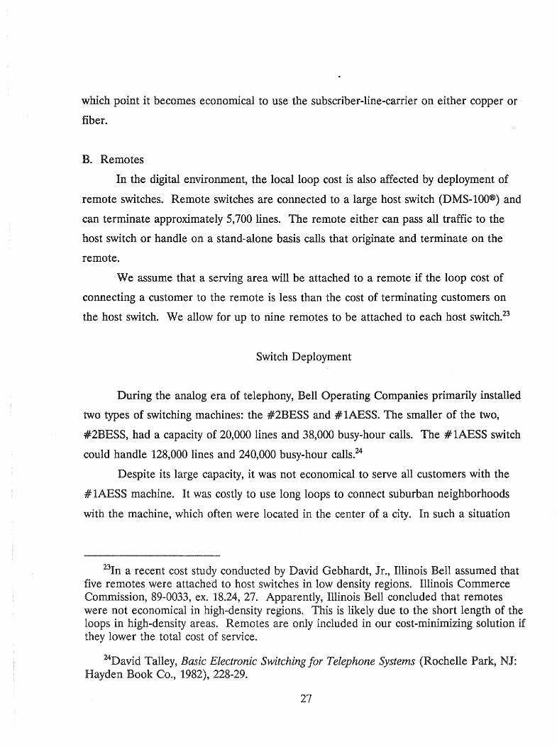
Consider the following diagram.
A B E F G I J K L
Assume that each letter represents an area with a few thousand subscribers served
by two #2BESS switches. The switches are located at points D and H. Alternatively, a
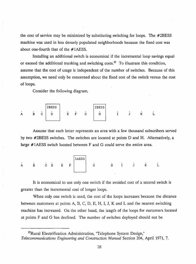
large # 1AESS switch located between F and G could serve the entire area.
A B C D E G H I J K L
It is economical to use only one switch if the avoided cost of a second switch is
greater than the incremental cost of longer loops.
When only one switch is used, the cost of the loops increases because the distance
between customers at points A, B, C, D, E, I, J, K and L and the nearest switching
machine has increased. On the other hand, the length of the loops for customers located
at points F and G has declined. The number of switches deployed should not be
25Rural Electrification Administration, "Telephone System Design," Telecommunications Engineering and Construction Manual Section 204, April 1971, 7.
28
reduced if the incremental cost of longer loops is greater than the switching and trunking
savings that could be achieved by not deploying these switches.
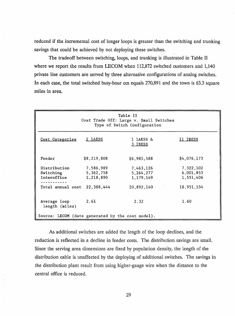
The tradeoff between switching, loops, and trunking is illustrated in Table II
where we report the results from LECOM when 112,872 switched customers and 1,140
private line customers are served by three alternative configurations of analog switches.
In each case, the total switched busy-hour ccs equals 270,891 and the town is 63.3 square
miles in area.
Table II Cost Trade Off: Large v. Small Switches
Type of Switch Configuration
Cost Categories
Feeder
Distribution Switching Interoffice
2 1AESS
$8,219,808
7,586,989 5,362,758 1,218,890
Total annual cost 22,388,444
Average loop 2.61 length (miles)
1 1AESS & 3 2BESS
$6,985,588
7,463,126 5,264,277 1,179,149
20,892,140
2.32
Source: LECOM (date generated by the cost model).
11 2BESS
$4,076,173
7,322,102 6,001,853 1,551,406
18,951,534
1.60
As additional switches are added the length of the loop declines, and the
reduction is reflected in a decline in feeder costs. The distribution savings are small.
Since the serving area dimensions are fixed by population density, the length of the
distribution cable is unaffected by the deploying of additional switches. The savings in
the distribution plant result from using higher-gauge wire when the distance to the
central office is reduced.
29
Switching costs decline because the fixed cost of three 2BESS switches is less than
the fixed cost of the discarded 1AESS machine. The traffic-sensitive costs of the larger
machine are lower, but these savings are smaller than the incremental cost of getting
started.
Interoffice trunking costs increase relative to the option of two 1AESS switches
because the three 2BESS machines terminate fewer lines than the discarded 1AESS
switch. This raises the percentage of intraoffice traffic on the remaining 1AESS .. .,~
machIne.61U
In the digital model, we assume that the supplier deploys either DMS-10Q® or
DMS-IQ® switches. The DMS-IOQ® is capable of processing approximately 300,000 busy
hour busy-season calls. Remote switches, with a capacity of about 5,700 lines, can be
attached to this type of switch. The DMS-1Q® is capable of handling traffic for about
10,000 lines, or 20,000 busy-hour calls.
Toll Office
We have assumed that a city is served by one toll tandem office handling the
traffic going in and out of the city.27 Further, we assume that a #4ESS switch is used
for the toll traffic and that the switch is located in the city's central business district, an
assumption made not only to expedite the search process, but because the location is
consistent with telecommunications engineering practices. If only one switch is used, the
standard engineering rule of thumb is to place the switch in the center of traffic.28
26Intraoffice traffic are calls that originate and terminate on the same switching machine.
27Smaller cities would often be served by a combined toll-local office. Our assumption that each city is served by a toll office does not cause any significant cost distortions since we assume that the cost of toll tandem traffic is linear, with no fixed costs.
28H. Stromberg, "Local Exchange Areas," in International Telecommunication Union Swedish Telecommunications Administration: Planning and Projecting of National Switching
30
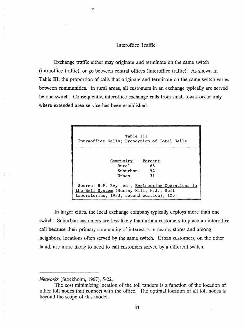
Interoffice Traffic
Exchange traffic either may originate and terminate on the same switch
(intraoffice traffic), or go between central offic,es (interoffice traffic). As shown in
Table III, the proportion of calls that originate and terminate on the same switch varies
between communities. In rural areas, all customers in an exchange typically are served
by one switch. Consequently, interoffice exchange calls from small towns occur only
where extended area service has been established.
Table III Intraoffice Calls: Proportion of Total Calls
Community Percent Rural 66 Suburban 54 Urban 31
Source: R.F. Rey, ed., Engineering Operations in the Bell System (Murray Hill, N.J.: Bell Laboratories, 1983, second edition), 125.
In larger cities, the local exchange company typically deploys more than one
switch. Suburban customers are less likely than urban customers to place an interoffice
call because their primary community of interest is in nearby stores and among
neighbors, locations often served by the same switch. Urban customers, on the other
hand, are more likely to need to call customers served by a different switch.
Networks (Stockholm, 1967), 5-22. The cost minimizing location of the toll tandem is a function of the location of
other toll nodes that connect with the office. The optimal location of all toll nodes is beyond the scope of this model.
31

Traffic studies show that when an interoffice call is placed, there is a greater
likelihood that it will be placed to a customer served by a nearby switch rather than a
distant machine. For example, a subscriber placing an interoffice call from downtown is
more likely to call another downtown customer than a suburban subscriber.
We have constructed LECOM to take into account business customers being
more likely to place interoffice calls that mostly go to nearby switches. The percent of
intraoffice calls is an increasing function of the number of customers terminated on the
customer's host switch divided by the number of switched customers in the city.29
Customer Density
The cost of telephone service is also a function of customer density. An increase
in customer density may lower the average cost of service because as density increases,
the network's fixed cost can be shared by more customers.
29For example, for business customers, we use the following algorithm: percent of exchange calls that are intraoffice calls ::::
0.1735358 + 0.826 *pct where pet :::: x/y
x :::: number of customers on the same switch as the business customer y :::: total number of switched customers in the city For example, assume that pct is equal to 45%. The following percentage of
exchange calls would be intraoffice calls: 0.1735358 + 0.826*.45 :::: .5452. The remaining 45.48% of exchange calls would be interoffice exchange calls.
The formula, 0.1735358 + 0.826*pct was derived by looking at subscriber line usage studies, and observing that as the size of the market increased, the percent of interoffice calls increased (or conversely, the percent of intraoffice calls declined). Larger local markets are typically served by multiple central offices. Based on our reading of the studies, we fitted curves to represent this relationship.
Similar relationships were estimated for the residential and mixed districts, as well as private line customers.
Note that the equation provided in this footnote is the percentage of exchange traffic that is intraoffice. Table III reports the percentage of total traffic that is intraoffice.
32
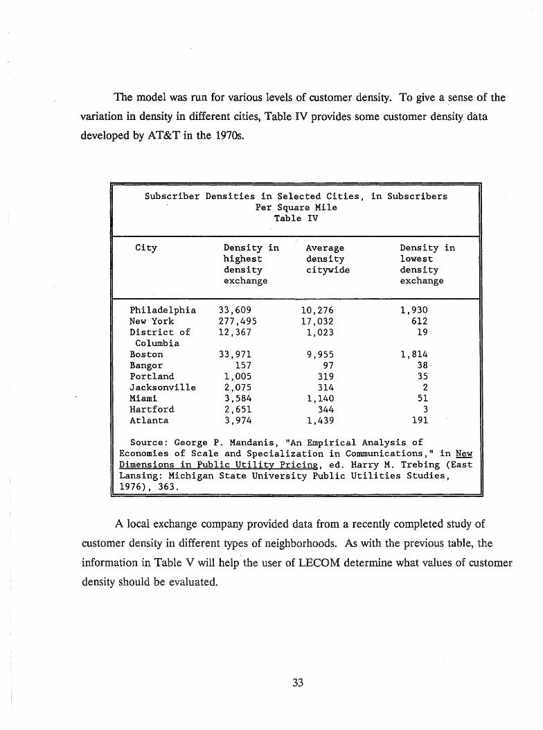
The model was run for various levels of customer density. To give a sense of the
variation in density in different cities, Table IV provides some customer density data
developed by AT&T in the 1970s.
Subscriber Densities in Selected Cities, in Subscribers Per Square Mile
City
Philadelphia New York District of
Columbia Boston Bangor Portland Jacksonville Miami Hartford Atlanta
Table IV
Density in highest density exchange
33,609 277,495 12,367
33,971 157
1,005 2,075 3,584 2,651 3,974
Average density citywide
10,276 17,032 1,023
9,955 97
319 314
1,140 344
1,439
Density in lowest density exchange
1,930 612
19
1,814 38 35
2 51
3 191
Source: George P. Mandanis, "An Empirical Analysis of Economies of Scale and Specialization in Communications," in New Dimensions in Public Utility Pricing, ed. Harry M. Trebing (East Lansing: Michigan State University Public Utilities Studies, 1976), 363.
A local exchange company provided data from a recently completed study of
customer density in different types of neighborhoods. As with the previous table, the
information in Table V will help the user of LECOM determine what values of customer
density should be evaluated.
33

Table V Customer Density per Square Mile
Type of Neighborhood
Single-family High Density Residential
(high rise apartments) Office Park Industrial Park Medium Density Business High Density Business Commercial Strip
(Linear Mile) Source: Proprietary.
Density per Square Mile
2,560 -20,480
7,680 -1,280 -
3,840 49,960
10,240 11,536
5,120 - 7,680 153,600 - 179,200
614
III. Assumptions (A) and Definitions (D) in the Model
In this section we outline some additional assumptions made in constructing
LECOM. As previously discussed, the model is largely based on standard
telecommunication engineering practices. In order to keep the program tractable, some
important assumptions had to be made. They are outlined in this section of the paper.
A (1). The city being selVed by the telephone system can be characterized
geographically by three nested rectangles. This assumption enables a simple space
allocation rule for serving areas, discussed below. It is not in itself unduly restrictive,
since the dimensions of the rectangles are user-declared values (see figure 5).
34

IYT L Y
SUBURBAN
(MOD) MIXED COMMERCIAL/RESIDENTIAL
CENTRAL BUSINESS DISTRICT
(CBO)
Figure 5
35

D(l). The innermost rectangle is known as the central business district (CBD), the
region between the CBD arid the rectangle surrounding it is known as the medium density
district (MDD), and the area outside the MDD but within the city limits is !mown as the
suburbs.
A (2). Within each area population density is uniform. This assumption is
somewhat restrictive, but not wholly unrealistic especially given that we allow differing
densities for the three districts.
D(2). A serving area (SA) is a rectangular geographic area within a district
containing a fixed number of customers. The number of customers in each serving area is
approximately the same throughout the city. A typical serving area includes 600
customers, although this value can be changed by our software users.
A (3). The dimensions of serving areas are determined by the shape of the district
and the percentage of the city's area that lies within that district. Ideally, the dimensions of
serving areas would be computed endogenously as part of the optimization process we
describe later. However, such an optimization would raise the computational burden
considerably and would most likely require the use of a super computer for its solution
(especially in the context of the repeated optimizations we perform here). Instead, we
employ a simple rule: Divide each district into rectangles of equal size such that the
required number of customers per serving area resides in each rectangle.
A (4). There are two types of analog switches, lAESS and 2BESS, and three types of
digital switches, remotes, DMSl ()® and DMSIO()®, each with a unique capacity. In the
digital environment, subscriber line concentrators, also with unique capacities, will be
deployed where they lower the cost of service. This assumption simply reflects the
available technologies. As we will discuss later, part of the optimization problem solved
in this model is a combinatorial optimization over the various feasible mixtures of these
technologies.
36

General Program Description
The programs, which have been written in Pascal (one program is dedicated to
the analog environment, one for the digital) take the annual costs of land, labor,
materials, and capital, as well as the size of the city and customer demand patterns as
inputs. With these input data, the minimum possible number of central offices (given
the capacity of the largest feasible switch) is computed. At this point, the main routine
conducts a search of feasible combinations of central office types for the cost minimizing
arrangement. For each combination of switches, starting locations are estimated by
spacing the switches of each type in intervals between the city boundaries. The program
then searches for other switch locations that will lower the cost of service. For each
location, the cost of an exchange network is computed using the input data, and the
switching, distribution, trunking, and feeder cable algorithms compiled from engineering
studies. The locations of the switches are optimized by a nonlinear, derivative-free,
downhill-simplex routine proposed by NeIder and Mead (1965) and described in Press in
other words.30
»William H. Press, Brian P. Flannery, Saul A. Teukolsky, and William T. Vetterling, Numerical Recipes: The Arl of Scientific Computing, Cambridge, MA (Cambridge University Press, 1986).
The simplex is constructed by augmenting a vector of starting values with a matrix formed by adding the starting value vector to each column of an identity matrix of order equal to the order of the vector in which the diagonal elements have been replaced with appropriate scalars. These scalars are chosen heuristically in the program to be the value halfway between the current cell in the starting value vector and a value on the boundary of the feasible solution set. The algorithm works by taking a series of steps, most of which consist of finding the vertex on the simplex with the highest function value and reflecting it through the opposite face. The same operation is performed on the new simplex, and the process is continually repeated. If a reflection seems to bring about no improvement, the simplex shrinks itself and the algorithm restarts. If the algorithm reaches a point where no further improvements seem possible, it will continue to shrink the simplex until all vertices are within the user-defined tolerance of each other, and convergence is achieved. The user can also specify a maximum number of iterations to allow the algorithm, in which case the routine passes back its best effort for the given number of iterations.
37
Whereas the switch location may be a local rather than a global cost-minimizing
location, we restart the program by randomly adjusting the starting values. The number
of random restarts is determined through the user interface.
The cost computation depends on a crucial simplifying assumption: serving areas
are added sequentially to each switch until a central office's capacity is exhausted.31 A
serving area is attached to the switch located the shortest distance from its serving area
interface. Distance serves as a monotonic approximation of the cost-minimizing solution.
This procedure relieves the potentially massive computational burden of performing a
high-dimensional integer optimization in allocating serving areas to switches.
While it is not computationally feasible to test every possible combination of
serving areas and switches, we allow the model to consider "gains from trading. II After
attaching each serving area to a central office, we look to see if the cost of production
could be reduced by having one switch trade serving areas with another.32 The serving
Press et al. recommend that the algorithm be restarted using any claimed minimum as a new starting vector. The program incorporates this recommendation, allowing the user to specify how many restarts s /he wishes to implement.
3IThe user declares the percent of the switches' theoretical capacity that may actually be used. For the results reported herein, we assume that up to 90 percent of the theoretical capacity is in use.
32Consider the following example. Assume that there are two switches, A and B, and six serving areas. The assumed cost of attaching each of the serving areas to the two switches is shown below:
Serving Area
1 2 3 4 5 6
Cost of Attaching to A 10 12 14 11 35 36
Cost of Attaching to B 15 14 8 7
17 22
In the first pass through the program, the following sequence would occur.
A attaches to serving area 1
38

areas must be exchanged, rather than just changing the assignment of one serving area,
because of the switching machines' capacity constraint. Also, we do not attach a serving
area to a remote switching machine if it would be less expensive to attach it directly to
the host switch. Since the capacity of the host switch is determined in part by the
number of lines attached to the remote, one-way trading may occur.
Once it has been determined which serving areas are served by a switch, "feeder"
routes are determined for the region served by the switch according to the
industry-standard pinetree topology. The pinetree approach minimizes the cost of feeder
plant; the physical plant that distributes telephone signals from the switching office to the
serving area interfaces.
LECOM also takes into account the higher costs of longer loops resulting from
the thicker gauge wire and load coils required to ensure good quality signal transmission.
These computations are stored in a matrix of feeder lengths and gauge distributions.
This matrix is also employed in computing distribution plant costs (within serving areas).
In the digital program, subscriber-line carrier is deployed on the longer loops.
Analog switching costs for the lAESS and 2BESS switches depend on user
declared busy-hour usage by each type of customer class, the presence of other switches
in the local network, and the number of customers served by the switch. Usage patterns
can affect the capacity of switches, especially 2BESS. The program enables
recomputation of 2BESS capacity internally to handle this problem.
The program, then, essentially nests an inner location optimization (that is, finding
the best location of the switches) in an outer combinatorial optimization (that is,
B attaches to serving area 4 A attaches to serving area 2 B attaches to serving area 3 A attaches to serving area 5 B attaches to serving area 6
The program would then search for gains from trade. The cost of the outside plant can be reduced by offices A and B trading serving areas 4 and 5 respectively. The savings associated with attaching serving area 4 to switch A (14 = 35 - 11) exceeds the additional cost of attaching serving area 5 to switch B (10 = 17 -7.).
39
experimenting with different combinations of switches). After the combinatorial search
of switches the program reports the cost minimizing arrangement and location of
switches as well as summarizes relevant input data.
Cost minimization is defined in terms of minimizing the annual production costs,
equivalent to minimizing the present worth of capital, maintenance, and tax
. expenditures.33
Whose Costs Are Being Modeled?
LECOM is designed to determine the network configuration that minimizes the
cost of production. In seeking the optimal combination and location of switches, the
model is not constrained by existing locations. The LECs, by contrast, are not in this
situation--their investment decisions are affected by the current location of facilities. In
this section of the paper we address the extent to which LECOM's cost estimates provide
insight into the process of determining the reasonableness of the rates of the LECs.34
Microeconomic theory emphasizes that pricing decisions should be based on an
analysis of the costs and benefits associated with changes made at the margin.
Economists disagree whether long-run or short-run marginal costs should be used in the
analysis.35
33J. Freidenfelds, "A Simple Model for Studying Feeder Capacity Expansion," Bell System Technical Journal 57 (April 1978): 821.
34LECOM can also be used to determine the cost-of-production when the facility locations are known. By removing the optimization routine from the program, we have also provided the user of the model with a tool that allows the analyst to determine the cost of production for given switch locations. As described at· page 140, if the user indicates the type and location of switches, the model will estimate the cost of service for the indicated network configuration.
35See, for example, Alfred Kahn, The Economics of Regulation, v.1, chs. 3 and 4. The short .. run is that time period during which the facilities of the telephone company are fixed and cannot be varied except at so substantial a cost that it is never profitable. In the long-run, the firm can alter its equipment.
40

It has become the accepted convention in the industry to quantify long-run
marginal costs. When these studies have been conducted, most notably the Bell LRIC
studies, analysts have assumed that the existing location of the central office is that which
minimizes the cost of production.36 Because of these assumptions, only some of the
inputs are variable. Typically, what is assumed to be variable is the type of technology.
Measured cost'i are characterized as long run because the analyst allows for replacing
existing technology with newer types of equipment.
In our study we have assumed that all inputs are variable. By assuming this, our
model is consistent with the economic notion that in the long run no inputs are fixed.37
While this approach is consistent with economic theory, it raises the question: "Whose
costs are being modeled?" The incumbent firm's investment decisions are affected by its
existing investment. The incumbent solves a dynamic problem: it wants to minimize the
present discounted value of its costs of production given the current state of its network,
which involves considering different expansion paths. Strong assumptions must be made
about the cost and capabilities of new technology, price trends for inputs such as labor,
the discount rate, and future demand patterns. Typically, such studies involve projections
made over a fifteen to twenty year period.
Both approaches, minimizing the present discounted value of a supplier's costs
over fifteen years as well as our static analysis, are consistent with the economic notion
of long-run cost analysis. Our approach is more tractable because it requires less
speculation about future cost and demand levels, and the information requirements are
~e assumption is never tested.
37111n strict economic terms, the concept of long-run marginal costs relates to a hypothetical situation in which all inputs are variable, and a supplier confronts the possibility of installing entirely new facilities, in effect from the ground up. And the 'marginal' relates to the incremental cost of a single unit of output." Affidavit of Alfred E. Kahn, In the Matter of Expanded Interconnection with Local Telephone Company Facilities, FCC CC Docket No. 91-141, page 22, note 26, August 5, 1991.
41

less severe.38 The dynamic optimization approach requires that the analyst collect data
on the utilization rates of individual network components, and the relevant forecasted
growth rates for various services.
Our approach provides an estimate of the long-run cost of production, holding
technology constant. Furthermore, the model provides a method for quantifying "the cost
effect of introducing new technologies. Because of the assumption of no sunk or fixed
investments, the model provides an estimate of the production costs that a rival would
incur. An entrantis planning decisions wouid not be affected by existing facUities
because, by definition, it does not currently have a presence in the market. Therefore,
the model provides a competitive benchmark--it suggests the level of production costs
that would be incurred if an entrant were to provide local telecommunication services.
The model of competitive markets is a reference framework used by economists
and regulators to assess the propriety of regulatory economic policy decisions.39 This
paradigm is used because under certain conditions competitive markets provide the most
efficient use of society's scarce resources and maximize welfare.
Furthermore, the Bell Operating Companies and AT&T have previously based
some of their rates for competitive services on their rival's cost structure. For example,
when the Bell System faced rivalry for bulk private-line services, Bell requested
permission to lower its rates. The proposed rates "were based on the cost structure of
AT&Ts competitors, not those of AT&T itself.,,40
38Por example, it is likely that optical switches will be deployed within the next ten years. An analyst who selects the dynamic optimization methodology would need to make assumptions about the cost and capabilities of these switches. But little information is available about this undeveloped technology.
39See, for example, Charles P. Phillips Jr., The Economics of Regulation: Theory and Practice in the Transportation and Public Utilities Industries (Homewood, Illinois: Richard D. Irwin, Inc. 1965), 69.
40Peter Temin, "Cross-Subsidies in the Telephone Network after Divestiture," Journal of Regulatory Economics 2 (December 1990): 353.
42
In the past there has been an asymmetry in the manner in which cost studies have
been done. While great effort has been placed in identifying the cost of providing
competitive services, there have been comparatively few studies of the cost of providing
monopoly services. The rates for monopoly services have typically been set on a residual
basis. First a commission determines the firm's revenue requirement, and second, the
amount of revenue generated by nonbasic services. The remaining revenue requirement
was recovered from basic telephone service.
Since the divestiture of AT&T there has been an increased interest in determining
the cost of different services. We believe that LECOM can be used to indicate the
costs an entrant would incur. These costs can serve as a competitive benchmark to judge
the reasonableness of the rates for monopoly services.41
IV. Cost of the Technologies ,
In this section of the paper we discuss the price of the inputs used to provide
telecommunication services.
The results reported in chapters four and five are based on 1990 input prices.
Where we had available only prices of inputs purchased in earlier years, we adjusted the
input prices by using telephone price indexes. This adjustment process is widely used
due to the cost of collecting and updating input prices.
Cost Structure of the Local Loop
The cost of providing customer access to the network is largely determined by the
cost of the associated outside-plant facilities. The greater the distance between the
central office and a customer's location, the longer the line; if copper wire is used, the
41Tbe use of unobserved but cost based estimates to judge the reasonableness of rates is used in other regulated industries. See, for example, Interstate Commerce Commission, "Coal Rate Guidelines, Nationwide," Ex. parte No. 347 (Sub .. No. 1), decided August 8, 1985, 1 ICC Reports 2d, 520.
43

diameter of the wire may be larger. Therefore, because of both the length of the
connection and the diameter of the wire, the cost of a local loop is distance-sensitive.42
Outside-plant facilities have a flxed and variable cost component. The fixed cost
per foot is associated with the engineering and placement of the wires underground.
This fixed cost is independent of the number of wire pairs inside the cable sheath while
the variable cost is positively correlated.
Table VI provides the fixed and marginal cost per foot for the various gauges of
copper wire used in the loop. We have followed the convention of estimating a linear
cost function from broad-gauge cost data.43 The cost of different size cables was the
dependent variable, and the size of the cables, along with the intercept term, were the
explanatory variables. The estimated coefficient of the intercept measures the per-foot,
fixed-cost of installing a cable.
42The Bell Operating Companies have traditionally taken the position that even though the cost of the loop is dependent on the distance between the customer and the wire center, the marginal cost of serving each customer is independent of distance. AT&T explained this paradox by noting that a wire center is placed at a location where it minimizes the cost-of-service for all customers. AT&T, "Network Service Costs Methods Manual," volume 8, part 3, section 1.1, April 28, 1978. See, also, Testimony of David H. Gebhardt, Jr. on Behalf of Illinois Bell Telephone, Ex. 18.24, p.3, ICC 89 .. 0033.
43See, for example, Rural Electrical Administration, "Design Techniques of Feeder .. Distribution Cable Engineering," Telecommunications Engineering and Construction Manual, section 231, February 1986, p.B .. 41; and New England Telephone, Massachusetts Department of Public Utility, Docket 86-33, work papers, book 1, tab 1, p.20 of attachment 4.
While not shown here, these investments must be loaded for miscellaneous investments, such as conduit and load coils.
44
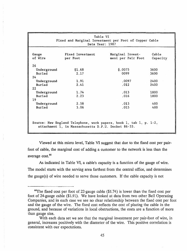
Table VI Fixed and Marginal Investment per Foot of Copper Cable
Data Year: 1987
Gauge Fixed Investment Marginal Invest- Cable of Wire per Foot ment per Pair Foot Capacity
26 Underground $1.68 $.0075 3600 Buried 2.17 0099 3600
24 Underground 1.91 .0097 2400 Buried 2.41 .012 2400
22 Underground 1.74 .013 1800 Buried 2.23 .016 1800
19 Underground 2.58 .013 400 Buried 3.06 .015 400
Source: New England Telephone, work papers, book 1, tab 1, p. 1-2, attachment 1, in Massachusetts D.P.U. Docket 86-33.
Viewed at this micro level, Table VI suggest that due to the fixed cost per pair
foot of cable, the marginal cost of adding a customer to the network is less than the
average cost.44
As indicated in Table VI, a cable's capacity is a function of the gauge of wire.
The model starts with the. serving area farthest from the central office, and determines
the gauge(s) of wire needed to serve those customers. If the cable capacity is not
44tfhe fixed cost per foot of 22 .. gauge cable ($1.74) is lower than the fixed cost per foot of 24 .. gauge cable ($1.91). We have looked at data from two other Bell Operating Companies, and in each case we see no clear relationship between the fixed cost per foot and the gauge of the wire. The fixed cost reflects the cost of placing the cable in the ground, and because of variations in local obstructions, the costs are a function of more than gauge size.
With each data set we see that the marginal investment per pair-foot of wire, in general, increases positively with the diameter of the wire. This positive correlation is consistent with our expectations.
45

exhausted, and if customers located closer to the central office use the same gauge(s) of
wire, the excess capacity is used by the second serving area. When the capacity is
exhausted, an additional cable is installed.
For example, assume that the 600 customers in the serving area the farthest
distance from the central office must be served by 19-9auge wire. Using the standard of
1.5 feeder pairs per customer, the serving area would need 900 pairs of wire requiring
that three cables extend from the central office to the serving area.45 The three cables
have a capacity of 1,200 pairs, but since only 900 pairs are required, 300 pairs are "free"
to be used by a serving area closer to the central office.
Customers are connected to the distribution cable by a drop wire, which goes
from the customer's location to the closest leg in the distribution plant. This investment
varies by the type of customer and the number of customers in the city. The more
densely populated the area, the shorter the drop wire. For a given city, business
customers are generally closer to the distribution leg than residential customers,
reducing the level of investment.
Table VII provides the investment per subscriber drop wire in exchanges of
varying sizes.
For the digital model, we have assumed that SLC-96® equipment may be
deployed on long loops. Esty estimated that the cost of the t-carrier terminal equipment
was approximately $5,000 for twenty-four channels,46 which is in line with data
obtained from other, proprietary sources.
We assume that SLC-96® on fiber, or SLC-96® on copper, is installed where the
annual cost of these technologies is less than providing service via copper cable.
45Round(900/400 + .5). In this example we assume that the full capacity of the cable may be used. But because of the ratio of 1.5 cable pairs per customer, this is an effective fill rate of 66%.
46Scott A. Esty, "Fiber Beats Copper in the Feeder Plant," Telephony, November 16, 1987, 42-46.
46

Table VII 1987 Investment Per Drop Line: Business v. Residential
Primary Calling Area (number of customers)
Less than 15,000 15,000-37,500 37,501-75,000 75,001-120,000 120,001-175,000 175,001-325,000 Greater than 325,000
Business
$42.00 36.60 36.00 23.40 23.40 29.40 6.00
Residential
$81.60 76.80 73.20 70.20 69.60 69.00 31.20
Source: New England Telephone. work papers, book one, tab 1, p. 19, in Massachusetts D.P.U. 86-33.
Fiber Optics
In the digital environment we evaluate the economics of using fiber optics in both
the local loop and in interoffice trunking. The terminal fiber optics costs are a function
of the number of Tl systems. As shown in Table VIII, we allow for a large range of
multiplexers.
Mb/s
45 90 135 405 565
T systems
28 56 84
252 336
Table VIII Fiber Multiplexers
equivalent voice channels 672
1344 2016 6048 8064
investment per end* 8,000
12,000 15,000 22,000 38,500
*Data obtained from Information Gatekeepers, the Rural Electrical Administration, and Esty, flFiber Beats Copper in the Feeder Plant, 42-46. At the rate of 135 MB/s or faster, an additional $10,000 investment per end is needed for each 28 t-carrier systems.
47

We believe that our cost modelling approach provides richer insights than the
methodology often followed by telephone companies. Frequently the telephone
companies calculate transport costs by multiplying unit average costs by the appropriate
quantity. As a result, fixed and variable costs are lumped together. By allowing for
different sizes of multiplexers, we are able to distinguish between large lumpy
investments (for example, the multiplexers), and the smaller incremental costs associated
with increased usage (for example, Tl interface cards and digital cross-connects).
The Cost of Interoffice Calls
The cost of an interoffice trunk is a function of the fixed cost of terminating the
trunk and the distance between the central offices. In the analog mode local exchange
companies essentially choose between two technologies: copper wire and t-carrier on
copper wire. The deployment of t-carrier reduces the number of copper pairs between
offices, but, due to the channel banks, raises the fixed cost of service. For short
distances, copper wire technology minimizes annual costs. For longer distances, t-carrier
is more efficient because the savings in copper wire exceed the higher fixed cost of
terminating the t-carrier.
Our model is designed to determine at what distance the technology of choice
changes from copper wire to t -carrier. F or all interoffice trunks shorter than this
crossover point we calculated the cost of interoffice transport based on copper
technology. For longer distances, trunking costs are based on the assumed deployment
of t-carrier.
In the digital regime the choices are different. Analog copper interoffice trunks
are not cost effective because of the expense of analog-digital conversion. Here we
assume instead that the engineer is choosing between t-carrier on copper wire and too
carrier on fiber optics. T -carrier on copper is the technology of choice for low-volume,
short .. distances routes.
48
Private-Line Costs
Private-line loops are more expensive to provide than ordinary telephone service
because of more stringent technical requirements of data and video services. Prior to
the advent of digital technology in the loop, private-line loops often had to be
engineered individually, an expensive process.47 We have assumed that the cost of a
private-line loop for a given length and customer density is approximately 50 percent
higher than a loop used for IDlalog switched services.48 The data that we have seen
suggests that this difference persists in the digital world. For the digital model, we
assume a mark-up factor of 45 percent.
This additional cost, attributable to the more stringent technical requirements of
private-line services, introduces into our model the possibility of diseconomies of scope.
The cost of the private-line loops is reduced when customers are located close to the
central office. By placing the central office close to the private-line customers (who are
primarily located in the center of a city), the distance may increase between the POTS
47Byrne, et aI., 2006; G.J. Handler and D. Sheinbein, "Improving the Loop to Provide New Network Capabilities," in Proceedings 1982 International Symposium on Subscriber Loops and Services (New York: IEEE, 1982), 1-1; Arvina Karia and Salvatore Rodi, "A Digital Subscriber Carrier System for the Evolving Subscriber Loop Network," The Institute of Electrical and Electronics Engineers, Inc. Transactions on Communications 30 (September 1982), 2013; and Testimony of Leon J. Titman on Behalf of New York Telephone, New York Public Service Commission Proceeding on Telephone Services that Bypass Local Exchange or Toll Networks (28710), December 11, 1984, 2657.
48Based on the data presented in the articles cited in the prior footnote, this factor may be too low. Furthermore, many private line customers are served by two-pairs of cable, rather than the single pair used for plain-old-telephone service. These higher costs are partly offset by the relatively lower cost of providing alarm and burglary service. Balancing these two affects, we arbitrarily assume that private line loops cost about fifty percent more than ordinary loops. In the analog regime, we have assumed that the cost of an interoffice private line trunk is no more expensive than the cost of a POTS trunk. In the digital world, the cost of a private line trunk is greater due to the need to deploy channel banks.
49
(Plain Old Telephone Service) customelS and the closest central office. The additional
distance would cause an increase in the cost of the loop for POTS customers.49
On the other hand, the addition of private-line customers spreads the fixed cost
per foot of cable over a larger number of customers, causing the long-run average cost of
providing POTS access to fall.
Switching Costs
The cost of the analog #2BESS and # lAESS machines (estimated based on
switching-cost-information-system (SCIS) algorithms originally developed by AT&T and
currently supported by Bellcore and SCIS) is used by the Bell Operating Companies to
estimate the cost of switched services.
For the digital switches, we relied on the SCIS algorithms to estimate the level of
remote switching investment. For DMSl()® and DMSIO()®, some information was
obtained from SCIS, while the majority of the algorithms are based on our analysis of
how equipment engineers determine the required facilities.
Input Prices
The cost of production is a function of the available technology, the level of
output, and the price of inputs. The sources for the "baseline" material prices have been
described above.
We have used the model to explore how the cost of production is affected by
changes in the cost of capital, materials, and labor. The annual cost of facilities is
obtained by multiplying the level of investment by plant-specific carrying charges. There
are separate carrying charges for land, buildings, circuit equipment, switching, conduit,
49Diseconomies of scope also may arise when the number of private line customers is held fixed, and the number of switches increases. The additional switches will raise the cost of private-line interoffice trunking.
50
underground copper cable, buried copper cable, underground fiber cable, and buried
fiber cable.
The annual charge factors per dollar of investment are derived from the following
expense categories: maintenance, depreciation, administrative expenses, and taxes. We
define the price of labor as the sum of the maintenance and administrative portions of
the annual charge factors. The price of capital is equal to the sum of the cost of money
and taxes. Finally, we define the price of materials as equaling the rate of depreciation
on the equipment. Reflecting current practices, the rates of depreciation varies by the
type of equipment (for example, approximately 2 percent for conduit, 6 percent for
switching machines). 50
User Inputs
Table IX provides a list of the some of the user inputs that affect the total cost of
service. A complete list of the user inputs is found on page 145.
5~e user of LECO M may modify the level of the annual charge factors by changing the price of labor, material, or capital. For example, if the price of labor is increased by ten percent, the administrative and maintenance portion of each carrying charge is increased by ten percent. If the user wants to evaluate the impact of a five percent decrease in the price of capital, this may be done by changing the input variable PRICECAP from 1.00 to 0.95.
51

Table IX: LECOM User Inputs
Investment costs* Annual charge factors Geographical dimensions of city Area of business district Area of residential district Area of mixed commercial/residential district Number of residential, business and private line customers Busy-hour usage by customer classes Call mix (toll, exchange) Holding time by type of call Switch utilization Ccs per interoffice trunk Private line cost markup Customers per serving area Undergroundjburied cable mix Block width Private lines Switched lines T-carrier utilization rate Loop utilization rate
*Most of our investment cost data came from Bell Operating Companies, the Rural Electrical Administration, and public sources. The only major departure that we make from conventional data sources is our assumption regarding analog switch pricing trends since 1984. Prior to divestiture, AT&T was the sole supplier of analog switches to the Bell Operating Companies. As part of its incentive to get BOCs to migrate to digital switches, AT&T has priced analog switches at prices that depart radically from price trends with similar (PBXs) and like products (for example 8088 microcomputers). The pricing pattern has also departed from the life-cycle pricing history of competitive electronic products (for example VCRs). We assume that after 1984, that the price of analog switches increases (decreases) at the same rate as digital switches.
We evaluated the impact of substituting our telephone plant index for analog switching, for the higher index used by the telephone companies (the telephone company index for analog electronic switching machines was approximately 89% higher).
We found that this change raised the total cost of service on an analog network by six to seventeen percent. The seventeen percent increase occurred in smaller cities, where under both scenarios, LECOM said that it was optimal to deploy only one switch.
The lower range, six percent, was observed where there were a large number of customers, and LECOM said that multiple switches should be deployed. When the cost of switching increased by 89%, LECOM said that fewer switches should be deployed, and this in turn, increased the length of the local loop.
52
CHAPTER THREE
METHODOLOGY FOR GENERATING DATA
Optimization
In the previous chapter we outlined some of the primary engineering steps that
are used to design a telecommunications network. An important step in constructing
LECOM was ·to reduce these procedures into mathematical relationships. Tnis reduction
is the essence of an engineering process model--expressing engineering functions in a
series of equations.
For example, when operating at full capacity, a t-carrier system is designed to
simultaneously carry twenty-four voice conversations. The number of t-carrier systems
required between two points is determined by dividing the number of voice channels by
twenty-four, and rounding up to the next integer. The following equation illustrates this
process:
t-carrier = round(x/24 + .5),
where x = the number of voice channels.
If twenty-six voice channels needed to be installed between points a and b, the
equation tells us that two t-carrier systems should be deployed [2 = t-carrier = round(26/24 + .5).
Mter determining the facility requirements, LECOM multiplies the applicable
physical quantities by their respective prices. If one end of a t-carrier system costs
$5,000, the model would report that the cost of terminating the two t-carrier systems as
being $10,000 ($5,000 x 2 t-carrier systems).
We have undertaken similar process representations for all components of the
network (that is, the local loop, switching and other components of interoffice trunking).
Using these cost algorithms, LECOM searches out for the combination of
facilities that minimizes the cost of production. This is achieved by evaluating both
different combinations of large and small switches, as well as different node locations.
53

Because of the search for the cost minimization location of switches, we are able to
characterize LECOM as an optimization model.
Generating Data
After we completed the construction of LECOM we ran the model a few hundred
times in order to evaluate how changes in the level of demand, as well as input prices,
affected the cost of service. It is through these repeated simulations of our cost modei
that we obtained the data discussed in chapters four and five, and appendix one.
The data generated by the model reflects the current costs incurred by telephone
companies in providing telecommunication services. The input price data used to
generate our results are based on actual cost data (for example, cost per pair-foot of
cable; the cost of a remote switching machine). But unlike telephone cost models, our
estimated cost of service is based on an assumption of optimization behavior; that is,
minimizing the long-run cost of production.
In generating the data, we have tried to take into consideration the need to
evaluate changes in output over a wide-range of outputs (summary statistics are provided
on page 107), as well as an in-depth view of how the marginal cost of production of
service A is affected by an increase in the output of service B. This second objective was
achieved by starting with varying "base cases," and then looking at different, but not all,
increments of the studied services. Table X provides a summary of the different
increments studied for each base case. The list reported in Table X provides twenty-six
observations for regression analysis (the base case and twenty-five increments to the base
case). These same observations can be used to directly calculate the marginal cost of
service (see "Using the Model to Calculate the Marginal Cost of Service, page 106).
54

Table X Combinations Ran in Generating Data
Base case
Incrementing the demand of one service 1 2 345 Incrementing the demand for two services 1,2 3,4 3,5 1,3 1,4 1,5 4,5 Incrementing the demand for three services 5,2,3 5,1,4 5,1,3 5,1,2 5,2,4 Incrementing the demand for four services 5,1,3,4 5,2,3,4 5,1,2,3 5,1,2,4 Incrementing the demand for five services 1,2,3,4,5
Definitions: 1 = Exchange switched service 2 = Toll switched service 3 - Local private line service 4 - Toll private line service. 5 - Switched access
2,3 2,4 2,5
Because of the orthogonal nature of the twenty-six observations referenced in
Table X, the validity of the data is easily evaluated. The twenty-six observations permit
the calculation of the marginal cost of each of the five services in many different ways.l
Sometimes the model will select switch locations that do not minimize the cost of
production. When this occurs, the calculated incremental costs are likely to appear to be
unreasonably low or large. These out-of-range values were corrected using the
methodology described at page 140.
lThe formulas are provided on LOTUS spreadsheets VRESLARG.WK1 and DRESLARG.WKl. The spreadsheets are found on the enclosed disk.
55

CHAPTER FOUR
COST ESTIMATES
In this and the following chapter we provide an analysis of the data generated by
LECOM. As mentioned in the last chapter, we ran LECOM a few hundred times in
order to generate a data base that could be used to analyze the cost structure of the
industry. The more technical results are reported in appendix one. Here we briefly
summarize the econometric resuits rrom the model, provide estirnates of the luarginal
cost of different services, and discuss the extent to which the data indicate that the
industry is a natural monopoly.
In chapter five we use the output from LECOM to analyze the economics of fiber
optics in the local exchange plant and the pricing implications of our study.
Discussion of Econometric Results
Traditionally, the telephone industry has been considered an increasing-cost
industry. 1 The marginal cost of serving a subscriber was believed to be an increasing
function of usage because as the nUPlber of customers on the local network increased,
the number of theoretical connections increased exponentially. In order to be able to
make all of these theoretical possible connections, the switching equipment became
increasingly sophisticated and expensive.2
ISee, for example, John Lee, The Economics of Telegraphs and Telephones (London: Sir Isaac Pitman and Sons, 1913), 74.
2Microeconomic theory suggests that where an industry is characterized by increasing average costs, production costs will be minimized if the product is produced by many small firms. If all firms have a small share or the industry output, they will be operating with a lower average cost than if one firm produced the total output.
Because of customers' desire for universal service, this market structure is not practical for switch telecommunication services. Customers want universal access to all subscribers. Since the various suppliers of switched telecommunication services must interconnect, the atomistic market structure would not provide any cost savings. Because
57
In the early 1980s the view of the industry as being characterized by increasing
average costs was challenged by the econometric work of Christensen et al. 3 who
concluded there were strong economies-of-scale in the Bell System. We have used
LECOM, and traditional statistical tools to further study this issue (see appendix one,
page 93).
The results reported in table B-1, page 96, are in line with the earlier perception
of diseconomies of scale. The estimated coefficient of the squared value of the outputs
is positive. This suggests that the marginal cost of service is an increasing function of
usage.
For exchange service, the increasing marginal cost is likely the result of the
capacity constraint of a switch. Because a given switch can only process a limited
number of calls, at some point additional switches need to be added. Since an
interoffice call is more expensive than an intraoffice call, the cost of an exchange ccs
should increase as the volume of traffic increases.
When only one switch is deployed in a city, it is likely to be located in the center
of town near the toll tandem office. When additional switches are deployed, some will
be located away from the center of town. Because of the additional transport cost, toll
ccs should be an increasing function of usage.4
It is less obvious why the second-order term for access lines should be positive. A
switch can terminate only a limited number of access lines. When that capacity is
exceeded, an additional switch must be added. The deployment of a second switch
of the cost penalty of interoffice trunking, as well as the substantial fixed cost of a switching machine, costs may still be minimized through one supplier, even though that one firm incurs increasing average costs. See, David Gabel, "Deregulation: Should the Local Telephone Market Be Next?" New England Law Review, 24 (1989): 39-61; and the discussion infra at page 69.
3L. Christensen, D. Cummings, and P. Schoech, "Econometric Estimation of Scale Economies in Telecommunications," Social System Research Institute, Discussion Paper No. 8013, University of Wisconsin.
~e cost of toll ccs is also a function of the switch capacity constraint discussed in the prior paragraph.
58
lowers the length of a loop, and this should lead to a reduction in the marginal cost of a
loop. Conceivably, the second-order term for access lines is positive because it is picking
up the quasi fixed cost of deploying additional switches.
It is perhaps because of the lumpy nature of interoffice trunks, as well as the
outside plant cables used in the local loop, that the second-order terms for local and toll
private lines are positive. When the capacity of a cable or an interoffice channel bank is
exceeded, additional, quasifixed costs must be incurred. These costs may be the force
that is causing the second-order terms to be positive.
The cross-product terms indicate that increased usage of one product has a
"' statistically significant effect on the marginal cost of other services. The cost tools used
by the local exchange carriers are not designed to capture these effects and therefore do
not capture the total cost impact of increased usage.
Two product interaction terms are of special interest because of the recent debate
regarding optimal recovery of access line costs. In the analog model, the interaction
term between access lines and toll ccs is not statistically significant. This suggests that
the cost of an access line is independent of toll usage. In the digital model when
homogeneity is imposed,5 the coefficient may be considered statistically significant,
depending on the chosen level of significance and the alternative hypothesis. On the
other hand, the cross term between access lines and exchange ccs is statistically
significant in the analog and digital model. This suggests that exchange usage has a
statistically significant affect on the cost of customer access.
Directly Estimating the Incremental Cost of Service
In studying the cost function, we have analyzed the impact of increasing the
demand for one service while holding all other variables constant. In doing so, we have
constructed what are known as orthogonal data, which allows us to calculate the average
incremental cost of a service without doing any regression analysis (the incremental cost
5See discussion, page 94.
59
is divided by the incremental usage of the one service whose demand has not been held
constant).
We have used this approach to estimate the marginal cost of private line and
switched services, as well as access. The results based on 1990 input prices, from
LECOM, are reported on pages 61 through 67. For each cell the datum is the average
of eleven estimates of the incremental cost of service. The standard deviation for each
estimate is reported in parenthesis.
The data on page 61, Table XI indicates that for a city covering 31.69 square
miles, if a telephone company was to serve 70,508 customers with digital technology, the
total annual cost would be $12,426,213. The same city could be served with analog
technology for $11,398,767. Despite the higher total cost, the marginal cost of switched
exchange and toll ccs is lower with digital technology. The costs are $6.72 and $14.29
respectively per bhccs, versus $8.29 and $29.64 with analog technology. The cost of local
private line service is also lower, $135.26 versus $157.76 on the analog network. On the
other hand, the annual marginal cost of private line services and switched access are
higher on the digital network. The annual cost of switched 'access is $87.81 on the digital
network, and $71.84 with analog technology. While the annual marginal cost of toll
private line service would be $243.92 with analog technology, on a digital network it
would be $340.69.
60
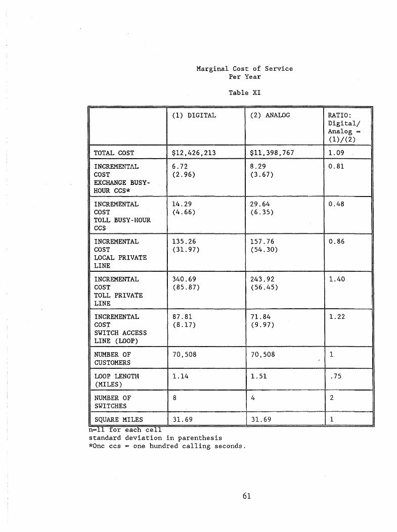
TOTAL COST
INCREMENTAL COST EXCHANGE BUSY-HOUR CCS*
INCREMENTAL COST TOLL BUSY-HOUR CCS
INCREMENTAL COST LOCAL PRIVATE LINE
INCREMENTAL COST TOLL PRIVATE LINE
INCREMENTAL COST SWITCH ACCESS LINE (LOOP)
NUMBER OF CUSTOMERS
LOOP LENGTH (MILES)
NUMBER OF SWITCHES
SQUARE MILES n .... ll tor each cell
Marginal Cost of Service Per Year
Table XI
(1) DIGITAL (2) ANALOG
$12,426,213 $11,398,767
6.72 8.29 (2.96) (3.67)
14.29 29.64 (4.66) (6.35)
135.26 157.76 (31.97) (54.30)
340.69 243.92 (85.87) (56.45)
87.81 71.84 (8.17) (9.97)
70,508 70,508
1.14 1.51
8 4
31.69 31.69
standard deviation in parenthesis *Onc ccs - one hundred calling seconds.
61
RATIO: Digital/ Analog .... (1)/(2)
1.09
0,81
0.48
0.86
1.40
1.22
1 ,
.75
2
1

Table XII
DIGITAL ANALOG RATIO
TOTAL COST 9,472,592 8,315,164 1.14
INCREMENTAL $1.53 3.57 .43 COST (0.69) (1.24) EXCHANGE BUSY-HOUR CCS
INCREMENTAL 13.28 22.85 .58 COST (0.64) . (5.75) TOLL BUSY"HOUR CCS
INCREMENTAL 137.22 116.07 1.18 COST (28.90) (33.21) LOCAL PRIVATE LINE
INCREMENTAL 402.60 163.09 2.47 COST (145.12) (77.29) TOLL PRIVATE LINE
INCREMENTAL 136 99.75 1.36 COST (1.79) (3.12) SWITCH ACCESS LINE (LOOP)
NUMBER OF 56,420 56,420 1 CUSTOMERS
LOOP LENGTH 1.034 1.74 .59 (MILES)
NUMBER OF 6 1 6 SWITCHES
SQUARE MILES 23.08 23.08 1
62
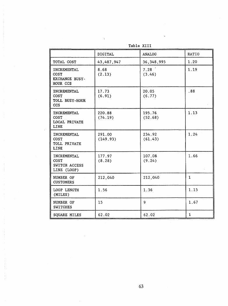
Table XIII
DIGITAL ANALOG RATIO
TOTAL COST 43,487,947 36,348,995 1.20
INCREMENTAL 8.68 7.28' 1.19 COST (2.13) (3.46) EXCHANGE BUSY-HOUR CCS
INCREMENTAL 17.73 20.05 .88 COST (6.91) ({:. 77\ \.., • , , I
TOLL BUSY-HOUR CCS
INCREMENTAL 220.88 195.76 1.13 COST (74.19) (52.68) LOCAL PRIVATE LINE
INCREMENTAL 291.00 234.92 1.24 COST (149.93) (61.43) TOLL PRIVATE LINE
INCREMENTAL 177.97 107.08 1.66 COST (8.28) (9.24) SWITCH ACCESS LINE (LOOP)
NUMBER OF 212,040 212,040 1 CUSTOMERS
LOOP LENGTH 1.56 1.36 1.15 (MILES)
NUMBER OF 15 9 1.67 SWITCHES
SQUARE MILES 62.02 62.02 1
63

Table XIV
DIGITAL ANALOG RATIO
TOTAL COST 25,549,965 20,200,009 1.26
INCREMENTAL $3.53 11.25 .31 COST (1.00) (2.78) EXCHANGE BUSY-HOUR CCS
INCREMENTAL 20.21 28.59 .71 COST (7.74) (8.96) TOLL BUSY-HOUR CCS
INCREMENTAL 151.51 129.74 1.17 COST (23.63) (29.89) LOCAL PRIVATE LINE
INCREMENTAL 360.86 193.67 1.86 COST (86.04) (63.57) TOLL PRIVATE LINE
INCREMENTAL 112.69 51.12 2.20 COST (2.78) (2.18) SWITCH ACCESS LINE (LOOP)
NUMBER OF 179,000 179,000 1.0 CUSTOMERS
LOOP LENGTH 0.89 0.78 1.14 (MILES)
NUMBER OF 4 4 1.0 SWITCHES
SQUARE MILES 8.12 8.12 1.0
64
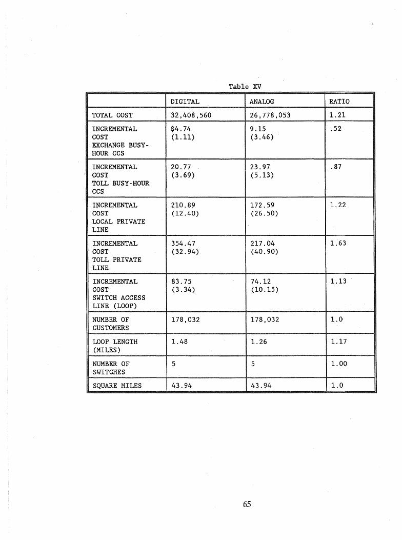
Table XV
DIGITAL ANALOG RATIO
TOTAL COST 32,408,560 26,778,053 1.21
INCREMENTAL $4.74 9.15 .52 COST (1.11) (3.46) EXCHANGE BUSY-HOUR CCS
INCREMENTAL 20.77 23.97 .87 COST (3.69) (5.13) TOLL BUSY-HOUR CCS
INCREMENTAL 210.89 172.59 1.22 COST (12.40) (26.50) LOCAL PRIVATE LINE
INCREMENTAL 354.47 217.04 1.63 COST (32.94) (40.90) TOLL PRIVATE LINE
"
INCREMENTAL 83.75 74.12 1.13 COST (3.34) (10.15) SWITCH ACCESS LINE (LOOP)
NUMBER OF 178,032 178,032 1.0 CUSTOMERS
LOOP LENGTH 1.48 1.26 1.17 (MILES)
NUMBER OF 5 5 1.00 SWITCHES
SQUARE MILES 43.94 43.94 1.0
65
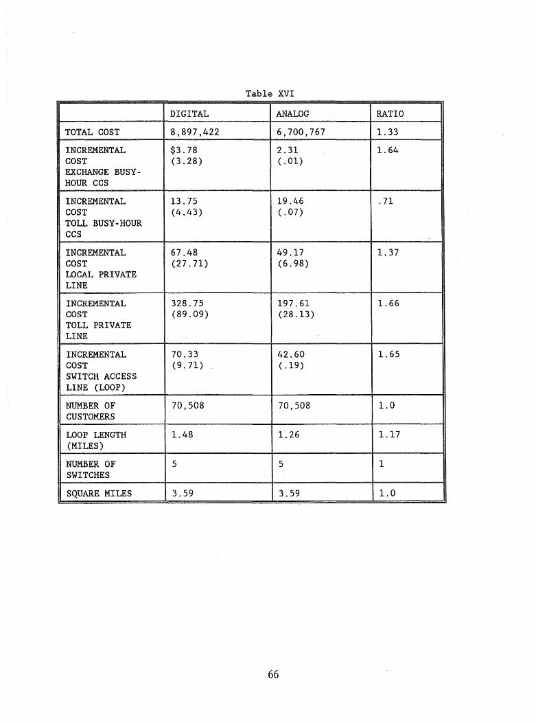
Table XVI
DIGITAL ANALOG RATIO
TOTAL COST 8,897,422 6,700,767 1.33
INCREMENTAL $3.78 2.31 1.64 COST (3.28) (.01) EXCHANGE BUSY-HOUR CCS
INCREMENTAL 13.75 19.46 .71 COST (4.43) (.07) TOLL BUSY-HOUR CCS
INCREMENTAL 67.48 49.17 1.37 COST (27.71) (6.98) LOCAL PRIVATE LINE
INCREMENTAL 328.75 197.61 1.66 COST (89.09) (28.13) TOLL PRIVATE LINE
INCREMENTAL 70.33 42.60 1.65 COST (9.71) (.19) SWITCH ACCESS LINE (LOOP)
NUMBER OF 70,508 70,508 1.0 CUSTOMERS
LOOP LENGTH 1.48 1.26 1.17 (MILES)
NUMBER OF 5 5 1 SWITCHES
SQUARE MILES 3.59 3.59 1.0
66
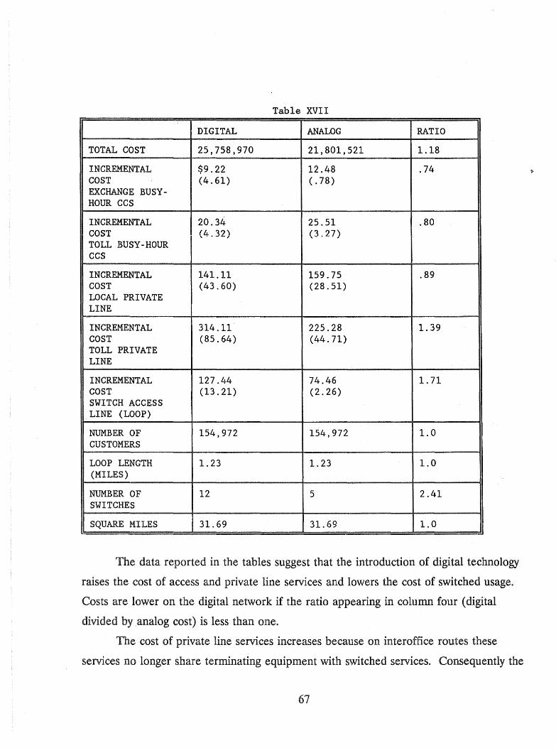
Table XVII
DIGITAL ANALOG RATIO
TOTAL COST 25,758,970 21,801,521 1.18
INCREMENTAL $9.22 12.48 .74 COST (4.61) (.78) EXCHANGE BUSY-HOUR CCS
INCREMENTAL 20.34 25.51 .80 COST (4.32) (3;27) TOLL BUSY-HOUR CCS
INCREMENTAL 141.11 159.75 .89 COST (43.60) (28.51) LOCAL PRIVATE LINE
INCREMENTAL 314.11 225.28 1.39 COST (85.64) (44.71) TOLL PRIVATE LINE
INCREMENTAL 127.44 74.46 1.71 COST (13.21) (2.26) SWITCH ACCESS LINE (LOOP)
NUMBER OF 154,972 154,972 1.0 CUSTOMERS
LOOP LENGTH 1.23 1.23 1.0 (MILES)
NUMBER OF 12 5 2.41 SWITCHES
SQUARE MILES 31.69 31.69 1.0
The data reported in the tables suggest that the introduction of digital technology
raises the cost of access and private line services and lowers the cost of switched usage.
Costs are lower on the digital network if the ratio appearing in column four (digital
divided by analog cost) is less than one.
The cost of private line services increases because on interoffice routes these
services no longer share terminating equipment with switched services. Consequently the
67

lumpy investments are no longer shared by as many customers. Furthermore, in today's
digital environment carriers are only installing digital interoffice trunks, even though
analog copper trunks may be the cost-minimizing technology for many private line
interoffice trunks.
The cost of terminating an access line increases because the line termination
equipment on a digital switching machine handles many functions that were previously
the function of interoffice trunking equipment and the central processor unit of the
switching machine.6 Because the access line termination equipment handles these
functions, ccs related costs decline.
Why Might the Loop Length Increase When the Number of Switches Deployed Increases?
The data in table XIII shows that in the digital environment cost is minimized by
deploying fifteen switches, six more switches than in the analog environment. Despite
the larger number, the loop length is longer (1.56 miles for digital, 1.36 for analog). This
anomaly is the result of the unique capacity of the switches. As we reported earlier the
analog 2BESS switch has a capacity of 20,000 lines. The DMS1()® switch has a capacity
of 10,000 lines, and a remote switch attached to a host can terminate 5,720 lines. Of the
fifteen switches referenced in table XIII, seven were remotes and seven were DMS1()®
switches. These fourteen switches have a theoretical capacity of 109,000 lines. Those
6A multiproduct firm, such as a telephone company, is often able to provide a number of services at a lower cost than if each product was produced by different companies. A major source of these economies of scope is cost complementarities, that is, "that the marginal cost of producing anyone product decreases ... with increases in the quantities of other products." Baumol, Panzar, and Willig, Contestable Markets, 74-75.
"Access service" does not exhibit this property. The marketing of digital services on the same network used for exchange voice service raises the marginal cost of access. . If there were a product such as access service, there would be an economic incentive for access to be provided on 'a stand-alone basis unless none of the additional cost of access was included in the price of access.
68

customers not attached to one of these switches are attached to the host switch (a
DMS10()®).
In the analog environment, eight of the nine switches were 2BESS machines with
a combined theoretical capacity of 160,000 lines. Those customers not attached to one
of these 2BESS machines must be attached to the 1AESS switch.
Since the eight 2BESS machines have more capacity than the seven remotes and
seven DMS1()® machines, the loop length is longer in the digital environment. Those
custoIIH~rs not attached to a nearby switch win be attached to the large s\vitch (either the
DMS10()® or 1AESS). To reach the large switch, the average length of connection is
longer in the digital environment.
Is the Local Exchange Market a Natural Monopoly?
An industry is considered a natural monopoly if and only if a single firm can
produce the desired output at lower cost than any combination of two or more firms.
This property, known as sub additivity of the cost function, holds if for any set of goods N
= 1, ... n, and for any m output vectors Ol ... OM of the goods in N7:
C(Ol) + C(02) + ... C(OM) > C(Ql +Q2 ••• OM)·
This equation merely states it is cheaper for one firm to produce all output than
two or more firms.
This condition has little to do with the popular notion of a natural monopoly,
declining average costs. For a multiproduct industry, scale economies are neither
necessary nor sufficient for a natural monopoly.8
7William J. Baumol, "On the Proper Cost Tests for Natural Monopoly in a Multiproduct Industry," American Economic Review 67 (December 1977): 810.
8Ibid., 817. Neither is it necessary for a single product industry. Consider the following cost function.
if q ~ 8, c( q) = 6 + 2q if q > 8, c( q) = 10 + 2q
69
A necessary, but not sufficient condition for a natural monopoly is economies of
scope. This property is illustrated by the following equation:
C(01'O) + C( 0,02) > C(01,02)
where 0 1 = the output of product one
O2 = the output of product two.
The equation merely states it is cheaper to have product one and two produced by
a single firm [C(Q1,Q2)]' than by having separate firms produce product one and two
In this section of the paper we provide some data regarding the extent to which
economies of scope are present in the telecommunications industry. A finding that
economies of scope are not present indicates that the industry is not a natural monopoly.
If economies of scope are present, the industry may be a natural monopoly.10
where q = the level of output. When the level of output exceeds 8, the initial capacity is exhausted, and plant
must be expanded. The additional capacity causes the quasi-fixed cost of production to increase by four dollars (10 - 6).
When the level of output is eight, the average cost is 2.75 [c(8)j8 = (6+2*8)/8 = 2.75]. If output increases to nine units, the average cost is 3.11 [c(9)/9 = (10+2*9)/9 = 3.11]. Despite this increasing average cost, it is cheaper for one firm to produce 9 units [c(9) = 28], then to have two firms produce the same output [28 < c(l) + c(8) = 8 + 22 = 30]
9Necessary and sufficient conditions for a natural monopoly are economies of scope and declining average incremental costs. David S. Evans and James J. Heckman, "A Test for Subadditivity of the Cost Function with an Application to the Bell System," American Economic Review 74 (September 1984): 615-16. The results from the translog equation (page 94) suggest that this condition is not satisfied (due to the increasing marginal costs).
Other sufficient conditions for a natural monopoly are discussed by William Sharkey, The Theory of Natural Monopoly (New York: Cambridge University Press, 1982), 67-73.
l~n this paper we do not test to see if the sufficient conditions for natural monopoly are satisfied. As discussed below, the necessary condition is not always satisfied, and therefore we did no! test the sufficiency condition.
70

The results from our optimization model suggest that the local exchange
telecommunications market is not a natural monopoly under all feasible situations. As
illustrated on pages 72 and 74, the cost function does not exhibit economies of scope.
Production costs would be minimized if more than one firm produced local exchange
services.
We have assumed that the firm produces four outputs:ll switched toll and
exchange services, and toll and exchange private line services. Let
X(l) = exchange switched service
X(2) = toll switched service
X(3) = local private line service
X( 4) = toll private line service.
We have estimated the cost of producing these services in common (that is, are all
four services provided through one network), as well as on a stand-alone basis. For
example, we used LECOM to estimate the cost of serving a city with 179,000 customers
spread over 8.12 square miles. We report the results in Table XVIII and Table XIX.
llWhenever toll or exchange switched service is provided, the customer is connected to the switch via an access line. While this cost is included in the tables below, we do not list it as a product because we do not believe that access is a service that would be provided on a stand-alone basis.
71
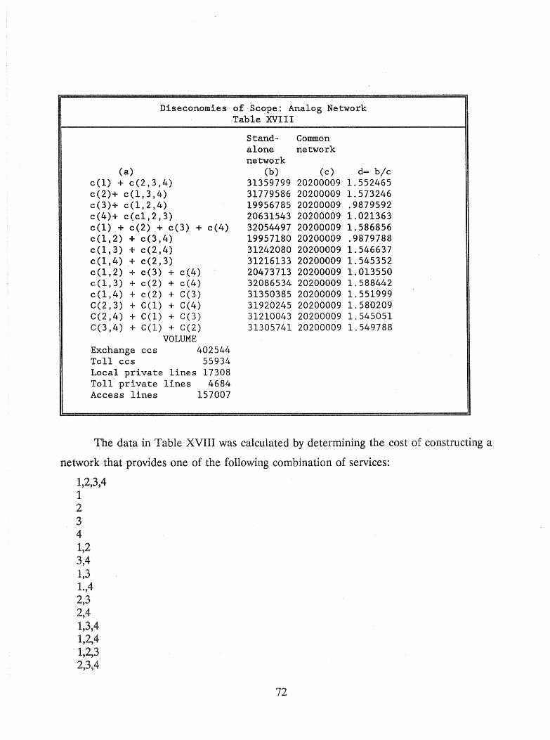
Diseconomies of Scope: Analog Network Table XVIII
(a) c(l) + c(2,3,4) c(2)+ c(1,3,4) c(3)+ c(1,2,4) c(4)+ c(c1,2,3) c(l) + c(2) + c(3) + c(4) c(1,2) + c(3,4) c(l,3) + c(2,4) c(l,4) + c(2,3) c(1,2) + c(3) + c(4) e(1,3) + e(2) + c(4) c(1,4) + c(2) + C(3) C(2,3) + C(l) + C(4) C(2,4) + G(l) + C(3) C(3,4) + G(l) + C(2)
VOLUME Exchange ces 402544 Toll ccs 55934 Local private lines 17308 Toll' private lines 4684 Access lines 157007
Stand- Common alone network network
(b) (e) 31359799 20200009 31779586 20200009 19956785 20200009 20631543 20200009 32054497 20200009 19957180 20200009 31242080 20200009 31216133 20200009 20473713 20200009 32086534 20200009 31350385 20200009 31920245 20200009 31210043 20200009 31305741 20200009
d= b/e 1.552465 1.573246 .9879592 1.021363 1.586856 .9879788 1.546637 1.545352 1.013550 1.588442 1.551999 1.580209 1.545051 1.549788
The data in Table XVIII was calculated by determining the cost of constructing a
network that provides one of the following combination of services:
1,2,3,4 1 2 3 4 1,2 3,4 1,3 1.,4 2,3 2,4 1,3,4 1,2,4 1,2,3 2,3,4
72
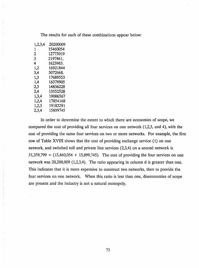
The results for each of these combinations appear below:
1,2,3,4 20200009 1 15460054 2 12773019 3 2197461. 4 1623963. 1,2 16921844 3,4 307266.8. 1,3 17689553 1,4 16379905 2,3 14836228 2,4 13552528 1,3,4 19006567 1,2,4 17854168 1,2,3 19182291 2,3,4 15899745
In order to determine the extent to which there are economies of scope, we
compared the cost of providing all four services on one network (1,2,3, and 4), with the
cost of providing the same four services on two or more networks. For example, the first
row of Table XVIII shows that the cost of providing exchange service (1) on one
network, and switched toll and private line services (2,3,4) on a second network is
31,359,799 = (15,460,054 + 15,899,745). The cost of providing the four services on one
network was 20,200,009 (1,2,3,4). The ratio appearing in column d is greater than one.
This indicates that· it is more expensive to construct two networks, then to provide the
four services on one network. When this ratio is less than one, diseconomies of scope
are present and the industry is not a natural monopoly.
73
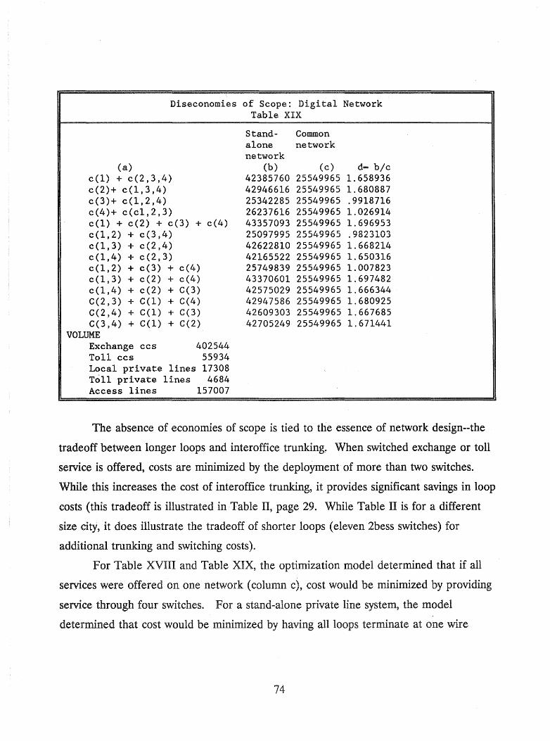
Diseconomies
(a) c(l) + c(2,3,4) c(2)+ c(1,3,4) c(3)+ c(1,2,4) c(4)+ c(c1,2,3) c(l) + c(2) + c(3) + c(4) c(1,2) + c(3,4) c(1,3) + c(2,4) c(1,4) + c(2,3) c(1,2) + c(3) + c(4) c(1,3) + c(2) + c(4) c(1,4) + c(2) + C(3) C(2,3) + C(l) + C(4) C(2,4) + C(l) + C(3) C(3,4) + C(l) + C(2)
VOLUME Exchange ccs 402544 Toll ccs 55934 Local private lines 17308 Toll private lines 4684 Access lines 157007
of Scope: Digital Network Table XIX
Stand- Common alone network network
(b) (c) d- b/c 42385760 25549965 1.658936 42946616 25549965 1.680887 25342285 25549965 .9918716 26237616 25549965 1.026914 43357093 25549965 1.696953 25097995 25549965 .9823103 42622810 25549965 1.668214 42165522 25549965 1.650316 25749839 25549965 1.007823 43370601 25549965 1.697482 42575029 25549965 1.666344 42947586 25549965 1.680925 42609303 25549965 1.667685 42705249 25549965 1.671441
The absence of economies of scope is tied to the essence of network design--the
tradeoff between longer loops and interoffice trunking~ When switched exchange or toll
service is offered, costs are minimized by the deployment of more than two switches.
While this increases the cost of interoffice trunking, it provides significant savings in loop
costs (this tradeoff is illustrated in Table II, page 29. While Table II is for a different
size city, it does illustrate the tradeoff of shorter loops (eleven 2bess switches) for
additional trunking and switching costs).
For Table XVIII and Table XIX, the optimization model determined that if all
services were offered on one network (column c), cost would be minimized by providing
service through four switches. For a stand-alone private line system, the model
determined that cost would be minimized by having all loops terminate at one wire
74
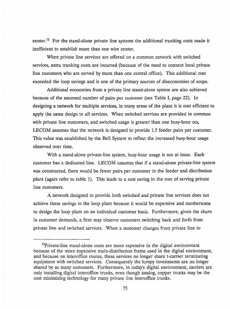
center.12 For the stand-alone private line systems the additional trunking costs made it
inefficient to establish more than one wire center.
When private line services are offered on a common network with switched
services, extra trunking costs are incurred (because of the need to connect local private
line customers who are served by more than one central office). This additional cost
exceeded the loop savings and is one of the primary sources of diseconomies of scope.
Additional economies from a private line stand-alone system are also achieved
because of the assumed number of pairs per cust0I11er (see Table I, page 22). In
designing a network for multiple services, in many areas of the plant it is cost efficient to
apply the same design to all services. When switched services are provided in common
with private line customers, and switched usage is greater than one busy-hour ccs,
LECOM assumes that the· network is designed to provide 1.5 feeder pairs per customer.
This value was established by the Bell System to reflect the increased busy-hour usage
observed over time.
With a stand-alone private-line system, busy-hour usage is not at issue. Each
customer has a dedicated line. LECOM assumes that if a stand-alone private-line system
was constructed, there would be fewer pairs per customer in the feeder and distribution
plant (again refer to table 1). This leads to a cost saving in the cost of serving private
line customers.
A network designed to provide both switched and private line services does not
achieve these savings in the loop plant because it would be expensive and cumbersome
to design the loop plant on an individual customer basis. Furthermore, given the churn
in customer demands, a firm may observe customers switching back and forth from
private line and switched services. When a customer changes from private line to
12Private-line stand-alone costs are more expensive in the digital environment because of the more expensive main-distribution frame used in the digital environment, and because on interoffice routes, these services no longer share t-carrier terminating equipment with switched services. Consequently the lumpy investments are no longer shared by as many customers. Furthermore, in today's digital environment, carriers are only installing digital interoffice trunks, even though analog, copper trunks may be the cost minimizing technology for many private line interoffice trunks.
75

switched services, the utility would want to have adequate plant available. Hence it
would choose to provide the higher value of feeder and distribution pairs to all
customers.
Two obvious interpretations can be made regarding our assumption that a stand
alone private line system would have fewer pairs per customer. First, it could be argued
that we are "fixing" the results. This assumption reduces the cost of private line stand
alone systems, and thereby increases the likelihood that we will conclude that the cost
function is not subadditive.
Our preferred interpratation is that an entrant will not always adopt the same
operating procedures as the incumbent, and LECOM merely reflects this possibility.13
These data suggest that to some extent bypass is the result of customers choosing
the cost minimizing service, rather than a local exchange carrier being unable to compete
due to regulatory barriers. Unless the local exchange carrier prices private line services
below its own marginal costs, the incumbent will be unable to price its service at a rate
below that of the entrants.
For the data reported on Table XVIII and Table XIX there were 22,044
customers per square mile. As indicated on Table V, page 34, this is in the range of
13We have assumed that an entant's annual carrying charge factors are equal to those of the incumbent. Teleport Communications has suggested that their operating costs for fiber optics are lower than those of the local exchange companies. "Comments of Teleport Communications Group," Federal Communications Commission Common Carrier Docket Number 91-141, August 6, 1991, pp.24-25. If Teleport's and other entrants costs are lower, LECOM's estimates of the cost of an alternative network may be overstated.
Teleport's position is supported by the position of Ameritech. In a study of the economics of bypass, Ameritech suggested that non-local exchange carriers production costs were approximately fifty percent lower than those of the Bell Operating Companies:
For all [bypass] systems, engineering and installation costs are based on ... Bell broad guage costs for underground [cable] ... However, these costs were reduced roughly 50% to account for lower competitive labor rates, engineering requirements, and loadings.
Ameritech submission to the Federal Communications Commission, October 2, 1984, "Effects of Access Pricing Policies on Customers of the Ameritech Companies," p.II-2.
76
customer density found in high density residential neighborhoods, and is considerably
lower than the number of customers per square mile found in high density business
district.
For less densely populated markets (customers per square mile), the industry may be
a natural monopoly.14 In the following tables, the density was only 4,051 per 'square
mile (slightly higher then the high end of the density found in districts dominated by
single family homes). With the lower density, economies of scope were present, and
This is so because customers are spread over a wider territory, cost savings are achieved
by having everyone on one network.
l~e qualifier "may" is used because we have only tested for the necessary condition for a natural monopoly.
77
Economies of Scope: Analog Network Table XX
(a) c(l) + c(2,3,4) c(2)+ c(1,3,4) c(3)+ c(1,2,4) c(4)+ c(c1,2,3) c(l) + c(2) + c(3) + c(4) c(1,2) + c(3,4) c(1,3) + c(2,4) c(1,4) + c(2,3) c(1,2) + c(3) + c(4) c(1,3) + c(2) + c(4) c(1,4) + c(2) + C(3) C(2,3) + C(l) + C(4) C(2,4) + C(l) + C(3) C(3,4) + C(l) + C(2)
VOLUME Exchange ccs 411,722 Toll ccs 68,821 Local private lines 15,395 Toll private lines 8,289 Access lines 154,348
Stand- Common alone network network
(b) (c) 40918797 26778053 41366189 26778053 28721087 26778053 29599307 26778053 46308878 26778053 29062391 26778053 41014819 26778053 40934163 26778053 31719585 26778053 44158386 26778053 43318232 26778053 43924809 26778053 43165311 26778053 43651684 26778053
78
(d) 1.528072 1.544780 1.072561 1.105357 1.729359 1.085306 1.531658 1.528646 1.184537 1.649051 1.617677 1.640329 1.611966 1.630129

Economies of Scope: Digital Network Table XXI
(a) c(l) + c(2,3,4) c(2)+ c(l,3,4) c(3)+ c(l,2,4) c(4)+ c(cl,2,3) c(l) + c(2) + c(3) + c(4) c(l,2) + c(3,4) c(1,3) + c(2,4) c(l,4) + c(2,3) c(1,2) + c(3) + c(4) c(l,3) + c(2) + c(4) c(1,4) + c(2) + C(3) C(2,3) + C(l) + C(4) C(2,4) + C(l) + C(3) C(3,4) + C(l) + C(2)
VOLUME Exchange ccs 411,722 Toll ccs 68,821 Local private lines 15,395 Toll private lines 8,289 Access lines 154,348
Stand- Common alone network network
(b) 53702766 53661205 34051102 34443464 58255836 34768326 53106496 53349818 37198886 55624677 55522443 56083211 55737655 55825277
(c) (d) 32408560 1.657055 32408560 1.655773 32408560 1.050682 32408560 1.062789 32408560 1.797545 32408560 1.072813 32408560 1.638656 32408560 1.646164 32408560 1.147811 32408560 1.716358 32408560 1.713203 32408560 1.730506 32408560 1.719844 32408560 1.722547
The data reported on Table XX and Table XXI show that in a less densely
populated market there are economies of scope. For both the digital and analog model
we find it is less expensive to construct one network that serves all customers [column
(c)], than construct multiple networks [column (b)].
In summary, the data reported in this section suggest that the coalition of
telecommunications users will minimize their production costs using only one network
when the customer density is low (for representative data on customer density, see page
33). In high customer density areas, the coalition is not stable and there is an economic
savings from constructing multiple networks.
79
If the Industry is Not a Natural Monopoly, What Does This Imply About the Need to Regulate the Industry?
We have argued in this chapter that in densely populated areas, the cost structure
exhibits diseconomies of scope. While this suggests that competition is feasible, these
results should not be used to argue that there is no longer a need to regulate the
industry. First, there are barriers to entry that limit the opportunity for entry into the
industry.15 Because of these barriers, it may be difficult for new firms to enter the
industry and provide service at a . lower cost than the incumbent firms. State regulatory
commissions can increase the extent to which the local market is contestable by
reviewing. and modifying the rules that govern the different services.
More importantly, at times when faced with entry, the Bell Operating Companies
have adopted rates that were based on the cost structure of their competitors.16 The
private line rates adopted in the 1960s (for example, Telpak) did not reflect the
incumbent's cost structure, and therefore may have been below their own cost of service.
In the future, the regulatory commissions need to determine the local exchange carriers
costs of providing private line services. If the local exchange carriers are allowed to set
rates below their marginal cost of service, inefficient production will result and entry will
be discouraged.
15David Gabel, "Deregulation: Should the Local Telephone Market Be Next?," New England Law Review 24 (1989): 39-61.
16Peter Temin, "Cross-Subsidies in the Telephone Network after Divestiture," Journal of Regulatory Economics 2 (December 1990): 353.
80
CHAPTER FIVE
ADDITIONAL ANALYSIS OF THE COST OF SERVICE
The Economics of Fiber Optics
LECOM can also be used to evaluate the economics of fiber optics in the local
loop and for interoffice trunking. The mechanics for this type of analysis, as well as our
Fiber Optics on Interoffice Trunks
In order to explore the extent to which fiber optics is the cost minimizing
technology for interoffice transport, we constructed the model to compare the cost of t
carrier on fiber and t-carrier on copper. In general the output from LECOM indicated
that t-carrier on copper was less expensive than t-carrier on fiber. This is consistent with
the wide-spread belief that the greatest economies from fiber are achieved on long-haul
routes (due in part to savings in repeater costs). On short-haul routes, these savings are
out-weighed by the additional cost of the multiplexer.
In order to study this issue the user of the model should select level 3 output (see
page 123). Data will be written to the file DIGIT AL.OUT which shows for each central
office the cost of using either t-carrier on copper or t-carrier on fiber. The model
calculates both costs and selects the technology that minimizes the annual cost of
production.
81
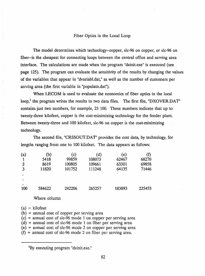
Fiber Optics in the Local Loop
The model determines which technology--copper, slc-96 on copper, or slc-96 on
fiber--is the cheapest for connecting loops between the central office and serving area
interface. The calculations are made when the program "dxinit.exe" is executed (see
page 125). The program can evaluate the sensitivity of the results by changing the values
of the variables that appear in "dvariabl.dat," as well as the number of customers per
Serving area (the first variable in "populatn.dat").
When LECOM is used to evaluate the economics of fiber optics in the local
loop,1 the program writes the results to two data files. The first file, "DXOVER.DAT'
contains just two numbers, for example, 23 100. These numbers indicate that up to
twenty-three kilofeet, copper is the cost-minimizing technology for the feeder plant.
Between twenty-three and 100 kilofeet, slc-96 on copper is the cost-minimizing
technology .
The second file, "CRSSOUT.DAT' provides the cost data, by technology,:for
lengths ranging from one to 100·kilofeet. The data appears as follows:
(a) 1 2 3
100
(b) 5418 8619
11820
584622
Where column
( a) = kilofeet
(c) 99859
100805 101752
242206
(d) 108073 109661 111248
265257
(b) = annual cost of copper per serving area
(e) 62467 63301 64135
183893
( c) = annual cost of slc-96 mode 1 on copper per serving area (d) = annual cost of slc-96 mode 1 on fiber per serving area (e) = annual cost of slc-96 mode 2 on copper per serving area (f) = annual cost of slc-96 mode 2 on fiber per serving area.
tBy executing program "dxinit.exe."
82
(f) 68270 69858 71446
225455

The data from "crssout.dat" can be imported to lotus and graphed. The following
two figures illustrate the crossover point for different technologies when either mode 1
or mode 2 subscriber line carrier is deployed.
The graph indicates that at approximately thirty-four ldlofeet, subscriber-line
carrier on copper is the technology of choice. For shorter length feeder pairs copper
wire should be deployed.
Figure 7 shows the economic tradeoff when mode 2 slc-96 is deployed. As with
the previous figure, the deployment of slc .. 96 raises the fixed cost of connecting a serving
area to the central office (as shown by the value of the y-intercept). On the other hand,
the slope of the curves associated with the slc-96 technology are flatter due to the lower
additional cost per kilofeet of cable. The slope for copper increases with distance
because for longer hauls more expensive, smaller gauge wire must be deployed (for
example, 19-9auge wire--see Table VI, and associated discussion).
The graph indicates that for the first twenty-three kilofeet, copper is the
technology of choice in the feeder plant. Beyond that distance, subscriber-line-carrier on
copper should be deployed.
Pricing
Effective regulation requires that commissions consider the cost of service when
establishing the prices for different services. While the primary purpose of this report
was to develop a cost model, some of the pricing implications of our cost study are
addressed below.2
Neoclassical economic theory argues that society's welfare will be maximized by
pricing products equal to the incremental (marginal) cost of production. The cost data
reported in Table XI through Table XVII suggest that the change from an analog to a
2See also David Gabel and Mark Kennet, "Pricing of Telecommunications Services," Review of Industrial Organization (forthcoming, 1992).
83

00 ~
Figure L I op: Copper v. SLC-96 Mode une
Thousands 300~i --------------------------------------
250 · ----------------------------- - ---------- -------------------------
200 · - ---- ---- - - - - -- - - ---- - - - --- - - - - - - -- -- -- - - ---- - - --- - - - -- -- - ...... - - -- - -- - - -------
1 50 J - - - - - - -
1 00 I ____ ~ / __ - - - - - - - - - - - ~ -.-: 0-- --~ ~ ~ --- :-"",:2:_
- - -
50 ' - ---------- ---------- - ------ -- ---------------------------------------
O~I---------------------------------------o 5 10 15 20 25 30 35 40 45 50
[--+- Copper - SLC on Copper - - SLC on Fiber ·1
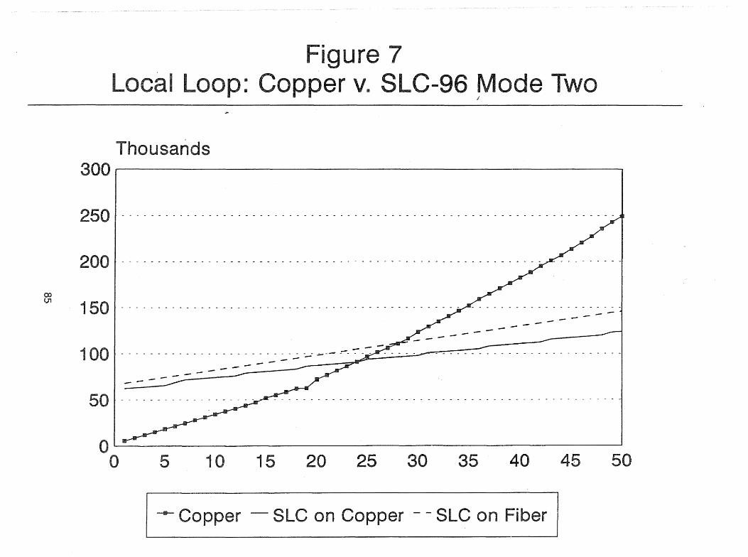
(X) U'1
Figure 7 Local Loop: Copper v. SLC-96 Mode Two
Thousands 300,~-----------------------------------------.
250 . --------------------------------------------------------------------
2 0 0 . ---------------------------------------------------------- ~- ---------
150 t - - - - - - - - - - - - - - - - - - - - - - - - - - - - - - - - - - - - - - - - - - - - -_-~- - - - - - - - - - -_- ~ -~ __ - :.. -..: -
- -- -100 L -~ r - - .. - - - - - - - .. - .-.- -....", ~- .. .... ........ .. .. .. .. .. .. .. .. .. .. .. .. .. .. .. .. - - .. .. .. .. .. .. ..
---~ - -- - --- - - - -
50 · - --- ------- -------- ....... - - - -- - --- -- - -- - -- -- - -- --- ---- - -- -- ---- -- --------
o 1-
o 5 10 15 20 25 30 35 40 45 50
[ -- ~~~~~r -SLC on Copper - - SLC on Fiber [
digital environment raises the marginal cost of switched access and local and toll private
line services. On the other hand, the incremental cost of exchange and toll switched
services decline.
If prices during the analog era of telephony had equalled the incremental cost of
production, the results from the digital cost model suggest a need to lower the price of
switched services and raise the price of private line and switched access services. Before
a more definitive statement can be made, a more detailed study of current prices must
be undertaken.
Furthermore, while basic microeconomic theory argues that welfare is maximized
by setting price equal to the marginal cost of production, theory also argues that this
condition holds under restrictive conditions. Because of the externalities associated with
telephone service, and because quality as well as quantity affects the cost of service,
welfare will not be maximized by setting prices equal to the incremental costs of
production.
While the role of externalities is well known, there has been a limited discussion
of the role of quality in pricing telecommunication services. Economic theory stresses
that to maximize society's welfare, basic telephone service should only bear a portion of
the cost of upgrading the network to satisfy the more stringent requirements of nonbasic
services. The additional charges to basic services should be based on the value of the
improved, plain-old-telephone service.3
The incremental cost data reported in Table XI through Table XVII well
illustrate this issue. Replacing analog with digital facilities improves the local exchange
companies' ability to offer data and other enhanced services. The operation of the
digital network requires that the analog voice signals spoken into the telephone
transmitter be converted to digital signals. This analog-digital conversion is not required
where analog facilities are used.
3Michael Spence, "Monopoly, Quality and Regulation," Bell Journal of Economics 6 (1975): 417-29; and Sickler, J. "A Theory of Telephone Rates," Journal of Land and Public Utility Econo'?1ics 4, 177 (1928).
86

Since each switched access line must be equipped with an analogi digital
converter, the cost of access is increased [see page 61 through 67, row "INCREMENTAL
COST SWITCH ACCESS UNE (LOOP)"]. The telephone companies are willing to
incur this additional cost because, once it is made, the cost of providing other services is
reduced.
Since the divestiture of AT&T, the industry'S pricing trend has been to recover
the cost of switched access in the price of exchange service.4 Using the cost data from
Table XIV, page 64, and assuming that the busy-hour usage per customer is 3.5 ccs, the
change from the analog to digital environment raises the total cost of access and
switched exchange service by $34.55 ($125.045 - $90.495, see Table XXII).
Impact of Digital Technology on the Annual Cost of Providing Access and Exchange Services
Table XXII
Access Usage @3.5 ccs Total Cost
Analog network $51.12 11.25*3.5 = 51.12 + 39.375 == 39.375 90.495
Digital network 112.69 3.53*3.5 == 112.69 + 12.355 12.355 == 125.045
If the price of exchange service equals the incremental cost of access and
exchange usage, the price of the service would increase over 30 percent. Since digital
technology has little or no impact on the quality of exchange voice switched service, the
welfare of subscribers to plain-old-telephone service would be reduced. To maximize
society's welfare, plain-old telephone service subscribers should not be required to pay
for improvements that provide little or no benefit.
4F ederal Communications Commission, Third Report and Order, CC Docket No. 78-72, Phase I, December 22, 1982.
87

CHAPTER SIX
CONCLUSION AND SOME FUTURE USES FOR THE MODEL
Identified below are some areas where analysts may find it useful to use our cost
model:
1. Calculating the long-run marginal cost of access, private line, exchange, and toll services.
2. Calculating the stand-alone cost of private line, toll, and exchange services. 3. Measuring the degree to which the industry is a natural monopoly. 4. Quantifying the impact of replacing analog with digital technology. 5. Quantifying the affect of different "fill" rates in the local loop. 6. Identifying the conditions were it is economical to deploy fiber optics in the
local loop and on interoffice trunks. 7. Forecasting the future topology of the network.
These applications are described more fully below.
Marginal Cost of Service
In appendix one we report our econometric estimates of the cost function. The
marginal cost of the different services can be derived by working with the estimated
parameters of the cost function.
We have also shown that the marginal cost of different services can be derived
directly from LECOM. In Table XI through Table XVII we provided comparative
results from the digital and analog model.
In appendix two we have provided work sheets and instructions that will allow the
user to estimate the marginal cost of toll and exchange busy-hour ccs, local and toll
private-line as well as switched access services.
Calculating the Stand-Alone Cost of Service
The model may be used to calculate the stand-alone cost for private line, toll, and
exchange services. The stand-alone cost provides a bench mark of the maximum
revenues that can be collected from a service in a contestable market. If the revenues
for a service are larger than the stand-alone cost, the users of the service have an
89
economic incentive to establish a private network. The stand-alone cost of a service is
obtained by setting the level of all other services equal to zero.1
Natural Monopoly
In Table XVIII through Table XXI we have shown how the data from the
LECOM can be used to test if the industry is a natural monopoly. We have provided an
example where high customer density markets may find it less expensive to have two
firms supply service than one. We aiso have shown that in a less densely populated city
the cost of production may be minimized when only one firm supplies local
telecommunication services.
Analog v. Digital Technologies
There has been considerable debate in the industry over the economics of
replacing analog with digital switching. Since we have developed separate optimization
models for the analog and digital environment, a tool is now available to compare the
relative advantages of both technologies.
These advantages can be ascertained either by working with the statistical cost
function or by running LECOM. The statistical cost function provides a convenient
estimate of the difference in the cost of service attributable to a change in technology.
Alternatively, LECOM can provide the data for the comparison. Table XI
through Table XVII show the total and marginal cost of service under the assumption of
analog and digital technology. In general, replacing analog with digital technology raises
the total cost of service, lowers the cost of switched toll and exchange services, and raises
the cost of providing private line services and switched access.
IFor example, the stand-alone cost of an exchange network is estimated by setting the percent of toll usage and the percent of private line loops equal to zero (see subdirectory varfiles, file variable.317. This file was generated by the work sheet stadalone.wkl, subdirectory 10tus22).
90

Effect of Fill on the Cost of Service
The model can be used to identify the cost impact of various fill (utilization)
levels. For example, the user of the model can vary the fill factor on outside plant in
the local loop through variables "LOOPUTIL" (maximum percent cable fill),
"FPPERCUST' (feeder pairs per customer), "DPPERCUST' (distribution paris per
customer), and "FPSLCPERCUST' (feeder communication channels per customer served
by SLC-96®). In the switch, the effect of different fill factors can be evaluated through
variable "SWITCHUTIL." For interoffice facilities, variable "TUTIL" allows the user to
study the effect of varying fill factors on t-carrier systems.
Economics of Fiber Optics
As discussed earlier the optimization model can be used to evaluate the cost
savings available by using fiber optics for interoffice trunks or the local loop. In our
study, in general, t-carrier on copper was less expensive than t-carrier on fiber.
Forecasting the Future Network Topology
The model can be used to evaluate how new technology will effect the network's
topology. The results reported in tables XI through XVII suggest that replacing analog
with digital switches will lead to an increase in the number of switches, and offers no
clear pattern in the length of the local loop.
91


APPENDIX ONE
ECONOMETRIC RESULTS
Summarizing the results of repeated simulations of our cost model using the
traditional translog estimation of Christensen, Jorgenson, and Lau (1973) provides a
number of insights into the advantages of the process model approach. The ttanslog cost
function is given by
C(W,y)
where:
p
= «0 + E i=l
w = P-vector of the natural logarithms of factor prices;
y = Q-vector of the natural logarithms of outputs;
z = R-vector of other cost factors and their interactions;
a o = constant;
a, P, y, a, p,A estimable parameters;
and
€ = disturbance term.
93

It is useful here to recall that the translog function can be regarded as a second
order Taylor expansion in logs which approximates the true underlying cost function.
Thus, the disturbance term is simply an error resulting from the imprecision of the fit of
the quadratic approximation, and not a stochastic unobservable as is often assumed.
Among the useful properties of the translog function is the fact that it is in
principle possible to test various results from production theory, among which is
homogeneity of degree 1 in prices. The homogeneity restrictions and the related
symmetry restrictions are
and
p
E (Xi = 1; i=l
p
E Y ij = 0; j=l
p
E P ij = 0; i=l
Y ij = Y ji·
Table E-1 gives results for the restricted and unrestricted translog estimation for
both analog and digital technology. All price and output variables have the expected
sign in both models for both technologies. The mean and standard deviation of the
variables are reported in table E-5. Variable mnemonics are as follows.
94

Variable Mnemonics Constant:
CONST constant Price variables--first order terms:
PRICELAB price of labor PRICECAP price of capital PRICEMAT price of materials
Price variables--squared values: PL2 PRICELAB * PRICELAB PK2 PRICECAP * PRICE CAP PM2 PRICEMAT * PRICEMAT
Output variables--first order terms: ACCLINE access lines EXCCSEC hundreds of exchange busy-hour calling seconds TLCCSEC hundreds of toll busy-hour calling seconds LCPLCUST local private lines TLPLCUST toll private lines
Output variables--squared values AL2 ACCLINE * ACCLINE (ACCLINE squared) EXC2 EXCCSEC * EXCCSEC TLC2 TLCCSEC * TLCCSEC LPL2 LCPLCUST * LCPLCUST TPL2 TPLCUST * TPLCUST
Geographical Size of the Market: AREA area of the city in square kilofeet AR2 AREA * AREA (AREA squared)
Interaction terms: ARPK AREA * PRICECAP ARPL ARPM ARAL AREXCCS ARTLCCS ARPLP ARTPL PKPL PKPM PKAL PKEXCCS PKTLCCS PKLPL PKTPL PLPM PLAL PLEXCCS PLTLCCS PLLPL PLTPL PMAL PMEXCCS PMTLCCS PMLPL PMTPL
AREA * PRICELAB AREA * PRICEMAT AREA * ACCLINES AREA * EXCHCCS AREA * TLCCSEC AREA * LCPLCUST AREA * TPLCUST PRICECAP * PRICELAB PRICECAP * PRICEMAT PRICECAP * ACCLINES PRICECAP * EXCHCCS PRICECAP * TLCCSEC PRICECAP * LCPLCUST PRICECAP * TLPLCUST PRICELAB * PRICEMAT PRICELAB * ACCLINES PRICELAB * EXCHCCS PRICELAB * TLCCSEC PRICELAB * LCPLCUST PRICELAB * TLPLCUST PRICEMAT * ACCLINES PRICEMAT * EXCHCCS PRICEMAT * TLCCSEC PRICEMAT * LCPLCUST PRICEMAT * TPLCUST
95
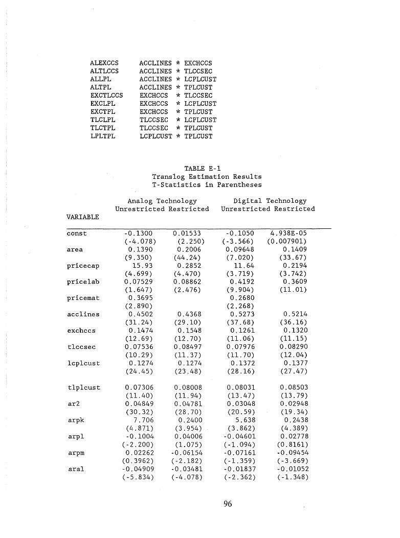
ALEXCCS ACCLINES * EXCHCCS ALTLCCS ACCLINES * TLCCSEC ALLPL ACCLINES * LCPLCUST ALTPL ACCLINES * TPLCUST EXCTLCCS EXCHCCS * TLCCSEC EXCLPL EXCHCCS * LCPLCUST EXCTPL EXCHCCS * TPLCUST TLCLPL TLCCSEC * LCPLCUST TLCTPL TLCCSEC * TPLCUST LPLTPL LCPLCUST * TPLCUST
TJl...BLE E-l Trans10g Estimation Results T-Statistics in Parentheses
Analog Technology Digital Technology Unrestricted Restricted Unrestricted Restricted
VARIABLE
const -0.1300 0.01533 -0.1050 4.938E-05 (-4.078) (2.250) (-3.566) (0.007901)
area 0.1390 0.2006 0.09648 0.1409 (9.350) (44.24) (7.020) (33.67)
pricecap 15.93 0.2852 11.64 0.2194 (4.699) (4.470) (3.719) (3.742)
price lab 0.07529 0.08862 0.4192 0.3609 (1.647) (2.476) (9.904) (11.01)
pricernat 0.3695 0.2680 (2.890) (2.268)
acc1ines 0.4502 0.4368 0.5273 0.5214 (31.24) (29.10) (37.68) (36.16)
exchccs 0.1474 0.1548 0.1261 0.1320 (12.69) (12.70) (11.06) (11.15)
t1ccsec 0.07536 0.08497 0.07976 0.08290 (10.29) (11.37) (11.70) (12.04)
1cp1cust 0.1274 0.1274 0.1372 0.1377 (24.45) (23.48) (28.16) (27.47)
t1p1cust 0.07306 0.08008 0.08031 0.08503 (11.40) (11.94) (13.47) (13.79)
ar2 0.04·849 0.04781 0.03048 0.02948 (30.32) (28.70) (20.59) (19.34)
arpk 7.706 0.2400 5.638 0.2438 (4.871) (3.954) (3.862) (4.389)
arp1 -0.1004 0.04006 -0.04601 0.02778 (-2.200) (1.075) (-1.094) (0.8161)
arprn 0.02262 -0.06154 -0.07161 -0.09454 (0.3962) (-2.182) (-1.359) (-3.669)
aral -0.04909 -0.03481 -0.01837 -0.01052 (-5.834) (-4.078) (-2.362) (-1.348)
96

arexccs 0.01014 0.007430 0.007762 0.007756 (1.760) (1.233) (1.436) (1.388)
art1ccs -0.007463 -0.01223 -0.01967 -0.02089 (-1.809) (-2.906) (-5.142) (-5.417)
ar1p1 ·0.02068 -0.02413 0.001921 -4.856E-05 (-3.738) (-4.390) (.3747) (-0.009647)
artp1 -0.01799 -0.01905 -0.009905 -0.01086 (-4.683) (-5.042) (-2.782) (-3.137)
pk2 0.6741 -0.1962 0.9344 -0.1899 (1.526) (-1.007) (2.289) (-1.068)
pkp1 1.247 -0.5959 0.5057 -0.3261 (1.951) (-3.048) (0.8587) (-1.827)
pkpm 3.328 -0.8394 3.273 -0.7227 (2.449) (-5.794) (2.606) (-5.463)
pka1 0.3724 0.1318 0.3222 0.1413 (5.882) (2.548) (5.493) (2.976)
pkexccs -0.01116 -0.06034 0.03803 -0.07440 (-0.2668) (-2.477) (.9833) (-3.342)
pkt1ccs -0.03682 -0.08261 -0.008023 -0.07507 (-0.8555) (-3.005) (-0.2017) (-2.989)
pk1p1 -0.001226 -0.04045 -0.04524 -0.09002 (-0.02702) (-1.522) (-1.079) (-3.709)
pktp1 -0.2216 -0.2012 -0.2304 -0.1915 (-4.759) (-5.301) (-5.357) (-5.526)
p12 -0.4852 -0.6561 -0.2065 -0.6156 (-2.252) (-4.054) (-1.038) (-4.167)
p1pm 1.728 -0.1177 -0.1994 -0.1429 (2.011) (-1.018) (-0.2513) (-1.355)
pIal 0.05141 -0.1036 -0.008273 -0.09945 (0.9707) (-2.039) (-0.1677) (-2.122)
p1exccs 0.1160 0.01155 0.1239 0.05417 (2.92) (0.3846) (3.370) (1.958)
p1t1ccs -0.1817 -0.1044 -0.08295 -0.04473 (-6.375) (-0.030) (-3.133) (-1.878)
p11p1 -0.02375 -0.05869 -0.02172 -0.008901 (-0.6519) (-1.812) (-0.6456) (-0.3008)
p1tp1 0.1060 -0.06982 0.04190 -0.06684 (2.459) (-2.569) (1.054) (-2.694)
pm2 0.8332 0.5526 (5.087) (3.652)
pma1 -0.02469 -0.03645 (-0.4044) -(.6458)
pmexccs 0.005688 0.04304 (0.09828) (.8048)
pmt1ccs 0.1371 0.1155 (2.62) (2.390)
pmlp1 0.1015 0.07677 (1.800) (1.474)
97
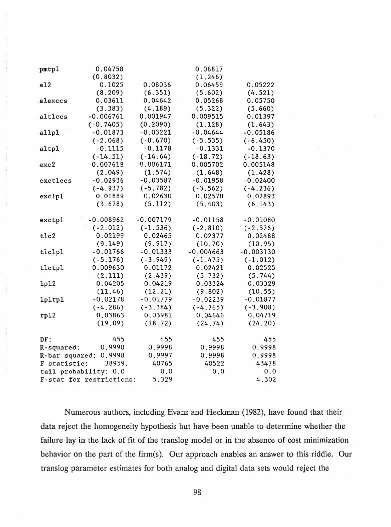
pmtp1 0.04758 0.06817 (0.8032) (1.246)
a12 0.1025 0.08036 0.06459 0.05222 (8.209) (6.351) (5.602) (4.521)
a1exccs 0.03611 0.04642 0.05268 0.05750 (3.383) (4.189) (5.322) (5.660)
a1t1ccs -0.006761 0.001947 0.009515 0.01397 (-0.7405) (0.2090) (1.128) (1.643)
allp1 ·0.01873 -0.03221 -0.04644 -0.05186 (-2.068) (-0.670) (-5.535) (-6.450)
altp1 -0.1115 -0.1178 -0.1331 -0.1370 ( .. 14.51) (-14.64) (-18.72) (-18.63)
e ........ 1) ......... " () ()()7~1R v. ,,'-' I v..a.."" 0.006171 0.005702 0.005148
(2.049) (1.574) (1.648) (1.428) exct1ccs -0.02936 -0.03587 -0.01958 -0.02400
(-4.937) (-5.782) (-3.562) (-4.236) exc1pl 0.01889 0.02630 0.02570 0.02893
(3.678) (5.112) (5.403) (6.143)
exctpl -0.008962 -0.007179 -0.01158 -0.01080 (-2.012) (-1.536) (-2.810) (-2.526)
t1c2 0.02199 0.02465 0.02377 0.02488 (9.149) (9.917) (10.70) (10.95)
t1c1p1 -0.01766 -0.01333 -0.004663 -0.003130 (-5.176) (-3.949) (-1.475) (-1.012)
tlctp1 0.009630 0.01172 0.02421 0.02525 (2.111) (2.439) (5.732) (5.744)
lp12 0.04205 0.04219 0.03324 0.03329 (11.46) (12.21) (9.802) (10.55)
1pltp1 -0.02178 -0.01779 -0.02239 -0.01877 (-4.286) (-3.384) (-4.765) (-3.908)
tp12 0.03863 0.03981 0.04646 0.04719 (19.09) (18.72) (24.74) (24.20)
DF: 455 455 455 455 R-squared: 0.9998 0.9998 0.9998 0.9998 R-bar squared: 0.9998 0.9997 0.9998 0.9998 F statistic: 38959. 40765 40522 43478 tail probability: 0.0 0.0 0.0 0.0 F-stat for restrictions: 5.329 4.302
Numerous authors, including Evans and Heckman (1982), have found that their
data reject the homogeneity hypothesis but have been unable to determine whether the
failure lay in the lack of fit of the translog model or in the absence of cost minimization
behavior on the part of the firm(s). Our approach enables an answer to this riddle. Our
translog parameter estimates for both analog and digital data sets would reject the
98

homogeneity and symmetry hypothesis at any reasonable level of significance. However,
the raw data suggests that the cost function is homogeneous. Performing the experiment
of doubling prices at varying levels of output gives us the result that cost doubles
consistently. Table E-2 reports the results of the experiment. Although we would need
to perform this experiment more times with scalar multiples other than 2 to draw firm
conclusions, the results shown are strongly suggestive: the unrestricted translog cost
function seems to be a poor approximation to the true cost function in that it fails to
capture the homogeneity property.
TABLE E-2 Homogeneity Experiment Results
ANALOG RUNS
Experiment Cost at Cost at run 2 x base Computed number price price multiple
1 22869521 11389766 2.0079 2 13401533 6700767 2.0000 3 79614019 40031981 1.9887 4 35112968 17269047 2.0332 5 2481061 1240531 1.9999 6 39536617 19930502 1.9837 7 32255607 16102487 2.0031 8 11453032 5727779 1.9995
DIGITAL RUNS
1 25303515 12828382 1.9724 2 17794843 8897422 2.0000 3 89641129 43487947 2.0612 4 40408481 20207034 1.9997 5 3663404 1831702 2.0000 6 44579706 22116003 2.0157 7 42422396 21211198 2.0000 8 15970583 7985291 2.0000
The Evans and Heckman (1982) paper also reports another common problem,
one which partly inspired this research. It is difficult to find orthogonal nonexperimental
data for the telecommunications industry (or many other industries, for that matter).
99
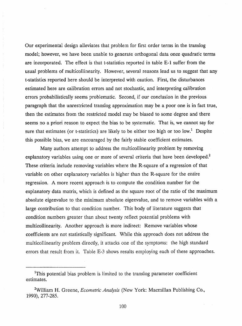
Our experimental design alleviates that problem for first order terms in the translog
model; however, we have been unable to generate orthogonal data once quadratic terms
are incorporated. The effect is that t-statistics reported in table E-1 suffer from the
usual problems of multicollinearity. However, several reasons lead us to suggest that any
t-statistics reported here should be interpreted with caution. First, the disturbances
estimated here are calibration errors and not stochastic, and interpreting calibration
errors probabilistically seems problematic. Second, if our conclusion in the previous
paragraph that the unrestricted translog approximation may be a poor one is in fact true,
then the estimates from the restricted model may be biased to some degree and there
seems no a priori reason to expect the bias to be systematic. That is, we cannot say for
sure that estimates (or t-statistics) are likely to be either too high or too low. l Despite
this possible bias, we are encouraged by the fairly stable coefficient estimates.
Many authors attempt to address the multicollinearity problem by removing
explanatory variables using one or more of several criteria that have been developed.2
These criteria include removing variables where the R-square of a regression of that
variable on other explanatory variables is higher than the R-square for the entire
regression. A more recent approach is to compute the condition number for the
explanatory data matrix, which is defined as the square root of the ratio of the maximum
absolute eigenvalue to the minimum absolute eigenvalue, and to remove variables with a
large contribution to that condition number. This body of literature suggests that
condition numbers greater than about twenty reflect potential problems with
multicollinearity. Another approach is more indirect: Remove variables whose
coefficients are not statistically significant. While this approach does not address the
multicollinearity problem directly, it attacks one of the symptoms: the high standard
errors that result from it. Table E-3 shows results employing each of these approaches.
IThis potential bias problem is limited to the translog parameter coefficient estimates.
2William H. Greene, Ecometric Analysis (New York: Macmillan Publishing Co., 1990), 277-285.
100

However, for the remainder of this discussion, we will not use these results but rather
those in tables B-1 and E-4, where it is possible to impose the homogeneity/symmetry
restrictions; it is not possible to impose these restrictions when variables are removed.
TABLE E-3 Analog Trans10g Estimates With Interaction Terms Removed
According to Various Criteria
VARIABLE
const
area
pricecap
price lab
pricemat
acc1ines
exchccs
t1ccsec
1cp1cust
t1p1cust
ar2
arpk
arp1
arpm
ara1
art1ccs
ar1p1
artp1
pkp1
T-Ratios in Parentheses
Significance Partial Condition Number Criterion
-0.1076 (-6.445)
0.1428 (16.95)
13.96 (8.253) 0.09133
(2.956) 0.2933
(13.18) 0.4395
(35.02) 0.1513
(16.44) 0.08741
(14.91) 0.1240
(25.03) 0.07887
(13.16) 0.04903
(34.74) 6.799
(8.216) -0.1182
(-4.706)
-0.03260 (-5.476)
-0.008249 (-2.198) -0.02575 (-5.153) -0.01916 (-5.635)
1.880
Correlation Criterion
0.02207 (3.797) 0.2047
(50.71) 0.07150
(1.108) 0.1996
(6.684) 0.3694
(17.08) 0.4335
(32.38) 0.1567
(15.97) 0.09187
(14.73) 0.1189
(22.64) 0.08215
(12.85)
0.04908 (32.55)
.009519 (0.4516)
-0.03023 (-4.757) -0.01144 (-2.868) -0.02761 (-5.176) -0.01688 (-4.662)
-0.9879
101
0.3084 (27.42) 0.2047
(24.21) -0.7234
(-4.671) 0.2515
(2.267) -0.07470
(-0.5330) 0.5903
(19.54) -0.1077
(-6.504) -0.007970
(-0.7123) 0.04860
(4.609) 0.2492
(25.41)
0.5974 (11.11) 0.5237
(6.922)
-0.6574
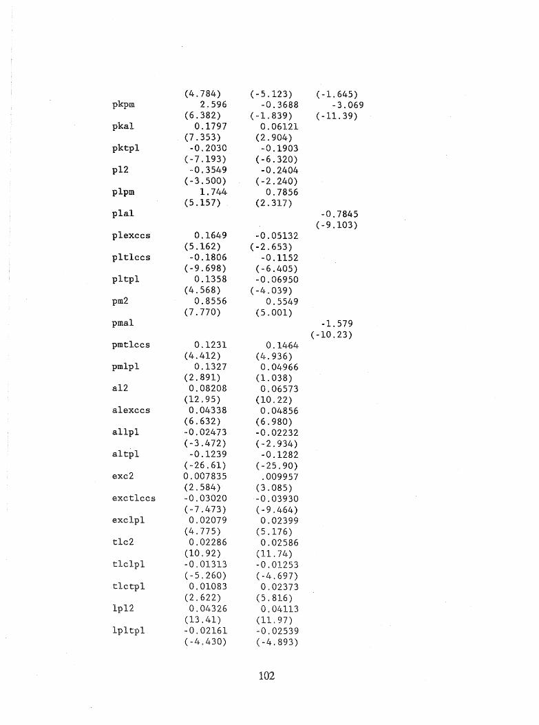
(4.784) (-5.123) (-1.645) pkpm 2.596 -0.3688 -3.069
(6.382) (-1.839) (-11.39) pka1 0.1797 0.06121
(7.353) (2.904) pktp1 -0.2030 -0.1903
(-7.193) (-6.320) p12 -0.3549 .. 0.2404
(-3.500) ( .. 2.240) p1pm 1.744 0.7856
(5.157) (2.317) p1a1 -0.7845
(-9.103) p1exccs 0.1649 .. 0.05132
(5.162) (-2.653) p1t1ccs -0.1806 -0.1152
(-9.698) (-6.405) p1tp1 0.1358 -0.06950
(4.568) (-4.039) pm2 0.8556 0.5549
(7.770) (5.001) pma1 -1.579
(-10.23) pmt1ccs 0.1231 0.1464
(4.412) (4.936) pm1p1 0.1327 0.04966
(2.891) (1.038) a12 0.08208 0.06573
(12.95) (10.22) a1exccs 0.04338 0.04856
(6.632) (6.980) a11p1 -0.02473 -0.02232
(-3.472) (-2.934) a1tp1 -0.1239 -0.1282
(-26.61) (-25.90) exc2 0.007835 .009957
(2.584) (3.085) exctlccs -0.03020 -0.03930
(-7.473) (-9.464) exclp1 0.02079 0.02399
(4.775) (5.176) t1c2 0.02286 0.02586
(10.92) (11.74) tlclp1 -0.01313 -0.01253
(-5.260) (-4.697) t1ctp1 0.01083 0.02373
(2.622) (5.816) 1p12 0.04326 0.04113
(13.41) (11.97) 1p1tp1 -0.02161 -0.02539
(-4.430) (-4.893)
102

tp12 0.04026 0.04000 (22.33) (20.77)
OF: 468 469 493 R-squared: 0.9998 0.9997 0.9769 R-bar squared: 0.9998 0.9997 0.9762 F statistic: 49954 44843 1304 tail probability: 0.0 0.0 0.0
Table E-4 presents results when access lines are not treated as an output. This
exclusion results from a debate between regulators and telephone company economists;
the companies maintain that access to the telephone network should be treated as a
separate output, while many regulators doubt if customers place any value on a "product"
which, by itself, is useless. Again we report unrestricted and restricted estimates, where
the restriction refers to homogeneity and symmetry implied by cost minimization.
TABLE E-4 Trans10g Estimates With Access Lines Not Treated as a Product
T-Statistics in Parentheses
Analog Technology Digital Technology Unrestricted Restricted Restricted Unrestricted Restricted Restricted
(density) (density) (no ACCLINE) (density) (density) (no ACCLINE)
const -0.01738 -0.01741 0.01513 -0.04330 -0.04272 -9.016E-05 (-0.9891) (-1.004) (2.249) (-2.336) (-2.326) (-0.01455)
area 0.2046 0.1438 (44.44) (33.68)
pricecap -1.441 0.1971 0.1428 -1.670 0.05628 0.1152 (-3.039) (1.218) (1.933) (-3.362) (0.3299) (1.691)
price1ab -0.05866 0.2068 0.08504 0.1475 0.4083 0.3583 (-0.4032) (2.270) (2.407) (0.9618) (4.244) (11.02)
pricemat 0.5904 0.5781 (1.412) (1.320)
acc1ines -0.1128 -0.1219 0.4445 -0.04900 -0.05888 0.5272 (-9.183) (-10.31) (29.72) (-3.811) (-4.742) (36.52)
exchccs 0.6750 0.6766 0.1492 0.6840 0.6880 0.1278 (33.10) (33.67) (12.30) (31.68) (32.25) (10.80)
t1ccsec 0.1564 0.1356 0.08212 0.1482 0.1215 0.08081 (7.222) (6.616) (11.07) (6.478) (5.585) (11.77)
lcp1cust 0.08678 0.08824 0.1258 0.1000 0.1029 0.1365 (5.133) (5.220) (23.41) (5.595) (5.735) (27.36)
t1p1cust 0.1554 0.1532 0.07812 0.1550 0.1522 0.08360 (7.972) (7.829) (11.77) (7.526) (7.337) (13.63)
103

ar2 0.04774 0.02942 (29.04) (19.46)
arpk 0.1602 0.1854 (2.516) (3.165)
arp1 0.04990 0.03498 (1.353) (1.033)
arpm -0.1337 -0.1473 (-3.929) (-4.717)
ara1 -0.04248 -0.01613 (-4.896) (-2.024)
arexccs 0.008672 0.008650 (1.456) (1.558)
artlccs -0.009668 =0.01901 (-2.296) (-4.901)
ar1p1 -0.02224 0.001332 (-4.083) (0.2656)
artp1 -0.01824 ·0.01026 (-4.885) (-2.984)
pk2 -2.216 -1.022 0.005240 -2.117 -1.269 -0.04230 (-2.221) (-2.056) (0.02623) (-2.024) (-2.426) (-0.2306)
pkp1 1.587 0.1995 -0.7219 1.918 0.5770 -0.4183 (1.109) (0.4515) (-3.685) (1.279) (1.243) (-2.327)
pkpm -2.401 -0.09305 -0.6969 -2.007 -0.03360 -0.6183 (-1.240) (-0.2348) (-4.706) (-0.9899) (-0.08051) (-4.549)
pka1 -0.2076 -0.3860 0.2329 -0.2069 -0.4320 0.2154 (-1.485) (-3.053) (4.019) (-1.412) (-3.248) (4.033)
pkexccs -0.2617 -0.1765 ·0.07822 -0.2785 -0.2152 -0.08751 (-2.415) (-2.536) (-3.191) (-2.453) (-2.939) (-3.885)
pkt1ccs 0.05181 0.1367 -0.1013 0.08064 0.1376 -0.08876 (0.4376) (1.822) (-3.671) (0.6503) (1.744) (-3.503)
pk1p1 -0.4325 -0.1936 -0.05185 -0.5099 -0.2538 -0.09836 (-3.381) (-2.587) (-1.964) (-3.804) (-3.227) (-4.058)
pktp1 -0.2505 0.1248 -0.2124 -0.2862 0.1307 -0.1996 (-1.710) (1.427) (-5.652) (-1.865) (1.421) (-5.790)
p12 -1.262 -0.4378 -0.7125 -1.162 -0.3861 -0.6568 (-1.923) (-0.9128) (-4.442) (-1.692) (-0.7662) (-4.462)
p1pm 1.621 -0.5199 -0.2914 0.6582 -0.4854 -0.2702 (0.6311) (-1.437) (-2.361) (0.2448) (-1.276) (-2.386)
pIal 0.1047 0.01334 ·0.05484 0.1093 0.03564 -0.06391 (1.014) (0.1575) (-1.058) (1.009) (0.4002) (-1.331)
plexccs 0.04669 0.04734 -0.02280 0.04409 0.07555 0.02908 (0.5921) (0.9745) (-0.7344) (0.5315) . (1.469) (1.012)
p1t1ccs -0.2243 -0.1936 -0.1156 -0.1643 -0.1605 -0.05286 (-3.032) (-3.750) (-4.490) (-2.117) (-2.951) (-2.222)
p11p1 0.01817 -0.05780 -0.06399 0.05966 ·0.01038 -0.01279 (0.1765) (-0.6768) (-2.000) (0.5528) (-0.1157) (-0.4356)
p1tpl -0.03365 -0.08741 -0.08635 -0.04417 -0.06661 -0.07894 (-0.3511) (-1.268) (-3.176) (-0.4393) (-0.9168) (-3.164)
pm2 0.8170 0.6962 (1.547) (1.258)
pmal 0.1661 0.1697 0.1116 0.1796 0.1832 0.06052
104

(0.9955) (1.809) (2.030) (1.028) (1.858) (1.199) pmexccs 0.1009 0.1138
(0.5852) (0.6298) pmt1ccs 0.1806 0.2157
(1.052) (1.199) pm1p1 0.1555 0.1457
(0.8131) (0.7270) pmtp1 0.05095 0.04191
(0.2562) (0.2012) a12 0.05547 0.05492 0.08923 0.03786 0.03698 0.05871
(11.5'2) (11.38) (7.018) (7.500) (7.280) (5.033) a1exccs -0.08966 -0.08738 0.04266 -0.09020 -0.08899 0.05476
(-10.59) (-10.67) ,(3.884) (-10.11) (-10.27) (5.412) a1t1ccs 0.04595 0.04574 -0.003239 0.06373 0.06323 0.01019
(4.896) (4.992) (-0.3483) (6.469) (6.549) (1.194) a11p1 -0.005365 -0.004878 -0.02182 -0.03314 -0.03186 -0.04424
(-0.3495) (-0.3343) (-2.397) (-2.057) (-2.072) (-5.277) a1tp1 0.06756 0.06204 -0.1148 0.06396 0.05736 -0.1348
(6.255) (6.033) (-14.39) (5.648) (5.301) (-18.39) exc2 0.1045 0.1064 0.007067 0.1102 0.1124 0.005797
(.17.73) (18.33) (1.824) (17.74) (18.29) (1.618) exct1ccs -0.01899 -0.03888 -0.03398 -0.01223 -0.03429 -0.02262
(-1.582) (-3.486) (-5.532) (-0.9716) (-2.921) (-4.011) exc1p1 " -0.02324 -0.01693 0.02102 -0.01826 -0.01087 0.02506
(-2.670) (-1.957) (3.985) (-1.994) (-1.190) (5.163) exctp1 -0.02553 -0.02618 -0.008318 -0.03119 -0.03201 -0.01164
(-3.064) (-3.129) (-1.800) (-3.561) (3.625) (-2.739) t1c2 0.03213 0.03053 0.02438 0.03006 0.02773 0.02467
(5.196) (4.966) (9.933) (4.623) (4.274) (10.95) t1c1p1 -0.004332 -0.004984 -0.01678 0.009912 0.009070 -0.005656
(-0.5707) (-0.6637) (-4.849) (1.245) (1.148) (-1.775) t1ctp1 -0.05101 -0.03876 0.01222 -0.03997 -0.02700 0.02560
(-3.807) (-2.929) (2.577) (-2.844) (-1.937) (5.870) 1p12 0.03477 0.03150 0.04179 0.02614 0.02316 0.03299
(2.956) (2.949) (12.25) (2.120) (2.061) (10.53) 1p1tp1 -0.07654 -0.07901 -0.01963 -0.08960 -0.09192 -0.02012
(-4.800) (-4.972) (-3.767) (-5.348) (-5.483) (-4.203) tp12 0.07940 0.07585 0.03940 0.09056 0.08626 0.04689
(12.47) (11.95) (18.75) (13.55) (12.90) (24.21)
DF: 465 465 455 465 465 455 R-square: 0.9974 0.9973 0.9998 0.9968 0.9967 0.9998 R-bar square:0.9971 0.9971 0.9997 0.9964 0.9964 0.9998 F-statistic: 4015 4625 41003 3246 3717 43277 tail prob: 0.0 0.0 0.0 0.0 0.0 0.0 F-stat for restrictions: 1.738 4.077* 2.072 3.835*
* The unrestricted model that serves as the base case for this F-stat is the same as the corresponding unrestricted model in table E-1.
105
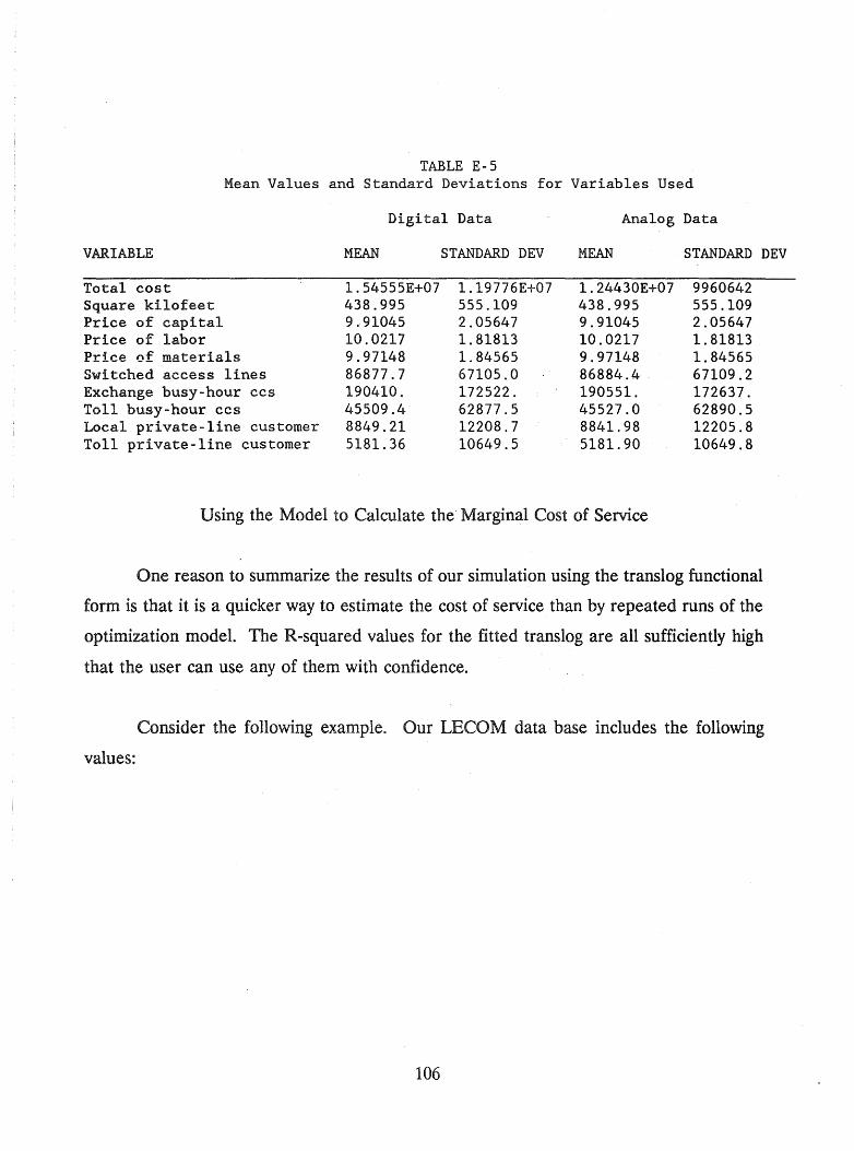
TABLE E-5 Mean Values and Standard Deviations for Variables Used
Digital Data Analog Data
VARIABLE MEAN STANDARD DEV MEAN STANDARD DEV
Total cost 1.54555E+07 1.19776E+07 1. 24430E+07 9960642 Square ki10feet 438.995 555.109 438.995 555.109 Price of capital 9.91045 2.05647 9.91045 2.05647 Price of labor 10.0217 1.81813 10.0217 1.81813 Price of materials 9.97148 1.84565 9.97148 1.84565 Switched access lines 86877.7 67105.0 86884.4 67109.2 Exchange busy-hour ccs 190410. 172522. 190551. 172637. Toll busy-hour ccs 45509.4 62877.5 45527.0 62890.5 Local private-line customer 8849.21 12208.7 8841.98 12205.8 Toll private-line customer 5181.36 10649.5 5181.90 10649.8
Using the Model to Calculate the Marginal Cost of Service
One reason to summarize the results of our simulation using the translog functional
form is that it is a quicker way to estimate the cost of service than by repeated runs of the
optimization model. The R-squared values for the fitted translog are all sufficiently high
that the user can use any of them with confidence.
Consider the following example. Our LECO M data base includes the following
values:
106
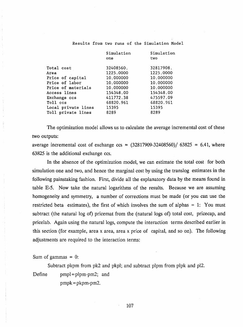
Results from two runs of the Simulation Model
Simulation Simulation one two
Total cost 32408560. 32817908. Area 1225.0000 1225.0000 Price of capital 10.000000 10.000000 Price of labor 10.000000 10.000000 Price of materials 10.000000 10.000000 Access lines 154348.00 154348.00 Exchange ccs 411772.38 475597.09 Toll ccs hSHP)(\ Qh 1
vVU&.V.JV.I.. 68820.961 Local private lines 15395 15395 Toll private lines 8289 8289
The optimization model allows us to calculate the average incremental cost of these
two outputs:
average incremental cost of exchange ccs = (32817909-32408560)/ 63825 = 6.41, where
63825 is the additional exchange ccs.
In the absence of the optimization model, we can estimate the total cost for both
simulation one and two, and hence the marginal cost by using the translog estimates in the
following painstaking fashion. First, divide all the explanatory data by the means found in
table E-5. Now take the natural logarithms of the results. Because we are assuming
homogeneity and symmetry, a number of corrections must be made (or you can use the
restricted beta estimates), the first of which involves the sum of alphas = 1: You must
subtract (the natural log of) pricemat from the (natural logs of) total cost, pricecap, and
pricelab. Again using the natural logs, compute the interaction terms described earlier in
this section (for example, area x area, area x price of capital, and so on). The following
adjustments are required to the interaction terms:
Sum of gammas = 0:
Subtract pkpm from pk2 and pkpl; and subtract plpm from plpk and p12.
Define pmpl=plpm-pm2; and
pmpk = pkpm-pm2.
107

Symmetry restrictions:
Add plpk to pkpl; pmpk to pkpm; and pmpl to plpm.
Sum of rhos = 0:
Subtract pmexccs from pkexccs and plexccs; subtract pmtlccs from pktlccs and pltlccs;
subtract pmlpl from pklpl and pllpl; and, finally, subtract pmtpl from pktpl and pltpl.
The following is a summary of these computations.
Using the Translog Parameters to Estimate the Cost of Service
const area pricecap pricelab acclines exchccs tlccsec lcplcust tlplcust ar2 arpk arpl arpm aral arexccs artlccs arlpl artpl pk2 pkpl pkpm pkal pkexccs pktlccs pklpl pktpl p12 plpm pIal
Simulation one 1.00000 1.02621 0.00613900 -0.00501977 0.574709 0.771289 0.413589 0.553689 0.469911 1.05310 0.00923057 -0.00222065 0.00293068 0.589770 0.791502 0.424428 0.568200 0.482226 5.52194E-05 -5.84364E-05 4.32198E-05 0.00352814 0.00473494 0.00253903 0.00339910 0.00288478 1.08624E-05 -2.05155E-05 -0.00288490
108
Simulation two
1.00000 1.02621 0.00613900 -0.00501977 0.574709 0.915389 0.413589 0.553689 0.469911 1.05310 0.00923057 -0.00222065 0.00293068 0.589770 0.939379 0.424428 0.568200 0.482226 5.52194E-05 -5.84364E-05 4.32198E-05 0.00352814 0.00561958 0.00253903 0.00339910 0.00288478 1.08624E-05 .. 2.05155E-05 -0.00288490
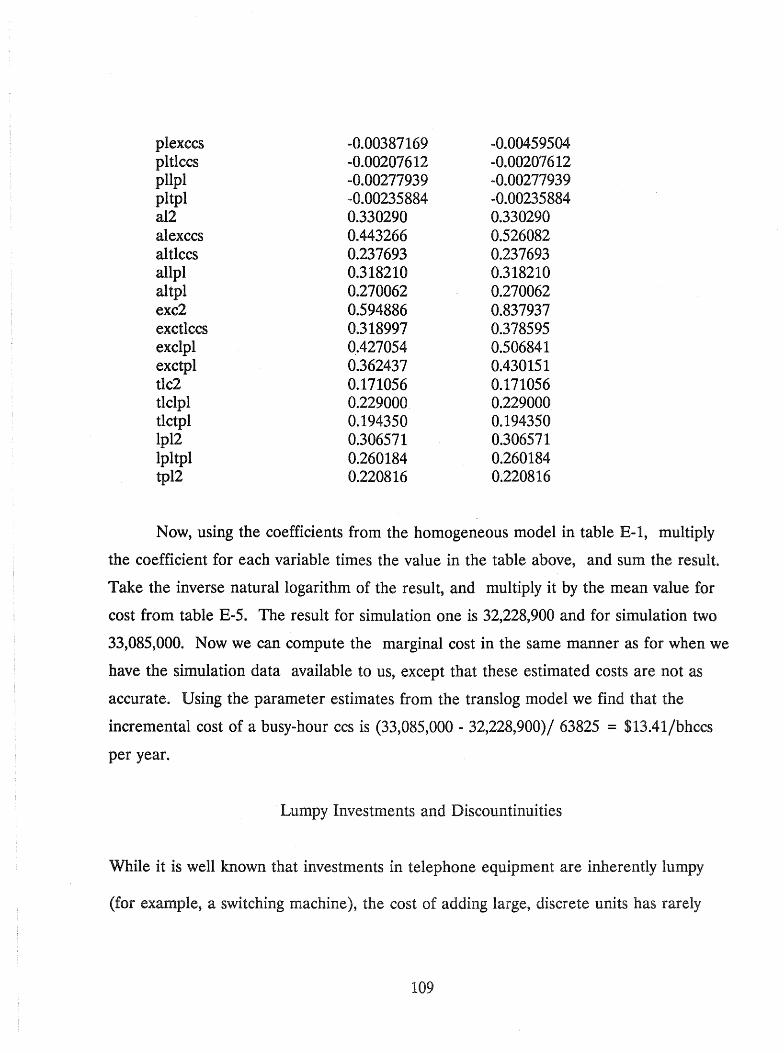
plexccs -0.00387169 -0.00459504 pltlccs -0.00207612 -0.00207612 pllpl -0.00277939 -0.00277939 pltpl -0.00235884 ·0.00235884 al2 0.330290 0.330290 alexccs 0.443266 0.526082 altlccs 0.237693 0.237693 allpl 0.318210 0.318210 altpl 0.270062 0.270062 exc2 0.594886 0.837937 exctlccs 0.318997 0.378595 exclpl 0.427054 0.506841 exctpl 0.362437 0.430151 tlc2 0.171056 0.171056 tlclpl 0.229000 0.229000 tlctpl 0.194350 0.194350 Ipl2 0.306571 0.306571 lpltpl 0.260184 0.260184 tpl2 0.220816 0.220816
Now, using the coefficients from the homogeneous model in table E-1, multiply
the coefficient for each variable times the value in the table above, and sum the result.
Take the inverse natural logarithm of the result, and multiply it by the mean value for
cost from table E-5. The result for simulation one is 32,228,900 and for simulation two
33,085,000. Now we can compute the marginal cost in the same manner as for when we
have the simulation data available to us, except that these estimated costs are not as
accurate. Using the parameter estimates from the translog model we find that the
incremental cost of a busy-hour ccs is (33,085,000 - 32,228,900)/ 63825 = $13.41/bhccs
per year.
Lumpy Investments and Discountinuities
While it is well known that investments in telephone equipment are inherently lumpy
(for example, a switching machine), the cost of adding large, discrete units has rarely
109
been discussed. This section illustrates the source of the cost lumps and explains how
they affect the cost of providing service.
The switching equipment in a central office is placed on frames, which have
varying degrees of line and usage capacity. Once a frame is installed, the marginal cost
of using the facility is small. But if the capacity of the frame is exhausted, a new, costly
frame must be ir.t.Stalled.
For example, in a large digital switch (for example, DMS10Q®), customers lines
are terminated on line modules. A line module can terminate approximately 1,200 lines.
The volume of busy-hour traffic per customer determines the number of network frames
required for making connections between line modules or connecting customers to
interoffice trunks.
If the busy-hour usage per customer is 3.00 ccs, two network frames may be
needed to serve five line modules.3 If busy-hour ccs usage increases to 3.10, two
network frames still would satisfy customers' peak usage requirements. But if the busy
hour increases beyond a critical point, assumed to be 3.20 bhccs, an additional network
frame will be required. The addition of a third network frame leads to 'a significant
increase in the cost of service. The cost impact of this lumpy investment is illustrated in
Table XXIII. For a city with approximately 37,000 customers, we estimated the average
incremental cost of an increase in 2,100 toll busy-hour ccs. The incremental cost, per
busy-hour ccs is reported below.4
~e equipment engineering numbers used in this example are hypothetical.
~e data include the cost of interoffice transport and toll tandem switching.
110
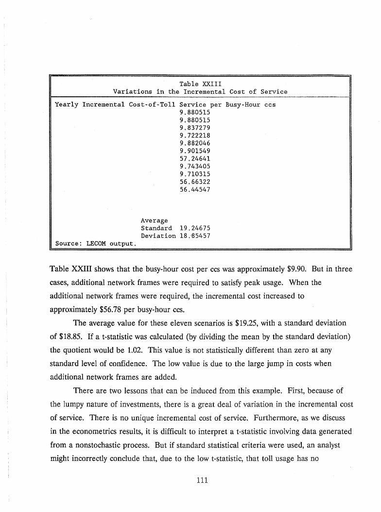
Table XXIII Variations in the Incremental Cost of Service
Yearly Incremental Cost-of-Toll Service per Busy-Hour ccs 9.880515
Source: LECOM output.
9.880515 9.837279 9.722218 9.882046 9.901549 57.24641 9.743405 9.710315 56.66322 56.44547
Average Standard 19.24675 Deviation 18.~5457
Table XXIII shows that the busy-hour cost per ccs was approximately $9.90. But in three
cases, additional network frames were required to satisfy peak usage. When the
additional network frames were required, the· incremental cost increased to
approximately $56.78 per busy-hour ccs.
The average value for these eleven scenarios is $19.25, with a standard deviation
of $18.85. If a t-statistic was calculated (by dividing the mean by the standard deviation)
the quotient would be 1.02. This value is not statistically different than zero at any
standard level of confidence. The low value is due to the large jump in costs when
additional network frames are added.
There are two lessons that can be induced from this example. First, because of
the lumpy nature of investments, there is a great deal of variation in the incremental cost
of service. There is no unique incremental cost of service. Furthermore, as we discuss
in the econometrics results, it is difficult to interpret a t-statistic involving data generated
from a nonstochastic process. But if standard statistical criteria were used, an analyst
might incorrectly conclude that, due to the low t-statistic, that toll usage has no
111

statistically significant affect on the cost of service. This would be an incorrect
conclusion--the low t-statistic would merely reflect the large variation in the incremental
cost of service.5
5The discontinuity can not be easily taken into account by adding dummy variables-there are too many discontinues in the cable, switching and trunking engineering algorithms.
112
I. INTRODUCTION
APPENDIX TWO
LECOM MANU,AL
This manual describes the structure and operation of LECOM (Local Exchange Cost
Optimization Model). This software has been developed by D. Mark Kennet of Tulane
University and David J. Gabel of Queens College, partially funded by a contract with
The ~1ational Regulatory Research Institute. The PC version of the prograrns were
developed and compiled in Turbo Pascal, a product of Borland International, Inc.
A What do the programs do?
The programs take as input demographic data for a city, price data on the technological
options available, and usage data for the three types of consumers to optimally site
switching facilities on a stylized map of the city.
B. How do the programs work?
The programs compute the annualized cost of service for a given switch
location/technology configuration and adjust the location using a derivative-free
algorithm until the cost of service is at its minimum value. An exhaustive search over
technological configurations is performed, with the location optimization performed for
each one until the cost-minimizing technology and location are identified.
c. What are the programs good for?
The programs have a number of uses. The authors are currently involved in a study
which estimates an economic cost function using program output simulated repeatedly;
other similar uses can be anticipated. Other uses are long-range planning for utility
executives, assessment of long-run marginal costs of service for utility regulators, and
information for rate-case intervenors.
113

D. What do I need to run the programs?
An MS-DOS based PC with 8086,80286, or 80386 processor,
640 K of RAM,
Math coprocessor (optional but very helpful),
Hard disk (also optional),
Accurate data,
Time and patience (especially if you have a machine running at a relatively low clock
speed).
E. What are the limitations of the programs?
The programs can locate up to thirty central offices with the PC
version, serving up to 300 serving areas. This is equivalent to a city size of
approximately 180,000 customers (assuming 600 customers per serving area).
Contact the authors of this report regarding use of the program for larger cities.
F. Where can I go for help if I need it?
Support for the programs is provided by the authors.
Mark Kennet
Tulane University
Department of Economics
New Orleans, LA 70017
504-865-5321
David Gabel
Queens College
Department of Economics
Flushing, NY 11367
718-997-5452
We recommend that frequent users of the program mail David Gabel their name and
address. We will send them a notice regarding any subsequent changes to the program.
114
II. GETIING STARTED
A Hard disk systems
1. Create a subdirectory for the software; for example, TELEPHON. Do
this by first making sure that you are in the root directory of your
hard disk (that is, observe that the DOS prompt is 'C:\'. If the prompt is 'C>', you need
to type the command
prompt $p$g < Enter>
to have DOS tell you which subdirectory you are in). To get to the root directory, type
the command
cd \ <Enter>
which takes you to the root. N ow create the subdirectory TELEPHON by
entering
md telephon < Enter> .
2. Create two subdirectories within TELEPHON: DIGITAL and ANALOG. You can
do this by typing
cd \ telephon < Enter>
and then
md digital <Enter>
md analog < Enter> .
115
3. Copy the analog programs:
copy a: \analog\ *. * c: \ telephon \analog\ *. * < Enter>
4. Copy the digital programs:
copy a:\digital\ *.* c:\telephon\digital\ *.* <Enter>
You are now ready to use the programs.
B. Floppy-disk only systems
The programs are ready to run if your system is a floppy-disk only machine. However,
you may wish to make a backup of the diskette containing the software before you use it.
Simply make a backup copy of your software on another formatted empty disk. To learn
how to format a disk, see your DOS manual. To accomplish the copying, put the
original diskette in Drive A, and the new formatted diskette in Drive B, if you have a
Drive B.
N ow if your computer has two floppy drives, type
xcopy a: b: / s < Enter>
or, if your machine has one floppy drive, type
xcopy a: a: / s < Enter>
and follow any directions your computer gives you (this last statement is relevant to
owners of one-floppy systems). Mter you complete these tasks, put the original diskette
in a safe place and put the new copy in floppy Drive A
116
III. EDITING DATA FILES
There are three data files required by each of the digital and
analog programs. Two of these files can be the same for both analog and digital
computations; however, the third is specific to the technology being examined. For the
analog programs, the files required are POPULATN.DAT,
RECfANGL.DAT, GAUGEDST.DAT, and VARIABLE.DAT. POPULATN.DAT is a
file containing map information for the city of interest, projected number of customers in
each serving area, and the number of customers in each classification: business, medium
density, and residential. RECfANGL.DAT is a file that can either be created by the
user or automatically using the program CITYINIT.EXE. RECfANGL.DAT contains
the number of serving areas in the city, and data arranged serving area by serving area
on the number of customers, the type of customer, and coordinates of the northeast and
southwest corners of the serving area (setting the origin equal to the southwest corner of
the city). It is recommended that new users NOT attempt to change RECfANGL.DAT
but instead allow the CITYINIT.EXE program to make any changes.
GAUGEDST.DAT contains data on the recommended mix of gauges for various
lengths of cables; it can be modified by using any text editor, but it is also recommended
that new users not alter this file. Finally, V ARIABLE.DAT contains the price, usage,
and capacity data as well as data required by the program for technical reasons.
The first four digital data files are identical to the analog files. The corresponding file to
VARIABLE.DAT is called DVARIABL.DAT. The digital program requires one other
file, DXOVER.DAT. This file is created by the program DXINIT.DAT; once again, the
user is free to modify this text file containing two numbers, but we strongly recommend
against doing so.
To edit any of the files, simply use your favorite text editor.
The files come complete with "comments" embedded within so that you can see what
each variable is and what its definition is. The program's input is format-free, so that
you don't have to worry about lining up any numbers; however, there must always be a
space or a carriage return between any two numbers in the data file. The data files
MUST BE SAYED AS ASCII TEXT FILES.
117
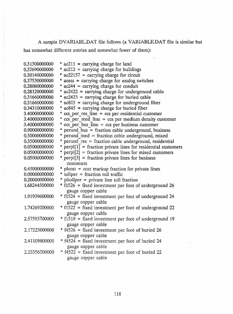
A sample DVARIABL.DAT file follows (a VARIABLE.DAT file is similar but
has somewhat different entries and somewhat fewer of them):
0.31300000000 0.32690000000 0.30140000000 0.37530000000 0.28080000000 0.28120000000 0.31660000000 0.31660000000 0.34310000000 3.40000000000 3.40000000000 3.40000000000 0.90000000000 0.50000000000 0.35000000000 0.05000000000 0.05000000000 0.05000000000
0.45000000000 0.00000000000 0.20000000000 1.68244500000
1.91939600000
1.74269200000
2.57593700000
2.17225000000
2.41109800000
2.23356200000
* ac211 = carrying charge for land * ac212 = carrying charge for buildings * ac22157 = carrying charge for circuit * acess = carrying charge for analog switches * ac244 = carrying charge for conduit * ac2422 = carrying charge for underground cable * ac2423 = carrying charge for buried cable * ac815 = carrying charge for underground fiber * ac845 = carrying charge for buried fiber * ccs yer _res_line = ccs per residential customer * ccs yer _ med _line = ccs per medium density customer * ccs yer _ bus _line = ccs per business customer * perund _ bus = fraction cable underground, business * perund _ med = fraction cable underground, mixed * perund res = fraction cable underground, residential * perpl[1] = fraction private lines for residential customers * perpl[2] = fraction private lines for mixed customers * perpl[3] = fraction private lines for business
customers * plcost = cost markup fraction for private lines * toUper . = fraction toll traffic * pltollper = private line toll fraction * f1526 = fixed investment per foot of underground 26
gauge copper cable * f1524 = fixed investment per foot of underground 24
gauge copper cable * f1522 = fixed investment per foot of underground 22
gauge copper cable * f1519 = fixed investment per foot of underground 19
gauge copper cable * f4526 = fixed investment per foot of buried 26
gauge copper cable * f4524 = fixed investment per foot of buried 24
gauge copper cable * f4522 = fixed investment per foot of buried 22
gauge copper cable
118
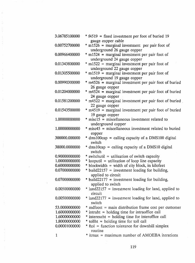
3.06785100000
0.00752700000
0.00966400000
0.01343800000
0.01305500000
0.00990300000
0.01204000000
0.01581200000
0.01543500000
1.00000000000
1.00000000000
300000.000000
38000.0000000
0.90000000000 1.00000000000 0.60000000000 0.07000000000
0.07000000000
0.00500000000
0.00500000000
53.0000000000 1.60000000000 1.60000000000 1.80000000000 0.00001000000
1
* f4519 = fixed investment per foot of buried 19 gauge copper cable
* m1526 = marginal investment per pair foot of underground 26 gauge copper
* m1524 = marginal investment per pair foot of underground 24 gauge copper
* m1522 = marginal investment per pair foot of underground 22 gauge copper
* m1519 = marginal investment per pair foot of underground 19 gauge copper
* m4,\"h: - TnartT;nt:ll In'Iu::>cotTnant nar na;r fAAt Af hHP;"",r1 .L.A. - .J4.#V = .1..I • ..l .l.6..l.l..l.u.I. .1..1. ... "".,I..I...l.l."".I..l.1. P"".I. P ..l.l. .LVVI. V.L U'U.l..I.\,;-u
26 gauge copper * m4524 = marginal investment per pair foot of buried
24 gauge copper * m4522 = marginal investment per pair foot of buried ,
22 gauge copper * m4519 = marginal investment per pair foot of buried
19 gauge copper * mise 15 = miscellaneous investment related to
underground copper * misc45 = miscellaneous investment related to buried
copper * dmslOOcap = calling capacity of a DMS100 digital
switch * dms10cap = calling capacity of a DMS10 digital
switch * switchutil = utilization of switch capacity * looputil = utilization of loop line capacity * blockwidth = width of city block, in kilofeet * build22157 = investment loading for building,
applied to circuit * build22177 = investment loading for building,
applied to switch * land22157 = investment loading for land, applied to
circuit * land22177 = investment loading for land, applied to
switch * mdfcost = main distribution frame cost per customer * intraht = holding time for intraoffice call * interexcht = holding time for interoffice call * tollht = holding time for toll call * ftol = function tolerance for downhill simplex
routine * itmax = maximum number of AMOEBA iterations
119
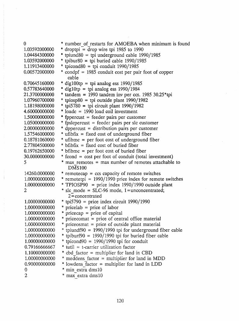
o 1.03592000000 1.04484300000 1.03592000000 1.11913400000 0.00572000000
0.70645160000 0.57783640000 21.3700000000 1.07960700000 1.18198000000 4.60000000000 1.50000000000 1.05000000000 2.00000000000 1.57546000000 0.18781060000 2.77804500000 0.19762650000 30.0000000000 5
14260.0000000 1.00000000000 1.00000000000 2
1.00000000000 1.00000000000 1.00000000000 1.00000000000 1.00000000000 1.00000000000 1.00000000000 1.00000000000 0.79166666667 1.10000000000 1.00000000000 0.90000000000 o 2
* number of restarts for AMOEBA when minimum is found * droptpi = drop wire tpi 1985 to 1990 * tpiund80 = tpi underground cable 1990/1985 * tpibur80 = tpi buried cable 1990/1985 * tpicond80 = tpi conduit 1990/1985 * condpf = 1985 conduit cost per pair foot of copper
cable * dig100tp = tpi analog ess 1990/1985 * dig10tp = tpi analog ess 1990/1984 * tandem = 1990 tandem inv per ccs. 1985 30.25*tpi * tninc::.nRO = tnl nnts1ttp nl~nt 1000/1 OR? "YJL""UY,",'V "Y.IL "'''''''' &"-6"" t'.a.~.&. ... "" '&'''''''''''1 ..... ,.,...,..,
* tpi5780 = tpi circuit plant 1990/1982 * loadc = 1990 load coil investment * fppercust = feeder pairs per customer * fpslcpercust = feeder pairs per sIc customer * dppercust = distribution pairs per customer * ufibfix = fixed cost of underground fiber * ufibmc = per foot cost of underground fiber * bfibfix = fixed cost of buried fiber * bfibmc = per foot cost of buried fiber * fcond = cost per foot of conduit (total investment) * max remotes = max number of remotes attachable to
DMS100 * remotecap = ccs capacity of remote switches * remotetpi = 1990/1990 price index for remote switches * TPIOSP90 = price index 1990/1990 outside plant * sIc_mode = SLC-96 mode, 1 = unconcentrated;
2 = concentrated lie tpi5790 = price index circuit 1990/1990 * pricelab = price oJ labor * pricecap = price of capital * pricecomat = price of central office material * priceosmat = price of outside plant material * tpiundf90 = 1990/1990 tpi for underground fiber cable lie tpiburf90 = 1990/1990 tpi for buried fiber cable * tpicond90 = 1990/1990 tpi for conduit lit tutH = t-carrier utilization factor * cbd factor = multiplier for land in CBD lit meddens factor = multiplier for land in MDD * lowdens factor = multiplier for land in LDD * min extra dms10 lit max extra dms 10

See the data requirements appendix (page 145) for the precise definitions of these
variables.
Among the variables over which the user has control in this file are three which
pertain to the nonlinear optimization routine used to optimize the locations of the
switches. These are ftol, itmax, and number _of_restarts. The first, ftol, is simply the
convergence value for the routine: when the optimization routine finds what it "thinks" is
the cost minimizing location, it will check to make sure that it cannot improve the
solution by more than this amount. You should not make this number smaller than le-6
or so; few computers can improve on this level of precision. The variable itmax is the
maximum number of iterations the optimization routine will try before concluding that it
cannot locate the cost minimizing location. Five hundred is a reasonable number to use;
however, some users may find, particularly with larger cities, that a larger number is
desirable, while others may find that reducing this number is a way of speeding up the
program when an exact solution is not important.
The user-defined number _of_restarts is the number of times the program will
attempt to reoptimize once a solution is found. Reoptimizing is necessary because of the
nonconcave nature of the objective function being minimized: It is theoretically possible
that any given location solution is only a local, rather than a global, minimizer. We
recommend a value of 1 to 4 for this number, although any nonnegative integer will
work.
IV. OPERATING THE PROGRAMS
Once you have edited the data files and you feel sure that you have set up the
data in the way you would like, you are ready to run the modules. In the case of the
analog programs, there are two programs you must run in sequence; in the case of digital
programs, three.
121

A. Analog program operation
If you are running the modules for the first time or if you have changed any of
the data in POPULATN.DAT, you must run the program CITYINIT.EXE (unless you
wish to create and edit the file RECfANGL.DAT manually; see the data requirements
appendix for instructions on how to do this. After the file RECTANGL.DAT has been
created either by CITYINIT.EXE or by hand, you can run ANALOG.EXE. Step by step
instructions follow.
1. This step is necessary the first time you run the program and EVERY TIME
YOU CHANGE THE FILE POPULATN.DAT. If this does not apply to you, go to step
2. Type the command
cd\telephon\analog <Enter>
and make sure that the files POPULATN.DAT, VARIABLE. D AT, and
GAUGEDST.DAT are in the directory by typing
dir * .dat < Enter>
which will result in your screen presenting the names of these files if they are present. If
the files are there, type
cityinit < Enter>
and continue to step 2.
122
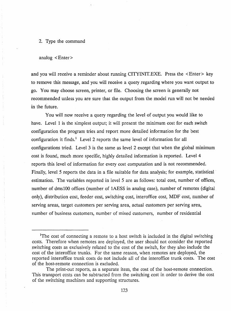
2. Type the command
analog < Enter>
and you will receive a reminder about running CITYINIT.EXE. Press the < Enter> key
to remove this message, and you will receive a query regarding where you want output to
go. You may choose screen, printer, or file. Choosing the screen is generally not
rccoITllucnded unless you are sure that the output from the model run will not be needed
in the future.
You will now receive a query regarding the level of output you would like to
have. Level 1 is the simplest output; it will present the minimum cost for each switch
configuration the program tries and report more detailed information for the best
configuration it finds. I Level 2 reports the same level of information for all
configurations tried. Level 3 is the same as level 2 except that when the global minimum
cost is found, much more specific, highly detailed information is reported. Level 4
reports this level of information for every cost computation and is not recommended.
Finally, level 5 reports the data in a file suitable for data analysis; for example, statistical '
estimation. The variables reported in level 5 are as follows: total cost, number of offices,
number of dms100 offices (number of 1AESS in analog case), number of remotes (digital
only), distribution cost, feeder cost, switching cost, interoffice cost, MDF cost, number of
serving areas, target customers per serving area, actual customers per serving area,
number of business customers, number of mixed customers, number of residential
IThe cost of connecting a remote to a host switch is included in the digital switching costs. Therefore when remotes are deployed, the user should not consider the reported switching costs as exclusively related to the cost of the switch, for they also include the cost of the interoffice trunks. For the same reason, when remotes are deployed, the reported interoffice trunk costs do not include all of the interoffice trunk costs. The cost o(the host-remote connection is excluded.
The print-out reports, as a separate item, the cost of the host-remote connection. This transport costs can be subtracted from the switching cost in order to derive the cost of the switching machines and supporting structures.
123
customers, number of private line customers, private line cost markup, private line toll
percentage, business private line percentage, mixed private line percentage, residential
private line percentage, intraoffice message volume, exchange interoffice message
volume, toll message volume, intraoffice ccs, exchange interoffice ccs, toll ccs, toll
percentage, business ccs per line, mixed ccs per line, residential ccs per line, loop
length2, length of slc-96 (digital only); price of labor (index), price of capital (index),
price of central office materials (index), price of outside plant materials (index), central
business district coordinates (upper right, lower left), medium density district coordinates
(upper right, lower left), city upper right coordinates, locations of switches.
Note that the program may run for quite some time--sometimes as
long as several days.
B. Digital program operation
If you are running the modules for the first time or if you have changed any of
the data in POPULATN.DAT, you must run the program CITYINIT.EXE (unless you
wish to create and edit the file RECTANGL.DAT manually; see the data requirements
appendix for instructions on how to do this. After the file RECTANGL.DAT has been
created either by CITYINIT.EXE or by hand, you can run DIGITAL.EXE. Step by step
instructions follow.
1. This step is necessary the first time you run the program and EVERY TIME
YOU CHANGE THE FILE POPULATN.DAT. If this does not apply to you, go to step
2In order to determine the loop length per customer, divide the loop length by the number of serving areas. The quotient is the kilofoot loop length per customer. The same procedure should be used for the slc-96 length (the next variable in the digital model). For both items in the file, they are calculated by summing the average loop length of reaching one customer in each I.;:erving area.
124
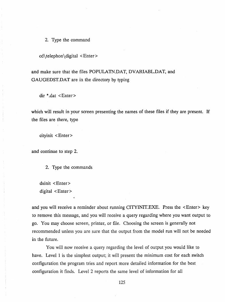
2. Type the command
cd\ telephon \ digital < Enter>
and make sure that the files POPULATN.DAT, DVARIABL.DAT, and
GAUGEDST.DAT are in the directory by typing
dir * .dat < Enter>
which will result in your screen presenting the names of these files if they are present. If
the files are there, type
cityinit < Enter>
and continue to step 2.
2. Type the commands
dxinit < Enter>
digital < Enter>
and you will receive a reminder about running CITYINIT.EXE. Press the < Enter> key
to remove this message, and you will receive a query regarding where you want output to
go. You may choose screen, printer, or file. Choosing the screen is generally not
recommended unless you are sure that the output from the model run will not be needed
in the future.
You will now receive a query regarding the level of output you would like to
have. Level 1 is the simplest output; it will present the minimum cost for each switch
configuration the program tries and report more detailed information for the best
configuration it finds. Level 2 reports the same level of information for all
125
configurations tried. Level 3 is the same as level 2 except that when the global minimum
cost is found, much more specific, highly detailed information is reported. Level 4
reports this level of information for every cost computation and is not recommended.
Finally, level 5 reports the data in a file suitable for data analysis; for example, statistical
estimation.
Note that, as in the analog case, the program may run for quite some
time--sometimes as long as several days.
v. Spreadsheets for Generating Data Files and Analyzing Results
Creating Files for the Model
In our computer study of the cost function we analyzed the effect of increasing the
demand of one service while holding all other variables constant. By holding all but one
variable constant, we constructed what are known as orthogonal data. There are a few
advantages to constructing orthogonal data. First, the average incremental cost of a
service can be determined without doing any regression analysis (the incremental cost is
divided by the incremental usage of the one service whose demand has not been held
constant).
Second, when undertaking regression analysis, the construction of an orthogonal
data set reduces the collinearity in the data. This makes its easier to invert the matrix of
independent variables, and reduces the standard deviation of the estimated coefficients.
Finally, because of the orthogonal nature of the data, it isa straightforward
project to test the reasonableness of the results. We use the following procedure to test
the reasonableness of the results.
We assume there are five services.
X( 1) = exchange ccs
X(2) = toll ccs
X(3) = local private line
X(4) = toll private line
126

X(5) = switched access lines3
On the enclosed computer disk you will find Lotus spreadsheets that can be used
to create the files. Subdirectory LOTUS22 contains file "nrriexam.wk1.,t4 In order to
create files, the user should make entries in the cells identified in the following chart.
3We use the term "service" loosely. More precisely, we study the impact on cost of four services, and the joint input switched access.
~is worksheet is for illustrative purposes only. For actual study work, the user should use the other spreadsheets in the subdirectory. NRRIEXAM.WK1 has been modified so that the model provides cost estimates without conducting an exhaustive location search. This was done by setting the number of iterations to one and the number of restarts to zero.
127

Creating Files
CELL DEFINITION
C10 CUSTOMERS IN BUSINESS DISTRICT (BOTH PRIVATE LINE AND SWITCHED)
Cll CUSTOMERS IN MIXED BUSINESS/ RESIDENTIAL DISTRICT
C12 CUSTOMERS IN RESIDENTIAL DISTRICT
D10 PERCENT OF CUSTOMERS IN BUSINESS DISTRICT WHOM ARE PRIVATE LINE CUSTOMERS
Dll PERCENT OF CUSTOMERS IN MIXED DISTRICT WHOM ARE PRIVATE LINE CUSTOMERS
D12 PERCENT OF CUSTOMERS IN RESIDENTIAL DISTRICT WHOM ARE PRIVATE LINE CUSTOMERS
E10 = Ell .... El2 PERCENT OF PRIVATE LINES WHICH ARE TOLL PRIVATE LINE (USE SAME VALUE FOR ALL THREE CELLS)
J10 CCS BUSY-HOUR USAGE PER SWITCHED BUSINESS SUBSCRIBER
Jll CCS BUSY-HOUR USAGE PER SWITCHED MIXED SUBSCRIBER f-'-
Jl2 CCS BUSY-HOUR USAGE PER SWITCHED RESIDENTIAL SUBSCRIBER
Fl4 STIMULATION FACTOR (DETERMINES THE AMOUNT BY WHICH USAGE WILL BE INCREASED. A VALUE OF 1.05 HERE WOULD INCREASE USAGE BY FIVE PERCENT)
Working with file NRRIEXAM. WK1, we can see how to estimate the marginal
cost of different services.
The worksheet has been used to export file numbers variable.452 through
variable.468, as well as populatn.166 through populatn.172 (these files appear,
respectively, in subdirectories V ARFILES and POPULA TN).
128

The steps for exporting files are identified below.
1. The variable files were exported by first going to cell C157. In cell ClS7 an
arbitrary number was placed for identifying the different variable files that were created.
In cell C1484 a number was placed to initiate the number of the population files.
Movement is expedited by using the F5 function key.
2. Push F9 (the calculate putton for LOTUS).
3. move to Cell a157. You will see the following:
I A I I al I c I I 0 I I E I I I I I I I I I 157 variable 452 233 158 0.31300000000 '* ac211 159 0.32680000000 '* ac212 160 0.29860000000 '* ac22157 161 0.28680000000 '* acess 162 0.28080000000 '* ac244 163 0.28120000000 '* ac2422 164 0.31660000000 '* ac2423
4. Use the cursor key to move down to cell A158.
5. Note the entry in cell D 157. This tells us the end of the range that we want to
export for our first variable file. In this example, the number is 233.
6. Execute the following LOTUS commands:
a. /P F (PRINT A FILE)
b. variable.452 (this is the name of the file. We always use the prefix
variable, and the identifying number for our first file appears in cell C157.
c. /0 d.M
E.R F.100
G.M
H.T
1.0
1.M
(SELECT OPTIONS)
(MARGINS OPTION)
(MODIFY RIGHT HAND MARGIN)
(SET RIGHT-HAND MARGIN EQUAL TO 100)
(MODIFY TOP MARGIN)
(T FOR TOP)
(0 TOP MARGIN)
(B MODIFY TOP MARGIN)
129
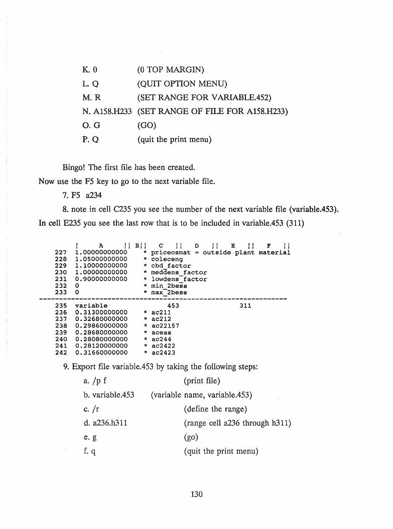
K.O
L.Q
M.R
N. A158.H233
O.G
P. Q
(0 TOP MARGIN)
(QUIT OPTION MENU)
(SET RANGE FOR V ARIABLE.452)
(SET RANGE OF FILE FOR A158.H233)
(GO)
(quit the print menu)
Bingo! The first file has been created.
N ow use the F5 key to go to the next variable file.
7. F5 a234
8. note in cell C235 you see the number of the next variable file (variable.453).
In cell E235 you see the last row that is to be included in variable.453 (311)
227 228 229 230 231 232 233
235 236 237 238 239 240 241 242
I A II 1.00000000000 1.05000000000 1.10000000000 1.00000000000 0.90000000000 o o
variable 0.31300000000 0.32680000000 0.29860000000 0.28680000000 0.28080000000 0.28120000000 0.31660000000
BII c II D II E II F II * priceosmat = outside plant material * coleceng * cbd factor * meddens factor * lowdens-factor * min 2bess * max-2bess
453 * ac211 '* ac212 '* ac22157 '* acess '* ac244 * ac2422 * ac2423
311
9. Export file variable.453 by taking the following steps:
a. Ip f (print file)
b. variable.453
c·/r d. a236.h311
e.g
f. q
(variable name, variable.453)
(define the range)
(range cell a236 through h311)
(go)
(quit the print menu)
130
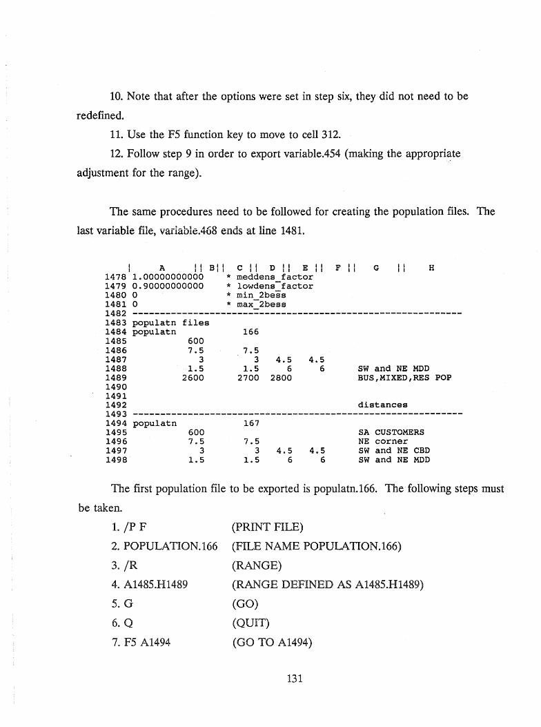
10. Note that after the options were set in step six, they did not need to be
redefined.
11. Use the F5 function key to move to cell 312.
12. Follow step 9 in order to export variable.454 (making the appropri~te
adjustment for the range).
The same procedures need to be followed for creating the population files. The
last variable file, variable.468 ends at line 1481.
I A II BII C II D II E II F II G II H 1478 1.00000000000 * meddens factor 1479 0.90000000000 * lowdens-factor 1480 0 * min 2bess 1481 0 * max-2bess 1482 ------------------------------------------------------------1483 populatn 1484 populatn 1485 1486 1487 1488 1489 1490 1491 1492
files
600 7.5
3 1.5
2600
166
7.5 3 4.5
105 6 2700 2800
405 6 SW and NE MDD
BUS,MIXED,RES POP
distances 1493 ------------------------------------------------------------1494 populatn 1495 1496 1497 1498
600 7.5
3 1.5
167
7.5 3
1.5 4.5
6 4.5
6
SA CUSTOMERS NE corner sw and NE CBD sw and NE MDD
The first population file to be exported is populatn.166. The following steps must
be taken.
1. IP F
2. POPULATION.166
3·/R
4. A1485.H1489
5. G
6. Q
7. F5 A1494
(PRINT FILE)
(FILE NAME POPULATION.166)
(RANGE)
(RANGE DEFINED AS A1485.H1489)
(GO)
(QUIT)
(GO TO A1494)
131

8. IP F (PRINT FILE)
9. POPULATION.167
10·/R
(FILE NAME POPULATION.167)
(RANGE)
11. A1495.H1499 (RANGE DEFINED AS A1495.H1499)
(GO) 12. G
13. Q (QUIT)
14. Follow the same steps to create population.168 through 172.
In order to verify that you have correctly exported the files, you may compare
your files with the files that appear in subdirectories varfiles and population.
Running the Files
Running the program is a simple matter and is described at page 121. For the
files just created, the appropriate combination of files are identified at the bottom of
NRRIEXAM.WK1
(cells A1557 through C1573)
I A 1556 populatn 1557 1558 1559 1560 1561 1562 1563 1564 1565 1566 1567 1568 1569 1570 1571 1572 1573
II BII c I variable
166 452 166 453 166 454 167 455 168 456 166 457 170 458 169 459 171 460 167 461 168 462 170 463 167 464 168 465 170 466 172 467 166 468
To run the first combination of files (populatn.166 and variable.452), do the
following steps (at the DOS prompt):
132
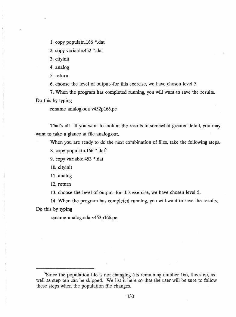
1. copy populatn.166 * .dat
2. copy variable.452 * .dat
3. cityinit
4. analog
5. return
6. choose the level of output--for this exercise, we have chosen level 5.
7. When the program has completed running, you will want· to save the results.
Do this by typing
rename analog.oda v452p 166.pc
That's all. If you want to look at the results in somewhat greater detail, you may
want to take a glance at file analog. out.
When you are ready to do the next combination of files, take the following steps.
8. copy populatn.166 * .datS
9. copy variable.453 * .dat
10. cityinit
11. analog
12. return
13. choose the level of output--for this exercise, we have chosen level 5.
14. When the program has completed running, you will want to save the results.
Do this by typing
rename analog.oda v453p 166.pc
SSince the population file is not changing (its remaining number 166, this step, as well as step ten can be skipped. We list it here so that the user will be sure to follow these steps when the population file changes.
133

Output Evaluation
You can compare your results with the results that appear in subdirectory
ANALRESU.
We have also provided you with a LOTUS spreadsheet that aids in the calculation
of the incremental cost of service (ANALEXAM.WK1). The files that have just been
created should be loaded on to the worksheet. In row one of ANALEXAM, we identify
the variable name.
The following steps are followed.
1. Go to cell A2
2. IF I N (import number file)
3. V452P166.PC
4. Go to cell B2
5. IF I N
6. V453P166.PC
7. follow the remaining steps for files v453p166.pc through v468p166.pc.
8. When all of the files have been loaded onto the spreadsheet, delete all rows
below row 32. This is done by taking the following steps:
a. Iw (worksheet)
b. d r (delete rows)
c. a33.z100 (delete area a33.z100)
9. Now we need to load the formulas from analexam.wkl. This is done by:
a. go to a33
b. If c c (combine file)
c. a33.z100 (define range)
d. analexam.wk1 (define worksheet from which formulas will be obtained).
10. F9 (calculate)
The results may now be analyzed. The reader should focus on the calculations
that appear on lines 41 through 65.
134
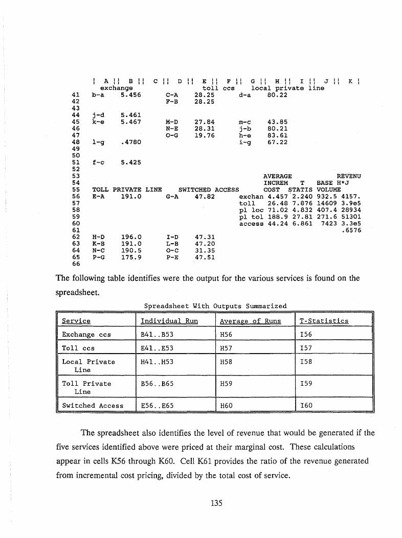
A I I B I I C I I D I I E I I F I I G I I H I I I I I J I I K I I I I I I I I I I I I I I I I I I I I
exchange toll ccs local private line 41 b-a 5.456 C-A 28.25 d-a 80.22 42 F-B 28.25 43 44 j-d 5.461 45 k-e 5.467 M-D 27.84 m-c 43.85 46 N-E 28.31 j-b 80.21 47 O-G 19.76 h-e 83.61 48 I-g .4780 i-g 67.22 49 50 51 f-c 5.425 52 53 AVERAGE REVENU 54 I NCREM T BASE H*J 55 TOLL PRIVATE LINE SWITCHED ACCESS COST STATIS VOLUME 56 E-A 191.0 G-A 47.82 exchan 4.457"2.240 932.5 4157. 57 toll 26.48 7.876 14609 3.ge5 58 pI loc 71.02 4.832 407.4 28934 59 pI tol 188.9 27.81 271.6 51301 60 access 44.24 6.861 7423 3.3e5 61 .6576 62 H-D 196.0 I-D 47.31 63 K-B 191.0 L-B 47.20 64 N-C 190.5 O-C 31.35 65 P-G 175.9 P-E 47.51 66
The following table identifies were the output for the various services is found on the
spreadsheet.
Spreadsheet With Outputs Summarized
Service Individual Run Average of Runs T-Statistics
Exchange ccs B4l .. B53 H56 156
Toll ccs E4l .. E53 H57 157
Local Private H4l .. H53 H58 158 Line
Toll Private B56 .. B65 H59 159 Line
Switched Access I E56 .. E65 H60 I I60
The spreadsheet also identifies the level of revenue that would be generated if the
five services identified above were priced at their marginal cost. These calculations
appear in cells K56 through K60. Cell K61 provides the ratio of the revenue generated
from incremental cost pricing, divided by the total cost of service.
135

Creating Variable Files for the Digital Program
The digital model requires the creation of a different set of variable files.
Because the inputs are different, the variable files can not be used with the digital
program.
We have written a program in UNIX that converts the variable files to dvariabl
(digital variable) files. The program (DVTOOL) is in sub-directory dvarfile. We have
also written a program in UNIX that converts the variable files to dvariabl (digital
variable) files. The program (DVTOOL) is in sub-directory dvarfile.
When running the digital model, the user should use the same combination of
files that were created for the analog model (for example, dvariab1.452 with
populatn.166).
Running the Digital Model
To run the first combination of files (populatn.166 and dvariab1.452), do the
following steps (at the DOS prompt):
1. copy populatn.166 lie .dat
2. copy dvariab1.452 * .dat
3. a. cityinit
b. dxinit
4. digital
5. return
6. choose the level of output--for this exercise, we have chosen level 5.
7. When the program has completed running, you will want to save the results.
Do this by typing
rename digital.oda d452p166.pc
That's all. If you want to look at the results in somewhat greater detail, you may
want to take a glance at file digital.out
136

When you are ready to do the next combination of files, take the following steps.
8. copy populatn.166 * .dat
9. copy dvariab1.453 * edat
10. a. cityinit
b. dxinit
11. digital
12. return
13. choose the level of output--for this exercise, we have chosen level 5.
14. When the program has completed running, you will want to save the results.
Do this by typing
rename digital.oda d453p 166.pc
Evaluating the Results from the Digital Model
The results from the digital program can be evaluated in the same manner as with
the analog program. In sub-directory LOTUS22 you will find the appropriate
spreadsheet (DIGEXAM.WK1). When importing the data (subdirectory digresul), the
user should again start by putting the data in cell A2 (that is, place. the results from
D452P166.pc in cell A2).
The following steps are followed.
1. Go to cell A2
2. IF I N (import number file)
3. D452P166.PC
4. Go to cell B2
5. IF I N
6. D453P166.PC
7. follow the remaining steps for files D4S3p166.pc through D468p166.pc.
8. When all of the files have been loaded onto the spreadsheet, delete all rows
below row 33. This is done by taking the following steps:
a. Iw (worksheet)
137

b. d r (delete rows)
c. a34.z100 (delete area a34.z100)
9. Now we need to load the formulas from DIGEXAM.wkl. This is done by:
a. go to a34
b. If c c (combine file)
c. a34.z100 (define range)
d. DIGEXAM.wkl (define worksheet from which formulas will be obtained).
10. F9 (calculate)
The results may now be analyzed. The reader should focus on the calculations
that appear on lines 42 through 66.
Other Spreadsheets Used to Create Files and Evaluate Results
The spreadsheets that we have discussed up to this point were created so that the
user could get a quick feel for how the model operates. NRRIEXAM. WK1 was created so
that there was only 1 iteration of the model, and no restarts. The following additional files
have been provided:
138

List of Spreadsheets
SJ2readsheet Use
varsmall.wkl same as nrriexam, but 500 iterations, 1 restart and 4 extra 2BESS switches.
varlarge.wkl varsmall can be used to create 17 files. varlarge is set up to create 26 files
vreslarg.wkl Same as analexam.wkl, but used with varlarge.wkl
dreslarg.wkl Same as digexam.wkl, but used with the 26 varlarge and dvtool
stdalone.wkl Creates variable and population files for calculation of stand-alone costs
Correcting for Local Minimum
The search algorithm, the downhill-simplex method, may not locate the global
minimum network configuration. Sometimes the model will select switch locations that
do not minimize the cost of production.
A nonoptimal selection can be detected by using VRESLARG.WK1,
DRESLARG.WK1, ANALEXAM.WK1, or DIGEXAM.WKl. If a negative marginal
cost shows up on these worksheets in blocks A41 to H52, or if the marginal cost appears
to be abnormally high (relative to the other estimates), the data should be further
analyzed.
For example, suppose that when using ANALEXAM.WK1, cell B41 indicates that
the marginal cost of exchange service is negative. For the combination of files that we
have been working with, this would occur if the total cost associated with v452p 166.pc
was less than the total cost of v453p 166.pc. V 453p 166.pc should be greater than
V 452p 166 because the level of exchange usage is higher by 233 ccs (cell B34--worksheet
ANALEXAM.WK1).
139
The total cost reported in file V 452P166.pc could be greater than V 453P166.pc
because for V543p 166 the model found a better location for the central offices. To
correct for this problem, the locations from file V543p 166 are used to determine the cost
of combination V 452p 166. The mechanics for this process are explained in the next
section.
INSTRUCTIONS FOR USING THE RECALCUlATING PROGRAMS
In addition to the nested technology Ilocation search programs, ANALOG and
DIGITAL, we have provided four additional programs which perform some of the
subsidiary tasks of ANALOG and DIGITAL. Two of these programs are ARECALC
(for analog systems) and DRECALC (for digital), which will compute ONLY the cost of
service for a given technology and location--no optimization is performed. These
programs are useful for benchmarking an existing system, or if you are simply curious
about how much a configuration other than the one resulting from the optimization
would cost.
The other two programs are ALOCATE (for analog) and DLOCATE (for digital).
These programs will optimize location ONLY for a given technology configuration. For
example, if you want to know what the cost and optimal location for, say, 3 DMS10()®
switches attached to 3 remote switches would be in a given city, you would run the
program DLOCATE.
The programs run similarly to the main programs; that is, follow the same sequence
of steps with one exception. Prior to the sequence of steps, you must create (in the
analog case) a file called ANALOG.LOC or (in the digital case) DIGITAL.LOC. This
file is formatted as follows:
LINE 1: n (= number of central offices (including remotes)) LINE 2: xl x2 x3 x4
xS ... xn (= switch types of central
offices; see below.
140

UNE3 111 112 (= (x,y) location for switch #1 )
121 122 (= (x,y) location for switch #2 )
LINE n + 2 Inl In2 (= (x,y) location for switch #n )
The switch types are coded as follows. In the digital case, 1 =DMS100;
2=DMS10; and 3 = remote. In the analog case, 1=lAESS; and 2=2BESS.
For example, consider the following digital.loc file.
DIGITAL.LOC
6
133333
12.6825 12.3529
6.0541 5.0482
20.1771 16.9141
19.4684 5.6313
13.1777 20.3409
5.1405 19.7397
The file indicates that six switches should be deployed. The first switch,located at
12.6825 12.3529 is a DMS100®. The remaining 5 switches are remotes, and are located
at,
6.0541 5.0482
20.1771 16.9141
19.4684 5.6313
13.1777 20.3409
5.1405 19.7397
141

Once you have created the location file, follow exactly the steps for either the
ANALOG or DIGITAL program until you reach the last step. For the last step, enter
the name of the recalc program you want rather than either ANALOG or DIGITAL.
That is, the last step is
or
or
ARECALC < Enter>
DRECALC <Enter>
ALOCA TE < Enter>
DLOCATE <Enter>
(for analog cost computation)
(for digital cost computation)
(for analog location optimization) or
(for digital location optimization).
Data Needed to Run the Model
The following data should be obtained to run the model. All of the data
identified in this section is used on a regular basis by the telephone companies and are,
or have been, used in their own cost studies.
1. Carrying charges for the study year. The data should be provided at the sub
account level (for example, the telephone plant index series for underground copper
cable; underground fiber cable; analog switching; digital switching; circuit equipment and
so on).
2. Telephone plant indexes from 1980 through the study year. The data should be
provided at the sub-account level (for example, the telephone plant index series for
underground copper cable; underground fiber cable; analog switching; digital switching;
circuit equipment etc).
The user may want to adjust these carrying charges to reflect higher flower capital
costs.
3. Broad-gauge unit costs for outside plant. The data should be provided for
different gauges of wire (at a minimum, underground and buried cable). In addition,
data should be provided for fiber cable of different sizes (at least ranging from four to
144 pairs-.. both underground and buried fiber cable).
142

4. T-carrier utilization rate.
5. The pair-design standards used for feeder and distribution pair. What is the
design ratio for feeder and distribution pairs per customer (for example, two pairs per
household in the distribution plant, 1.5 pairs per household in the feeder plant, 1.05 pairs
in the feeder plant when customers are served by subscriber line carrier)?
6. Percent of cable that is underground in (a) residential neighborhoods, (b)
downtown district, (c) mixed/residential district.
7. Percent of switched busy-hour traffic that is toll traffic (both interLATA and
intraLATA).
8. Percent of lines that are private line. If possible obtain the ratio for (a)
residential neighborhoods, (b) downtown district, (c) mixed/residential district.
9. Percent of private lines that are toll private lines.
10. Land and building loading factors for circuit and switching investment (the
ratio that is multiplied against the primary investment in circuit and switching in order to
determine the investment in the supporting land and buildings).
11. Main distribution frame investment per subscriber. Obtain this data for both
analog and digital switches. The cost differs by technology.
12. Average busy-hour holding time for local and toll calls.
13. Load coil investment per pair.
14. Tandem busy-hour switching investment per ccs.
15. Current cost of installed conduit/per foot.
16. Investment for conduit used for underground per copper-pair foot (loading
factor for conduit per underground copper pair-foot).
17. Busy-hour ccs usage for business, residential and mixed residential/business
areas.
18. Loading for miscellaneous investment for underground and buried cable. This
should reflect items that are not included in either the broad gauge cost data (# 3) or
load coil investment (#13). Typically this value will be equal to one.
In the chart below, we map which variables should be based on the data provided
in the previous information questions.
143

Information Requests and Variable Names
Request Number variable names 6
One ac211; ac212; ac22157; acess; ae244; ae2422; ae2423; ae815; ae845
Two tpiund80; tpibur80; tpieond80; eondpf; diglOOtp; diglOtp;
tpiosp80; tpi5780 TPIOSP90; tpi5790 tpiundf90; tpiburf90; tpieond90
Three f1526; f1524; f1522; f1519; f4526; f4524; f4522; f4519; m1526; m1524; m1522; m1519; m4526; m4524; m4522; m4519; ufibfix; ufibme; bfibfix; bfibme
Four tuti1
Five fppereust fpslcpereust dppereust
Six perund bus; perund med; perund_res
Seven tol1per
Eight perpl [1] ; perpl [2] ; perpl[3]
Nine pltollper
Ten build22157; bui1d22177; 1and22157; 1and22177
Eleven mdfeost
Twelve intraht; interexeht; to11ht
Thirteen loade
Fourteen tandem
Fifteen feond
Sixteen eondpf -
Seventeen ees_per_res_Iine; ees_per_med_Iine; ecs_per_bus_Iine
Eighteen mise15; mise45
6Variable definitions are provided in the appendix.
144
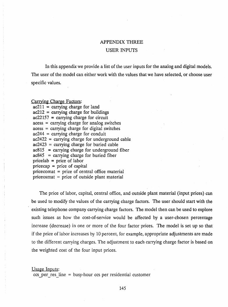
APPENDIX THREE
USER INPUTS
In this appendix we provide a list of the user inputs for the analog and digital models.
The user of the model can either work with the values that we have selected, or choose user
specific values.
Carrying Charge Factors: ac211 = carrying charge for land ac212 = carrying charge for buildings ac22157 = carrying charge for circuit acess = carrying charge for analog switches acess = carrying charge for digital switches ac244 = carrying charge for conduit ac2422 = carrying charge for underground cable ac2423 = carrying charge for buried cable ac815 = carrying charge for underground fiber ac845 = carrying charge for buried fiber pricelab = price of labor price cap = price of capital pricecomat = price of central office material priceosmat = price of outside plant material
The price of labor, capital, central office, and outside plant material (input prices) can
be used to modify the values of the carrying charge factors. The user should start with the
existing telephone company carrying charge factors. The model then can be used to explore
such issues as how the cost-of-service would be affected by a user-chosen percentage
increase (decrease) in one or more of the four factor prices. The model is set up so that
if the price of labor increases by 10 percent, for example, appropriate adjustments are made
to the different carrying charges. The adjustment to each carrying charge factor is based on
the weighted cost of the four input prices.
Usage Inputs: ccs yer _res _line = busy-hour ccs per residential customer
145

ccs yer _ med _line == busy-hour ccs per medium density customer ccsyer _bus_line == busy-hour ccs per business customer perpl[ 1] = fraction of residential neighborhood lines that are
private lines perpl[2] == fraction of mixed neighborhood lines that are
private lines perpl[3] == fraction of business neighborhood lines that are
private lines tollper == percent of switched traffic that is toll traffic pltollper == percent of private lines that are toll lines
(special access) intraht == holding time for intraoffice call interexcht == holding time for interoffice exchange call tollht == holding time for toll call
Outside Plant Inputs: perund _ bus == fraction cable underground, -business neighborhood perund _ med == fraction cable underground, mixed neighborhood perund _res == fraction cable underground, residential
neighborhood plcost == cost markup fraction for private line loops f1526 = fixed investment per foot of underground 26 gauge cable f1524 == fixed investment per foot of underground 24 gauge cable f1522 == fixed investment per foot of underground 22 gauge cable f1519 == fixed investment per foot of underground 19 gauge cable f4526 == fixed investment per foot of buried 26 gauge cable f4524 == fixed investment per foot of buried 24 gauge cable f4522 == fixed investment per foot of buried 22 gauge cable f4519 == fixed investment per foot of buried 19 gauge cable m1526 == marginal investment per pair foot of underground 26 g. m1524 == "" """ II" 24 II
m1522 "" "" "" II 22 II
m1519 19 m4526 "" Ii""" buried 26" m4524 24 m4522 22 m4519 19 ufibfix == fixed investment per foot cost of underground fiber ufibmc == marginal investment per foot of underground fiber
(per fiber) bfibfix == fixed investment per foot cost of buried fiber bfibmc = marginal investment per foot of buried fiber (per
fiber) misc15 == miscellaneous investment related to underground copper misc45 == miscellaneous investment related to buried copper
146

looputil == utilization of copper loop line capacity blockwidth == width of city block, in kilofeet loadc == 1990 load coil investment (per copper pair) fppercust == feeder pairs per customer copper wire fpslcpercust == feeder pairs per customer, slc-96 dppercust == distribution pairs per customer fcond == cost per foot of conduit (total investment) sic_mode == SLC-96 mode, 1 == unconcentrated; 2 == concentrated
The fixed and marginal cost of outside plant is obtained by
running a linear regression: cost == A + B * cable size.
Where:
A == the fixed investment per foot of cable
B == the marginal investment per foot of cable
Central Office Inputs: dmslOOcap = calling capacity of a DMS100 digital switch dms10cap == calling capacity of a DMS10 digital switch aess1cap = calling capacity of a 1AESS type analog switch bess2cap = calling capacity of a 2BESS type analog switch remotecap == ccs capacity of remote switches max remotes == max number of remotes attachable to DMS100 coleceng == central office tel co engineering analog switches switchutil == utilization of switch capacity build22157 = investment loading for building, applied to circuit build22177 = investment loading for building, applied to switch land22157 = investment loading for land, applied to circuit land22177 == investment loading for land, applied to switch cbd factor = multiplier for land in CBD meddens factor == multiplier for land in MDD lowdens _factor = multiplier for land in LDD mdfcost = main distribution frame cost per customer (separate
values analog and digital switch) tandem == 1990 tandem investment per ccs. tutH == t-carrier utilization factor min _ 2bess = minimum number of "extra" 2BESS machines tried in the analog model.
147
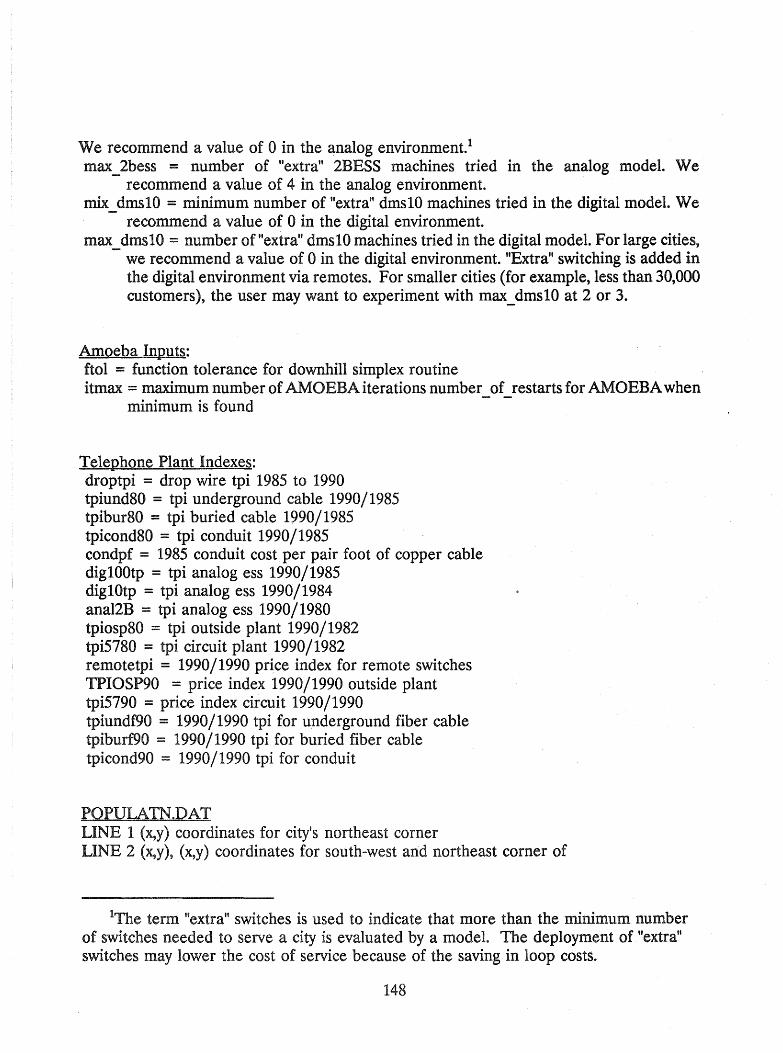
We recommend a value of 0 in the analog environment.1
max 2bess = number of "extra" 2BESS machines tried in the analog model. We recommend a value of 4 in the analog environment.
mix dms10 = minimum number of lIextra" dms10 machines tried in the digital model. We - recommend a value of 0 in the digital environment.
max dms10 = number of "extra" dms10 machines tried in the digital model. For large cities, - we recommend a value of ° in the digital environment. "Extra" switching is added in
the digital environment via remotes. For smaller cities (for example, less than 30,000 customers), the user may want to experiment with max_dms10 at 2 or 3.
Amoeba Inputs: ftol = function tolerance for downhill simplex routine itmax = maximum number of AMOEBA iterations number of restarts for AMOEBA when
minimum is found
Telephone Plant Indexes: droptpi = drop wire tpi 1985 to 1990 tpiund80 = tpi underground cable 1990/1985 tpibur80 = tpi buried cable 1990/1985 tpicond80 = tpi conduit 1990/1985 condpf = 1985 conduit cost per pair foot of copper cable dig100tp = tpi analog ess 1990/1985 dig10tp = tpi analog ess 1990/1984 anal2B = tpi analog ess 1990/1980 tpiosp80 = tpi outside plant 1990/1982 tpi5780 = tpi circuit plant 1990/1982 remotetpi = 1990/1990 price index for remote switches TPIOSP90 = price index 1990/1990 outside plant tpi5790 = price index circuit 1990/1990 tpiundf90 = 1990/1990 tpi for underground fiber cable tpiburf90 = 1990/1990 tpi for buried fiber cable tpicond90 = 1990/1990 tpi for conduit
POPULATN.DAT LINE 1 (x,y) coordinates for city's northeast corner LINE 2 (x,y) , (x,y) coordinates for south-west and northeast corner of
lThe term "extra" switches is used to indicate that more than the minimum number of switches needed to serve a city is evaluated by a model. The deployment of "extra" switches may lower the cost of service because of the saving in loop costs.
148
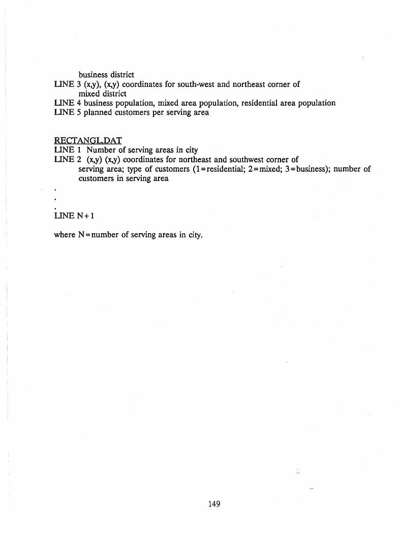
business district UNE 3 (X,y) , (x,y) coordinates for south-west and northeast corner of
mixed district UNE 4 business population, mixed area population, residential area population LINE 5 planned customers per serving area
RECfANGL.DAT UNE 1 Number of serving areas in city LINE 2 (x,y) (x,y) coordinates for northeast and southwest corner of
serving area; type of customers (1 = residential; 2=mixed; 3=business); number of customers in serving area
UNE N+l
where N = number of serving areas in city.
149
