United States Deparlt m ent of Estimating the Economic Impacts Agriculture of Recreation Response to Resource Forest Service

s ~ i S v sew<, Management Alt errlat ives @ *rtsia la-+

Southern Donald B.K. Erlglisli, J.M. Bowker,

Research Station J01~1 C. Bergstroln, and H. Ken Cordell

General Technical Report SE-91

The Authors:

Doriald I 3 . K English and J . $1. Rowker arc Rescarch Social Scientists (ICc~norrlists)~ USDA Forest Service. Soutiiern Research Stat ion, iitliens, G A ; John C. Bergstron~ is Associate I'rofessor, Department of i4gricultural and Applied Econorriics, Urlivcrsity of Georgia, iitherts, GA; and 11. Ken Cordell is Project Leader, USDA Forest Service, Southern Research Stat ion. Athens, GA.

April 1995

Southern Research Station P.O. Box 2680

Asheville, NC 28802

Estimating the Economic Impacts of Recreat ion Response to Resource Manage ent Alternatives

Donald B.K. Englislr, J.M. Bowker, Jollri C. Bergstrorn, arrd 13. Kcrl Cordcll

hlatlagillg forest resources itivolves t raclcwffs aticl ttiaking decisiotls aniotig resource 11ialiagcttlc.rlt nltcr ixatives. So111e alterriativcs will lcatf to clla~igos it1 t11c levcl of recreatiorl

\.ititittion ant1 tlie anioultt of n*sot:intc~tl visitor spetlclitlg.

l'iins, tlie alter~xati ves call affect local ecorioiiues. This paper reports a itlethod that car1 be useti to es t i~nate the

econoituc impacts of such alter~iatives. hIt>tlrucls for derivi~rg representative final deinariil vectors and for e\t ilil,itittg

visitation I . C S ~ ) O I I S ~ t o ~ t i ~ ~ i i r g ~ i t i t ' t ~ t a l t ~ r ~ i a t i w s iile preser~ted. Tltese irletltocls are illustrated i t i t w o etiil>iiic<il c.t,rtiiple~ tliat involve tlelayit-ig water-level ~ I ~ L H < ~ C > W I I iit ~lioi~tttiiiil rese~-v~lirs. Otie exal i~~ple is for four reservoirs i t 1 wcstert~ Nortli C:aiolina;

tlie otlter i s for two reservoirs i t i ~~or t l rc t t i California.

I<cywortIs: l<coiio~nic iii~j)act, recreation, reservoir level, resotlrce i i~anngct i~ei~t .

In t roduct ion

Ili devclopirig ancl artieritling ~iiari:tgertietit plans for their forests, planners for the National Forest System (NFS) account for the coriseqr~er~ces of proposed ~l~anagertiet>t clta~iges on tlte forests ant1 their users anti the surrouxicli~ig cornr I lrtni ties. Itecently, attent ion 1i:ts foctlsed on c11:tnges in recreat,ion ol:j~orturtities anti their ef ic ts on local economies. r , l liis paper tlcscribes n. gc'neral ~ilethoci to estimate the regiorlnl ecorio~nic inipacts of resource rnatlagernent alttrnatives. Two stuclics 011 the reiativrlship aniorlg reservoir leveis, recre;ttiori use, anci the local ecorlorrly illrlstrate r~letltod al>pIicatio~i.

Theoretical Backgrounc!

Regionaf econonlic ir-npacts of a project or policy are the clianges in the ecorior~iic activity within the region thac result from that project or policy (Randall 1987). Regional economic impact analysis focuses on

esogeriot~s ch;tnges in final ciemancf for goods and services prodtlceci in that region (Stevens and Rose 1085). Impacts include and are often rneasured in c l ~ a n g ~ s in the real value of industrial output (goods ancl services), ernployrilent, and proprietor and lioriseliold iticoilie the region (Sassone and Scltaffcr 1978). Most ecorlornic impact is assessed tltroilgil sorilc for111 of general cquilit>rium model. S t,;irti~lg fro~tl all initial etluiiiLrirtlri, these ri~odels itssilrrle ;tn c~xogctions cf~a~lge car~secj by the policy or project ii~lticr study and crtlcitl;it,e tlie resulting 1iyl)otlietic;~l c~cji~ilibriuri~.

' lhe direct, ir~tiircct, and induceci effects of the exogenous cllarige represent the total economic impact ( R icli~tr~lson 1973). For example, when recreation visit:ttiott iiicrcases, direct effects are the first-round pi1 rcI~:~wsi~l ~:t(le by bttsinesses to 11ieet the increased tlc~ri;i~itl for t lieir products by recreation visitors (I3clrgstrori1 ai~cl otllers 19'30). I~ldirect effects occur :is tile first-roi111t1 inp~t t st~ppliers ri~ake adclit,ional 1)i1rclr1ases to riieet iricreasecl clcrnands of their clients. 'l'lie clircct arid indirect efrects result in an overall prociuction increase that can lead to rriore local or regional etrijjloyrrlent ancl income. As residents spend their itrcreasctl inco~xe~ further rounds of economic activity are generated. These are the induced effects.

Regionztl eco~torriic irtnpacts of recreatiorl are based primarily otl visitor exj3enditures associatecl wit11 tile l l ro i l \ ic t iori of recrr:ztion trips. The money tliat vihitors hperltl for itfirtls such as food, lodging, ancl tr;tr~spor t i t t ion hecort~i.s ft~el for the local ecotrotriy. hl;znagerr~e~it aIternatives that affect the an~otlrit or type uf Inoney spcnt will then affect the focal ecoiiorrly. \'C'hcn assessing ecorloniic impacts, recreation is considered a basic exporting industry; titerefore, only nonresident expenditures are included. Resident spending for recreation trips within the

regiori re1)resc1tts a transfer of rlioney within the region anti does rtot corttrik,ute to econor~~ic growth (t2lw:trci ar~ci 1,ofting 1985; 13ergstrorr1 arlci ottiers 1990; I3ockbt;~c.l i t r t t l 3lcCor11ic.11 1!I)X 1 ; CorcIcll artrl otltcrs 19'32; I,ical>er a11tl ot ttcrs 1989).

Ex post verification of the psedictiorls developecf from these neth hods is seldom done, often for the same reasons that initial baseline visitatiorl ctata are not collected.

Ifowevtar, ;L I I I ; L I ~ ; L ~ C ~ I I C I I ~ ; ~ l t ( ~ r ~ ~ i t f i v e ci11i c;titse rcsi(1cr1ts tc:, switclt t rilt cl<t:,t,i~~;ttio~~s fro111 ;I bite o~ltsiclc t llr rcgior~ to on<. i r ~ s i c l t . t lic rcgio~t. \liltcr~ this occurs, t l ~ e rc.gio~l;ll cco~tnrt~y cxpt~rit~rices a rcductiott in its irnyortirtg of recrcatiorl service (less local 111olley '1e;tks' out of the ecoriorr~y). 'I'lie ovc1r;ill result is a net ir~crcase i r r trtoney spcr~t ort rc.crtb;~tiorl i t 1 tllc local

r \ ecortorlty. 1 l~cse switc1rr.s i l l clcstir~;ttioli procfilce ;t

positive economic impact; however, most studies (lo not include them.

Method

To estimate the regional econornic impacts of a resource ~nanagement alternative, a planner must have three sets of information: (1) an indication of the magnitude of the changes, based 011 the expected size of the visitation change, positive or negative, for each alternative; (2) an indication of the nature of the changes for each alternative, measured by some summarization of the profile of expenditures rnztde by the various types of recreation users; anti (3) an economic model of the target econorny.

Visit at ion Changes

Accurate estimates of visitation response to resource management alternatives is oft,en the lliost ciifficult i~lformation to obtain or estimate. &lost pul>lic agencies do not collect visitation data a t their sites. The dispersed nature of niany ac tivi tics ancf the variety of access types and locations usually rliake collecting this data proliibitively expensive. Thus, baseline estimates of current recreation use anti how use varies over the year frequently rely on gerieral observations by managers and field personnel.

Estimating visitateion changes resulting fro111 resortrcp management changes is even more difficult. Such estimates can be developed through user surveys, expert panels, or behavioral models. Unfortunately, the nonmodeling methods rely on individuals' opinions about contingent future states and are often considered far less reliable than behavioral models.

Current users can be surveyed for their expected-use levels in different management scenarios. Somewhat expensive, this method is subject to strategic responses by users and does not irlclrltle potential response from nonusers. This method could provide a lower bound to visitation increases, since visitation increases from current nonusers would not be incluclcd.

Expert panels are groups of individuals knowledgeable about the site, its resource attractiveness, arld its rise ~);tttertts. 'I'liese prznels can be asserlibled and :tskecl to esl i l l late aggregate visit atiorl response to select cd 13 t;tri;~gc~rierit or resource cllanges. This r~ietlloti 11t;ty also be susceptible to strategic behavior, a~tci its results are uot always considered reliable by rt-rn~l;tgcrs, policy makers, or rcsearcliers.

i2lotlt~li11g eittails predicting aggregate changes in trip I>el~:tvior of recreating ~touseltolds within the market arca of t hc. site in response to cllar~ges in management ;ict.ion. Accliliri~ig sufficie~tt data for these rnodels call be cxpc~isive. In acidition, detert~iining i~cctirate visit;ttio~i-resl)ot~se rrieasures can be quite cott~ples, because site demarid in most inodels (1~j)encis sir~l~ilt;trleously 011 the availability, quality, iind prosinlity of both target arid substitute sites (1~cscri11i;tier and Leiber 1985; &lcCollurii and others 1990). \iritllout good baseline visit,ation data, models of site clerriar~tf (see, for esarttple, li_'i~n and Fesenmaier 1990; I'ctersorl a11ci others 1983: Peterson and others 1985) that include resource ainoiitits or quality levels i \ > s i t ~ - ~ i c r t ~ i \ ~ ~ ( l pre~lictors c;tiiliot be tlevelolted.

Iloir~vt.r, gt.~~c.r:tl rtiotlcls of rccrcation cler~laritl caIl l ~ e tiscti to ifcvtllop c3titli;ltc.s of possillle cllariges in recrcat ioil m e or visit ittioll oil ti;itio~l;tl forests in rcsj)olise to proposed ~~ l r t i~ngcmcr~ t cl-tanges. National and rcgional ~ t ~ o d e l s of recreatiorl denland have been developccl for use in the Forest and Rangeland Renewable Resources Planning Act of 1974 (RPA) (Corticll aitcl ot licrs 1990; English and others 1993). 'l'liese niodels estimate the total number of trips ernanatitig from an origin without regard to the destiitation.

13y tlsiiig reporteci coefficients for the explanatory varia1,les for rricreatioil corlsurrtlition (Er~glish ancl otllcrs 1993) and valt~cs for those variables ap~xroiwri;ttc to tlie r11;irket area of the forest, ari esti~riate of tot;tl trips gcricrateci from that rnarket area can be o i j t a i~~ed . Ctlartges in tile number of geliierated trips per unit c11;tnge i n resources can also be calcirlatecl by rcisource v;iriable. hlultiplying the c l ~ a ~ l g e i t ) trips pc.r r ~ r i i t c l~a~ ige i r i resources by the size of e;~cll resourcc cliai~ge ~)rol>osed in the r~~arl;tgcrr~erit ;tlteriiativc yic'lils tlit: clrange in total nnnil,cr of t'rips generated i i t tlie rriarki~t area caused by the proposed alterr~ative.

The two approaclies that detcrrrline how rriarly of these total trips occur on the forest are based on different assumptions. First, because the only resource change is on tlie forest, one could assurne that all increases or decreases in trips will occur on the forest. This approach also assllrtles that no location or activity substitution occurs. For example, if a forest increases the amount or quality of a resource, additional trips to the forest are assumed to come only from new trips generated in the area. No increases will come from people switching destinations from another site in the area, such as a state park, or frorn people switching trip activities to take advantage of the improved resource base.

A second, rrlore conservative approach is possible if estirliates of current forest use are available. With this inforn~rttion, the forest's rriarket share of trips can be calculated. Assuming this market share remains const;trit, the total-trip increase on the forest is equal to the ~,rotluct of the total-t rip increase in the rriarket area ant1 the rwtrket stlare fraction. Tliis approach leacis to less volatile changes in recreation use when cotnpnred witti t Ile first approach.

Total filial denlalid cfiallgcs for a resource managerncnt nl t ernative are cfeterr~iined by rr~ultiplyirlg the cllange in the niirnhcr of trips for a riser type by the per trip vector of sectorial final dernancl changes. The result is the set of final clernarld event changes rlseci as input for the IRIPLAK rnocfel of the target econoniy.

Vis i to r E x p c z l d i t t ~ r e

Ex13enditilre cfatzt for visitors to a site or area are not alivays readily availabie. Froin 1985 to 1989, the Ptiblic Area Recreation Visitor Study (PARVS) collected expenditure data for a variety of Federal locations in the Southeastern United States. Since then, a similar survey method, entitled CUSTOMER, has been used to collect expenditure data for particular types of users a t USDA Forest Service and USDl Bureau of Land hlanagetrient sites. The data frorn these surveys may be reasonably representative of the entire set of users of national forests and other public lands irl tlte Southeast. IIowever, the s a n e is r ~ o t getierally true for the remainder of the country, primarily because the amount of data collected is inadequate and CUSTOhl ER sites are self-selected.

For site-level analysis, the best data is collected by interviewing a random sample of users a t the targeted site. If site-specific data are unavaitable, expenditure data frorri silirilar, nearby sites could serve as proxies as long as plaliners use their knowledge of the rcsotlrce area to cleterrt~ine if applying proxy-site data is appropriate. Because expenditures for tii ffereri t cor~inlodities can have different types ;tnd levels of impacts on local economies, obtaining experlditure data for major expenditure categories is recommended. Examples of these categories include public and private lodgi~zg, food and beverages bought a t stores, food and drinks bought a t restaurants and bars, gasoline and oil, recreation services (such as guides or equipment rentals), sporting goods, souvenirs. and clothing.

Regardless of the source of the expenditure data , the j~rofiles of expenditures made by different user types n ~ u s t be sritnrliarized. The most common summary is tlie average arnount spent per person per trip. Itlclutiir~g rt co~lfiderice interval is also recommended, so the range of expected irnpacts can be estimated. I f the clistribu tion of expentiitures is Iliglily skewed, the median may be a more appropriate summary stitfist ic anti a rioriparametrie confidence interval may be estimated (Bo~vker and LIacDonald 1993).

I f the sarnpling plan irlvolves a random survey of visitors 0 1 1 site, visitors who stay longer may be sanijjled niore than those wlto stay for a shorter time. tt'hen this is the case, an appropriate weight rt~ust be assigned to each observation. A weight

suggested in tlle past for similar research applications is norrilalization by the muitiplicatiw inverse of stay length (Scllreuder and otliers 1975).

Iterns bougf~t by visitors are usually compatible with the c o ~ i ~ i o d i t y sectors in the IhlPLAN model. Sometimes, margining of reported exp eriditures by category is necessary, especially if expenditure data is aggegated into ~ n a j o r categories. The allocation algorithm reportccl here is used by the Soutlrer~i Research Station arid is based on riatiorla1 annual personal constrlriptio~i espetiditure data and input-output tables preparetl by the Bureau of Econornic Analysis from 1987 (table 1). AppIying the sectorial allocatiorl algori thnl to the expenditure profile for a visitor type yields final-demand changes by IMI>LAN cornrnodity sector for that visitor type, measured in dollars per visit.

'Fable 1 has two comlr~odity allocations for food arlcl beverages bought a t stores, one for visitors engaging in developed activities and one for visitors engaging in dispersed activities. This represents the authors' views that the market basket of food goods is different for these two groups. For example, those engaging in developed site activities, especially carnpers and picnickers, often use perishable, high-weight goods, such as ice, fruit, fresh meat, and milk, that visitors participating in dispersed activities are less likely to consume.

Econon-lic Model

Many studies of the economic impacts of recreation visitation have used input-output models to simulate the regional economy. The USDA Forest Service I 0 model, IMPLAN, bas been modified to better estimate the effects of recreation visitation. The advantages and disadvantages of IMPLAN have been widely discussed (Alward and Lofting 1985; Alward and others 1985; Bergstrom and others 1989, 1990; Cordell and others 1989, 1990: 1992; Hotvedt and others 1988; Propst 1985).

In previous studies of the economic impacts of recreation visitation, the size of the regional economy hcas ranged from single communities to entire States. Planners often delineate the target economy as the area that includes a11 counties that physically include part of the management unit undergoing plan development or amendment. For example, when

exanlining ait,ernatives for a Forest Plan, the target econonly would include all counties that contain a yortiorl of that national forest.

Empirical Examples

The two empirical studies described in this section illtistrate method application. Both are about recreation-visi tation response to proposed changes in 111anaging water levels in reservoirs during the recreatiorl season. Both st~lcfies used similar data collection ri~ct,hocis. During the recreation season, exit interviews were conducted on a stratified random saniple of reservoir users. St ra ta were selected to represent major user types according to expected differences irl expenditure pat terns and visitation response to rlianagement alternatives.

Data collected a t the site iricltided visitation and travel patterns. Respondents were asked to give their atl(lress for a follow-up mail survey, which would incluclc, trip-related expenditures, recreation equipri2ent pirrcliases in the past 12 months, and equipment-use patterns. To collect expenditure data , one study used the PARVS instrument; the other used the CUSTOMER instrument. Survey procedures followed Dillman's (1 978) method.

Trip-related expenditures within the general categories of food, lodging, transportation, activities, and other were divided into three groups: those made a t or near horne, those rnade en route to and from the site, and those made a t or near the site. For equipment purchases, such as recreational vehicles (RV), boats, and related accessories, respondents reported total expenditures and the portion of expenditures occurring in their horne county. Only expenditures made in the local area by nonresidents were relevant for cletermirling economic impacts. Methods for allocating i>otli trip-relatcil and annual equipment expenditures to the local area have been developed through the cooperation of government and academic researchers (Propst 1985; ?Vatson and Brachter 1987).

All trip-related expenses made a t or near the recreation site were assumed to occur within the impact region. Trip-related expenditures made a t or near home were assumed to be rnade outside the local impact region. En route expenses were assumed to be equally likely in each mile traveled. Further,

it U;LS ;t~sl~rri(:d that visitors would take the most tfircct rotite possible to tile visited site. A straight Iirle fro~rz ho~rte to site was cafculated for each visitor, arici the poirtt where ttlis line entered the local impact regiorl was rioted. 7'he ~~roportion of the st'raight line lyir~g \t?itllin the irnpact regiorl equaled the expected percer~tage of a11 en route expcinses occurring in the local region.

E<~ui~xitent pirrchases tiot rn;ttic. i t 1 tile resl~or~clent's horne county were spati;tlly al1oc;ttetl based on ecltiiprrtent-rrse ~)at t~er~ls . It was ;tssur~led that the ~,~irclt;ises ~ i o t itlade 1lc;tr llor~re were ri~ade dtiring a recreatiorl trip.' Arlti1t;tl spentlitrg for each ecliiiprrient type was divitfed by the r~tlriil~er of trips on which tile ecj~~i i>~i t :ut was used i r t t,11c 1;tst 12 r n ~ n t ~ l ~ s . This ~ti~rrlbcr was tt1111til)licd by the ratio of equiprrient rlse at the visited site to total equiprne~lt use. The result was t11e expected arinual equipment purctiases in the region attributable to recreation trips to the specifietl site.

W e s t e r n N o r t h Carol ina

I'ressnres fro111 rnatly sources, i l~clr~di~tg rccrcntlior~ risers arid recrc;itiort-relrtt,1.d I)nsines~cs, have ca~iseti the Tennessee Valley Art tliorit y ( I ' V A ) to exarrlirie the effects of :tlternativt w;tt txr I~~vcl-trt;ti~agc~ric~it~ policies a t selected rcscrvoirh. 111t crcst lias cc~ltcrcd o t l

the regional ecotlotr~ic itt11);icf s of ~xpccted it~creiises in recre;tt,io~~ ir i rcspoirsc to l~igl~cr srllrrrllcxr water levcls at four reservoirs i l l tire trtoutltains of North Carolina--L;tIies Cl~nf~rtgc~, Foiltatla, tliwassee, and Santeetlall."

'Tl~e TVil Iias rt~nnagecl tlic water lebcls in these reservoirs for flood control a110 l~yclropower. Water levels peak iri late spring as the reservoirs capture runoff frorn December tlirougli April. Water levcls are drawn down frorn early srlrnrner until late fall to generate power and to establish excess reservoir capacity to capture runoff. This policy involves tracicoffs with recreational use because

I B L future studir.~, consicleratio~ls and lrlodeiiilg of cfurnlilc cqtiip~-rlc*itt cxpclldit urt.3 made nway fro111 home on rtor~recreatio~~al t i i rvox~lct be desirable.

drawdowri results in exposed banks, reduced aesthetic a~>peal, and reduced access for boating, fishing, and

Bot11 reserkoir ilianagers anti local business people agree that recreation visitation decreases as water levcls tfrop (i l f lanta Jour?laf-Co~zslzlutzon 1991). The primary reasons for decreases in visitation are reduced surface acreage and access. Normal reservoir operation patterns reduce surface acreage by over 20 percent at tllree of tflie four reservoirs. By August, ttl;tuy ]>oat r;t1nps are unusable, rnany houseboats are str;tntled, ar~tl riiariy coves with submerged rocks are haz;trdous. 13xposed steep slopes (up to 35 degrees a t Fotitanrt) ar~ci large rntid flats surrounding the water, csj~ecially at C:Iiat,iige, ltat~iper foot access. The 211 ternatives being considered involve holding water lrvels tiear fu l l for 1, 2, or 3 rliore rnonths of the year. 'l'liose altert~atives will be referred to as Alternatives 1 , 2 , ;trrcl 3, respect,iveIy.

Visi ta t ion Cllanges. The irnpact region included six cortrlties in westerrl North Carolina: Cherokee, Clay, Gr;tll;tt~i, h1;ic011, Jitckson, ant1 Swain. In 1988 and 198'3, tlitta were collectecl frorn hlay to September. Strata were tlefir~etl by four user types: day, overnight, boat iiig, ant1 tlonl~oatitlg. Overnigllt users spend illore trinie o ~ t site tflali clay users per trip, and they ~)rlrcl~:tse tileals ant1 lodging t411at day users do not. I3oat ers' expericli tures were expected to be higher than ~ioiiboaters, reflecting the additional costs of boat use. 13ecatise boaters' activities are more directly affected by ~vater levcls, their visitation increase in response to rnatiagernent alternatives was expected to be greater than for rtonboaters.

'1'0 est itlrate the ecoriorriic impacts of policy changes, t.sti~~trtt cs were ncecied of visitation changes resulting fro111 ;ilternative reservoir rnanagernent policies. First, tot a1 cftn~ige in visitat ion was estimated at c:lc!i lake ririrler each ~nanagement alternative. Two

sources provided data: current users arid an expert pa11eI. Current users were asked in a mail survey c~ucstiorirlaire how often they visit the lake and how often they anticipate visiting under each management alternative. This represented the lower bound for visit ation change because it assumed no visitation increase frorn new visitors to the reservoirs.

it tietn;fciI tfcsc~ iptiuii of t 11e s t u d y l,,ickgrourlcf, ~nn t~age~ i~e r i t op t i t~~ i s , aritf da t a collectioil can be found in Cordell arid Ber-gst I oil1 (7 993).

Second, an expert panel assigned to each lake was asked to estimate the anticipated percent change in visitation for each user type when cor~lparing current rrla~lagement policy to each managemerlt alternative. The panel considered two sources of increased visits: (1) new visitors to the reservoirs, and (2) increased numbers of visits by current users. "'Expert panel" estirnates represented the upper bound.

A ~nicitile visitation-change scenario was calculated as the mean of the upper and lower bounds. This ~niddle scenario was used for the irnpact example. Total expected changes in visits were developed by ~ r ~ ~ ~ l t i p l y i ~ i g tlie percent clinnge by tlte baseline visitation for each user type ;it each lake. Because tliis study was only concerrleci with increases in noriresiclent visitation, expected total visitation increases a t each lake were lnultiplied by the proportion of rior~local visitation in the current sample by lake and user type. The proportions ranged from 22 percent for day nonboaters a t Santeetlah to 93 pcrcetit for overnight nonboaters a t Fontana.

In ternis of percent, visitation a t Fontana and I(iivassee was expected to be the most responsive to water level changes. Interestingly, current tn~iilage~rlerit practices have the greatest irnpact a t these two reservoirs (table 2). Current management a t Fontana draws water down 45 feet below the full level. IIiwassee undergoes the greatest loss in surface area from the full level (33 percent). Santeetlah has limited access facilities, which may explain why its visitation was least responsive. Estirnated increases in visitation were as expected across user types. For all lakes and management alternatives, estimated percentage increases for boaters were greater than for nonboaters, and estimated percentage increases for overnigllt users were greater than for day users.

The absolute magnitude of the estimated increases in nonresident visits for each Iake and user type is presented by management alternatives in table 3. 1Iolditlg all four reservoir water levels near the full Ievel 1 month longer could result in an additional 320,000 visits, of which about 130,000 could be overnight visits. Keeping water levels near full for 2 additional months could yield 640,000 more nonresident visits, of which about 255,000 could be overnight visits. Maintaining near full water levels for 3 extra months could result in 1.08 million more nonresident visits, of which over 455,000 could be overnight use.

Expe~lditures. The average expenditures in 1988 dollars per person per trip in the six-county area ranged frorn slightly more than $21 for day users a t IIiwczssee to just under $130 for overnight nonboaters a t Foritana (table 4). Overall, between one-half and two-t ilirds of trip purcllases made in the local area were for food ancl lodging. GeneraIIy, boaters spent rtlore per trip in the local area than nonboaters, notably for transltortation and activities. Overnight users spent lliore than ctay users, primarily for lodging :in ci fooci.

Ecollollric Impacts. Economic changes were i~~castired in 1990 clollars. Table 5 presents the ciiangcs in the total indtistrial output, income, and ntilnl~er of jobs in the regional econorny resulting from 1,000 trips l)y nonresicterrt,~ of each type of user at each 1;ike. I~npacts vary by lake and user type: the s~~iit l lcst irt~pacts fro01 day users of Lake Santeetlah ;intl tlie largest i~npacts frorti overnight nonboaters a t I,;lke Fontana. For eitctl user type, visitors to Lake Fo~it :LI~:L gerleratccl 11igl1er levels of regional econonlic i~~ip:icts than visitors to the otlier three lakes.

hlultiplying the visitation increase by the response coeflicicnts for each lake and user type and then s t i ~ n l ~ l i ~ t g user types yiclcls the total impact to the local area fro111 recreation increase associated with e;icii ~ii;inagcnle~it alternative a t each lake (table 6). 'l'lic tli frt>rences in i~npac t resy onse across the four Nortll Carolina reservoirs suggest that the method ~trcscrlted in this paper can be useful in developing policy to facilitate rnult,il,le-objective operation of resources, such as reservoirs operated by TVA i l l ivcstern North Carolina. Lakes Chatuge and Fontaria have a reiatively fligh degree of recreation infrastructure development and current visitation. Lakes Itliwassee ancl Santeetlah are essentially undeveloped areas. Economic responses to visitation increases were generally greatest a t the more tieveloped reservoirs. 'I'fiis suggests that an efficient way to affect local econorr~ic development through recreation rriay be to focus agency efforts on higher stirrlrtler water levels a t Lakes Chatuge and Fontana.

Northern Ca l i fo rn i a Table 7 reports the regressioll model estimates, based ori 'LO years of da ta , for Shasta Lake. As indicated by

T h e local impact region for this s tudy included Stiasta a n d 'l'rinity Counties. The effect of charges in wztter-level rna~iagenient on several key indicators was estirriated for Shasta Lake and Trinity Lake using a rnoclel t h a t integrated a visitation prediction model, the I hl I'Lt1N rnodel. and supy>lenientary projections fro111 ati exper t panel.3 111 addition to the tliree p r i~na ry ecor~ornic iridicators of total industrial output ('1'10), to ta l incorne (T I ) , a r ~ d employrrient in full-tirt~c equivalents (Frl'E), two otller indicators, final dcn~ant l (Fl l ) arid value added (VtZ) were also iricludecl.

Data were collected frorrt May to September of 1992 rtsirig tlte GIJSrI'OM E R ir~str t~rrient . S t r a t a were cf(xfir~cd by fivc prirnary user types a t each lake. For S11;tsta Lakr: tlic c;ztt.gorics ittclntlt:d liouseboating, ot,ltcr b o ; ~ t i ~ i g , t levelo~~ed c;trripirtf;, dispersed carnpirig, ; t r ~ c l fisiiir~g. For 'liittity 1,akt. t11t: categories were tiotrsel~oating, otlier l>oiitir~g, tlcveloped camping, fislritlg, arid scet~ic tlrivirig.

V i s i t n t i o u Cllallgcs. For this s t ncly, detailccl Uurcau of 13eclarnatio1i water-1evt.l cl;tt,a for both lakes a1it1 USDA Forest Service visitatiorl da t a were usecl to develop linear regressio~t v i ~ i t ~ a t i o l ~ rrtodels for eacli lake. i1 rlnual visi tatiorl in tliousand recreation visitor days (ItVD) was specifietl as a fi~rlctiorr of water level a t the beginr~irlg of tile recreation season (May for Sltasta Lake arld June for 'l'rinity Lake), the arnount of clr:iwctown hctweeri t,lir water level a t the beginni~ig of the seasori ancl Septerr~ber, arid a tirrle trend to reflect a treri<l in recreatiorl t;tstes and preferences. 'I'tic Shas ta Lake visit;~tio~t ccluaticrn is specified as

b,, 1-,I . . . = regressior~ coefGciertts, In = tlie natural logari t l -~rt~, Rlaj = tnearl hlay water level a t SIiasta Lake for a

give11 year i l l feet above sea level, I3rolt = t ha t year's drop in feet of tlie average

ino~ttllly water lcvrl fro111 ,"\lay t o Seitt,erliber,

Year = tllc Y C ; L ~ of observ:ttion, ar~ci u, = the randoill disturbance term.

t11e ft%tatistic, the estirllated model explains more tliarl 90 percent of the variation in observed visitation. All of the explanatory variables are highly significant with irlttlitively plausible signs. Annual visitation is positively affected by higher water levels in May. T h e Ycar coefficient is positive, indicating tha t when other factors arc llcld constant, recreation visitation has I,c.en ir~creasirig over tlie past 20 years. Visitation is ilcgatively infiuenced by drawdown in the water level during the recreation season. Elasticities, representing t lie percent cltange in visitation resulting from a 1 perccn t cllar~ge i l l explanatory variables, are also rcporteti.

For S1t;~st;t Lake, pretiictecl visitation ranges f rom rot~glily 1.7 111i1lion RVD uncler the drought baseline to aljout 3.9 rliillion ItVD rrrtder nonclrought i~ltcrtt;ttive 2 ( table 8). 111 a drought season, I I I ~ L I I ; ~ ~ ~ I ~ C I ~ ~ cliitnges c;trt effect a 10-percerlt increase i lk vihitiztioll I)y restricti~lg seasonal water drawdown to it I I I ~ I ~ ~ I I I ~ I I ~ I ;ts reproseritccl l ~ y al ter~lat ive 2. In rioritlrot~gl~i cori(litiot~s, tlic nuniber of arinual RVD ii~i'rc~;tst~:, tir;~~ti;zticitlly j)rit~iitrily because of the ii~crc;tsclcl watclr 1t.vels i l l 3Iay. It1 this case, restrictitig tlri~wclo~vrt to ;I i i i i ~ ~ i r ~ i r r r ~ r (a1tt~rn;itive 2 ) would lead to art iricrc.asc. i l l visitation of about 25 perccnt.

'I'lic 'I'rini t y 1,itke visit itti011 rrlodel was siritilar t o t ltc. S11;isf ;t L ;L~(s r i l~dc l except a binary variable was ~~~cl t r t lc t l i l l tlic 'I'rittity Lake rnodel to account for a I I t~~i l l tc r of yC;irs ill t11e rllicl-seventies wlierl tlie d a t a are S I I S ~ C C t . ?'lie 'l'rirlity Lake visitation equation is

;to, i t l . . . = rcgressiori cocfficient,~, 111 = tlic iiatrlral logaritllrri, .Jti~lc = the Julie average rricri~tl~ly water level a t

'I'rinity 1,ake i r ~ foet above sea level, Ilrojt = the cirop in feet of the average rt-~oilthly water

level frortl Jritie t o Septertlber, 'r'cnr = the )ear of observation, Du t~ ida t = a binary variable irldicating certain d a t a

suspect years, and v , = the randon1 disturbance.

A rlctailed cicsct-ipt ion of the baclkgro~lnd, m a ~ ~ a g e ~ ~ ~ e n t altertlatives, ail4 cf ' t ta collcctioii for tlli5 s tudy cart be fot~~itl i t i Rowkcr . i t ~ c l otllet-s (11191).

Table 9 reports tlie regression model estimates for Trinity Lake based on 24 years of data. The ItGtatistic indicates that the estirllated model accounts for more than 86 percent of the variation in observed visitation. As with the Shasta Lake model, the parameter estimates have intuitively plausible signs, i.e., higher water levels in June mean more annual visits, while lower water levels from increased drawdown during the recreation season mean fewer visitors. Again, there is a positive time trend in visitation.

Table 10 shows predicted visitation for Trinity Lake in 19'33 under baseline and alternative management schemes during drought and nondrought conditions. 'The predicted mean annual visitation ranges from approximately 350,000 RVD under baseline drought conclitions to 507,000 RVD under nondrought alternative 2. 'I'his ciifrerence represents a potential visitation fluctuation under managed and natural corlditions of about 45 percent, considerably less t,han Shasta Lake's 130 percent.

In a drought year, the model predicts a 4 to 5 percent increase in visitation when drought alter~iative 2 is cotnpared with the llistorical baseline. I n a ~io~idrought year tile infltience of alternative inanagement is even less pronounced, exhibiting i~l1011t a 3 percent increase over the 492,000 baseline for alternative 2. In general, the results show that drawdown at Trinity Lake has a smaller irnpact on visitation than at Sl~asta Lake both in percentage arid al)solute ternis.

Expel ldi t ures . Table 1 1 prescn ts the mean nonresitien t-expendi ture profiles for different user types to Sllasta and Trinity Lakes. In spite of subst;tntial average equiplnent expenditures for so~ric user types, tlie majority of the money spent by nonresident visitors is on food, lodging, and t,ra~isportatiorl.

Econolrlic I n ~ p a c t s . IMPLADI results per 1,000 visits of each activity type are reported for Shasta Lake in table 12 and for Trinity Lake in table 13. At Sllasta Lake, houseboating and other boating have the most impact in terms of ecox~omic output, ~~rotlucirlg $212,000 and $272,000 T I 0 per 1,000 visits and 4.9 and 6.1 FTE, respectively. At Trinity Lake, ltouseboating and fishing appear to have the rriost econorrric irr~pact, supporting $329,000 and $41 1,000 TI0 per 1,000 visits and 7.7 and 9.5 FTE, respectively.

To assess total impacts for each water-level nla~lagerltent alternative, IMPLAN results were ~titlitiplied by predicted annual visitation at each litke for the various management alternatives, as provided by the visitatiol~ models. Available data were not sumciently disaggregated to allow prediction of visitation by user type. To solve this problem, an expert panel was used to estimate the percentage of each user type for the resp ective management alternatives a t each lake. Each of the eight panel participants estimated the visitation composition for each alternative. Croup high and low estimates were discarded, and Ineans were calculated. Table 14 reports the means for drought and nondrought years at each lake. The panel members agreed that visitation depencted 111ore on natural conditions (tfrouglit or no~idrought) ttiari on ma~iagement :;tllcrrintives.

\"\eiglltccl econor~iic i~ril,acts for each rnanagement altcrriat,ive anti Iakc were derived by combining expert, panel estirnat,cs of visitation percentages wit 11 l X 1 I'I,AN o ~ t t p r ~ t . 'I'licse wcigt~ted impacts wcrc tlicri corr-ibinett wit,li predicted visitation for eacli lake arid alterriative to obtain estimates of the rclevi~r~t ecoriot~~ic inclicators. I'redicted visitation in eitcli citse was scalcci by tllc estimated proportion of ~ronrcsitlcnts (G7.3 percent ;tt Shasta, 83.3 percent at rl'ri~iity) and by tlie average t i~ne on site (5.43 tf:tys ; k t , SI~ast,;i, 5.49 days a t rrrinity). These numbers were ol)t;iirio~l fro111 a sel)arate on-site random sample beca~lse tile CUS'I'OMEII method is based on a given nurr~bc>r of observations for eacli category, making it i~i;tj)l>rol)riate for cleriving j~opulation parameters. I r i atltlit ion, s;~r~ij)l i~ig took place only under one tri;i~i;~g(\~t'""l alternative ;it cacll lake. It was assumed t,li;~t t lie percentage of ~io~rrcsidents and tlie average t irilc oil site per trip wot~ltl not vary under different, riatnr;tl conclitions ant1 rnaiiagernent alternatives. I3ot 11 estirriates are prol)ably conservative because surveying occt~rrccl cltiring a relatively extreme tirol~glrt (ilrotlglit bastlirie ;ilternative).

Table 15 shows the total econorriic impacts of :tltcr~iative water-level rn;trlagement and natural conclit ions at Sliasta Lake. Depending on natural conditioris arid managenlent, total output supported I,y ionr resident recreatior~ spending ranges from $24.09 to $56.21 million per year, while ernployment ranges frolii 553.1 to 1289.4 FTE per year. Under drought conditions, mariagement alternatives lead to potential diKererices of 54 jobs and approximately $2.39 million

irt regiorlal ecorlorriic outptlt (7'10) when comparing d r o t ~ g l ~ t baelirie corl(iit~ior~s to tfroi~gllt alternative 2 coririitions. Cricier ttorittror~glit conditions, tl-tt: rrlanngcrnent a1 terrtati vcs lead to potential differences of $1 1.44 rnilliorz T O and 262.5 I7'I'lE.

13cnseel or1 the econorriic irnpact analysis, it appears that ttrlcler (frotight contfitioris, rnar~agernent altt.rrintives on S l~as ta I,ake travc. reIat,ively srrl;tl l i r r ipacts or1 the two-cotlrrty econorny. Urttlcr rtortcfrorlgl~t corrditioris, TI0 and FTE irrcreitsc sigrrifici~~rtl_~, ;trttJ the effects of alternative ~ri;trt;lg(~rrrr:r~t 1i;tvtr ;t j)ot,errtially great irrtpact or1 the

Dro~~gl t t ; ~ r r c I r~ot~(Iro~rgtrt, corttlitioris are based or1 1)itst tlrawtlowrr sclrcrrrt~s. I f ~tortdrouglit water Ic~vels ;ire attitiriablt: i r i clrotlgf~t years, the impacts of ~rt;ttragerrtcttt, are rrrortx profotintl. Comparing ttoliclroiigltt a1tcrrl:ttivc~ 2 wi t,11 t l ~ e tlrotlglit k)asclirre i!l<lic;tt,cs a diff(~rc~nce of i:lii It"I'f~ ;trlcl $32.12 rr~illiort rtgiottal '1'10. Everr r~ritl(.r tlrc riotrclrotiglit baseliric, oirtpttt, arrci et~ij)loyt~i(b~rt, rrv:trIy ( 1 0 1 1 l ) l ~ ~ wlieri cor~ip:trt-c! witli tl1c1 clrottglit, I ) ; ~ s c ~ l i l i c ~ . 'I'lli'ht' rc.si12ts ;tj)l)car to sr~gg(~sI lliitt st;irt,irig rc~crc~;ttiorr st.;isorrs ;kt tre;tr f ~ r l l w;tt,cr levels is irttj)orti~~it,. 'l'lris co111(1 tl l ( ' i t t i tltat, ~ i~ : t~ l i tg i i~g a c1r;twcIowrr rit;ty 11;tv(' t ~ t i r t i r t t i t l efrect,~ (Iirrirtg i L clrol~gltt yc;tr. Ilowcvc~r, ccottotrric irllpact,s itre likely to Ije gre;tt,er i t r tlre followi~rg year.

r 7 1 lie cco~lorrlic i t t t 1):tcts of ;tl t,ertt;tt,ive ~ri;trtagerilerit itrrtl

t t i t t , t ~ ~ i ~ I cortcii t,iorrs i t t 'l'rirti t y Litkc ;tre reported in t;tl)le 16. It is nj)parcXttt, t lt:i t 'I'ri t r i t y 1,itkc recreatiori 11:~s a snialler effect or1 t ltc t wo-cot~nty cconort~y, wlticl~ is itt~ttribttt,ctl lo t,lic Iitrgc ciisp;trity in visitatiorr 1)c.t tvt.crt t811c two I;ikcs. I<cgiou:tl 'I'lO supporteti across t 11e rrtitrii~gc~rtt~~it~ ;~lt(~rti;tt ivc:, i l l (Irot~gltt corrtli t iorts r;tngcs frorri $ i . O S to $i. IS rtrillion, wltilc c~iil)loyt~rcr~t r:itigtxs f r o ~ r ~ 1 iici;.:f to 170.7 F'I'I:.

Ift~clt.r trotttiro~rgllt cotttlit ioils, out put a n d crnployr~~cl~t esllibit, soirte irlcrenscl wit 11 '1'IO r:tngiiig fro111 $9.7 1 to $10.01 ttrilliotl anti t t t~l~loyiric~lt r;i~igirrg frorr~ 231 .:f to 238.4 F'l'1C. lloircvc.r, L V I I ~ I I cotii1)arecl wit11 Sl~asta I,;tkc, tlic tlifferc~tlce..; i i r t~trlltlo) t t r c S t i t ancl orltput, frottl l ~ : t s c ~ l i l ~ t ~ cfrotiglit co~rtii t iorls to t 11th hest recrcat io~ i co~tcli t io~is (~lor~tlroirght~ ;il t cr~iat ivc 2 ) arc relatively rriit~or, wit11 $2.93 rttilliott 'T I0 a~li l 70.1 Frl'E. Tile alisoltitc. tliffcrc~lct i l l visit at iort ;tnd tile relative i~rserisit,ivity of visit at ioti at, Trit~it~y Lake to natural collcli t ions anti ~r~;tr~agcrt~c~rit alt crrtat ivts explain this tliff;>rc~icc.

'I'llc comi~iried econorrric impacts, based on a weighted il-VCritgtl for both lakes are reported in table 17. Sltast;t Lake irnpacks clorninate the overall impacts acconrlting for 77 to 81 percent of the employment siil~ported and for 77 to 85 percent of stimulated regi011;il total ontput.

'I'itl~le 18 reports percentage changes in indexed ccortorriic irrrpacts for the i~-r(lividual lakes and for ;L ivc.iglited aggregate of both lakes. These results clcr~toristratc that Triiiity Lake impacts are small rclittive to those generated by recreation spending a t S11;tst:t Lake. hlanagernent alternatives a t Trinity I,;tlce, it1 either drought or ~lorldrought conditions, do rtot resttit in rliuch variation irz economic impacts witliir~ ;I giver1 year.

Li r~tit:r tlrougllt arid tlorlclrougllt conditions, the gr(x;itost i111p;tcts for the two-county economy would r.i~sitlt i f water levels ;tt the start of the season were I I ~ ; i i r i t airiecl ;tt Slr:tstja L;tkc. Lli'hile all impacts appear to I ) ( > iIo~rtiri:itc~l I)y ;tctioris a t S l~as ta Lake, Trinity I,iik(' I I I ; L I ~ ~ ~ ~ H L C I " ~ altcr~iatives appear to differ very litt lc ilk gencr;itt.cl ccorlorr~ic irnpact,~.

r " 1 11c stii;i11 ir11l);~cts ;tssociatecl wit11 Trinity Lake r(~crt~:ttiori rt~itst be interyretecl carefully. 'rhe c~cottotriic ir111);ict 11ioc1el is based on both Shasta ; ~ r i t l '1'r.i t r it,y Cotlt~t ics. 'I'lie City of Redding is r(~~j)orisit,le for tire eco~toriric tiisparity between these sotiilt its-- t lie SIk;~bkit C O L I I \ ~ Y C C O I ~ O I I I ~ accou~zts for iitorc3 t l t : i ~ t 75 ~)ercc~rit of t lte two-cori~ity rnoclel. 1 1 1 t l t i h cotrtcst, tlic ccortorr~ic iriipacts of recreatiorz i t t 'l'ri~rily 1,itIic are rt.l;tt ively rrritlor. Ilowever, in t Ire corrtest of 'l'ririity C:otint,y alone, tlie impacts of rccrc~kt iort a t 'I'rini t,y Lake are rnnch more important. 'l'llcrcfore, a ~tr;in;lgetiier~t strategy that focuses on ri~;lii~t;ti~iiilg Iligller water levels in Shasta Lake a t t Itc c>sjtcnse of 'l'ri~iity Lake 111;ty seem efficient frorn ;i rcgiorl;il pc>rspect ive b i ~ t tnay result in inequitable t.i.otroitiic Irarrlsl~ips for 'I'ritiity County.

Future Research Needs

1tlcrc:tses in riottresiderit visits can corlie from either a11 itlcre;ise irl the total iiurnber of recreatio~lal trips in response to a shift i r l recreational supply or from :I shift i n trip destiriation with no i~icrease in overall 11111111)er of trips. For esa~nple , keeping water levels liigll for a lo~iger period of tinie rtiay p ro~np t sorlle

f~ortsehotcls to take rrlore recrcatiorl trips, iriclrldi~lg sotnc trips to the sttiily reservoirs. tllterriatively, total trips t~fiiiy re111iti11 uiicllatlgeif, but the proportioil of trips to one of the study reservoirs rnay rise, or the prol;ortion of trips across activities tnay clrange. If incre;lsed visitatiorl to the study reservoirs comes fro111 ;t sllift it1 ticstinations, local gains in econornic activity ttiny collie a t tlie expense of activity elsewhere. Indeecl, if the sliift is fro111 one site in the region to anotlier, rlo regional econornic gains are realized, as long as the colnposition of trip types and spending are stable. Future studies slionld attempt to determine Iiow resource manage~rient altertlatives affect the tiiirnllier of trips tionresidents take to all sites in the targeted economic regioti. A more accurate picture of tlic net cliarige in trips to tlie targeted region can tlltin be obtained.

111 atlclitiori, resit1c1lt.s of tile local area are expected to i1icrc1;we tlieir use of the rescrvoirs t~ntler any of tlie 111all:igenlent alter~lativcs. '1'0 the extetit that local residents shift t l~eir trip tiestirlatio~is fro111 reservoirs or otlier substitute activities outside the local area to oncs inside tlie region, leakage of nloriey for the "irt~port" of recreation pnrchased in other areas will cease. Tlie it~crexsed "tlortiestic" purchases of rccrcation will result i i l economic growth. Therefore, cllaiigcs in recreat,iori behavior of local residents, as well ;is ilorilocal residel~ts, sllould be included when est ittla t itlg tflc regiotlal ecoi~orrlic impacts of resource riiatiagerrient alterriatives. 'This, too, will require data 011 the efyect of resource cliatrges on individuals' cl~oiccs of recreatio~l clcstirlations.

'l'lie two empirical studies cited here took different apl)roaclies to est,irllate the level of visitation change that wonld occur for each rrlanagement alternative. T11c lilocieling approacIi, tising historical resource aricl visitation data to ~~re t i i c t future visitation, is preferrecf if reasorial~ly acciirate visitation figures csist for a nu l i~ l~c r of yt'iirs. Ur~fort,unately, visitatiot~ levels for ~ilust pubtic rct-t.e:~tio~l ;ireas rtnri sites are t~otorioltsly t~t~reliablc. Ii~iproving these visitatiorl estiitlatcs is a critical researcli neecl. Without accurate visitation data or ever1 sorlle idea of the reliability of c ~ ~ r r e n t estirriates, analysts can neither assess whether predicted econonlic impacts of resource management cliar~gcs are realistic nor verify whether previous studies are accurate.

Literature Cited

Alwarti, G.S.; Davis, H.G.; Despotakis, K.A.; Lofting, E.M. 1985. Regional non-survey input-output analysis with IltlPLAN. Coiltributed paper, annual rneetings of the Soritlier~i Regiorlal Science Association, Washington, DC.

Alwarci, G.S.; Lofting, E.M. 1985. Opportunities for analyzing the econonic impacts of recreation and tourism ex~>et~tfitures rtsi~ig IMPLAN. Contributed paper, annual ~llecting of the Regio~lal Science Associatiorl, Philadelphia, 1 ' ~ .

A t l a ~ i t n Jourri;%l-Corlstitt~tion. 1991. Trying to stop a riloney drain. January 21: [Page number unknown; column ~i~l i i i l~er I I I I~I~OWII] .

Bcrgstrotll, Joll11 C.; Cordell, H. Ken. 1991. An analysis of tlic. clt~t~iancl for ant1 value of outdoor recreation in the C J ~ i i t t v I SLatc\. .Io~~rii;rl of 1,eisure Researdk. 23: 67-86.

B<trgstro~ii, Jol111 C.; Corciell, H. Ken; Ashley, Gregory A. [;111(1 ~ t ~ l i c r s ] . 1989. lt\i~.iil C(:C)IIOII~~G developn~ent i~iiixi(.(s o f orrtcloor rcc~.e;itic>tt i l l Georgia. Researdi Report 5(;7. i\tliciis, <;I\: Ccurgiir iIgric~rlLr~ral Experinlent Statiolis, I 0 I > .

Bergs t ro l t~ , J o l ~ n C.; Cordell, H. Ken; Watson, Alan E.; Ashley, Gregory A. 1990. 15conon1ic impacts of State ~>:LI ks 011 statc ecoiio~tiies i l l tlie Soutli. Soutitern Journal of Agl icul~tiral I~cv~ioi~iics. 22(2): (i9-77.

Bo(.kstilt>l, N.E.; McConticll, K.E. 1981. Theory estimation of tl~ts li~\iic~liol<l 1)ro(lti~tio11 f111i( tion for wildlife recreation. .Joti111.11 of I < ~ i v i ~ ~ i i ~ ~ l < ~ ~ i t a l l ~ ~ o ~ i o ~ i t i c s altd Manageme~tt. 8: 1 !_1$1-2 1.1.

Bowker, J.M.; Corelc?ll, H. Kcti; Hawks, Laurie J.; E~iglisli, Dotii~lti B.K. 19'3.1. A I I ccctnoiriic assessment of ;iIt(*~ ~i,lti\v water-level ~tia~iagt~~iretit for Sliasta atid Trinity 1,akcs. Uri~~~~t~l is l ie t l l e p o ~ t . Atliens, GA: U.S. Department of Agricnlturc, 170rest Service.

Bowker, J.M.; MacDoliald, H. Findley. 1993. An ecc,norriic analysis of localixctl pollutior~: rendering emissions i l l a rc%iicfc~-it.ial setting. C;tii;rcliari Journal of Agricultural 12c~olioit1ics. 41 : 45-59.

Cortf<~Il , H . Kcri; Bt~rgstrorri, Jo l l r~ C. 1993. Cornpariso~i o f i t f I i 6 ) i i t l c t ~ v c i l t ~ i * i nltiortg ;iltc~rrintive water-level tn,iti,lgcLriic~~t v c-tlnr ioi. 'vVntc.r I.le.tot11 ces Eteseardt. 29: 2 17-258.

Corcic~ll, 1%. K c ~ i ; Bc~rgstrttrl~, Jolrr~ C.; E ~ ~ g l i s l i , Donalcf B.II'.; Bt:tz, C;trt,c%r J . 1989. I'rctjections of future grctwtll cif outrloor r-ecreatii,ri i l l tlie liliited States. In: Otrttfoor ltecreatiori Bendliilark 1988: Proceedings of the Natiorial Outdoor Recreatiotl Forum; 1988 January 13-14; 'l';i~nl,a, F1. Ge11. Tecli. Rc'j,. SE-52. Asheville, NC: U.S. 13cj);trt~w1it of tlgricult~~re, 170rest Service: 203-208.

Cordell, 33. Ken; Bergstrorn, John C, ; Har tmann, Lawrence A,; English, Donald B.K. 1990. An assessnlent of the supply and demand for outdoor recreatioll in the United States: supporting techrnical document. Gen. Tech. Rep. RM-185. Fort Collins, CO: U.S. Department of Agricultwe, Forest Service, Rocky Momtain Forest and Range Experiment Station. 113 p.

Cordell, H. Ken; Bergstrom, John C,; Watson, Alan E. 1992. Economic growth and interdependence effects of State parks visitation in local and State economies. Journal of Leisure Research. 24(1992): 253-268.

Daniels, Steven E.; Cordell, 11. Kenneth. 1989. Estimating outdoor recreation supply fmctions: theory, methods and results. In: Outdoor Recreation Bendunark 1988: Proceedings of the National Outdoor Recreation Forum; 1988 January 13-14; Tampa, FL. Gen. Tech. Rep. SE-52. Asheville, NG: U.S. Department of Agriculture, Forest Service: 227-237.

Dillman, Don A. 1978. Mail and telephone surveys: the total design method. New York: John Wiley.

English, Donald B.K.; Betz, Ca r t e r J.; Young, J. Mark [and others]. 1993. Regional demand and supply projections for outdoor recreation. Gen. Tech. Rep. RM-230. Fort Collins, CO: U.S. Department of Agriculture, Forest Service, Rocky Mountain Forest and Range Experiment Station. 39 p.

Fesenmaier, D.R.; Lieber, S.R. 1985. Spatial structure and behavior response in outdoor recreation participation. Geografiska Annaler. 67B(1985): 131-138,

Flewelling, J.W.; Pienaar , L.V. 1981. Multiplicative regression with lognormal errors. Forest Science. 27(2): 281-289.

Greene, William H. 1990. Econometric analysis. New York: Macmillan Pubgshing Co. 783 p.

Hotvedt , J.E.; Busby, R.L.; Jacob, R.E. 1988. Use of IMPLAN for regional inp~~t-output studies. Presented paper, Annual meetings of the Southern Forest Economic Association, Buena Vista, FL.

Kim, Seong-11; Fesenmaier, Daniel R. 1990. Evaluating spatial structure effects in recreation travel. Leisure Sciences. 12(4): 357-381.

Lieber, S.E.; Fesenmaier, D.R.; Bristow, R.S. 1989. Recreation expenditures and opportunity theory: The case of Illinois. Journal of Leisure Research. 21: 106-123.

Miller, R.E.; Blair, P.D. 1985. Input-output analysis: forix~dations and extel-isions. Engiewood Cliffs, NJ: Prentice-Hall.

Peterson, G.L.; Bwyer, J.F.; Darragh, A.J. 1983, A behavioral urban recreation site choice model. Leisure Sciences. 6: 61-83.

Peterson, G.L.; Synes, D.J.; Arnold, J.R. 1985. The stability of a recreatioil denland model over tirne. Journal of Leisure Research. 17: 121-132.

Propst , D. 1985. Use of IMPLAN with the Public Area Recreation Visitor Survey (PARVS) pretest data: findings and reco~lunendations. East Lansing, MI: Michigan State University.

Randall, A, 1987. Resource econonlics: an economics approad1 to natural resource and environmental policy. New York: Jolin Wiley.

Richardson, H.W. 1973. Regional growth theory. London: Maclilillarl Press.

Sassone, P.G.; Sclkaffer, W.A. 1978. Cost-benefit analysis: a handbook. San Diego, CA: Acadernic Press.

Sclireuder, H.T.; Tyre, G.L.; James, G.A. 1975. Instant- and interval-count san~piirig: two new techniques for estimating recreation use. Forest Science. 21 (1): 40-44.

Stevens, B.; Rose, A. 1985. 13egiotial input-output methods for tourisnl impact analysis. 111: Propst, D.B., ed. Assessing the economic impacts of recreation and tourism. Asheville, NC: U.S. Department of Agriculture, Forest Service, Southeastern Forest Experime~it Station: 16-22 p.

Tennessee Valley Au t lxori ty. 1990. Tennessee River and Reservoir System Operation and Planning Review, Draft Environmental Impact S tatement . Knoxville, TN: Tennessee Valley Authority.

Watson, A.E.; Brachter, L. 1987. Public area recreation visitor study: phase I11 reporting. Final Cooperative Researell Agreemerlt Report to Southeastern Forest Experiment Station. Uilpubfislled report. Athens, CA: U.S. Departanent of Agriculture, Forest Service.

&fcCollum, D.W.; Peterson, G.L.; Arnold, J.R. [and others]. 1990. The net economic value of recreation on the national forests: twelve types of primary activity trips across nine Forest Service regions. Res. Pap. RM-289. Fort Collins, CO: U.S. Department of Agriculture, Forest Service, Rocky Mountain Forest and Range Experiment Station.

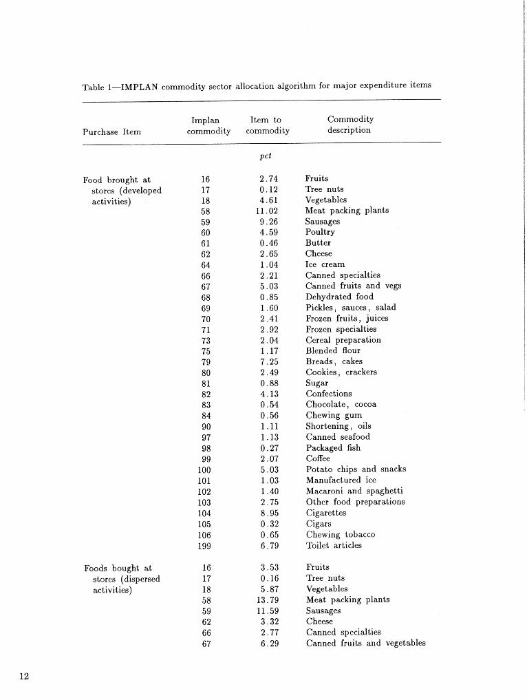
Table 1-IMPLAN commodity sector allocation algorithm for major expenditure items

Ilnplan Item to Commodity Purchase Item commodity commodity description

Food brought at 16 stores (developed 17 activities) 18

58 59 60 61 62 64 66 67 68 69 70 71 7 3 75 79 8 0 81 82 83 84 90 97 98 99

100 101 102 103 104 105 106 199

Foods bought at 16 stores (dispersed 17 activities) 18

58 5 9 6 2 66 67

Fruits Tree nuts Vegetables Meat packing plants Sausages Poultry Butter Cheese Ice cream Canned specialties Canned fruits and vegs Dehydrated food Pickles, sauces, salad Frozen fruits, juices Frozen specialties Cereal preparation Blended flour Breads, cakes Cookies, crackers Sugar Confections Chocolate, cocoa Chewing gum Shortening , oils Canned seafood Packaged fish Coffee Potato chips and snacks Manufactured ice Macaroni and spaghetti Other food preparations Cigarettes Cigars Chewing tobacco Toilet articles

Fruits Tree nuts Vegetables Meat packing plants Sausages Cheese Canned specialties Canned fruits and vegetables

Table 1-IMPLAN co dity sector allocation algorithm for major expenditure i t e m f continued)

Imp1 an Item to Commodity Purchase item commodity commodity description

Dehydrated food Pickles, sauces, salad Cereal preparation Blended flour Breads, cakes Cookies , crackers Sugar Chocolate, cocoa Chewing gum Canned seafood Coffee Potato chips and snacks Macaroni and spaghetti Cigarettes Cigars Chewing tobacco Toilet articles

Beverages bought at stores (developed activities)

Fluid milk Frozen fruits , juices Malt liquors Wine, brandy, etc. Distilled liquors Soft drinks

Beverages bought at stores (dispersed activities)

Malt liquors Wine, brandy, etc. Distilled liquors Soft drinks

Food bought at restaurantslbars

Eatingldrinking places

Gasoline and oil Refined petroleum Lubricating oils

Airfares Air transportation

Car rentals Auto rental/leasing

Other transport. Interurban passenger

Table 1-IMPLAN commodity sector allocation algorithm for major expenditure i t e m (continued)

Implan Item to Comniodity Purchase item commodity commodity description

Transportation 439 20.19 Travel agents

Lodging, private sector 463 100.00 Hotels/lodging places

Lodging, public sector

Clothing

Footwear

Do not include

111 2.27 Hosiery 124 96.47 Apparel from cloth 225 0.45 Leather gloves 228 0.82 Personal leather goods

216 21.54 Rubber/plastic footwear 224 78.46 Shoes, except rubber

Recreation equip. 473 2.81 Equipment leasing rental 488 97.19 Amusement/rec . services

Live bait services 2 6 100.00 Agriculture/forestry /fish

Prepared bait 98 100.00 Packaged fish

Fishing tackle 42 1 100.00 Sporting and athletic goods

Hunting/fishing 24 0.52 Forestrylfishery products permits 489 67.19 Membership sports / rec clubs

512 32.29 Statellocal government

Ammunition 297 100.00 Small arms ammunition

Film 413 100.00 Photographic supplies

Film developing 47 1 100.00 Commercial photofinishing

Outfitter and guide Amusement /recreation services 488 100.00 services

Table 2-Anticipated increases in recreation visitation by lake, for each water-level management alternative, low (I,), middle (M), and high (H)

Management alternative

1 2 3

Lake L M B L M H L M H

Chatuge 13.8 23.2 32.5 21.8 56.2 90.6 25.6 76.9 128.1 Fontana 22.5 37.8 53.1 52.5 69.8 87.1 82.5 150.7 218.8 I1 i wassee 8 . 4 47.4 86 .3 24.1 68.6 113.1 52.4 102.5 152.5 Santeetlah 10.6 19.1 27.5 43.6 46.8 50.0 60.6 64.7 68.8

Table 3-Anticipated increases in nonresident visitation by lake and water level management alternative, middle estimate (1,000 visits)

-

Management alternatives

Current Lake/user type (baseline) 1

Chatuge: Day boater Overnight boater Day nonboater Overnight nonboater

Fontana: Day boater Overnight boater Day nonboater Overnight nonboater

Hi wassee: Day boater Overnight boater Day nonboater Overnight nonboater

Santeetlah: Day boater Overnight boater Day nonboater Overnight nonboater

Table 4-Direct spending by nonresidents within the six-county impact region, mean per person per trip

Expenditure category

?'ram- Equip- Lakeluser type ( N ) Lodging Food portation Activity Other ment Total

Chatuge: Day nonboater Day boater Overnight nonboater Overnight boater

Fontana: Day nonboater Day boater Overnight nonboater Overnight boater

Hi wassee: Day users1 Overnight nonboater Overnight boater

Santeetlah: Day users1 Overnight nonboater Overnight boater

Boaters and nonboaters a t these lakes could not be separated because of a lirriited number of observations.

Table 5-Annual changes in economic indicators of total gross output, total income, and employment due to increases of 1,000 nonlocal recreational visits to western Narth Carolina reservoirs, six-county local impact area

Reservoir/ user type

Tot a1 industrial Tot a1

output income Employment

Chatuge: Day nonboater Day boater Overnight nonboater Overnight boater

Fontana: Day nonboater Day boater Overnight nonboater Overnight boater

IJiwassee: Day user Overnight nonboater Overnight boater

Santeetlah: Day user Overnight nonboater Overriight boater

Thozlsands of 1990 dollars Number

0 . 1 0 .6 2 . 2 1 . 4

1 .o 0 .5 3 . 5 2 . 3

0 . 3 0 .9 1 . 5

0 . 0 0 .0 0 .0

Table 6-Total economic changes for six-county area by reservoir and management alternative

Reservoir/ management alternative

Tot a1 industrial Total

output income Employment

Chatuge: Alternative 1 Alternative 2 Alternative 3

Fontana: Alternative 1 Alternative 2 Alterrlative 3

Hiwassee: Alternative 1 Alternative 2 Alternative 3

Santeetlah: Alternative 1 Alternative 2 Alterllative 3

Thousands of dollars

Table 7-Annual visitation regression model parameter estimates for Shasta Lake

Variable1 Coefficient t-stat Prob >t Elasticity

Constant -458.3800 -5.4240 0.000 -- Ln (year) 55.9490 5.0911 0.000 55.9470 Ln (May level) 6.0427 9.7098 0.000 6.0427 Ln (recdrop) -0.1684 -2.4756 0.022 -0.1684 rho 0.3044 1.4293 0.168 --

I Ln (annual recreation visitor days/1,000)-n = 20, R2 = .9055, Adj R2 = .8877, S2 = 0.010895-corrected for first-order auto correlation with Cochran-Orcutt iterative least squares procedure (Greene 1990, p. 443).

Table 8-Estimated mean annual visitation a t Shasta Lake under drought and nondrought conditions and alternative management scenarios

Condition Recreation

visitor days1

Drought baseline Drought alternative 1 Drought alternative 2

Nondrought baseline Nondrought alternative 1 Nondrought alternative 2

Corrected for log bias using the "naive factor," exp(s2/2) (Flewelling and Pienaar 1981, p. 285).

Table 9-Annual visitation regression model parameter estimates for Trinity Lake

Variable1 Coefficient t-stat Prob >t Elasticity

Const ant -437.86000 -5 .3927 0.000 -- Ln (year) 49.58800 5 .I520 0.000 49.58800 Ln (June level) 8.67780 3.3100 0.001 8.67780 Ln (Recdrop) -0.02185 -0.5588 0.582 -0.02185 Dumdat 0.58508 7 '4367 0.000 -- rho1 0.40172 2.1056 0.048 -- rho2 -0.35555 -1.8636 0.076 --

I Ln (Annual recreation visitor days/1,000)-n = 24, R2 = 3661, Adj R2 = 3380, S2 = 0.0 18823-Corrected for second-order auto correlation with Cochran-Orcutt iterative least squares procedure (Greene 1990, p. 447).

Table 10-Estimated mean annual visitation at Trinity Lake under drought and nondrought conditions and alternative management scenarios

Condition Recreation

visitor days1

Drought baseline Drought alternative 1 Drought alternative 2

Nondrought baseline Nondrought alternative 1 Nondrought alternative 2

Corrected for log bias using the "naive factor," exp(s2/2) (Flewelling and Pienaar 1981, p. 285).

Table 11-Average nonresident per trip expenditures in Sbasta and Trinity Counties, by lake and user type

Expenditure category

Lakeluser type Lodging Food Transportation Activities Other Equipment

Shasta Lake: Developed camping Dispersed camping Fishing Houseboating Other boating

Trinity Lake: Developed camping Dispersed camping Houseboating Other boating Scenic driving

Table 12-IMPLAN total economic impacts per 1,000 visits to Shasta Lake by user type

Economic impact

Activity Final Total Personal Value

demand output income added Employment l

- - - - - - - Milla'ons of 1990 dollars - - - - - - - Number

Houseboating 0.1736 0.2118 0.1222 0.1448 4.9 Other boating 0.2261 0.2723 0.1586 0.1911 6 . 1 Developed camping 0 . 1 182 0.1455 0.0810 0.0952 3 .4 Dispersed camping 0.093 1 0.1134 0.0657 0.0775 2 .8 Fishing 0.0693 0.0847 0.0479 0.0569 2 . 1

Reported in full-time job equivalents per 1,000 visits.

21

Table 13-IMPLAN total economic impacts per 1,000 visits to Shasta Lake by user type

Economic impact

Activity Final Tot a1 Personal Value

demand output income added Employment

Houseboating Other boating Developed camping Scenic driving Fishing

- - - - - - - Millions of 1990 dollars - - - - - - - - fimber

Reported in full-time job equivalents per 1,000 visits.

Table 14-Expert panel predicted activity percentages for Shasta Lake and Trinity Lake

Activity

Condition House- 0 ther Developed Dispersed Scenic boat boat camping camping driving Fishing

Shasta drought 3 3 27 10 10 -- 2 0 Shasta nondrought 3 5 27 12 10 -- 16

Trinity drought 2 1 2 5 18 -- 10 27 Trinity nondrought 20 26 31 -- 5 18

Table f 5-Total. economic impacts of recreation spending at Shasta Lake under alternative water-level management and natural conditions

Economic impact;

Final Total Personal Value Employ- Condition demand output income added ment

- . . . - e m - - Milfzolas of f 990 dollars - - - - - - - Nvmber

Drought baseline 19.84 24.09 13.89 16.56 553.1 Drought alternative 1 20.65 25.10 14.47 17.25 576.1 Drought alternative 2 21.80 26.48 15.27 18.20 607.9

Hondrought baseline 36.85 44.77 25.81 30.76 1026.9 Nondrought alternative 1 41.17 50.02 28.84 34 . 37 1147.3 Nondrought alternative 2 46.27 56.21 32.41 38.63 1289.4

Reported in full-time job equivalents.

Table 16-Total economic impacts of recreation spending at Trinity Lake under alternative water-level management and natural conditions

Economic impact

Final Tot a1 Personal Value Employ- Condition demand output income added mentl

- - - - - - - - - Millions of 1990 dollars - - - - - - - - - Number

Drought baseline 5.77 7.08 4.00 4.72 168.3 Drought alternative 1 5.81 7.13 4.02 4.75 169.5 Drought alternative 2 5.86 7.18 4.05 4.79 170.7

Nondrought baseline 7.91 9.71 5.47 6.45 231.3 Nondrought alternative 1 8.03 9.86 5.55 6.55 234.8 Nondrought alternative 2 8.16 10.01 5.64 6.65 238.4

Reported in full-time job equivalents.

23

Table 17-Combined total economic impacts of recreation spending a t Shasta Lake and 2 i n i t y Lake under alternative water-level management and natural conditions

Economic impact

Condition Final Tot a1 Personal Value Employ-

demand output income added merit1

- - - - - - - - - Millions of 1990 dollars - - - - - - - - - Nvm ber

Drought baseline 25.61 31.17 17.89 21.28 721.4 Drought alternatives 1 26.47 32.22 18.49 22.00 745.6 Drought alternatives 2 27.66 33.66 19.32 22.99 778.6

Nondrought baseline 44.73 54.48 31.28 37.22 1258.2 Nondrought alternatives 1 49.21 59.88 34.39 40.92 1382.1 Nondrought alternatives 2 54.43 66.22 38.05 45.29 1527.7

Reported in full-time job equivalents.

Table 18-Changes in tot a1 economic output (percentage deviation from baseline) for Shasta Lake and Trinity Lake under alternative water-level management and natural conditions

Indexed economic impact

Condition Shasta Trinity Weighted

Lake Lake aggregate

Drought baseline Drought aIternative 1 Drought alternative 2

- - - - - - - - Percent - - - - - - - -

Nondrought baseline 0 .0 0 .0 0 .0 Nondrought alternative 1 11.7 1 . 5 10.1 Nondrought alternative 2 25.6 3 . 1 22.0

English, B.K. Donald; Bowker, J.M.; Bergstrom, John C.; Cordell ' English, B.K. Donald; Bowker, J.M.; Bergstrom, John C.; Cordell I I H. Ken. 1995. Estimating the economic impacts of recreation response to I H. Ken. 1995. Estimating the economic impacts of recreation response to I I resource management alternatives. Gen. Tech. Rep. SIC-91. Asheville, N.C: U.S. I resource management alternatives. Gen. Tech. Rep. SC91. Asheville, N.C: U.S. I 1 Department of Agriculture, Forest Service, Southern Research Station. 24 p. I Department of Agriculture, Forest Service, Southern Research Station. 24 p. I P I I I Managing forest resources involves tradeoffs and making decisions among resource ( 1 management alternatives. Some alternatives will lead to changes in the level of 1 I recreation visitation and the amount of associated visitor spending. Thus, the

alternatives can affect local economies. This paper reports a method that can be I used to estimate the economic impacts of such alternatives. Methods for deriving 1

I representative final demand vectors and for estimating visitation response to 1 I management alternatives are presented. These methods are illustrated in two I I empirical examples that involve delaying water-level drawdown at mountain I I reservoirs. One example is for four reservoirs in western North Carolina; the other is I I for two reservoirs in northern California. 1 I

Managing forest resources involves tradeoffs and making decisions among resource I management alternatives. Some alternatives will lead to changes in the level of f recreation visitation and the amount of associated visitor spending. Thus, the alternatives can affect local economies. This paper reports a method that can be

1 used to estimate the economic impacts of such alternatives. Methods for deriving

I representative final demand vectors and for estimating visitation response to I management alternatives are presented. These methods are illustrated in two empirical examples that involve delaying water-level drawdown at mountain

I 1

reservoirs. One example is for four reservoirs in western North Carolina; the other is I for two reservoirs in northern California. 1

I t Keywords: Economic impact, recreation, reservoir level, resource management. I Keywords: Economic impact, recreation, reservoir level, resource management.

I I

The Forest Service, U.S. Department of Agriculture, is dedicated to the principle of multiple use management of the Nation's

forest resources for sustained yields of wood, water, forage, wildlife, and recreation. Through forestry research, cooperation with the States and private forest owners, and management of the National Forests and National Grasslands, i t strives-as directed by Congress-to provide increasingly greater service to a growing Nation.

The United States Department of Agriculture (USDA) Forest Service is a diverse organization committed to equal opportunity in employment and program delivery. USDA prohibits discrimination on the basis of race, color, national origin, sex, religion, age, disability, political affiliation and familial status. Persons believing they have been discriminated against should contact the Secretary, U.S. Department of Agriculture, Washington, DC 20250, or call 202-720-7327 (voice), or 202-720-1 127 (TDD).