estimating the efficiency of backtrack programs* · pdf fileestimating the efficiency of...

MATHEMATICS OF COMPUTATION, VOLUME 29, NUMBER 129

JANUARY 1975, PAGES 121-136

Estimating the Efficiency of Backtrack Programs*

By Donald E. Knuth

To Derrick H. Lehmer on his 10th birthday, February 23, 1975

Abstract. One of the chief difficulties associated with the so-called backtracking tech-

nique for combinatorial problems has been our inability to predict the efficiency of a

given algorithm, or to compare the efficiencies of different approaches, without actu-

ally writing and running the programs. This paper presents a simple method which pro-

duces reasonable estimates for most applications, requiring only a modest amount of

hand calculation. The method should prove to be of considerable utility in connection

with D. H. Lehmer's branch-and-bound approach to combinatorial optimization.

The majority of all combinatorial computing applications can apparently be han-

dled only by what amounts to an exhaustive search through all possibilities. Such

searches can readily be performed by using a well-known "depth-first" procedure which

R. J. Walker [21] has aptly called backtracking. (See Lehmer [16], Golomb and

Baumert [6], and Wells [22] for general discussions of this technique, together with

numerous interesting examples.)

Sometimes a backtrack program will run to completion in less than a second,

while other applications seem to go on forever. The author once waited all night for

the output from such a program, only to discover that the answers would not be forth-

coming for about 106 centuries. A "slight increase" in one of the parameters of a

backtrack routine might slow down the total running time by a factor of a thousand;

conversely, a "minor improvement" to the algorithm might cause a hundredfold im-

provement in speed; and a sophisticated "major improvement" might actually make

the program ten times slower. These great discrepancies in execution time are charac-

teristic of backtrack programs, yet it is usually not obvious what will happen until the

algorithm has been coded and run on a machine.

Faced with these uncertainties, the author worked out a simple estimation pro-

cedure in 1962, designed to predict backtrack behavior in any given situation. This

procedure was mentioned briefly in a survey article a few years later [8] ; and during

subsequent years, extensive computer experimentation has confirmed its utility. Several

Received July 12, 1974.

AMS (MOS) subject classifications (1970). Primary 68A20, 05-04; Secondary 05A15,

65C05, 90B99.

Key words and phrases. Backtrack, analysis of algorithms, Monte Carlo method, Instant In-

sanity, color cubes, knight's tours, tree functions, branch and bound.

* This research was supported in part by the Office of Naval Research under contract

NR 044-402 and by the National Science Foundation under grant number GJ 36473X. Reproduc-

tion in whole or in part is permitted for any purpose of the United States Government.

Copyright © 1975. American Mathematical Society

121

License or copyright restrictions may apply to redistribution; see http://www.ams.org/journal-terms-of-use

122 DONALD E. KNUTH

improvements on the original idea have also been developed during the last decade.

The estimation procedure we shall discuss is completely unsophisticated, and it

probably has been used without fanfare by many people. Yet the idea works surpris-

ingly well in practice, and some of its properties are not immediately obvious, hence

the present paper might prove to be useful.

Section 1 presents a simple example problem, and Section 2 formulates back-

tracking in general, developing a convenient notational framework; this treatment is

essentially self-contained, assuming no prior knowledge of the backtrack literature. Sec-

tion 3 presents the estimation procedure in its simplest form, together with some theo-

rems that describe the virtues of the method. Section 4 takes the opposite approach,

by pointing out a number of flaws and things that can go wrong. Refinements of the

original method, intended to counteract these difficulties, are presented in Section 5.

Some computational experiments are recorded in Section 6, and Section 7 summarizes

the practical experience obtained with the method to date.

1. Introduction to Backtrack. It is convenient to introduce the ideas of this pa-

per by looking first at a small example. The problem we shall study is actually a rath-

er frivolous puzzle, so it does not display the economic benefits of backtracking; but

it does have the virtue of simplicity, since the complete solution can be displayed in a

small diagram. Furthermore the puzzle itself seems to have been tantalizing people for

at least sixty years (see [19]); it became extremely popular in the U.S.A. about 1967

under the name Instant Insanity.

Figure 1 shows four cubes whose faces are colored red (R), white (W), green (G),

or blue (B); colors on the hidden faces are shown at the sides. The problem is to ar-

range the cubes in such a way that each of the four colors appears exactly once on

the four back faces, once on the top, once in the front, and once on the bottom.

Thus Figure 1 is not a solution, since there is no blue on the top nor white on the

bottom; but a solution is obtained by rotating each cube 90°.

Cube 1 Cube 2 Cube 3 Cube h

Figure 1. Instant Insanity cubes

We can assume that these four cubes retain their relative left-to-right order in all

solutions. Each of the six faces of a given cube can be on the bottom, and there are

four essentially different positions having a given bottom face, so each cube can be

placed in 24 different ways; therefore the "brute force" approach to tjjris problem is to


ESTIMATING THE EFFICIENCY OF BACKTRACK PROGRAMS 123

try all of the 244 = 331776 possible configurations. If done by hand, the brute force

procedure might indeed lead to insanity, although not instantly.

It is not difficult to improve on the brute force approach by considering the ef-

fects of symmetry. Any solution clearly leads to seven other solutions, by simulta-

neously rotating the cubes about a horizontal axis parallel to the dotted line in Figure 1,

and/or by rotating each cube 180° about a vertical axis. Therefore we can assume with-

out loss of generality that Cube 1 is in one of three positions, instead of considering all

24 possibilities. Furthermore it turns out that Cube 2 has only 16 essentially different

placements, since it has two opposite red faces; see Figure 2, which shows that two of

its 24 positionings have the same colors on the front, top, back, and bottom faces. The

same observation applies to Cube 3. Hence the total number of essentially different

ways to position the four cubes is only 3 • 16 • 16 • 24 = 18432; this is substantially

less than 331776, but it might still induce insanity.

Cube 2 Cube 2

/SB

1/

Figure 2. Rotation by 180° in this case leaves the relevant colors unchanged

A natural way to reduce the number of cases still further now suggests itself.

Given one of the three placements for Cube 1, some of the 16 positionings of Cube 2

are obviously foolhardy since they cannot possibly lead to a solution. In Figure 1, for

example, Cubes 1 and 2 both contain red on their bottom face, while a complete solu-

tion has no repeated colors on the bottom, nor on the front, top, or back; since this

placement of Cube 2 is incompatible with the given position of Cube 1, we need not

consider any of the 16 • 24 = 384 ways to place Cubes 3 and 4. Similarly, when

Cubes 1 and 2 have been given a compatible placement, it makes sense to place Cube

3 so as to avoid duplicate colors on the relevant sides, before we even begin to con-

sider Cube 4.

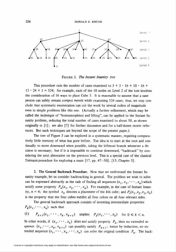
Such a sequential placement can be represented by a tree structure, as shown in

Figure 3. The three nodes just below the root (top) of this tree stand for the three es-

sentially different ways to place Cube 1. Below each such node are further nodes rep-

resenting the possible placements of Cube 2 in a compatible position; and below the

latter are the compatible placements of Cube 3 (if any), etc. Note that there is only

one solution to the puzzle, represented by the single node on Level 4.


124 DONALD E. KNUTH

l -¡_ Level h

Figure 3. The Instant Insanity tree

This procedure cuts the number of cases examined to 3 + 3 • 16 4- 10 • 16 4-

13 • 24 + 1 = 524; for example, each of the 10 nodes on Level 2 of the tree involves

the consideration of 16 ways to place Cube 3. It is reasonable to assume that a sane

person can safely remain compos mentis while examining 524 cases; thus, we may con-

clude that systematic enumeration can cut the work by several orders of magnitude

even in simple problems like this one. (Actually a further refinement, which may be

called the technique of "homomorphism and lifting", can be applied to the Instant In-

sanity problem, reducing the total number of cases examined to about 50, as shown

originally in [1] ; see also [7] for further discussion and for a half-dozen recent refer-

ences. But such techniques are beyond the scope of the present paper.)

The tree of Figure 3 can be explored in a systematic manner, requiring compara-

tively little memory of what has gone before. The idea is to start at the root and con-

tinually to move downward when possible, taking the leftmost branch whenever a de-

cision is necessary; but if it is impossible to continue downward, "backtrack" by con-

sidering the next alternative on the previous level. This is a special case of the classical

Trémauxprocedure for exploring a maze [17, pp. 47—50], [13, Chapter 3].

2. The General Backtrack Procedure. Now that we understand the Instant In-

sanity example, let us consider backtracking in general. The problem we wish to solve

can be expressed abstractly as the task of finding all sequences (xltx2,m • ■ , xn) which

satisfy some property Pn{x., x2, • • • , xn). For example, in the case of Instant Insan-

ity, n = 4; the symbol xk denotes a placement of the kth cube; and Pr(x.,x2,x3,x4)

is the property that the four cubes exhibit all four colors on all four relevant sides.

The general backtrack approach consists of inventing intermediate properties

Pk{x-,, • • • , xk) such that

A) pk+i{xi> ' ' ' > xk> xk+i) implies Pkix,,• • • , xk) for 0 < k < n.

In other words, if {x., • • • , xk) does not satisfy property Pk, then no extended se-

quence (jtj,* • • ,xk, xk+l) can possibly satisfy Pk+1 ; hence by induction, no ex-

tended sequence (x1, • • • , xk, • • •, x ) can solve the original condition P The back-



track procedure systematically enumerates all solutions {x., • • • , xn) to the original

problem by considering all partial solutions {x¡, • • • , xk) that satisfy Pk, using the

following general algorithm:

Step Bl. [Initialize.] Set k to 0.

Step B2. [Compute the successors.] (Now Pk{x., • • •, xk) holds, and 0 < k

< «.) Set Sk to the set of all xk+. suchthat Pk+i{xl,' ' ', xk, xk+1) is true.

Step B3. [Have all successors been tried?] If Sk is empty, go to Step B6.

Step B4. [Advance.] Choose any element of Sk, call it xk+1, and delete it

from Sk. Increase k by 1.

Step B5. [Solution found?] (Now Pk(x. ,-•• ,xk) holds, and 0 < k < «.)

If k <n, return to Step B2. Otherwise output the solution {xl,m • • ,xn) and go on to

Step B6.

Step B6. [Backtrack.] (All extensions of (xt, ■ ■ • , xk) have now been ex-

plored.) Decrease k by 1. If k > 0, return to Step B3; otherwise the algorithm

terminates. D

Condition (1) does not uniquely define the intermediate properties Pk, so we

often have considerable latitude when we choose them. For example, we could simply

let Pk be true for all {x., • • • , xk), when k < n; this is the weakest possible prop-

erty satisfying (1), and it corresponds to the brute force approach, where some 244

possibilities would be examined in the cube problem. On the other hand the strongest

property is obtained when Pk{xl, • • •, xk) is true if and only if there exist xk+1,

• • •, xn satisfying Pn{xl,' ' ', xk, xk+ ,,••', xn). In our example this strongest

property would reduce the search to the examination of a trivial twig of a tree, but the

decisions at each node would require considerable calculation. In general, stronger

properties limit the search but require more computation, so we want to find a suit-

able trade-off. The solution adopted in our example (namely to use symmetry consid-

erations when placing Cubes 1, 2, and 3, and to let Pk{xl, • ■ •, xk) mean that no

colors are duplicated on the four relevant sides) is fairly obvious, but in other problems

the choice of Pk is not always so self-evident.

3. A Simple Estimate of the Running Time. For each {x., • • • , xk) satisfying

Pk with 0 < k < n, the algorithm of Section 2 will execute Steps B2, B4, B5, and B6

once, and Step B3 twice. (To see this, note that it is true for Steps B2, B5, and B6,

and apply Kirchhoffs law as in [12].) Let us call the associated running time the cost

c{x., • • •, xk). When k = n, the corresponding cost amounts to one execution of

Steps B3, B4, B5, and B6. If we also let c( ) be the cost for k = 0 (i.e., one

execution of Steps Bl, B2, B3, and B6), the total running time of the algorithm comes

to exactly

(2) Z S c(*i. ••*.*»)■k>o Pk{xv-,xk)

This formula essentially distributes the total cost among the various nodes of the


126 DONALD E. KNUTH

tree. Since the time to execute Step B2 can vary from node to node, and since the time

to execute Step B5 depends on whether or not k = n, the running time is not simply

proportional to the size of the tree except in simple cases.

Let T be the tree of all possibilities explored by the backtrack method; i.e.,let

(3) T = {(*!,•• ', xk)\k> 0 and Pk(Xl, • • • , xk) holds}.

Then we can rewrite (2) as

(4) cost (7) = Z <*f).tGT

Our goal is to find some way of estimating cost(7), without knowing a great deal

about the properties Pk, since the example of Section 1 indicates that these proper-

ties might be very complex.

A natural solution to this estimation problem is to try a Monte Carlo approach,

based on a random exploration of the tree; for each partial solution (Xj, • • • , xk)

for 0 < k < «, we can choose xk+. at random from among the set Sk of all con-

tinuations, as in the following algorithm. (A related procedure, but which is intrin-

sically different because it is oriented to different kinds of estimates, has been pub-

lished by Hammersley and Morton [10], and it has been the subject of numerous pa-

pers in the literature of mathematical physics; see [5].)

Step El. [Initialize.] Set k <— 0, D <— 1, and C+-c{). (Here C will be

an estimate of (2), and D is an auxiliary variable used in the calculation of C,

namely the product of all "degrees" encountered in the tree. An arrow " *— " de-

notes the assignment operation equivalent to Algol's " := "; and c{ ) denotes the

cost at the root of the tree, as in (2) when k = 0.)

Step E2. [Compute the successors.] Set Sk to the set of all xk+l suchthat

Pk+. (Xj, • • • , xk, xk+l) is true, and let dk be the number of elements of Sk.

(If k = «, then Sk is empty and dk = 0.)

Step E3. [Terminal position?] If dk = 0, the algorithm terminates, with C

an estimate of cost (7).

Step E4. [Advance.] Choose an element xk+l€.Sk at random, each element

being equally likely. (Thus, each choice occurs with probability l/dk.) Set D <—

dkD, then set C «—C + c{xl,- • •,xk+1)D. Increase k by 1 and return to

Step E2. D

This algorithm makes a random walk in the tree, without any backtracking, and

computes the estimate

(5) C = c{) + dr.cix^ + d0d,c{xx, x2) + d0dld2c{x1, x2, x3) + • • • ,

where dk is a function of {xt,'' ' , xk), namely the number of xk+l satisfying

Pk+1{xi, • • • , xk, xk+l). We may define dk = 0 for all large k, thereby regarding

(5) as an infinite series although only finitely many terms are nonzero.

The validity of estimate (5) can be proved as follows.



Theorem 1. The expected value of C, as computed by the above algorithm, is

cost (7), as defined in (4).

Proof. We shall consider two proofs, at least one of which should be convinc-

ing. First we can observe that for every t = (JCj, • • •, xk) G T, the term

(6) d0d. • • ' dk_.c{xl,- • • ,xk)

occurs in (5) with probability l/d0di ■ • • dk_l, since this is the chance that the al-

gorithm will consider the partial solution (Xj, • • • xk). Hence the sum of all the terms

(6) has the expected value (4).

The second proof is based on a recursive definition of cost (T), namely

(7) cost {T) = c{) + cost (7\) + • • • + cost {Td),

where d = d0 is the degree of the root of the tree and T., • • • , Td are the respec-

tive subtrees of the root, namely

Tj = {(*!,•••, xk) € T IJC, is the /th element of S0}.

We also have C = c( ) + d0C', where C' = c{x¡) + d.cixx, x2) + d.d2cix., x2, x3)

+ • • ' has the form of (5) and is an estimate of one of the T-. Since each of the

d = dQ values of / is equally likely, the expected value of C is

E{C) = c{) + d0E{C) = c{) + d^iEÍC,) + • • • + E{Cd))/d),

where E{C) = cost (7p by induction on the size of the tree. Hence E{C) =

cost (7). D

This theorem demonstrates that C is indeed an appropriate statistic to compute,

based on one random walk down the tree. As an example of the theorem, let us con-

sider Figure 3 in Section 1, using the costs shown there (since they represent the time

to perform Step B2, which dominates the calculation). We have cost (7) = 524, and

if the estimation algorithm is applied to the tree it is not difficult to determine that

the result will be C = 243, or 291, or 435, or 531, or 543, or 819, or 1107, with

respective probabilities 1/6, 1/6, 1/6, 1/6, 1/12, 1/6, and 1/12. Thus, a fairly reason-

able approximation will nearly always be obtained; and we know that the mean of

repeated estimates will approach 524, by the law of large numbers.

Since the proof of Theorem 1 applies to all functions c{t) defined over trees,

we can apply it to other functions in order to obtain further information:

Corollary 1. The expected value of D at the end of the above algorithm is

the number of terminal nodes in the tree.

Proof. Let c(i) =1 if í is terminal, and c{t) = 0 otherwise; then C =

D at the end of the algorithm, hence E{D) = E{C) = H)c{t) is the number of terminal

nodes by Theorem 1. D

Corollary 2. The expected value of the product d0d. • • 'dk_. for fixed k,


128 DONALD E.KNUTH

when the d-'s are computed by the above algorithm, is the number of nodes on level

k of the tree.

Proof. Let c{t) = 1 for all nodes on level k, and c{t) = 0 otherwise; then

C = d0d. *k-i at the end of the algorithm. (Note that d0d. dk_. is zero

if the algorithm terminates before reaching level k.) O

Corollary 2 gives some insight into the "meaning" of the individual terms of our

estimate (5); the term d0dl c{x., • • • , xk) represents the number of

nodes on level k times the cost associated with a typical one of these nodes.

4. Some Cautionary Remarks. The algorithm of Section 3 seems too simple to

work, and there are many intuitive grounds for skepticism, since we are trying to pre-

dict the characteristics of an entire tree based on the knowledge of only one branch!

The combinatorial realities of most backtrack applications make it clear that different

partial solutions can have drastically different behavior'patterns.

Just knowing that an experiment yields the right expected value is not much con-

solation in practice. For example, consider an experiment which produces a result of

1 with probability 0.999, while the result is 1,000,001 with probability 0.001; the

expected value is 1001, but a limited sampling would almost always convince us that

the true answer is 1.

There is reason to suspect that the estimation procedure of Section 3 will suffer

from precisely this defect: It has the potential to produce huge values, but with very

low probability, so that the expected value might be quite different from typical esti-

mates.

Let Nk be the number of nodes on level k of the tree (cf. Corollary 2). In

most backtrack applications, the vast majority of all nodes in the search tree are con-

centrated at only a few levels, so that in fact the logarithm of Nk (the number of

digits in A^fc) has a bell-shaped curve when plotted as a function of k:

(8)log N,

On the other hand our estimate (5) is composed of a series of estimates N'k = d0d1

• • • dk_. which are never bell-shaped; since the d's are integers, the N'k grow ex-

ponentially with k, until finally dropping to zero:

(9)log N' LA

Although these two graphs have completely different characteristics, we are getting es-



timates which in the long run produce (8) as an average of curves like (9).

Consider also Figure 3, where we have somewhat arbitrarily assigned a cost of 1

to the lone solution node on Level 4. Perhaps our output routine is so slow that the

solution node should really have a cost of 106; this now becomes the dominant por-

tion of the total cost, but it will be considered only 1/12 of the time, and then it will

be multiplied by 12.

There is clearly a danger that our estimates will almost always be low, except for

rare occasions when they will be much too high.

5. Refinements. Our estimation procedure can be modified in order to circum-

vent the difficulties sketched in Section 4. One idea is to introduce systematic bias

into Step E4, so that the choice of xk+l is not completely random; we can try to

investigate the more interesting or more difficult parts of the tree.

The algorithm can be generalized by using the following selection procedure in

place of Step E4.

Step E4'. [Generalized advance.] Determine, in any arbitrary fashion, a sequence

of dk positive numbers Pk{l), Pk{2), • • •, Pk{dk) whose sum is unity. Then choose

a random integer Jk in the range 1 < Jk < dk in such a way that Jk = / with

probability pk(f). Let xk+1 be the Jkth element of Sk, and set D<—D/pk{Jk),

C+—C + c(x1,' • • , xk+i)D. Increase k by 1 and return to Step E2. D

(Step E4 is the special case pk(j) = 1 ¡dk for all /.) Again we can prove that

the expected value of C will be cost (7), no matter how strangely the probabilities

pk(j) are biased in Step E4'; in fact, both proofs of Theorem 1 are readily extended

to yield this result. It is interesting to note that the calculation of D involves a pos-

teriori probabilities, so that it grows only slightly after a highly probable choice has

been made. The technique embodied in Step E4' is generally known as importance

sampling [9, pp. 57-59].

Some choices of the pk(J) are much better than others, of course, and the most

interesting fact is that one'of the possible choices is actually perfect:

Theorem 2. If the probabilities pkij) in Step E4' are chosen appropriately, the

estimate C will always be exactly equal to cost (7).

Proof. For 1 </' <dk, let pk(j) be

costjTjx.,- • • ,xk,xk+1(J)))

{ ' Pfc(/) cost(7(x1, • • • , xk)) - c(xlt • • • , xk)'

where T{xx, • • • , xk) is the set of all t £ 7 having specified values {x¡, • • • , xk)

for the first k components, and where xk+l(j) is the /th element of Sk. Now we

can prove that the relation

C + (costil, • • • , xk)) - c{x., • • • , xk))D = cost(7)

is invariant, in the sense that it always holds at the beginning and end of Step E4'.


130 DONALD E.KNUTH

Since cost {T{x., • • • , xk)) = c{x.,• • •, xk) when dk = 0, the algorithm terminates

with C = cost (7).

Alternatively, using the notation in the second proof of Theorem 1, we have

C = c{) + ((cost (7) - c{ ))/cost{Tj))Cj

for some /, and C¡ = cost(7;) by induction, hence C=cost(7). D

Of course we generally need to know the cost of the tree before we know the

exact values of these ideal probabilities Pk(j), so we cannot achieve zero variance in

practice. But the form of the p|(/) shows what kind of bias is likely to reduce the

variance; any information or hunches that we have about relative subtree costs will be

helpful. (In the case of Instant Insanity there is no simple a priori reason to prefer one

cube position over another, so this idea does not apply; perhaps Instant Insanity is a

mind-boggling puzzle for precisely this reason, since intuition is usually much more

valuable.)

Theorem 2 can be extended considerably, in fact we can derive a general formula

for the variance. The generating function for C satisfies

00 C(Z) = z<() Z PjCj{zl'Pi)

and from this equation it follows by differentiation that

var(C) = C"(l) + C(l) - C{1)2

(12) ^ ^ /cost (7,.) cost (7,) \2- £ var(C/)/P/+ Z PiPjV—^- ■-JA) -

Kj<d Ki<j<d \ Pi Pi I

Iterating this recurrence shows that the variance can be expressed as

(.3) »©-£¿5 Z P'(W^-=i«)',rerrW i<í</<</(í) \ p\i) prij) J

where Pit) is the probability that node t is encountered, d{t) is the degree of

node t, ptQ) is the probability that we go from t to its /th successor, and T{t, j)

is the subtree rooted at that successor.

From this explicit formula we can get a bound on the variance, if the probabil-

ities are reasonably good approximations to the relative subtree costs:

Theorem 3. If the probabilities pk(j) in Step EA' satisfy

cost{T{x.,- •• ,xk,xk+i(j))) cost (TÍJCp- • • , xfc, jck (;)))-—-<a- -

PfcO) Pk{i)

for all i, j and for some fixed constant a> I, the variance of C is at most

a2+2a+lY ,\ „_w.«204) ((» —-) l)cost(7f.



Proof. Let q, = cost(7)/p-, and assume without loss of generality that q. <

q2^ " ' ' ^ ad < tv^j. From elementary calculus we have, under the constraints

cost (7}) > 0 and S p. = 1,

Cost(r;.)2 a2 + 2a+1/ y

K/<d P/ qa \i</<d /

equality occurring when cf = 2 and q2-aq1. Furthermore

\2

Z PiPjtii - ijfKi<j<d

cost(7,)z / \a

Z -( Z cort(7»1</«<Í 1</<<J

Letting (3 = (a2 + 2a + l)/4a, we can prove (14) by induction since (12) now yields

var(C)< Z ™{Cj)/Pj + {ß -l)cost(T)2K/<d

< Z {ß"~l - 1)cost {T,)2/p, + (ß~l)cost (7)2K/<d

(j3" -|3)cost(7)2 + (|3 - l)cost(T)2 D

Theorem 3 implies Theorem 2 when a = 1; for a > 1 the bound in (14) is

not especially comforting, but it does indicate that a few runs of the algorithm will

probably predict cost (7) with the right order of magnitude.

Another way to improve the estimates is to transform the tree into another one

having the same total cost, and to apply the Monte Carlo procedure to the transformed

tree. For example, the tree fragment

with costs Cl, ■

aß 7 6 E £ T)

C» and subtrees a,- • • ,-q can be replaced by' ^s

C1+C2 + C3 + CVC5

a ß 7 ô e C T]

by identifying five nodes. Intermediate condensations such as


132 DONALD E. KNUTH

C, +C, + C,1 3 h

ate also possible.

One application of this idea, if the estimates are being made by a computer pro-

gram, is to eliminate all nodes on levels 1, 3, 5, 7, • • • of the original tree, making the

nodes formerly on levels 2k and 2k + 1 into a new level k. For example, Figure 4

shows the tree that results when this idea is applied to Figure 3. The estimates in this

collapsed tree are C= 211, or 451, or 461, or 691, or 931, with respective probabil-

ities .2, .3, .1, .3, .1, so we have a slightly better distribution than before.

51

61+ to 1+0 61+ 16 1+0 1+0 88 16 6U

Figure 4. Collapsed Instant Insanity tree

Another use of this idea is to eliminate all terminal nodes having nonterminal

"brothers". Then we can ensure that the algorithm never moves directly to a configu-

ration having dk = 0 unless all possible moves are to such a terminal situation ; in

other words, "stupid" moves can be avoided.

Still another improvement to the general estimation procedure can be achieved by

"stratified sampling" [9, pp. 55—57]. We can reduce the variance of a series of esti-

mates by insisting for example that each experiment chooses a different value of xt.

6. Computational Experience. The method of Section 3 has been tested on

dozens of applications; and despite the dire predictions made in Section 4 it has con-

sistently performed amazingly well, even on problems which were intended to serve as

bad examples. In virtually every case the right order of magnitude for the tree size was

found after ten trials. Three or four of the ten trials would typically be gross under-

estimates, but they were generally counterbalanced by overestimates, in the right pro-

portion.

We shall describe only the largest experiment here, since the method is of most

critical importance on a large tree. Figure 5 illustrates the problem that was considered,

the enumeration of uncrossed knight's tours; these are nonintersecting paths of a

knight on the chessboard, where the object is to find the largest possible tour of this

kind. T. R. Dawson first proposed the problem in 1930 [2], and he gave the two 35-



move solutions of Figure 5, stating that "il est probablement impossible de dénombrer

la quantité de ces tours; . . . vraisemblablement, on ne peut effectuer plus de 35 coups."

Later [3, p. 20], [4, p. 35] he stated without proof that 35 is maximum.

wt.#;ï>*i

V"-^i

Wf,tf

*f

Figure 5. Uncrossed knight's tours

The backtrack method provides a way to test his assertion; we may begin the

tour in any of 10 essentially different squares, then continue by making knight's moves

that do not cross previous ones, until reaching an impasse. But backtrack trees that

extend across 30 levels or more can be extremely large; even if we assume an average

of only 3 consistent choices at every stage, out of at most 7 possible knight moves to

new squares, we are faced with a tree of about 330 = 205,891,132,094,649 nodes,

and we would never finish. Actually 320 = 3,486,784,401 is nearer the upper limit

of feasibility, since it is not at all simple to test whether or not one move crosses

another. It is certainly not clear a priori that an exhaustive backtrack search is eco-

nomically feasible.

The simple procedure of Section 3 was therefore used to estimate the number of

nodes in the tree, using c(r) = 1 for all t. Here are the estimated tree sizes found in

the first ten independent experiments:

1571717091315291281

82311793651

59761491

20974951158736818301

311259271

6071489081

The mean value is 6,696,688,822. The next sequence of ten experiments gave the es-

timates

567911111

569585831111411

2384134916697691

5848873631161

140296511

for an average of only 680,443,586, although the four extremely low estimates make


134 DONALD E. KNUTH

this value look highly suspicious. (We could have avoided the "stupid moves" which

lead to such low estimates, by using the technique explained at the end of Section 5,

but the original method was being followed faithfully here.) After 100 experiments

had been conducted, the observed mean value of the estimates was 1,653,634,783.8,

with an observed standard deviation of about 6.7 x 109.

The first few experiments were done by hand, but then a computer program was

written and it performed 1000 experiments in about 30 seconds. The results of these

experiments were extremely encouraging, because they were able to predict the size of

the tree quite accurately as well as its "shape" (i.e., the number Nk of nodes per

level), even though the considerations of Section 4 seem to imply that Nk cannot be

estimated well. Table 1 shows how these estimates compare to the exact values which

were calculated later; there is surprisingly good agreement, although the experiment

looked at less than 0.00001 of the nodes of the tree. Perhaps this was unusually

good luck.

This knight's tour problem reflects the typical growth of backtrack trees; the

same problem on a 7x7 board generates a tree with 10,874,674 nodes and on a

6x6 board there are only 88,467. On a 9 x 9 board we need another method; the

longest known tour has 47 moves [18]. It can be shown that the longest reentrant

tour on an « x « board has at least «2 — 0{n) moves, see [11].

7. Use of the Method in Practice. There are two principal ways to apply this

estimation method, namely by hand and by machine.

Hand calculation is especially recommended as the first step when embarking on

any backtrack computations. For one thing, the algorithm is great fun to apply, es-

pecially when decimal dice [20] are used to guide the decisions. The reader is urged

to try constructing a few random uncrossed knight's tours, recording the statistics dk

as the tours materialize; it is a captivating game that can lead to hours of enjoyment

until the telephone rings.

Furthermore, the game is worthwhile, because it gives insight into the behavior of

the algorithm, and such insight is of great use later when the algorithm is eventually

programmed; good ideas about data structures, and about various improvements in the

backtracking strategy, usually suggest themselves. The assignment of nonuniform prob-

abilities as suggested in Section 5 seems to improve the quality of the estimates, and

adds interest to the game. Usually about three estimates are enough to give a feeling

for the amount of work that will be involved in a full backtrack search.

For large-scale experiments, expecially when considering the best procedure in

some family of methods involving parameters that must be selected, the estimates can

be done rapidly by machine. Experience indicates that most of the refinements sug-

gested in Section 5 are unnecessary; for example, the idea of collapsing the tree into

half as many levels does not improve the quality of the estimates sufficiently to justify

the greatly increased computation. Only the partial collapsing technique which avoids

"stupid moves" is worth the effort, and even this makes the program so much more



TABLE 1. Estimates after 1000 random walks

Estimate, Nj. True value, Nh

01

2

34

S

6

7

8

910

11

12

1314

IS

1617

18

19

2(1

21

22

2.!

24

25

26

27

28

29

30

3132

3334

35

36

1.0

10.0

42.8

255.0

991.4

4352.2

16014.4

59948.8

190528.7

580450.8

1652568.7

4424403.9

9897781.4

22047261.5

44392865.5

92464977.5

145815116.2

238608697.6

253061952.9

355460520.9

348542887.6

328849873.9

340682204.1

429508177.9

318416025.6

38610432.0

75769344.0

74317824.0

0.0

0.0

0.0

0.0

0.0

0.0

0.0

0.0

0.0

1

10

42

251

968

4215

15646

56435

182520

574555

1606422

437615310396490

23978392

47667686

91377173

150084206

235901901

315123658

399772215

427209856

429189112

358868304

278831518

177916192

103894319

49302574

21049968

7153880

2129212

S22186

109254

18862

2710

346

50

8

Total 3123375511.1 3137317290

complex that it should probably be used only when provided as a system subroutine.

(A collection of system routines or programming language features, that allow both the

estimation algorithm and full backtracking to be driven by the same source language

program, is useful.)

Perhaps the most important application of backtracking nowadays is to combina-

torial optimization problems, as first suggested by D. H. Lehmer [15, pp. 168-169].

In this case the method is commonly called a branch-and-bound technique (see [14]).

The estimation procedure of Section 3 does not apply directly to branch-and-bound al-

gorithms; however, it is possible to estimate the amount of work needed to test any

given bound for optimality. Thus we can get a good idea of the running time even in

this case, provided that we can guess a reasonable bound. Again, hand calculations

using a Monte Carlo approach are recommended as a first step in the approach to all

branch-and-bound procedures, since the random experiments provide both insight and

enjoyment.


136 DONALD E. KNUTH

Acknowledgments. I wish to thank Robert W. Floyd and George W. Soules for

several stimulating conversations relating to this research. The knight's tour calcula-

tions were performed as "background computation" during a period of several weeks,

on the computer at IDA-CRD in Princeton, New Jersey.

Computer Science Department

Stanford University

Stanford, California 94305

1. F. DE CARTEBLANCHE, "The colored cubes problem," Eureka, v. 9, 1947, pp. 9-11.

2. T. R. DAWSON, "Echecs Féeriques," problem 186, L'Echiquier, (2), v. 2, 1930, pp. 1085-

1086; solution in L'Echiquier, (2), v. 3, 1931, p. 1150.

3. T. R. DAWSON, Caissa's Wild Roses, C. M. Fox, Surrey, England, 1935; reprinted in Five

Classics of Fairy Chess, Dover, New York, 1973.

4. T. R. DAWSON, "Chess facts and figures," Chess Pie III, souvenir booklet of the Interna-

tional chess tournament, Nottingham, 1936, pp. 34—36.

5. PAUL J. GANS, "Self-avoiding random walks. I. Simple properties of intermediate-walks,"

J. Chem. Phys., v. 42, 1965, pp. 4159-4163. MR 32 #3147.

6. SOLOMON W. GOLOMB & LEONARD D. BAUMERT, "Backtrack programming," /. Assoc.

Comput. Mach., v. 12, 1965, pp. 516-524. MR 33 #3783.

7. N. T. GRIDGEMAN, "The 23 colored cubes," Math. Mag., v. 44, 1971, pp. 243-252.

8. MARSHALL HALL, JR. & D. E. KNUTH, "Combinatorial analysis and computers," .4mer.

Math. Monthly, v. 72, 1965, no. 2, part II, pp. 21-28. MR 30 #3030.

9. J. M. HAMMERSLEY & D. C. HANDSCOMB, Monte Carlo Methods, Methuen, London;

Barnes & Noble, New York, 1965. MR 36 #6114.

10. J. M. HAMMERSLEY & K. W. MORTON, "Poor man's Monte Carlo," /. Roy. Statist.

Soc. Ser. B, v. 16, 1954, pp. 23-28. MR 16, 287.

11. DONALD E. KNUTH, "Uncrossed knight's tours," (letter to the editor), J. Recreational

Math., v. 2, 1969, pp. 155-157.

12. DONALD E. KNUTH, Fundamental Algorithms, The Art of Computer Programming,

vol. 1, second edition Addison-Wesley, Reading, Mass., 1973.

13. DENES KONIG, Theorie der endlichen und unendlichen Graphen, Leipzig, 1936; reprint,

Chelsea, New York, 1950.

14. E. L. LAWLER & D. E. WOOD, "Branch-and-bound methods: A survey," Operations

Research, v. 14, 1966, pp. 699-719. MR 34 #2338.

1 5. DERRICK H. LEHMER, "Combinatorial problems with digital computers," Proc Fourth

Canadian Math. Congress (1957), Univ. of Toronto Press, Toronto, 1959, pp. 160-173. See also:

Proc. Sympos. Appl. Math., vol. 6, Amer. Math. Soc, Providence, R. I., 1956, pp. 115, 124, 201.

16. DERRICK H. LEHMER, "The machine tools of combinatorics," Chapter 1 in Applied

Combinatorial Mathematics, edited by Edwin F. Beckenbach, Wiley, New York, 1964, pp. 5—31.

17. EDOUARD LUCAS, Récréations Mathématiques, v. 1, Paris, 1882.

18. MICHIO MATSUDA & S. KOBAYASHI, "Uncrossed knight's tours," (letter to the edi-

tor), /. Recreational Math., v. 2, 1969, pp. 155-157.

19. T. H. O'BIERNE, Puzzles and Paradoxes, Oxford Univ. Press, New York and London,

1965.

20. C. B. TOMPKINS, review of "Random-number generating dice," by Japanese Standards

Association, Math. Comp., v. 15, 1961, pp. 94-95.

21. R. J. WALKER, "An enumerative technique for a class of combinatorial problems,"

Proc. Sympos. Appl. Math., vol. 10, Amer. Math. Soc, Providence, R. I., 1960, pp. 91-94. MR 22

#12048.

22. MARK B. WELLS, Elements of Combinatorial Computing, Pergamon Press, Oxford and

New York, 1971. MR 43 #2819.

23. L. D. YARBROUGH, "Uncrossed knight's tours,"/. Recreational Math., v. 1, 1968, pp.

140-142.


estimating the efficiency of backtrack programs* · pdf fileestimating the efficiency of...

Documents