estimating the precision of under-water...
TRANSCRIPT

Estimating the Precision of Under-Water Video-Mosaics
E. Michaelsen, N. Scherer-Negenborn
Fraunhofer-IOSB, Gutleuthausstrasse1,76275 Ettlingen, Germany
Abstract
Under-water video-mosaics are an important tool
e.g. for inspection of man-made infrastructure.
Cameras may drift in rotation and distance to the
surface while the mosaic will often be very much
larger than a single frame resulting in long chains of
planar homographies. This contribution addresses the
problems arising from dead-reckoning drift in such
chains. Local patches are rectified using homography
decomposition. Experiments with a portal allowing
underwater image sequences with mechanical
groundtruth are performed. Thus the deviation of the
mosaic from a true orthographic map may be
estimated.
1. Introduction
Visual Inspection of man-made underwater
infrastructure from unmanned platforms is of
increasing interest. Another application can be
mapping of the seafloor. Due to poor visibility
conditions the distance between camera and observed
surface must be kept short. Therefore, wide-angle lens
are used. Large image mosaics are stitched with the
camera moving back and forth along the surface. It is
of crucial importance to estimate the drift error
occurring in such mosaics.
2. Related work
Optimal estimation of homogenous entities, such as
planar homography matrices, with more entries than
degrees of freedom from image to image
correspondences including sound uncertainty
propagation is treated in [3]. Robust estimation using
RANSAC is state-of-the-art. There are, however,
alternatives such as GoodSAC [8], SURSAC [11], or
iterative reweighting [13].
Practical state-of-the-art underwater mosaicing is
e.g. reported in [5] where the task is environmental or
archaeological monitoring. The computer vision and
photogrammetric part of the work is more or less
standard. But, remarkably, in one of the examples a
100m2 rick is submerged with rails supporting the
vehicle such that rotations are impossible. Accordingly
the image transformations are often restricted to
similarity mappings. Such efforts and restrictions
emphasize the difficulties encountered with large
mosaics under water. Also Gracias and Santos-Victor
report on mosaicing and trajectory reconstruction from
videos taken of a seafloor scene [4]. They again
emphasize the difficult lighting and visibility
conditions in underwater computer vision. From the
constant video stream of a few minutes a set of about
hundred pictures is selected with enough overlap and
sufficient difference. From these the mosaic and
trajectory is estimated assuming a flat scene and using
homography decomposition [2]. Under water mosaic
stitching with particular emphasis on the lens
distortion induced drift is treated in [1].
3. A method for large mosaics
Stitching mosaics by use of planar homographies
brings the risk of producing strong projective
distortions including the mapping of pixels into and
from infinity and rupture of the image topology. In
particular if the mosaic is becoming orders of
magnitude larger than the size of the first image with
the camera moving further away drift will occur in the
projective entries of the accumulated mapping – until
division by zero or sign-flip leads to absurd results.
Therefore, the method used here uses consecutive
homography estimation only for the construction of
limited local mosaics. These partial mosaics are then
combined using homography decomposition into one
large global mosaic avoiding projective distortions.
This approach follows [9]. Diligent lens distortion
21st International Conference on Pattern Recognition (ICPR 2012)November 11-15, 2012. Tsukuba, Japan
978-4-9906441-1-6 ©2012 IAPR 775

estimation is crucial here. The automatic procedure
used for that is based on regular hole grids [10].
3.1. Chaining local planar homgraphies
Let x’=h(x) map from one image into the next,
where x and x’ respectively are the point coordinates.
Using homogenous coordinates planar homographies
turn out to be linear: x’=Hx with H being a 3x3 matrix.
Such mapping can be estimated from a set of at least
four correspondences of interest points using the linear
matrix equation provided that 1) a coordinate system is
used that balances the entries into the equation system
such that signs have equal frequencies and absolutes
are close to unity, and 2) H is not too far away from
the unity matrix (in particular the “projective” entries
H31 and H32 should be small).
In a video sequence 1) can be forced and 2) can be
assumed. Briefly the procedure is as follows: In each
frame of the video a set of interest points {pi; i=1, …,
k} is extracted using the squared averaged gradient
operator. These are tracked in the previous frame
using optical flow including image pyramids from
open CV base. Among these a consensus set is
selected and simultaneously an optimal homagraphy
using linear estimation and RANSAC on the
correspondences of the pi in coordinates transformed
accordingly. Thus a long multiplicative chain of
image-to-image homographies is estimated.
In the UML activity diagram displayed in Fig. 1
this process is given as upmost loop. If failure occurs –
e.g. lack of structure or very repetitive patterns – a
default homography is chosen (here unity). Such chain
cannot be very long because of drift occurring in the
projective entries. For the experiments chaining of
about twenty frames was regarded as “long enough”
criterion.
3.2. Rectifying and combining partial mosaics
by homography decomposition
It is known since [2] that given the internal
calibration matrix K the mapping can be re-stated as
H’=KHK-1
and decomposed as H’= �5�WQT where � is
a scalar factor, R is the rotation matrix of the camera
between the images, t is a translation vector, and n is
the surface normal of the planar scene. If the mosaic
patch was successful the component n3 (towards to the
camera) cannot be zero. Thus a rotation angle
� DWDQ�Q1/n3) around the x-axis can be calculated
eliminating the first entry of n, and following this (if
n3 is still not zero) a second rotation round the y-axis
by .=atan(n2/n3) will yield n to be the z-axis.
Applying the accordant rotation as homography to the
mosaic patch should then lead to a rectified mapping,
i.e. a similarity mapping of the scene keeping e.g.
angles invariant. Fig. 1 shows that currently the system
will signal “failure” and terminate if the
decomposition failed – e.g. if t turns out too small, and
thus the estimation of n is instable.
Figure 1: Activity diagram for large mosaics
3.3. Global Methods and Loop Closure
Today it is recommended to use global methods
that maximize precision by considering also
correspondences between non-successive images of
the video. Most popular is bundle-adjustment [6] and
[12]. However, the computational efforts then are
rising non-linearly with the video length, and there
will be little hope that any correct correspondence can
be established between arbitrarily picked distinct
Estimate homography
Decompose
accumulated
H = R+ tnlT
[ success ][ fa ilure ]
Rectify using
normal vector n
signal failure
Visualize whole
panorama
[ else ][ end ]
Calculate optimal similarity
interest points found in the common image
between
the partial mosaics based on
Append local chain to
g lobal homography chain
[ success ] [ fa ilure ]
Take prior
[ long enough ]
776
frames if the single frame is much smaller than the
final mosaic.
An alternative is occasional loop-closure setting
correspondence between non-adjacent frames of the
video, whenever chances for correspondence are high
[7]. Here the goal was estimating the drift from the
pair wise homography chain only, and the error of the
surface normal estimation from homography
decomposition. However, estimation and minimization
of such drift will help identifying auspicious non-
adjacent image pairs, where a loop-closure has good
potential. Exemplarily, such experiment was appended
to the following section.
4. Experiments
Fig. 2 shows the experimental setup in the test-
basin of Fraunhofer-IOSB in Ilmenau, Germany. A
portal allows computer controlled positioning under
water in all three axes with high precision and
repeatability. The portal carries a platform with a
camera and two lights. At the wall of the basin one
calibration target and two example surface targets are
mounted. The latter contain standard faults – such as
cracks and erosion - which are of interest for the
inspectors. One target is made of bricks the other one
of concrete.
Figure 2: Setup for experiments with
groundtruth
The only known positioning error of the portal is a
catenary of 14mm due to the weight of the portal. This
is irrelevant for the example mosaic taken at the center
of the pool wall. X, Y and Z axes can be assumed
orthogonal with much higher accuracy than the
mosaic. Positioning and repeatability are at the order
of 1mm.
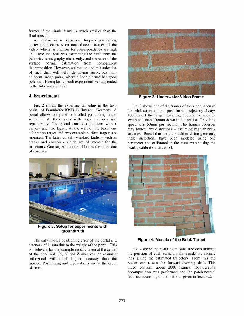
Figure 3: Underwater Video Frame
Fig. 3 shows one of the frames of the video taken of
the brick-target using a push-broom trajectory always
400mm off the target travelling 500mm for each x-
swath and then 100mm down in z-direction. Traveling
speed was 50mm per second. The human observer
may notice lens distortions – assuming regular brick
structure. Recall that for the machine vision geometry
these distortions have been modeled using one
parameter and calibrated in the same water using the
nearby calibration target [9].
Figure 4: Mosaic of the Brick Target
Fig. 4 shows the resulting mosaic. Red dots indicate
the position of each camera main inside the mosaic
thus giving the estimated trajectory. From this the
reader can assess the forward-chaining drift. This
video contains about 2000 frames. Homography
decomposition was performed and the patch-normal
rectified according to the methods given in Sect. 3.2.
777

778

Additional experiments were made with a different
camera displaying pincushion distortion (in contrast to
the barrel distortion visible in Figure 5). One frame is
displayed in Figure 7. Mosaicing runs quite the same
(after setting the internal camera parameters according
to the new calibration) and Figure 8 displays the result.
Here, the camera path was closed, so that a single
loop-closure following Meidow [7] could be applied
afterwards. The gain from such global method can be
seen in Figure 9.
5. Discussion
Of course we have also conducted experiments
with floating platforms and handheld cameras in
outdoor waters where the visibility conditions are
usually worse. This will also have an effect on the
errors. However, for the time being, we have no
groundtruth of the trajectory and orientations for such
videos. The portal made it possible to conduct the
experiments under water. Experiments in air would be
less representative for the underwater inspection task
because off the influence of the optical density of the
medium on the mapping geometry. E.g. the location of
the virtual projection center is not easy to be
determined, causing error in the calibration of the
focal length. It is also important to use the same
lighting conditions as will be used on inspection
cruises.
We conclude that under such benign visibility
conditions and with enough observable structure the
reported drift errors are small enough for automatic
underwater infrastructure inspection.
References
[1] A. Elibol, B. Moeller, R. Garcia, R. Perspectives of
Auto-Correcting Lens Distortions in Mosaic-Based
Underwater Navigation. Proc. of 23rd IEEE Int.
Symposium on Computer and Information Sciences
(ISCIS '08), Istanbul, Turkey, 1-6. October 2008.
[2] O. Faugeras, F. Lustman. Motion and structure from
motion in a piecewise planar environment. International
Journal of Pattern Recognition and Artificial
Intelligence, 2(3), 485–508, 1988.
[3] W. Foerstner. Minimal Representations for Uncertainty
and Estimation in Projective Spaces. ACCV (2), 619-632,
2010
[4] N. Gracias, J. Santos-Victor. Underwater Video Mosaics
as Visual Navigation Maps. Computer Vision and Image
Understanding, 79(1): 66-91, July 2000.
[5] M. Ludvigsen, B. Sortland, G. Johnsen, H. Sing.
Underwater Photo Mosaics in Marine Biology and
Archaeology. Oceanography, 20 (4), 140-149, 2007.
[6] P.F. McLauchlan, A. Jaenicke: Image Mosaicing Using
Bundle Adjustment. Image and Vision Computing, 20,
751-759, 2002.
[7] J. Meidow. Efficient Video Mosaicking by Multiple
Loop Closing. In: U. Stilla, (ed.). PIA 2011. Springer,
Berlin, (LNCS 6952), 2-12, 2011.
[8] E. Michaelsen, W. von Hansen, M. Kirchof, J. Meidow,
U. Stilla, U. Estimating the Essential Matrix:
GOODSAC versus RANSAC. In: W. Foerstner, R.
Steffen (eds) Proceedings Photogrammetric Computer
Vision and Image Analysis. International Archives of
Photogrammetry, Remote Sensing and Spatial
Information Science, Vol. XXXVI Part 3. 2006.
[9] E. Michaelsen. Stitching Large Maps from Videos Taken
by a Camera Moving close over a Plane Using
Homography Decomposition. ISPRS Conference( CD),
PIA 2011. München, CD Vol.: XXXVIII, Part 3/ W22, 5,
2011.
[10] E. Michaelsen. N. Scherer-Negenborn. Grouping and
Establishing Correspondence of Calibration Holes for
Underwater Machine Vision. Pattern Recongnition and
Image Understanding, accepted for appearance in 2012.
[11] N. Scherer-Negenborn, R. Schäfer. Model Fitting with
Sufficient Random Sample Coverage. International
Journal of Computer Vision, 89(1): 120-128, 2010.
[12] H. S. Sawhney, S. Hsu, and R. Kumar: Robust Video
Mosaicing through Topology Inference and Local to
Global Alignment. ECCV 98, Vol. 2, 103-119, 1998.
[13] Wikipedia: IRLS, last accessed April, 4th, 2012,
http://en.wikipedia.org/wiki/Iteratively_reweighted_least
_squares
779