ESTIMATING THE PRODUCTION FUNCTION FOR HUMAN CAPITAL: RESULTS FROM A RANDOMIZED CONTROL TRIAL IN COLOMBIA

By

Orazio Attanasio, Sarah Cattan, Emla Fitzsimons, Costas Meghir, and Marta Rubio-Codina

February 2015

COWLES FOUNDATION DISCUSSION PAPER NO. 1987

COWLES FOUNDATION FOR RESEARCH IN ECONOMICS YALE UNIVERSITY

Box 208281 New Haven, Connecticut 06520-8281

http://cowles.econ.yale.edu/

Estimating the Production Function for Human Capital:

Results from a Randomized Control Trial in Colombia

Orazio Attanasio, Sarah Cattan, Emla Fitzsimons,Costas Meghir, and Marta Rubio-Codina∗

February 11, 2015

Abstract

We examine the channels through which a randomized early childhoodintervention in Colombia led to significant gains in cognitive and socio-emotional skills among a sample of disadvantaged children. We estimateproduction functions for cognitive and socio-emotional skills as a func-tion of maternal skills and child’s past skills, as well as material andtime investments that are treated as endogenous. The effects of theprogram can be fully explained by increases in parental investments,which have strong effects on outcomes and are complementary to bothmaternal skills and child’s past skills.

∗Attanasio: University College London and Institute for Fiscal Studies (o.attanasio@ucl.ac.uk). Cat-tan: Institute for Fiscal Studies (sarah c@ifs.org.uk). Fitzsimons: UCL Institute of Education and Institutefor Fiscal Studies (e.fitzsimons@ioe.ac.uk). Meghir: Yale University, NBER, IZA and Institute for FiscalStudies (c.meghir@yale.edu). Rubio-Codina: Institute for Fiscal Studies and Inter-American DevelopmentBank (marta r@ifs.org.uk). We thank participants at the NBER Summer Institute, Barcelona GSE SummerForum and Montreal CIREQ Applied Microeconomics on Fertility and Child Development and seminars atStanford University, University of Chicago, Oxford University, Cornell University, Bristol University andthe Institute for Fiscal Studies for their comments. We are grateful to the Economic and Social ResearchCouncil (Grant ES/G015953/1), the Inter-American Development Bank, the International Growth Centre,and the World Bank for funding the intervention and data collection. Some of this research was financedby the European Research Council’s Advanced Grant 249612 and by the Grand Challenges Canada PrimeAward 0072-03 (sub-award reference number 560450). Sarah Cattan gratefully acknowledges financial assis-tance from the British Academy Postdoctoral Fellowship pf140104, as well as from the European ResearchCouncil’s Grant Agreement No. 240910. Costas Meghir thanks the Cowles foundation and the ISPS at Yalefor financial assistance. All errors are the responsibility of the authors.

1 Introduction

The first five years of life lay the basis for lifelong outcomes (Almond and

Currie, 2011). Due to rapid brain development and its malleability during

the early years (Knudsen, 2004; Knudsen et al., 2006), investments during

this period may play a crucial role in the process of human capital accumula-

tion. At this time, many children are, however, exposed to risk factors such

as poverty, malnutrition and non-stimulating home environments preventing

them from reaching their full potential and perpetuating poverty, particularly

in developing countries (McGregor et al., 2007).

There is increasing evidence that early childhood interventions can allevi-

ate the consequences of these detrimental factors in a long-lasting fashion. Ex-

amples include the Jamaica study (Gertler et al., 2014; Grantham-McGregor

et al., 1991; Walker et al., 2011) and the Perry Preschool program (Heck-

man et al., 2010). However, less is known about the behavioural mechanisms

through which these interventions affect children and their families.

This paper aims to examine the channels through which an early years in-

tervention in Colombia led to significant gains in cognitive and socio-emotional

skills among a sample of disadvantaged children. The intervention we study

was a randomized control trial that targeted children between 12 and 24

months old, for a period of 18 months, in families who are beneficiaries of

the conditional cash transfer program in Colombia (Familias en Accion). Its

structure mirrored that of the Jamaica intervention in that it included a psy-

chosocial stimulation component and a micro-nutrient supplementation com-

ponent. The psychosocial stimulation program, which we focus on in this

1

paper, provided weekly home visits to mothers of children, for a period of 18

months, with the aim of improving parenting practices in the early years and

beyond.

The short-term impact evaluation of the intervention reveals that psychoso-

cial stimulation had significant positive effects on the language and cognitive

development of children who received the home visits (Attanasio et al., 2014).

In what follows, we reproduce these results and also show impacts of the

intervention in other dimensions, such as indicators of socio-emotional devel-

opment. However, these results could have been generated by a number of

different mechanisms. In addition to the weekly, one-hour home visit during

which the child and their mother interacted with the home visitor, the inter-

vention could have altered parental investment behavior by making them aware

of the importance of early investments and informing them about parenting

practices that enhance the child’s learning at home.

In order to shed light on the mechanisms through which the stimulation

program affected child development, we estimate parents’ investment func-

tions and the production functions for cognitive and socio-emotional skills.

Following Cunha, Heckman, and Schennach (2010), we model the accumu-

lation of future skills as a process that is determined by the child’s current

stock of skills, parents’ investments and parental human capital as well as

(unobservable) shocks. This technology is non-linear and allows the degree of

substitutability between inputs to be determined from the data. We consider

two types of investment (time and commodities) and allow parental choices

to be endogenously determined by estimating investment functions that de-

2

pend on resources and prices. This approach provides a natural framework

to interpret and understand the potential channels through which the psy-

chosocial stimulation component of the intervention could have boosted the

skills of treated children. In particular, the intervention could have shifted

the distribution of parental investments and/or changed the parameters of

the production function, for example by making parents more productive or

effective.

To estimate the production functions for cognitive and socio-emotional

skills, we use data we collected both before and after the intervention in Colom-

bia. The data contain very rich measures of child development, maternal skills

and parental investments. Even with such rich data, estimating the parame-

ters governing the skill formation process remains challenging for two reasons.

First, inputs and outputs are likely to be measured with error. Second, inputs,

especially investments, can be endogenous if parental investment decisions re-

spond to shocks or inputs that are unobserved to the econometrician. To deal

with the measurement error issue, we use dynamic latent factor models as

Cunha, Heckman, and Schennach (2010). The endogeneity of investment is

taken into account by implementing a control function approach, as in Attana-

sio, Meghir, and Nix (2015), whose estimation procedure we adopt here. The

exclusion restrictions needed for identification are justified by the economics

of the model.

Our estimates of the production function reveal a series of interesting and

important findings. First, in line with the existing literature, we find strong

evidence that a child’s current stock of skills fosters the development of future

3

skills.1 Second, and also in line with the existing literature, we find that current

skills, parental investments and maternal human capital are complementary

in the production of future skills. Parental investments matter greatly for

the accumulation of skills. In particular, material investments seem to matter

more for cognitive skills, while time investments seem to matter more for socio-

emotional skills. Our results indicate that the parameters that determine the

productivity of investment greatly depend on whether investment is considered

endogenous. Ignoring the fact that parents choose investment leads to a large

downward bias of the estimated productivity of investment in the production

functions, therefore indicating that parents use investment to compensate for

negative shocks. Interestingly, this result is also obtained by Cunha, Heckman,

and Schennach (2010) and Attanasio, Meghir, and Nix (2015), yet in very

different contexts.2

With respect to the mechanisms through which the intervention oper-

ated, we find that the intervention significantly increased parental investments

among treated families compared to non-treated ones. At the same time, there

are no significant shifts in the parameters of the production function induced

by the intervention. These two findings mean that the gains in cognitive and

socio-emotional skills among children who received the intervention are fully

1These features of the technology of skill formation are often referred to as self-productivity and cross-productivity (Cunha et al., 2006).

2The former use the Children of the National Longitudinal Survey of Youth 1979, alongitudinal panel following the children of a representative sample of women born between1956 and 1964 in the US. The latter use the Young Lives Survey for India, a longitudinalsurvey following the lives of children in two age-groups: a Younger Cohort of 2,000 childrenwho were aged between 6 and 18 months when Round 1 of the survey was carried out in2002, and an Older Cohort of 1,000 children then aged between 7.5 and 8.5 years. Thesurvey was carried out again in late 2006 and in 2009 (when the younger children wereabout 8 the same age as the Older Cohort when the research started in 2002).

4

explained by the shift in investments.

Our findings make important contributions to the literature on human cap-

ital development, especially during the early years. To the best of our knowl-

edge, our paper is the first to estimate the technology of skill formation in the

first three years of life and to quantify the size of the dynamic complemen-

tarities between different domains of human development at such young ages.

Characterising the production function at various ages is key for the identifi-

cation of critical periods that are important to target for the development of

particular skills. Our paper and that of Attanasio, Meghir, and Nix (2015)

are the first to estimate non-linear production functions in a developing coun-

try context.3 Helmers and Patnam (2011) estimate production functions with

Indian data, but they rely on a linear technology, which implies that inputs

are perfect substitutes for each other. Our results show that this assumption

is strongly rejected by the data and that accounting for complementarities

between inputs is of high importance. In this regard, our results are strikingly

consistent with those of Cunha, Heckman, and Schennach (2010) and Attana-

sio, Meghir, and Nix (2015), neither of whom can reject that the technology

of skill formation is Cobb-Douglas. Finally, we are the first to account for

multiple types of investments in children. We establish that distinguishing

between material and time investments is important for our understanding of

skill formation in the early years. These findings have important implications

for the design of future interventions.

While there is a vast literature evaluating the impact of early childhood

3Attanasio, Meghir, and Nix (2015) estimate nonlinear production functions for cogni-tion and health in India for children from 5-15, using the Young Lives Survey.

5

interventions on child development, our paper innovates by complementing the

information obtained from a randomized controlled trial of a specific interven-

tion with a completely specified model of skill formation and parental invest-

ment in order to understand the mechanisms behind the observed impacts. In

this sense, our paper shares the motivation of Heckman, Pinto, and Savelyev

(2013), who are interested in the channels through which the Perry Pre-School

Program produced gains in adult outcomes. Our focus and methodology, how-

ever, are different: Heckman, Pinto, and Savelyev (2013) perform a mediation

analysis that decomposes linearly the treatment effects on adult outcomes into

components attributable to early changes in different personality traits. We

use a structural model in which parents make investment choices and human

capital accumulates according to a completely specified production function

to interpret and explain the impacts induced by a successful intervention. We

explicitly test alternative and specific hypothesis about the origin of the im-

pacts. Despite these differences, along with Heckman, Pinto, and Savelyev

(2013) and a few other papers (Attanasio, Meghir, and Santiago, 2012; Du-

flo, Hanna, and Ryan, 2012; Todd and Wolpin, 2006), our paper illustrates

how data from randomized trials can be profitably combined with behavioral

models to go beyond the estimation of experimentally induced treatment ef-

fects and interpret the mechanisms underlying them, a crucial step for policy

analysis.

The paper proceeds as follows. Section 2 describes the intervention and

the data collected pre- and post-intervention and summarizes the short-term

impacts of the intervention. Section 3 presents the theoretical framework we

6

use and discusses its identification. Section 4 describes our estimation strategy.

Section 5 presents the estimates of the model and discusses their implications

for our understanding of the intervention. Section 6 concludes.

2 The intervention, its evaluation and its impacts

Although some influential studies have shown that well-designed and well-

targeted interventions can achieve spectacular results that are sustained over

long periods of time, a key challenge remains in the design of interventions that

can be deployed on a large scale at reasonable cost whilst at the same time

maintaining the quality that underlies the observed impacts. In this study,

we use data from the evaluation of an intervention that was designed as an

effectiveness rather than an efficacy trial as it was deployed on a relatively

large scale and was delivered by local people. In this section, we give some

details on the intervention and its evaluation design.

2.1 The intervention design

The integrated early childhood program analyzed in this paper was targeted

at children aged between 12 and 24 months living in families receiving the

Colombian CCT program (Familias en Accion), which targets the poorest

20% of households in the country. The intervention lasted 18 months, starting

in early 2010. Appendix A contains a detailed description of the program’s

design, implementation and delivery. Here we summarize the key aspects.

The program was implemented in semi-urban municipalities in three re-

gions of central Colombia, covering an area three times the size of England.

7

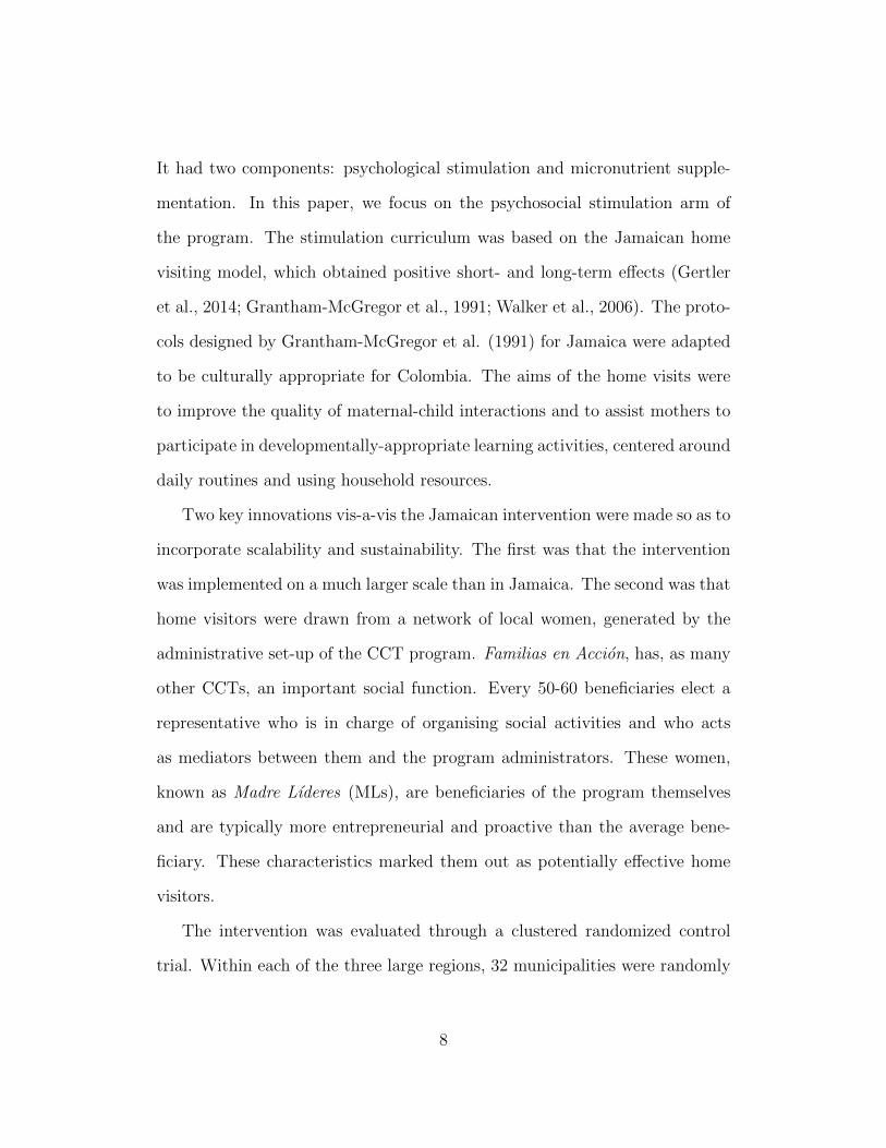
It had two components: psychological stimulation and micronutrient supple-

mentation. In this paper, we focus on the psychosocial stimulation arm of

the program. The stimulation curriculum was based on the Jamaican home

visiting model, which obtained positive short- and long-term effects (Gertler

et al., 2014; Grantham-McGregor et al., 1991; Walker et al., 2006). The proto-

cols designed by Grantham-McGregor et al. (1991) for Jamaica were adapted

to be culturally appropriate for Colombia. The aims of the home visits were

to improve the quality of maternal-child interactions and to assist mothers to

participate in developmentally-appropriate learning activities, centered around

daily routines and using household resources.

Two key innovations vis-a-vis the Jamaican intervention were made so as to

incorporate scalability and sustainability. The first was that the intervention

was implemented on a much larger scale than in Jamaica. The second was that

home visitors were drawn from a network of local women, generated by the

administrative set-up of the CCT program. Familias en Accion, has, as many

other CCTs, an important social function. Every 50-60 beneficiaries elect a

representative who is in charge of organising social activities and who acts

as mediators between them and the program administrators. These women,

known as Madre Lıderes (MLs), are beneficiaries of the program themselves

and are typically more entrepreneurial and proactive than the average bene-

ficiary. These characteristics marked them out as potentially effective home

visitors.

The intervention was evaluated through a clustered randomized control

trial. Within each of the three large regions, 32 municipalities were randomly

8

assigned to one of 4 groups: (i) psychosocial stimulation, (ii) micronutrient

supplementation, (iii) both, and (iv) control. Assignment to treatment was

via cluster-level randomization. In each municipality, 3 MLs were selected and

the children of the beneficiary households represented by each of these MLs

and aged 12-24 months, were recruited to the study. Therefore, there was a

total of 1,429 children living in 96 towns in central Colombia.

We conducted a baseline survey before the intervention started and a

follow-up survey when it ended 18 months later. The surveys took place in the

household, and children’s development was measured directly by psychologists

in community centers. The household surveys contain information on a rich set

of socio-economic and demographic characteristics as well as less standard vari-

ables such as children’s food intake, pre-school participation, maternal verbal

ability and mental health, and maternal knowledge and information, amongst

other things. We also collected information on stimulation in the home as

reported by the mother, using the UNICEF Family Care Indicators (FCI)

(Frongillo, Sywulka, and Kariger, 2003). This instrument includes questions

about the types and numbers of play materials around the house and about

the types and frequency of play activities the child engages in with an adult

aged 15 or more (most often the mother).

Children’s cognitive, language and motor development were assessed us-

ing the Bayley Scales of Infant and Toddler Development III, administered

directly in community centers (Bayley, 2006). Children’s language develop-

ment was also assessed through maternal report using a Spanish adaptation of

the short version of the MacArthur-Bates Communicative Development Inven-

9

tory (Jackson-Maldonado, Marchman, and Fernald, 2012). Children’s socio-

emotional development was also measured through maternal report using the

Bates’ Infant Characteristics Questionnaire (Bates, Freeland, and Lounsbury,

1979) and the Early Children’s Behavior Questionnaire (Putnam, Gartstein,

and Rothbart, 2006). All of these tests were administered both pre- and post-

intervention (using age-appropriate items), with the exception of the Early

Children’s Behavior Questionnaire which was only administered at follow-up.

We describe them at length in Appendix B.

2.2 The short-term impacts of the intervention

2.2.1 Impacts on child development

The top panel of Table 1 summarizes the short-term impact of the intervention

on measures of cognitive and socio-emotional development, some of which are

reported in Attanasio et al. (2014).4 The short-term impact evaluation of the

home visits showed an increase of 0.24 of a standard deviation (SD) in cognitive

development and an increase of 0.17 SD in receptive language, assessed using

the Bayley Scales of Infant and Toddler Development (Bayley-III).5

The lower panel of the table also shows that the intervention led to an im-

4At baseline, we administered the Bayley-III to 1,420 children and the survey to 1,429households (Figure 1). We excluded from analyses two children who scored less than threestandard deviations below the mean on the Bayley-III cognitive subscale. The attritionrate between baseline and follow-up for the Bayley-III sample was approximately 10.62%(n=153) across treatment arms: 36 (10.00%) of the children from the stimulation arm werenot measured at follow-up, 47 (13.06%) from the supplementation arm, 39 (10.83%) fromthe combined arm and 31 (8.61%) from the control arm. The difference in loss among thegroups was not statistically significant.

5These treatment effects are slightly different from those reported in Attanasio et al.(2014) because in this paper we estimate the impact of psychosocial stimulation by poolingthe two groups that received it and the two groups that did not, while Attanasio et al.(2014) estimates the impact of each of the four arms of the intervention separately.

10

provement in some dimensions of socio-emotional development. In particular,

it resulted in a 0.07 SD decrease in the dimension of the Bates scale measuring

difficult behavior; none of the other three components of the Bates scale were

significantly affected, however.

As discussed in greater length in Attanasio et al. (2014), no significant

impact of micro-nutrient supplementation on any child developmental out-

comes were found. As a result, in this paper, we focus on understanding

the effect of the psychosocial stimulation program on cognitive, language and

socio-emotional development.

2.2.2 Suggestive evidence of mechanisms

There are various mechanisms through which the psychosocial stimulation pro-

gram could have been effective in improving children’s cognitive, language and

socio-emotional development. The one-hour weekly visit aimed at providing

mothers with information on early childhood development and demonstrating

to them various developmental play activities they could repeat with their

child in between weekly home visits. The materials and toys used in the visit

were left in the home for the week following the visit in order to promote

increased interaction (both quality and quantity) between mother and child

on an ongoing basis. This should have subsequently affected positively var-

ious aspects of the child’s home environment, as well as the mother, whose

self-esteem, mental health6 and parenting activities might have improved.

6We tested for impacts of the intervention on the mother’s mental health, years ofeducation, IQ, vocabulary and maternal knowledge as measured by the Knowledge of InfantDevelopment Inventory (KIDI) (see Appendix B for a detailed description of the scales we useto measure these dimensions). We did not detect any significant impacts on these dimensions

11

The lower panel of Table 1 summarizes some of the results from the short-

term evaluation. These show large increases in intervention areas in the vari-

eties of play materials and play activities in the home, as measured by the FCI.

This is indicative that one mechanism through which home visits might have

improved child development was by promoting parental investments in chil-

dren. In order to test this hypothesis and assess the extent to which changes in

parental investments contributed to the observed impacts of the intervention,

we need a framework to understand the process of child development. We

use a production function to model the relationship between inputs and the

output of skill, which we describe below.

3 The accumulation of human capital in the early years:

a theoretical framework

In the previous section, we reported some of the impacts that an early years

intervention had both on children developmental outcomes and on parental

behavior. These estimates were straightforward to obtain due to the presence

of a cluster randomized control trial designed to evaluate the intervention. We

now build a theoretical framework that can be used to interpret and under-

stand these results.

In particular, we use a production function to describe the process through

which the skills of children evolve between the beginning and the end of the

intervention. We refer to the baseline period as t, when children were aged

of mothers’ human capital and therefore only report impacts on parental investments asmeasured by the FCI in Table 1. We return to this issue later in the paper.

12

Tab

le1:

Shor

t-te

rmim

pac

tsof

psy

cho-

soci

alst

imula

tion

onco

gnit

ion,

langu

age,

and

find

mot

ordev

elop

men

t;ch

ild

tem

per

amen

t;an

dpar

enta

lin

vest

men

ts

Inst

rum

ent:

Item

: C

ogn

itiv

eL

angu

age

rece

pti

ve

Lan

gu

age

exp

ress

ive

Fin

e m

oto

r V

oca

bu

lary

Co

mp

lex

sen

ten

ces

Tre

atm

ent

effe

ct

0.2

44

**

0.1

75

**

0.0

32

00

.07

13

0.0

94

70

.06

06

(0.0

62

1)

(0.0

64

7)

(0.0

62

3)

(0.0

61

7)

(0.0

65

2)

(0.0

56

3)

Ob

serv

atio

ns

1,2

64

1,2

64

1,2

62

1,2

61

1,3

21

1,3

21

Inst

rum

ent

Item

:U

nso

ciab

le

Dif

ficu

ltU

nad

apta

ble

Un

sto

pp

able

Var

ieti

es o

f p

lay

mat

eria

ls

Var

ieti

es o

f p

lay

acti

vit

ies

Tre

atm

ent

-0.0

43

3-0

.07

58

+0

.05

97

-0.0

31

30

.21

3*

*0

.27

3*

*

(0.0

54

9)

(0.0

45

5)

(0.0

61

5)

(0.0

53

5)

(0.0

63

7)

(0.0

49

9)

Ob

serv

atio

ns

1,3

26

1,3

26

1,3

26

1,3

26

1,3

26

1,3

26

Mac

Art

hu

r-B

ates

Bat

es

Fam

ily C

are

Ind

icat

ors

(F

CI)

Bay

ley

Not

es:

Th

eu

nit

ofob

serv

atio

nis

the

chil

d.

Coeffi

cien

tsan

dst

an

dard

erro

rs(i

np

are

nth

eses

)fr

om

are

gre

ssio

nof

the

dep

end

ent

vari

able

mea

sure

dat

foll

ow-u

pon

the

inte

rven

tion

vari

ab

le(a

trea

tmen

td

um

my

for

psy

choso

cial

stim

ula

tion

,co

mb

inin

gch

ild

ren

rece

ivin

gst

imu

lati

onal

one

and

chil

dre

nre

ceiv

ing

both

stim

ula

tion

an

dm

icro

-nu

trie

nt

sup

ple

men

tati

on

)co

ntr

oll

ing

for:

chil

d’s

sex;

bas

elin

ele

vel

ofth

eou

tcom

e(e

xce

pt

for

Mac

Art

hu

r-B

ate

s“C

om

ple

xse

nte

nce

s”,

wh

ere

we

contr

ol

for

base

lin

enu

mb

erof

word

ssp

oken

bec

ause

the

item

mea

suri

ng

“Com

ple

xse

nte

nce

s”w

as

not

mea

sure

dat

base

lin

e);

an

dte

ster

du

mm

ies.

Sta

nd

ard

erro

rsare

ad

just

edfo

rcl

ust

erin

gat

the

mu

nic

ipal

ity

leve

l.**

,*

an

d+

ind

icate

sign

ifica

nce

at

1,

5,

an

d10%

.A

llsc

ore

sh

ave

bee

nin

tern

all

yst

an

dard

ized

non

-par

amet

rica

lly

for

age

and

are

ther

efor

eex

pre

ssed

inst

an

dard

dev

iati

on

s(s

eeA

pp

end

ixB

for

det

ail

sab

ou

tth

em

easu

res

an

dth

est

and

ard

izat

ion

pro

ced

ure

).

13

between 12 to 24 months old, and to the post-intervention period as t + 1,

when children were aged between 30 to 42 months old. Children’s skills at

time t+ 1 are assumed to be a function of the vector of skills at t, of parental

skills, of parental investments and of some shocks. Our first aim is to charac-

terize such a function and estimate its parameters. We assume that parents

choose investments in human capital, reflecting their taste, their resources and

information about the current evolution of skills. Together with the produc-

tion function we estimate an investment function. Finally, we explicitly allow

for measurement error of all the relevant variables that enter the production

function and are determined by it: child and parents’ skills as well as parents’

investment.

Within this framework, the intervention can affect the accumulation of

skills through different channels. For example, the intervention can change

the parameters of the production function or can change parents’ investment

behavior. To allow for these effects, we let some of the parameters of the

production function and of the investment function depend on the (randomly

allocated) intervention.

Because we only focus on the effect of the psychosocial stimulation pro-

gram, we define the non-treated group (d = 0) as the group of children who

did not receive the home visits (therefore including both the control group

and the group who only received the micro-nutrients) and the treated group

(d = 1) as the group of children who received the home visits (therefore in-

cluding those who received only the home visits and those who received both

the home visits and the micro-nutrients).

14

3.1 The production function for human capital

We consider a two-dimensional vector of skills, which includes cognitive and

socio-emotional skills. In the baseline period, child i’s skills are denoted

θi,t = (θCi,t, θSi,t), where θCi,t and θSi,t are cognitive and socio-emotional skills

at t, respectively. At the end of the intervention, the child’s skills are denoted

θi,t+1 = (θCi,t+1, θSi,t+1).

Following Cunha, Heckman, and Schennach (2010), we assume that the

stock of skills in period t + 1 is determined by the baseline stock of the

child’s cognitive and socio-emotional skills θi,t, the mother’s cognitive and

socio-emotional skills, denoted by PCi,t and P S

i,t respectively, and the invest-

ments Ii,t made by the parents between t and t + 1.7 We also allow for the

effect of a variable ηki,t that reflects unobserved shock or omitted inputs. As

with skills, parental investments Ii,t can be a multi-dimensional vector. Here,

we distinguish between material and time investments, which we denote as IMi,t

and ITi,t respectively.

For each skill, we assume the production function is of the Constant Elas-

ticity of Substitution (CES) type, so we can write the technology of formation

for skill k as follows:

θki,t+1 =Akd[γk1,dθ

Ci,t

ρk + γk2,dθSi,t

ρk + γk3,dPCi,t

ρk + γk4,dPSi,t

ρk

+ γk5,dIMi,t

ρk + γk6,dITi,t

ρk ]1ρk eη

ki,t k ∈ {C, S}

(1)

where Akd is a factor-neutral productivity parameter and ρk ∈ (−∞, 1] deter-

7Note that because the mother is the main caregiver in most families, we focus on herskills as those that are most likely to influence the child’s development.

15

mines the elasticity of substitution, given by 1/(1−ρk), between the inputs af-

fecting the accumulation of skill k. Under such parameterization, as ρk → −∞,

the inputs become perfect complements. As ρk → 1, the inputs become perfect

substitutes. Notice that we let all the parameters of the production function,

except the elasticity of substitution ρk, be a function of the intervention. This

choice is dictated by our interpretation of how the intervention could have

generated the impacts documented above.

First, the intervention could have changed the parameters of the production

function that determine productivity. For example, by providing information

about good parenting practices, the intervention could have increased the qual-

ity of the investments. In the framework above, this could be reflected by a

shift in the factor-neutral productivity parameter Akd between the treated and

the non-treated group or a shift in particular share parameters γkj,d. Second,

the intervention could have affected IMi,t and ITi,t, the level of material and time

investments that parents make, as suggested by the results presented in Ta-

ble 1. For this reason we will let the parameters of the investment function,

which we describe below, be a function of the intervention. In addition, the

intervention could also have affected mothers’ skills, for instance by improving

self-esteem and reducing depression, or maternal knowledge as measured by

the Knowledge of Infant Development Inventory (KIDI). Although we checked

for these impacts, we did not detect any differences in measures of maternal

human capital between control and treated after the intervention, so going for-

ward we assume this mechanism away. From now on, we will therefore assume

that mother’s human capital is time-invariant and denote her cognitive and

16

socio-emotional skills by PCi and P S

i .

A few other features of the production function should be noted. First, all

the parameters are specific to a particular skill, so the productivity parameter,

the share parameters and the elasticity substitution can differ between the

production function of the cognitive skills and that of the socio-emotional

skills. Second, the CES functional form provides a great level of flexibility

in that it allows the degree of substitutability between the various inputs

of the production function to be determined by the data and to range from

perfect substitutes to perfect complements. One well-known limitation of the

CES functional form is that it imposes the same elasticity of substitution

between any two inputs. This could, of course, be alleviated by estimating

more general production functions, and in preliminary work we experimented

with nested CES production functions. We could not reject the CES functional

form however and so we maintain this functional form assumption throughout

the application.

There are two main challenges to identifying and estimating the production

functions outlined above. The first is related to the fact that parents choose

investment in children, so that investments are likely to be correlated with

the unobserved shock ηki,t. The second issue is that children’s skills, as well as

parental investments and maternal skills, could be measured with error in the

data. We discuss how we tackle these two issues in the sub-sections below.

17

3.2 Accounting for the endogeneity of parental investments

The first issue that complicates the identification of the production function

outlined above is the possibility that parental investments are endogenous,

which would arise if E(ηki,t|Ii,t) 6= 0. There are two main reasons why parental

investments might be correlated with the unobserved shock affecting the ac-

cumulation of human capital. First, parental investments might be correlated

with omitted inputs in the production function of the child’s skills. Second,

parental investments might respond to unobserved, time-varying shocks in or-

der to compensate or reinforce their effects on child development. Consider,

for example, the case of a child who is suddenly affected by a negative shock,

such as an illness, which is unobserved to the econometrician but perceived

by the parents as delaying the child’s development. As a result of this shock,

parents might decide to invest in their child’s development more than they

would have otherwise. This parental response would create a negative correla-

tion between parental investments and the unobserved shock ηki,t affecting the

development of skills of type k, which would lead the estimate of the effect

of parental investments on future skill to be downward biased. Alternative

assumptions about preferences and technologies (or technologies as perceived

by the parents) can create different patterns of correlations between shocks

and investment and, therefore, introduce different types of biases.

Endogeneity, of course, arises because parents choose investment in chil-

dren to maximize some objective function taking into account the technology

of human capital accumulation, the costs of investment and the resources avail-

able. In such a context, investment choices in any period will depend on initial

18

conditions, on the shocks affecting the child and observed by the parent, on

prices and on total resources. Rather than modeling investment choices jointly

with the production function and making specific assumptions on taste (which

would imply a specific functional form for the investment function), we esti-

mate a reduced form equation that should be interpreted as an approximation

of the investment function. We then use this approximation to implement

a control function approach in the estimation of the production function for

human capital and, therefore, control for the endogeneity of investment.

For identification, our approach requires that some variables that deter-

mine investment choices do not enter the production function directly. A

natural candidate would be the intervention we described above, as it was

allocated randomly across villages. However, as we want to test whether the

intervention changed the parameters of the production function, we cannot

use it as an exclusion restriction and need additional variables for valid identi-

fication. Moreover, as we model separately different forms of investment, the

intervention alone would not be sufficient.

Following Cunha, Heckman, and Schennach (2010), we assume that, for

each factor k, the error term ηki,t can be decomposed into two components, πki,t

and υki,t. The production function can then be re-written in logs as:

ln(θki,t+1) =1

ρkln[γk1,dθ

Ci,t

ρk + γk2,dθSi,t

ρk + γk3,dPCi

ρk + γk4,dPSi

ρk + γk5,dIMi,t

ρk

+γk6,dITi,t

ρk ] + ln(Akd) + δkπki,t + υki,t, k = {C, S}(2)

Both πkt and υk,t are assumed to be distributed independently across children.

However, πkt is assumed to be realized before parents make investment choices

19

and therefore can influence their choices, whereas υki,t is realized after parents

make investment choices. The goal of the control function approach is to

recover a consistent estimate of πki,t, so that it can be controlled for when

estimating the production function. This in turn requires estimating a model

of investment.

As discussed above, we do not derive explicit investment functions from a

complete structural model. Instead, we specify an approximation to non-linear

investment functions as log-linear equations in initial conditions, maternal

skills and the variables Zi,t, representing resources and prices:

ln(Iτi,t) =λτd,0 + λτd,1 ln(θCi,t) + λτd,2 ln(θNi,t) + λτd,3 ln(PCi ) + λτd,4 ln(P S

i )

+ λτd,5 ln(Zi,t) + uτi,t, τ = {M,T}(3)

where uτi,t is a linear combination of πCi,t and πSi,t. Note that all parameters of

the investment functions, including the intercept, are allowed to vary between

the treated and non-treated groups. This reflects the possibility, discussed

above, that the intervention changed parental investment strategies.

Once the parameters of the investment functions are estimated, we recover

uTi,t and uMi,t , the estimated residuals from the investment equations (3), which

we include as regressors when estimating the production functions:

ln(θki,t+1) =1

ρkln[γk1,dθ

Ci,t

ρk + γk2,dθSi,t

ρk + γk3,dPCi,t

ρk + γk4,dPSi,t

ρk + γk5,dIMi,t

ρk

+ γk6,dITi,t

ρk ] + ln(Akd) + φkM uMi,t + φkT u

Ti,t + υki,t, k = C,N

(4)

Identification of the parameters of the production function rests on the as-

20

sumption that the disturbances πki,t and υki,t in equation (2) are independent of

Zi,t and that there are at least as many exclusion restrictions – variables that

affect the technology of skill formation only through the investment process

– as there are endogenous variables. Economic theory suggests that variables

that exogenously shift the household’s resources might be valid exclusion re-

strictions, since they impact parental investment decisions through the budget

constraint without entering directly the production function. In this spirit, we

use average male and female wages in the child’s village, household’s wealth at

baseline, and an indicator for whether the mother is married as variables that

determine resources but do not enter the production function explicitly. These

variables are valid exclusion restrictions insofar as, conditional on the child’s

skills at baseline and maternal human capital, they are orthogonal to πkt . We

believe that this assumption is likely to hold, as we control for a multitude of

child and parents’ characteristics through the latent factors.

One of the variables we use as a determinant of investment that does not

enter the production function is household wealth. One could argue that

household wealth is endogenous to unobserved shocks affecting the child. In-

deed, going back to our example above, it is possible that parents of a sick

child decide to work more and increase their wealth in order to bolster the

care they can provide him or her. Our strategy is less likely to suffer from

this caveat, however, because we use baseline measures of wealth that should

precede any shocks occurring between t and t+ 1. Moreover, excluding wealth

from the investment functions does not change the point estimates but only

affects precision.

21

3.3 Measurement of skills and investments

As described in section 2.2, the data contains multiple measures of the inputs

and outputs of the production functions specified above. These measures are

likely to proxy a lower-dimensional vector of skills and investment, but to do so

with some error. In order to deal with this issue, we follow Cunha, Heckman,

and Schennach (2010) in using latent factor models and we estimate the joint

distribution of error-ridden latent factors measuring children’s skills at baseline

(θCt and θSt ), children’s skills at follow-up (θCt+1 and θSt+1), mother’s skills (PC

and P S) and parental investments (IMt and ITt ), where we keep the individual

subscript i implicit for notational simplicity. Our specific estimation approach

follows the procedure developed in Attanasio, Meghir, and Nix (2015) and is

detailed in the next section.

Suppose we have M1k,t measures of child’s skills of type k (k ∈ {C, S}) at

time t. We also have M2k measures of maternal skills of type k (k ∈ {C, S})

and M3τ,t measures of parental investments of type τ (τ = {M,T}) at t.8

Let m1k,t,j denote the jth measure of child’s skill of type k at t, m2

k,j the jth

measure of mother’s skill of type k, and m3τ,t,j the jth measure of parental

investment of type τ at t. As is common in the psychometric literature, we

assume a dedicated measurement system, that is one in which each measure

only proxies one factor (Gorusch, 1983, 2003).9 Assuming each measure is

8The measures of maternal skills are not indexed by time because we have assumed theyare time-invariant.

9This assumption is not necessary for identification, but we choose to specify a dedicatedmeasurement system so as to make the interpretation of the latent factors more transparent.As described in Appendix C, we find clear support in the data for such a system.

22

additively separable in the (log) of the latent factor it proxies,10 we can write:

m1k,t,j = µ1

k,t,j + α1k,t,j ln θkt + ε1k,t,j (5)

m2k,j = µ2

k,j + α2k,j lnP k + ε2k,j (6)

m3τ,t,j = µ3

τ,t,j + α3τ,t,j ln Iτt + ε3τ,t,j (7)

where the terms µ1k,t,j, µ

2k,j and µ3

τ,t,j are intercepts, the terms α1k,t,j, α

2k,j and

α3τ,t,j are factor loadings, and the terms ε1k,t,j, ε

2k,j and ε3τ,t,j are measurement

errors. Note that the latent factors can be freely correlated with each other.

An important specificity of our application of latent factors models is that

we consider an intervention and aim to capture its effect on the entire dis-

tribution of latent factors. To do so, we allow the joint distribution of the

latent factors to be completely different between the two treatment states

(d = {0, 1}). In contrast, we assume that the intercepts, factor loadings and

measurement errors are invariant across states. These assumptions imply that

any difference in the distribution of measures between the control and treated

groups result from differences in the distribution of the latent factors and not

from differences in the measurement system for those factors. As discussed in

Heckman, Pinto, and Savelyev (2013), these assumptions are sufficient but not

necessary for identification. We maintain them in our application because they

restrict the number of free parameters and lead to improvements in efficiency.

Additionally, because the treatment was randomized successfully, there is no

reason to think that these parameters should vary across groups.

10We specify the measurement equation such that measures proxy the log of a latentfactor so that latent factors only take positive values.

23

Because the latent factors are unobserved, identification of factor models

requires normalizations to set their scale and location (Anderson and Rubin,

1956). We set the scale of the factors by setting the factor loading of the

first measure of each latent factor to 1, that is: α1k,t,1 = α2

k,1 = α3τ,t,1 = 1,

∀t, τ = {M,T} and k = {C, S}. We set the location of the factors by fixing

the mean of the latent factors to 0 in one group. Without loss of generality,

we do so in the control group (d = 0) and allow the latent factor means of the

treated group to be freely estimated.11

Under these normalizations, Heckman, Pinto, and Savelyev (2013) show

that identification of the system is guaranteed as long as we have at least three

measures dedicated to each factor under the assumptions that the measure-

ment error is independent across measures and from the latent factors and that

E(ε1k,t,j) = E(ε2k,j) = E(ε3τ,t,j) = 0 for j ∈ {1, . . . ,M1k,t; 1, . . . ,M2

k; 1, . . . ,M3τ,t},

∀t, k ∈ {C, S} and τ ∈ {M,T}.

Note that some of these assumptions could be relaxed (Carneiro, Hansen,

and Heckman, 2003; Cunha and Heckman, 2008; Cunha, Heckman, and Schen-

nach, 2010). For instance, the same measure could be allowed to load on sev-

eral factors, as long as there are some dedicated measures. It would also be

possible to allow measurement error to be correlated across measures of the

same factor, as long as there was one measure whose measurement error was

independent from the measurement error in other measures of the same factor.

11This normalization is innocuous because, without it, we would identify the differencein factor means between the treatment and control groups, which is exactly the object ofinterest.

24

4 Estimation of the model

The approach we use to estimate our model is described in detail in Attanasio,

Meghir, and Nix (2015) and involves two main stages. In the first, we estimate

the joint distribution of the latent factors; in the second, we estimate the

parameters of the investment and production functions, using draws from the

joint distribution of factors.

4.1 First stage: estimating the joint distribution of latent factors

As mentioned above, using the Kotlarski theorem and its extensions by Carneiro,

Hansen, and Heckman (2003), Cunha and Heckman (2008) and Cunha, Heck-

man, and Schennach (2010), the model is non-parametrically identified. For

estimation however, we make some distributional assumptions for the distri-

bution of latent factors and measurement error. In particular, we assume that

the latent factors are distributed as a mixture of two joint log-normal distri-

butions. The mixture of log normal distribution represents a flexible way to

approximate a generic distribution. In principle, one could allow for a mixture

of three or more log normal distributions for even greater flexibility, but in

our application, we found the two-type mixture satisfactory. Note that it is

important to allow for substantial deviation from normality, as such a func-

tional form would imply linearity (or log-linearity in the case of log normality)

of the conditional means and, in turn, restrict the elasticity of substitution

among factors (for example, normality of the factors would imply that inputs

are perfectly substitutable.)

For notational brevity, we denote from now on the vector of latent factors as

25

θ = (θCt+1, θSt+1, θ

Ct , θ

St , P

C , P S, IMt , ITt ). As mentioned above, we allow the joint

distribution of θ to be fully-specific to each intervention group d (d ∈ {0, 1})

so their density function in group s can be written as:

pd(ln θ) = τdpd(ln θA) + (1− τd)pd(ln θB) (8)

where ln θA ∼ N(µAd ,ΣAd ) and ln θB ∼ N(µAd ,Σ

Ad ) and τd is the mixture weight.

In addition, we assume that the measurement errors are distributed as a joint

normal distribution with means 0 and diagonal variance-covariance Σε. Notice

that an implication of the additive separability of the measurement equations

(5) - (7), together with the assumption of log-normality of the factors and of

normality of the additive measurement error, is that the joint distribution of

measurements is given by a mixture of normals.

We first estimate the parameters of the joint distribution of measurements

by maximum likelihood, using the EM algorithm. We then map these param-

eters into the parameters of the joint distribution of factors, the variances of

measurement errors, the factor loadings and the intercepts and obtain esti-

mates of these parameters by minimum distance. We report the relationships

between the parameters of the distribution of measurements and those of the

distribution of factors and of measurement errors in Appendix C. A more detail

treatment of the approach is found in Attanasio, Meghir, and Nix (2015).

4.2 Second stage: estimating investment and production functions

Once the joint distribution of latent factors is estimated for each group d,

we can estimate the investment functions and the production functions using

26

draws from the estimated distributions as data. Given draws on all the la-

tent factors, we first estimate the log-linear investment functions by ordinary

least squares and construct the residuals uτt (τ ∈ {M,T}) that serve as con-

trol functions. As mentioned above, we let the parameters of the investment

function depend on the intervention, reflecting the fact that the intervention

might have changed the way parents behave. Next, we estimate the param-

eters of the CES production functions by non-linear least squares, including

the estimated residuals of the investment functions as additional regressors, as

specified in equation (4).

To highlight the bias resulting from failing to account for the endogeneity

of investments, we present results with and without control functions. We

compute standard errors and confidence intervals using the bootstrap.12

4.3 Specification of the empirical model

In addition to the factors capturing the child’s skills at baseline and mother’s

skills, in the production function, we include the number of children in the

household (as measured at follow-up). This is to allow for the possibility that

the presence of siblings affects child development, either because of spillover

effects or by reducing the level of attention parents devote to each one of

their children in multiple children households. We also include the number

of children as a determinant of investment, which we suspect might depend

negatively on the number of siblings. Since the number of children in the

12We draw Q = 1000 bootstrap samples of the original data, accounting for the fact thatthe data is clustered at the village level, and we apply the estimation procedure describedabove to each one of the pseudo-sample. For each of the parameters, we then compute thestandard deviation of its distribution based on its Q = 1000 bootstrapped values, alongwith various percentiles to compute the corresponding confidence intervals.

27

household enters the production function directly, it does not enter our list of

exclusion restrictions.

To compute our measure of household wealth, we add to the measurement

system described above a set of measures from the baseline survey that proxy

an additional latent factor measuring household wealth with error. These mea-

sures are described in full in Table 2 below and include indicators of whether

the household owns its dwelling, along with various other assets (fridge, car,

computer, etc.). The other exclusion restrictions (average male and female

wages in the village and whether the mother is married), as well as the vari-

able measuring the number of children in the household, are assumed not to

have any measurement error.13

5 Results

We start by reporting the estimates of the measurement system, followed by

the estimates of the investment and production functions. Finally, armed with

these parameters, we assess how the model fits the data and how it helps us

interpret the impact of the early years intervention we have studied.

13To estimate the joint distribution of all the data we need to estimate the investmentand production functions, we therefore specify a measurement system that comprises ofall the measures of child’s skills, mother’s skills, investments and household wealth, alongwith these four additional variables. Each of these four variables can be thought of beinga function of a latent factor and a measurement error term (following the same structureas equation (5) for example), but in their case, the variance of measurement error is 0 andthe associated factor loading is 1. With respect to male and female wages in the village, wetook an average of male and females wages reported by members of the sample and in doingso rid the average of the measurement error possibly contained in individual observations.

28

Tab

le2:

Mea

sure

men

tsy

stem

and

sign

al-t

o-noi

sera

tio

for

each

mea

sure

s

Fac

tor

Mea

sure

s C

on

tro

lsT

rea

ted

F

acto

r M

easu

res

Co

ntr

ols

Tre

ate

d

Bay

ley C

ogn

itiv

e 7

6%

77

%N

um

ber

of

dif

fere

nt

pla

y m

ater

ials

9

6%

97

%

Bay

ley R

ecep

tive

Lan

gu

age

71

%7

2%

Nu

mb

er o

f co

lou

rin

g b

oo

ks

44

%4

6%

Bay

ley E

xp

ress

ive

Lan

gu

age

78

%7

9%

Nu

mb

er o

f to

ys

bo

ugh

t6

5%

67

%

Bay

ley F

ine

Mo

tor

55

%5

7%

Nu

mb

er o

f to

ys

that

req

uir

e m

ovem

ent

73

%7

5%

Mac

Art

hu

r-B

ates

Vo

cab

ula

ry

55

%5

6%

Nu

mb

er o

f to

ys

to l

earn

sh

apes

7

3%

75

%

Mac

Art

hu

r-B

ates

Co

mp

lex

Sen

ten

ces

38

%3

9%

Nu

mb

er o

f d

iffe

ren

t p

lay a

ctiv

itie

s 9

5%

98

%

Bay

ley C

ogn

itiv

e*7

4%

67

%T

imes

to

ld a

sto

ry t

o c

hil

d i

n l

ast

3 d

ays

67

%8

3%

Bay

ley R

ecep

tive

Lan

gu

age*

80

%7

4%

Tim

es r

ead

to

ch

ild

in

las

t 3

day

s 7

0%

85

%

Bay

ley E

xp

ress

ive

Lan

gu

age*

80

%7

3%

Tim

es p

layed

wit

h c

hil

d a

nd

to

ys

in l

ast

3 d

ays

64

%8

1%

Bay

ley F

ine

Mo

tor*

68

%6

0%

Tim

es l

abel

led

th

ings

to c

hil

d i

n l

ast

3 d

ays

65

%8

2%

Mac

Art

hu

r-B

ates

Vo

cab

ula

ry*

43

%3

5%

Mo

ther

s' y

ears

of

edu

cati

on

*6

4%

63

%

Bat

es D

iffi

cult

su

b-s

cale

(-)

69

%6

7%

Mo

ther

's v

oca

bu

lary

7

0%

69

%

Bat

es U

nso

ciab

le s

ub

-sca

le (

-)2

1%

20

%N

um

ber

of

bo

oks

for

adu

lts

in t

he

ho

use

*

40

%3

9%

Bat

es U

nst

op

pab

le s

ub

-sca

le (

-)6

2%

60

%N

um

ber

of

mag

azin

es a

nd

new

spap

ers

18

%1

7%

Ro

thb

art

Inh

ibit

ory

Co

ntr

ol

sub

-sca

le7

0%

68

%R

aven

's s

core

("I

Q")

**

60

%5

9%

Ro

thb

art

Att

enti

on

su

b-s

cale

25

%2

4%

Did

yo

u f

eel

dep

ress

ed?

(-)

42

%4

6%

Bat

es D

iffi

cult

fac

tor*

(-)

67

%7

2%

Bo

ther

ed b

y w

hat

usu

ally

do

n't

bo

ther

yo

u?

(-)

28

%3

2%

Bat

es U

nso

ciab

le f

acto

r* (

-)1

9%

23

%H

ad t

rou

ble

kee

pin

g m

ind

on

do

ing?

(-)

35

%3

8%

Bat

es U

nad

apta

ble

* (

-)3

4%

40

%F

elt

ever

yth

ing y

ou

did

was

an

eff

ort

? (-

)3

1%

34

%

Bat

es U

nst

op

pab

le*

(-)

23

%2

8%

Did

yo

u f

eel

fear

ful?

(-)

24

%2

7%

Ow

ns

a fr

idge

39

%4

0%

Did

yo

u s

leep

was

res

tles

s? (

-)3

0%

34

%

Ow

ns

a ca

r 6

%6

%D

id y

ou

fee

l h

app

y?

(-)

13

%1

5%

Ow

ns

a co

mp

ute

r 3

4%

35

%H

ow

oft

en d

id y

ou

fee

l lo

nel

y l

ast

wee

k?

(-)

31

%3

5%

Ow

ns

a b

len

der

28

%2

9%

Did

yo

u f

eel

yo

u c

ou

ldn

't get

go

ing?

(-)

39

%4

2%

Ow

n a

was

hin

g m

ach

ing

8%

8%

Ow

ns

dw

elli

ng

11

%1

1%

Ow

ns

a ra

dio

1

2%

13

%

Ow

s a

TV

3

2%

33

%

Wea

lth

% S

ign

al

% S

ign

al

Ch

ild

's

cogn

itiv

e

skil

ls

(t+

1)

Ch

ild

's

cogn

itiv

e

skil

ls

(t)

Ch

ild

's s

oci

o-

emo

tio

nal

skil

ls (

t+1

)

Ch

ild

's s

oci

o-

emo

tio

nal

skil

ls (

t)

Mo

ther

's

soci

o-

emo

tio

nal

skil

ls

Tim

e

inves

tmen

ts

Mo

ther

's

cogn

itiv

e

skil

ls

Mat

eria

l

inves

tmen

ts

Note

:T

his

tab

lesh

ows

the

mea

sure

sal

low

edto

load

on

each

late

nt

fact

or,

as

wel

las

the

fract

ion

of

the

vari

an

cein

each

mea

sure

that

isex

pla

ined

by

the

vari

ance

insi

gnal

,fo

rth

eco

ntr

olan

dtr

eatm

ent

gro

up

sse

para

tely

.M

easu

res

foll

owed

by

an

ast

eris

ks

(*)

wer

eco

llec

ted

at

base

lin

ean

dm

easu

res

foll

owed

by

two

aste

risk

s(*

*)w

ere

coll

ecte

dat

follow

-up

II.

All

oth

erm

easu

res

wer

eco

llec

ted

at

foll

ow-u

pI

at

the

end

of

the

inte

rven

tion

.T

he

sign

(-)

foll

owin

gm

easu

res

ofth

ech

ild

’sn

on-c

ogn

itiv

esk

ill

an

dth

em

oth

er’s

non

-cogn

itiv

esk

ill

ind

icate

sth

at

the

scori

ng

on

thes

em

easu

res

was

reve

rsed

soth

atth

eco

rres

pon

din

gla

tent

fact

or

issu

chth

at

ah

igher

score

mea

ns

ah

igh

erle

vel

of

non

-cogn

itiv

esk

ill.

5.1 The measurement system and the distribution of factors

Table 2 describes the specification of the measurement system, which underlies

the estimates of the production function, that is the set of variables used as

measures of each latent factor. To arrive at this specification, we performed an

exploratory factor analysis of the data that helped us to determine the number

of factors that could be extracted from the data and to allocate measures to

particular factors. The steps and results of this exploratory factor analysis are

discussed in detail in Appendix C.

As mentioned above, identification requires that at least one measure for

each factor is conditionally independent of the other measures for the same

factor. In our case, this assumption can be justified by the fact that some

developmental outcome variables are based on child level observations and

are collected by a trained psychologist in community centers, while others are

based on maternal reports and are collected in the home (on a different day)

by an interviewer. The independence of measurement errors is probably not a

far fetched assumption in such a context.

From the first stage of the estimation procedure, we obtained estimates of

the measurement system, i.e. estimates of the mean and variance-covariance

matrix of the latent factors for each group d = {0, 1}, estimates of the factor

loadings and of the variances of the measurement error.14 All these parameter

estimates are reported in Appendix C.15 Using these estimates, it is possible to

14We standardized all measures with respect to their mean in the control group, so webypass the estimation of the intercepts.

15More precisely, Appendix Table A3 reports the estimates of the factor loadings in eachmeasurement equation. Appendix Table A4 reports the estimates of the means of the latentfactor distributions for the treated households relative to the means of the latent factor

30

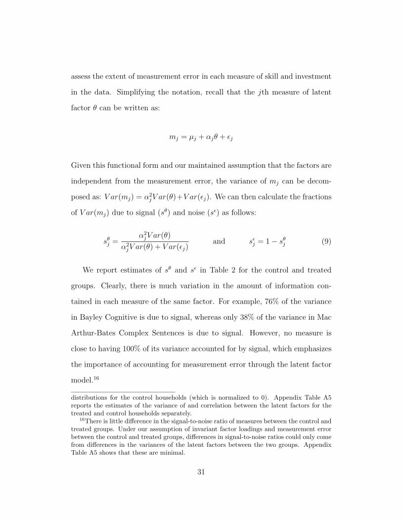
assess the extent of measurement error in each measure of skill and investment

in the data. Simplifying the notation, recall that the jth measure of latent

factor θ can be written as:

mj = µj + αjθ + εj

Given this functional form and our maintained assumption that the factors are

independent from the measurement error, the variance of mj can be decom-

posed as: V ar(mj) = α2jV ar(θ)+V ar(εj). We can then calculate the fractions

of V ar(mj) due to signal (sθ) and noise (sε) as follows:

sθj =α2jV ar(θ)

α2jV ar(θ) + V ar(εj)

and sεj = 1− sθj (9)

We report estimates of sθ and sε in Table 2 for the control and treated

groups. Clearly, there is much variation in the amount of information con-

tained in each measure of the same factor. For example, 76% of the variance

in Bayley Cognitive is due to signal, whereas only 38% of the variance in Mac

Arthur-Bates Complex Sentences is due to signal. However, no measure is

close to having 100% of its variance accounted for by signal, which emphasizes

the importance of accounting for measurement error through the latent factor

model.16

distributions for the control households (which is normalized to 0). Appendix Table A5reports the estimates of the variance of and correlation between the latent factors for thetreated and control households separately.

16There is little difference in the signal-to-noise ratio of measures between the control andtreated groups. Under our assumption of invariant factor loadings and measurement errorbetween the control and treated groups, differences in signal-to-noise ratios could only comefrom differences in the variances of the latent factors between the two groups. AppendixTable A5 shows that these are minimal.

31

Figure 1: Kernel densities of latent factors

(a) Children’s cognitive skills, baseline

−3 −2 −1 0 1 2 3

0.0

0.1

0.2

0.3

0.4

0.5

Den

sity

TreatedControl

(b) Children’s socio-emotional skills, baseline

−3 −2 −1 0 1 2 3

0.0

0.1

0.2

0.3

0.4

0.5

Den

sity

TreatedControl

(c) Children’s cognitive skills, follow-up

−3 −2 −1 0 1 2 3

0.0

0.1

0.2

0.3

0.4

0.5

Den

sity

TreatedControl

(d) Children’s socio-emotional skills, follow-up

−3 −2 −1 0 1 2 3

0.0

0.1

0.2

0.3

0.4

0.5

Den

sity

TreatedControl

(e) Material investments

−3 −2 −1 0 1 2 3

0.0

0.1

0.2

0.3

0.4

Den

sity

TreatedControl

(f) Time investments

−3 −2 −1 0 1 2 3

0.0

0.1

0.2

0.3

0.4

Den

sity

TreatedControl

Note: These kernel densities are constructed using 10,000 draws from the estimated jointdistribution of latent factors for the control group and for the treated group.

Having identified the entire distribution of factors for each group, we can

study whether the intervention has changed the entire shape of these distribu-

tions, in addition to their means. In Figure 1, we plot the estimated Kernel

densities of some of the factors. The first two panels show the distribution,

in treatment and control villages, of cognitive and socio-emotional skills at

baseline. These first two pictures confirm that our sample is substantially

balanced. The following two panels depict the distribution of cognitive and

socio-emotional factors at follow-up. In the case of cognitive factors we see

that the shift in the mean reported in Appendix Table A4 reflects a shift in

the entire distribution. For socio-emotional factors, however, the shift occurs

mainly for children below the median.

Finally, in the last two panels, we notice a strong shift to the right of both

the material and time investment factors. This suggests that at least part of

the impact of the intervention is likely to have been driven by increases in both

time and materials devoted by parents to the upbringing of their children.

5.2 Estimates of the investment functions

In Table 3, we present estimates of the investment equations. The first col-

umn presents the equation for material investments and the second column

for time investments. As far as we know, our paper is unique in distinguishing

between material and time investments in the context of estimating non-linear

technologies of skill formation. Note that the results reported in Table 3 ex-

clude interactions of the treatment parameter with the remaining variables.

In earlier versions we found such interactions to be insignificant, i.e. the shift

33

Table 3: Estimates of the log-linear investment function

Log of material

investments

Log of time

investments

Constant 0.001 0.004

(0.016) (0.015)

[-0.025,0.027] [-0.02,0.028]

Treatment dummy 0.248 0.361

(0.073) (0.065)

[0.115,0.349] [0.235,0.451]

Log of child's cognitive skills at t 0.141 0.116

(0.061) (0.057)

[0.032,0.231] [0.007,0.198]

Log of child's socio-emotional skills at t -0.008 0.031

(0.058) (0.056)

[-0.105,0.084] [-0.053,0.13]

Log of mother's cognitive skills 0.668 0.462

(0.082) (0.079)

[0.54,0.815] [0.317,0.573]

Log of mother's socio-emotional skills -0.120 -0.310

(0.074) (0.103)

[-0.25,-0.001] [-0.474,-0.123]

Log of wealth at t 0.081 -0.086

(0.071) (0.090)

[-0.019,0.217] [-0.231,0.06]

Mother is married at t+1 0.126 0.115

(0.027) (0.027)

[0.075,0.164] [0.066,0.155]

Log of number of children at t+1 -0.096 -0.090

(0.033) (0.033)

[-0.146,-0.04] [-0.151,-0.041]

Log of average male wages in village at t+1 0.075 -0.026

(0.041) (0.044)

[-0.007,0.117] [-0.106,0.039]

Log of average female wages in village at t+1 0.004 0.033

(0.038) (0.031)[-0.077,0.054] [-0.013,0.088]

Note: Standard errors in parentheses and 90% confidence intervals in brackets are obtainedusing the non-parametric bootstrap described in Section 4. Appendix B provides a detaileddescription of the variables used to measure each latent factor.

in investment seems to have been uniform across groups with differing back-

grounds.17

The first striking result is the impact of treatment on investments: it in-

creases resources by 25% and time by 36% and both effects are highly signifi-

cant. Thus, the intervention increased the time and the resources that parents

provide to children. Referring back to the measurement system (Table 2), it

is worthwhile noting that the time inputs are measured in a way that are tar-

geted to child educational activities, such as the number of times an adult read

to the child in the last three days. In other words, they do not refer simply to

time spent with the child, but to interactions that promote development. Sim-

ilarly, material investments refer to particular types of toys and play materials.

Importantly, our estimates of the impact of the intervention on investments

are uniquely driven by the experimental design and do not require any of the

assumptions necessary for the identification of the production functions.

Turning now to the other regressors, we find that both time and material

investments increase with the child’s cognitive skills, but socio-emotional skills

have no impact on investments, at least at the very young ages we are con-

sidering. The elasticity of both material and time investments with respect

to maternal cognition is very high and particularly so for the former; however

mother’s socio-emotional skills have no significant effect. Married mothers in-

17Appendix Table A6 reports the estimates of the investment equation in which weinteract all the regressors with the treatment dummy. We test the joint significance of theinteraction terms and find that we cannot reject that all the interactions are equal to 0 forboth material and time investments at conventional levels of significance (the p-value forthe material investment equation is 0.577 and the p-value for the time investment equationis 0.667). Appendix Table A7 reports the estimates of the production functions when thecontrol functions are derived from the fully interacted investment function. We observe nomajor difference between these results and the ones based on the non-interacted investmentfunction reported in Tables 4 and 5.

35

vest more time and more materials, but the overall number of children reduces

investments. We find no effect of wealth on investments, probably because

our sample is quite homogeneously poor. However, we do find that more is

invested in children in terms of materials when male wages are higher in the

village, which we interpret as an income effect. Average female wages in the

village, which could reflect the opportunity cost of time for the mother as well

as her access to resources, have no effect.

Of the above variables, wealth, marital status, and male and female wages

at the village level are excluded from the production function and serve as

instruments. We test for the joint significance of the exclusion restrictions

in the material and time investment equations. The p-value from a F-test

performed separately on each equation is 0.008 for the material investment

equation and 0.041 for the time investment equation. The p-value of a test

that the rank of the coefficient matrix of the excluded variables across both

investment equations is less than 2 has a p-value of 0.035.18 The fact that some

of the coefficients on the individual variables are not statistically different from

zero is probably driven by collinearity and by the limited variation we have

(as some of these variables only vary across village). From the high joint

significance of our instruments however, we conclude that they are strong

enough to identify the impact of investment in the production function for

skills, to which we now turn.

18To perform this rank test, we proceeded as follows. Let B be the 2 × 4 matrix ofcoefficients on the four excluded variables in the two investment equations. We used thenon-parametric bootstrap to derive critical values for a test that the smallest eigenvalueof B′B is zero. See Robin and Smith (2000) for a discussion of such tests and Blundell,Duncan, and Meghir (1998) for a similar application.

36

5.3 Estimates of the production functions

Tables 4 and 5 report the estimates of the CES production function. For each

skill, we report estimates of the parameters of the production function obtained

both ignoring the endogeneity of investments (in the left column) and taking

it into account by including the residuals from the investment functions as

additional inputs (in the right column), as specified in equation (4). It should

be stressed that very limited systematic evidence exists on the evolution and

development of children skills at such young ages.

We have experimented with allowing all coefficients to vary with treatment

status, but we found no evidence that the production function differs system-

atically as a result of the intervention. In fact the tests that the coefficients

are the same across intervention and control groups, other than total factor

productivity A, have p-values of 0.879 and 0.889 for the production functions

of cognitive and socio-emotional skills, respectively.19 Indeed, as Tables 4 and

5 show, even total factor productivity remains unaffected by treatment, ex-

cept when we treat investments as exogenous in the production function for

cognitive skills (first column of Table 4).20

The results provide evidence of several important features of skill devel-

opment. First, we find strong evidence of self-productivity of skills. That

is, the current stock of cognitive (socio-emotional) skills strongly affects the

19Appendix Tables A8 and A9 report the estimates of the production function for eachskill type in which we allow all parameters (except the elasticity of substitution) to varybetween treated and controls. None of the interactions, except that with the number ofchildren in the household, is significant.

20We also experimented with a specification of the model where we allowed the child’sage at follow-up to enter the investment equations and to interact with the total-factorproductivity parameter (A) in the production functions. We did not find evidence that thisparameter depended on the child’s age however (see Appendix Tables A10 and A11.)

37

Table 4: Estimates of the CES production function for cognitive skills

Without control

function

With control

function

Child's cognitive skills at t 0.591 0.566

(0.043) (0.057)

[0.527,0.67] [0.489,0.674]

Child's socio-emotional skills at t 0.03 0.038

(0.043) (0.050)

[-0.037,0.106] [-0.035,0.126]

Mother's cognitive skills 0.194 0.037

(0.049) (0.131)

[0.107,0.264] [-0.194,0.223]

Mother's socio-emotional skills 0.06 0.051

(0.045) (0.049)

[-0.016,0.126] [-0.028,0.127]

Material investments at t+1 0.082 0.397

(0.033) (0.208)

[0.036,0.144] [0.128,0.765]

Time investments at t+1 0.008 -0.138

(0.035) (0.142)

[-0.056,0.057] [-0.421,0.039]

Number of children in household at t+1 0.035 0.049

(0.026) (0.030)

[-0.009,0.076] [0.002,0.1]

Control function for material investments - -0.33

(0.218)

[-0.715,-0.023]

Control function for time investments - 0.156

(0.151)

[-0.037,0.453]

Complementarity parameter 0.123 0.07

(0.082) (0.060)

[-0.025,0.243] [-0.032,0.161]

Elasticity of substitution 1.141 1.075

(0.106) (0.070)

[0.976,1.321] [0.969,1.192]

Productivity parameter (A) 0.984 0.993

(0.012) (0.011)

[0.966,1.005] [0.972,1.008]

Productivity parameter interacted with treatment 0.1 0.08

(0.052) (0.072)

[0.028,0.198] [-0.012,0.228]

Note: Standard errors in parentheses and 90% confidence intervals in brackets are obtainedusing the non-parametric bootstrap described in Section 4. Appendix B provides a detaileddescription of the variables used to measure each latent factor.

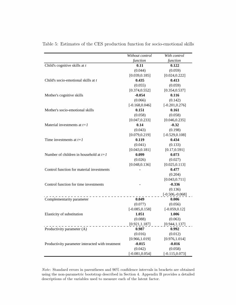
Table 5: Estimates of the CES production function for socio-emotional skills

Without control

function

With control

function

Child's cognitive skills at t 0.11 0.122

(0.044) (0.059)

[0.039,0.185] [0.024,0.222]

Child's socio-emotional skills at t 0.435 0.413

(0.055) (0.059)

[0.374,0.552] [0.354,0.537]

Mother's cognitive skills -0.054 0.116

(0.066) (0.142)

[-0.168,0.046] [-0.201,0.276]

Mother's socio-emotional skills 0.151 0.161

(0.058) (0.058)

[0.047,0.233] [0.046,0.235]

Material investments at t+1 0.14 -0.32

(0.043) (0.198)

[0.079,0.219] [-0.529,0.108]

Time investments at t+1 0.119 0.434

(0.041) (0.133)

[0.043,0.181] [0.17,0.591]

Number of children in household at t+1 0.099 0.073

(0.026) (0.027)

[0.048,0.136] [0.025,0.113]

Control function for material investments - 0.477

(0.204)

[0.043,0.711]

Control function for time investments - -0.336

(0.136)

[-0.506,-0.068]

Complementarity parameter 0.049 0.006

(0.077) (0.056)

[-0.085,0.158] [-0.059,0.12]

Elasticity of substitution 1.051 1.006

(0.088) (0.063)

[0.921,1.187] [0.944,1.137]

Productivity parameter (A) 0.987 0.992

(0.016) (0.012)

[0.966,1.019] [0.976,1.014]

Productivity parameter interacted with treatment -0.015 -0.016

(0.042) (0.058)

[-0.081,0.054] [-0.115,0.073]

Note: Standard errors in parentheses and 90% confidence intervals in brackets are obtainedusing the non-parametric bootstrap described in Section 4. Appendix B provides a detaileddescriptions of the variables used to measure each of the latent factor.

development of future (socio-emotional) cognitive skills. Second, we find ev-

idence of cross-productivity in the production function for socio-emotional

skills (Table 5): the current stock of cognitive skills fosters the development

of future socio-emotional skills. Although the current stock of socio-emotional

skills has a positive coefficient in the production function of cognitive skills,

the estimate is not significantly different from zero and we cannot conclude

there is cross-productivity in the production of cognitive skills. This result

contrasts with that reported by Cunha, Heckman, and Schennach (2010), who

find socio-emotional skills to be important for the accumulation of future cog-

nitive skills. Our evidence, however, relates to a different, much earlier, period

of the life-cycle.

Our results also provide evidence that parental investments play a crucial

role in the development of both cognitive and socio-emotional skills and that

they are endogenous. With respect to cognitive skills, the results reveal that

only material investments seem to matter; their effect becomes very large and

strongly significant, once we control for endogenous investments. With respect

to socio-emotional skills, when we treat investments as endogenous, only time

investments significantly matter for the accumulation of socio-emotional skills.

The point estimate of the share parameter for material investments is negative,

but very imprecise. The effect of time investments on future socio-emotional

skills is very large and strongly significant.

Investments are also clearly endogenous. The control function in the cog-

nitive production function is highly significant for material investments and

including it increases the share parameter for material investments more than

40

fivefold. Similarly the control function for time investments in the correspond-

ing production function is also highly significant, and including it in the pro-

duction function triples the coefficient on time investments. In both of these

cases, the estimate of the coefficient of the relevant control function is nega-

tive, suggesting that parents compensate with materials and time when adverse

events affect the development of their child. This evidence is important as it

speaks to the issue of whether parental investment reinforces or compensates

shocks received by children, an issue discussed by a large literature, some of

which is surveyed in Almond and Mazumder (2013). Our findings indicate very

clearly that investment seems to be compensating rather than reinforcing.

The estimates of the production functions show that mothers’ cognitive

skills do not seem to have a significant direct effect on either children’s cog-

nitive or socio-emotional development, once we control for the endogeneity of

investments. However, it should be remembered that according to our esti-

mates of the investment function (Table 3), mother’s cognitive skills have an

important effect on both types of investment and, therefore, an indirect ef-

fect on child development. Mother’s socio-emotional skills have a significant

impact on the development of the child’s socio-emotional skills, even after

controlling for the endogeneity of investments, but their effect on the child’s

future cognitive skills is not significantly different from zero.

It is also interesting that the number of siblings improves outcomes for

children conditional on investments, presumably because of mutual stimulation

and interaction. On the other hand, the estimates of the investment function

imply that siblings also dilute investments to the subject child, thus creating

41

two counteracting effects.

The last key component of the production function is the complementarity

parameter, ρk. In both production functions, it is estimated to be zero, which

implies an elasticity of substitution equal to one. That is, the production

function for cognitive and socio-emotional skills has a Cobb-Douglas form.

5.4 Implications for human capital accumulation and the role of

the intervention

The results presented above have interesting implications for human capital

accumulation. First, the production function is Cobb-Douglas and hence in-

puts are complementary. Moreover, baseline skills, investments and, to some

extent, maternal skills are important for the development of future skills. To-

gether, these two facts imply that investments are more productive for children

with higher levels of early cognition and socio-emotional skills.

We illustrate this point in Figure 2, which plots the marginal product of

investments as a function of the child’s baseline skills. Consider first Figure

2a. The productivity of material investment in the production function for

cognitive skills triples as we move from the lower deciles to the upper deciles

of the distribution of baseline cognition. Similarly, time investments are more

productive for the accumulation of socio-emotional skills, the higher a child

is on the distribution of socio-emotional skills at baseline (Figure 2b). This

complementarity illustrates both the importance of targeting low-achieving

children early as well as the difficulty of delivering interventions with high

returns for them, particularly as time passes.

42

43

Figure 2: Complementarity between investments and baseline skills

(a) Marginal product of material investments in the production of cognitive skills

Decile

Mar

gina

l pro

duct

of m

ater

ial i

nves

tmen

t

1 2 3 4 5 6 7 8 9 10

0.2

0.4

0.6

0.8

1.0

1.2

i.By decile of cognitive skills

Decile

1 2 3 4 5 6 7 8 9 100.

20.

40.

60.

81.

01.

2

ii.By decile of socio−emotional skills

(b) Marginal product of time investments in the production of socio-emotional skills

Decile

Mar

gina

l pro

duct

of t

ime

inve

stm

ent

1 2 3 4 5 6 7 8 9 10

0.2

0.4

0.6

0.8

1.0

i.By decile of cognitive skills

Decile

1 2 3 4 5 6 7 8 9 10

0.2

0.4

0.6

0.8

1.0

ii.By decile of socio−emotional skills

Notes: The marginal product of material and time investments in the production function

for skill of type k are given by: Akdγk5,dI

Mi,t

(ρk−1)Q(1−ρkρk

)and Akdγ

k6,dI

Ti,t

(ρk−1)Q(1−ρkρk

), re-

spectively, where Q = [γk1,d(θCi,t)

ρk + γk2,d(θSi,t)

ρk + γk3,d(PCi )ρk + γk4,d(P

Si )ρk + γk5,d(I

Mi,t )

ρk +

γK6,d(ITi,t)

ρk ]. The figures above are constructed by evaluating these objects at different

deciles of θCi,t (figures i) and θSi,t (figures ii) and holding all remaining inputs of the pro-duction function at their mean values pooling observations from the control and treatmentgroups together.

As we mentioned above, the factor-neutral productivity parameter A is not

shifted by the treatment indicator, whose coefficient is small and insignificant

in either production function. Moreover, when we test whether the interven-

tion has shifted any of the other parameters of the production function, we

cannot reject the null of no change. On the other hand, there is a positive and

significant shift in parental investments among treated families relative to non-

treated families (Figure 1), and on average there is a 25% increase in material

investments and 36% increase in time investments among treated households

relative to control households. These results imply that the intervention acted

exclusively by changing parental investments in materials and time and not

by increasing the productivity of investments nor that of any other inputs.

Given the evidence we just presented on the role that these investments play

in the production function for human capital, it is natural to ask whether this

channel can explain all the impact of the intervention.

More formally, we ask what fraction of the difference in skills between the

treated and non-treated children can be explained by the change in parental

investments induced by the intervention. We can answer this question by us-

ing the structure and estimates of the model. In particular, we predict the

distributions of future cognitive and socio-emotional skills given the distribu-

tion of investments in the treatment group and those of the control group

respectively. We then compute the gap between the two for each type of skill.

This difference measures how much of the impact of the intervention we can

explain using just the change in investments.

Table 6 reports the results from this exercise based on the estimates with

44

Table 6: Decomposition of the treatment effects in skills

Cognitive skills

at t+1

Socio-emotional skills

at t+1

Data 0.115 0.075

(0.056) (0.045)

[0.011,0.195] [0.007,0.151]

Model 0.107 0.088

(0.058) (0.047)

[0.009,0.195] [0.005,0.156]

Gap in log skills between treated and controls

Note: Standard errors in parentheses and 90% confidence intervals in brackets are obtainedusing the non-parametric bootstrap described in Section 4. Appendix B provides a detaileddescription of the variables used to measure each latent factor.

endogenous investments. The results indicate that the model predicts the

actual gap in log skills between the treated and non-treated children well

for both type of skills. Specifically the model predicts 93% of the cognitive

improvement and slightly overshoots the socio-emotional improvement among

treated children. The differences between the data and the model predictions

are not significant. Thus the conclusion is quite clear: the intervention changed

parental behavior by inducing more of the appropriate investments but did not

change the production function.

An interpretation of this finding is that, as a result of the intervention, par-

ents’ behavior did not become more productive in itself, but parents allocated

more of their resources on their children, given their beliefs on the effectiveness

of these investments. This suggests that a reason for under-investment in child

development among poor populations might be a lack of knowledge about the

45

effectiveness of investments, thus implying that one way interventions can be

successful is by changing parenting beliefs on the subject.

6 Conclusion

In this paper, we estimate the production functions for cognitive and socio-

emotional skills in early childhood and analyze the mechanisms through which

a randomized early childhood intervention in Colombia affected child develop-

ment. The intervention itself - a psychosocial stimulation program delivered

through weekly home visits - significantly improved the cognitive and socio-

emotional development of children aged between 12 and 24 months at the

start of the intervention. Underlying our approach is a model of parental in-

vestments in children, constrained by a production function for cognitive and

socio-emotional skills.

We make three interrelated contributions. First, we estimate equations

for material and time investments depending on both family and child base-

line characteristics. Second, we estimate production functions for cognitive

and socio-emotional skills that depend on the investments, which are taken

to be endogenous. Third, we use this framework to trace out the way the

intervention affected the production of children’s skills.

In line with the existing literature, we find strong evidence that a child’s

current stock of skills fosters the development of future skills (self-productivity).

We also find evidence that early cognition helps improve socio-emotional skills

(cross-productivity). Second, and also in line with the existing literature, we

find that current skills, parental investments and maternal human capital are

46

complementary in the production of future skills. This means, for example,

that parental investments are more productive when the child’s current skills

are higher. Lastly, we find that parental investments greatly matter for the

accumulation of cognitive and socio-emotional skills. In particular, material

investments seem to matter more for cognitive skills, while time investments

seem to matter more for socio-emotional skills. Our paper is the first to esti-

mate a non-linear production function for skills with different types of invest-

ments, and our results show that it is a non-trivial extension of the standard

model.

When we compare the production function estimates between treatment

and control groups, we cannot reject that they are the same. We find that

we can attribute the entire effect of the intervention to an increase in time

and material resources devoted by parents to their children. In other words,

the intervention did not shift the way that skills are produced. Nevertheless,

we show that even a shift in investments without a change in the produc-

tion function succeeded in altering children’s outcomes in significant ways.

Whether the intervention changed parental behavior fundamentally enough to

yield long-lasting impacts is an open question, but one of crucial importance

as further follow-up data is collected. The framework developed here surely

offers a valuable tool to understand what drives the sustainability of this and

other early years interventions and organize the evidence in a systematic way.

47

References

Almond, D. and Currie, J. (2011). Human capital development before age five.In O. Ashenfelter and D. Card, eds., Handbook of Labor Economics, Volume4b. Elsevier Science, Amsterdam.

Almond, D. and Mazumder, B. (2013). Fetal origins and parental responses.The Annual Review of Economics 5(3):1–20.

Anderson, T. and Rubin, H. (1956). Statistical inference in factor analysis.In Proceedings of the Third Berkeley Symposium on Mathematical Statisticsand Probability, volume 5, 111–150. University of California Press, Berkeley.

Attanasio, O., Fernandez, C., Fitzsimons, E., Grantham-McGregor, S.,Meghir, C., and Rubio-Codina, M. (2014). Using the infrastucture of aConditional Cash Transfer programme to deliver a scalable integrated earlychild development programme in Colombia: A cluster randomised controlledtrial. Forthcoming in British Medical Journal 349:g5785.

Attanasio, O., Meghir, C., and Nix, E. (2015). Investments in children andthe development of cognition and health in India. Mimeo, Yale University.

Attanasio, O., Meghir, C., and Santiago, A. (2012). Education choices inMexico: Using a structural model and a randomized experiment to evaluateProgresa. Review of Economic Studies 79(1):37–66.

Bates, J., Freeland, C., and Lounsbury, M. (1979). Measurement of infantdifficultness. Child Development 50:794–803.

Bayley, N. (2006). Bayley Scales of Infant and Toddler Development. HarcourtAssessment, San Antonio, TX, 3rd edition.

Blundell, R., Duncan, A., and Meghir, C. (1998). Estimating labor supplyresponses using tax reforms. Econometrica 66(4):827–761.

Carneiro, P., Hansen, K., and Heckman, J. (2003). Estimating distribution ofcounterfactuals with an application to the returns to schooling and measure-ment of the effect of uncertainty on schooling choice. International EconomicReview 44(2):361–422.

Cunha, F. and Heckman, J. (2008). Formulating, identifying and estimatingthe technology of cognitive and noncognitive skill formation. Journal ofHuman Resources 43(4):738–782.

48

Cunha, F., Heckman, J., Lochner, L., and Masterov, D. (2006). Interpretingthe evidence on life cycle skill formation. In E. Hanushek, S. Machin, andL. Woessmann, eds., Handbook of the Economics of Education, Volume 1.Elsevier Science, Amsterdam.

Cunha, F., Heckman, J., and Schennach, S. (2010). Estimating the technologyof cognitive and non-cognitive skill formation. Econometrica 78(3):883–931.

Duflo, E., Hanna, R., and Ryan, S. P. (2012). Incentives work: Getting teach-ers to come to school. American Economic Review 102(4):1241–78.

Frongillo, E., Sywulka, S., and Kariger, P. (2003). UNICEF psychosocial careindicators project. Final report to UNICEF. Mimeo, Cornell University.

Gertler, P., Heckman, J., Pinto, R., Zanolini, A., Vermeerch, C., Walker, S.,Chang, S., and Grantham-McGregor, S. (2014). Labor market returns to anearly childhood stimulation intervention in Jamaica. Forthcoming, Science.

Gorusch, R. (1983). Factor Analysis. Lawrence Erlbaum Associates, Hillsdale,NJ.

Gorusch, R. (2003). Factor analysis. In Handbook of psychology: Researchmethods in psychology, volume 2, 143–164. John Wiely & Sons, Inc., Hobo-ken, NJ.

Grantham-McGregor, S., Powell, C., Walker, S., and Himes, J. (1991). Nutri-tional supplementation, psychosocial stimulation, and mental developmentof stunted children: the Jamaican study. Lancet 338(758):1–5.

Heckman, J., Moon, S., Pinto, R., Savelyev, P., and Yavitz, A. (2010). Ana-lyzing social experiments as implemented: A reexamination of the evidencefrom the HighScope Perry Preschool Program. Journal of Quantitative Eco-nomics 1:1–46.

Heckman, J., Pinto, R., and Savelyev, P. (2013). Understanding the mecha-nisms through which an influential early childhood program boosted adultoutcomes. American Economic Review 103:2052–2086.

Helmers, C. and Patnam, M. (2011). The formation and evolution of childhoodskill acquisition: Evidence from India. Journal of Development Economics95(2):252–266.

49

Jackson-Maldonado, D., Marchman, V., and Fernald, L. (2012). Short formversions of the Spanish MacArthur-Bates Communicative Development In-ventories. In Applied Psycholinguistics. Cambridge University Press, Cam-bridge.

Knudsen, E. (2004). Sensitive periods in the development of the brain andbehavior. Journal of Cognitive Neuroscience 16(1):1412–1425.

Knudsen, E., Heckman, J., Cameron, J., and Shonkoff, J. (2006). Economic,neurobiological and behavioral perspectives on building America’s futureworkforce. Proceedings of the National Academy of Science 103(27):10155–10162.

McGregor, S. G., Cheung, Y., Cueto, S., Glewwe, P., Richter, L., and Strupp,B. (2007). Developmental potential in the first 5 years for children in devel-oping countries. The Lancet 369(9555):60–70.

Putnam, S. P., Gartstein, M., and Rothbart, M. K. (2006). Measurement offine-grained aspects of toddler temperament: The Early Childhood BehaviorQuestionnaire. Infant Behavior and Development 29(3):386–401.

Robin, J. and Smith, R. (2000). Tests of rank. Econometric Theory 16:151–175.

Todd, P. and Wolpin, K. (2006). Using experimental data to validate a dy-namic behavioral model of child schooling and fertility: Assessing the im-pact of a school subsidy program in Mexico. American Economic Review96(5):1384–1417.

Walker, S., Chang, S., C.Powell, E.Simonoff, and Grantham-McGregor, S.(2006). Effects of psychosocial stimulation and dietary supplementation inearly childhood on psychosocial functioning in late adolescence: follow-upof randomized controlled trial. British Medical Journal 333(7566):472.

Walker, S., Chang, S., Vera-Hernandez, M., and Grantham-McGregor, S.(2011). Early childhood stimulation benefits adult competence and reducesviolent behavior. Pediatrics 127(5):849–857.

50

Estimating the Production Function for Human Capital:

Results from a Randomized Control Trial in Colombia

Orazio Attanasio, Sarah Cattan, Emla Fitzsimons,Costas Meghir, and Marta Rubio-Codina∗

APPENDIX FOR ONLINE PUBLICATION

February 7, 2015

∗Attanasio: University College London and Institute for Fiscal Studies (o.attanasio@ucl.ac.uk). Cattan:Institute for Fiscal Studies (sarah c@ifs.org.uk). Fitzsimons: UCL Institute of Education and Institute forFiscal Studies (e.fitzsimons@ioe.ac.uk). Meghir: Yale University, NBER and Institute for Fiscal Studies(c.meghir@yale.edu). Rubio-Codina: Institute for Fiscal Studies and Inter-American Development Bank(marta r@ifs.org.uk). We thank participants at the NBER Summer Institute, Barcelona GSE Summer Fo-rum and Montreal CIREQ Applied Microeconomics on Fertility and Child Development and seminars atStanford University, University of Chicago, Oxford University, Cornell University, Bristol University andthe Institute for Fiscal Studies for their comments. We are grateful to the Economic and Social ResearchCouncil (Grant ES/G015953/1), the Inter-American Development Bank, the International Growth Centre,and the World Bank for funding the intervention and data collection. Some of this research was financedby the European Research Council’s Advanced Grant 249612 and by the Grand Challenges Canada PrimeAward 0072-03 (sub-award reference number 560450). Sarah Cattan gratefully acknowledges financial assis-tance from the British Academy Postdoctoral Fellowship pf140104, as well as from the European ResearchCouncil’s Grant Agreement No. 240910. Costas Meghir thanks the Cowles foundation and the ISPS at Yalefor financial assistance. All errors are the responsibility of the authors.

A The Intervention

This appendix provides a detailed description of the intervention, its imple-

mentation and roll-out. The material in this section draws heavily on Attana-

sio et al. (2014).

A.1 Description of the Intervention

The integrated early child development intervention was designed so that it

could be delivered by local people, readily identifiable through administrative

infrastructures of social welfare systems (the conditional cash transfer program

Familias en Accion (FeA) in our case). The intervention included psychosocial

stimulation on its own, micronutrient supplementation on its own, and both

combined. Each of these arms had 24 clusters (municipalities).

A.1.1 Psychosocial Stimulation

The psychosocial stimulation component was inspired by and based on the

Jamaican home visiting model (Walker et al 2011), the overarching aim of

which is to facilitate developmentally appropriate learning activities between

mothers (primary caregivers) and their children through demonstration of play

activities centred around daily routines. Play activities draw on resources in

the home, low cost home-made toys and the intervention toy kit. The toy kit

included picture books, naming plates, conversation scenes, puzzles, lotteries,

and blocks. Play activities followed steps aimed towards children’s gradual

mastery of a learning objective: (1) child observes play activity (modeling),

2

(2) mother and child do the activity together, (3) child attempts the play

activity on his/her own, (4) mother prompts naming and verbalisation of ob-

jects and actions linked to the play activity, (5) the developmental level of

play activity is adjusted by increasing or decreasing the challenge based on

the child’s performance (scaffolding). Throughout the play activities, mothers

are encouraged to provide children with contingent positive reinforcement for

progress toward the learning goals (praise) and to follow the child’s interest.

Materials for the stimulation component were adapted from the Jamaican

intervention guide to the local cultural context and to the average educational

level of home visitors and program beneficiaries. Such adaptations included

(1) inclusion of local songs and rhymes; (2) modification of the home-made

toys instruction manual to use local recyclable materials, (3) incorporation

into the the intervention toy kit of culturally relevant pictures, scenes and

objects, (4) re-organization of the psychosocial stimulation guide in weekly

instruction cards for specific age groups, and (5) ordering of play materials,

via an index, by developmental stage to facilitate the scaffolding of activities.

Home visits lasted approximately one hour. Home visits took place with

the child’s biological mother or primary caregiver. Other adults in the house-

hold, where present, were also encouraged to participate in the home visit. In

advance of the visit, the home visitor selected the weekly instruction card from

the psychosocial stimulation guide according to the appropriate developmental

level of the target child, and prepared the toys and materials for the visit. The

home visit had three parts. At the beginning, the home visitor did an informal

assessment of the child’s progress in the sequence of play activities, by asking

3

about the play activities the mother and child practiced during the previous

week and identifying where challenges arose (or on the contrary, where activi-

ties were overly simplistic). In the second and main part of the visit, new play

activities were shown and practised. At the end, the mother was prompted to

summarize the play activities and agree a plan on how to practice them over

the following week.

A.1.2 Micronutrient Supplementation

The micronutrient supplementation component consisted of micronutrient sup-

plementation in the form of sprinkles (encapsulated micronutrients). Each

single-dose sachet contains 12.5 mg iron, 5 mg zinc, vitamin A 300 mg RE,

160mg g folic acid and 30 mg vitamin C and each displayed a pictorial represen-

tation of use. In addition to the fortnightly provision of sprinkles, participating

families received a booklet with detailed instructions for use and storage and

daily record forms to track use. Families were provided with enough sachets

for all children below six years of age to prevent sharing with siblings.

A.2 Implementation

We obtained institutional cooperation from the National Director of FeA, the

coordinator of the Strategic Planning and Monitoring Unit of FeA, and FeA

administrative staff at the municipality level. From the latter, we obtained

rosters of female community representatives (Madres Lideres) and selected

three female community representatives in each of the 96 target municipalities.

In municipalities assigned to receive stimulation, 63% of selected female

4

community leaders took on the role of home visitor. The remainder declined

due to other work commitments or not meeting the minimum reading compre-

hension criteria (established using a short reading comprehension test designed

by the study data collection team). Replacements were found through refer-

ral; women who were referred were screened for reading comprehension skills,

motivation and availability. If they met established criteria, they were offered

the opportunity to become home visitors.

The intervention staff included a local field coordinator, six mentors, and

a team of home visitors. The field coordinator oversaw the roll out of the in-

tervention and monitored the mentors from the central office (in Bogota) and

also on site. Six mentors, with an undergraduate degree in psychology/social

work or comparable fieldwork experience, were recruited to train and supervise

home visitors throughout the study. They had six weeks’ pre-service training

focused on the home visiting curriculum and protocols, training and supervi-

sion skills, creating home-made toys, and supervised practice. Four short (one-

to four-day) refresher and feedback sessions took place in Bogota during the

course of the intervention. These also provided the mentors the opportunity

to exchange experiences, challenges and solutions. In addition, the mentors

were in regular email/phone communication with the field coordinator, and

email communication with a member of the research team, as needed.

Each mentor trained and supervised 24 home visitors, covering eight mu-

nicipalities. The home visitors’ pre-service training on the stimulation com-

ponent lasted two weeks, with an additional week of in-service training after

the team of mentors had completed the first round of itinerant supervision

5

(one to two months after the intervention roll-out). The home visitor training

sessions included: (1) basic concepts of child development and early learning;

(2) the aims of the stimulation intervention and the role of the home visitor

in this; (3) an introduction to play activities, the steps to demonstrate and

scaffold each activity and guidelines to assess the progress of the child towards

the learning goals; (4) guidelines to help manage difficult children; (5) a toy

making workshop; (6) guidelines for record keeping. The training of home

visitors emphasized the importance of a good working relationship with the

beneficiary mother, positive reinforcement, and listening skills.

In addition, home visitors participated in a 5-hour training session on the

micronutrient component of the intervention before rollout. The training ses-

sions included a description of the micronutrient supplement, storage require-

ments, instructions for use, potential side effects, toxicity risks, and safety

protocols in case of side effects.

A.3 Rollout and Monitoring

The intervention was rolled out over four months from February through May

2010, and phased out 18 months later, from September through December

2011. Training and supervision was rolled out by geographical location, evenly

across treatment groups, following baseline data collection. Once the interven-

tion was up and running, mentors visited intervention communities once every

7 to 10 weeks to monitor implementation, provide support, and reinforce home

visitors’ motivation. At this time, mentors also distributed one-page bulletins

to home visitors, with reminders of best practices in home visiting. In addi-

6

tion, mentors sent short text (SMS) messages to home visitors every month to

reinforce key aspects the stimulation protocol. Home visitors were encouraged

to call mentors for advice where necessary (calling cards were provided by the

study team).

To monitor the psychosocial stimulation component, home visitors filled in

a form at the end of each visit with basic information on the visit (e.g. date,

activities performed, who present), as well as a short assessment of children’s

performance and engagement with the activities. Home visitors were paid

$100,000 Colombian pesos (COP) (19.4% of legal monthly minimum wage for

2010) per month.

To monitor the micronutrient component, the home visitor collected the

empty sachets and intake charts (monitoring forms) from the household every

two weeks. During these visits, mentors checked that tracking charts were

filled in correctly, reminded the mother about the protocols of use, how to

react if side effects arose and addressed any other queries and concerns. The

home visitor was paid $25,000 Colombian pesos (COP) per month for these

activities.

7

B Measures of skills and investments

In this section, we provide detailed information on each of the instruments

we used to measure children’s cognitive and socio-emotional skills, mother’s

cognitive and socio-emotional skills, and parental investments. In subsection

B.4, we describe the non-parametric procedure we followed to standardize the

measures of child and mother’s skills for age.

B.1 Measures on the target child

B.1.1 Bayley Scales of Infant and Toddler Development, third edi-

tion (Bayley-III) (Bayley, 2006)

We administered the cognitive, receptive language, expressive language, fine

motor and gross motor scales of the Bayley-III both at baseline and follow-up,

following standard procedures. The scales assess children from birth up to

42 months by direct observation of performance on a series of items and are

considered by many the “gold standard” for the assessment of children of these

ages (Fernald et al., 2009). Bayley-III subscales were translated into Spanish,

back translated to English to ensure accuracy, and piloted by testers. Children

were assessed in local community centers with their mothers present. Testers

held degrees in psychology and had a six-week training, including practice ses-

sions with children of the target age groups. Inter-rater reliability (intra-class

correlation) was above 0.9 on each subscale. Furthermore, 5% of the measure-

ments were supervised by the trainer (reliabilities above 0.9) and corrective

feedback was given when appropriate.

8

B.1.2 MacArthur-Bates Communicative Development Inventories

I, II and III - Spanish short Forms (SFI, SFII, SFIII)

We assessed language comprehension and production using the short-form ver-

sions of the Spanish Communicative Development Inventories. This is a parent

report inventory and was collected in the house as part of the household survey.

At baseline, we administered Spanish short forms of Inventories I and II to chil-

dren of 12-18 and 19-24 months of age, respectively, which have been validated

in Mexico (Jackson-Maldonado et al., 2012, 2003). At follow-up, we adminis-

tered the Spanish short form of Inventory III to children 30-42 months. This

form was under validation at the time of data collection (Jackson-Maldonado,

2011; Jackson-Maldonado and Conboy, 2011). We collaborated with the devel-

oper of the test in Spanish in the identification of suitable words in Colombian

Spanish, prior and during piloting activities. We administered the vocabulary

checklist (words the child “understands” and words the child says) for all Short

Forms (SFs) and sentence structure sections (for SFIII only), and counted the

number of words the child could say (as reported by the mother/caregiver)

and number of more complex sentence structures the child uses.

B.1.3 Infant Characteristics Questionnaire (ICQ) (Bates et al., 1979)

The Infant Characteristics Questionnaire (ICQ) assesses the construct of “dif-

ficult” temperament by maternal (caregiver) report. As such it measures par-

ents’ perceptions of the infant, not necessarily the infant’s behavior as it might

be objectively recorded. Both at baseline and follow-up, we used those items

(17 in total) in questionnaires for 13-months and 24-months old children that

9

related to the following constructs: difficult, unadaptable, unstoppable, and

unsociable, as part of the household questionnaire. We made minor adjust-

ments to the Spanish translations of the forms in order to maximise compre-

hension and the test predictive ability. For simplicity, we converted the 7-point

rating items into 5-point ratings. We discussed these modifications with the

author over email correspondence and piloted them before use in the field.

B.1.4 Early Childrens Behavior Questionnaire (ECBQ) (Putnam

et al., 2006, 2010)

At follow up, we complemented the assessment of temperament with measures

of attention and inhibitory control by maternal report using the attentional

focusing (sustained duration of orienting on an object of attention; resisting

distraction), attentional shifting (the ability to transfer attentional focus from

one activity/task to another) and inhibitory control (the capacity to stop,

moderate, or refrain from a behavior under instruction) sub-scales in the short

versions of the Spanish translation of the ECBQ. The ECBQ is designed to

measure temperament in children aged 3-7 years. As before, for simplicity, we

converted the 7-point rating scale into a 5-point rating scale. Minor language

modifications to wording and sentence structure, with the aim to better reflect

Colombian Spanish, were extensively piloted in the field.

10

B.2 Measures on the mother

B.2.1 Maternal vocabulary

We assessed maternal receptive vocabulary in the first follow-up survey. For

this, we used a selection of 50 words from the Spanish version of the Peabody

Picture Vocabulary Test (PPVT), the Test de Vocabulario en Imagenes de

Peabody (TVIP) (Dunnn et al., 1986). The reason why we used a selection of

the words is because the Spanish version of the test is developed for ages 2.5-18

years. Hence, we could not use the test as designed (using established start

and stopping rules) on our sample of mothers. Instead, we selected those words

exhibiting a reasonable level of varying difficulty, after extensive piloting, and

administered them all in the order in which they appear in the test. For each

word, the subject points at the one picture (out of four) that best relates to

the word (noun, action, abstract concept, adjective) that the tester calls out.

The test was administered in the home by the interviewer at the end of the

household interview

B.2.2 Standard Progressive Matrices (RPM) (Raven, 1981)

We used the RPM system to measure mothers’ reasoning ability or what is

often referred as general intelligence in the second follow-up. This is a non-

verbal test typically made of multiple choice items listed in order of difficulty,

requiring ever greater capacity to encode and analyze the information, and

which are organised in sets. In each test item, the subject is asked to identify

the missing element that completes a pattern. Test items are presented in black

11

ink on a white background. Out of the 5 sets of 12 matrices, we administered

the middle 3 – hence, those with an intermediate level of difficulty. This

decision was made after careful piloting.

We collected RPM at second follow up only under the presumption that

maternal reasoning ability should not be affected by the intervention, and

because of the monetary and time restrictions we faced in previous rounds.

B.2.3 Center for Epidemiological Studies Depression scale (CES-

D) (Andresen et al., 1994; Gonzalez et al., 1995; Radloff,

1977)

We assessed maternal depressive symptoms by direct interview with the mother

using the 10-item Spanish version of the CES-D, the CESD-10, by Radloff

(1977). We used the same measure both at baseline and follow up.

B.3 Measures of parental investments: Family Care Indicators (FCI)

(Frongillo et al., 2003)

The quality of the home environment (or level of stimulation in the home)

was measured using items in the Family Care Indicators (FCI) developed by

UNICEF (Frongillo et al., 2003). The FCI has been validated against the Home

Observations for Measurement of the Home Environment (HOME) (Caldwell

and Bradley, 2001), against which it was validated in Bangladesh (Hamadani

et al., 2010).

Both at baseline and follow up, we collected by direct observation dur-

ing the household survey the following information: the number of books for

12

adults, the number of newspapers and magazines, and the number of varieties

of play materials in the home that the child often played with. We collected by

maternal (caregiver) report the number of play activities the child engaged in

with an adult over the three days before the interview. Play materials include

toys that make/play music; toys/objects meant for stacking, constructing or

building; things for drawing, writing, colouring, and painting; toys for moving

around; toys to play pretend games; picture and drawing books for children;

and toys for learning shapes and colours. Play activities include reading or

looking at picture books; telling stories to child; singing songs with child; play-

ing with child with her toys; spending time with child scribbling, drawing, or

colouring; and spending time with child naming things or counting; and taking

child out for a leisure walk.

B.4 Age standardization of the measures

Total raw scores are increasing in age. Since we are interested in within

sample comparisons, we internally standardize scores to remove the effect of

age (child’s age for the childs’ measures and mother’s age for the mothers’

measures). We compute internal z-scores using the empirical age-conditional

means and standard deviations estimated using non-parametric regression

methods. In particular, for each measure to standardize, we compute the age-

conditional mean using the fitted values of the following regression, estimated

by kernel-weighted local polynomial smoothing methods:

Yi = f(Xi) + εi (1)

13

where Yi is the raw score of individual i in a given scale and Xi is the age of

the individual (in months for the child, in years for the mother). Next, we

regress the square of the residuals in equation (1) on age of the child as shown

in the following kernel-weighted local polynomial regression:

(Yi − fi)2 = g(Xi) + υi (2)

Our estimate of the age-conditional standard deviation is the square root

of the fitted values in equation (2). Finally, we compute the internally age-

adjusted z-score, ZYi, by subtracting from the raw score the within sample

age-conditional mean estimated in (1) and dividing by the within sample age-

conditional standard deviation obtained from (2). More specifically:

ZYi =(Yi − fi)√

gi(3)

This procedure, less sensitive to outliers and small sample sizes within

age category, resulted in smooth normally distributed internally standardized

scores, with mean zero across the age range.

14

C Exploratory factor analysis

This appendix describes the exploratory factor analysis (EFA) we performed

to inform the specification of the measurement system described in Table 2 of

the paper. Following the psychometric literature (Gorusch, 1983, 2003), we

aim to build a measurement system with dedicated measures (measures that

only proxy one latent factor) as it makes interpretation of the latent factors

easiest and most transparent. EFA consists of two main steps. First, we select

the number of latent factors that should be extracted from all the measures

we have on each of the aspect we want to measure (e.g. child’s development at

baseline, child’s development at follow-up, etc.). Second, we allocate measures

to factors, estimate factor loadings and discard measurements that load on

multiple factors in order to achieve a dedicated measurement system.

C.1 Selecting the number of latent factors

The first step aims to determine how many latent factors should be extracted

from each set of measures we have available to measure the child’s development

at baseline, the child’s development at follow-up, parental investment at follow-

up, the mother’s skills, and the household’s wealth at baseline. A variety of

methods are available to select the number of factors, and here we implement

four of the most popular methods developed in the literature. Below, we

succinctly describe each one of them, before commenting on the number of

factors they suggest to extract.

15

C.1.1 Description of methods

Kaiser’s eigenvalue rule The Kaiser’s criterion consists in retaining only

factors with eigenvalues greater than 1 (Kaiser, 1960). The intuition behind

this rule is that unless a factor extracts at least as much variance as the

equivalent of one original variable, it should be dropped.

Cattell’s scree plot The scree test was proposed by Cattell (1966) and is

based on the analyst’s inspection of a plot of the eigenvalues associated with

the data. Cattell’s rule is such that the number of factors should be equal

to the number of eigenvalues before which the smooth decrease of eigenvalues

appears to level off to the right of the plot.

Velicer’s minimum average partial (MAP) correlation rule Velicer

(1976)’s minimum average partial (MAP) involves a complete factor analysis

followed by the examination of a series of matrices of partial correlations. In

the first step, the first factor is partialed out of the correlations between the

variables of interest, and the average squared coefficient in the off-diagonals of

the resulting partial correlation matrix is computed. In the second step, the

first two factors are partialed out of the original correlation matrix and the

average squared partial correlation is again computed. These computations

are conducted for k− 1, where k is the number of measurements. The number

of components is determined by the step number in the analyses that resulted

in the lowest average squared partial correlation. Intuitively, components are

retained as long as the variance in the correlation matrix represents systematic

16

variance. Components are no longer retained when there is proportionately

more unsystematic variance than systematic variance.

Horn’s parallel analysis Horn’s parallel analysis, described in Horn (1965),

involves extracting eigenvalues from random data sets that parallel the actual

data set with regard to the number of observations and variables. For example,

if the original data set consists of n observations for each one of m variables,

then a series of random data matrices of size n×m are generated, and eigen-

values are computed for the correlation matrices for the original data and for

each of the random data sets. The eigenvalues derived from the actual data

are then compared to the eigenvalues derived from the random data. Factors

are retained as long as the i-th eigenvalue from the actual data is greater than

the i-th eigenvalue from the random data.

C.1.2 Results

Appendix Table 1 reports how many factors each method suggests we should

extract from all the measures we have available to measure child’s develop-

ment at follow-up and at baseline, parental investments, mother’s skills and

household’s wealth. Most methods indicate that two factors should be ex-

tracted from the measures of child’s development at follow-up. Between 1

and 3 factors should be extracted from the measures of child’s development

at baseline. Most methods also suggest that two factors should be extracted

from the measures of parental investments and from the measures of maternal

skills. Finally, only one factor seem underlie the measures of household wealth,

17

according to all methods.

Table A1: Exploratory factor analysis to determining the number of factors

Dimensions to measure:

Kaiser's

eigenvalue rule

Cattell's scree

plot

Velicer's MAP

rule

Horn's parallel

analysis

Child's skills at t+1 2 2 2 3

Child's skills at t 1 2 1 3

Parental investments at t+1 2 2 2 3

Mother's skills 2 2 2 4

Wealth 1 1 1 3

Number of factors according to the following methods:

The results from this first step of the EFA suggests that the data we work

with may be rich enough to support the model we set out in Section 3, which

assumes two dimensions for the child’s skills, two dimensions for the mother’s

skills, and two dimensions for parental investments. We now need to estimate

factor loadings to allocate groups of measures to different factors and identify

measures that do not proxy one factor in order to finalise the configuration of

measurement system and interpret each factor with precision. This is what we

do in the second step of the EFA, which we describe now.

C.2 Specifying the dedicated measurement system

Once we have a strong indication how many factors should be retained from

the data, we search for dedicated measures for each factor by implementing

an exploratory factor analysis with quartimin rotation. We first estimate the

factor loadings in a measurement system for each of the elements we want to

measure. We then rotate the factor loadings so as to identify measures that

18

heavily load on one factor and are therefore good candidates for the dedicated

measurement system.1

The aim of the quartimin rotation is to re-weight the factor loadings ob-

tained from the EFA in a way that leads to a structure of factor loadings such

that measures only heavily load on one factor. This helps in identifying good

candidate measures for our system of dedicated measures. In contrast, if a

measure does not load heavily on a factor or if it is not clearly related to only

one factor, it cannot serve as a dedicated measure. In this case, we exclude it

from our measurement system.

Table A2 reports rotated factor loadings for each measure. Note that we

have assumed two factors for the measures of child development at baseline

and at follow-up, two factors for the measures of mother’s skills, two factors

for the measures of parental investments and one factor for the measures of

household wealth. Below we comment on these results and how they informed

the final configuration of our measurement system.

Measures of child’s development at t and t+ 1 The factor loadings on

the measures of child’s skills at follow-up (t+ 1) clearly suggest two groupings

of measures. The Bayley measures and the Mac Arthur measures heavily load

on a first factor, which we call cognitive skill. Some of the Bates measures

and some of the Rothbart measures heavily loads on a second factor, which

we call socio-emotional skill. Note that the measures “Bates unadaptable”

1Several methods are available to rotate the factors. We focus on the results of aquartimin rotation because it is an oblique rotation and hence allows factors to be correlated.We also performed the same exercise using geomin rotation, since it is another type of obliquerotation, and reached similar conclusions with respect to the final measurement system.

19

and “Rothbart Sociable” load slightly more heavily on the first factor than on

the second, but overall have two very small loadings of each of these factors

(below 0.3) and do not clearly load on one of the two factors. As a result, we

discard these two measures from the final measurement system. Based on these

groupings, we interpret the first factor as measuring the child’s cognitive skill

at follow-up and the second factor as measuring the child’s socio-emotional

skill at follow-up.

Turning to the measures on the child’s skills at baseline (t), we again obtain

a pattern of factor loadings that clearly support two groupings of measures. On

the one hand, all the Bayley measures (cognitive, language reception, language

expression and motor fine) heavily load on a first factor, which we interpret

as measuring the child’s cognitive skill at baseline. The Mac Arthur-Bates

measures of number of words understood has two very small loadings and does

not clearly load on one of the two factors. As a result, we discard this measure

as an unfit candidate for our dedicated measurement system. The Mac Arthur-

Bates measures of number of spoken shows a s clearer pattern, with a heavier

loading on factor 1 than factor 2. Although this pattern is not as clear as the

Bayley measures, we do retain Mac Arthur-Bates measure of the number of

words spoken by the child in our final measurement system, so as to have a

measure of the child’s vocabulary measuring cognitive skill both at baseline

and at follow-up. Finally, the Bates measures of the child’s temperament at

baseline clearly load on the second factor. In the final measurement system,

we retain these four measures to proxy the factor that we call socio-emotional

skill of the child at baseline.

20

Measures of parental investments The measures of parental investments

from the follow-up survey indicate two clear groupings. On the one hand, the

variables measuring the variety of play materials and the number of different

types of play material, for the most part, load on a first factor. On the other

hand, the variable measuring the variety of play activities and most of the

variables measuring the frequency of each of these activities in the three days

preceding the interview load on a second factor. A few of the variables do

not clearly load on one the factors, and for this reason, we exclude from our

system of dedicated measures. In particular, we exclude “Number of picture

books”, “Number of home-made toys”, and “Times the mother went outside

with the child in the last 3 days” from our final measurement system.

Measure of maternal skills The measures of maternal skills that we have

at our disposal in the survey indicate two clear groupings of measure. On the

one hand, the mother’s years of education, vocabulary and IQ score, along with

two items from the FCI (the number of books in the house and the number

of magazines and newspapers) seem to be highly correlated to each other, as

they clearly load on a first factor (Factor 2 in the table). On the other hand,

most items of the CES-D scale heavily load on a second factor. The only

exception is the third measure asking the mother “Did you feel hopeful about

the future?”, and we exclude this measure from our final measurement system

since it is not clearly dedicated to one of the two factors measuring maternal

skills.

21

Measure of household wealth The baseline survey contains a multitude

of measures that could provide information about the household’s underlying

wealth level. This includes measures of the household’s assets (dwelling, car,

cellphone, etc.), along with characteristics of the household’s dwelling (dirt

floors, solid walls) and a measure of the dwelling crowding. The rotated fac-

tor loadings for all these measures indicate that most relate strongly to the

underlying factor. However, there are a few exceptions and we rid the final

measurement system of the measures that have a rotated factor loading below

0.25.

22

Table A2: Exploratory factor analysis - Estimates of rotated factor loadings

Factor 1 Factor 2

Bayley Cognitive 0.755 0.021

Bayley Receptive Language 0.730 0.055

Bayley Expressive Language 0.752 0.039

Bayley Fine Motor 0.611 0.036

Mac Arthur-Bates Vocabulary 0.628 0.169

Mac Arthur-Bates Complex Sentences 0.529 0.176

Bates Unsociable sub-scale (-) 0.233 0.299

Bates Difficult sub-scale (-) 0.165 0.662

Bates Unadaptable sub-scale (-) 0.224 0.179

Bates Unstoppable sub-scale (-) 0.074 0.662

Rothbart Inhibitory Control 0.154 0.678

Rothbart Attention 0.124 0.340

Rothbart Sociable 0.236 0.117

Factor 1 Factor 2

Bayley Cognitive 0.680 0.080

Bayley Receptive Language 0.739 -0.015

Bayley Expressive Language 0.723 0.048

Bayley Fine Motor 0.716 -0.041

Mac Arthur-Bates Vocabulary 0.243 0.148

Mac Arthur-Bates Comprehension 0.049 0.117

Bates Difficult sub-scale (-) 0.113 0.533

Bates Unadaptable sub-scale (-) 0.157 0.413

Bates Unstoppable sub-scale (-) -0.153 0.393

Bates Unsociable sub-scale (-) 0.212 0.344

Factor 1 Factor 2

Number of different play materials 0.830 0.271

Number of picture books 0.336 0.166

Number of paint books 0.420 0.120

Number of home-made toys 0.140 0.117

Number of toys bought 0.582 0.108

Number of toys to move 0.607 0.160

Number of toys to learn shapes 0.571 0.184

Number of different play activities in the last 3 days 0.299 0.828

Times told a story to child in last 3 days 0.124 0.538

Times read to child in last 3 days 0.144 0.546

Times went outside with the child in the last 3 days 0.170 0.310

Time played with toys and child in last 3 days 0.200 0.522

Time named things to child in last 3 days 0.154 0.525

Rotated factor loadings on measures of child's skills at t+1

Rotated factor loadings on measures of child's skills at t

Rotated factor loadings on measures of parental investments

23

Table A2: Exploratory factor analysis - Estimates of rotated factor loadings(continued)

Factor 1 Factor 2

Mothers' years of education* 0.042 0.666

Mother's vocabulary 0.106 0.707

Number of books in the house 0.011 0.456

Number of magazines and newspapers -0.012 0.305

Raven's score ("IQ") ** 0.075 0.661

Were you bothered by things that usually don't bother you? 0.509 0.016

Had you trouble keeping your mind on what you were doing? 0.493 0.078

Did you feel hopeful about the future 0.074 0.207

Did you feel depressed? 0.611 0.159

Did you feel everything you did was an effort? 0.513 0.118

Did you feel fearful? 0.510 -0.027

Was your sleep restless? 0.514 -0.047

Did you feel happy? 0.360 0.164

How often did you feel lonely in the last 7 days? 0.527 0.027

Did you feel you couldn't get going? 0.610 0.051

Owns dwelling?

Dwelling has dirt floors?

Dwelling has solid walls?

Number of people in the dwelling

Dwelling has sewage system?

Owns a car?

Owns a cellphone?

Owns a computer?

Owns a fridge?

Owns a washing machine?

Owns a blender?

Owns a TV?

Owns a radio?

Owns a fan?

Rotated factor loadings on measures of mother's skills

Rotated factor loadings on measures of household wealth at t

Factor 1

0.299

-0.219

0.172

0.200

0.290

0.191

0.303

0.349

0.265

0.601

0.409

0.495

0.392

0.338

24

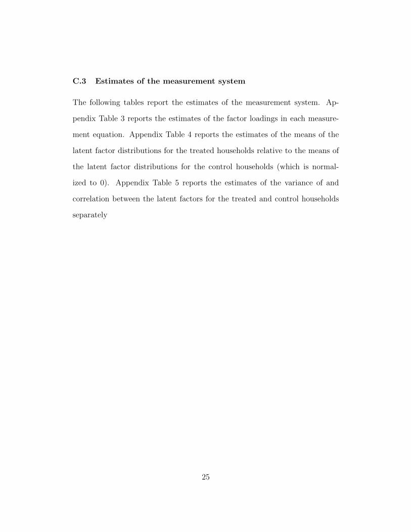
C.3 Estimates of the measurement system

The following tables report the estimates of the measurement system. Ap-

pendix Table 3 reports the estimates of the factor loadings in each measure-

ment equation. Appendix Table 4 reports the estimates of the means of the

latent factor distributions for the treated households relative to the means of

the latent factor distributions for the control households (which is normal-

ized to 0). Appendix Table 5 reports the estimates of the variance of and

correlation between the latent factors for the treated and control households

separately

25

Tab

leA

3:E

stim

ates

offa

ctor

load

ings

inth

em

easu

rem

ent

syst

em

Mea

sure

s:

Ch

ild

's c

og

nit

ive

skil

ls (

t+1

)

Ch

ild

's c

og

nit

ive

Ski

ll (

t)

Ch

ild

's s

oci

o-

emo

tio

na

l sk

ill

(t+

1)

Ch

ild

's s

oci

o-

emo

tio

na

l sk

ill

(t)

Ma

teri

al

inve

stm

ent

Tim

e in

vest

men

tM

oth

er's

cog

nit

ive

skil

l

Mo

ther

's s

oci

o-

emo

tio

na

l sk

ill

Wea

lth

(t)

Bay

ley C

ogn

itiv

e 1

.00

00

00

00

00

0

Bay

ley R

ecep

tive

Lan

gu

age

0.9

20

00

00

00

00

Bay

ley E

xp

ress

ive

Lan

gu

age

1.0

48

00

00

00

00

Bay

ley F

ine

Mo

tor

0.7

68

00

00

00

00

Mac

Art

hu

r-B

ates

Vo

cab

ula

ry

0.7

35

00

00

00

00

Mac

Art

hu

r-B

ates

Co

mp

lex

Sen

ten

ces

0.5

69

00

00

00

00

Bay

ley C

ogn

itiv

e0

1.0

00

00

00

00

0

Bay

ley R

ecep

tive

Lan

gu

age

01

.03

10

00

00

00

Bay

ley E

xp

ress

ive

Lan

gu

age

01

.05

60

00

00

00

Bay

ley F

ine

Mo

tor

00

.95

30

00

00

00

Mac

Art

hu

r-B

ates

Vo

cab

ula

ry0

0.5

76

00

00

00

0

Bat

es D

iffi

cult

su

b-s

cale

(-)

00

1.0

00

00

00

00

Bat

es U

nso

ciab

le s

ub

-sca

le (

-)0

00

.44

40

00

00

0

Bat

es U

nst

op

pab

le s

ub

-sca

le (

-)0

00

.94

80

00

00

0

Ro

thb

art

Inh

ibit

ory

Co

ntr

ol

sub

-sca

le0

01

.00

70

00

00

0

Ro

thb

art

Att

enti

on

su

b-s

cale

00

0.5

05

00

00

00

Bat

es D

iffi

cult

fac

tor

(-)

00

01

.00

00

00

00

Bat

es U

nso

ciab

le f

acto

r (-

)0

00

0.4

39

00

00

0

Bat

es U

nad

apta

ble

(-)

00

00

.63

90

00

00

Bat

es U

nst

op

pab

le (

-)0

00

0.5

11

00

00

0

Nu

mb

er o

f d

iffe

ren

t p

lay m

ater

ials

0

00

01

.00

00

00

0

Nu

mb

er o

f co

lou

rin

g b

oo

ks

00

00

0.3

68

00

00

Nu

mb

er o

f to

ys

bo

ugh

t0

00

00

.58

20

00

0

Nu

mb

er o

f to

ys

that

req

uir

e m

ovem

ent

00

00

0.6

51

00

00

Nu

mb

er o

f to

ys

to l

earn

sh

apes

0

00

00

.74

90

00

0

Nu

mb

er o

f d

iffe

ren

t p

lay a

ctiv

itie

s 0

00

00

1.0

00

00

0

Tim

es t

old

a s

tory

to

ch

ild

in

las

t 3

day

s 0

00

00

0.6

27

00

0

Tim

es r

ead

to

ch

ild

in

las

t 3

day

s 0

00

00

0.7

07

00

0

Tim

es p

layed

wit

h c

hil

d a

nd

to

ys

in l

ast

3 d

ays

00

00

00

.59

70

00

Tim

es l

abel

led

th

ings

to c

hil

d i

n l

ast

3 d

ays

00

00

00

.60

60

00

Mo

ther

s' y

ears

of

edu

cati

on

00

00

00

1.0

00

00

Mo

ther

's v

oca

bu

lary

0

00

00

01

.04

90

0

Nu

mb

er o

f b

oo

ks

for

adu

lts

in t

he

ho

use

00

00

00

0.7

37

00

Nu

mb

er o

f m

agaz

ines

an

d n

ewsp

aper

s 0

00

00

00

.46

10

0

Rav

en's

sco

re (

"IQ

")

00

00

00

0.8

90

00

Did

yo

u f

eel

dep

ress

ed?

(-)

00

00

00

01

.00

00

Bo

ther

ed b

y w

hat

usu

ally

do

n't

bo

ther

yo

u?

(-)

00

00

00

00

.84

20

Had

tro

ub

le k

eep

ing m

ind

on

do

ing?

(-)

00

00

00

00

.91

70

Fel

t ev

eryth

ing y

ou

did

was

an

eff

ort

? (-

)0

00

00

00

0.8

23

0

Did

yo

u f

eel

fear

ful?

(-)

00

00

00

00

.69

50

Did

yo

u s

leep

was

res

tles

s? (

-)0

00

00

00

0.7

98

0

Did

yo

u f

eel

hap

py?

(-)

00

00

00

00

.49

70

Ho

w o

ften

did

yo

u f

eel

lon

ely l

ast

wee

k?

(-)

00

00

00

00

.82

50

Did

yo

u f

eel

yo

u c

ou

ldn

't get

go

ing?

(-)

00

00

00

00

.96

10

Ow

ns

a fr

idge

00

00

00

00

1

Ow

ns

a ca

r 0

00

00

00

00

.37

8

Ow

ns

a co

mp

ute

r 0

00

00

00

00

.94

5

Ow

ns

a b

len

der

00

00

00

00

0.8

36

Ow

n a

was

hin

g m

ach

ing

00

00

00

00

0.4

20

Ow

ns

dw

elli

ng

00

00

00

00

0.5

15

Ow

ns

a ra

dio

0

00

00

00

00

.53

5

Ow

s a

TV

0

00

00

00

00

.91

9

Lat

ent

fact

ors

26

Table A4: Estimates of the difference in means of the latent factors betweentreated and controls

Latent factor Mean Standard

deviation

90% Confidence

Internal

Child's cognitive skills at t+1 0.108 (0.055) [0.015,0.186]

Child's cognitive skills at t -0.031 (0.074) [-0.159,0.084]

Child's socio-emotional skills at t+1 0.082 (0.044) [0.008,0.149]

Child's socio-emotional skills at t 0.037 (0.068) [-0.077,0.148]

Material investments at t+1 0.200 (0.072) [0.072,0.303]

Time investments at t+1 0.345 (0.071) [0.221,0.449]

Mother's cognitive skills -0.026 (0.046) [-0.104,0.047]

Mother's socio-emotional skills 0.007 (0.038) [-0.063,0.063]

Notes: Standard errors in parentheses and 90% confidence intervals in brackets based on1000 bootstraps.

27

Tab

leA

5:E

stim

ates

ofth

eco

rrel

atio

nm

atri

xof

the

late

nt

fact

ors

for

trea

ted

and

contr

ols

Chil

d's

cognit

ive

skil

ls (

t+1

)

Chil

d's

cognit

ive

Skil

l (t

)

Chil

d's

so

cio

-

emo

tio

nal

skil

l (t

+1

)

Chil

d's

so

cio

-

emo

tio

nal

skil

l (t

)

Mat

eria

l

inves

tmen

t

Tim

e

inves

tmen

t

Mo

ther

's

cognit

ive

skil

l

Mo

ther

's

soci

o-

emo

tio

nal

skil

l

Wea

lth (

t)

Chil

d's

co

gnit

ive

skil

ls a

t t+

11

.00

0.6

40

.35

0.3

00

.40

0.2

80

.50

0.1

30

.24

Chil

d's

co

gnit

ive

skil

ls a

t t

0.6

41

.00

0.2

70

.26

0.2

80

.24

0.3

50

.08

0.1

7

Chil

d's

so

cio

-em

oti

onal

skil

ls a

t t+

10

.35

0.2

71

.00

0.6

20

.36

0.2

80

.29

0.1

40

.12

Chil

d's

so

cio

-em

oti

onal

skil

ls a

t t

0.3

00

.26

0.6

21

.00

0.3

20

.26

0.4

40

.16

0.2

4

Mat

eria

l in

ves

tmen

ts a

t t+

10

.40

0.2

80

.36

0.3

21

.00

0.6

20

.61

0.0

70

.32

Tim

e in

ves

tmen

ts a

t t+

10

.28

0.2

40

.28

0.2

60

.62

1.0

00

.41

-0.0

20

.18

Mo

ther

's c

ognit

ive

skil

ls

0.5

00

.35

0.2

90

.44

0.6

10

.41

1.0

00

.19

0.4

4

Mo

ther

's s

oci

o-e

mo

tio

nal

skil

ls

0.1

30

.08

0.1

40

.16

0.0

7-0

.02

0.1

91

.00

0.0

2

Wea

lth a

t t

0.2

40

.17

0.1

20

.24

0.3

20

.18

0.4

40

.02

1.0

0

Chil

d's

co

gnit

ive

skil

ls a

t t+

11

.00

0.6

80

.32

0.2

10

.30

0.1

70

.27

0.1

20

.14

Chil

d's

co

gnit

ive

skil

ls a

t t

0.6

81

.00

0.2

60

.22

0.2

40

.14

0.2

10

.08

0.0

9

Chil

d's

so

cio

-em

oti

onal

skil

ls a

t t+

10

.32

0.2

61

.00

0.4

30

.29

0.2

80

.24

0.1

30

.08

Chil

d's

so

cio

-em

oti

onal

skil

ls a

t t

0.2

10

.22

0.4

31

.00

0.1

00

.05

0.2

90

.15

0.2

4

Mat

eria

l in

ves

tmen

ts a

t t+

10

.30

0.2

40

.29

0.1

01

.00

0.4

50

.48

0.0

30

.26

Tim

e in

ves

tmen

ts a

t t+

10

.17

0.1

40

.28

0.0

50

.45

1.0

00

.29

-0.1

40

.02

Mo

ther

's c

ognit

ive

skil

ls

0.2

70

.21

0.2

40

.29

0.4

80

.29

1.0

00

.12

0.4

0

Mo

ther

's s

oci

o-e

mo

tio

nal

skil

ls

0.1

20

.08

0.1

30

.15

0.0

3-0

.14

0.1

21

.00

0.1

8

Wea

lth a

t t

0.1

40

.09

0.0

80

.24

0.2

60

.02

0.4

00

.18

1.0

0

Co

ntr

ol

gro

up

Tre

ate

d g

rou

p

28

D Specification and robustness checks

In this section of the appendix, we report results associated with specification

and robustness checks we discuss in the main text.

Tables A6 and A7 report the estimates of the investment function and

production functions when the investment function is fully interacted with the

treatment indicator.

Tables A8 and A9 report the estimates of the CES production function

for cognitive skills and socio-emotional skills, respectively, where all the share

parameters (as well as the total productivity factor A) is interacted with the

treatment.

Tables A10 and A11 report the estimates of the CES production function

for cognitive skills and socio-emotional skills, respectively where the child’s age

at follow-up is allowed to determine investments (in the investment functions)

and to affect total-factor productivity.

29

Tab

leA

6:E

stim

ates

ofth

efu

lly

inte

ract

edlo

g-linea

rin

vest

men

tfu

nct

ion

Ma

in e

ffec

tIn

tera

ctio

n w

ith

Tre

atm

ent

Ma

in e

ffec

tIn

tera

ctio

n w

ith

Tre

atm

ent

Co

nst

ant

-0.0

06

-0.0

01

0.2

57

0.3

43

(0.0

20

)(0

.02

7)

(0.0

82

)(0

.07

5)

[-0

.03

,0.0

35

][-

0.0

33

,0.0

53

][0

.11

3,0

.38

9]

[0.2

02

,0.4

45

]

Lo

g o

f ch

ild

's c

ogn

itiv

e sk

ills

at

t0.0

83

0.1

24

0.0

89

-0.0

15

(0.0

84

)(0

.06

1)

(0.1

22

)(0

.10

6)

[-0

.04

1,0

.23

6]

[0.0

15

,0.2

16

][-

0.1

3,0

.24

9]

[-0

.18

6,0

.16

]

Lo

g o

f ch

ild

's s

oci

o-e

mo

tio

nal

skil

ls a

t t

0.0

68

0.1

29

-0.1

58

-0.1

63

(0.0

95

)(0

.10

0)

(0.1

27

)(0

.13

9)

[-0

.06

3,0

.24

5]

[0.0

01

,0.3

23

][-

0.3

94

,0.0

19

][-

0.4

43

,0.0

12

]

Lo

g o

f m

oth

er's

co

gn

itiv

e sk

ills

0.7

53

0.3

64

-0.1

45

0.0

76

(0.1

14

)(0

.12

4)

(0.1

72

)(0

.16

3)

[0.5

63

,0.9

2]

[0.1

55

,0.5

67

][-

0.3

86

,0.1

65

][-

0.1

93

,0.3

46

]

Lo

g o

f m

oth

er's

so

cio

-em

oti

on

al s

kil

ls-0

.092

-0.2

16

-0.0

89

-0.1

30

(0.1

23

)(0

.11

6)

(0.1

56

)(0

.15

7)

[-0

.34

3,0

.05

3]

[-0

.41

9,-

0.0

34

][-

0.2

47

,0.2

46

][-

0.3

66

,0.1

56

]

Lo

g o

f w

ealt

h a

t t

0.0

43

-0.0

53

0.1

16

-0.0

32

(0.1

03

)(0

.14

7)

(0.1

47

)(0

.18

6)

[-0

.13

5,0

.20

8]

[-0

.34

3,0

.15

][-

0.0

97

,0.3

73

][-

0.2

66

,0.3

37

]

Mo

ther

is

mar

ried

at

t+1

0.1

13

0.0

82

0.0

15

0.0

57

(0.0

37

)(0

.03

1)

(0.0

54

)(0

.05

3)

[0.0

53

,0.1

74

][0

.02

7,0

.13

2]

[-0

.07

5,0

.10

5]

[-0

.02

8,0

.14

7]

Lo

g o

f n

um

ber

of

chil

dre

n a

t t+

1-0

.058

-0.1

43

-0.0

62

0.0

74

(0.0

46

)(0

.04

6)

(0.0

73

)(0

.06

9)

[-0

.14

8,0

][-

0.2

21

,-0

.07

1]

[-0

.16

,0.0

78

][-

0.0

24

,0.1

99

]

Lo

g o

f av

erag

e m

ale

wag

es i

n v

illa

ge

at t

+1

0.0

07

0.0

87

0.0

84

-0.1

91

(0.0

73

)(0

.07

7)

(0.0

97

)(0

.10

0)

[-0

.13

1,0

.10

5]

[-0

.03

8,0

.20

9]

[-0

.07

1,0

.24

5]

[-0

.36

8,-

0.0

47

]

Lo

g o

f av

erag

e fe

mal

e w

ages

in

vil

lage

at t

+1

0.0

14

-0.0

10

-0.0

18

0.0

79

(0.0

66

)(0

.07

2)

(0.0

84

)(0

.09

1)

[-0

.07

9,0

.13

6]

[-0

.14

5,0

.09

4]

[-0

.19

1,0

.09

1]

[-0

.04

6,0

.24

5]

Lo

g o

f m

ater

ial

inves

tmen

tL

og o

f ti

me

inves

tmen

t

Not

es:

Sta

nd

ard

erro

rsin

par

enth

eses

and

90%

con

fid

ence

inte

rvals

inb

rack

ets

base

don

1000

boots

trap

s.

30

Table A7: Estimates of the CES production for cognitive and socio-emotionalskills with a fully interacted log-linear investment function

Cognitive

skills

Socio-emotional

skills

Child's cognitive skills at t 0.567 0.104

(0.051) (0.054)

[0.499,0.667] [0.012,0.189]

Child's socio-emotional skills at t 0.037 0.416

(0.046) (0.057)

[-0.035,0.118] [0.355,0.532]

Mother's cognitive skills 0.053 0.017

(0.104) (0.120)

[-0.122,0.235] [-0.254,0.136]

Mother's socio-emotional skills 0.052 0.155

(0.047) (0.057)

[-0.023,0.123] [0.043,0.229]

Material investments at t+1 0.358 -0.155

(0.141) (0.150)

[0.1,0.551] [-0.278,0.211]

Time investments at t+1 -0.114 0.384

(0.107) (0.108)

[-0.292,0.061] [0.158,0.511]

Number of children in household at t+1 0.047 0.078

(0.029) (0.027)

[-0.002,0.092] [0.028,0.119]

Control function for material investments -0.298 0.317

(0.160) (0.161)

[-0.532,-0.001] [-0.051,0.459]

Control function for time investment 0.137 -0.3

(0.126) (0.118)

[-0.07,0.333] [-0.461,-0.079]

Complementarity parameter 0.08 0.011

(0.065) (0.058)

[-0.031,0.179] [-0.067,0.122]

Elasticity of substitution 1.087 1.012

(0.077) (0.065)

[0.97,1.218] [0.938,1.139]

Productivity parameter (A) 0.991 0.993

(0.012) (0.013)

[0.968,1.007] [0.974,1.015]

Productivity parameter interacted with treatment 0.08 -0.037

(0.066) (0.053)

[-0.009,0.206] [-0.13,0.041]

Notes: Standard errors in parentheses and 90% confidence intervals in brackets based on1000 bootstraps.

Table A8: Estimates of the CES production for cognitive skills where all theshare parameters are interacted with the treatment

Without control

function

With control

function

Child's cognitive skills at t 0.548 0.524

(0.063) (0.071)

[0.455,0.665] [0.435,0.665]

Child's cognitive skills at t * Treat 0.072 0.064

0.088 0.088

[-0.068,0.221] [-0.078,0.211]

Child's socio-emotional skills at t 0.02 0.033

(0.064) (0.071)

[-0.078,0.14] [-0.068,0.164]

Child's socio-emotional skills at t * Treat 0 -0.005

0.084 0.085

[-0.142,0.128] [-0.147,0.128]

Mother's cognitive skills 0.281 0.125

(0.085) (0.173)

[0.16,0.429] [-0.151,0.416]

Mother's cognitive skills * Treat -0.172 -0.151

0.108 0.112

[-0.371,-0.023] [-0.351,0.011]

Mother's socio-emotional skills 0.042 0.042

(0.079) (0.076)

[-0.111,0.142] [-0.106,0.147]

Mother's socio-emotional skills * Treat 0.054 0.04

0.095 0.094

[-0.088,0.224] [-0.103,0.21]

Material investments at t+1 0.082 0.375

(0.063) (0.236)

[-0.023,0.19] [0.039,0.782]

Material investments at t+1 *Treat 0.011 0.001

0.078 0.08

[-0.121,0.135] [-0.137,0.125]

Time investments at t+1 0 -0.141

(0.062) (0.153)

[-0.12,0.082] [-0.454,0.031]

Time investments at t+1 * Treat 0.015 0.029

0.076 0.077

[-0.098,0.152] [-0.082,0.17]

Number of children in household at t+1 0.026 0.041

(0.042) (0.044)

[-0.045,0.094] [-0.033,0.112]

Number of children in household at t+1 * Treat 0.047 0.062

0.033 0.036

[-0.008,0.094] [-0.002,0.116]

32

Table A8 : Estimates of the CES production for cognitive skills where all theshare parameters are interacted with the treatment (continued)

Without control

function

With control

function

Control function for material investments - -0.3

0.229

[-0.692,0.02]

Control function for time investment - 0.14

0.15

[-0.048,0.434]

Complementarity parameter 0.143 0.057

0.081 0.061

[-0.035,0.229] [-0.018,0.169]

Elasticity of substitution 1.166 1.061

0.105 0.073

[0.966,1.297] [0.982,1.203]

Productivity parameter (A) 0.978 0.987

0.012 0.011

[0.966,1.005] [0.97,1.007]

Productivity parameter interacted with treatment 0.097 0.08

0.054 0.075

[0.016,0.189] [-0.018,0.224]

Notes:

Standard errors in parentheses and 90% confidence intervals in brackets based on 1000 boot-

straps.

33

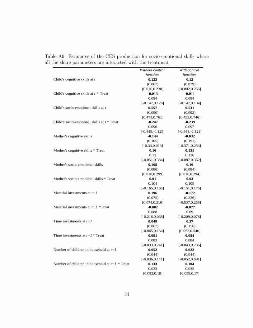
Table A9: Estimates of the CES production for socio-emotional skills whereall the share parameters are interacted with the treatment

Without control

function

With control

function

Child's cognitive skills at t 0.123 0.12

(0.067) (0.079)

[0.016,0.238] [-0.002,0.256]

Child's cognitive skills at t * Treat -0.013 -0.011

0.084 0.084

[-0.147,0.126] [-0.147,0.134]

Child's socio-emotional skills at t 0.557 0.531

(0.090) (0.092)

[0.473,0.761] [0.453,0.746]

Child's socio-emotional skills at t * Treat -0.247 -0.239

0.096 0.097

[-0.449,-0.125] [-0.441,-0.121]

Mother's cognitive skills -0.144 -0.032

(0.105) (0.191)

[-0.33,0.013] [-0.371,0.253]

Mother's cognitive skills * Treat 0.16 0.131

0.13 0.136

[-0.051,0.384] [-0.087,0.362]

Mother's socio-emotional skills 0.168 0.16

(0.086) (0.084)

[0.018,0.299] [0.016,0.294]

Mother's socio-emotional skills * Treat 0.01 0.03

0.104 0.105

[-0.165,0.165] [-0.151,0.175]

Material investments at t+1 0.196 -0.172

(0.075) (0.236)

[0.074,0.316] [-0.537,0.258]

Material investments at t+1 *Treat -0.082 -0.077

0.088 0.09

[-0.216,0.068] [-0.209,0.078]

Time investments at t+1 0.048 0.37

(0.067) (0.156)

[-0.065,0.154] [0.052,0.546]

Time investments at t+1 * Treat 0.091 0.084

0.083 0.084

[-0.033,0.241] [-0.043,0.236]

Number of children in household at t+1 0.052 0.022

(0.044) (0.044)

[-0.036,0.111] [-0.052,0.091]

Number of children in household at t+1 * Treat 0.133 0.104

0.033 0.035

[0.082,0.19] [0.059,0.17]

34

Table A9 (cont.): Estimates of the CES production for socio-emotional skillswhere all the share parameters are interacted with the treatment

Without control

function

With control

function

Control function for material investments - 0.379

(0.223)

[-0.038,0.724]

Control function for time investment - -0.34

(0.145)

[-0.496,-0.033]

Complementarity parameter -0.023 -0.042

(0.069) (0.051)

[-0.118,0.102] [-0.101,0.06]

Elasticity of substitution 0.977 0.959

(0.069) (0.050)

[0.895,1.114] [0.908,1.064]

Productivity parameter (A) 1.017 1.021

(0.012) (0.009)

[0.981,1.019] [0.987,1.017]

Productivity parameter interacted with treatment -0.027 -0.056

0.039 0.057

[-0.082,0.046] [-0.118,0.061]

Notes: Standard errors in parentheses and 90% confidence intervals in brackets based on

1000 bootstraps.

35

Table A10: Estimates of the CES production for cognitive skills, where age isallowed to affect total-factor productivity

Without control

function

With control

function

Child's cognitive skills at t 0.593 0.565

(0.044) (0.057)

[0.524,0.67] [0.485,0.677]

Child's socio-emotional skills at t 0.032 0.038

(0.043) (0.050)

[-0.037,0.106] [-0.033,0.125]

Mother's cognitive skills 0.179 0.018

(0.049) (0.127)

[0.103,0.263] [-0.176,0.231]

Mother's socio-emotional skills 0.066 0.055

(0.045) (0.049)

[-0.011,0.131] [-0.026,0.125]

Material investments at t+1 0.09 0.418

(0.033) (0.207)

[0.034,0.145] [0.095,0.744]

Time investments at t+1 0.006 -0.145

(0.035) (0.141)

[-0.055,0.059] [-0.392,0.047]

Number of children in household at t+1 0.034 0.051

(0.026) (0.030)

[-0.009,0.078] [0.001,0.098]

Control function for material investments - -0.344

(0.217)

[-0.673,-0.006]

Control function for time investment - 0.16

(0.150)

[-0.053,0.421]

Complementarity parameter 0.149 0.056

(0.079) (0.061)

[-0.031,0.229] [-0.036,0.164]

Elasticity of substitution 1.175 1.059

(0.101) (0.071)

[0.97,1.296] [0.965,1.196]

Productivity parameter (A) 0.984 0.998

(0.018) (0.016)

[0.958,1.014] [0.968,1.023]

Productivity parameter interacted with treatment 0.091 0.07

0.053 0.073

[0.029,0.201] [-0.013,0.223]

Productivity parameter interacted with age 0 -0.005

(0.008) (0.007)

[-0.011,0.014] [-0.013,0.009]

Notes: Standard errors in parentheses and 90% confidence intervals in brackets based on1000 bootstraps.

Table A11: Estimates of the CES production for socio-emotional skills, whereage is allowed to affect total-factor productivity

Without control

function

With control

function

Child's cognitive skills at t 0.112 0.116

(0.044) (0.059)

[0.04,0.188] [0.025,0.218]

Child's socio-emotional skills at t 0.443 0.428

(0.054) (0.057)

[0.368,0.551] [0.349,0.538]

Mother's cognitive skills -0.055 0.057

(0.065) (0.138)

[-0.166,0.046] [-0.169,0.281]

Mother's socio-emotional skills 0.146 0.155

(0.057) (0.057)

[0.05,0.23] [0.046,0.231]

Material investments at t+1 0.148 -0.22

(0.042) (0.192)

[0.08,0.218] [-0.526,0.091]

Time investments at t+1 0.112 0.398

(0.041) (0.131)

[0.046,0.181] [0.174,0.597]

Number of children in household at t+1 0.093 0.065

(0.026) (0.027)

[0.049,0.135] [0.027,0.115]

Control function for material investments - 0.385

(0.198)

[0.061,0.703]

Control function for time investment - -0.31

(0.135)

[-0.505,-0.064]

Complementarity parameter 0.061 0.029

(0.075) (0.055)

[-0.084,0.151] [-0.049,0.116]

Elasticity of substitution 1.065 1.029

(0.086) (0.060)

[0.923,1.178] [0.953,1.131]

Productivity parameter (A) 0.992 0.996

(0.020) (0.018)

[0.965,1.031] [0.963,1.022]

Productivity parameter interacted with treatment -0.027 -0.042

0.041 0.057

[-0.081,0.056] [-0.113,0.071]

Productivity parameter interacted with age -0.002 0.004

(0.007) (0.008)

[-0.013,0.009] [-0.01,0.017]

Notes: Standard errors in parentheses and 90% confidence intervals in brackets based on1000 bootstraps.

References

Andresen, E., J. Malmgren, W. Carter, and D. Patrick (1994). Screening fordepression in well older adults: evaluation of a short form of the ces-d (centerfor epidemiologic studies depression scale). American Journal of PreventiveMedicine 10 (758), 77–84.

Attanasio, O., C. Fernandez, E. Fitzsimons, S. Grantham-McGregor,C. Meghir, and M. Rubio-Codina (2014). Using the infrastucture of a Condi-tional Cash Transfer programme to deliver a scalable integrated early childdevelopment programme in Colombia: A cluster randomised controlled trial.Forthcoming in British Medical Journal 349, g5785.

Bates, J., C. Freeland, and M. Lounsbury (1979). Measurement of infantdifficultness. Child Development 50, 794–803.

Bayley, N. (2006). Bayley Scales of Infant and Toddler Development (3rd ed.).San Antonio, TX: Harcourt Assessment.

Caldwell, B. and R. Bradley (2001). HOME Inventory and AdministrationManual (Third Edition ed.). Little Rock, AK: University of Arkansas forMedical Sciences.

Cattell, R. (1966). The scree test for the number of factors. MultivariateBehavioral Research 1, 629–637.

Dunnn, L., E. Padilla, D. Lugo, and L. Dunn (1986). Manual del Exam-inador para el Test de Vocabulario en Imgenes Peabody (Peabody PictureVocabulary Test), Adaptacin Hipanoamericana (Hispanic-American Adap-tion). Minneapolis, MS: Pearson Assessments.

Fernald, L., P. Kariger, P. Engle, and A. Raikes (2009). Examining child de-velopment in low-income countries: A toolkit for the assessment of childrenin the first five years of life. Washington DC: The World Bank.

Frongillo, E., S. Sywulka, and P. Kariger (2003). UNICEF psychosocial careindicators project. Final report to UNICEF. Mimeo, Cornell University.

Gonzalez, V., A. Stewart, P. Ritter, and K. Lorig (1995). Translation andvalidation of arthritis outcome measures into Spanish. Arthritis Rheum 38,1429–46.

Gorusch, R. (1983). Factor Analysis. Hillsdale, NJ: Lawrence Erlbaum Asso-ciates.

38

Gorusch, R. (2003). Factor analysis. In Handbook of psychology: Researchmethods in psychology, Volume 2, pp. 143–164. Hoboken, NJ: John Wiely &Sons, Inc.

Hamadani, J., F. Tofail, A. Hilaly, S. Huda, P. Engel, and S. Grantham-McGregor (2010). Use of Family Care Indicators and their relationshipwith child development in bangladesh. Journal of Health Population andNutrition 28 (1), 23–33.

Horn, J. (1965). A rationale and a test for the number of factors in factoranalysis. Psychometrika 30, 179–185.

Jackson-Maldonado, D. (2011). Spanish cdi-iii development and preliminaryresults. Presentation at the International Congress for the Study of ChildLanguage, Montreal.

Jackson-Maldonado, D. and B. Conboy (2011). Preliminary norms and validityfor the Spanish CDI-III. American Speech-Language-Hearing Association(ASHA) Annual Conference. San Diego, CA.

Jackson-Maldonado, D., V. Marchman, and L. Fernald (2012). Short formversions of the Spanish MacArthur-Bates Communicative Development In-ventories. In Applied Psycholinguistics. Cambridge: Cambridge UniversityPress.

Jackson-Maldonado, D., D. Thal, V. Marchman, T. Newton, L. Fenson, andB. Conboy (2003). MacArthur Inventarios del Desarrollo de Habilidades Co-municativas: User’s guide and technical manual. Baltimore, MD: Brookes.

Kaiser, H. (1960). The application of electronic computers to factor analysis.Educational and Psychological Measurement 20, 141–151.

Putnam, S. P., M. Gartstein, and M. K. Rothbart (2006). Measurement offine-grained aspects of toddler temperament: The Early Childhood BehaviorQuestionnaire. Infant Behavior and Development 29 (3), 386–401.

Putnam, S. P., J. Jacobs, M. Garstein, and M. Rothbart (2010). Develop-ment and assessment of short and very short forms of the Early ChildhoodBehavior Questionnaire.

Radloff, L. (1977). The CES-D scale: A self-report depression scale for researchin the general population. Applied Psychological Measurement 1 (3), 385–401.

39

Raven, J. (1981). Manual for Raven’s progressive matrices and vocabularyscales. In Research Supplement No.1: The 1979 British Standardisation ofthe Standard Progressive Matrices and Mill Hill Vocabulary Scales, TogetherWith Comparative Data From Earlier Studies in the UK, US, Canada, Ger-many and Ireland. San Antonio, TX: Harcourt Assessment.

Velicer, W. (1976). Determining the number of components from the matrixof partial correlations. Psychometrika 41, 32l–327.

40