estimating the spatial distribution of snow in mountain basins using remote sensing and energy

WATER RESOURCES RESEARCH, VOL. 34, NO. 5, PAGES 1275-1285, MAY 1998

Estimating the spatial distribution of snow in mountain basins using remote sensing and energy balance modeling Donald W. Cline

National Operational Hydrologic Remote Sensing Center, Office of Hydrology, National Weather Service, Chanhassen, Minnesota

Roger C. Bales Department of Hydrology and Water Resources, University of Arizona, Tucson

Jeff Dozier

Donald Bren School of Environmental Science and Management, University of California, Santa Barbara

Abstract. We present a modeling approach that couples information about snow cover duration from remote sensing with a distributed energy balance model to calculate the spatial distribution of snow water equivalence (SWE) in a 1.2 km 2 mountain basin at the peak of the accumulation season. In situ measurements of incident solar radiation, incident longwave radiation, air temperature, relative humidity, and wind speed were distributed around the basin on the basis of topography. Snow surface albedo was assumed to be spatially constant and to decrease with time. Distributed snow surface temperature was estimated as a function of modeled air temperature. We computed the energy balance for each pixel at hourly intervals using the estimated radiative fluxes and bulk-aerodynamic turbulent-energy flux algorithms from a snowpack energy and mass balance model. Fractional snow cover within each pixel was estimated from three multispectral images (Landsat thematic mapper), one at peak accumulation and two during snowmelt, using decision trees and a spectral mixture model; from these we computed snow cover duration at subpixel resolution. The total cumulative energy for snowmelt at each remote sensing date was weighted by the fraction of each pixel's area that lost its snow cover by that date to determine an initial SWE for each pixel. We tested the modeling approach in the well-studied Emerald Lake basin in the southern Sierra Nevada. With no parameter fitting the modeled spatial pattern of SWE and the mean basin SWE agreed with intensive field survey data. As the modeling approach requires only a remote sensing time series and an ability to estimate the energy balance over the model domain, it should prove useful for computing SWE distributions at peak accumulation over larger areas, where extensive field measurements of SWE are not practical.

1. Introduction

Seasonally snow-covered areas of the Earth's mountain ranges account for the major source of the water supply for runoff and groundwater recharge over wide areas of the mid- latitudes. In these areas the total downstream water yield from mountain basins is directly proportional to the mountain snowpack and can be predicted with reasonable success using simple empirical indices that have not changed significantly in four decades [Elder et al., !991b]. While empirical snowmelt runoff models have traditionally been useful for operational runoff volume forecasts, they provide little information on the timing, rate, or magnitude of discharge, and they are inappropriate in situations outside the boundary conditions governing the development of the relevant empirical parameters. Thus they may fail to adequately predict water yield in extreme or un- usual years and cannot be reliably used in investigations examining snowmelt responses to climate variability and change. Copyright 1998 by the American Geophysical Union.

Paper number 97WR03755. 0043-1397/98/97WR-03755509.00

These problems, and the increasing importance of understand- ing intrabasin snowmelt for environmental analysis of such factors as basin ecology [Baron et al., 1993], water chemistry [Wolford et al., 1996] and hillslope erosion [Tarboton et al., 1991], have motivated the recent development of physically based, spatially distributed snowmelt models. Such models require information on the spatial distribution of snowpack water storage. But mountain snowpacks are spatially heterøge - nous, reflecting the influences of rugged topography on precipitation, wind redistribution of snow, and surface energy fluxes during the accumulation season [Elder et al., 1991b], and no widely suitable method yet exists to directly map SWE in rugged mountain regions. One of the main obstacles to physically based modeling is the accumulation of the necessary meteorological and snow cover data to run, calibrate, and validate such models [Bales and Harrington, 1995]. This paper directly addresses this obstacle.

The spatial distribution of snow cover can be measured from many operational remote sensing platforms, and recent algorithm developments even permit the determination of subpixel fraction of snow cover [Rosenthal and Dozier, 1996]. However,

1275

1276 CLINE ET AL.: ESTIMATING THE SPATIAL DISTRIBUTION OF SNOW

California, USA 42

Emerald Lake

28

met station

.. .

N 1 km Contour interval 25 rn

Figure 1. Map of study area.

direct measurement of SWE by remote sensing is not yet feasible. At present, therefore, the measurement of the spatial distribution of SWE and total snow volume within a basin must be performed by intensive field sampling to capture the large spatial variability of mountain snowpacks. Logistical and safety limitations gener- ally restrict the number of field samples that may be so obtained [Elder et al., 1991b]. Thus the problem of determining the volume and distribution of snowpack water storage within mountain basins remains acute. In this paper we address this problem with a 'model to recover, later in the season, the spatial distribution of SWE in mountain basins at the onset of snowmelt.

The duration (D) of snow cover at any given location may be viewed as a function of the original quantity of SWE at that location at the onset of snowmelt (SWEi) and the energy exchanges (E) at that location over time. If D and E can be determined, this conceptual model can be inverted to calculate the initial spatial distribution of SWE:

SWEi = f(D, E)

This conceptual "snow cover depletion" model for estimating SWEi from snow cover duration and snowpack energy exchanges was first presented by Martinec and Rango [1981]. They determined snow cover duration on a 1 x 1 km grid by visually inter- preting snow cover within each 1 knl 2 grid cell using a time series of Landsat data, and they employed a simple empirical degree- day approach to represent snowpack energy exchanges. Here we build upon their approach in three ways: (1) We incorporate physically based radiative and turbulent energy balance processes for the determination of snowpack energy exchanges, (2) we employ state-of-the-art snow cover classification techniques for the determination of snow cover duration at subpixel (30 x 30 m) resolution from multispectral image data, and (3) we compare the model results to empirical SWE distribution patterns and total basin water volume determined from intensive field measurements of SWE.

2. Methods

We modeled the spatial distribution of SWE near peak accumulation and the onset of snowmelt of the 1993 water year

at Emerald Lake watershed, a small, high basin in Sequoia National Park, Sierra Nevada, California (Figure 1). The watershed is about 120 ha in area with 636 m relief; Tonnessen [1991] describes it in detail. We selected the site for this study because of previous and ongoing field investigations of the distributions of SWE in the basin [e.g., Elder et al., 1991a, b, 1995] that provided micrometeorological data and facilitated validation of the modeling approach. We determined snow cover duration using a time series of three Landsat thematic mapper (TM) scenes that were available during the snowmelt season. We modeled the energy balance components using micrometeorological data measured near the inlet of Emerald Lake at the base of the watershed (2813 m elevation) and a 30 m resolution gridded digital elevation model (DEM) of the watershed. The overall modeling approach is summarized in Figure 2.

2.1. Snow Cover Depletion

The depletion of snow cover was determined on a subpixel basis using three Landsat TM scenes (April 4, May 5, and June 22, 1993) of the Emerald Lake area. The first scene was near the peak of the accumulation season and the onset of snowmelt. The scenes were classified using decision trees and a spectral mixture model [Rosenthal and Dozier, 1996] (Figure 3). As opposed to the familiar binary snow cover classification where pixels are classified as either "snow" or "no snow," this method yields the fractional snow-covered area within each pixel and helps overcome mixed-pixel and variable-illumina- tion problems that ordinarily complicate snow mapping [e.g., Dozier, !989; Dozier and Marks, 1987; Engman and Gurney, 1991]. This method was found to provide snow classification accuracy equal to that obtainable using high-resolution aerial photography [Rosenthal and Dozier, 1996].

To determine snow cover depletion from a time series of subpixel fractional snow cover, we assumed that the reduction in the fractional snow-covered area over time is spatially co- herent; that is, the extents of a patch of snow in a partially covered pixel may become smaller over time, but snow cover does not otherwise change locations within the pixel. Using this assumption, an area-weighted, or "fractional depletion," of

CLINE ET AL.: ESTIMATING THE SPATIAL DISTRIBUTION OF SNOW 1277

Remote Sensing Time Series

........ to t2

Incident Incident Air Relative Wind Solar Longwave Temperature Humidity Speed

T•tn•ei .•-•. ..-'•• .-.,x•• ..-•• ...... ..-'..•...x.-:••j .-:.,.'. "•• Pixel-by-Pixel ..

Cumulative Energy Available for Snowmelt

.; .-,-x•_•,,:--•x:•: ... t 1 '"..4,•i;::..-.-.: ' .... t 2 ....

Sub-Pixel Snow Cover •me Series SWE Distribution at t O

Figure 2. Flowchart showing modeling structure with three main components: (1) determination of fractional snow cover at subpixel levels using spectral unmixing and decision trees, (2) computation of the energy balance at each pixel using estimated micrometeorological data distributions, and (3) coupling the two to determine the initial SWE at the beginning of the model run at each pixel.

snow cover in each pixel was determined for the date of each TM scene.

For example, consider a pixel with 80% snow cover at the first remote sensing date, corresponding to peak accumulation (Figure 4). The SWE/of 20% of the pixel area is automatically zero. At the second date a reduction in fractional snow cover

from 80% to 50% indicates that the snow cover depletion of an additional 30% of the pixel area is defined by date 2, and snow cover depletion is then defined for 50% of the pixel area. If by the third date the fractional snow cover is reduced further to

10%, then 40% of the pixel area has snow cover depletion defined by date 3, and snow cover depletion for 90% of the pixel area is then defined. One hundred percent of snow cover depletion is defined when all snow in the pixel is gone. This subpixel area-weighting approach permits a more precise def- inition of the duration of snow cover, and subsequently SWE i for each pixel, than would be possible using a binary snow cover classification. In that case it is likely that a pixel would be considered snow-free even when a substantial amount of snow

cover remained in the pixel (e.g., <50%). Thus a binary snow cover classification would tend to underestimate the duration

of snow cover and subsequently SWE/.

2.2:. Meteorological Data Distributions and Energy Budget Computation

Five spatially and temporally varying meteorological variables were used to compute the energy budget throughout the modeling domain: incident solar radiation, incident longwave radiation, air temperature, relative humidity, and wind speed. All variables were modeled on an hourly time step for 1608 hours (67 days) from April 21 through June 29, 1993.

2.2.1. Incident solar radiation. Incident solar-radiation

was spatially distributed using TOPORAD [Dozier and Frew, 1990], an algorithm that accounts for effects of elevation on the optical thickness of the atmosphere and for effects of terrain on shading and radiation reflected from nearby pixels. Total downwelling radiation on a horizontal surface, and the direct and diffuse components, were estimated using a two-stream approximation. Incident solar radiation was modeled sepa-

rately in thirty 0.1 •m spectral bands between 0.3 and 3.0 •m and integrated to determine the total insolation on each pixel. In addition to the digital elevation data, TOPORAD requires a map of surface albedo at each time step and three parameters describing the atmospheric condition: optical depth, single scattering albedo, and the scattering phase function. These factors were modeled using methods described below. Dozier [1980], Dubayah et al. [1990], and Elder et al. [1991a] provide more complete descriptions of the solar radiation algorithms used here.

For the Emerald Lake basin, surface albedo was considered both spatially and temporally constant at 0.6 for purposes of computing terrain reflections in TOPORAD (but not for computing the net shortwave energy flux, discussed below). The required atmospheric parameters are important for TOPORAD to correctly determine the different insolation characteristics between predominantly clear skies and conditions when diffuse irradiance is prevalent, but they are not easily determined from information normally available in remote alpine basins. For each hour of simulation, three parameters were needed for each of the 30 spectral bands modeled. We used LOWTRAN7 [Kneizys et al., 1988] to identify suitable atmospheric parameters for the two-stream model by matching TOPORAD results for the pixel corresponding to the micrometeorological station to field data, similar to the method of Dubayah [1991]. Total atmospheric transmittance (Ts) for each hour of daylight was calculated from measured incident solar radiation. The hourly T s values were grouped into five general categories (Table 1) for simplification. By iteratively varying the meteorological range (i.e., •1.3 x visibility) parameter in LOWTRAN7 (the only parameter that can be modified to alter the atmospheric transmittance in the model for a given clear atmosphere in the absence of atmospheric profile data) and the cloud type parameter, a set of atmospheric parameters was found for each of the five T s categories. The resultant look-up table of five sets of 90 atmospheric parameter values was then called as a function of T s for each hour.


Landsat Image (Band 4) Sub-Pixel Snow Cover Fraction April 4• 1993

, ............ .....,.,.. ß • '•"-* ...... :•-•':;•.,-•.•-'•:•••••2• "•: ' '•< .' '* • J•:;•:•' •' --•>

. ,:•5•:• :. ..... •. 7 . . . •- . .. -: -•.• •..;,•....•.• • •'-•-•' .• .....

•. , • • '• • ,- •-.• •.• •".•:'• ..•-,.• .... •:..•' • .-,..•;.,.-..- .• •; ...,•.-.• :.-,.•..•. W-• •. .•.-. .• •,•..• - .... .;•..

•"• :...;• ........... .•.. •-. . ;" '••A•. ?..•...• ß

May 22, 1993 •,•.•:i:.•-•...i-.•,•i:,•,•;•,':•.."•,.•"..".•,i:"-•..•.•%•.•-•'•-•:." ...• •..%•,,•;•-.. ;•.•.. •--:• •..'..•..::•.-.: •..:-•

ß • •,:.•:•- .. g:•...:•-,-½.•:•"•"•'•'•)• •. .:•:•...? •.,• ...... • ........ ß ............ :•. -•..,•¾•.-.:.-•,.:-,..,.• . ., ..-;...• -.-- .. :- ..... .... ...... • •,•-..•:• .•., ....,.,-•:• ............ • -•;m,:• r•..;•½• •...-,•.• ,.•.-...•>. >.-. •'- •-•-•-m••- -•••••••••••<•.•,•....•: •.,. ',. .... •.. ....'.., .. ½.-.-.,-.?p•:

',.: ß •-: '•9;' '.½• .?•>g ' ." ' ' .. :' ."'.' ".'Z ;' )-'-:'..' .: ß . ß ;..- •.. &..:.•';';• ..... . •: . .•;---.•'.• :. :... . ....,,,..... .... :.:•.•.• •.. ß .•..•:•;½•. -'•. .•.. •,.:•..:.•...

...; •..'•'2;:.

".;;',.;.-...'.'.,'.; ?.. ß '..-,,'.:,...•.,•:•s.:....,,.....,.•....' .;....,::.;• ............ ..,.., ......... ...:.....,... ......... ...... .... ,........... ....... ?.•;.,:?.:...,.,,......,...:½•,•,,,•.•s:..:,,:.:•,•,,.,;,..,.,...,. .... •..

June i: -!

.'i;i• ,.

....

...

1993

Figure 3. Three TM scenes classified for subpixel snow cover fraction. Band 4 of each scene is shown on the left. The classified image is on the right. In the classified image a pure white pixel has a fractional snow cover of 100%, while a pure black pixel has no snow cover. The rectangle shows the boundary of the study area.

2.2.2. Air temperature, relative humidity, and wind speed. In the absence of measured lapse information, hourly air temperatures were simply extrapolated from the station data as a function of elevation, time of day, and insolation using the

30 m DEM. Following Hungerford et al. [1989], we assumed a daytime lapse rate of -0.006øC m -• with a 10% increase during cloudy conditions and 10% decrease during very clear conditions and a nighttime lapse rate of -0.003øC m-•. Their


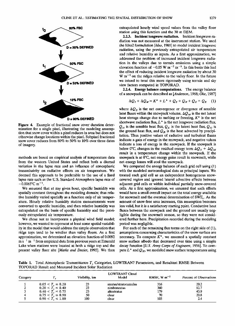
D = 20% DEFINED

tl 50% FSC

t 2

D = 50% DEFINED

10% FSC

D = 90% DEFINED

Figure 4. Example of fractional snow cover duration determination for a single pixel, illustrating the modeling assumption that snow cover within a pixel reduces in area but does not otherwise change locations within the pixel. Subpixel fractional snow cover reduces from 80% to 50% to 10% over three dates

of imagery.

methods are based on empirical analysis of temperature data from the western United States and reflect both a diurnal

variation in the lapse rate and an influence of atmospheric transmissivity on radiative effects on air temperature. We deemed this approach to be preferable to the use of a fixed lapse rate such as the U.S. Standard Atmosphere lapse rate of -0.0065øC m- •.

We assumed that at any given hour, specific humidity was spatially constant throughout the modeling domain; thus relative humidity varied spatially as a function only of air temperature. Hourly relative humidity station measurements were converted to specific humidity, and then relative humidity was extrapolated on the basis of specific humidity and the previously extrapolated air temperature.

We chose not to incorporate a physical wind field model; however, we wanted to represent at least some spatial variability in the model that would address the simple observation that ridge tops tend to be windier than valley floors. As a first approximation, we determined an elevation function of 0.0092 m s- • m- • from empirical data from previous years at Emerald Lake when stations were located at both a ridge top and the present valley floor site [Marks and Dozier, 1992]. We then

extrapolated hourly wind speed values from the valley floor station using this function and the 30 m DEM.

2.2.3. Incident longwave radiation. Incident longwave radiation was not measured at the instrument station. We used

the Idso2 formulation [Idso, 1981] to model incident longwave radiation, using the previously extrapolated air temperature and relative humidity as inputs. As a first approximation, we addressed the problem of increased incident longwave radiation in the valleys due to terrain emissions using a simple elevation function of -0.05 W m -2 m -•. In this basin this had

the effect of reducing incident longwave radiation by about 30 W m -2 on the ridges relative to the valley floor. In the future we intend to treat this more rigorously using terrain and sky view factors computed in TOPORAD.

2.2.4. Energy balance computations. The energy balance of a snowpack can be described as [Anderson, 1968; Oke, 1987]

AQs + AQM= K* + L* + QE + Q•+ QG + QR (1)

where A Qs is the net convergence or divergence of sensible heat fluxes within the snowpack volume, A QM is the net latent heat storage change due to melting or freezing, K* is the net shortwave radiation flux, L * is the net longwave radiation flux, Q•r is the sensible heat flux, Q•r is the latent heat flux, QG is the ground heat flux, and Q R is the heat advected by precipitation. Thus positive values of radiative and turbulent fluxes indicate a gain of energy in the snowpack, and negative values indicate a loss of energy in the snowpack. If the snowpack is below 0øC, changes in the residual energy term AQs + AQM result in a temperature change within the snowpack. If the snowpack is at 0øC, net energy gains result in snowmelt, while net energy losses will cool the snowpack.

We computed the energy balance of each grid cell using (1) with the modeled meteorological data as principal inputs. We treated each grid cell as an independent homogenous snow- covered region and ignored lateral advective effects between adjacent grid cells or within individual partially snow-covered cells. As a first approximation, we assumed that such effects would have a small overall impact on the total energy available for snowmelt and the eventual determination of SWE i. As the amount of snow-free area increases, this assumption becomes less valid, but it is a satisfactory starting point. Conductive heat fluxes between the snowpack and the ground are usually negligible during the snowmelt season, so they were not considered further here. Precipitation recorded during the modeling period was negligible.

For each of the remaining flux terms on the right side of (1), assumptions concerning characteristics of the snow surface are necessary. To compute K*, we assumed a spatially constant snow surface albedo that decreased over time using a simple decay function [U.S. Army Corps of Engineers, 1956]. To compute L * and Q•r, we modeled snow surface temperatures using

Table 1. Total Atmospheric Transmittance T s Categories, LOWTRAN7 Parameters, and Resultant RMSE Between TOPORAD Result and Measured Incident Solar Radiation

LOWTRAN7 Cloud

Category T s Visibility, km Model RMSE, W m -2 Percent of Observations

1 0.05 < T s <- 0.20 23 stratus/stratocumulus 316 20.2 2 0.20 < T s <- 0.40 23 nimbostratus 360 12.7 3 0.40 < T s <_ 0.75 23 altostratus 179 43.9 4 0.75 < T s <- 0.90 50 clear 70 20.8 5 0.90 < Ts <- 1.00 100 clear 105 2.4


SWE, rn

012345

Standard deviations

-3-2-1 0 I 2 3

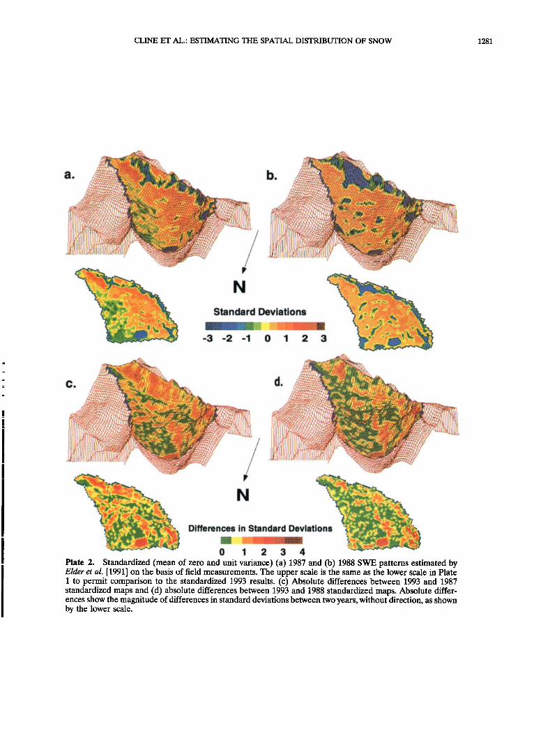
N Plate 1. Modeled distribution of SWEi and standardized (mean of zero and unit variance) SWEi for 1993 is shown in two projections. The upper projection illustrates the relationship of the modeled SWE patterns to topography, while the lower projection provides an undistorted view of the pattern locations. Two scales are shown with one color range: the upper scale shows the depth of SWE i in meters, while the lower scale shows standardized SWEi in units of standard deviations, to permit comparison to Figure 5.


' 3 -2 -1 0 I 2 3 ß

/:,, '•.:., ,• •- . ß .,•..,:.. "'e• ?'

N '"

, .

• . • - Differences in Standard Deviations *• ß . * -

0 I 2 3 4

Plate 2. Standardized (mean of zero and unit variance) (a) ]987 and (b) ]988 S• patterns estimated by Elder et al. []99]] on the basis of field measurements. The upper scale is the same as the lower scale in Plate ] to permit comparison to the standardized ]993 results. (c) Absolute differences be•een ]993 and ]987 standardized maps and (d) absolute differences be•een ]993 and ]988 standardized maps. Absolute differences show the magnitude of differences in standard deviations be•een •o years, without direction, as shown by the lower scale.


1200

8OO

40O

N!• ß Category 1 ß Category 2 ß Category 3

0 400 800

Measured Flux (W m -2)

1200

8OO

400

b)

ß v Category 5 ' 0 • ' I

1200 0 400 800 1200

Measured Flux (W m -2)

Figure 5. Scatterplots illustrating the overestimation of incident solar radiation during cloudy conditions (a) due to selected atmospheric parameters in TOPORAD. (b) During clear conditions the errors in modeled incident solar radiation are normally distributed with no apparent systematic bias.

the method of Marks and Dozier [1992], whereby nighttime snow surface temperatures are lower than air temperatures by 4-6øC and daytime snow surface temperatures lag behind air temperatures. However, since modeled air temperatures remained well above 0øC throughout most of the study period, snow surface temperatures were simply constrained to 0øC most of the time. We assumed a snow surface emissivity of 0.99 for computing surface longwave emissions using the Stefan- Boltzmann equation. To compute the turbulent fluxes, we assumed a roughness length of 0.002 m.

We modeled the turbulent fluxes using the bulk aerodynamic algorithms in SNTHERM.89.rev4 [Jordan, 1991], for two reasons: (1) Cline [1997] showed that they perform well under often extreme alpine conditions, and (2) a future improvement could be to fully integrate SNTHERM.89.rev4 into this modeling approach, eliminating the snow surface assumptions described above and providing physically modeled values for snow surface albedo, temperature, and emissivity.

2.3. Computing SWE i

A cumulative running total of the residual energy term A Qs + AQ•u of (1) was computed for each grid cell, providing a value for the total energy available for snowmelt (in MJ m -2) at each time step of the model run. For each remote sensing scene the total energy available for snowmelt was weighted by the area of the grid cell that was determined to have become snow-free since the previous remote sensing date, and converted to mass units to determine the amount of SWE that

would have initially existed on that portion of each grid cell that had become snow-free.

3. Results

We ran the model from midnight April 21 through midnight June 29, 1993. Three relatively cloud-free Landsat TM scenes with Emerald Lake coverage were available during or near this period: April 4, May 22, and June 22. A 16 day discrepancy between the first remote sensing date and the beginning of the meteorological data was resolved as follows. Temperature pro- files from three snow pits were used to assess the thermal status of the snowpack for initiating the model. Mean snowpack temperatures of 0øC and -0.1øC were measured in two snow pits excavated at 2817 m elevation near the inlet of

Emerald Lake on April 7. The mean snowpack temperature measured in a third pit excavated at higher elevation (2976 m) in the basin on April 10 was -3.9øC. From this information we estimated that by April 21 the snowpack would have warmed to 0øC everywhere throughout the basin, and snowmelt would have already occurred in the lower areas of the basin. A total discharge from the basin of 27,836 m -3 was recorded from April 4 through April 21. Considering that an unknown amount of this discharge was due to base flow, this quantity was on the order of 1% of the total basin discharge for the snowmelt season, which we considered to be negligible for purposes of an initial test of the modeling approach. This allowed us to ignore the energy exchanges during the first 16 days and also meant that we did not have to account for uncertain cold contents throughout the basin.

The minimum depth of SWEi modeled in the watershed was 0.08 m, and the maximum was 4.5 m. The modeled mean basin SWE/, (SWE), was 2.32 m. In general, the model estimates low SWE/on the steep ridge forming the southern watershed boundary, and on the steep arcuate cliff bands midway up the watershed (Plate 1). Larger magnitudes of SWEi are estimated for the flatter areas in the watershed, including most of the benches beneath the cliff bands.

Nineteen ninety-three was a heavy snow year, with several areas retaining snow into the 1994 water year. At the time of the last image, some fraction (ranging from 1% to 100% of the pixel area) of snow remained on 72.4% of the pixels in the basin, as determined from the fractional snow mapping. On these pixels the area-weighting scheme described in section 2.1 allowed SWEi to be fully determined for the fraction of the pixel that had become snow-free (where the snow cover depletion is defined), and a minimum estimate of SWE/to be determined for the remaining fraction based on the status of the cumulative energy balance. Thus, the modeled SWEi was effectively a minimum estimate for these pixels. We discuss the implications this has for the model results in section 4.2.

3.1. Evaluation of Distributed Incident Solar Radiation

With the exception of incident solar radiation the methods used to distribute the micrometeorological data across the basin conserved the measured data value at the pixel corresponding to the instrument station location. The measured incident solar radiation value was not conserved at the instru-


ment station pixel however, since the measurement was used only to derive an atmospheric parameter look-up table for TOPORAD, which in turn produced a modeled value for that pixel. We evaluated the performance of TOPORAD using the grouped Ts values (Table 1) by comparing the modeled values at the instrument station pixel to the measured incident solar radiation data. RMSE (root-mean-square errors) in the modeled fluxes ranged from 70 to 360 W m -2 for the different atmosphere categories. The overall RMSE for the three clear- est categories (3-5), representing 67% of the observations, was 127 W m -2, while the overall RMSE for the first two categories was much larger, at 335 W m -2. An obvious positive bias in the method (Figure 5) indicates that the selected atmospheric parameter sets failed to sufficiently reduce modeled incident solar radiation during cloudy periods. During clear periods, however, the modeled errors are normally distributed. While there is clearly room for improvement in this method, it is important to remember that with a large snow surface albedo, the net effect of these errors in the energy balance is reduced considerably.

4. Discussion

4.1. Evaluation of SWE i Results

We evaluated the results of the 1993 Emerald Lake test by (1) statistically comparing the mean and variance of the modeled SWE for the basin to independent data measured for a basin water balance study for 1993, (2) comparing the modeled spatial patterns of SWE to measured patterns from an earlier year, and (3) comparing the modeled total basin volume of SWE to results from a different SWE distribution model de-

veloped for the Emerald Lake watershed. Melack et al. [1996] determined a SWE of 2.19 m at peak

accumulation of the 1993 water year on the basis of 182 measurements from four snow courses within the basin. With es-

timated evaporation/sublimation and corrected precipitation data, this mean value provided satisfactory closure of the water balance with measured discharge from the basin in their study. The modeled SWE within the watershed boundaries was

2.32 m, a difference of 0.13 m, or 6%, from Melack et al.'s result. Considering their snow course data as one sample of SWE drawn empirically from the basin, we drew 10 random samples of N - 180 from the modeled SWE results and for each tested the null hypothesis that the measured and modeled samples came from the same parent population (/•mode•ed ---- /• ....... d; O•moOe•O -- O•m ...... •). We could not reject the null hypothesis for 9 of the 10 samples at the 2.5% significance level, and for 6 of 10 at the 5% significance level. Therefore the modeled results are not significantly different from the snow course data. Since the locations of the snow course measure-

ments are not precisely known, individual measurements may be correlated, and the comparison here is between a series of point measurements and samples of discrete areas (900 m 2 grid cells), we consider these statistical results cautiously and suggest only that SWE measurements obtained from traditional snow course methods support the model results.

Elder et al. [1991b] mapped SWE throughout Emerald Lake watershed for the 1986-1988 water years. Using a Bayesian classifier, they mapped zones within the watershed with similar physical properties and combined up to 354 field measurements of SWE with these zones using regression methods to map SWE patterns for each mapping date at 5 m resolution. They concluded that the mapping method produced realistic

representations of observed SWE patterns. With the assumption that SWE patterns in alpine basins are similar from year to year because of the strong influence of topography on snow accumulation, we compared the patterns mapped by Elder et al. [1991b] for peak accumulation of 1987 and 1988 to our modeled SWE pattern. We resampled their original data to 30 m resolution and standardized the results to zero mean and unit

variance to facilitate comparison (Plates 2a and 2b). In all three cases the lower tails of the SWE distribution (_•2 standard deviations below each year's SWE, including zero SWE) occurred along the steep southern ridge and on the steep arcuate cliff bands within the watershed, although the specific locations of low SWE values varied between cases. Subtraction

of the standardized 1987 and 1988 data from the standardized

1993 data indicated that overall the absolute differences were

low (Table 2), with 40% to 50% of the grid cells in each case being less than 0.5 standard deviations apart and with 70% to 80% of the grid cells being less than 1 standard deviation apart. The largest differences (_• 1.5 standard deviations) between the standardized SWE distributions were in the steep, low SWE areas (Plates 2c and 2d). In the 1987 case, slopes of 55 ø or greater were classified as snow-free; in the 1988 case snow-free areas were classified from field notes and oblique photos [Elder et al., 1991b]. In 1993 these steep areas had low modeled SWE, but no grid cells were estimated to be completely snow-free at peak accumulation. Thus the largest differences between the standardized 1987 and 1988 maps and the 1993 map can be attributed to the arbitrary treatment of snow-free areas in the 1987 and 1988 cases. Otherwise, the modeled SWE distributions are very similar.

Elder et al. [1995] presented a method of determining the SWE distribution in mountain basins using binary regression trees to classify field measurements of SWE into areas of similar accumulation based on physical (terrain) parameters and net solar radiation as independent variables. This method was also developed and tested in the Emerald Lake watershed and is considered to be superior to their previous attempts to distribute SWE over complex alpine terrain. Using the 1993 snow course data described above, this method yielded a total basin water volume at peak accumulation of 2,740,000 m 3 (2.34 m SWE) [Elder, 1995]. Our model provided a value of 2,741,990 m 3 (2.32 m SWE), a difference of less than 1%.

4.2. Discussion of Assumptions and Potential Errors

In this approach all of the error in modeled SWE lies in the determination of snow cover depletion and energy exchanges. Assuming that the subpixel snow cover classification methods used here are accurate, the error potential of snow cover depletion stems primarily from the registration accuracy between scenes. Determining fractional snow cover depletion in the above manner involves a classic change detection problem whereby an observed change in fractional snow cover within a given pixel from t n to tn•_ • could be the result of an actual change or could be due to misregistration of a given pixel between scenes. In the Emerald Lake test the three classified

scenes were each registered to the 30 m DEM simply by using 20 control points and a nearest-neighbor rectification algorithm. The small size of the study area in this case permitted an RMSE using this method of less than 0.25 pixels, but the potential for scene misregistration will increase as the model is applied over larger areas where there is greater inherent scene distortion. The determination of snow cover depletion will then need to be considered more carefully. To determine snow


Table 2. Frequency of Absolute Standard Deviation Differences Between Standardized 1993 and Standardized 1987 and 1988 SWE Maps

Standard Deviation Range

1993-1987 1993-1988

Number of Grid Cells Cumulative Frequency, % Number of Grid Cells Cumulative Frequency, %

0.0 -< •r < 0.5 558 39.0 759 53.1 0.5 -< •r < 1.0 432 69.3 360 78.3 1.0 -< •r < 1.5 271 88.2 182 91.0 1.5 -< •r < 2.0 98 95.1 72 96.1 2.0 -< •r < 2.5 59 99.2 46 99.3 2.5 -< •r < 3.0 9 99.9 9 99.9

•r >- 3.0 2 100.0 1 100.0

cover depletion at subpixel levels, we assumed that snow cover within a given pixel became smaller over time but otherwise did not change locations within the pixel. The validity of this assumption remains untested, and although it seems reasonable for the relatively small pixels used here, it may be inappropriate if larger p'rxels are used. A more critical problem is the potential for snow cover to increase over time. In the case presented here we had a simple situation of a consistent reduction in snow cover over time, which facilitated the determination of snow cover depletion. A situation where additional snowfall during the modeling period increases the snow cover would be more complicated, but to address it should require only a more involved tallying of the cumulative energy balance. Finally, it should be apparent that the frequency of scenes (temporal resolution) in the remote sensing time series effectively controls the precision to which SWE/can be determined.

We pointed out earlier that the duration of snow cover could not be completely determined in the study because of persis- tent snow cover through the final remote sensing date. Is the evidence we presented to support the validity of the model still meaningful if for many of the pixels SWE/represented a minimum value? Most of the remaining snow cover by June 22 was located at the foot of steep slopes and cliff bands, where deep snow accumulation typically occurs because of avalanching and wind redistribution [Elder et al., 1991b] (e.g., Figures 1 and 3). So we are effectively underestimating SWE/ in these deep snow areas. However, the 1993 snow course measurements included few of these areas, since safety considerations prevent many measurements from being made below steep slopes. We expect then that in both our statistical comparison to Melack's [1996] data and our comparison to Elder et al. [1995] modeled total basin water volume, we are comparing similarly underes- timated values for these areas, although the underestimation occurs for different reasons. Thus we contend that our com-

parison to field data is meaningful, but this problem illustrates the difficulty in validating snowmelt models in alpine basins.

In section 2 we pointed out 11 simplifying factors that were used in the extrapolation of micrometeorological data or in the energy flux computations: (1) spatially and temporally constant albedo assumed for TOPORAD's terrain reflection computation, (2) atmospheric parameters for TOPORAD simplified using five Ts classes, (3) simple daytime and nighttime lapse rates used for air temperature, (4) specific humidity assumed to be spatially constant at any given time step, (5) wind speed extrapolated using a simple elevation function, (6) incident longwave radiation modeled as a function of air temperature and relative humidity, (7) advective effects between and within pixels ignored, (8) snow surface albedo assumed to be spatially constant and to decrease only as a function of time, (9) snow

surface temperature computed using a simplistic model, (10) snow surface emissivity assumed to be spatially and temporally constant, and (11) snow surface roughness length assumed to be constant.

These are the major factors contributing to errors in the determination of energy exchanges. The satisfactory determination of SWE/ in this first test indicates that overall, these simplifying assumptions did not have a detrimental effect on our results. However, these factors may lead to large errors in individual components of the energy balance, which may tend to cancel within a single time step or over the duration of the model run. An example is the previously discussed overestimation of incident solar radiation during cloudy conditions. Such errors would result in a significant overestimation of SWE/ unless compensated by other factors. In our current work we are examining the validity of some of these assumptions and replacing others with more rigorous methods.

5. Conclusions

The modeling approach presented here produced an estimate of the magnitude and distribution of SWE in the test basin at peak accumulation that compared well to results from previous methods, snow course data, and to models of SWE distribution based on field measurements. The only data required were a time series of snow cover from remote sensing, a micrometeorological record during the snowmelt season, and a DEM. A rich data set was generated from the model, including spatially distributed snowmelt rates that are inherently coregistered to the computed SWE i distribution. The physical basis of the approach is advantageous as it reduces the need for parameter fitting or model calibration (none was performed here) and makes the model much more suitable for investigat- ing snowmelt response to changing boundary conditions. For example, to test hypotheses regarding snowmelt response to changing climate, this method could be used to back-calculate the distribution of SWE at peak accumulation in a given basin using actual measured micrometeorological data; then snowmelt could be recomputed using altered driving data reflecting the hypotheses to be tested. We believe this type of research application will be an especially useful application of this approach. There are opportunities for operational applications of this approach as well. Although the post facto determination of SWE distributions might appear to be too late for forecasting the timing, rate, and magnitude of snowmelt runoff, it is con- ceivable that similarities in SWE patterns within basins from year to year would make back-calculated SWE estimates for previous years useful for current forecasting. For example, SWE measurements from a few index sites within a basin might


be used to select a suitable historical SWEi distribution to represent the peak accumulation distribution for the current year. Remote sensing time series and energy balance modeling could then be used to refine the estimated SWE distribution as

the season progressed by reconciling the initial estimate with observed depletion rates and modeled snowmelt. Updating the current SWE distribution in this fashion, snowmelt forecasts could then be made using available meteorological forecasts.

Since widely applicable methods of determining SWE in mountain basins have never been available, this method should permit improved investigations of the influence of spatially distributed SWE and snowmelt on mountain hydrology. There is nothing in the approach restricting the size of the modeling domain, so it should be applicable to large regions. Because the model is physically based and needs little or no calibration, once SWEi is calculated for a given season the meteorological driving data can be safely modified to investigate hypotheses concerning hydrologic response to climate variability and change. Similarities in SWE patterns from year to year suggest that this modeling approach could potentially be used for water supply forecasting.

Acknowledgments. This research was supported in part by an In- terdisciplinary grant under NASA's Earth Observing System program and in part by grant EAR-9304933 from the National Science Foun- dation. We are especially grateful to W. Rosenthal, who classified the Landsat scenes. K. Elder, R. Harrington, W. Rosenthal, and M. Wil- liams provided helpful comments.

References

Anderson, E. A., Development and testing of snow pack energy balance equations, Water Resour. Res., 4(1), 19-37, 1968.

Bales, R. C., and R. F. Harrington, Recent progress in snow hydrology, U.S. Natl. Rep. Int. Union Geol. Geophys. 1991-1994, Rev. Geophys., 33, 1011-1020, 1995.

Baron, J. S., L. E. Band, S. W. Running, and D. Cline, The effects of snow distribution on the hydrologic simulation of a high elevation Rocky Mountain watershed using Regional HydroEcological Simu- lation System, RHESSys, Eos Trans. AGU, 74(43), 237, 1993.

Cline, D., Snow surface energy exchanges and snowmelt at a continen- tal, midlatitude alpine site, Water Resour. Res., 33(4), 689-701, 1997.

Dozier, J., A clear-sky spectral solar radiatiorl model for snow-covered mountainous terrain, Water Resour. Res., 16, 709-718, 1980.

Dozier, J., Spectral signature of alpine snow cover from the Landsat Thematic Mapper, Remote Sens. Environ., 28, 9-22, 1989.

Dozier, J., and J. Frew, Rapid calculation of terrain parameters for radiation modeling from digital elevation data, IEEE Trans. Geosci. Remote Sens., 28(5), 963-969, 1990.

Dozier, J., and D. Marks, Snow mapping and classification from Land- sat Thematic Mapper data, Ann. Glaciol., 9, 97-103, 1987.

Dubayah, R., Using LOWTRAN7 and field flux measurements in an atmospheric and topographic solar radiation model, in Proceedings of the International Geosciences and Remote Sensing Symposium (IGARSS) '91, 91CH2971-0, pp. 39-42, Inst. of Electr. and Electron. Eng., Piscataway, N.J., 1991.

Dubayah, R., J. Dozier, and F. W. Davis, Topographic distribution of clear-sky radiation over the Konza Prairie, Kansas, Water Resour. Res., 26(4), 679-690, 1990.

Elder, K., Snow distribution in alpine watersheds, Ph.D. dissertation, Univ. of Calif., Santa Barbara, 1995.

Elder, K., R. E. Davis, and R. C. Bales, Terrain classification of snow-covered watersheds, Proceedings of the 48th Eastern Snow Con- ference, pp. 39-49, 1991a.

Elder, K., J. Dozier, and J. Michaelson, Snow accumulation and distribution in an alpine watershed, Water Resour. Res., 27, 1541-1552, 1991b.

Elder, K., J. Michaelson, and J. Dozier, Small basin modeling of snow water equivalence using binary regression tree methods, in Biogeo- chemistry of Seasonally Snow-Covered Catchments, edited by K. A. Tonnessen et al., IAHS Publ. 228, 129-139, 1995.

Engman, E. T., and R. J. Gurney, Remote Sensing in Hydrology, Chap- man and Hall, New York, 1991.

Hungerford, R. D., R. R. Nemani, S. W. Running, and J. C. Coughlan, MT-CLIM: A mountain microclimate simulation model, Res. Pap. INT-414, Intermt. Res. Stn., U.S. Dep. of Agric., Ogden, Utah, 1989.

Idso, S. B., A set of equations for full spectrum and 8-14 /am and 10.5-12.5/am thermal radiation from cloudless skies, Water Resour. Res., 17, 295-304, 1981.

Jordan, R., A one-dimensional temperature model for a snow cover, Spec. Rep. 91-6, U.S. Army Cold Reg. Res. and Eng. Lab., Hanover, N.H., 1991.

Kneizys, F. X., E. P. Shettle, L. W. Abreu, J. H. Chetwynd, G. P. Anderson, W. O. Gallery, J. E. A. Selby, and S. A. Clough, User's guide to LOWTRAN7, Rep. AFGL-TR-88-0177, Air Force Geophys. Lab., Bedford, Mass., 1988.

Marks, D., and J. Dozier, Climate and energy exchange at the snow surface in the alpine region of the Sierra Nevada, 2, Snow cover energy balance, Water Resour. Res., 28(11), 3043-3054, 1992.

Martinec, J., and A. Rango, Areal distribution of snow water equiva- lent evaluated by snow cover monitoring, Water Resour. Res., 17(5), 1480-1488, 1981.

Melack, J. M., J. Sickman, A. Leydecker, and D. Marrett, Comparative analyses of high-altitude lakes and catchments in the Sierra Nevada: Susceptibility to acidification, final report, Cont. A032-188, Calif. Air Resour. Board, Sacramento, 1996.

Oke, T. R., Boundary Layer Climates, 2nd ed., Routledge, New York, 1987.

Rosenthal, W., and J. Dozier, Automated mapping of montane snow cover at subpixel resolution from the Landsat Thematic Mapper, Water Resour. Res., 32(1), 115-130, 1996.

Tarboton, D. G., M. J. Al-adhami, and D. S. Bowles, Preliminary comparisons of snowmelt models for erosion prediction, Proceedings of Western Snow Conference, 59, 79-90, 1991.

Tonnessen, K. A., The Emerald Lake watershed study: Introduction and site description, Water Resour. Res., 27, 1537-1539, 1991.

U.S. Army Corps of Engineers, Snow Hydrology, N. Pac. Div., Portland, Oreg., 1956.

Wolford, R. A., R. C. Bales, and S. Sorooshian, Development of a hydrochemical model for seasonally snow-covered alpine watersheds: Application to Emerald Lake watershed, Sierra Nevada, Cal- ifornia, Water Resour. Res., 32(4), 1061-1074, 1996.

R. C. Bales, Department of Hydrology and Water Resources, Uni- versity of Arizona, Tucson, AZ 85721. (e-mail: roger@hwr. arizona.edu).

D. W. Cline, National Operational Hydrologic Remote Sensing Center, Office of Hydrology, National Weather Service, 1735 Lake Dr. West, Chanhassen, MN 55317-8582. (e-mail: [email protected])

J. Dozier, Donald Bren School of Environmental Science and Man- agement, University of California, Santa Barbara, CA 93106. (e-mail: [email protected]).

(Received February 20, 1997; revised December 16, 1997; accepted December 23, 1997.)

estimating the spatial distribution of snow in mountain basins using remote sensing and energy

Documents