estimating the value of von kármán's constant in turbulent pipe flow

J. Fluid Mech. (2014), vol. 749, pp. 79–98. c© Cambridge University Press 2014doi:10.1017/jfm.2014.208

79

Estimating the value of von Kármán’s constantin turbulent pipe flow

S. C. C. Bailey1,†, M. Vallikivi2, M. Hultmark2 and A. J. Smits2,3

1Department of Mechanical Engineering, University of Kentucky, Lexington, KY 40506, USA2Department of Mechanical and Aerospace Engineering, Princeton University, Princeton, NJ 08544, USA

3Department of Mechanical and Aerospace Engineering, Monash University, VIC 3800, Australia

(Received 16 August 2013; revised 10 April 2014; accepted 12 April 2014;first published online 14 May 2014)

Five separate data sets on the mean velocity distributions in the Princeton University/ONR Superpipe are used to establish the best estimate for the value of vonKármán’s constant for the flow in a fully developed, hydraulically smooth pipe. Theprofiles were taken using Pitot tubes, conventional hot wires and nanoscale thermalanemometry probes. The value of the constant was found to vary significantly dueto measurement uncertainties in the mean velocity, friction velocity and the walldistance, and the number of data points included in the analysis. The best estimatefor the von Kármán constant in turbulent pipe flow is found to be 0.40 ± 0.02. Amore precise estimate will require improved instrumentation.

Key words: turbulent boundary layers, turbulent flows

1. Introduction

For wall-bounded flows over a smooth wall (assuming that the convection terms arenegligible), we can express the mean velocity variation in the so-called overlap regionin either inner scaling according to

U+ = 1κ

ln y+ + B, (1.1)

or in outer scaling as in

U+cl −U+ =−1κ

lnyR+ B∗. (1.2)

This result has classically been found through similarity hypotheses (von Kármán1930), mixing length concepts (Prandtl 1925), asymptotic matching (Millikan 1938),dimensional analysis (cf. Buschmann & Gad-el Hak 2007) or, more recently,high-Reynolds-number asymptotic analysis (George & Castillo 1997; Jiménez &Moser 2007). Here, U is the mean streamwise velocity, U+=U/uτ , y+= yuτ/ν, uτ =√τw/ν, τw is the wall stress, ρ is the fluid density and ν is the kinematic viscosity of

† Email address for correspondence: [email protected]

mailto:[email protected]

80 S. C. C. Bailey, M. Vallikivi, M. Hultmark and A. J. Smits

the fluid. Furthermore, U+cl =Ucl/uτ , where Ucl is the mean velocity on the centrelineand R is the radius of the pipe. Using (1.1) and (1.2), we can also write

U+cl =1κ

ln R+ + B+ B∗. (1.3)

The von Kármán constant κ and the additive constants B and B∗ were originallythought to be universal. Reviews of experimental data by Coles (Coles 1956; Coles& Hirst 1968) led to the values of κ = 0.40–0.41 being generally accepted, andthe values κ = 0.41, B = 5.2 and B∗ = 0.65 became commonly cited (Huffman &Bradshaw 1972; Bradshaw & Huang 1995; Schlichting & Gersten 2000). More recentexperiments, however, have suggested that these constants could depend on the flowunder consideration (Nagib & Chauhan 2008), or that the convection terms present inboundary layers act to alter the velocity profile compared to fully developed channeland pipe flows where they are strictly zero, appearing as a change in the constants(George 2007). For example, in turbulent boundary layers, Österlund et al. (2000)found κ = 0.384, B= 4.17 and B∗ = 3.6, while measurements in channel flows madeby Zanoun, Durst & Nagib (2003) indicated κ = 0.37 and B = 3.7. In pipe flow,McKeon et al. (2004a) found κ = 0.421, B = 5.60 and B∗ = 1.20, whereas Monty(2005) reported κ = 0.386 in a different pipe facility (and at lower Reynolds number).Zanoun et al. (2003) pointed out that values of κ from 0.33 to 0.43 and B from 3.5to 6.1 have been proposed, with no apparent convergence in time. A more recentreview, together with a historical perspective on logarithmic mean flow scaling andthe associated constants, is provided by Örlü, Fransson & Alfredsson (2010).

Many of these estimates of κ were based on regression fits to (1.1) or its derivative,which can easily lead to bias errors, especially when the lower and upper limits ofthe logarithmic region are still being debated (see e.g. Marusic et al. 2010; Smits,McKeon & Marusic 2011). To avoid such errors for pipe flow, additional meansfor obtaining κ were employed by Zagarola & Smits (1998) and McKeon et al.(2004a). One way, based on integrating (1.1) from the wall to the centreline andassuming complete similarity of the mean velocity profile, uses the Reynolds-numberdependence of the friction factor λ = 8(uτ/U)2, where U is the area-weighted bulkvelocity (for details, see Zagarola & Smits 1998). With ReD = 2UR/ν, the frictionlaw gives

1λ1/2= 1

2κ√

2 log elog(ReDλ

1/2)+C, (1.4)

where C is an empirical constant. Note that (1.3) and (1.4) are equivalent if U+cl andU+ differ by a constant. For pipe flow, this approach has the advantage that uτ canbe found with high precision by measuring the pressure drop along the pipe, and so(1.4) can give an alternative estimate of κ .

Despite these precautions, the pipe flow results of Zagarola & Smits (1998) andMcKeon et al. (2004a) have been disputed, including arguments that the Pitotprofiles required a turbulence correction (Perry, Hafez & Chong 2001; Nagib &Chauhan 2008). Such disputes could not be addressed without complementarythermal anemometry measurements made in the same facility, which have sincebeen obtained. Five complete data sets now exist on the mean velocity distributionin the Princeton University/ONR Superpipe at Reynolds numbers ranging across81× 103 6 ReD 6 1.8× 107. These profiles were taken using Pitot tubes, conventionalhot wires and nanoscale thermal anemometry probes (NSTAPs). Here, we aim to usethese data to establish the best estimate for the value of von Kármán’s constant forthe flow in a hydraulically smooth pipe, together with its uncertainty levels.

Estimating von Kármán’s constant in turbulent pipe flow 81

40

35

30

30

28

26

24

22

25

20

15

0.025

0.010

0.015

0.020

10

5

0100 101 102

103 104

103 104 105

104 105 106 107Re

D

FIGURE 1. (Colour online) Comparison of all mean velocity profiles included in thecurrent study: O, ZS; �, MLJMS; �, MMJS; ◦, VS; and 4, HVBS. Inset upper left:only data points falling in the range 1000< y+ < 0.1R+. Inset lower right: friction factordependence on ReD for all data sets.

2. Experimental data

The five data sets on the mean velocity in the Superpipe are the following: the Pitotdata of Zagarola & Smits (1998) (denoted ZS) and McKeon et al. (2004a) (denotedMLJMS); the conventional hot-wire data of Morrison et al. (2004) (denoted MMJS),whose mean flow results taken with hot-wire probes of sensing length of 500 and250 µm have not previously been published; the 60 µm sensing length nanoscalethermal anemometry probe (Bailey et al. 2010; Vallikivi & Smits 2014) results ofHultmark et al. (2012, 2013) (denoted HVBS); and a new Pitot data set Vallikivi(2014) acquired specifically for the present study (denoted VS). A comparison of meanvelocity profiles and ReD dependence of λ from all data sets is provided in figure 1.

The Superpipe is a closed-return facility, designed to produce high-Reynolds-numberpipe flow through pressurizing the working fluid, and it is described in detail byZagarola (1996) and Zagarola & Smits (1998). In all studies, the test pipe used wasthe same pipe used by Zagarola & Smits (1998), with R = 64.68 mm and relativeroughness of k/R = 2.3 × 10−6, being hydraulically smooth for R+ < 2.17 × 105

(ReD < 13.5 × 106) (McKeon 2003; McKeon et al. 2004a). Prior to the HVBSand VS experiments, the test pipe was disassembled to accommodate rough pipeexperiments, and then reassembled using optical inspection of every connection to


minimize mismatches between sections. The measurement station in all cases waslocated 392R downstream from the entrance to the pipe, to assure fully developed flow.The streamwise pressure gradient in the pipe was measured with 17 pressure taps overa distance of 50R to obtain the friction velocity, uτ . The particular flow conditionsfor each data set are given in the appropriate references, where further descriptions ofeach experiment may also be found. For the present analysis, to avoid any potentialbiasing by surface roughness effects, ZS and MLJMS data for R+ > 2.17 × 105

(ReD > 13.5 × 106) have been excluded. In addition, the ReD = 6 × 106 data fromMMJS and HVBS experienced relatively large temperature changes, resulting inanemometer drift, and so have also been excluded. Finally, the ReD = 5.5 × 104

case of MMJS was excluded due to errors identified in the probe calibration data(Hultmark, Bailey & Smits 2010). It was found that the measured R+ was found tobe within 3 % of 0.0655Re0.9125

D for the range of Reynolds numbers considered here.For the VS experiments, reported here for the first time, a Pitot tube with 0.40 mm

diameter was used and the static pressure was measured using two 0.40 mm staticpressure taps located in the pipe wall. This Pitot diameter was comparable to the0.89 mm and 0.30 mm diameter Pitot tubes used by Zagarola (1996) and McKeon(2003) respectively, and was equal to 0.006R or approximately 1000 viscous lengths atthe highest Reynolds number measured. The pressure difference was measured using aDatametrics 1400 transducer with a 2488 Pa range for all atmospheric pressure cases,and Validyne DP15 transducers with ranges 1379, 8618, 34 474 and 82 737 Pa for thepressurized cases, depending on the pressure. For the streamwise pressure gradientmeasurements, a 133 Pa MKS Baratron transducer was used for atmospheric casesand a 1333 Pa MKS transducer or Validyne DP15 34 474 Pa transducer was used forpressurized cases. All pressure transducers were calibrated prior to use. For calibratingthe lowest pressure range, a liquid manometer with uncertainty of less than ±0.40 %of the reading was used, whereas for the intermediate-range Validyne transducersan Ametek pneumatic dead-weight tester was used with accuracy of ±0.05 %. Thetunnel pressure was measured using Validyne DP15 transducers with 345, 3447 and27 579 kPa ranges, and these were calibrated using an Amthor dead-weight pressuregauge tester with accuracy of ±0.1 % of the reading.

Data were acquired at ReD ≈ 80 × 103, 150 × 103, 250 × 103, 500 × 103, 1 ×106, 2×106, 4×106, 6×106 and 10×106, with the Superpipe pressurized for ReD>150 × 103. The initial distance between the wall and the probe, y0, was determinedby using a depth measuring microscope (Titan Tool Supply Inc.). To position theprobe, a stepper motor traverse was used equipped with a linear optical encoder witha resolution of 0.5 µm (SENC50 Acu-Rite Inc.).

All Pitot data sets (ZS, MLJMS, VS) were processed using the static tap and shearcorrections proposed by McKeon & Smits (2002) and McKeon et al. (2003), withthe additional turbulence correction and associated near-wall correction discussedby Bailey et al. (2013). As done by McKeon et al. (2004a), we discard Pitot datafrom measurement points lying less than two probe heights from the surface. Toestimate the turbulence intensity required for applying the turbulence correction, thestreamwise turbulence intensity of HVBS is used for ReD 6 6× 106. For Pitot casesat higher Reynolds numbers, the turbulence intensity was estimated by assuming thatthe logarithmic scaling observed by HVBS was valid throughout the layer.

A comparison of the newly acquired VS Pitot data set to the HVBS NSTAP data settaken at the same Reynolds numbers is provided in figure 2. The results demonstratethe negligible difference between the two measurement techniques, after all applicablecorrections have been applied.


40

30

20

10101 102 103 104 105

Increasing ReD

FIGURE 2. (Colour online) Comparison of VS Pitot (◦) and HVBS (4) mean velocityprofiles at ReD = 80 × 103, 150 × 103, 250 × 103, 500 × 103, 1 × 106, 2 × 106 and4× 106. Note that successive Reynolds numbers are shifted vertically by 2uτ for clarity.

The fitting of (1.1), (1.3) and (1.4) to the data was conducted using the linearizedform of the equations applying a least-squares approach (implemented through theMATLAB function polyfit). The fit to (1.1) therefore returned κ−1 and B; to (1.3)it returned κ−1 and (B + B∗); and to (1.4) it returned (2

√2κ log e)−1 and C2. For

fitting to (1.3), U+cl was determined by a cubic fit to the three data points straddlingthe centreline, although there was a negligible difference when compared to the sameestimate using the measurement point located at the pipe centreline.

Estimates for the experimental uncertainties used in the uncertainty analysis arelisted in table 1. In most cases, given that much of the facility and instrumentationused was largely unchanged, these follow the values provided by ZS. Additionalsources of bias error are discussed in appendix A, and the approach used to estimatethe uncertainty in κ is described in appendix B.

3. The von Kármán constant as determined from the mean velocity profileWe first find κ using a least-squares fit of (1.1) to each individual velocity profile

within the range y+ > 1000 to y/R < 0.1. These values were selected to ensure thatthe fit was unambiguously contained within the range where a log law is expectedto hold, and our choice is not meant to suggest a particular range of validity of thelogarithmic scaling.

The results are presented in figure 3(a) and suggest a Reynolds-number-independentvalue of κ , but with large variations in experimental uncertainty across the Reynolds-number range and between measurements. Note that, with regards to uncertainty,there appears to be no advantage to using either thermal anemometry or Pitot tubemeasurement approaches, because the largest uncertainty is associated with thesmallest number of data points falling within the acceptance range and used for theregression fit. Thus, the uncertainty levels generally decrease with increasing ReD. Theexception is the early data set of ZS, where the higher uncertainty levels are mostlydue to the relatively large Pitot probe used by ZS, so that fewer measurement pointsfall within the fitting range. The most likely values for κ vary considerably amongthe data sets. For the earlier Pitot probe profiles, the ZS values lie between 0.39 and0.43, while the MLJMS data set suggests 0.40–0.42 (consistent with the previousestimate of 0.421 (McKeon et al. 2004a) at high Reynolds number). Both thermal


Dat

ase

tZ

SM

LJM

SM

MJS

HV

BS

VS

Sour

ceB

ias

Prec

.B

ias

Prec

.B

ias

Prec

.B

ias

Prec

.B

ias

Prec

.

Pito

tdi

ffer

entia

l(%

)±0.4

±0.8

a±0.4

±0.6

aN

/AN

/A±0.4

0.8

a

Pito

tco

rrec

tions

(%)

±1b

±0.3

c±1

b±0.3

cN

/AN

/A±1

b0.

3c

Hot

-wir

epr

ecis

ion

(%)

N/A

N/A

±0±0.4

a±0

±0.4

aN

/AH

ot-w

ire

calc

n.(%

)N

/AN

/A±1

±0±1

±0N

/AA

nem

omet

erdr

ift

(%)

N/A

N/A

±1±0

±1±0

N/A

ypo

sitio

n(µ

m)

118

541

541

55.

250.

513

.25

0.5

Tunn

elpr

essu

re(%

)±0.3

±0.3

±0.3

±0.3

±0.3

Pres

sure

grad

ient

(%)

±(0.

17–0.8

3)±(

0.17

–0.8

3)±(

0.17

–0.6

8)±(

0.17

–0.6

8)±(

0.17

–0.6

8)Te

mpe

ratu

re(%

)±0.0

5±0.0

5±0.0

5±0.0

5±0.0

5D

ynam

icvi

scos

ity(%

)±0.8

±0.8

±0.8

±0.8

±0.8

Pipe

radi

us(%

)±0.0

6±0

±0.0

6±0

±0.0

6±0

±0.0

6±0

±0.0

6±0

TAB

LE

1.B

ias

and

prec

isio

nun

cert

aint

yes

timat

es.

Whe

rea

sing

leva

lue

isst

ated

acro

ssbo

thbi

asan

dpr

ecis

ion

colu

mns

,th

esa

me

valu

ew

asus

edfo

rbo

thbi

asan

dpr

ecis

ion

unce

rtai

nty.

(a)

Val

uees

timat

edfr

omda

tasc

atte

r.(b

)V

alue

estim

ated

base

don

resu

ltsof

Bai

ley

etal

.(2

013)

.(c

)V

alue

estim

ated

from

scat

ter

inm

easu

red

velo

city

grad

ient

.


0.45

103 104 105

105 106 107

0.450.35

R+

103 104 105

R+103 104 105

R+

103 104 105

R+

ReD

105 106 107ReD 105 106 107Re

D

105 106 107ReD

0.40

0.450.35

0.40

0.450.35

0.40

0.45

0.40

0.35

0.35

0.40

0.45

0.450.35

0.450.35

0.450.35

0.450.35

0.35

0.40

0.40

0.40

0.40

0.40

ZS

MLJMS

MMJS

HVBS

ZS

MLJMS

MMJS

HVBS

VS VS

(a) (b)

FIGURE 3. (Colour online) Value of κ as estimated from least-squares fit of (1.1) to themean velocity profiles measured at different Reynolds numbers for the range of data pointslying in the range (a) 1000< y+< 0.1R+ and (b) 3(R+)1/2 < y+< 0.15R+. Dot-dot-dashedlines indicate 95 % confidence limits, and dashed lines indicate 50 % confidence limits.Horizontal black dotted lines indicate the values of κ = 0.40 and κ = 0.421.

anemometry cases give estimates of κ varying between 0.38 and 0.40, whereas themost recent Pitot data set indicates a value between 0.40 and 0.41.

In addition to the conservative range (y+ > 1000 to y/R< 0.1), we also consideredthe overlap layer range of 3(R+)0.5 < y+ < 0.15R+ used by Marusic et al. (2013)based on the estimate by Klewicki, Fife & Wei (2009) of the range y+ > 2.6(R+)0.5where viscous force loses leading-order influence. The resulting estimate of κ wasfound to be Reynolds-number-dependent for ReD . 2× 106, as shown in figure 3(b).Note that y+ = 3(R+)0.5 ≈ 600 at ReD ≈ 2 × 106, corresponding to the lower limitobserved by McKeon et al. (2004a). Above this Reynolds number, the values of κestimated become very close for the two different limits. Virtually identical resultswere observed when the upper limit was reduced to y/R = 0.1, suggesting that theReynolds-number dependence is caused by the R+ dependence of the lower limit.Therefore, the current results do not support the Reynolds-number-dependent lowerlimits used by Marusic et al. (2013).

4. The von Kármán constant as determined from Reynolds-number dependenceof bulk propertiesAlthough regression fits to the mean velocity profiles can provide an estimate of κ ,

the procedure is sensitive to the range of y+ values selected for fitting, and to small


0.45

103 104 105

105 106 107

0.450.35

R+

103 104 105

R+

103 104 105

R+

103 104 105

R+

ReD

105 106 107ReD

105 106 107ReD

105 106 107ReD

0.40

0.450.35

0.40

0.450.35

0.40

0.45

0.40

0.35

0.35

0.40

0.45

0.450.35

0.450.35

0.450.35

0.450.35

0.35

0.40

0.40

0.40

0.40

0.40

ZS

MLJMS

MMJS

HVBS

ZS

MLJMS

MMJS

HVBS

VS VS

(a) (b)

FIGURE 4. (Colour online) Value of κ estimated from least-squares fit of (a) equation(1.4) (friction factor fit) and (b) equation (1.3) (centreline velocity fit) shown as a functionof the lowest Reynolds-number case used for the regression fit. Dot-dot-dashed linesindicate 95 % confidence limits, and dashed lines indicate 50 % confidence limits.

errors in uτ (see e.g. Örlü et al. 2010). However, for pipe flow a valid estimate of κmust satisfy (1.1), (1.2), (1.3) and (1.4). Therefore, given a sufficient Reynolds-numberrange, one can also estimate κ from the Reynolds-number dependence of the bulk flowproperties. This was the approach taken by Zagarola & Smits (1998) and McKeonet al. (2004a).

Figure 4 shows the value of κ estimated by fitting (1.4) and (1.3) to the centrelinevelocity data and the friction factor data, respectively. The results are shown as afunction of the lowest Reynolds number included in the fit. For example, for thehighest Reynolds number shown, κ was estimated from fitting only the two highestReynolds-number cases; each successively lower Reynolds-number data point on thefigure represents the results from a curve fit with one additional point included in thefit. Hence the lowest Reynolds number plotted represents the estimate of κ determinedfrom fitting the entire data set.

As noted by McKeon et al. (2004a) with respect to the MLJMS data set, we seethat for ReD > 300 × 103 the estimates for all data sets become Reynolds-number-independent, except for the highest Reynolds-number values, where the number ofpoints in the fit is reduced and the uncertainty increases significantly. For ReD> 300×103, fitting (1.4) or (1.3) gives similar values, although the latter estimate is subjectto slightly higher uncertainty because it relies on a single measurement of U+cl at each


0.46

0.44

0.42

0.40

0.38

0.360.460.440.420.400.380.36

ZS

MLJMS

MMJS

HVBS

VSZ

S

ML

JMS

MM

JS

HV

BS

VS

Prob

abili

ty d

ensi

ty

(a) (b)

FIGURE 5. (Colour online) (a) Values of κ estimated from each data set with error barsindicating 95 % confidence interval. For each data set, the value on the left is obtainedfrom the regression fit to (1.1); the one in the centre is from the regression fit to (1.3); andthe one on the right is from the regression fit to (1.4). (b) Probability density functionsof κ for each data set found by combining the uncertainty of all three estimates.

Reynolds number. The ZS, MLJMS and MMJS data sets return a value of κ ≈ 0.42consistent with the McKeon et al. (2004a) estimate of κ = 0.421. However, the morerecent HVBS and VS data indicate κ≈0.41 and 0.40, respectively. In addition, we seethat the uncertainties in the thermal anemometry data sets are much higher than that ofthe Pitot data sets, primarily because the thermal anemometry data cover a smaller andlower Reynolds-number range. A fit of (1.4) was also applied to the high-Reynolds-number friction factor data of Swanson et al. (2002) (tabulated in McKeon et al.2004b). The resulting estimate of κ was found to depend strongly on the Reynolds-number range selected for the fit, varying between 0.41 and 0.5.

5. DiscussionThe different estimates of κ from each data set are summarized in figure 5. For

the regression fit to (1.1), we use the value determined from the highest Reynolds-number case, where the uncertainty is lowest due to the number of data points in thelogarithmic region. For the estimates determined from regression fits to (1.3) and (1.4),we use the value determined from fitting to ReD> 3× 105, which comprises the rangewhere the estimate becomes ReD-independent and the uncertainties are lowest due tothe number of data points included in the fit.

If we assume that the log law is valid, then (1.1), (1.3) and (1.4) must besimultaneously valid, and inspection of figure 5(a) reveals two important points.First, no single value of κ is within the 95 % uncertainty bounds of all five datasets. This indicates that one or more sources of uncertainty remain undetected whilealso reflecting the difficulty inherent in determining κ experimentally. Second, theestimates obtained by fitting equations (1.3) and (1.4) are consistently higher thanthose obtained by fitting (1.1), suggesting that these undetected errors are consistentlybiasing the estimate.

Many factors contribute to the overall uncertainty, but the primary ones are theestimate of y0, the method chosen to integrate the mean velocity profile near the wallin order to find U, drift in the thermal anemometry measurements, and turbulence


corrections to the Pitot probe data (see appendix A). For example, the turbulencecorrection influences the value of κ obtained by fitting (1.1) by 2 %, and a relativelysmall (0.08 % of R) uncertainty in the wall distance can change κ by up to 3 %,whereas estimates obtained by fitting equations (1.3) and (1.4) are nearly unaffected bythese factors. On the other hand, the estimates obtained using (1.3) and (1.4) are verysensitive to the different pressure transducers used to obtain the velocity and pressuregradient, as well as the integration methods for estimating bulk properties. Estimatesobtained from the hot-wire data are extremely sensitive to any type of drift, whereestimates obtained using (1.3) and (1.4) can be influenced by up to 6 % even withhigh-quality calibrations with less than 1 % drift. Overall, it can be seen that there isno measurement technique or method of analysis that could be identified as the mostprecise.

Although the 95 % confidence intervals indicate that no value of κ is supported byall data sets, within each data set there exists a range of possible values, following theassumption that (1.1), (1.3) and (1.4) must be simultaneously valid. Thus ZS indicates0.41< κ < 0.42; MLJMS indicates 0.41< κ < 0.43; MMJS indicates 0.39< κ < 0.41;HVBS indicates 0.39 < κ < 0.41; and VS indicates 0.39 < κ < 0.41. However, sincethese ranges represent an overlap of three separate 95 % confidence ranges, theconfidence of κ lying within this range for each data set is actually lower. Thisis demonstrated by the probability density functions (p.d.f.s) shown in figure 5(b),which were compiled from combining all three methods used to estimate κ using theuncertainty analysis described in appendix B. We see that the most probable value ofκ is 0.40 for the three most recent data sets, arising from reduced uncertainty in thefitting of (1.1) at high Reynolds numbers combined with the higher uncertainty infitting equations (1.3) and (1.4) for these data sets. Conversely, the ZS and MLJMSdata sets indicate the most probable value of κ is 0.42 due to the agreement betweenthe fits of (1.3) and (1.4) (and reduced uncertainty) for these data sets.

Using these p.d.f.s, it can also be determined that the confidence of κ being withinthe intervals of overlap in 95 % confidence for the three techniques is approximately50 % or less for the ZS, MLJMS, MMJS and HVBS data sets (i.e. a 50 % chance that0.41< κ < 0.42, 0.41< κ < 0.43, 0.39< κ < 0.41 and 0.39< κ < 0.41, respectively).In comparison the agreement between the three estimates of κ for the VS data setresults in a 73 % confidence that 0.394<κ < 0.408, indicating that this data set is theone least affected by undetected bias errors.

As previously noted, this disagreement between the multiple estimates of κ cannotbe accounted for using the known bias and precision errors provided in table 1,suggesting the presence of undetected bias errors. For obvious reasons, it is notpossible to identify the source of these undetected errors. However, examining alldata sets as a whole does reveal symptoms of these errors, which provide furtherinformation that can be used to assess the data. We start first by noting that (1.4)can be rewritten as

U+ = 1κ

ln R+ + B+ B∗ + E, (5.1)

where E = U+cl − U+, which includes contributions from the difference between theactual velocity profile and (1.1) extrapolated to the wall and to the core region. Asnoted by Zagarola & Smits (1998), the difference between the true velocity profile and(1.1) near the wall is Reynolds-number-dependent but, for a fixed lower limit of theoverlap layer, should vanish when R+ is large. Hence, assuming no Reynolds-numberdependence in the wake contribution to U+ and constant B∗, at sufficiently high R+,E should also be constant. We examine this Reynolds-number dependence in figure 6.


4.8

4.6

4.4

4.2104 105

104103 105

106 107

ReD

FIGURE 6. (Colour online) Reynolds number dependence of E = U+cl − U+: O, ZS; �,MLJMS; �, MMJS; ◦, VS; and 4, HVBS.

All data sets demonstrate Reynolds-number dependence in E for ReD < 300× 103,consistent with the Reynolds-number dependence previously observed when estimatingκ from bulk flow properties. For ReD > 300× 103 the ZS and HVBS data sets appearReynolds-number-independent whereas the MLJMS and VS data set exhibit ReDdependence for ReD > 3 × 106. This Reynolds-number dependence at high Reynoldsnumbers could be due to a Reynolds-number-dependent experimental bias impacting E,as would appear, for example, through the integration of U with insufficient resolutionnear the wall as discussed in § A.3. However, given the agreement with the VS Pitotand NSTAP, and that the Reynolds-number dependence is not evident on the ZSdata set, which was acquired with an even larger Pitot tube, we cannot conclusivelyattribute the Reynolds-number dependence exclusively to the use of Pitot probesand thus also cannot discount the possibility that the observed Reynolds-numberdependence could be due to a real phenomenon, such as a ReD-dependent inner limitof the overlap region.

Also clearly evident in figure 6 is a shift in E for the MLJMS and MMJS data setswith respect to the other four data sets. These two data sets are also the ones with thegreatest disparity between κ estimated from (1.3) and (1.4). The source of this shift inE becomes apparent when closely examining the Reynolds-number dependence of U+

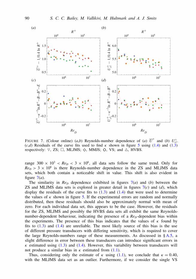
and U+cl , as done in figure 7(a,b). In these figures, 1/0.4 ln R+ has been subtractedfrom the values to de-trend the Reynolds-number dependence in a way that wouldresult in a constant value if κ = 0.4. It is clear by comparison of figures 7(a) and (b)that the shift in E for the MLJMS and MMJS data sets arises from a bias introducedinto the estimate of U. It is not possible to identify where this bias enters into theestimate, although the Reynolds-number independence of this bias suggests that it isnot due to error in y0.

The bias observed in the MLJMS and MMJS area-averaged data suggests thatthe κ estimated via (1.3) is a more reliable estimate. However, close examinationof figure 7(b) shows some interesting behaviour. As noted previously, when plottedin this way, a constant value of U+cl − 1/0.4 ln R+ would occur if κ = 0.4. Asexpected from the previous discussion, this is only the case over the entire rangeReD > 300 × 103 for the VS (and possibly the HVBS) results. However, within the


104 105

106 107

ReD

ReD

1.5

1.0

0.5

104 105

106 107

6.0

5.5

5.0

106 107

0.2

0

–0.2

106 107

0.2

0

–0.2

(a) (b)

(c) (d)

FIGURE 7. (Colour online) (a,b) Reynolds-number dependence of (a) U+ and (b) U+cl .(c,d) Residuals of the curve fits used to find κ shown in figure 5 using (1.4) and (1.3)respectively: O, ZS; �, MLJMS; �, MMJS; ◦, VS; and 4, HVBS.

range 300 × 103 < ReD < 3 × 106, all data sets follow the same trend. Only forReD > 3 × 106 is there Reynolds-number dependence in the ZS and MLJMS datasets, which both contain a noticeable shift in value. This shift is also evident infigure 7(a).

The similarity in ReD dependence exhibited in figures 7(a) and (b) between theZS and MLJMS data sets is explored in greater detail in figures 7(c) and (d), whichdisplay the residuals of the curve fits to (1.3) and (1.4) that were used to determinethe values of κ shown in figure 5. If the experimental errors are random and normallydistributed, then these residuals should also be approximately normal with mean ofzero. For each individual data set, this appears to be the case. However, the residualsfor the ZS, MLJMS and possibly the HVBS data sets all exhibit the same Reynolds-number-dependent behaviour, indicating the presence of a ReD-dependent bias withinthe experiments. The presence of this bias indicates that the values of κ found byfits to (1.3) and (1.4) are unreliable. The most likely source of this bias is the useof different pressure transducers with differing sensitivity, which is required to coverthe large Reynolds-numbers range of these measurements. As discussed in § A.5, aslight difference in error between these transducers can introduce significant errors inκ estimated using (1.3) and (1.4). However, this variability between transducers willnot produce a similar bias in κ estimated from (1.1).

Thus, considering only the estimate of κ using (1.1), we conclude that κ = 0.40,with the MLJMS data set as an outlier. Furthermore, if we consider the single VS


4.0

3.5

3.0

2.5

5.0

4.5

4.0

6.0

5.5

5.0

103 104

(a)

(b)

(c)

FIGURE 8. (Colour online) Plots of U+ − κ−1 ln y+ within the range 1000< y+ < 0.1R+for (a) κ = 0.38, (b) κ = 0.40 and (c) κ = 0.42: O, ZS; �, MLJMS; �, MMJS; ◦, VS;and 4, HVBS. Highlighted profiles are the highest Reynolds-number profiles for each dataset.

data set, we could therefore conclude that κ = 0.40± 0.01. However, doing so wouldnecessarily assume that only this data set was free of undetected bias errors, whichaffected all previous data sets. Such filtering of data sets, although not completelyarbitrary, is not prudent, and therefore we must consider the complete collection ofdata. The lack of consensus suggests that the actual uncertainty in κ is likely to behigher than that given by any single data set, and a more conservative estimate isκ = 0.40 ± 0.02. The profiles in the range 1000 < y+ < 0.1R+ are compared to thisrange of κ in figure 8, in which the logarithmic region should appear constant andequal to B over the entire overlap layer. The results for κ= 0.40 in figure 8(b) suggesta value of B= 4.5± 0.3 when κ = 0.40.

An apparent Reynolds-number-dependent trend in B can also be discerned infigure 8(b), reminiscent of the expected behaviour caused by the onset of roughnesseffects. However, as demonstrated in figure 9(a), which shows the value of Bdetermined by fixing κ = 0.40, this trend is also the same as that observed infigures 7(a) and (b) and already attributed to bias error. The similarity of the trendsin figures 8 and 7(b) is not unexpected given the interrelationship between (1.1) and(1.3), and the trend in figure 8(b) is thus a manifestation of the same bias error. Thisis further confirmed in figure 9(b), which shows no obvious trend in the value of Bproduced by the same regression fit to (1.1) that produced the values of κ shown infigure 3(a).

Our estimate of κ = 0.40 is identical to the recent values found for channel flow byJiménez & Moser (2007) and Schultz & Flack (2013), and the uncertainty limits areconsistent with the currently accepted values for boundary layers of κ = 0.38–0.39


104 105 104 105

106 107

ReD

106 107

ReD

(a) (b)

5.0

4.8

6

5

4

4.6

4.4

4.2

4.0

FIGURE 9. (Colour online) Plots of additive constant B determined (a) when κ is fixedat 0.40 and (b) from least-squares fit to (1.1):O, ZS; �, MLJMS; �, MMJS; ◦, VS; and4, HVBS.

(Österlund et al. 2000; Nagib & Chauhan 2008; Marusic et al. 2013). It wouldappear, therefore, that the present results support the existence of a universal value ofκ . However, inspection of figures 8(a) and (c), which show U+−κ−1 ln y+ for κ=0.38and 0.42, provides little support for the proposed boundary layer value of κ = 0.38within the current pipe flow results. It should also be noted that the present resultsalso required a large range of Reynolds number and the use of the most conservativeestimate of the logarithmic region to date to obtain a Reynolds-number-independentestimate of κ . To obtain a comparable estimate for turbulent boundary layers andchannels would require significantly more data with a Kármán number >10 000 thanis currently available (at least for data accompanied by an independent skin frictionmeasurement).

6. ConclusionsFor the first time, all available smooth-wall mean flow data sets acquired in the

Princeton University/ONR Superpipe were analysed to determine the von Kármánconstant, κ , using three different methods. Owing to its large Reynolds-number rangeand controlled conditions, this facility offers a unique opportunity to estimate thevalue of κ and its attendant uncertainty.

Unlike most prior studies investigating the value of κ for pipe flow, we do notlimit our analysis to a single data set. We find no clear consensus on the value of κobtained from multiple data sets measured largely independently in the same facility,even following the application of all known corrections and taking into account allthe known uncertainties. This suggests that the actual uncertainty in κ is likely to behigher than that given for any single data set studied. Based on all our observations,we therefore estimate the value of κ for high-Reynolds-number pipe flow to be0.40± 0.02. The fact that, even with this facility, using modern instrumentation, thevalue of κ can only be determined to within this precision is a notable result. Inorder to obtain a more precise estimate of κ , improved experimental techniques arerequired, accompanied by carefully conducted experiments and analysis. It should alsobe noted that evaluation of κ in turbulent boundary layers is even more challenging,given that measurements of uτ are less accurate. Contrary to what has been suggestedin previous work, we found that differences between values of κ cannot be attributedonly to the differences between hot-wire anemometry and Pitot tube measurements.


Acknowledgements

This work was supported through ONR grant N00014–09-1-0263 (Program ManagerRonald Joslin). The authors would also like to thank all reviewers for their helpfulcomments, in particular Referee 4, who suggested looking at the Reynolds-numberdependence of the difference between (1.3) and (1.4).

Appendix A. Bias error effects on determination of von Kármán constant

Uncertainties may be divided into bias errors and precision errors. Here, we treatprecision uncertainty as the expected variation that would occur amongst repeatedmeasurements of the same quantity as reflected through experimental scatter. Biaserror is more difficult to identify and we treat it as a consistent deviation betweenthe measured and true quantities as introduced by the experiment set-up, procedureor analysis. The estimated errors for the data sets under consideration are provided intable 1, where uncertainty values derived from stated manufacturer values are treatedas bias error. Here we discuss several additional sources of bias error that can play arole in estimates of κ , and investigate the impact of each source on the estimate.

A.1. Impact of Pitot probe correctionsPitot probe corrections for shear, near-wall, viscous and finite static tap size arediscussed in great detail in many sources (see e.g. Tavoularis 2005; Tropea, Yarin& Foss 2007). With the exception of eliminating data points less than two probediameters from the surface, the complete correction suite used here is described inBailey et al. (2013) and has been demonstrated to result in Pitot measured meanvelocity agreeing with that measured by hot wires to within 1 %. This differencetherefore can be used as an approximation of the bias error that can be expectedin the measured mean velocity. However, the source of this bias should not beconsidered exclusive to the Pitot and the accuracy of its corrections, but can equallybe attributed to uncertainty in the hot-wire mean velocity.

Of particular interest for the Pitot measurements is the magnitude of the correctionfor turbulence effects, which has previously been observed to significantly bias theestimate of κ found using mean flow profiles (Perry et al. 2001; Nagib & Chauhan2008). To assess the effect of this correction on estimates of κ , we repeated theanalysis without the turbulence correction. The effect of not using the turbulencecorrection was found to be an increase in estimated κ of +2 % when determinedusing (1.1) and bias of −0.2 % and +0.2 % when using (1.3) and (1.4) respectively.

A.2. Initial probe position

The effects of initial probe position are discussed in detail in Örlü et al. (2010),which illustrates how accurate determination of wall position is necessary to correctlydeduce mean and turbulence quantities. In the Superpipe, the wall layer thickness is64.68 mm and, at ReD = 1.3× 107, the viscous length is only 300 nm. Therefore, aninaccurate estimate of wall position can have significant effect on the mean velocityprofile. To minimize this zero position error, the ZS data set used a capacitance-basedmethod to determine the zero position to within 40 µm, and the MLJMS data setused electrical contact between the probe and surface to identify initial probe positionand cite accuracies of 5 µm. For the MMJS data, no details were available regardinghow the initial probe distance was determined. For the HVBS and VS data, initial


probe position was determined via depth measuring microscope, with the zero locationmarked using an electrical contact, and a 5 µm uncertainty is estimated. Note thatthese cited values are likely to be underestimates of the true bias, which can arisefrom error in estimating Pitot probe diameter, probe orientation with respect to thewall, hot-wire probe distortion and rotation relative to the wall plane, the methodused to measure wall distance, or the possibility that electrical contact is rarely madeat a clearly defined and repeatable point (Hutchins & Choi 2002). These errors arealso further compounded in the Superpipe facility due to lack of optical access to themeasurement station and therefore inability to verify the relative position of the probeto the wall.

To illustrate how uncertainty can propagate into the estimate of κ , we artificiallybiased the zero position of the VS data set by +50 µm (12.5 % of the probe diameter,corresponding to a bias of approximately 1.5 viscous units at the lowest Reynoldsnumber and 125 viscous units at the highest Reynolds number). For κ estimatedfrom (1.1), there was a resulting bias in κ of −1 % at ReD = 1 × 106 to −3 % atReD > 4 × 106, corresponding to biasing of κ estimates from −0.004 to −0.01. Asmight be expected, the effect on the estimates of κ using (1.4) and (1.3) were muchless dramatic, corresponding to Reynolds-number-dependent bias in κ estimate from−0.01 % to −0.05 % using (1.4) and +0.005 % to +0.05 % using (1.3).

A.3. Estimate of area-averaged flow velocity from discrete dataAn associated error to that of initial probe position, which could have a noticeableeffect on the estimate of κ using (1.4), is the numerical integration scheme used todetermine area-averaged velocity to calculate the Reynolds number. As the Reynoldsnumber increases, and the inner layer thins accordingly, there is a potential Reynolds-number-dependent bias introduced into any estimate of area-averaged velocity due toan inability to resolve this high-shear region. This compounds any error introducedby the order of the numerical integration scheme used. In this study, we have usedsecond-order-accurate trapezoidal integration and, where necessary, have extrapolatedthe profile down to the wall with data measured at lower Reynolds numbers andassuming wall scaling is valid. Not performing this extrapolation process was found tohave a surprisingly significant effect on κ determined using (1.4), with a bias in κ oftypically +3 %, +0.4 %, +1 % and +1 % being observed by neglecting this step forthe ZS, MLJMS, MMJS and VS data sets respectively. For the HVBS data set, theclosest measurement point was always within the buffer layer and the extrapolationprocess was not required.

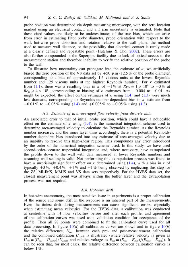
A.4. Hot-wire driftIn hot-wire anemometry, the most sensitive issue in experiments is a proper calibrationof the sensor and some drift in the response is an inherent part of the measurements.Even the tiniest drift during measurements can cause significant errors, especiallywhen estimating mean velocities. For the HVBS data, a calibration was conductedat centreline with 14 flow velocities before and after each profile, and agreementof the calibration curves was used as a validation condition for acceptance of theprofile. Then all 28 points were combined to fit the calibration curve used for alldata processing. In figure 10(a) all calibration curves are shown and in figure 10(b)the relative difference, Urel, between each pre- and post-measurement calibrationand the combined calibration Ucomb is illustrated (where relative velocity is given asUrel= (Ucal−Ucomb)/Ucomb and relative voltage as Erel= (Ecal−Emin)/(Emax−Emin)). Itcan be seen that, for most cases, the relative difference between calibration curves isbelow 1 %.


Voltage E (V)

Vel

ocity

U (

m s

–1)

Erel

15

10

5

0.6 0.8 1.0 1.2 1.40

0.05

0.04

0.03

0.02

0.01

0

–0.05

–0.04

–0.03

–0.02

–0.01

Ure

l

0.60.40.20 0.8 1.0

FIGURE 10. (Colour online) Calibration points and curves for all cases in the HVBSdata set. Dashed line and circles indicate pre-calibration fit; dotted line and squarespost-calibration fit. (a) Calibration points and corresponding fitted curves. (b) Relativedifference Urel of the calibrations compared to the combined calibration fit.

To estimate the error from this minimal drift, all data were processed usingpre- and post-measurement calibrations separately and values of κ were comparedto the values found using combined calibration curves. Despite the agreementapparent in figure 10, regression fit to (1.1) showed differences in κ of up to 1.1 %,whereas fits to (1.3) and (1.4) had variations up to 6.3 % and 5.5 % respectively.Additionally, an interpolation scheme was also attempted to transition between pre-and post-measurement calibration curves over the course of the profile measurements.When this was employed, the estimate of κ from regression fit was found to vary upto 0.6 % and that to (1.3) and (1.4) varied 4.6 % and 4.6 % respectively. Therefore itcan be seen that even a slight variation in probe response over the course of a profilemeasurement will significantly impact the estimate of κ and thus mean velocitymeasurements with hot wires must be treated with caution.

A.5. Use of multiple transducers over a large Reynolds-numbers rangeThe advantage of the Superpipe is not strictly the high Reynolds numbers it canachieve, but also its achievable Reynolds-number range. It is this range, achievedby pressurizing the working fluid, that makes the use of (1.3) and (1.4) feasible forobtaining estimates of κ . It is also the insensitivity of (1.3) and (1.4) to the biaserrors discussed in §§A.1–A.3 that makes them attractive for estimating κ . However,measuring the quantities in (1.3) and (1.4) accurately over the range of Superpipeoperating pressures requires the use of multiple pressure transducers of varyingsensitivity, each of which requires individual calibration. Therefore, the final sourceof bias error that will be described here is the error associated with using multipletransducers to measure the quantities used in (1.3) and (1.4). This error will arisefrom even slight differences in the calibrations between the different transducers.

To illustrate the impact that this error could have on the estimate of κ , were-analysed the MV data set after artificially adding a −1 % error in the Pitottransducer for 2.5× 105 6 ReD 6 1× 106 and 1 % error for ReD > 6× 106. Whereas


κ determined by (1.1) changed by 0.5 % and −0.5 % respectively in the affectedReynolds-number ranges, κ determined from (1.3) and (1.4) were found to change by−1.5 % to −8 %, depending on the Reynolds-number range used for the fit. A similaranalysis conducted with the bias applied to the pressure gradient transducer resultedin a 1–8 % change in κ using (1.3) and (1.4) and −0.5 % and +0.5 % using (1.1).Estimates of κ were found to be much less sensitive to bias errors in the transducerused to measure the Superpipe operating pressure, with a negligible effect on estimatesusing (1.1) and only a 0.1–0.5 % bias resulting when using (1.3) and (1.4).

Appendix B. Overview of uncertainty estimation processOne of the primary goals of this study was to provide a detailed estimate of the

accuracy to which we can experimentally determine κ . To do this, we employed aMonte Carlo-based error analysis, so that variables such as integration scheme andnumber of data points used in the regression fits would also be factored into the finaluncertainty estimate. Here we describe the approach used.

We start by first identifying the directly measured quantities that lead to the estimateof κ . These are: the pressure gradient along the pipe, dP/dx; the tunnel temperature,T; the tunnel pressure, P; the distance from the wall, y; the pipe radius, R; for Pitotprobes, the difference between total and static pressure, 1P; and for hot-wire probes,to simplify the analysis, we start with the mean hot-wire velocity U after applying thecalibration constants. Each measured quantity, φm, was then assumed to differ from thetrue quantity, φ, by both precision and bias errors such that φm= φ(1+ p+ b), wherep and b are the precision and bias errors expressed as a percentage of φ.

The errors in derived quantities, uτ , and viscous length, δν , are then

(uτ )m = uτ(1+ pdP/dx + bdP/dx)

0.5(1+ bR)0.5(1+ pT + bT)

0.5

(1+ pP + bP)0.5, (B 1)

(δν)m = δν (1+ pµ + bµ)(1+ pT + bT)0.5

(1+ pdP/dx + bdP/dx)0.5(1+ bR)0.5(1+ pP + bP)0.5, (B 2)

where, since it was only measured once, the error in pipe radius is treated as a biaserror. Similarly, for the Pitot probe measurements

Um =U(1+ p1P + b1P)

0.5(1+ pT + bT)0.5(1+ bcorr + pcorr)

(1+ pP + bP)0.5, (B 3)

where bcorr and pcorr represent the bias and precision error introduced by thecorrections. For the hot-wire probes we use

Um =U(1+ p1P + b1P)

0.5(1+ pT + bT)0.5

(1+ pP + bP)0.5(1+ bfit)(1+ bdrift)(1+ pU), (B 4)

where the first three error terms are introduced by the Pitot probe used duringcalibration and bfit and bdrift are the errors associated with calibration curve fitting andanemometer drift (here both are assumed to be approximately 1 %). As these termsare all bias errors, an additional term pU is introduced to account for the precisionuncertainty.

We then assume that the value measured during the experiment is the true value,and perturb this value by precision and bias errors estimated using a Gaussian random


number generator and then determine the value of κ using (1.1), (1.3) and (1.4). Thisprocess is repeated for 10 000 iterations and the resulting spread in κ estimates usedto quantify the uncertainty in the estimated value. The procedure was found to beinsensitive to the number of iterations by comparison to runs of 1000 and 10 000iterations.

For each run, care is taken to ensure that precision and bias errors are properlyapplied. For example, a separate random number is used for p1P in each Pitot profile,but, following the discussion in § A.5, b1P is kept constant for the range of Reynoldsnumbers in which the same transducer is used. Error magnitude is estimated using thevalues cited in table 1 as the 95 % confidence limits.

REFERENCES

BAILEY, S. C. C., HULTMARK, M., MONTY, J. P., ALFREDSSON, P. H., CHONG, M. S.,DUNCAN, R. D., FRANSSON, J. H. M., HUTCHINS, N., MARUSIC, I., MCKEON, B. J.,NAGIB, H. M., ÖRLÜ, R., SEGALINI, A., SMITS, A. J. & VINUESA, R. 2013 Obtainingaccurate mean velocity measurements in high Reynolds number turbulent boundary layersusing Pitot tubes. J. Fluid Mech. 715, 642–670.

BAILEY, S. C. C., KUNKEL, G. J., HULTMARK, M., VALLIKIVI, M., HILL, J. P., MEYER, K. A.,TSAY, C., ARNOLD, C. B. & SMITS, A. J. 2010 Turbulence measurements using a nanoscalethermal anemometry probe. J. Fluid Mech. 663, 160–179.

BRADSHAW, P. & HUANG, G. P. 1995 The law of the wall in turbulent flow. Proc. R. Soc. Lond.A 451, 165–188.

BUSCHMANN, M. & GAD-EL HAK, M. 2007 Recent developments in scaling of wall-bounded flows.Prog. Aerosp. Sci. 42, 419–467.

COLES, D. E. 1956 The law of the wake in the turbulent boundary layer. J. Fluid Mech. 1, 191–226.COLES, D. E. & HIRST, E. A. 1968 The young person’s guide to the data. In Proceedings of

Computation of Turbulent Boundary Layers, Vol. II, AFOSR-IFP-Stanford Conference.GEORGE, W. K. 2007 Is there a universal log law for turbulent wall-bounded flows? Phil. Trans. R.

Soc. Lond. A 365, 789–806.GEORGE, W. K. & CASTILLO, L. 1997 Zero-pressure-gradient turbulent boundary layer. Appl. Mech.

Rev. 50, 689–729.HUFFMAN, G. D. & BRADSHAW, P. 1972 A note on von Kármán’s constant in low Reynolds number

turbulent flows. J. Fluid Mech. 53, 45–60.HULTMARK, M., BAILEY, S. C. C. & SMITS, A. J. 2010 Scaling of near-wall turbulence in pipe

flow. J. Fluid Mech. 649, 103–113.HULTMARK, M., VALLIKIVI, M., BAILEY, S. C. C. & SMITS, A. J. 2012 Turbulent pipe flow at

extreme Reynolds numbers. Phys. Rev. Lett. 108 (9), 094501.HULTMARK, M., VALLIKIVI, M., BAILEY, S. C. C. & SMITS, A. J. 2013 Logarithmic scaling of

turbulence in smooth- and rough-wall pipe flow. J. Fluid Mech. 728, 376–395.HUTCHINS, N. & CHOI, K.-S. 2002 Accurate measurements of local skin friction coefficient using

hot-wire anemometry. Prog. Aerosp. Sci. 38 (45), 421–446.JIMÉNEZ, J. & MOSER, R. D. 2007 What are we learning from simulating wall turbulence? Phil.

Trans. R. Soc. Lond. A 365, 715–732.VON KÁRMÁN, T. 1930 Mechanische Ähnlichkeit und Turbulenz. In Proceedings of the 3rd

International Congress on Applied Mechanics.KLEWICKI, J. C., FIFE, P. & WEI, T. 2009 On the logarithmic mean profile. J. Fluid Mech.

638, 73–93.MARUSIC, I., MCKEON, B. J., MONKEWITZ, P. A., NAGIB, H. M., SMITS, A. J. &

SREENIVASAN, K. R. 2010 Wall-bounded turbulent flows: recent advances and key issues.Phys. Fluids 22, 065103.

MARUSIC, I., MONTY, J. P., HULTMARK, M. & SMITS, A. J. 2013 On the logarithmic region inwall turbulence. J. Fluid Mech. 716, R3.


MCKEON, B. J. 2003 High Reynolds number turbulent pipe flow. PhD thesis, Princeton University.MCKEON, B. J., LI, J., JIANG, W., MORRISON, J. F. & SMITS, A. J. 2003 Pitot probe corrections

in fully developed turbulent pipe flow. Meas. Sci. Technol. 14 (8), 1449–1458.MCKEON, B. J., LI, J., JIANG, W., MORRISON, J. F. & SMITS, A. J. 2004a Further observations

on the mean velocity distribution in fully developed pipe flow. J. Fluid Mech. 501, 135–147.MCKEON, B. J. & SMITS, A. J. 2002 Static pressure correction in high Reynolds number fully

developed turbulent pipe flow. Meas. Sci. Technol. 13, 1608–1614.MCKEON, B. J., SWANSON, C. J., ZAGAROLA, M. V., DONNELLY, R. J. & SMITS, A. J. 2004b

Friction factors for smooth pipe flow. J. Fluid Mech. 511, 41–44.MILLIKAN, C. B. 1938 A critical discussion of turbulent flows in channels and circular tubes. In

Proceedings of the Fifth International Congress of Applied Mechanics, Cambridge, MA.MONTY, J. P. 2005 Developments in smooth wall turbulent duct flows. PhD thesis, University of

Melbourne.MORRISON, J. F., MCKEON, B. J., JIANG, W. & SMITS, A. J. 2004 Scaling of the streamwise

velocity component in turbulent pipe flow. J. Fluid Mech. 508, 99–131.NAGIB, H. M. & CHAUHAN, K. A. 2008 Variations of von Kármán coefficient in canonical flows.

Phys. Fluids 20, 101518.ÖRLÜ, R., FRANSSON, J. H. M. & ALFREDSSON, P. H. 2010 On near wall measurements of wall

bounded flows – the necessity of an accurate determination of the wall position. Prog. Aerosp.Sci. 46, 353–387.

ÖSTERLUND, J. M., JOHANSSON, A. V., NAGIB, H. M. & HITES, M. H. 2000 A note on theoverlap region in turbulent boundary layers. Phys. Fluids 12 (1), 1–4.

PERRY, A. E., HAFEZ, S. & CHONG, M. S. 2001 A possible reinterpretation of the PrincetonSuperpipe data. J. Fluid Mech. 439, 395–401.

PRANDTL, L. 1925 Bericht über Untersuchungen zur ausgebildeten Turbulenz. Z. Angew. Math. Mech.5 (2), 136–139.

SCHLICHTING, H. & GERSTEN, K. 2000 Boundary Layer Theory. 8th edn Springer.SCHULTZ, M. P. & FLACK, K. A. 2013 Reynolds-number scaling of turbulent channel flow.

Phys. Fluids 25, 025104.SMITS, A. J., MCKEON, B. J. & MARUSIC, I. 2011 High Reynolds number wall turbulence. Annu.

Rev. Fluid Mech. 43, 353–375.SWANSON, C. J., JULIAN, B., IHAS, G. G. & DONNELLY, R. J. 2002 Pipe flow measurements over

a wide range of Reynolds numbers using liquid helium and various gases. J. Fluid Mech.461, 51–60.

TAVOULARIS, S. 2005 Measurement in Fluid Mechanics. Cambridge University Press.TROPEA, C., YARIN, A. & FOSS, J. (Eds) 2007 Springer Handbook of Experimental Fluid Mechanics.

Springer.VALLIKIVI, M. 2014 Wall-bounded turbulence at high Reynolds numbers. PhD thesis, Princeton

University.VALLIKIVI, M. & SMITS, A. J. 2014 Fabrication and characterization of a novel nanoscale thermal

anemometry probe. J. MEMS 99, doi:10.1109/JMEMS.2014.2299276.ZAGAROLA, M. V. 1996 Mean-flow scaling of turbulent pipe flow. PhD thesis, Princeton University.ZAGAROLA, M. V. & SMITS, A. J. 1998 Mean-flow scaling of turbulent pipe flow. J. Fluid Mech.

373, 33–79.ZANOUN, E.-S., DURST, F. & NAGIB, H. 2003 Evaluating the law of the wall in two-dimensional

fully developed turbulent channel flows. Phys. Fluids 15 (10), 3079–3089.

http://dx.doi.org.10.1109/JMEMS.2014.2299276

estimating the value of von kármán's constant in turbulent pipe flow

Documents