estimating time-varying directed gene regulation networks … · · 2017-02-16estimating...
TRANSCRIPT
Biometrics ,
Estimating Time-Varying Directed Gene Regulation Networks
Yunlong Nie, LiangLiang Wang, and Jiguo Cao∗
Department of Statistics and Actuarial Science, Simon Fraser University, BC, Canada.
*email: jiguo [email protected]
Summary: The problem of modeling the dynamical regulation process within a gene network has been of great
interest for a long time. We propose to model this dynamical system with a large number of nonlinear ordinary
differential equations (ODEs), in which the regulation function is estimated directly from data without any parametric
assumption. Most current research assumes the gene regulation network is static, but in reality, the connection and
regulation function of the network may change with time or environment. This change is reflected in our dynamical
model by allowing the regulation function varying with the gene expression and forcing this regulation function to be
zero if no regulation happens. We introduce a statistical method called functional SCAD to estimate a time-varying
sparse and directed gene regulation network, and, simultaneously, to provide a smooth estimation of the regulation
function and identify the interval in which no regulation effect exists. The finite sample performance of the proposed
method is investigated in a Monte Carlo simulation study. Our method is demonstrated by estimating a time-varying
directed gene regulation network of 20 genes involved in muscle development during the embryonic stage of Drosophila
melanogaster.
Key words: Ordinary Differential Equation; Smoothing Spline; Sparse Estimation; System Identification
This paper has been submitted for consideration for publication in Biometrics

2 Biometrics,
1. Introduction
Gene regulation networks (GRN) have gained a lot of attention from biologists, geneticists,
and statisticians in recent years. A variety of methods have been developed to infer gene
regulation networks based on gene expression data such as Boolean networks (Thomas, 1973;
Mehra, Hu, and Karypis, 2004; Laubenbacher and Stigler, 2004), information theory models
(Steuer et al., 2002; Stuart et al., 2003), and Bayesian networks (Jensen, 1996; Needham
et al., 2007). However, these methods only focus on static GRN, i.e., the network with the
time-invariant topology given a set of genes. In fact, the regulation effect between a given
pair of genes may change dramatically over the course of a biological process (Luscombe
et al., 2004). Consequently, the GRN topology may be time-varying.
Ordinary differential equation (ODE) models (Cao and Zhao, 2008; Lu et al., 2011; Wu
et al., 2014) have become popular to model the dynamical changes (both decreasing and
increasing) of a target gene expression as a function of expression levels of all regulatory genes.
The estimated regulation effect is also time-varying due to the variation of the regulatory
gene expression. For instance, Cao and Zhao (2008) focused on parameter estimation for the
ODE model when the type of regulation effect between two genes is known.
When the number of genes in the network is large, a sparse model is often preferable.
But model selection (identification of true regulatory genes) has not been well addressed
in the high-dimension context, where the total number of genes available far exceeds the
number of gene expression measures. To solve this problem, Lu et al. (2011) reduced the
dimension by first clustering genes into modules, then estimating a linear additive ODE
model on the module level instead of the gene level. However, this method fails to capture
the dynamical regulation effect at the gene level. In addition, the linear assumption on the
regulation function may be impractical in many complex scenarios. Wu et al. (2014) modeled
the regulation effect using a nonlinear function and solved the curse of dimensionality by

Estimating Time-Varying Directed Gene Regulation Networks 3
adopting shrinkage techniques such as group LASSO (Yuan and Lin, 2006) and adaptive
LASSO (Zou, 2006). On the other hand, once the regulatory genes are selected, the global
topology of the GRN will stay constant during the whole process. However, in reality, the
regulation effect from one gene might exist only in a certain time period rather than during
the whole biological process.
Thus, we would prefer a flexible model in which the global topology of the estimated GRN
is time-varying. Several methods have been proposed to estimate time-varying networks.
For instance, Hanneke, Fu, and Xing (2010) extended exponential random graph models
(ERGMs) to model the topology change of a time-varying social network based on a number
of evolution statistics such as edge-stability, reciprocity, and transitivity. However, their
method can only recover the undirected interactions between the nodes and can only be scaled
up to small-scale networks because of the sampling algorithm. Song, Kolar, and Xing (2009)
and Kolar et al. (2010) proposed a kernel-reweighted logistic regression model with the L1
penalty to estimate a time-varying GRN, which can be scaled up to large networks. Another
advantage of their method is to allow both smoothing and sudden changes in the network
topology. Kolar and Xing (2009) established the consistency of the kernel-smoothing L1
regularized method. But both Song et al. (2009) and Kolar et al. (2010) only took binarized
gene expression data as the input, and were also limited to undirected interactions between
the genes. To the best of our knowledge, no existing methods use differential equations to
model directed time-varying networks and estimate directed time-varying networks from
continuous gene expression data. This is the main focus of this paper.
Our paper makes two crucial contributions. First, we model the dynamical feature of
directed GRN using a high-dimensional nonlinear ODE model, in which the regulation
function is a nonlinear function of the regulatory gene expression and is exactly zero in those
intervals when no regulation effect happens. Hence our model allows the global topology
4 Biometrics,
of the directed GRN to be time-varying. Second, we propose a carefully-designed shrinkage
technique called the functional smoothly clipped absolute deviation (fSCAD) method to
do three tasks simultaneously: detecting significant regulatory genes for any given gene,
identifying the intervals in which the significant regulatory genes have the regulation effect,
and estimating the nonlinear regulation function without any parametric assumption. In
addition, an R package called ‘flyfuns’ is developed to implement our proposed method, and
is available at https://github.com/YunlongNie/flyfuns.
The rest of this paper is organized as follows. Details of our method are introduced in
Section 2. Our method is demonstrated with a real data example in Section 3, where we
estimate a time-varying directed gene regulation network among 20 Drosophila melanogaster
genes during the embryonic stage. Section 4 presents a simulation study to investigate
the finite sample performance of our method in comparison with conventional methods.
Conclusions are given in Section 5.
2. Method
2.1 An ODE Model for Time-Varying Directed Gene Regulation Networks
Suppose a time-varying directed gene regulation network has G genes in total, and their
expressions are measured in a certain time period. The following ODE model relates the rate
of change of one target gene expression to the expression of all genes in the network:
X`(t) = µ` +G∑g=1
fg`(Xg), ` = 1, . . . , G, t ∈ [0, T ], (1)
where X`(t) denotes the first derivative of X`(t) at time t for the target gene `, µ` is the
intercept term, and fg`(Xg) represents the regulation function of gene g on gene `. Here we
assume X`(t) is known, and in Section 2.7 we will discuss how to estimate it. Note that
our approach also belongs to the framework of the two-step estimation for ODE parameters
(Ramsay and Silverman, 2002; Chen and Wu, 2008).

Estimating Time-Varying Directed Gene Regulation Networks 5
When the number of genes, G, is large, we assume that only a few genes regulate the
expression of the target gene `. In other words, in the ODE model (1), only a few regulation
functions fg`(Xg) 6= 0 and all others fg`(Xg) ≡ 0. This assumption implies the sparsity of
the underlying directed GRN structure.
In addition, we assume that the regulation effect of a particular regulatory gene might only
be significant when its expression level is within a certain range. We use Sg` to denote the
support or nonzero intervals of the regulation function fg`. In other words, fg`(Xg) 6= 0 when
Xg ∈ Sgl and fg`(Xg) = 0 when Xg /∈ Sgl. This assumption results in a dynamical directed
GRN with a time-varying topology, because some regulation functions may be nonzero at
one time and become zero at some other time.
Without any parametric assumption on the regulation function fg`(Xg), we represent
fg`(Xg) as a linear combination of basis functions
fg`(Xg) =
Kg`∑k=1
βg`kφg`k(Xg) = φTg`(Xg)βg`, (2)
where φg`(Xg) = (φg`1(Xg), φg`2(Xg), . . . , φg`Kg`(Xg))
T denotes the vector of basis functions,
βg` = (βg`1, . . . , βg`Kg`)T is the corresponding vector of basis coefficients, and Kg` denotes the
number of basis functions. If all the elements of βg` are estimated to be zero, then fg`(Xg) ≡ 0,
and the corresponding gene is omitted from the ODE model. On the other hand, if only a
few elements of βg` are estimated to be zero, then the corresponding regulation function
fg`(Xg) will be strictly zero in certain intervals.
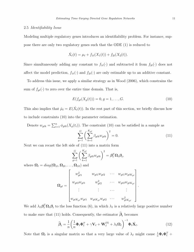
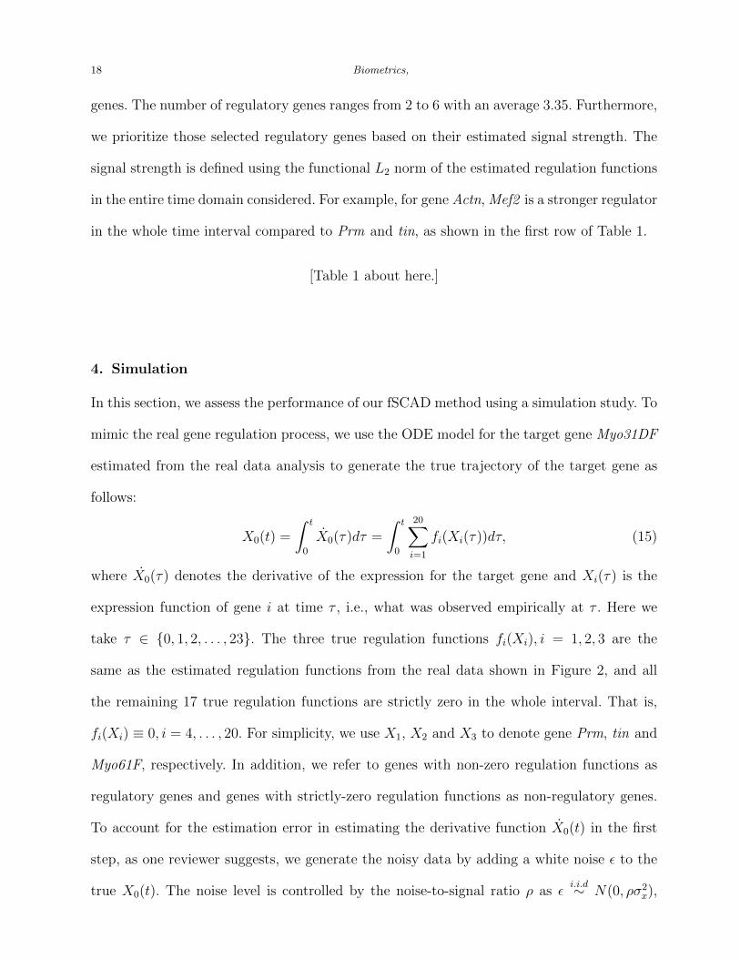
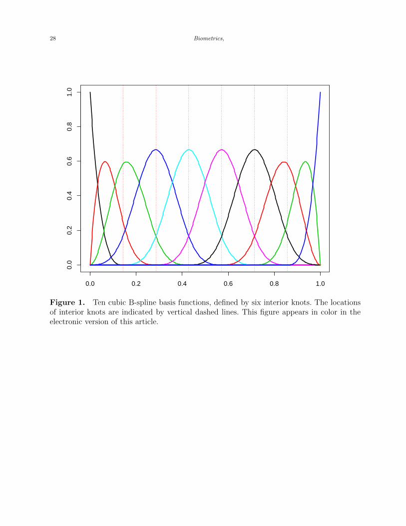
[Figure 1 about here.]
In this method, we choose B-spline basis functions due to their compact support property:
they are only nonzero in a local interval (de Boor, 2001). This property is crucial for the
computation efficiency and the sparse estimation of our fSCAD method. Figure 1 shows an
example of the ten cubic B-spline basis functions, defined by six interior knots. We can see
that each of the six basis functions in the center is nonzero over four adjacent sub-intervals.
6 Biometrics,
In addition, the three left-most basis functions and the three right-most basis functions are
nonzero over no more than four adjacent sub-intervals.
The method proposed in the rest of this section is trying to achieve the following three
tasks simultaneously: detecting those significant regulatory genes whose regulation function
fg`(Xg) 6= 0, identifying the nonzero intervals, Sg`, of these regulation functions and estimat-
ing the nonlinear regulation function, i.e., fg`(Xg), in the corresponding nonzero intervals.
2.2 Sparsity Penalty
The most common way to achieve sparsity is to add a penalty term to the loss function.
Our method belongs to this fashion by carefully choosing the penalty composition. Generally
speaking, the main idea is to first partition each regulatory gene’s whole expression domain
into several subintervals. The penalty term depends on the magnitude of the regulation effect
in each subinterval instead of in the entire expression domain.
The functional SCAD method was first proposed by Lin et al. (2016), which could be
considered as a functional generalization of the SCAD (Fan et al., 2004). In Lin et al. (2016),
they used fSCAD to estimate the coefficient function in the functional linear regression.
However, they only had one functional predictor in their model, and did not consider the
variable selection problem. In our work, we extend this method to do the variable selection
in the high-dimensional differential equation model. At the same time, we use the fSCAD
method to identify the nonzero intervals, Sg`, of these regulation functions and estimate
the nonlinear regulation function in the estimated nonzero intervals simultaneously. Now we
introduce our fSCAD penalty as follows.
The fSCAD penalty in our model is defined as
G∑g=1
Mg`
∆xg
∫ xgu
xgl
pλ(|fg`(Xg)|)dXg,
where xgl and xgu are the lower and upper bounds of the expression of the g-th gene Xg(t),
t ∈ [0, T ], ∆xg = xgu − xgl, and Mg` is the number of subintervals partitioned by the knots
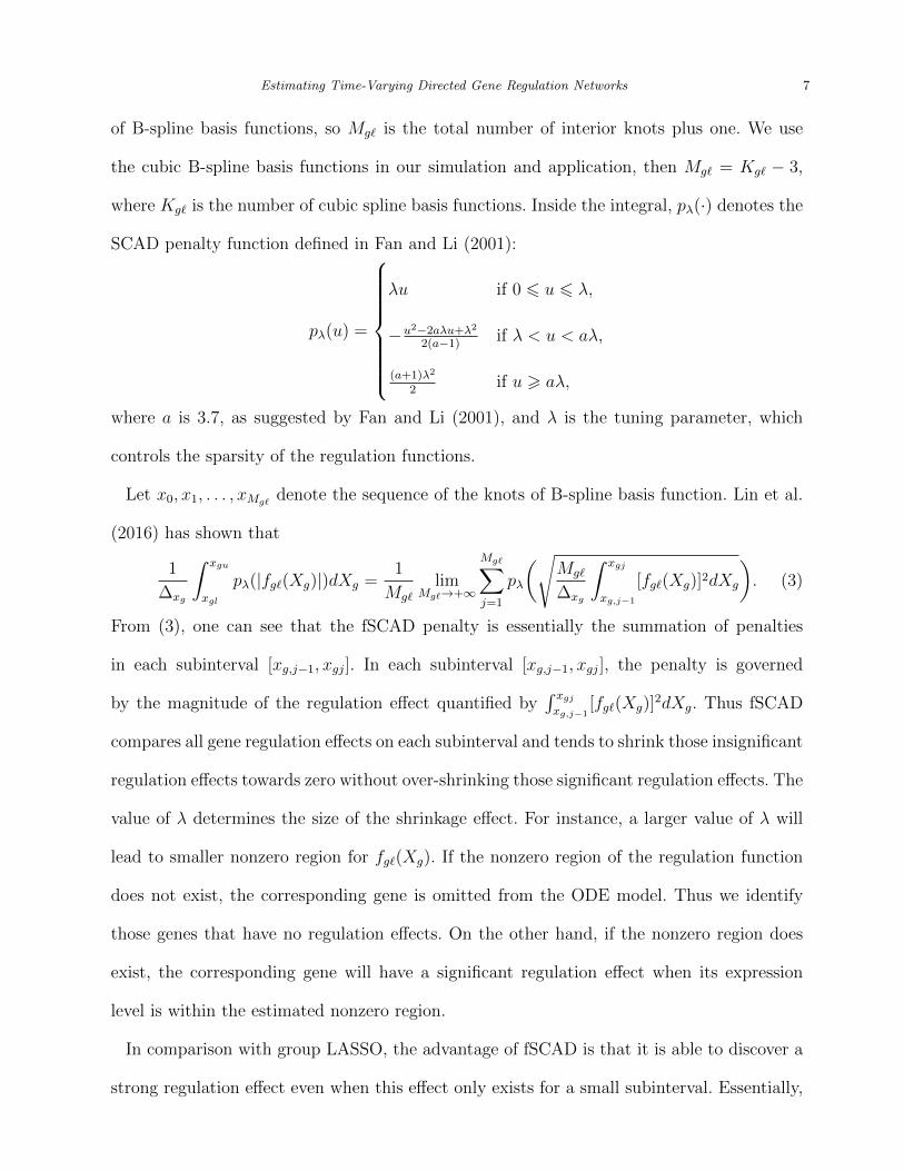
Estimating Time-Varying Directed Gene Regulation Networks 7
of B-spline basis functions, so Mg` is the total number of interior knots plus one. We use
the cubic B-spline basis functions in our simulation and application, then Mg` = Kg` − 3,
where Kg` is the number of cubic spline basis functions. Inside the integral, pλ(·) denotes the
SCAD penalty function defined in Fan and Li (2001):
pλ(u) =
λu if 0 6 u 6 λ,
−u2−2aλu+λ22(a−1) if λ < u < aλ,
(a+1)λ2
2if u > aλ,
where a is 3.7, as suggested by Fan and Li (2001), and λ is the tuning parameter, which
controls the sparsity of the regulation functions.
Let x0, x1, . . . , xMg`denote the sequence of the knots of B-spline basis function. Lin et al.
(2016) has shown that
1
∆xg
∫ xgu
xgl
pλ(|fg`(Xg)|)dXg =1
Mg`
limMg`→+∞
Mg`∑j=1
pλ
(√Mg`
∆xg
∫ xgj
xg,j−1
[fg`(Xg)]2dXg
). (3)
From (3), one can see that the fSCAD penalty is essentially the summation of penalties
in each subinterval [xg,j−1, xgj]. In each subinterval [xg,j−1, xgj], the penalty is governed
by the magnitude of the regulation effect quantified by∫ xgjxg,j−1
[fg`(Xg)]2dXg. Thus fSCAD
compares all gene regulation effects on each subinterval and tends to shrink those insignificant
regulation effects towards zero without over-shrinking those significant regulation effects. The
value of λ determines the size of the shrinkage effect. For instance, a larger value of λ will
lead to smaller nonzero region for fg`(Xg). If the nonzero region of the regulation function
does not exist, the corresponding gene is omitted from the ODE model. Thus we identify
those genes that have no regulation effects. On the other hand, if the nonzero region does
exist, the corresponding gene will have a significant regulation effect when its expression
level is within the estimated nonzero region.
In comparison with group LASSO, the advantage of fSCAD is that it is able to discover a
strong regulation effect even when this effect only exists for a small subinterval. Essentially,

8 Biometrics,
fSCAD penalizes the gene regulation function based on their regulation effects on each
subinterval, whereas group LASSO cannot achieve this because its penalty depends on the
regulation effect in the whole interval. For instance, if the regulation effect of one gene only
exists in a short interval, group LASSO will still shrink the effect to zero and ignore its
regulation effect completely even though the magnitude of the regulation effect is quite large
in that short interval.
2.3 Roughness Penalty
We assume that the regulation function fg`(Xg) is a smooth function of Xg because the
regulation effect is not expected to change dramatically when the regulatory gene’s expression
has a small change.
In order to obtain a smooth regulation function, we introduce a roughness penalty. For a
certain regulatory gene Xg, we define the roughness penalty as:∣∣∣∣∣∣∣∣df 2g`(Xg(t))
dt2
∣∣∣∣∣∣∣∣2 =
∫ T
0
(d2fg`(Xg(t))
dt2
)2
dt.
Based on the basis function expansion for the regulation function fg`(Xg(t)) defined in (2),
one can show that the second derivative of fg`(Xg(t)) can be calculated as
d2fg`(Xg(t))
dt2=
Kg`∑k=1
βg`kd2φg`k(Xg(t))
dt2=
Kg`∑k=1
βg`kdg`k,
where
dg`k =d2φg`k(Xg(t))
dt2=d2φg`kdX2
g
(dXg
dt
)2
+dφg`kdXg
d2Xg
dt2. (4)
The roughness penalty for all G regulation functions is given as
R` =G∑g=1
∣∣∣∣∣∣∣∣df 2g`(Xg(t))
dt2
∣∣∣∣∣∣∣∣2 =G∑g=1
∫ T
0
( Kg`∑k=1
βg`kdg`k
)2
dt. (5)

Estimating Time-Varying Directed Gene Regulation Networks 9
2.4 Parameter Estimation
Combining the fSCAD penalty (3) and the roughness penalty (5), we estimate fg`(Xg) via
minimizing the following loss function:
Q(β`) =1
n
n∑i=1
(X`(ti)−
G∑g=1
fg`(Xg(ti))
)2
+ γG∑g=1
∣∣∣∣∣∣∣∣df 2g`(Xg(t))
dt2
∣∣∣∣∣∣∣∣2
+G∑g=1
Mg`
∆xg
∫ xgu
xgl
pλ(|fg`(Xg)|)dXg, (6)
where β` = (βT1`,βT2`, . . . ,β
TG`)
T , is a length GK column vector of all basis function coeffi-
cients.
The first term in (6) quantifies the goodness of fit to the derivative. The second term is the
summation of the roughness penalty for each regulation function, and γ is the smoothing pa-
rameter which controls the smoothness of all regulation functions. The last term corresponds
to the fSCAD penalty.
For simplicity, we recast each part of the loss function in (6) into a matrix form. Following
the notations in (2), the first term of the loss function can be expressed as
1
n
n∑i=1
(X`(ti)−
G∑g=1
fg`(Xg(ti))
)2
=1
n(X` −ΦT
` β`)T (X` −ΦT
` β`), (7)
where X` = (X`(t1), X`(t2), . . . , X`(tn))T is a length n column vector, Φ` = [Φ1`n,Φ2`n, · · · ,ΦG`n]T
is a GK × n matrix,
Φg`n = [φg`(Xg(t1)),φg`(Xg(t2)), . . . ,φg`(Xg(tn))] is a Kg` × n matrix, and
φg`(Xg(t1)) =
(φg`1(Xg(t1)), φg`2(Xg(t1)), . . . , φg`Kg`
(Xg(t1))
)T. Let Vg` be a Kg` × Kg`
matrix with entries υg,ij =∫ T0dg`idg`jdx, where 1 6 i, j 6 Kg` and dg`i is expressed using
(4).
Let V` = diag(V1`,V2`, . . . ,VG`) be a matrix (GKg`×GKg`) with blocks V1`,V2`, . . . ,VG`
in its main diagonal and zeros elsewhere. Then the roughness penalty in (6) is transformed
into the following form:
γG∑g=1
∣∣∣∣∣∣∣∣df 2g`(Xg(t))
dt2
∣∣∣∣∣∣∣∣2 = γβT` V`β`. (8)

10 Biometrics,
Based on (3), the fSCAD penalty can be approximated as
Mg`
∆xg
∫ xgu
xgl
pλ(|fg`(Xg)|)dXg ≈Mg`∑j=1
pλ
(√Mg`
∆xg
∫ xgj
xg,j−1
[fg`(Xg)]2dXg
).
In addition, we define
||fg`[j]||22def=
∫ xgj
xg,j−1
[fg`(Xg)]2dXg = βTg`Mg`jβg`,
where Mg`j is a Kg` × Kg` matrix with entries mg`j,uv =∫ xgjxg,j−1
φg`u(Xg)φg`v(Xg)dXg, if
j 6 u, v 6 j+d and zero otherwise. Using the local quadratic approximation (LQA) proposed
in Fan and Li (2001), given some initial estimate β(0)g` , we can derive that
Mg`
∆xg
∫ xgu
xgl
pλ(|fg`(Xg)|)dXg ≈ βTg`W(0)g` βg` +G(β
(0)g` ),
where
W(0)g` =
1
2
Mg`∑j=1
(pλ(||fg`[j]||2
√Mg`/∆xg)
||fg`[j]||2√
∆xg/Mg`
Mglj
),
and
G(β(0)g` ) ≡
Mg`∑j=1
pλ
(||fg`[j]||2√∆xg/Mg`
)− 1
2
Mg`∑j=1
pλ
(||fg`[j]||2√∆xg/Mg`
)||fg`[j]||2√∆xg/Mg`
.
Adding all the fSCAD penalty for each gene, we have
G∑g=1
Mg`
∆xg
∫ xgu
xgl
pλ(|fg`(Xg)|)dXg ≈ βT` W(0)` β` +
G∑g=1
G(β(0)` ), (9)
where W(0)` = diag(W
(0)1` ,W
(0)2` , . . . ,W
(0)G`). Putting (7), (8) and (9) together, we obtain
Q(β`) =1
n(X` −ΦT
` β`)T (X` −ΦT
` β`) + γβT` V`β` + βT` W(0)` β` +
G∑g=1
G(β(0)g` ).
By minimizing Q(β`), we obtain the estimate for the basis coefficients
β` =1
n
(1
nΦ`Φ
T` + γV` + W
(0)`
)−1Φ`X`.
Then we can plug the estimate, β`, into (2) to obtain the estimates for all regulation
functions:
fg`(Xg) = φTg`(Xg)βg`, g = 1, . . . , G, ` = 1, . . . , G.
Estimating Time-Varying Directed Gene Regulation Networks 11
2.5 Identifiability Issue
Modeling multiple regulatory genes introduces an identifiability problem. For instance, sup-
pose there are only two regulatory genes such that the ODE (1) is reduced to
X`(t) = µ` + f1`(X1(t)) + f2`(X2(t)).
Since simultaneously adding any constant to f1`(·) and subtracted it from f2`(·) does not
affect the model prediction, f1`(·) and f2`(·) are only estimable up to an additive constant.
To address this issue, we apply a similar strategy as in Wood (2006), which constrains the
sum of fg`(·) to zero over the entire time domain. That is,
E(fg`(Xg(t))) = 0, g = 1, . . . , G. (10)
This also implies that µ` = E(X`(t)). In the rest part of this section, we briefly discuss how
to include constraints (10) into the parameter estimation.
Denote wg`k =∑n
i=1 φg`k(Xg(ti)). The constraint (10) can be satisfied in a sample as
G∑g=1
( Kg`∑k=1
βg`kwg`k
)2
= 0. (11)
Next we can recast the left side of (11) into a matrix form
G∑g=1
( Kg`∑k=1
βg`kwg`k
)2
= βT` Ω`β`,
where Ω` = diag(Ω1`,Ω2`, . . . ,ΩG`) and
Ωg` =
w2g`1 wg`1wg`2 · · · wg`1wg`Kg`
wg`2wg`1 w2g`2 · · · wg`2wg`Kg`
...... · · · ...
wg`Kg`wg`1 wg`Kg`
wg`2 · · · w2g`Kg`
.
We add λIβT` Ω`β` to the loss function (6), in which λI is a relatively large positive number
to make sure that (11) holds. Consequently, the estimator β` becomes
β` =1
n
(1
nΦ`Φ
T` + γV` + W
(0)` + λIΩ`
)−1Φ`X`. (12)
Note that Ω` is a singular matrix so that a very large value of λI might cause 1nΦ`Φ
T` +
12 Biometrics,
γV` + W(0)` + λIΩ` in (12) to be almost singular. If that is the case, we recommend to try
a new value of λI , for instance, half of the previous value.
Below we give the details of our algorithm to compute the estimated coefficients β`:
Step 1: Compute the initial estimate β(0)
` = 1n
(1nΦ`Φ
T` + λIΩ`
)−1Φ`X`.
Step 2: In each iteration, given β(i)
` , compute the corresponding W(i)` . Then β
(i+1)
` =
1n
(1nΦ`Φ
T` + γV` +W
(i)` + λIΩ`
)−1Φ`X`. If a variable is very small in magnitude
such that it makes
(1nΦ`Φ
T` + γV` +W
(i)` + λIΩ`
)almost singular or badly scaled
so that inverting
(1nΦ`Φ
T` + γV` + W
(i)` + λIΩ`
)is unstable, then we manually
shrink it into zero.
Step 3: Repeat Step 2 until β(i)` converges.
2.6 Choose Tuning parameters
We need to specify four tuning parameters in (12): the total number of basis functions used to
represent each regulation function, Kg`; the smoothing parameter in the roughness penalty
for each regulation function, γ; the fSCAD penalty for sparsity, λ; and the identifiability
parameter, λI .
First of all, a large value of Kg` is chosen to obtain a good approximation for each regulation
function fg`(·). This will not result in a saturated model since the smoothing parameter, γ,
and fSCAD penalty parameter, λ, will control the roughness of the regulation functions.
Second, λI ∈ [104, 109] generally works well according to our experience and this choice is
not crucial. We note that the value of λI only affects the convergence speed. Once Kg` and
λI are determined, one can use a popular selection criterion such as information criterion
(AICc, BIC) or cross validation to search the optimal values for γ and λ on a discrete grid.
Our experience from the real data application suggests that the AICc information criterion
tends to work well from a practical perspective.

Estimating Time-Varying Directed Gene Regulation Networks 13
2.7 Derivative Estimation
The ODE model in (1) uses the derivatives of each gene as the response. In this section, we
introduce a smoothing spline method to estimate the derivative of each gene based on the
its own observed expression values. Other methods for the derivative estimation can also be
used in our framework.
Let Yi denote the measurement for a particular gene at time ti, ti ∈ [0, T ]. Suppose that
Yi, i = 1, . . . , n, is from an unknown gene expression function X(t). That is,
Yi = X(ti) + εi, i = 1, . . . , n,
where εi is independently and identically distributed from a normal distribution N(0, σ2s).
Our goal is to estimate X(t) and X(t) from Yi, i = 1, . . . , n.
We first represent X(t) using a linear combination of B-spline basis functions:
X(t) =J∑j=1
θiψj(t) = ψ(t)Tθ,
in which θ is the length J vector of coefficients, and ψ(t) is the length J vector of basis
functions. Then we estimate the vector of coefficients θ by minimizing the following loss
function:
Q0(θ) =n∑i=1
(Yi −X(ti)
)2
+ λ0
∫ [X(t)
]2dt, λ0 > 0. (13)
Intuitively, the first term in Q0(θ) quantifies the goodness of fit to the data, and the second
one controls the roughness of the estimated function. The relative importance between these
two terms is controlled by λ0. For instance, a larger value of λ0 will lead to a smoother
estimate for X(t). Here we suggest using the generalized cross validation (GCV) score in
Wahba and Craven (1978) to determine the value of λ0.
To estimate the vector of the basis coefficients θ, we can rewrite (13) into a matrix form:
Q0(θ) = (Y−Ψθ)T (Y−Ψθ) + λ0θTRθ,
where R is a J × J matrix with entries Rij =∫ψi(t)ψj(t)dt and Ψ is an n× J matrix with
14 Biometrics,
entries Ψij = ψj(ti). Taking the derivative Q0(θ) with respect to θ, one can obtain
θ = (ΨTΨ + λ0R)−1ΨTY.
Thus, the estimated trajectory for X(t) and the derivative X(t) can be expressed as X(t) =
ψ(t)T θ and ˆX(t) = ψ(t)T θ.
Because the estimated derivatives for gene ` at observed time points are essentially corre-
lated across time, equation (7) should take this correlation into consideration and be replaced
by
1
n( ˆX` −ΦT
` β`)T[Cov( ˆX)
]−1( ˆX` −ΦT
` β`),
where the estimated variance-covariance matrix of the derivatives Cov( ˆX) can be obtained
with the delta method,
Cov( ˆX) = ΨT
Cov(θ)Ψ = σ2sΨ
T(ΨTΨ + λ0R)−1ΨTΨ(ΨTΨ + λ0R)−1Ψ, (14)
in which ˆX = ( ˆX(t1), . . . ,ˆX(tn))T , Ψ is a n × J matrix with entries ψj(ti) and σ2
s can be
obtained by computing the sample variance of the residuals es = Y−Ψθ.
In fact, as one reviewer suggests, our proposed algorithm given at the end of Section 2.5
is still applicable by simply letting[Cov( ˆX)
]−1= LT
` L` be the Cholesky decomposition of
the inverse variance-covariance matrix and then pre-conditioning both ˆX` and ΦT` with L`.
Consequently, equation (12) becomes
β` =1
n
(1
nΦ`L
T` L`Φ
T` + γV` + W
(0)` + λIΩ`
)−1Φ`L
T` L`
ˆX`.
3. Application
We consider a data set of 20 Drosophila melanogaster genes involved in the muscle develop-
ment during the embryonic stage (see Bar-Joseph (2004) for details). The time-course gene
expressions are measured at 30 time points in the embryonic stage (Arbeitman et al., 2002).
The time-varying directed gene regulation network of these 20 genes are modeled using
the nonlinear ODE model (1). The time-varying regulation functions fg`(Xg) in (1) for each
Estimating Time-Varying Directed Gene Regulation Networks 15
of those 20 genes are estimated in two steps. In the first step, we obtain the estimate for the
trajectory of each gene and its derivatives using the smoothing spline method, as introduced
in Section 2.7. In the second step, we treat the derivative estimates for each gene as the
response and all genes’ trajectory estimates as the covariates in ODE model (1). We then
estimate the basis coefficients for each regulation function via (12). The smoothing parameter
γ and the sparsity parameter λ are both determined simultaneously using AICc criterion.
The smoothing parameter γ is chosen from four candidate values: 10−5, 10−3, 10−1, and 10.
The sparsity parameter λ is selected from five candidate values: 10−2, 10−1, 1, and 10. Since
the results are not sensitive to specific values of the number of basis functions, Kg`, and the
identifiability parameter, λI , we set their values to be Kg` = 5 and λI = 104 to ease the
computation.
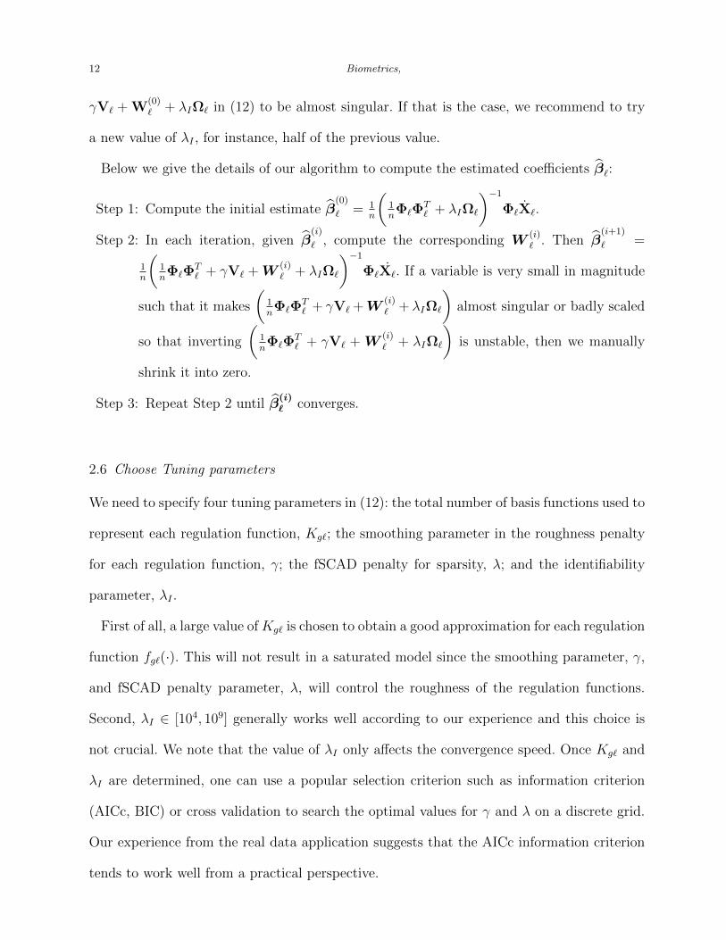
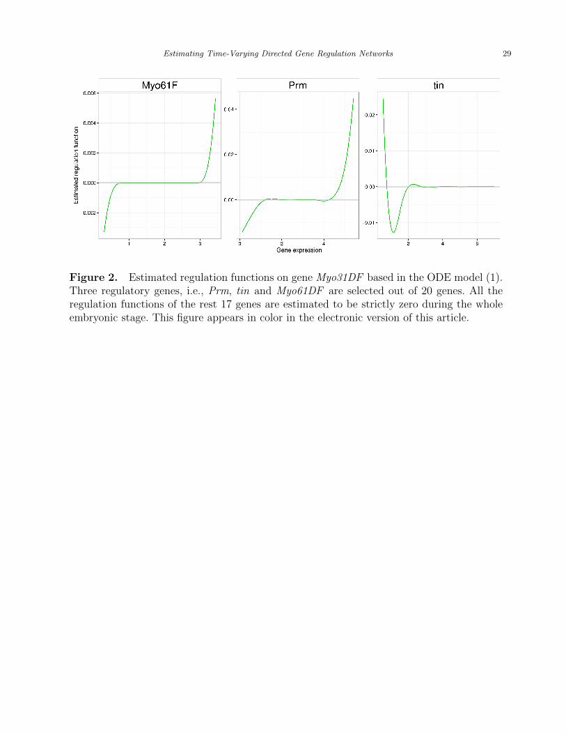
[Figure 2 about here.]
Figure 2 shows the estimated regulation functions for gene Myo31DF. It can be seen that 3
out of 20 genes are selected, which means that the regulation functions of the other 17 genes
are estimated to be strictly zero during the entire embryonic stage. Those three estimated
regulation functions shown in Figure 2 all have non-linear trends and show local sparsity to
some extent.
We compare the prediction performance of our proposed method with the group Lasso
method in the real data application. To be more specific, we remove the last observation for
all genes in the network and estimate the regulation functions for the target gene Myo31DF
using the remaining observations only. Then we use our method and the group Lasso method
to estimate the gene regulation functions in the ODE model (1). We then use the estimated
ODE model (1) to predict the expression of the target gene at the last time point. We
also compare their prediction performances with two other methods: the constant expression
method and an autoregressive model, AR1. The constant expression model simply takes the

16 Biometrics,
sample mean from previously observed trajectories values of Myo31DF as the prediction
value. The AR1 method is fitted using the maximum likelihood approach. The detailed
results, presented in Web Table 1 in the supplementary file, show that the locally sparse
method has the most accurate prediction among all methods.
To check whether our finding for gene Myo31DF makes biology sense, we conduct a
literature search for studies on gene interactions using the Drosophila Interactions Database
(Murali et al., 2011) and the GeneMANIA tool (Warde-Farley et al., 2010). We find evidences
in the literature about all three regulatory genes Myo61F, Prm, and tin on gene Myo31DF.
For instance, Hozumi et al. (2006) suggested that both Myo61F and Myo31DF played
a crucial role in generating left-right asymmetry of the embryonic gut. They found that
Myo31DF was required in the hindgut epithelium for normal embryonic handedness and the
overexpression of Myo61F reversed the handedness of the embryonic gut, and its knockdown
also caused a left-right patterning defect. These two unconventional myosin I proteins might
have antagonistic functions in left-right patterning. The results obtained from our analysis
match these insights. For instance, Figure 2 shows that gene Myo61F only regulates gene
Myo31DF when its expression level is either less than 1 or greater than 2. Thus, either the
knockdown or overexpression of Myo61F will cause a left-right patterning defect. In addition,
Lewis, Burge, and Bartel (2005), Ruby et al. (2007), Ruby, Jan, and Bartel (2007) and
Kheradpour et al. (2007) suggested that gene Prm and gene Myo31DF shared two common
miRNAs, i.e., mir-iab-4 and mir-999. As for gene tin, even though there was no direct
evidence showing its regulation effect on Myo31DF, Fu et al. (1997) found out that tin was
critical in determining the patterning of the Drosophila heart. Because of gene Myo31DF ’s
role in generating the left-right asymmetry gut, our hypothesis is that tin regulates Myo31DF
to insure the left-right asymmetry formation in the heart. This hypothesis needs to be further
investigated in real genetic studies.

Estimating Time-Varying Directed Gene Regulation Networks 17
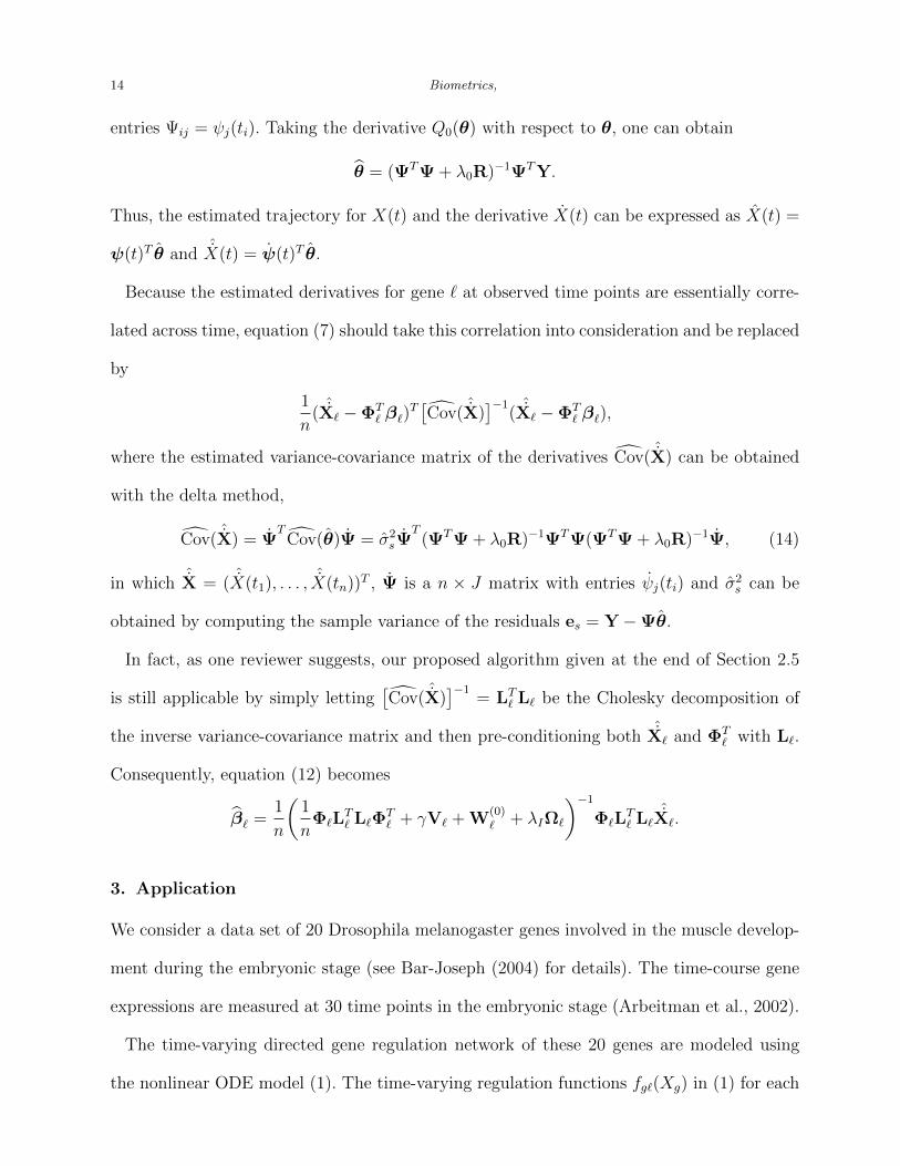
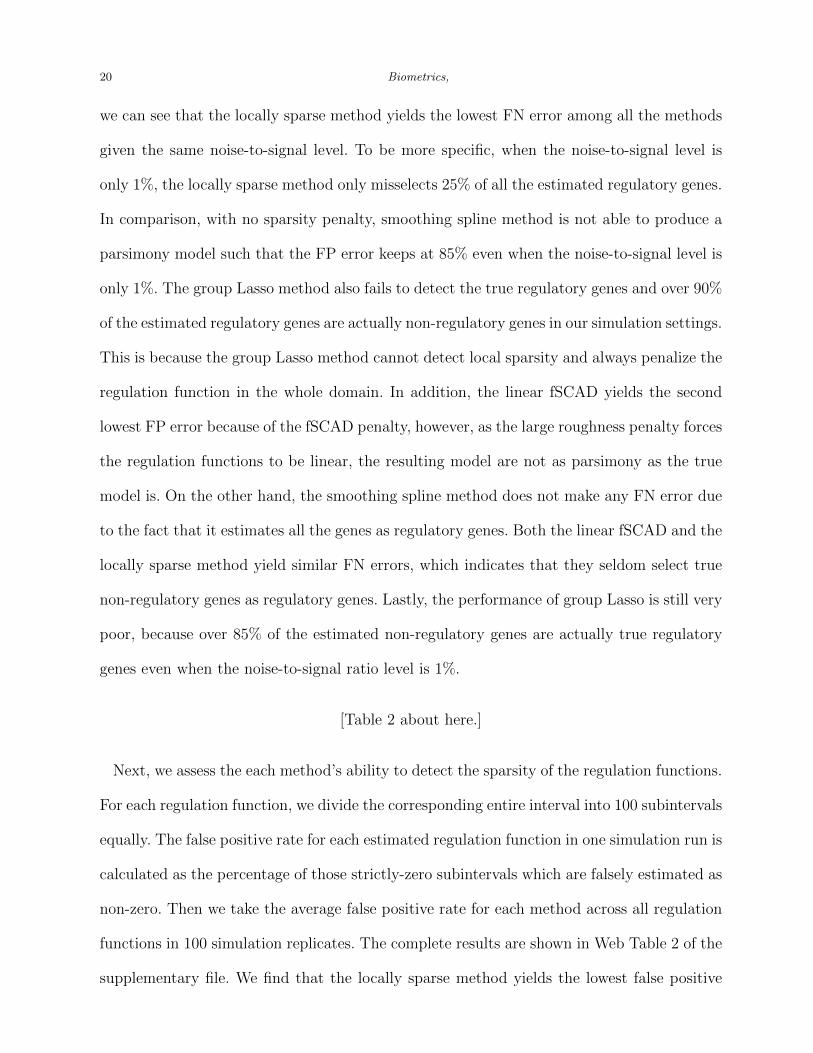
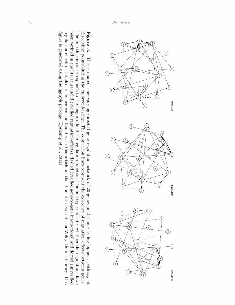
[Figure 3 about here.]
Once the regulation functions for all 20 genes are estimated, we can visualize the whole
GRN at any given time point. Figure 3 shows the estimated GRN at different selected time
points during the embryonic stage. One important feature of the estimated GRN is that
the regulation effects between genes are time-varying. For example, Prm regulates sls at the
beginning of the embryonic stage, i.e., t = 3h, however, Mef2 replace Prm’s role in regulating
sls in the middle stage. In addition, from the whole network point of view, we observe that
genes interact with each other more frequently in the beginning than in the middle or at the
end of the embryonic stage. Finally, we find some strong regulators such as Mef2, Myo61F,
Prm and Mhc, which act as hubs in our estimated GRN.
In Figure 3, we highlight those interactions that have been verified in the literature. Details
of the references for each interaction are provided in the supplementary materials. A solid
line indicates the corresponding directed regulation effect between genes has been verified;
a dashed line means the corresponding gene-to-gene interaction has been discovered before
but the exactly direction is unclear; and a dotted line means the corresponding interaction
has not been found so far. Most regulation effects estimated using our method have been
verified previously. Those regulation effects that have not been discovered may be candidate
hypotheses for future investigation. It is worth mentioning that the total number of known
interactions in the literature is 158 out of 400 possible interactions. In other words, the
background interaction rate is 39.5%(=158/400). Using our method, wIt is woe estimate 67
interactions, 58 of which are verified in the literature. The discovery rate for our method is
86.6%(=58/67), which is more than twice the background interaction rate.
Another very important feature of our estimated GRN shown in Figure 3 is that the
estimated network is sparsely connected. In other words, only a limited number of genes
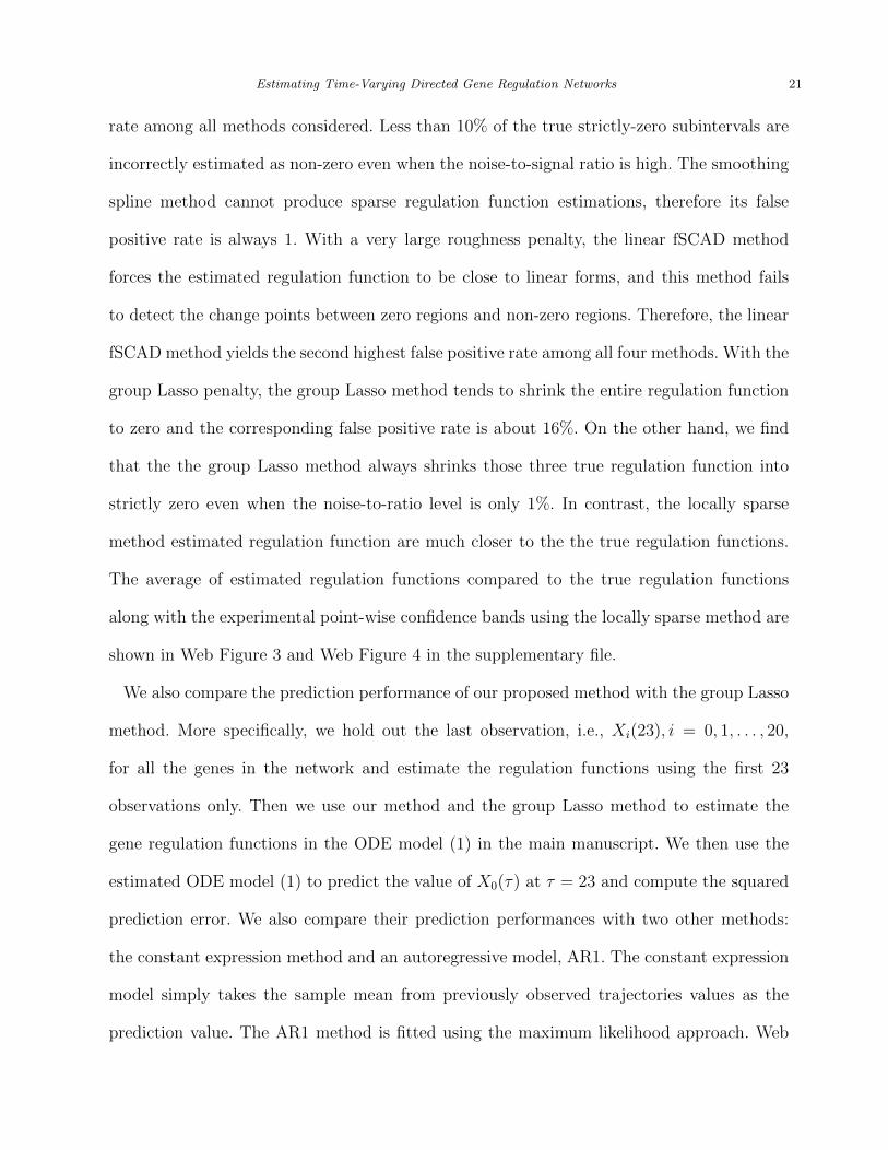
regulate a target gene. Table 1 displays a complete list of estimated regulatory genes for all
18 Biometrics,
genes. The number of regulatory genes ranges from 2 to 6 with an average 3.35. Furthermore,
we prioritize those selected regulatory genes based on their estimated signal strength. The
signal strength is defined using the functional L2 norm of the estimated regulation functions
in the entire time domain considered. For example, for gene Actn, Mef2 is a stronger regulator
in the whole time interval compared to Prm and tin, as shown in the first row of Table 1.
[Table 1 about here.]
4. Simulation
In this section, we assess the performance of our fSCAD method using a simulation study. To
mimic the real gene regulation process, we use the ODE model for the target gene Myo31DF
estimated from the real data analysis to generate the true trajectory of the target gene as
follows:
X0(t) =
∫ t
0
X0(τ)dτ =
∫ t
0
20∑i=1
fi(Xi(τ))dτ, (15)
where X0(τ) denotes the derivative of the expression for the target gene and Xi(τ) is the
expression function of gene i at time τ , i.e., what was observed empirically at τ . Here we
take τ ∈ 0, 1, 2, . . . , 23. The three true regulation functions fi(Xi), i = 1, 2, 3 are the
same as the estimated regulation functions from the real data shown in Figure 2, and all
the remaining 17 true regulation functions are strictly zero in the whole interval. That is,
fi(Xi) ≡ 0, i = 4, . . . , 20. For simplicity, we use X1, X2 and X3 to denote gene Prm, tin and
Myo61F, respectively. In addition, we refer to genes with non-zero regulation functions as
regulatory genes and genes with strictly-zero regulation functions as non-regulatory genes.
To account for the estimation error in estimating the derivative function X0(t) in the first
step, as one reviewer suggests, we generate the noisy data by adding a white noise ε to the
true X0(t). The noise level is controlled by the noise-to-signal ratio ρ as εi.i.d∼ N(0, ρσ2
x),
Estimating Time-Varying Directed Gene Regulation Networks 19
where σx is the sample standard deviation of the true trajectory X0(t) empirically observed
at τ ∈ 0, 1, 2, . . . , 23.
We estimate ODE model (1) using the group Lasso method and the following three
methods:
Locally sparse method: the loss function defined in (7) with both fSCAD penalty and
roughness penalty;
Smoothing spline method: the loss function defined in (7) with roughness penalty only,
i.e., λ = 0;
Linear fSCAD method: the loss function defined in (7) with the fSCAD penalty and
a very large roughness penalty. More specifically, we fix γ = 100 to force the estimated
regulation functions to be almost linear.
For the locally sparse method and the smoothing spline method, the smoothing parameter γ
is chosen from four candidate values: 10, 10−1, 10−3 and 10−5 using AICc. For both the locally
sparse method and the linear fSCAD method, the sparsity parameter λ is selected from five
candidate values: 10, 1, 10−1 and 10−2 using AICc. In addition, the number of basis function
Kg` and the identifiability parameter λI remain the same as in the real data analysis, i.e.,
Kg` = 5 and λI = 104. For the group Lasso method, we use the 5-fold cross-validation to
choose the penalty parameter.
We access the variable-selection accuracy for each method using the false negative error
(FN) and the false positive error (FP), which are defined in the gene regulation scenario as
follows:
FN =# of incorrectly estimated non-regulatory genes
# of all true regulatory genes,
FP =# of incorrectly estimated regulatory gene
# of all estimated regulatory gene.
The simulation is repeated for 100 times and the results are presented in Table 2. First of all,
20 Biometrics,
we can see that the locally sparse method yields the lowest FN error among all the methods
given the same noise-to-signal level. To be more specific, when the noise-to-signal level is
only 1%, the locally sparse method only misselects 25% of all the estimated regulatory genes.
In comparison, with no sparsity penalty, smoothing spline method is not able to produce a
parsimony model such that the FP error keeps at 85% even when the noise-to-signal level is
only 1%. The group Lasso method also fails to detect the true regulatory genes and over 90%
of the estimated regulatory genes are actually non-regulatory genes in our simulation settings.
This is because the group Lasso method cannot detect local sparsity and always penalize the
regulation function in the whole domain. In addition, the linear fSCAD yields the second
lowest FP error because of the fSCAD penalty, however, as the large roughness penalty forces
the regulation functions to be linear, the resulting model are not as parsimony as the true
model is. On the other hand, the smoothing spline method does not make any FN error due
to the fact that it estimates all the genes as regulatory genes. Both the linear fSCAD and the
locally sparse method yield similar FN errors, which indicates that they seldom select true
non-regulatory genes as regulatory genes. Lastly, the performance of group Lasso is still very
poor, because over 85% of the estimated non-regulatory genes are actually true regulatory
genes even when the noise-to-signal ratio level is 1%.
[Table 2 about here.]
Next, we assess the each method’s ability to detect the sparsity of the regulation functions.
For each regulation function, we divide the corresponding entire interval into 100 subintervals
equally. The false positive rate for each estimated regulation function in one simulation run is
calculated as the percentage of those strictly-zero subintervals which are falsely estimated as
non-zero. Then we take the average false positive rate for each method across all regulation
functions in 100 simulation replicates. The complete results are shown in Web Table 2 of the
supplementary file. We find that the locally sparse method yields the lowest false positive
Estimating Time-Varying Directed Gene Regulation Networks 21
rate among all methods considered. Less than 10% of the true strictly-zero subintervals are
incorrectly estimated as non-zero even when the noise-to-signal ratio is high. The smoothing
spline method cannot produce sparse regulation function estimations, therefore its false
positive rate is always 1. With a very large roughness penalty, the linear fSCAD method
forces the estimated regulation function to be close to linear forms, and this method fails
to detect the change points between zero regions and non-zero regions. Therefore, the linear
fSCAD method yields the second highest false positive rate among all four methods. With the
group Lasso penalty, the group Lasso method tends to shrink the entire regulation function
to zero and the corresponding false positive rate is about 16%. On the other hand, we find
that the the group Lasso method always shrinks those three true regulation function into
strictly zero even when the noise-to-ratio level is only 1%. In contrast, the locally sparse
method estimated regulation function are much closer to the the true regulation functions.
The average of estimated regulation functions compared to the true regulation functions
along with the experimental point-wise confidence bands using the locally sparse method are
shown in Web Figure 3 and Web Figure 4 in the supplementary file.
We also compare the prediction performance of our proposed method with the group Lasso
method. More specifically, we hold out the last observation, i.e., Xi(23), i = 0, 1, . . . , 20,
for all the genes in the network and estimate the regulation functions using the first 23
observations only. Then we use our method and the group Lasso method to estimate the
gene regulation functions in the ODE model (1) in the main manuscript. We then use the
estimated ODE model (1) to predict the value of X0(τ) at τ = 23 and compute the squared
prediction error. We also compare their prediction performances with two other methods:
the constant expression method and an autoregressive model, AR1. The constant expression
model simply takes the sample mean from previously observed trajectories values as the
prediction value. The AR1 method is fitted using the maximum likelihood approach. Web
22 Biometrics,
Table 3 shows that the locally sparse method yields the lowest mean squared prediction error
among all methods, which is only about 10% compared to the group Lasso method and the
AR1 model.
In summary, our proposed method can correctly select the true regulatory genes without
misselecting those true non-regulatory genes in the ODE model compared to other alternative
methods. In addition, it can also successfully identify the strictly-zero subregions of all
regulation functions. Finally, it outperforms popular method such as group Lasso in term of
the forward prediction accuracy.
5. Conclusions
ODE models are widely used to model a dynamical system in many fields such as biology,
economics, and physics. In this article, we use a high-dimensional nonlinear ODE model
to describe a time-varying direct GRN. It is worth mentioning, as one reviewer suggests,
the ODE model itself is time-stationary in the sense that all the regulation functions are
deterministic functions of the regulatory gene expressions, but the edges may implicitly
emerge or disappear over time, and the strength of the edge may vary with time, because
the expressions of regulatory genes change with time. We propose the fSCAD method to
estimate the unknown regulation functions in the high-dimensional ODE model from the
time-course gene expression data.
In the real data application, we show that our method can simultaneously detect the signif-
icant regulatory genes, estimate the nonlinear regulation functions without any parametric
assumption, and identify the intervals with no regulation effects. The resulting GRN with the
estimated regulation functions has many potential implications. First, based on the estimated
edges and their corresponding directions, new hypotheses for gene regulation mechanism can
be proposed as candidate relationships for future investigations. For those edges that have
already been verified in the literature, we can prioritize them based on the estimated signal

Estimating Time-Varying Directed Gene Regulation Networks 23
strength. In addition, when no prior knowledge about the direction of the regulation effect is
available, our method can be a good starting point for the direction detection. Furthermore,
our method can not only suggest potentially unverified regulation relationships between
genes, but also give clues in which time periods the regulation effects are most likely to
be detected. This advantage can greatly facilitate the future biology experiment designs for
detecting gene regulation effects.
Furthermore, our simulation study shows that our method is able to estimate the true
regulation functions under different levels of noises in the data more accurately in comparison
with the group Lasso method. Finally, our method avoids solving the ODEs numerically,
making it computational efficient and feasible in the high-dimensional context. Our method
can be extended to model and estimate other high-dimensional directed networks from time-
course or longitudinal data.
Acknowledgements
The authors are grateful for the invaluable comments and suggestions from the editor, Dr.
Yi-Hau Chen, an associate editor, and two reviewers. The authors also thank Prof. Eric
P. Xing and Prof. Le Song for kindly providing us the data and their computing codes.
This research was supported by Nie’s Postgraduate Scholarship-Doctorial (PGS-D) from the
Natural Sciences and Engineering Research Council of Canada (NSERC), and the NSERC
Discovery grants of Wang and Cao.
Supplementary Materials
Web Figures, Tables, and the reference details for gene interactions referenced in Sections
3 and 4 are available at the Biometrics website on Wiley Online Library. The R code is
available at https://github.com/YunlongNie/flyfuns.

24 Biometrics,
References
Arbeitman, M. N., Furlong, E. E., Imam, F., Johnson, E., Null, B. H., Baker, B. S., Krasnow,
M. A., Scott, M. P., Davis, R. W., and White, K. P. (2002). Gene expression during the
life cycle of drosophila melanogaster. Science 297, 2270–2275.
Bar-Joseph, Z. (2004). Analyzing time series gene expression data. Bioinformatics 20,
2493–2503.
Cao, J. and Zhao, H. (2008). Estimating dynamic models for gene regulation networks.
Bioinformatics 24, 1619–1624.
Chen, J. and Wu, H. (2008). Estimation of time-varying parameters in deterministic dynamic
models. Statistica Sinica 18, 987–1006.
de Boor, C. (2001). A Practical Guide to Splines. Applied Mathematical Sciences. Springer,
New York.
Epskamp, S., Cramer, A. O. J., Waldorp, L. J., Schmittmann, V. D., and Borsboom, D.
(2012). qgraph: Network visualizations of relationships in psychometric data. Journal of
Statistical Software 48, 1–18.
Fan, J. and Li, R. (2001). Variable selection via nonconcave penalized likelihood and its
oracle properties. Journal of the American Statistical Association 96, 1348–1360.
Fan, J., Peng, H., et al. (2004). Nonconcave penalized likelihood with a diverging number
of parameters. Annals of Statistics 32, 928–961.
Fu, Y., Ruiz-Lozano, P., and Evans, S. M. (1997). A rat homeobox gene, rnkx-2.5, is
a homologue of the tinman gene in drosophila and is mainly expressed during heart
development. Development Genes and Evolution 207, 352–358.
Hanneke, S., Fu, W., and Xing, E. P. (2010). Discrete temporal models of social networks.
Electronic Journal of Statistics 4, 585–605.
Hozumi, S., Maeda, R., Taniguchi, K., Kanai, M., Shirakabe, S., Sasamura, T., Speder,

Estimating Time-Varying Directed Gene Regulation Networks 25
P., Noselli, S., Aigaki, T., Murakami, R., et al. (2006). An unconventional myosin in
drosophila reverses the default handedness in visceral organs. Nature 440, 798–802.
Jensen, F. V. (1996). An introduction to Bayesian networks, volume 210. UCL Press, London.
Kheradpour, P., Stark, A., Roy, S., and Kellis, M. (2007). Reliable prediction of regulator
targets using 12 drosophila genomes. Genome research 17, 1919–1931.
Kolar, M., Song, L., Ahmed, A., and Xing, E. P. (2010). Estimating time-varying networks.
Annals of Applied Statistics 4, 94–123.
Kolar, M. and Xing, E. P. (2009). Sparsistent estimation of time-varying discrete markov
random fields. arXiv:0907.2337 .
Laubenbacher, R. and Stigler, B. (2004). A computational algebra approach to the reverse
engineering of gene regulatory networks. Journal of Theoretical Biology 229, 523–537.
Lewis, B., Burge, C., and Bartel, D. (2005). Conserved seed pairing, often flanked by
adenosines, indicates that thousands of human genes are microrna targets. Cell 120,
15.
Lin, Z., Cao, J., Wang, L., and Wang, H. (2016). Locally sparse estimator for func-
tional linear regression models. Journal of Computational and Graphical Statistics
doi:10.1080/10618600.2016.1195273, 1–41.
Lu, T., Liang, H., Li, H., and Wu, H. (2011). High-dimensional odes coupled with mixed-
effects modeling techniques for dynamic gene regulatory network identification. Journal
of the American Statistical Association 106, 1242–1258.
Luscombe, N. M., Babu, M. M., Yu, H., Snyder, M., Teichmann, S. A., and Gerstein,
M. (2004). Genomic analysis of regulatory network dynamics reveals large topological
changes. Nature 431, 308–312.
Mehra, S., Hu, W.-S., and Karypis, G. (2004). A boolean algorithm for reconstructing the
structure of regulatory networks. Metabolic Engineering 6, 326–339.
26 Biometrics,
Murali, T., Pacifico, S., Yu, J., Guest, S., Roberts, G. G., and Finley, R. L. (2011). Droid
2011: a comprehensive, integrated resource for protein, transcription factor, rna and gene
interactions for drosophila. Nucleic Acids Research 39, D736–D743.
Needham, C. J., Bradford, J. R., Bulpitt, A. J., and Westhead, D. R. (2007). A primer on
learning in bayesian networks for computational biology. PLoS Computational Biology
3, 129.
Ramsay, J. O. and Silverman, B. W. (2002). Applied functional data analysis: methods and
case studies, volume 77. Springer, New York.
Ruby, J. G., Jan, C. H., and Bartel, D. P. (2007). Intronic microrna precursors that bypass
drosha processing. Nature 448, 83–86.
Ruby, J. G., Stark, A., Johnston, W. K., Kellis, M., Bartel, D. P., and Lai, E. C. (2007).
Evolution, biogenesis, expression, and target predictions of a substantially expanded set
of drosophila micrornas. Genome research 17, 1850–1864.
Song, L., Kolar, M., and Xing, E. P. (2009). Keller: estimating time-varying interactions
between genes. Bioinformatics 25, i128–i136.
Steuer, R., Kurths, J., Daub, C. O., Weise, J., and Selbig, J. (2002). The mutual information:
detecting and evaluating dependencies between variables. Bioinformatics 18, S231–S240.
Stuart, J. M., Segal, E., Koller, D., and Kim, S. K. (2003). A gene-coexpression network for
global discovery of conserved genetic modules. Science 302, 249–255.
Thomas, R. (1973). Boolean formalization of genetic control circuits. Journal of Theoretical
Biology 42, 563–585.
Wahba, G. and Craven, P. (1978). Smoothing noisy data with spline functions. estimating the
correct degree of smoothing by the method of generalized cross-validation. Numerische
Mathematik 31, 377–404.
Warde-Farley, D., Donaldson, S. L., Comes, O., Zuberi, K., Badrawi, R., Chao, P., Franz,
Estimating Time-Varying Directed Gene Regulation Networks 27
M., Grouios, C., Kazi, F., Lopes, C. T., et al. (2010). The genemania prediction
server: biological network integration for gene prioritization and predicting gene function.
Nucleic Acids Research 38, W214–W220.
Wood, S. (2006). Generalized additive models: an introduction with R. Chapman and
Hall/CRC, London.
Wu, H., Lu, T., Xue, H., and Liang, H. (2014). Sparse additive ordinary differential equations
for dynamic gene regulatory network modeling. Journal of the American Statistical
Association 109, 700–716.
Yuan, M. and Lin, Y. (2006). Model selection and estimation in regression with grouped
variables. Journal of the Royal Statistical Society: Series B (Statistical Methodology) 68,
49–67.
Zou, H. (2006). The adaptive lasso and its oracle properties. Journal of the American
Statistical Association 101, 1418–1429.
28 Biometrics,
0.0 0.2 0.4 0.6 0.8 1.0
0.0
0.2
0.4
0.6
0.8
1.0
Figure 1. Ten cubic B-spline basis functions, defined by six interior knots. The locationsof interior knots are indicated by vertical dashed lines. This figure appears in color in theelectronic version of this article.
Estimating Time-Varying Directed Gene Regulation Networks 29
Figure 2. Estimated regulation functions on gene Myo31DF based in the ODE model (1).Three regulatory genes, i.e., Prm, tin and Myo61DF are selected out of 20 genes. All theregulation functions of the rest 17 genes are estimated to be strictly zero during the wholeembryonic stage. This figure appears in color in the electronic version of this article.
30 Biometrics,
Fig
ure
3.
The
estimated
time-vary
ing
directed
gene
regulation
netw
orkof
20gen
esin
the
muscle
develop
men
tpath
way
atth
reetim
ep
oints
durin
gth
eem
bryon
icstage.
The
connection
lines
represen
tth
eex
istence
ofregu
lationeff
ectsb
etween
genes.
The
line
thick
ness
correspon
ds
toth
em
agnitu
de
ofth
eregu
lationfu
nction
.T
he
line
typ
ein
dicates
wheth
erth
eregu
lations
have
been
verified
inth
eliteratu
re:solid
(verified
regulation
effects),
dash
ed(verifi
edgen
e-to-gene
interaction
s)an
ddotted
(unverifi
edregu
lationeff
ects).D
etailedreferen
cecan
be
found
with
this
articleat
the
Biom
etricsw
ebsite
onW
ileyO
nlin
eL
ibrary.
This
figu
reis
generated
usin
gth
eqgrap
hpackage
(Epskam
pet
al.,2012).

Estimating Time-Varying Directed Gene Regulation Networks 31
Table 1The regulatory genes for all 20 genes selected by our method. The regulatory genes are sorted by their overall
regulation effect on the corresponding target gene. For example, Mef2 has the largest the overall regulation effect onActn in comparison with Prm and tin.
Target Gene Regulatory Genes
Actn Mef2 Prm tindpp Mef2 Prm flweve Myo61F Mef2 srp evefln tin Prm Actn Mhc Msp300 flwflw Myo61F Prmhow sls Mlc1 flnlmd srp Myo61F flwMef2 Myo61F up flw lmdMhc Msp300Mlc1 Msp300 Prm tinMsp300 tin up Mlc1 Prm Msp300Myo31DF Prm tin Myo61FMyo61F Msp300 tin flnPrm Msp300sls Prm tin how Mef2srp Mef2 Prm flw eve twi Msp300tin Mef2 lmd Myo61F flw twitwi Mef2 srpup Msp300 Prm Mlc1 flwwg Mef2 twi

32 Biometrics,
Table 2The means and standard deviations (SD) of the false positive errors (FP) and the false negative errors (FN) of the
four methods in 100 simulation replicates. Here ρ represents the noise-to-signal ratio in the simulated data.
FP FNMethod ρ Mean SD Mean SD
Locally Sparse 1% 25.0% 0.0% 0.0% 0.0%5% 30.0% 11.5% 9.0% 15.6%
Smoothing Spline 1% 85.0% 0.0% 0.0% 0.0%5% 85.0% 0.0% 0.0% 0.0%
Linear fSCAD 1% 63.9% 5.5% 4.8% 11.7%5% 63.9% 5.5% 4.8% 11.7%
Group Lasso 1% 94.9% 8.2% 88.1% 19.5%5% 99.5% 3.2% 99.3% 4.7%