estimating treatment effects from observational data … a mother reduce the birthweight of her ......
TRANSCRIPT

Estimating treatment effects from observational datausing teffects, stteffects, and eteffects
David M. Drukker
Director of EconometricsStata
German Stata Users Group26 June 2015

What do we want to estimate?
A question
Will a mother hurt her child by smoking while she is pregnant?
Too vague
Will a mother reduce the birthweight of her child by smoking whileshe is pregnant?
Less interesting, but more specificThere might even be data to help us answer this questionThe data will be observational, not experimental
1 / 55

What do we want to estimate?
Potential outcomes
For each treatment level, there is a potential outcome that we wouldobserve if a subject received that treatment level
Potential outcomes are the data that we wish we had to estimatecausal treatment effects
In the example at hand, the two treatment levels are the mothersmokes and the mother does not smoke
For each treatment level, there is an outcome (a baby’s birthweight)that would be observed if the mother got that treatment level
2 / 55

What do we want to estimate?
Potential outcomes
Suppose that we could see
1 the birthweight of a child born to each mother when she smoked whilepregnant, and
2 the birthweight of a child born to each mother when she did not smokewhile pregnant
For example, we wish we had data like. list mother_id bw_smoke bw_nosmoke in 1/5, abbreviate(10)
mother_id bw_smoke bw_nosmoke
1. 1 3183 35092. 2 3060 33163. 3 3165 34744. 4 3176 34955. 5 3241 3413
3 / 55

What do we want to estimate?
Average treatment effect
If we had data on each potential outcome, the sample-averagetreatment effect would be the sample average of bw smoke minusbw nosmoke
. mean bw_smoke bw_nosmokeMean estimation Number of obs = 4,642
Mean Std. Err. [95% Conf. Interval]
bw_smoke 3171.72 .9088219 3169.938 3173.501bw_nosmoke 3402.599 1.529189 3399.601 3405.597
. lincom _b[bw_smoke] - _b[bw_nosmoke]( 1) bw_smoke - bw_nosmoke = 0
Mean Coef. Std. Err. t P>|t| [95% Conf. Interval]
(1) -230.8791 1.222589 -188.84 0.000 -233.276 -228.4823
In population terms, the average treatment effect is
ATE = E[bwsmoke − bwnosmoke ] = E[bwsmoke ]− E[bwnosmoke ]
4 / 55

What do we want to estimate?
Missing data
The “fundamental problem of causal inference” (Holland (1986)) isthat we only observe one of the potential outcomes
The other potential outcome is missing
1 We only see bwsmoke for mothers who smoked2 We only see bwnosmoke for mothers who did not smoked
We can use the tricks of missing-data analysis to estimate treatmenteffects
For more about potential outcomes Rubin (1974), Holland (1986),Heckman (1997), Imbens (2004), (Cameron and Trivedi, 2005,chapter 2.7), Imbens and Wooldridge (2009), and (Wooldridge, 2010,chapter 21)
5 / 55
What do we want to estimate?
Random-assignment case
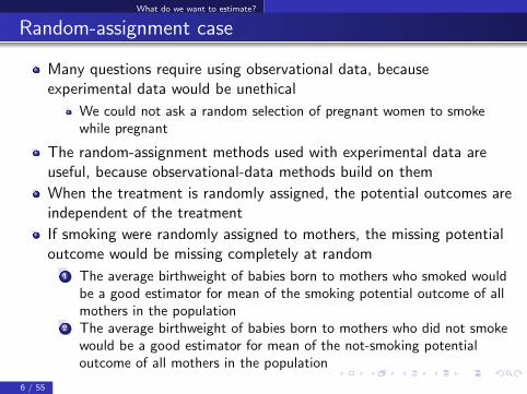
Many questions require using observational data, becauseexperimental data would be unethical
We could not ask a random selection of pregnant women to smokewhile pregnant
The random-assignment methods used with experimental data areuseful, because observational-data methods build on them
When the treatment is randomly assigned, the potential outcomes areindependent of the treatment
If smoking were randomly assigned to mothers, the missing potentialoutcome would be missing completely at random
1 The average birthweight of babies born to mothers who smoked wouldbe a good estimator for mean of the smoking potential outcome of allmothers in the population
2 The average birthweight of babies born to mothers who did not smokewould be a good estimator for mean of the not-smoking potentialoutcome of all mothers in the population
6 / 55
What do we want to estimate?
As good as random
Instead of assuming that the treatment is randomly assigned, weassume that the treatment is as good as randomly assigned afterconditioning on covariates
Formally, this assumption is known as conditional independence
Even more formally, we only need conditional mean independencewhich says that after conditioning on covariates, the treatment doesnot affect the means of the potential outcomes
7 / 55

What do we want to estimate?
Assumptions used with observational data
The assumptions we need vary over estimator and effect parameter,but some version of the following assumptions are required for theexogenous treatment estimators discussed here
CMI The conditional mean-independence CMI assumption restricts thedependence between the treatment model and the potential outcomes
Overlap The overlap assumption ensures that each individual could get anytreatment level
IID The independent-and-identically-distributed (IID) sampling assumptionensures that the potential outcomes and treatment status of eachindividual are unrelated to the potential outcomes and treatmentstatuses of all the other individuals in the population
Endogenous treatment effect models replace CMI with a weakerassumption
In practice, we assume independent observations, not IID
8 / 55

What do we want to estimate?
Some references for assumptions
For Reference Only
Versions of the CMI assumption are also known as unconfoundednessand selection-on-observables in the literature; see Rosenbaum andRubin (1983), Heckman (1997), Heckman and Navarro-Lozano(2004), (Cameron and Trivedi, 2005, section 25.2.1), (Tsiatis, 2006,section 13.3), (Angrist and Pischke, 2009, chapter 3), Imbens andWooldridge (2009), and (Wooldridge, 2010, section 21.3)
Rosenbaum and Rubin (1983) call the combination of conditionalindependence and overlap assumptions strong ignorability; see also(Abadie and Imbens, 2006, pp 237-238) and Imbens and Wooldridge(2009).
The IID assumption is a part of what is known as the stable unittreatment value assumption (SUTVA); see (Wooldridge, 2010, p.905)and Imbens and Wooldridge (2009)
9 / 55
Estimators: Overview
Choice of auxiliary model
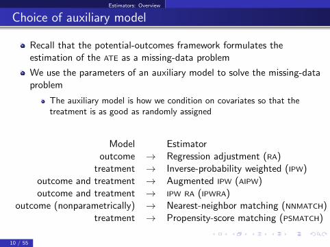
Recall that the potential-outcomes framework formulates theestimation of the ATE as a missing-data problem
We use the parameters of an auxiliary model to solve the missing-dataproblem
The auxiliary model is how we condition on covariates so that thetreatment is as good as randomly assigned
Model Estimatoroutcome → Regression adjustment (RA)
treatment → Inverse-probability weighted (IPW)outcome and treatment → Augmented IPW (AIPW)outcome and treatment → IPW RA (IPWRA)
outcome (nonparametrically) → Nearest-neighbor matching (NNMATCH)treatment → Propensity-score matching (PSMATCH)
10 / 55
Estimators: RA
Regression adjustment estimators
Regression adjustment (RA) estimators:
RA estimators run separate regressions for each treatment level, then
means of predicted outcomes using all the data and the estimatedcoefficients for treatment level i all the data estimate POMi
use differences of POMs, or conditional on the treated POMs, toestimate ATEs or ATETs
Formally, the CMI assumption implies that our regressions of observed yfor a given treatment level directly estimate E[yt |xi ]
yt is the potential outcome for treatment level txi are the covariates on which we conditionAverages of predicted E[yt |xi ] yield estimates of the POM E[yt ] because
1/N∑N
i=1 E[yt |xi ] →p Ex [E[yt |xi ]] = E[yt ]
See (Cameron and Trivedi, 2005, chapter 25), (Wooldridge, 2010,chapter 21), and (Vittinghoff et al., 2012, chapter 9)
11 / 55
Estimators: RA
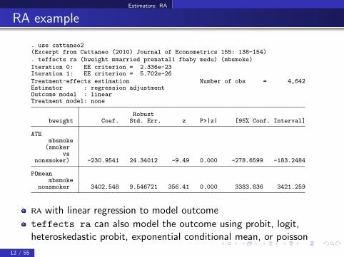
RA example
. use cattaneo2(Excerpt from Cattaneo (2010) Journal of Econometrics 155: 138-154). teffects ra (bweight mmarried prenatal1 fbaby medu) (mbsmoke)Iteration 0: EE criterion = 2.336e-23Iteration 1: EE criterion = 5.702e-26Treatment-effects estimation Number of obs = 4,642Estimator : regression adjustmentOutcome model : linearTreatment model: none
Robustbweight Coef. Std. Err. z P>|z| [95% Conf. Interval]
ATEmbsmoke(smoker
vsnonsmoker) -230.9541 24.34012 -9.49 0.000 -278.6599 -183.2484
POmeanmbsmoke
nonsmoker 3402.548 9.546721 356.41 0.000 3383.836 3421.259
RA with linear regression to model outcome
teffects ra can also model the outcome using probit, logit,heteroskedastic probit, exponential conditional mean, or poisson
12 / 55

Estimators: RA
Why are the standard errors always robust?
have a multistep estimator1 Regress y on x for not treated observations2 Regress y on x for treated observations3 Mean of all observations of predicted y given x from not-treated
regression estimates4 Mean of all observations of predicted y given x from treated regression
estimates
Each step can be obtained by solving moment conditions yielding amethod of moments estimator known as an estimating equation (EE)estimator
mi (θ) is vector of moment equations and m(θ) = 1/N∑N
i=1 mi (θ)
The estimator for the variance-covariance matrix of the estimator has
the form 1/N(DMD ′) where D =(
1N
∂m(θ)∂θ
)−1and
M = 1N
∑Ni=1 mi (θ)mi (θ)
Stacked moments do not yield a symmetric D, so no simplificationunder correct specification
13 / 55

Estimators: IPW
Inverse-probability-weighted estimators
Inverse-probability-weighted (IPW) estimators:
IPW estimators weight observations on the outcome variable by theinverse of the probability that it is observed to account for themissingness processObservations that are not likely to contain missing data get a weightclose to one; observations that are likely to contain missing data get aweight larger than one, potentially much largerIPW estimators model the probability of treatment without anyassumptions about the functional form for the outcome modelIn contrast, RA estimators model the outcome without any assumptionsabout the functional form for the probability of treatment model
See Horvitz and Thompson (1952) Robins and Rotnitzky (1995),Robins et al. (1994), Robins et al. (1995), Imbens (2000), Wooldridge(2002), Hirano et al. (2003), (Tsiatis, 2006, chapter 6), Wooldridge(2007) and (Wooldridge, 2010, chapters 19 and 21)
14 / 55

Estimators: IPW
. teffects ipw (bweight ) (mbsmoke mmarried prenatal1 fbaby medu)Iteration 0: EE criterion = 1.701e-23Iteration 1: EE criterion = 6.339e-27Treatment-effects estimation Number of obs = 4,642Estimator : inverse-probability weightsOutcome model : weighted meanTreatment model: logit
Robustbweight Coef. Std. Err. z P>|z| [95% Conf. Interval]
ATEmbsmoke(smoker
vsnonsmoker) -231.1516 24.03183 -9.62 0.000 -278.2531 -184.0501
POmeanmbsmoke
nonsmoker 3402.219 9.589812 354.77 0.000 3383.423 3421.015
IPW with logit to model treatment
Could have used probit or heteroskedastic probit to model treatment
Estimator has stacked moment structure; score equations fromfirst-stage maximum-likelihood estimators are now moment equations
15 / 55

Checking for balance
Balance: As good as random
In the unobtainable case of a randomly assigned treatment, thedistribution of the covariates among those that get the treatment isthe same as the distribution of the covariates among those that donot get the treatment
The distribution of the covariates is said to be “balanced” over thetreatment/control status
The estimators implemented in teffects use a model or matchingmethod to make the outcome conditionally independent of thetreatment by conditioning on covariates
If this model or matching method is well specified, it should balancethe covariatesBalance diagnostic techniques and tests check the specification of theconditioning method used by a teffects
16 / 55

Checking for balance
Balance with IPW
Rosenbaum and Rubin (1983) showed that the propensity score is abalancing score
In particular, the treatment is conditionally independent of thecovariates after conditioning on the propensity scoreAmong the many applications of this result is the implication that IPW
means of covariates will be the same for treated and controlsThe raw means of covariates will differ over treated and controlobservations, but the IPW means will be similar
17 / 55

Checking for balance
tebalance
tebalance implements diagnostics and a test for balance afterteffects
Diagnostics are statistics and graphical methods for which we do notknow the distribution under the nullA test is a statistic for which we know the distribution under the null
tebalance is new to Stata 14
18 / 55

Checking for balance
An example using the Cattaneo data
Let’s look for evidence against balancing using the simple model
. clear all
. use cattaneo2(Excerpt from Cattaneo (2010) Journal of Econometrics 155: 138-154). quietly teffects ipw (bweight) (mbsmoke mmarried mage prenatal1 fbaby medu)>. tebalance summarizeCovariate balance summary
Raw Weighted
Number of obs = 4,642 4,642.0Treated obs = 864 2,280.4Control obs = 3,778 2,361.6
Standardized differences Variance ratioRaw Weighted Raw Weighted
mmarried -.5953009 -.0258113 1.335944 1.021696mage -.300179 -.0803657 .8818025 .8127244
prenatal1 -.3242695 -.0228922 1.496155 1.034023fbaby -.1663271 .0221042 .9430944 1.005032medu -.5474357 -.1373455 .7315846 .4984786
19 / 55

Checking for balance
Standardized differences
Group differences scaled by the average the group variances areknown as known as standardized differences
The raw standardized differences between treatment levels t1 and t0
are
δ(t1, t0) =µx(t1)− µx(t1)√σ2x(t1) + σ2
x(t0)
where
µx(t) =1
Nt
N∑i=1
(ti == t)xi
σx(t) =1
Nt − 1
N∑i=1
(ti == t) (xi − µx(t))2
20 / 55

Checking for balance
IPW standardized differences
If the model for the treatment is correctly specified, the IPWstandardized differences will be zero
The IPW standardized differences between treatment levels t1 and t0
are
δ(t1, t0) =µx(t1)− µx(t1)√σ2x(t1) + σ2
x(t0)
where
µx(t) =1
Mt
N∑i=1
ωi (ti == t)xi
σx(t) =1
Mt − 1
N∑i=1
(ti == t)ωi (xi − µx(t))2
and ωi are the normalized predicted treatment probabilities andMt =
∑Ni=1(t1 == t)ωi
21 / 55

Checking for balance
Test for balance
Imai and Ratkovic (2014) derived a test for balance by viewing therestrictions imposed by balance as overidentifying conditions.
Scores for ML estimator of propensity score are moment conditionsMoment conditions for equality of means are over-identifing conditionsEstimate over-identified parameters by generalized method of moments(GMM)Under the null of covariate balance GMM criterion statistic has χ2(J)distribution, where J is the number of over-identifying momentconditions imposed by covariate balance
22 / 55

Checking for balance
. quietly teffects ipw (bweight) (mbsmoke mmarried mage prenatal1 fbaby medu)>. tebalance overidIteration 0: criterion = .01513068Iteration 1: criterion = .01514951 (backed up)Iteration 2: criterion = .01521006Iteration 3: criterion = .01539644Iteration 4: criterion = .01542377Iteration 5: criterion = .01550797Iteration 6: criterion = .01553409Iteration 7: criterion = .01558562Iteration 8: criterion = .01568553Iteration 9: criterion = .01569183Iteration 10: criterion = .01572721Iteration 11: criterion = .01573403Iteration 12: criterion = .01573406Overidentification test for covariate balance
H0: Covariates are balanced:chi2(6) = 62.5564Prob > chi2 = 0.0000
Reject null hypothesis that IPW model/weights balance covariates
23 / 55

Model selection
Model selection
How to selection the model for the outcome or the treatment?
Use theory to decide the set of covariates
Do not condition on variables that are affected by the treatment,Wooldridge (2005)
What functional form of a set or super set of the correct covariatesshould I use?
24 / 55

Model selection
Minimizing an information criterion
The idea is to fit a bunch of models and select the model withsmallest information criterion
An information criterion is -LL + penalty term
The better the estimator fits the data, the smaller is the negative ofthe log-likelihood (-LL)The more parameters are added to the model, the larger is the penaltyterm
Choosing the model that minimizes an information criteria has a longhistory in statistics and econometrics
Claeskens and Hjort (2008), (Cameron and Trivedi, 2005, Section8.5.1)
25 / 55
Model selection
Minimizing an information criterion
Minimizing the Bayesian information criterion (BIC) can be aconsistent model selection technique
Selecting the model that minimizes the BIC is an estimator of whichmodel to selectThe model selected by this estimator converges to the true model asthe sample size gets largerBIC = −2LL + 2 ln(N)q, where N is the sample size and q is thenumber of parameters
Minimizing the Akaike information criterion (AIC) tends to select amodel with too many terms
The model selected by this estimator converges to a model that overfits as the sample size gets largerAIC = −2LL + 2q
26 / 55

Model selection
bfit does model selection
bfit is a user written command documented in Cattaneo et al.(2013)
bfit will find the model that minimizes either the BIC or the AIC
within a subset of all possible models
27 / 55

Model selection
. bfit logit mbsmoke mmarried mage prenatal1 fbaby medubfit logit results sorted by bic
Model Obs ll(null) ll(model) df AIC BIC
_bfit_32 4642 -2230.748 -2002.985 9 4023.97 4081.956_bfit_30 4642 -2230.748 -2012.263 7 4038.525 4083.626_bfit_31 4642 -2230.748 -2008.151 8 4032.302 4083.845_bfit_33 4642 -2230.748 -1995.658 12 4015.316 4092.631_bfit_34 4642 -2230.748 -1989.613 18 4015.225 4131.197_bfit_19 4642 -2230.748 -2033.762 8 4083.524 4135.067_bfit_18 4642 -2230.748 -2040.745 7 4095.49 4140.591_bfit_25 4642 -2230.748 -2039.028 8 4094.056 4145.6_bfit_16 4642 -2230.748 -2053.041 5 4116.081 4148.296_bfit_17 4642 -2230.748 -2049.147 6 4110.294 4148.952_bfit_26 4642 -2230.748 -2033.566 10 4087.132 4151.561_bfit_12 4642 -2230.748 -2051.069 6 4114.138 4152.796_bfit_23 4642 -2230.748 -2051.658 6 4115.316 4153.974_bfit_24 4642 -2230.748 -2047.907 7 4109.815 4154.915_bfit_20 4642 -2230.748 -2027.135 12 4078.271 4155.585_bfit_14 4642 -2230.748 -2029.388 12 4082.776 4160.091_bfit_11 4642 -2230.748 -2055.651 6 4123.303 4161.96_bfit_13 4642 -2230.748 -2044.248 9 4106.496 4164.482_bfit_35 4642 -2230.748 -1983.735 24 4015.469 4170.099_bfit_21 4642 -2230.748 -2017.789 16 4067.577 4170.664_bfit_9 4642 -2230.748 -2072.867 4 4153.733 4179.505_bfit_27 4642 -2230.748 -2026.593 15 4083.186 4179.83_bfit_10 4642 -2230.748 -2069.425 5 4148.85 4181.065_bfit_7 4642 -2230.748 -2060.093 8 4136.187 4187.73_bfit_28 4642 -2230.748 -2016.621 20 4073.242 4202.1_bfit_4 4642 -2230.748 -2082.388 5 4174.776 4206.99_bfit_6 4642 -2230.748 -2079.501 6 4171.003 4209.66_bfit_5 4642 -2230.748 -2088.62 4 4185.241 4211.012_bfit_29 4642 -2230.748 -2085.159 6 4182.317 4220.975_bfit_3 4642 -2230.748 -2102.649 4 4213.297 4239.069_bfit_2 4642 -2230.748 -2109.805 3 4225.61 4244.939_bfit_15 4642 -2230.748 -2133.02 4 4274.041 4299.812_bfit_22 4642 -2230.748 -2130.327 5 4270.653 4302.868_bfit_8 4642 -2230.748 -2138.799 3 4283.598 4302.926_bfit_1 4642 -2230.748 -2200.161 2 4404.322 4417.207
Note: N= used in calculating BIC(results _bfit_32 are active now). display "`r(bvlist)´"i.(mmarried prenatal1 fbaby) mage medu c.mage#c.mage c.mage#c.medu c.medu#c.med> u
28 / 55

Model selection
Over-identification test with selected model
. teffects ipw (bweight) (mbsmoke i.(mmarried prenatal1 fbaby) mage medu ///> c.mage#c.mage c.mage#c.medu c.medu#c.medu), nologTreatment-effects estimation Number of obs = 4,642Estimator : inverse-probability weightsOutcome model : weighted meanTreatment model: logit
Robustbweight Coef. Std. Err. z P>|z| [95% Conf. Interval]
ATEmbsmoke(smoker
vsnonsmoker) -220.7592 28.47705 -7.75 0.000 -276.5732 -164.9452
POmeanmbsmoke
nonsmoker 3403.625 9.544666 356.60 0.000 3384.917 3422.332
. tebalance overid, nologOveridentification test for covariate balance
H0: Covariates are balanced:chi2(9) = 9.38347Prob > chi2 = 0.4027
29 / 55

Survival-time data
Survival-time example
Does smoking decrease the time to a second heart attack in thepopulation of women aged 45–55 who have had one heart attack?
1 For ethical reasons, these data will be observational.
2 This question is about the time to an event, and such data arecommonly known as survival-time data or time-to-event data. Thesedata are nonnegative and, frequently, right-censored.
3 Many researchers and practitioners want an effect estimate ineasy-to-understand units of time.
30 / 55

Survival-time data
Much of the survival-time literature uses a hazard ratio as the effect ofinterest. The ATE has three advantages over the hazard ratio as an effectmeasure.
1 The ATE measures the effect in the same time units as the outcomeinstead of in relative conditional probabilities.
2 The ATE is much easier to explain to nontechnical audiences.
3 The models used to estimate the ATE can be much more flexible.
Hazard ratios are useful for population effects when they are constant,which occurs when the treatment enters linearly and the distributionof the outcome has a proportional-hazards form.
Neither linearity in treatment nor proportional-hazards form isrequired for the ATE, and neither is imposed on the models fit by theestimators implemented in stteffects.
31 / 55

Survival-time data
Estimators in stteffectsRegression adjustment (RA)
Model outcomeTreatment assignment is handled by estimating seperate models foreach treatment levelCensoring handled in log-likelihood function for outcome
Inverse-probability weighting
Model treatment assignmentOutcome is not modeled; estimated is weighted average of observedoutcomesCensoring handled my modeling time to censoring, which must berandom
Inverse-probability weighted regression adjustment (IPWRA)
Model outcome and treatmentCensoring handled in one of two ways
Censoring handled in log-likelihood function for outcome, orCensoring handled my modeling time to censoring, which must berandom
stteffects is new Stata 1432 / 55
Survival-time data
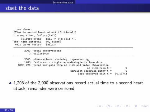
stset the data
. use sheart(Time to second heart attack (fictional)). stset atime, failure(fail)
failure event: fail != 0 & fail < .obs. time interval: (0, atime]exit on or before: failure
2000 total observations0 exclusions
2000 observations remaining, representing1208 failures in single-record/single-failure data
3795.226 total analysis time at risk and under observationat risk from t = 0
earliest observed entry t = 0last observed exit t = 34.17743
1,208 of the 2,000 observations record actual time to a second heartattack; remainder were censored
33 / 55

Survival-time data
stteffects ra
. stteffects ra (age exercise diet education) (smoke)failure _d: fail
analysis time _t: atimeIteration 0: EE criterion = 1.525e-19Iteration 1: EE criterion = 2.965e-30Survival treatment-effects estimation Number of obs = 2,000Estimator : regression adjustmentOutcome model : WeibullTreatment model: noneCensoring model: none
Robust_t Coef. Std. Err. z P>|z| [95% Conf. Interval]
ATEsmoke
(Smokervs
Nonsmoker) -1.956657 .3331787 -5.87 0.000 -2.609676 -1.303639
POmeansmoke
Nonsmoker 4.243974 .2620538 16.20 0.000 3.730358 4.75759
34 / 55
Survival-time data
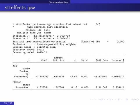
stteffects ipw
. stteffects ipw (smoke age exercise diet education) ///> (age exercise diet education)
failure _d: failanalysis time _t: atime
Iteration 0: EE criterion = 2.042e-18Iteration 1: EE criterion = 1.008e-31Survival treatment-effects estimation Number of obs = 2,000Estimator : inverse-probability weightsOutcome model : weighted meanTreatment model: logitCensoring model: Weibull
Robust_t Coef. Std. Err. z P>|z| [95% Conf. Interval]
ATEsmoke
(Smokervs
Nonsmoker) -2.187297 .6319837 -3.46 0.001 -3.425962 -.9486314
POmeansmoke
Nonsmoker 4.225331 .517501 8.16 0.000 3.211047 5.239614
35 / 55

Survival-time data
stteffects ipwra: likelihood adjustment for censoring
. stteffects ipwra (age exercise diet education) ///> (smoke age exercise diet education)
failure _d: failanalysis time _t: atime
Iteration 0: EE criterion = 2.153e-16Iteration 1: EE criterion = 6.312e-30Survival treatment-effects estimation Number of obs = 2,000Estimator : IPW regression adjustmentOutcome model : WeibullTreatment model: logitCensoring model: none
Robust_t Coef. Std. Err. z P>|z| [95% Conf. Interval]
ATEsmoke
(Smokervs
Nonsmoker) -1.592494 .4872777 -3.27 0.001 -2.54754 -.637447
POmeansmoke
Nonsmoker 4.214523 .2600165 16.21 0.000 3.7049 4.724146
36 / 55

Survival-time data
stteffects ipwra: Weighted adjustment for censoring
. stteffects ipwra (age exercise diet education) ///> (smoke age exercise diet education) ///> (age exercise diet)
failure _d: failanalysis time _t: atime
Iteration 0: EE criterion = 1.632e-16Iteration 1: EE criterion = 4.278e-30Survival treatment-effects estimation Number of obs = 2,000Estimator : IPW regression adjustmentOutcome model : WeibullTreatment model: logitCensoring model: Weibull
Robust_t Coef. Std. Err. z P>|z| [95% Conf. Interval]
ATEsmoke
(Smokervs
Nonsmoker) -2.037944 .6032549 -3.38 0.001 -3.220302 -.855586
POmeansmoke
Nonsmoker 4.14284 .4811052 8.61 0.000 3.199891 5.085789
37 / 55

Endogenous treatment effects
Endogenous treatment effects
Allow an unobserved component to affect treatment assignment andeach potential outcome
Violates CMI even though covariates are unrelated to error terms
View the estimators implemented in eteffects as extentions to RA
for a type of endogenous treatment
eteffects is new to Stata 14
38 / 55

Endogenous treatment effects
Endogenous treatment effects
Here are the equations, when the outcome is linear
y0 = xβ0 + ε0 + γ0ν
y1 = xβ1 + ε1 + γ1ν
t = (zα + ν > 0)
y = ty1 + (1− t)y0
x and z are unrelated to ν and ε
ν ∼ N(0, 1)
The endogeneity is caused by the presence of ν in all the equations
39 / 55

Endogenous treatment effects
Endogenous treatment effects: Method
Estimate probit of treatment on z, and get residuals ν
Regress y on x and ν, when t==0 to get µ0i = E[y0|xi , νi ]Regress y on x and ν, when t==1 to get µ1i = E[y1|xi , νi ]ATE is average of µ1i − µ0i
Correct standard errors by stacking the moment conditions
40 / 55
Endogenous treatment effects
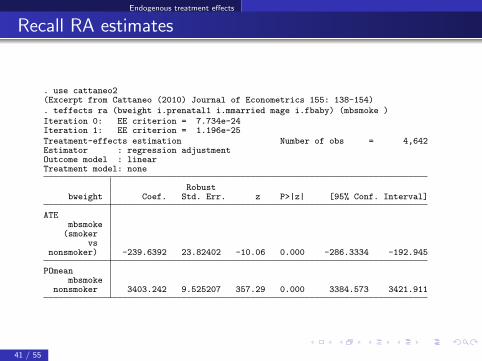
Recall RA estimates
. use cattaneo2(Excerpt from Cattaneo (2010) Journal of Econometrics 155: 138-154). teffects ra (bweight i.prenatal1 i.mmarried mage i.fbaby) (mbsmoke )Iteration 0: EE criterion = 7.734e-24Iteration 1: EE criterion = 1.196e-25Treatment-effects estimation Number of obs = 4,642Estimator : regression adjustmentOutcome model : linearTreatment model: none
Robustbweight Coef. Std. Err. z P>|z| [95% Conf. Interval]
ATEmbsmoke(smoker
vsnonsmoker) -239.6392 23.82402 -10.06 0.000 -286.3334 -192.945
POmeanmbsmoke
nonsmoker 3403.242 9.525207 357.29 0.000 3384.573 3421.911
41 / 55
Endogenous treatment effects
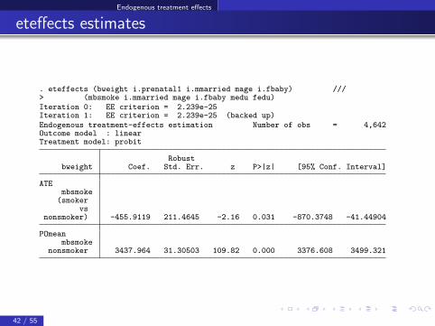
eteffects estimates
. eteffects (bweight i.prenatal1 i.mmarried mage i.fbaby) ///> (mbsmoke i.mmarried mage i.fbaby medu fedu)Iteration 0: EE criterion = 2.239e-25Iteration 1: EE criterion = 2.239e-25 (backed up)Endogenous treatment-effects estimation Number of obs = 4,642Outcome model : linearTreatment model: probit
Robustbweight Coef. Std. Err. z P>|z| [95% Conf. Interval]
ATEmbsmoke(smoker
vsnonsmoker) -455.9119 211.4645 -2.16 0.031 -870.3748 -41.44904
POmeanmbsmoke
nonsmoker 3437.964 31.30503 109.82 0.000 3376.608 3499.321
42 / 55

Endogenous treatment effects
Testing for endogeneity
There is no endogeneity if the coefficients on the control term, thegeneralized residuals, are zero
A Wald test that these coefficients are jointly zero is a test of the nullhypothesis of no endogeneity
43 / 55

Endogenous treatment effects
Testing for endogeneity
. estat endogenousTest of endogeneityHo: treatment and outcome unobservables are uncorrelated
chi2( 2) = 2.12Prob > chi2 = 0.3463
44 / 55

Endogenous treatment effects
Other functional forms
Outcome model in eteffects could be fractional, probit, orexponential-mean, in addition to linear
45 / 55
Endogenous treatment effects
Now what?
Go to http://www.stata.com/manuals14/te.pdf entry teffects
intro advanced for more information and lots of links to literatureand examples
46 / 55

Quantile treatment effects (QTE)
QTEs for survival data
Imagine a study that followed middle-aged men for two years aftersuffering a heart attack
Does exercise affect the time to a second heart attack?Some observations on the time to second heart attack are censoredObservational data implies that treatment allocation depends oncovariatesWe use a model for the outcome to adjust for this dependence
47 / 55

Quantile treatment effects (QTE)
QTEs for survival data
Exercise could help individuals with relatively strong hearts but nothelp those with weak hearts
For each treatment level, a strong-heart individual is in the .75quantile of the marginal, over the covariates, distribution of time tosecond heart attack
QTE(.75) is difference in .75 marginal quantiles
Weak-heart individual would be in the .25 quantile of the marginaldistribution for each treatment level
QTE(.25) is difference in .25 marginal quantiles
our story indicates that the QTE(.75) should be significantly largerthat the QTE(.25)
48 / 55

Quantile treatment effects (QTE)
What are QTEs?
CDF of yexercise →
← CDF of ynoexercise
q Ex(.2
)q NO
Ex(.
2)
q Ex(.8
)
q No E
x(.8)0
.2.4
.6.8
1
Time to second attack
49 / 55

Quantile treatment effects (QTE)
Quantile Treatment effects
We can easily estimate the marginal quantiles, but estimating thequantile of the differences is harder
We need a rank preserveration assumption to ensure that quantile ofthe differences is the difference in the quantiles
The τ(th) quantile of y1 minus the τ(th) quantile of y0 is not the sameas the τ(th) quantile of (y1 − y0) unless we impose a rank-preservationassumptionRank preservation means that the random shocks that affect thetreated and the not-treated potential outcomes do not change the rankof the individuals in the population
The rank of an individual in y1 is the same as the rank of thatindividual in y0
Graphically, the horizontal lines must intersect the CDFs “at the sameindividual”
50 / 55

Quantile treatment effects (QTE)
A regression-adjustment estimator for QTEs
Estimate the θ1 parameters of F (y |x, t = 1,θ1) the CDF conditionalon covariates and conditional on treatment level
Conditional independence implies that this conditional on treatmentlevel CDF estimates the CDF of the treated potential outcome
Similarly, estimate the θ0 parameters of F (y |x, t = 0,θ0)
At the point y ,
1/NN∑i=1
F (y |xi , θ1)
estimates the marginal distribution of the treated potential outcome
The q1,.75 that solves
1/NN∑i=1
F (q1,.75|xi , θ1) = .75
estimates the .75 marginal quantile for the treated potential outcome
51 / 55
Quantile treatment effects (QTE)
A regression-adjustment estimator for QTEs
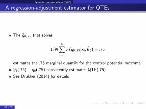
The q0,.75 that solves
1/NN∑i=1
F (q0,.75|xi , θ0) = .75
estimates the .75 marginal quantile for the control potential outcome
q1(.75)− q0(.75) consistently estimates QTE(.75)
See Drukker (2014) for details
52 / 55

Quantile treatment effects (QTE)
mqgamma example
mqgamma is a user-written command documented in Drukker (2014)
. ssc install mqgamma
. use exercise, clear
. mqgamma t active, treat(exercise) fail(fail) lns(health) quantile(.25 .75)Iteration 0: EE criterion = .7032254Iteration 1: EE criterion = .05262105Iteration 2: EE criterion = .00028553Iteration 3: EE criterion = 6.892e-07Iteration 4: EE criterion = 4.706e-12Iteration 5: EE criterion = 1.604e-22Gamma marginal quantile estimation Number of obs = 2000
Robustt Coef. Std. Err. z P>|z| [95% Conf. Interval]
q25_0_cons .2151604 .0159611 13.48 0.000 .1838771 .2464436
q25_1_cons .2612655 .0249856 10.46 0.000 .2122946 .3102364
q75_0_cons 1.591147 .0725607 21.93 0.000 1.44893 1.733363
q75_1_cons 2.510068 .1349917 18.59 0.000 2.245489 2.774647
53 / 55
Quantile treatment effects (QTE)
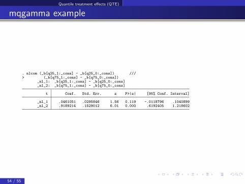
mqgamma example
. nlcom (_b[q25_1:_cons] - _b[q25_0:_cons]) ///> (_b[q75_1:_cons] - _b[q75_0:_cons])
_nl_1: _b[q25_1:_cons] - _b[q25_0:_cons]_nl_2: _b[q75_1:_cons] - _b[q75_0:_cons]
t Coef. Std. Err. z P>|z| [95% Conf. Interval]
_nl_1 .0461051 .0295846 1.56 0.119 -.0118796 .1040899_nl_2 .9189214 .1529012 6.01 0.000 .6192405 1.218602
54 / 55
Quantile treatment effects (QTE)
poparms also estimates QTEs
poparms is a user-written command documented in Cattaneo,Drukker, and Holland (2013)
poparms estimates mean and quantiles of the potential-outcomedistributions
poparms implements an IPW and an AIPW derived in Cattaneo (2010)Cattaneo (2010) and Cattaneo, Drukker, and Holland (2013) call theAIPW estimator an efficient-influence function (EIF) estimator becauseEIF theory is what produces the augmentation term
55 / 55

References
Abadie, Alberto and Guido W. Imbens. 2006. “Large sample properties ofmatching estimators for average treatment effects,” Econometrica,235–267.
Angrist, J. D. and J.-S. Pischke. 2009. Mostly Harmless Econometrics: AnEmpiricist’s Companion, Princeton, NJ: Princeton University Press.
Cameron, A. Colin and Pravin K. Trivedi. 2005. Microeconometrics:Methods and applications, Cambridge: Cambridge University Press.
Cattaneo, Matias D., David M. Drukker, and Ashley D. Holland. 2013.“Estimation of multivalued treatment effects under conditionalindependence,” Stata Journal, 13(3), 407–450.
Cattaneo, M.D. 2010. “Efficient semiparametric estimation of multi-valuedtreatment effects under ignorability,” Journal of Econometrics, 155(2),138–154.
Claeskens, Gerda and Nils Lid Hjort. 2008. Model selection and modelaveraging, Cambridge, UK: Cambridge University Press.
Drukker, David M. 2014. “Quantile treatment effect estimation fromcensored data by regression adjustment,” Tech. rep., Under review atthe Stata Journal, http://www.stata.com/ddrukker/mqgamma.pdf.
55 / 55

References
Heckman, James and Salvador Navarro-Lozano. 2004. “Using matching,instrumental variables, and control functions to estimate economicchoice models,” Review of Economics and statistics, 86(1), 30–57.
Heckman, James J. 1997. “Instrumental variables: A study of implicitbehavioral assumptions used in making program evaluations,” Journal ofHuman Resources, 32(3), 441–462.
Hirano, Keisuke, Guido W. Imbens, and Geert Ridder. 2003. “Efficientestimation of average treatment effects using the estimated propensityscore,” Econometrica, 71(4), 1161–1189.
Holland, Paul W. 1986. “Statistics and causal inference,” Journal of theAmerican Statistical Association, 945–960.
Horvitz, D. G. and D. J. Thompson. 1952. “A Generalization of SamplingWithout Replacement From a Finite Universe,” Journal of the AmericanStatistical Association, 47(260), 663–685.
Imai, Kosuke and Marc Ratkovic. 2014. “Covariate balancing andpropensity score,” Journal of the Royal Statistical Society: Series B,76(1), 243–263.
55 / 55

References
Imbens, Guido W. 2000. “The role of the propensity score in estimatingdose-response functions,” Biometrika, 87(3), 706–710.
———. 2004. “Nonparametric estimation of average treatment effectsunder exogeneity: A review,” Review of Economics and statistics, 86(1),4–29.
Imbens, Guido W. and Jeffrey M. Wooldridge. 2009. “RecentDevelopments in the Econometrics of Program Evaluation,” Journal ofEconomic Literature, 47, 5–86.
Robins, James M. and Andrea Rotnitzky. 1995. “Semiparametric Efficiencyin Multivariate Regression Models with Missing Data,” Journal of theAmerican Statistical Association, 90(429), 122–129.
Robins, James M., Andrea Rotnitzky, and Lue Ping Zhao. 1994.“Estimation of Regression Coefficients When Some Regressors Are NotAlways Observed,” Journal of the American Statistical Association,89(427), 846–866.
———. 1995. “Analysis of Semiparametric Regression Models forRepeated Outcomes in the Presence of Missing Data,” Journal of theAmerican Statistical Association, 90(429), 106–121.
55 / 55

References
Rosenbaum, P. and D. Rubin. 1983. “Central Role of the Propensity Scorein Observational Studies for Causal Effects,” Biometrika, 70, 41–55.
Rubin, Donald B. 1974. “Estimating causal effects of treatments inrandomized and nonrandomized studies.” Journal of educationalPsychology, 66(5), 688.
Tsiatis, Anastasios A. 2006. Semiparametric theory and missing data, NewYork: Springer Verlag.
Vittinghoff, E., D. V. Glidden, S. C. Shiboski, and C. E. McCulloch. 2012.Regression Methods in Biostatistics: Linear, Logistic, Survival, andRepeated Measures Models, New York: Springer, 2 ed.
Wooldridge, Jeffrey M. 2002. “Inverse probability weighted M-estimatorsfor sample selection, attrition, and stratification,” Portuguese EconomicJournal, 1, 117–139.
Wooldridge, Jeffrey M. 2005. “Violating ignorability of treatment bycontrolling for too many factors,” Econometric Theory, 21(5), 1026.
Wooldridge, Jeffrey M. 2007. “Inverse probability weighted estimation forgeneral missing data problems,” Journal of Econometrics, 141(2),1281–1301.
55 / 55

Bibliography
———. 2010. Econometric Analysis of Cross Section and Panel Data,Cambridge, Massachusetts: MIT Press, second ed.
55 / 55