estimating trends in the global mean temperature … trends in the global mean temperature record...
TRANSCRIPT

Estimating trends in the global mean temperature
record
Andrew Poppick∗
Department of Mathematics and Statistics, Carleton College,Elisabeth J. Moyer
Department of the Geophysical Sciences, University of Chicagoand
Michael L. SteinDepartment of Statistics, University of Chicago
May 8, 2018
Abstract
Physical models suggest that the Earth’s mean temperature warms in response tochanging CO2 concentrations (and hence increased radiative forcing); given physicaluncertainties in this relationship, the historical temperature record is a source of em-pirical information about global warming. A persistent thread in many analyses of thehistorical temperature record, however, is the reliance on methods that appear to deem-phasize both physical and statistical assumptions. Examples include regression modelsthat treat time rather than radiative forcing as the relevant covariate, and time seriesmethods that account for natural variability in nonparametric rather than parametricways. We show here that methods that deemphasize assumptions can limit the scopeof analysis and can lead to misleading inferences, particularly in the setting consideredwhere the data record is relatively short and the scale of temporal correlation is rela-tively long. A proposed model that is simple but physically informed provides a morereliable estimate of trends and allows a broader array of questions to be addressed. Inaccounting for uncertainty, we also illustrate how parametric statistical models thatare attuned to the important characteristics of natural variability can be more reliablethan ostensibly more flexible approaches.
Keywords: Climate change; climate sensitivity; time series; parametric modeling; bootstrap.
∗The authors thank Jonah Bloch-Johnson, Malte Jansen, Cristian Proistosescu, and Kate Marvel forhelpful conversations and comments related to parts of this work. This work was supported in part bySTATMOS, the Research Network for Statistical Methods for Atmospheric and Oceanic Sciences (NSF-DMS awards 1106862, 1106974 and 1107046), and RDCEP, the University of Chicago Center for RobustDecision Making in Climate and Energy Policy (NSF Grant SES-0951576). We thank NASA GISS, NOAA,the Hadley Centre, the IPCC, and IIASA for the use of their publicly available data. We acknowledge theUniversity of Chicago Research Computing Center, whose resources were used in the completion of thiswork.
1
arX
iv:1
607.
0385
5v1
[st
at.A
P] 1
3 Ju
l 201
6

1 Introduction
The physical basis of climate change is understood through a combination of physical theory,numerical simulations, and analyses of historical data. A fundamental concept to explainglobal warming is that of radiative forcing, which is the change in net radiation (down-welling minus upwelling, typically expressed in units of W/m2, at the top of atmosphere)resulting from an imposed perturbation of a climate in equilibrium, such as a change inthe atmospheric concentration of a greenhouse gas. An increase in atmospheric CO2, forexample, reduces upwelling radiation and produces a net influx of heat; the Earth’s surfacethen warms until radiative equilibrium is restored. The most important source of forcing inthe present climate is anthropogenic emissions of CO2, but other anthropogenic or naturalforcing agents also contribute to climate change. (Anthropogenic agents include more mi-nor greenhouse gases and aerosols; natural agents include aerosols from volcanic eruptionsand periodic variations in solar insolation.) The Earth’s response to forcing is complexand not fully understood, as there are physical uncertainties in important feedbacks suchas cloud responses. A comprehensive source of information about climate change can befound in the assessment reports of the Intergovernmental Panel on Climate Change (IPCC)(the most recent being IPCC (2013)).
Given these physical uncertainties, the observed global mean temperature record sincethe late nineteenth century is a source of empirical information about the Earth’s system-atic response to forcing. (Figure 1 shows one estimate of annually averaged global meansurface temperatures from the past 136 years along with estimates of radiative forcingsfrom various constituents during that period, with the data sources described in Section 2.)Analysis of the observed temperature record is complicated by the short available record ofdirect measurements, by uncertainties in the historical radiative forcings themselves, andby the natural temperature variability that exists even in the absence of forcing. Statisticalmethods are required to quantify the information in the historical record about the responseto forcing: given the data, what do we know about how global temperatures have warmedin response to forcing, how much warming can we expect in plausible future forcing scenar-ios, and how do we expect uncertainties to change as we continue to observe the Earth’stemperatures?
One common approach to using the observed temperature record to understand aspectsof climate change is to assume a physical model of the system. Such a model can range froma simple energy balance model to a very complicated atmosphere-ocean general circulationmodel (GCM). Examples of analyses of observed temperatures using simple or moderatelycomplex physical models to estimate expected changes due to forcing include Gregory et al.(2002), Forest et al. (2006), Gregory and Forster (2008), Padilla et al. (2011), Aldrin et al.(2012), Otto et al. (2013), Masters (2014), Lewis and Curry (2015), and many others; seealso IPCC (2013) Chapter 10 and references therein for methods using GCMs.
Other approaches are more empirical and appear to deemphasize assumptions aboutthe underlying physics generating the observed temperatures. These ostensibly objectiveanalyses can involve both parts of the statistical modeling endeavor, i.e., characterizingboth the systematic response and the natural variability. First, in modeling the systematicresponse of temperatures over time, it is somewhat common practice to use regression mod-els that treat time rather than radiative forcing as the covariate. Studies that incorporatethis practice into analyses testing for either significant warming or changes in warmingtrends include Bloomfield (1992), Smith and Chen (1996), Foster and Rahmstorf (2011),
2

Year
Tem
pera
ture
Ano
mal
y (°
C)
1880 1910 1940 1970 2000
−0.
4−
0.2
0.0
0.2
0.4
0.6
0.8
Year
Rad
iativ
e F
orci
ng (
W/m
2 )
CO2
Other GHGAerosols (tropospheric)SolarVolcanosOther
Net ForcingNet Anthropogenic Forcing
1880 1910 1940 1970 2000
−3
−2
−1
01
2
●
●●
●
●
● ●●
●
●
●
●●
● ●
●
●
●
●
●
●
●
●
●
●
●
●
●●
●
●●
●●
●
●
●
●
●●
●
●
●●
●
●
●
●●
●
●
●
●
●
●
●
●
●●●
●
●●
●
●
●
● ●
●●
●
●
●
●
●●
●
●●
●
●
●●
●
●
●
●●
●
●●
●
●
●
●
●
●
●
●
●
●
●
●
●
●
●
●
●
●
●
●●
● ●
●
●
●
●
●
●●
●
●●
●
●
●●
●
●
●
●●
●
●
●
Net Radiative Forcing (W/m2)Tem
pera
ture
Ano
mal
y (°
C)
−3 −2 −1 0 1 2
−0.
40.
00.
40.
8
●
●●
●
●
●●●
●
●
●
●●●●
●
●
●
●
●
●
●
●
●
●
●
●
●●
●
●●
●●
●
●
●
●
●●●
●
●●
●
●
●
●●
●
●
●
●
●
●
●
●
●●●
●
●●
●
●
●
●●
●●
●
●
●
●
●●
●
●●●
●
●●
●
●
●
●●
●
●●
●
●
●
●
●
●
●
●
●
●
●
●
●
●
●
●
●
●
●
●●
●●
●
●
●
●
●
●●
●
●●
●
●
●●
●
●
●
●●
●
●
●
Anthropogenic Forcing (W/m2)Tem
pera
ture
Ano
mal
y (°
C)
−3 −2 −1 0 1 2
−0.
40.
00.
40.
8
●
●●
●
●
● ●●
●
●
●
●●
● ●
●
●
●
●
●
●
●
●
●
●
●
●
●●
●
●●
●●
●
●
●
●
●●
●
●
●●
●
●
●
●●
●
●
●
●
●
●
●
●
●●●
●
●●
●
●
●
● ●
●●
●
●
●
●
●●
●
●●
●
●
●●
●
●
●
●●
●
●●
●
●
●
●
●
●
●
●
●
●
●
●
●
●
●
●
●
●
●
●●
● ●
●
●
●
●
●
●●
●
●●
●
●
●●
●
●
●
●●●
●
●
Natural Forcing (W/m2)Tem
pera
ture
Ano
mal
y (°
C)
−3 −2 −1 0 1 2
−0.
40.
00.
40.
8
Figure 1: Top left, estimates of annually averaged global mean surface temperature anoma-lies (relative to a base period of 1951-1980) from the years 1880 to 2015. Bottom left,estimates of (top-of-atmosphere) effective radiative forcings from different constituents overthis time period (the “other” category includes O3, H2O, black carbon, contrails, and landuse changes). Right, temperature anomalies vs. net radiative forcings (top), vs. anthro-pogenic forcing (middle), and vs. natural forcing (bottom). Data sources are described inSection 2. Despite the plots of temperature vs. radiative forcing, temperatures will dependon the full past trajectory of radiative forcings in a potentially complex way, as we discussin Section 3.
3

Cahill et al. (2015), Rajaratnam et al. (2015), and Løvsletten and Rypdal (2016), andmany others. (See also IPCC (2013), especially Chapter 2 Box 2.2, and references therein.)Second, in coping with natural variability for the purpose of uncertainty quantification,some authors prefer nonparametric (resampling or subsampling) methods for time seriesover parametric approaches (such as assuming an autoregressive moving average (ARMA)model with a small number of parameters) (e.g., Gluhovsky (2011) and Rajaratnam et al.(2015)).
We argue that methods that deemphasize assumptions can be problematic in this set-ting. While regressions in time are simple to apply and do not appear to make explicitassumptions about how temperatures should respond to forcing, these models both limitwhat can be learned from the data and can lead to misleading inferences. They are sen-sitive to arbitrary choices (such as the start and end date of the data analyzed), cannotbe expected to apply over even modestly long timeframes, and cannot in general reliablyseparate trends of interest from natural variability. Furthermore, in accounting for naturalvariability, nonparametric methods for time series often require long data records to workwell, and can be seriously uncalibrated in more data-limited settings such as the one weare discussing.
In the following, we show that (a) targeted parametric mean models that incorporateeven limited physical information can provide better fitting, more interpretable, and moreilluminating descriptions of the systematic response of interest compared to approaches thatdeemphasize assumptions, and (b) parametric models for residual variation can provide forsafer and more accurate uncertainty quantifications in this setting than do approaches thatdeemphasize assumptions, especially if the parametric modeling is done with particularattention towards the representation of low-frequency natural variability. We believe thatthe analysis that we present is informative, even if not maximally so, and we attempt tohighlight both complications with our analysis as well as important sources of informationabout global warming that are ignored in our approach. Our goals are to indicate directionsin which statisticians can incorporate explicit modeling to positive effect and to highlightwhat we view are some of the important sources of uncertainty and information in thisproblem.
This article is organized as follows. In Section 2, we introduce the data sources used inour analysis. In Section 3, we provide some background on modeling the historical globalmean temperature record and contrast a proposed, minimally physically informed modelwith a more empirical approach. In Section 4, we highlight insights that can be gained fromthe more informed approach, with an emphasis on probing different aspects of uncertainty intrends. In Section 5, through synthetic simulations, we compare the performance of variousparametric and nonparametric methods of uncertainty quantification in the presence oftemporal correlation in settings similar to that of the historical temperature record. InSection 6, we give some concluding remarks. Additional material may be found in theappendix.
2 Background and data
Our analysis requires estimates of historical global mean temperatures and radiative forc-ings. To the extent that we are interested in how temperatures may evolve in the future(and how uncertainty in the response to radiative forcing evolves as more data is observed),
4

we also need radiative forcings associated with a plausible future scenario.Temperature. We use the Land-Ocean Temperature Index from the NASA Godard
Institute for Space Studies (GISS) (Hansen et al., 2010) in our primary analysis1. Theindex combines land and sea surface temperature measurements to estimate annual aver-age global mean surface temperature anomalies (relative to a base period from 1951-1980),extending from the year 1880 to the present (comprising 136 years in total). Any dataset ofglobal mean temperature anomalies represents an estimate of that quantity and is subjectto some uncertainty. Sources of uncertainty include the spatial coverage of the networkof measurements, interpolation schemes used to estimate temperatures at unobserved lo-cations, methods used to incorporate different sources of data (e.g., land- vs. satellite- vs.surface buoy- vs. ship-based data), and instrumental errors. Sources of uncertainty in theGISS dataset are discussed in Hansen et al. (2010). NASA GISS has made some attemptto provide pointwise uncertainty estimates for their data (e.g., Figure 9(a) of Hansen et al.(2010)), but it is important to realize that errors will be correlated in time. That said,uncertainties in the temperature record are relatively small compared to the changes intemperatures observed over the 20th century.
Different global observational datasets exist. At least one other popular source, theHadley Centre’s HadCRUT4 product, is released as an ensemble of estimates in an attemptto explicitly account for uncertainty (Morice et al., 2012)2. (A brief comparison of these twosources, as well as one from the National Oceanographic and Atmospheric Administration(NOAA), can be found in IPCC (2013), Section 2.4.3.) We repeat a small portion of ouranalysis using the HadCRUT4 global annual temperature ensemble (Section 4.5).
Radiative forcing. The primary driver of climate change during the observed periodis changing atmospheric CO2 concentrations; radiative forcing scales approximately withthe logarithm of the fractional change in CO2 concentrations from the preindustrial level(e.g. Arrhenius (1896) and many others). However, as discussed above, other agents alsohave radiative forcing effects (e.g., aerosols from human sources or volcanoes, other green-house gasses, etc.). These effects are typically described in terms of their effective radiativeforcing, which is the radiative imbalance after rapid atmospheric adjustments and is in-tended to partially compensate for differing efficacies of forcing agents. In practice, effectiveforcings are often treated as though they may be combined additively. For effective radia-tive forcings from 1750-2011, we use the estimates in IPCC (2013) Table AII.1.2 (Figure 1only shows the forcings after 1880, but the full available record is used in our analysis);from 2011-2015, we use the global CO2 concentrations from NOAA3, and assume radiativeforcing from other sources is constant during this period.
While the concentrations of well-mixed greenhouse gasses like CO2 are relatively easyto measure, other forcing agents, such as tropospheric aerosols, are more difficult becausethey are spatially heterogenous and short-lived. Uncertainties in tropospheric aerosolsare important because aerosol effects can be negatively confounded with greenhouse gaseffects (see Figure 1, bottom left). Generally, uncertainties vary by constituent, as does theextent to which the estimates are derived from model output versus observations; see IPCC(2013) Chapter 8. The focus of this paper is on the information content of the observedtemperatures assuming known forcings, but we make a limited attempt to discuss the effect
1This dataset is updated periodically; the data we analyze was accessed on the date 2016-02-03. Thecurrent version is available at http://data.giss.nasa.gov/gistemp/
2Available here: http://www.metoffice.gov.uk/hadobs/hadcrut4/data/current/download.html3See: ftp://aftp.cmdl.noaa.gov/products/trends/co2/co2 annmean gl.txt
5

of uncertainty in the forcings (Section 4.5).For a plausible future radiative forcing scenario, we use the Representative Concentra-
tion Pathway scenario 8.5 (RCP8.5) (Riahi et al., 2011; Meinshausen et al., 2011)4 , wherethe change in radiative forcing from the preindustrial level is 8.5 W/m2 by the year 2100and in the extended scenario levels off at the year 2250. In our simulations, we slightlyrescale the radiative forcings from the RCP8.5 scenario in the 21st century to match whatwe take to be the historical value in 2015, and we assume that natural forcings remainconstant after 2015.
3 Modeling trends in the observed global mean temperaturerecord
Evaluating the systematic response of global mean surface temperatures to forcing is com-plicated by the long timescales for warming of the Earth system. Because the Earth’sclimate takes time to equilibrate, the near-term (transient or centennial-scale5) climateresponse will be less than the long-term (equilibrium or millennial-scale) response. Theevaluation is also complicated by the fact that historical radiative forcings are not constantbut rather evolve in time (e.g., atmospheric CO2 increases). The physical lags in responseimply that the Earth’s global mean temperature at any given time depends on the pasttrajectory of radiative forcings (because the climate does not instantly equilibrate to thepresent forcing).
A common framework is to decompose observed temperatures into two components:a systematic component changing in response to past forcings and a residual componentrepresenting sources of natural variability. That is, for global mean temperatures T (t) attime t,
T (t)|{F (t′); t′ ≤ t} = f(F (t′); t′ ≤ t) + ε(t), (1)
where f is an unknown functional of {F (t′); t′ ≤ t}, the collection of past radiative forcingsassociated with each forcing agent, and where ε(t) is a residual process that is mean zeroand correlated in time. The problem, then, is how to estimate the systematic response f .
3.1 Regression models in time
Estimating a model like (1) is intractable without additional assumptions. As discussedabove, one approach is to resort to physical models. But if instead a more empirical analysisof the observed data is desired, it is common practice to consider a surrogate regression ontime itself, as stated in Section 1. The implicit assumption here is that, when viewed as afunction of time, the systematic response to historical radiative forcings is approximatelylinear in time, at least over the considered timeframe:
f(F (t′); t′ ≤ t) ≈ α+ βt, t ∈ [t0, t1] (2)
where α and β are unknown parameters and the trend is considered over the interval [t0, t1].The linear time trend approach arguably involves assumptions about the forcing history
4See: http://tntcat.iiasa.ac.at/RcpDb5Since the term transient climate response has a specific definition in the literature (see Appendix A1 for
a discussion), we use the term centennial-scale response to describe the systematic response of temperaturesto forcings on the mixing timescale of the mixed layer of the ocean but not of the deep ocean.
6

in addition to the systematic response f , since it will be a closer approximation when theforcing itself evolves linearly in time.
The linear time trend model is widely used, and the general sense is that such a modeloffers a way of testing for significant changes in mean temperature without having to makephysical assumptions and without having to believe that the true response is linear in time(e.g. Bloomfield (1992) and Løvsletten and Rypdal (2016)). The IPCC, accounting forthe apparent appeal of the linear time trend model, writes that it “is relatively simple,transparent and easily comprehended, and is frequently used in the published researchassessed here,” (IPCC (2013) Chapter 2, Box 2.2), but suggests that linearity in time canat best be viewed as an approximation expected to hold over a relatively short period oftime. Neither the observed temperature record nor the forcing history appear to evolvelinearly over the full range of the data record (Figure 1, left).
While the time trend model may be routine to apply, appear objective, and provide agood fit to the data, its use can be precarious. A proper accounting of uncertainty in meantemperature changes relies on distinguishing natural variability from systematic responses.The time trend model is problematic in this respect. If the chosen time interval is short,it can be difficult to distinguish between trends and sources of natural variability that arecorrelated over longer timescales than the chosen interval (implicit in, e.g., Easterling andWehner (2009) and Santer et al. (2011)). If the chosen interval is long and the systematictrend is actually nonlinear in time, then assuming a linear model in time will shift partof the systematic response to the residual process and can therefore give the impressionof excessive natural variability over long timescales (and hence excessive uncertainty intrends).
Because the time trend model cannot be applied over long time intervals for arbitraryforcing scenarios, it also does not have a property that may be considered important formaking inferences: that we can learn more about the systematic trend of interest by col-lecting more observations. There will be only a finite amount of information about thesystematic response within the interval [t0, t1] (this because sources of natural variabilitywill be positively correlated in time). While this on its own does not invalidate the useof such a model over some narrow time frame, it does mean that what can be learnedfrom the linear time trend model is necessarily limited. More broadly, since the linear timetrend model does not map to a physical understanding of the relationship between radiativeforcing and global mean temperatures, either during the time interval [t0, t1] or extendingbeyond it, the questions that can be asked with this model are narrow.
Some argue that many of these problems may be overcome by using a model that isnonlinear in time, such as a spline or other nonparametric regression method. (The IPCC,for example, appears to view nonparametric extensions as more generically appropriatethan the linear model.) Nonparametric regressions in time will appear to provide an evenbetter fit to the data than the linear trend model, but many of the above arguments carryover to this setting. Such models have limited interpretational value and cannot genericallybe expected to distinguish between the systematic trends of interest and other naturalsources of long-timescale variation in the data. Collectively, these arguments suggest thatit is advisable to seek better motivated models if one is interested in understanding thesystematic response of global temperatures to forcing.
7

3.2 A simple, physically-based model for the centennial-scale responseto forcing
A common approach is to use more complex models, including full GCMs, to explain thesystematic response of interest. (Model output is also used in concert with observations inthe context of “detection and attribution” studies; see, e.g., Chapter 10 of IPCC (2013).)Some may object to this approach, however, out of a worry that the climate model hasalready been tuned to match the observed historical temperature trend or is otherwiseconditioned on past temperature observations (Knutti, 2008; Huybers, 2010; Mauritsenet al., 2012). There is therefore value in a compromise approach between the linear timetrend model and very complex numerical simulations. In this work, we discuss a statisticalmodel that is easy to apply but that encodes some physical intuition for the problem thatmakes the model interpretable and hopefully applicable over longer time periods. The goalis to show that even simple models incorporating limited physical information can providemore insight about temperature trends and their uncertainties given the observed data thancan regression models in time.
A very simplified physical model for the response to an instantaneous change in radiativeforcing is that temperatures approach their new equilibrium in exponential decay. That is,writing Finst(t) for a step function that changes at time t = 0,
f(Finst(t′); t′ < t) ≈ µ0 + λ(1− ρt)1{t ≥ 0},
where λ is the change in equilibrium temperature, µ0 is the mean temperature in thebaseline state, and ρ controls the rate at which the changes in temperatures approach λ,taking values between zero (instantaneous response time) and one (infinite response time).Such a model can be interpreted as the solution to a simple energy balance model6. Inreality, this is an overly simplified model because the Earth shows responses at multipletimescales (e.g., Held et al. (2010); Olivie et al. (2012); Geoffroy et al. (2013) and others).In any case, when convolved with a time-varying forcing trajectory, the resulting modelfor the systematic response is an infinite distributed lag model in the forcing trajectorywith weights decaying exponentially (e.g., Caldeira and Myhrvold (2013); Castruccio et al.(2014)).
We propose the following model for the systematic temperature response in the observeddata, a model similar to those used in Caldeira and Myhrvold (2013) and Castruccio et al.(2014):
f(F (t′); t′ ≤ t) ≈ µ0 + λAh
(ρA,
FA(t′)
F2×; t′ ≤ t
)+ λNh
(ρN ,
FN (t′)
F2×; t′ ≤ t
), (3)
where
h(ρ, x(t′); t′ ≤ t) = (1− ρ)
∞∑k=0
ρkx(t− k).
In model (3), λA and λN represent “sensitivities” to anthropogenic and natural forcings,FA and FN , respectively, and have units of degrees Celsius temperature change per forcingchange F2× (the forcing associated with a doubling of atmospheric CO2, approximately
6This simple model makes two assumptions: first, that the equilibrium temperature change is linear inthe forcing (this is the so-called linear forcing feedback model ; see Appendix A1), and second, that the rateof warming is approximately proportional to the heat uptake.
8

3.7 W/m2). The parameter λA is similar to the equilibrium climate sensitivity7, but willbe estimated as somewhat lower than that quantity, in part because the proposed modelcontains only a single timescale of response to anthropogenic forcing (see Appendix A1).(Caldeira and Myhrvold (2013) and Castruccio et al. (2014) used multiple timescales inmodeling longer series from GCM output, but we cannot distinguish these with only 136years of data and given a smooth past trajectory of anthropogenic forcings.) Responsetimescales to anthropogenic and natural forcings are set by the parameters ρA and ρN(taking values between zero and one). Model (3) should approximate temperature trendsreasonably well up to centennial timescales, but not at the millennial timescales at whichthe deep ocean mixes.
We separate natural and anthropogenic forcings in model (3) because they seem notstrictly comparable (Figure 1, right). First, there is evidence that aerosol forcing fromvolcanic eruptions is less efficacious than CO2 forcing (Sokolov, 2006; Hansen et al., 2005;Marvel et al., 2015); while we use estimates of effective radiative forcing, which should com-pensate for efficacy, these estimates do not include an adjustment for the volcanic forcing.Second, the timescales of response associated with these forcings may also be different, pos-sibly because ocean heat content responds differently to sudden and/or negative changesin forcing (as produced by volcanic eruptions) compared to more gradual and/or positivechanges (as in continued anthropogenic emissions of CO2) (e.g., Gregory and Forster (2008);Padilla et al. (2011)). We combine solar and volcanic forcings out of convenience; the so-lar forcings do change more rapidly than the anthropogenic forcings, and in any case themagnitude of the changes in solar forcing is small.
To illustrate the use of model (3), we fit it to different segments of the observed globalmean surface temperature record and we compare to the linear fits estimated over the sametimeframes. Figure 2 shows the resulting fitted models using the data from 1970-2015,1950-2015, and 1880-2015. The estimated trend from model (3) is relatively insensitive tothe timeframe used. The estimated linear time trends, on the other hand, differ markedlyusing different timeframes, and agree with model (3) only after around 1970, during thetime period over which net radiative forcing was evolving approximately linearly in time(see again Figure 1). The sensitivity of the inferred linear trend in global mean temperatureto the starting date has been previously discussed (e.g., Liebmann et al. (2010)). Theseresults suggest both that model (3) does indeed capture important aspects of the underlyingphysical processes driving temperature trends and that it therefore may be used to answermore interesting questions than can the linear time trend model.
4 Trend and uncertainty: what can we learn from applyingour simple model to data?
In this section, we illustrate what can be learned by applying the simple model (3) toobserved temperatures. To do this, we must introduce an additional model to capturenatural variability (ε(t) in the assumed true model (1)). We then use our full model to inferthe parameters in model (3), to evaluate their uncertainties given the data, and to explorethe implications for understanding temperature trends.
To diagnose features of natural variability, spectral analysis is an intuitive framework,
7The change in equilibrium mean temperature associated with a doubling of CO2 concentration.
9

Year
Tem
pera
ture
Ano
mal
y (°
C)
1880 1910 1940 1970 2000
−0.
4−
0.2
0.0
0.2
0.4
0.6
0.8 Model (3)
Linear trendFit on 1880−2015 1950−2015 1970−2015
Figure 2: Comparison of the fitted values for model (3) and the linear time trend model fit-ted to the global mean temperature record over different timeframes. (The fitted model (3)trends are extended back to the 1880 regardless of the timeframe used to fit the model.)The linear model appears in agreement with model (3) roughly after 1970, but not before.By contrast, model (3) produces fairly stable estimates of the mean response during the20th century, although we note that the apparent fit to the data may be slightly poorer inthe earliest part of the record.
10
Period (years)
Squ
are−
Roo
t Spe
ctru
m (
°C)
PeriodogramFiltered PeriodogramARMA(4,1) SpectrumAR(1) Spectrum
100 25 7 2
0.0
0.1
0.2
0.3
0.4
●
●
●
●
●
●
●
●
●
●
●
●
●
●●
●
●●
●
● ●
●
●
●
●
●
●
●
●
●
●
●
●
●
●
●
●
●
●
●
●
●
●
●
●
●
●
●
●
●
●
●
●
●
●
●
●
●
●●
●
●
●
●
●
●
●
●
●
●
●
●
●
●
●
●
●
●
●
●
●
●
●
●
●
●
●
●
●
●
●
●
●
●
●
●
●
●
●
●
●
●
●
●
●
●
●
●
●
●
●
●
●
●
●
●
●
●
●
●
●
●
●
●
●
●
●
●
●
●●
●
●●
●
●
Normal quantiles
Sam
ple
quan
tiles
(AR
MA
(4,1
) in
nova
tions
)
−2 −1 0 1 2
−0.
2−
0.1
0.0
0.1
0.2
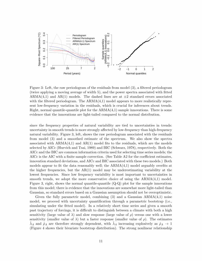
Figure 3: Left, the raw periodogram of the residuals from model (3), a filtered periodogram(twice applying a moving average of width 5), and the power spectra associated with fittedARMA(4,1) and AR(1) models. The dashed lines are at ±2 standard errors associatedwith the filtered periodogram. The ARMA(4,1) model appears to more realistically repre-sent low-frequency variation in the residuals, which is crucial for inferences about trends.Right, normal quantile-quantile plot for the ARMA(4,1) sample innovations. There is someevidence that the innovations are light-tailed compared to the normal distribution.
since the frequency properties of natural variability are tied to uncertainties in trends:uncertainty in smooth trends is more strongly affected by low-frequency than high-frequencynatural variability. Figure 3, left, shows the raw periodogram associated with the residualsfrom model (3) and a smoothed estimate of the spectrum. We also show the spectraassociated with ARMA(4,1) and AR(1) model fits to the residuals, which are the modelsselected by AICc (Hurvich and Tsai, 1989) and BIC (Schwarz, 1978), respectively. Both theAICc and the BIC are common information criteria used for selecting time series models; theAICc is the AIC with a finite sample correction. (See Table A2 for the coefficient estimates,innovation standard deviations, and AICc and BIC associated with these two models.) Bothmodels appear to fit the data reasonably well; the ARMA(4,1) model arguably overfits atthe higher frequencies, but the AR(1) model may be underestimating variability at thelowest frequencies. Since low frequency variability is most important to uncertainties insmooth trends, we adopt the more conservative choice of using the ARMA(4,1) model.Figure 3, right, shows the normal quantile-quantile (Q-Q) plot for the sample innovationsfrom this model; there is evidence that the innovations are somewhat more light-tailed thanGaussian, so standard errors based on a Gaussian assumption should not be overoptimistic.
Given the fully parametric model, combining (3) and a Gaussian ARMA(4,1) noisemodel, we proceed with uncertainty quantification through a parametric bootstrap (i.e.,simulating under the fitted model). In a relatively short time series and given a smoothpast trajectory of forcings, it is difficult to distinguish between a climate with both a highsensitivity (large value of λ) and slow response (large value of ρ) versus one with a lowersensitivity (smaller value of λ) but a faster response (smaller value of ρ). The estimatesλA and ρA are therefore strongly dependent, with λA increasing explosively as ρA → 1(Figure 4 shows their bivariate bootstrap distribution). The strong nonlinear relationship
11

●●
●
●
●
●●
●●●
●●
●
●
●●
●
●
●
●
●
●
●
●
●
● ●
●
●
●
●
●
●
● ●
●
●
●
●
●●●●●
●
●
●
●
●
●●
●
●
●
●
●
● ●
●
●
●
●
●
●
●
●
●
●●●
●
●
●●●●
●
●
●
●●
●
●
●
●
●
●
●
●
●●
●●
●● ●
●
●
●
●
●
●
●
●
●
●
●
●
●
●
●
●
●●
●●
●
●●
● ●
●●
●
●●
●
●
●
●● ●
●●
●
●
●●
●
●
●
●●
●
● ●
●
●
●
●
●●●
●
●
●
●
●
●
●
●
●
●
●
●
●
●●
●
●●
●
●
●
●
●● ●
●
●
●
●
●
●
●
●
●●
●●
●●
● ●
●● ●
●
●
●●●
●
●●
●
●
●●
●
●
●
●●
●
●
●
●
●
●● ●
●
●
●
●
●
●
●●
●
●
●
●●
●
●
●
●
●
●
●
● ●
●●
●
●
●
●
●
●
●●
●●
●
●
●●
●
●
●
●
●
●●●●●
● ●
●
●●●
●●
●
●
●
●
●
●
●
●
●
●
●
●
●
●
●
●
●
●●
●●
●
●
●
●
●●●
●
●
●
●
●
●
●
●
●
●
●●●
●
●●
●
●
●
●●
●●
●
●
●
●
●
●
●
●
●
●
●
●
●●
●
●
●
●●
●
●
●
●
●
●●
●
●
●
●
●
●
●
●
●
●
●●
●
●
●
●●
●●
●
●
●
●
●
●
●●
●
●●
● ●●
●
●
●●
●
●
●
●
●●
●
●●
●
●
●
●
●
●
●
●
●
●
●
●
●
●
●
●
●●
●
●
● ●
●
●
●
●
●
●●
●
●
●
●
●
●
●●
●●
●
●
●
●
●
● ●
●
●
●
●
●
●
●
●
●●
●●
●
●
●
●●
●
●●
●
● ●●
●
●
● ●
●
●
●
●
●
●●
●
●
●
●
●
●
●
●●
●
●
●●
●
●
●
●
●
●●
●●
●
●
●
●
●
●
●
●●
●
●
● ●●
●
●
●●
●
● ●
●●
●
●
●●●
●
●
●
●
●
●●
●
●●
●
●
●
●
●
●
●
●
●
●
●
●
●
●
●
●
●
●
●
●
●
●
●
●
●●
●
●
●●
●
●
●
●
●
●
●
●
●
●●
●
●
●
●●●
●
●
●
●●
●
●
●
●●
●
●
●
●●●
●
●
●●
●
●
●
●
●
●
●●
●
●
●●
●
●
●
●
●
●
●●
●
● ●
●
●
●●
●
●
●
●
●
●
●
●
●
●
●
●
●
●●
●
●
●
●●●
● ●
●●
●●
●●
●
●●
●
●
●
●
●●
●
●
●
●
●●
●
●
●
●
● ●
●●
●
● ●
●
●
●●
●
●
●
●
● ●
●●
●
●
●●
●
●
●
●
●
●●
●
●
●●
●
●
●●
●
●
●
●
●
●
●●
●
●●
●
●
●
●
●
● ●
●
●●
● ●
●
●●
●● ●
●
● ●●
●●
●
●●
●●
●
●●●●
●●
●
●
●
●
●
●
●
●
●
●
●
●
● ●
●●
●
●
●
●
●
●
●
●
●
●
● ●
●
●
●
●●
●
●
●●●
●
●
●
●●●●
●
●
● ●
● ●
●●
●
●
●
●
●
●
●
●
●
●
●
●
●
●
●
●
●
●
● ●
●
●●
●
●
●
●
●●●
●
●
●
●●●
●
●
●
●
●●
●
● ●
●
●
●
● ●
●
●
●
●
●
●
●
●
●
●
●●● ●
●
●
●
●
●
●●
●●
●
●●
●
●
●
●
●
●
●●●
●
●
●
●
●
●
●
●●
●
●
●
●●
●
●●
●●
●●
●
●
●●●
●●●
●●
●
●
●
●●
●
●
●●
●●
●
●●●
●
●
●
● ●
●
●
●
● ●●
●●●
●
●
●
●●
●
●
●
●
●
●●
●
●
●
●●
●
●●
●
●● ●
●
●●
●●
●
●● ●
λ A (
°C p
er d
oubl
ing)
ρA
1e−04 0.001 0.01 0.1 0.5 0.9 0.99 0.999 0.9999
1.25
2.5
510
100
1000
annual decadal centennial millenial
Figure 4: Distribution of the parametric bootstrap estimates of λA and ρA from model (3).It is difficult to distinguish between the rate of response and the sensitivity using onlyglobal mean temperatures from recent history.
between these two parameters, and the high degree of skewness in the marginal distributionof λA, are the reasons that we rely on bootstrapping for uncertainty quantification, as thetypical appeals to asymptotic normality are not viable in this setting.
In the following, we will represent uncertainties using the simple bootstrap percentilemethod. The percentile method is subject to criticism (e.g., Hall (1988)). We have found,however, that adjusting the percentile method using a nested bootstrap results in narrowerconfidence limits. For this reason, we believe that the raw percentile-based intervals maybe conservative in this setting, so we choose to report the apparently conservative intervals.Our point estimates are based on a two-step procedure wherein model (3) is estimated vialeast squares and the ARMA(4,1) model is estimated via maximum likelihood on the resid-uals. While this procedure may be somewhat suboptimal compared to jointly estimatingthe mean and covariance structure, the two-step procedure is substantially faster, which isimportant for carrying out the nested bootstrap.
4.1 Uncertainties in the sensitivity parameters
When using the full 1880-2015 global mean surface temperature record, the point estimatefor the sensitivity to anthropogenic forcing is λA = 1.8◦C per doubling, with ρA = 0.80(which implies mixing on decadal timescales). The estimated sensitivity to natural forcingis much smaller, λN = 0.21◦C per doubling with ρN = 0.58. In this section, we discussuncertainties in these estimates.
Using our statistical model, the historical data appear to provide a lower bound for λA(assuming for now that the forcings are known) but cannot rule out extremely large and
12

λA = 1.8 λN = 0.80Percentile interval Lower Upper Lower Upper
5-95 (90%) 1.5 3.0 -0.15 1.52.5-97.5 (95%) 1.5 690 -1.1 4.10.5-99.5 (99%) 1.4 790 -13 490
Table 1: Parametric bootstrap percentile intervals for the sensitivities in model (3), λA andλN , to anthropogenic and natural sources, respectively (in units ◦C per doubling). Thedata appear to provide a lower bound for λA, but cannot rule out even implausibly largevalues; the very large values are associated with slow responses (see Figure 4). The datacannot rule out λN = 0, likely because there are few prominent volcanic eruptions in thehistorical record analyzed and the response to volcanic aerosols may be small.
implausible values on the order of tens or hundreds of degrees per doubling (the 2.5-97.5thbootstrap percentile interval is 1.5 to 690◦C per doubling). These very large values are notsupported by evidence from the paleoclimate record (e.g., IPCC (2013) Chapter 5) and theapproximation of the linear forcing feedback model, on which (3) implicitly relies, breaksdown under high sensitivity (Bloch-Johnson et al., 2015). For the sensitivity to naturalforcings, the data cannot rule out λN = 0 (the 2.5-97th bootstrap percentile interval is-1.1 to 4.1◦C per doubling). Table 1 gives some intervals at different percentiles for theparameters λA and λN . (The parameters ρA and ρN are essentially unconstrained by thedata.)
The IPCC’s own 66% “likely” interval for equilibrium sensitivity is 1.5◦C to 4.5◦Cper doubling, which subjectively combines estimates from various sources using multiplelines of evidence including from ensembles of models with different physics, and accountsfor other sources of uncertainty that we have so far ignored, such as uncertainty in theforcings themselves (see IPCC (2013) 10.8.2 and Box 12.2). The bulk of the distributionof our estimate is somewhat narrower than the IPCC’s, likely because so far we have notaccounted for uncertainty in radiative forcings; however, the IPCC rules out the very largeand unphysical values in the right tail of our intervals. We here stress again that since weare estimating the centennial-scale response, the estimates of the sensitivity that we providewill tend to be lower than the equilibrium sensitivity estimated in the IPCC’s interval (seeAppendix A1). Individual estimates of the equilibrium climate sensitivity and associateduncertainty in the literature are discussed in IPCC (2013) Section 10.8.2 (see also againAppendix A1).
The main source of uncertainty in the upper bound for λA is due to uncertainty inthe “equilibration time” of the climate associated with smoothly increasing anthropogenicforcing, controlled by ρA. If we restrict ρA to, say, centennial scales or smaller, then theuncertainty is substantially decreased (see again Figure 4). While we may argue throughother lines of evidence and reasoning that extremely large values of ρA and λA are implausi-ble, the statistical model is being used to quantify the information content of the historicaltemperature record itself. This suggests that even our minimally informed model may beoverly empirical for some purposes. The inability of the data to rule out λN = 0 is, on theother hand, probably due to the fact that there are few prominent volcanic eruptions in thehistorical record analyzed and that the response to volcanic aerosols may be small for the
13

reasons discussed above.
4.2 Uncertainties in near- and long-term trends
The uncertainties in the sensitivity and rate of response parameters imply greater uncer-tainties in projected longer-term future trends in global mean temperature than in thehistorical and near-term projected trends. To illustrate this, we examine the implied fu-ture trends under the hypothetical (extended) RCP8.5 scenario, in which radiative forcingincreases and then stabilizes in the year 2150. We simulate new time series using our es-timates of model (3) and the ARMA(4,1) noise model, given radiative forcings from thisscenario. The projected trend and associated pointwise uncertainties are shown in Figure 5.
Projected mean temperatures, and especially their associated uncertainties, continue toincrease even after stabilization of forcing. This is a consequence of the joint uncertaintyin λA and ρA, and in particular of the inability to rule out implausible values of theseparameters. If the goal, then, is to provide a long-term projection of mean temperaturesgiven only the historical temperature record, these estimates will unsurprisingly be quiteuncertain (even assuming known past and future forcings).
On the other hand, trends in the historical and near-term response are much morecertain. The observations strongly suggest that mean temperatures increased in the 20thcentury: for example, the (2.5-97.5)-percentile interval for the mean response in the year2000 (expressed compared to the 1951-1980 average) is well above zero at (0.4,0.6)◦C. Thesekinds of distinctions between the uncertainty in the near- and longer-term mean responsesare not easily made using a time trend model.
4.3 Decreasing uncertainty in the sensitivity parameter as more data isobserved
We have shown that the short historical temperature record alone produces fairly uncertainestimates of the sensitivity parameter, λA in model (3) (Figure 4, Table 1), and thereforeof longer-term temperature trends (Figure 5). We now examine how these uncertaintiesdecrease as the temperature record increases (as in, e.g., Kelly and Kolstad (1999); Ringand Schlesinger (2012); Padilla et al. (2011); Urban et al. (2014); Myhre et al. (2015)and others). To do this, we artificially extend the temperature record by generating newsynthetic time series using the mean and noise models estimated from the historical data andforcings from the same RCP8.5 scenario described above. We then reestimate model (3) foreach synthetic series, using successively longer synthetic datasets. The results suggest thatthe data will not constrain the upper bound on the sensitivity parameter until another ∼50years, by which time (under our estimated model and the RCP8.5 scenario) temperatureswill have already risen by about 3◦C from the preindustrial climate. A summary of theevolution of uncertainties is given in Table 2.
These estimates could be more strongly constrained by using additional physical in-formation. As discussed previously, the very high sensitivity estimates in the bootstrapdistribution are cases where the estimated response time is unphysically long. Withoutexternal information about this timescale, however, long data records are required to ruleout the large values of ρA and λA that the model entertains.
14

Year
Tem
pera
ture
Ano
mal
y (°
C)
1900 2000 2100 2200 2300
05
1015
2025
30
Figure 5: Projected mean temperature anomalies, and their uncertainties, under theRCP8.5 scenario, based on estimates from model (3) and assuming ARMA(4,1) noise. Theblack curve shows the observed temperatures. Intervals are pointwise (2.5-97.5)-percentileintervals. Radiative forcing stabilizes in the year 2250, but mean temperatures and espe-cially their uncertainties continue to increase. While uncertainties in the long-term responseare quite large, due largely to the inability to rule out implausible values of λA, the historicaland near-term response is much more certain.
End year(2.5-97.5)th percentile Change in mean(◦C per doubling) from preindustrial (◦C)
2025 (1.5, 16) 1.32050 (1.6, 11) 2.22075 (1.6, 2.8) 3.12100 (1.7, 2.0) 3.9
Table 2: Evaluation of how uncertainty in the sensitivity parameter, λA, decreases asmore data is observed, from simulations under the RCP8.5 scenario of future radiativeforcing with an assumed value of λA = 1.8◦C per doubling. The middle column showsthe (2.5-97.5)th-percentile intervals for λA from simulations under the fitted model (3) andARMA(4,1) noise. The rightmost column shows the increase in mean temperatures fromthe preindustrial climate under the fitted model at the year in question. Uncertainties inthe upper bound of λA decrease relatively slowly as more data is observed.
15
4.4 Is there evidence of long memory natural variability in global meantemperatures?
One of the complicating factors in estimating trends in climate time series is the questionof whether global mean temperatures exhibit long memory. Long memory processes havepower spectra that behave like (2 sin(ω/2))−2d as the frequency ω → 0, with d > 0 (i.e.,infinite power at the frequency zero); when d < 1 the process has finite total variance,as would be expected for a variable like global mean temperature. For more details onlong memory processes, see Beran et al. (2013). By contrast, short-memory processes(like the ARMA(4,1) model we assume), have finite power at the origin. Many authorshave suggested that natural temperature variability is well-modeled by processes with longmemory but finite variance (e.g., Bloomfield (1992), Smith and Chen (1996), Gil-Alana(2005), Lennartz and Bunde (2009), Løvsletten and Rypdal (2016), and many others). Someauthors have made a stronger claim that global mean temperatures are well-modeled by arandom walk (e.g., Gordon (1991) and at least one standard time series textbook, Shumwayand Stoffer (2013)), which would imply that global mean temperatures do not have a finitevariance over time. In either case, if the Earth’s temperatures exhibited long memory,it would be more difficult to estimate trends than in the short memory case, since low-frequency variability can be difficult to distinguish from trends.
The evidence for long memory, however, strongly depends on the assumed trend model.Many of the aforementioned authors draw their conclusions by assuming a linear time trendmodel and applying that model to the temperature record on durations of decades to overa century. As discussed previously, a linear trend model applied to a time series with anonlinear trend will imply excessive low-frequency noise. Figure 6 shows the periodogramsof the residual global mean temperatures after removing either a linear time trend or a trendof the form of (3). While the high-frequency behavior of the residuals is not much affectedby the choice of trend model, the low-frequency behavior is very much affected. Apparentlow-frequency variability is made more severe by assuming that mean temperatures increaselinearly in time.
The question of long memory cannot be definitively settled using a dataset of only 136observations, and other analyses make use of longer climate model runs or the paleoclimaterecord (e.g., Mann (2011)). Nevertheless, it should be clear that the linear time trend modelis especially problematic for this purpose. In general, regression models in time, linear orotherwise, have a danger either of mistaking systematic trend for apparent low frequencyvariability (as just described), or of mistaking low-frequency variability for systematic trend(as would occur, for example, when using a nonparametric regression with too small of asmoothing bandwidth). Either can lead to misstated uncertainties, and therefore can beproblematic even if the claim is that the trend model is only being used to test for significantwarming and that the model is not believed to be true.
4.5 Implications of uncertain inputs: radiative forcing and temperatures
The analysis thus far has assumed that both radiative forcings and temperatures are knownexactly, but uncertainty in the sensitivity and in trends also propagates from uncertaintyin these quantities. We therefore discuss at least roughly the potential implications ofimperfect knowledge of these inputs.
Of the two factors, uncertainty in radiative forcings, particularly from aerosols, is more
16

Period (years)
Squ
are−
Roo
t Per
iogr
am (
°C)
100 25 7 20.
00.
20.
40.
60.
8
Linear trendModel (3)
Figure 6: Raw periodograms of residuals from models (2) (dashed) and (3) (solid) fit to thefull data record. There is substantially more low-frequency variability in the residuals fromthe linear trend model than in the residuals from model (3). Misspecified mean modelswill give a misleading impression of low-frequency variability, and therefore misleadinguncertainties associated with the mean trend.
consequential, especially for the inferred lower bound of the sensitivity parameter frommodel (3). The importance of radiative forcing uncertainty for uncertainties in climatesensitivity has been widely noted (e.g., Gregory and Forster (2008); Padilla et al. (2011);Otto et al. (2013); Masters (2014); Lewis and Curry (2015); Myhre et al. (2015)). Thetrajectory of net effective radiative forcing from anthropogenic sources is poorly known;the IPCC states that the difference in net effective radiative forcing from anthropogenicsources between the years 2011 and 1750 was about 2.29 W/m2 with a 95% confidenceinterval of 1.13 to 3.33 W/m2. We explore the implications of this uncertainty by simplyscaling the entire trajectory of net radiative forcings from 1750 to the present such thatthe uncertainty in 2011 is as stated. Adjusting aerosol forcings to the high or low ends,respectively, produces sensitivity estimates from (3) varying by over a factor of two, from1.2 to 3.7◦C per doubling (vs. the original estimate 1.8◦C). The aerosol uncertainty appearsimportant: the value 1.2◦C per doubling is lower than all of the bootstrap values of λAgenerated assuming known forcings (Figure 4 and Table 1).
Uncertainties in the global mean surface temperature record are comparatively lessimportant. To partially address this issue, we re-estimate model (3) using each of the100 ensemble members of the HadCRUT4 global mean temperature ensemble. The pointestimates of λA range from 1.5 to 2.1◦C per doubling, with estimates of ρA ranging from0.79 to 0.90. The point estimates of λN range from 0.71 to 20◦C degrees per doubling,with estimates of ρN ranging from 0.86 to 0.996. The additional uncertainty induced byobservational uncertainty in the temperature record is smaller than either the uncertaintyinduced by natural variation in the temperature record or the uncertainty in radiativeforcings.
17

5 Parametric vs. nonparametric uncertainty quantification
In Sections 3 and 4, we showed that characterizing the Earth’s systematic temperatureresponse is better informed by making physical assumptions than by an ostensibly moreempirical approach. In this section, we ask a similar question about characterizing naturalvariability, in settings similar to that discussed where data are temporally correlated andlimited in length. We used a Gaussian ARMA(4,1) noise model in Section 4: is it morerobust to assume a model for the noise, as we have done, or to adopt a nonparametricapproach? The answer to this question depends on the length of the data record and thenature of the natural variability.
For the purposes of this illustration, we will use not the actual temperature record butrather some simple synthetic examples. We consider several artificial, trendless time series(the true mean of the process is constant) with temporally correlated noise, and evaluatethe results of testing for a linear time trend (i.e., fitting model (2) and testing againstthe null hypothesis that β = 0) using different parametric (both correctly specified andnot) and nonparametric methods for estimating uncertainties. The ordinary least squaresstandard errors, which assume uncorrelated noise, tend to be anticonservative (too small)and time series methods are supposed to ameliorate this overconfidence, but may or maynot be successful in this regard depending on the context. The illustrations are simple butour conclusions should be relevant to actual data analysis and to more informed models.
We consider a few parametric approaches common in time series analysis. The typicalpractice is to assume that the noise follows a low order model, such as an ARMA model.Ideally, the noise model would be chosen in consultation with diagnostic plots and aninformation criterion like the AICc (as we do in Section 4). However, it is common practiceto automatically select a model either solely by minimizing the AICc or another criterion,or just to assume a simple time series model, often the AR(1) model. Uncertainty in thetrend parameter(s) can then be estimated in several ways. Usually, this is done assumingasymptotic normality for maximum likelihood estimators, and a test might be carried outusing a t-statistic. If asymptotic normality is not viable, as for model (3), an alternative isto resort to using a parametric bootstrap (again as we do in Section 4) and to perform thetest using bootstrap p-values.
We also evaluate the perhaps most typical nonparametric method for accounting for de-pendence in a time series, the block bootstrap (Kunsch, 1989). Here, residuals are resampledin blocks to generate bootstrap samples that retain much of the dependence structure in theoriginal data. A popular variant is the circular block bootstrap (Politis and Romano, 1992),in which blocks can be overlapping and blocks starting at the end of the time series wrapback to the beginning. The block bootstrap has been a common method in the climate andatmospheric sciences for at least two decades (Wilks, 1997) and has been applied previouslyto test for time trends (or changes thereof) in the global mean surface temperature record.For example, Rajaratnam et al. (2015) argue that the circular block bootstrap gives betteruncertainty estimates than does a parametric analysis in the setting of testing for a trendin a 16-year segment of the global mean temperature record.
While the block bootstrap works very well in some settings, the procedure is not free ofassumptions. Like other variants of the nonparametric bootstrap, its justification is basedon an asymptotic argument: for the block bootstrap to work well, the size of the block hasto be small compared to the overall length of the data but large compared to the scale ofthe temporal correlation in the data. When the overall data record is short and natural
18

variability is substantially positively correlated in time, as for the historical temperaturerecord, these dual goals may not both be achieved and we should not expect the blockbootstrap to perform well.
In the following, we compare five methods (four parametric and one nonparametric) forgenerating nominal p-values testing for a significant linear time trend in trendless syntheticdata: (a) a t-test assuming independent noise, (b) a t-test assuming Gaussian AR(1) noisewith the model estimated via maximum likelihood, (c) bootstrap p-values from a parametricbootstrap assuming Gaussian AR(1) noise, (d) a t-test assuming Gaussian ARMA(p,q) noisewith the order chosen by minimizing AICc, and (e) bootstrap p-values from a circular blockbootstrap. We generate synthetic data from three different time series models, but in cases(b) and (c), the assumed parametric model is always AR(1). (Table A3 summarizes themodels from which we simulate.) In cases (a), (b), and (d), the t-test degrees of freedomare approximated by n−2 minus the number of parameters in the noise model. In case (e),we estimate p-values using a few different block lengths and show the results most favorableto the block bootstrap.
After generating nominal p-values, we evaluate the performance of the different methods.Since the null hypothesis is true in this artificial setting (the synthetic series are trendless),a correct p-value would be uniformly distributed. Deviations from the uniform distributionwould then be a sign that the procedure generating the nominal p-value is uncalibrated. Wetherefore use Q-Q plots to compare the distribution of the simulated nominal p-values withthe theoretical uniform distribution. Uncertainties are underestimated when the nominalp-value quantiles are smaller than the theoretical quantiles (i.e., when the Q-Q plot is belowthe one-to-one line). In this situation, inferences are anticonservative and the tests usingthe selected method will have Type I error rates that are larger than the nominal rate.
5.1 Parametric vs. nonparametric methods under a correctly specifiednoise model
We first compare the performance of the five methods for generating nominal p-values in thesetting where the assumed AR(1) model is correctly specified (Figure 7). Unsurprisingly,pre-specified parametric time series methods give reasonably calibrated inferences whenthe parametric model is correctly specified (Figure 7, rows 2 and 3), although maximumlikelihood gives somewhat anticonservative estimates of uncertainty with small sample sizes.The anticonservative bias of the maximum likelihood estimator can be reduced by insteadusing restricted maximum likelihood (REML) (e.g., McGilchrist (1989)) (see Applendix A5),but we focus here on the performance of maximum likelihood because it is more usuallythe procedure employed. It is also unsurprising that p-values under assumed independenceare quite uncalibrated and anticonservative in this setting (Figure 7, top row), becausestandard errors are underestimated when positive temporal correlation is ignored.
It may, on the other hand, be surprising that automatically chosen parametric methodsand nonparametric methods (blind selection via AICc and the block bootstrap, Figure 7,rows 4 and 5) can perform even more poorly than assuming independence if the samplesize is very small. The AICc does improve on the AIC (not shown) by attempting toaccount for small sample biases, but still performs poorly in very small samples. The(nonparametric) block bootstrap is the worst-performing method at the smallest samplesizes while ostensibly based on the weakest assumptions. For either of these methods toperform comparably to the pre-specified parametric methods, sample sizes must be quite
19

n=15
p−
valu
e qu
antil
e
n=30 n=60
uniform quantile
n=120 n=240
OLS
t−
test
AR
(1)
t−te
stP
aram
etric
Boo
tstr
ap(A
R(1
) no
ise)
AR
MA
(p,q
)t−
test
Blo
ckB
oots
trap
Figure 7: Quantile-quantile plots comparing the distribution of nominal p-values to thetheoretical uniform distribution. Simulations are of mean zero, Gaussian AR(1) time seriesand p-values correspond to a two-sided test for a linear time trend. The length of thetime series is given above each column. In the first row, the p-values are from the OLSt-test assuming independent noise; the second row is the t-test assuming AR(1) noise andthe model fit via maximum likelihood; the third row uses a parametric bootstrap (againassuming AR(1) noise); the fourth row uses a t-test assuming ARMA(p,q) noise with theorder of the model selected by AICc; and the last row uses a circular block bootstrap withblock size chosen to be favorable to this method. The p-values calculated assuming thecorrect parametric model appear approximately correct for modest sample sizes and alwaysoutperform both blind selection by AICc and the block bootstrap. The latter two methodscan be worse than assuming independence when sample sizes are very small.
large, indeed in this illustration larger than the available global mean temperature record.This should serve as a warning against using these methods for time series of modest length.
In actual practice, it can be advantageous, as we already discussed, to choose a noisemodel not automatically but in consultation with diagnostics (such as by comparing the-oretical spectral densities with the empirical periodogram). In Section 4, we chose a noisemodel with consideration for the model’s representation of low-frequency variability. Inthat example, the chosen model did minimize the AICc, but gave more conservative in-ferences than the AR(1) model (which was chosen by BIC). The illustration above showsthat this behavior is not generically true and that for small sample sizes it is dangerous toblindly select models by minimizing an information criterion alone.
5.2 Parametric vs. nonparametric methods under a misspecified model
The comparisons in the previous section were too favorable to the pre-specified parametricmethods because the order of the specified noise model (an AR(1) model) was known to
20

ARMA(1,1)
Frequency
Squ
are−
Roo
t Spe
ctru
m0.0 0.1 0.2 0.3 0.4 0.5
0.0
1.0
2.0
3.0
Fractionally−differenced AR(1)
Frequency
0.0 0.1 0.2 0.3 0.4 0.5
01
23
45
67
True SpectrumBest AR(1) Approximation
Figure 8: The power spectra associated with the two models from which we generatesynthetic time series in Section 5.2, along with spectra of the best AR(1) approximations(in Kullback-Leibler divergence) to both models; see Table A3 for noise model parameters.The corresponding illustrations of the performance of the various time series methods areshown in Figures 9 and 10. The AR(1) model will tend to overestimate low-frequencyvariability in the first case and underestimate it in the second.
be correct. Now we compare these methods when the assumed noise model is misspecified.The performance of misspecified methods will depend in particular on how the misspeci-fied model represents low- versus high-frequency variations in the noise process. Modelsthat underestimate low-frequency variability will tend to be anticonservative for estimatinguncertainties in smooth trends, whereas those that over-estimate low-frequency variabilitywill tend to be conservative. We therefore repeat the illustrations in the previous sectiongenerating the synthetic time series from two different noise models (but still using thepre-specified AR(1) model to generate nominal p-values). The two models are chosen sothat their best AR(1) approximations either under- or over-represent low-frequency vari-ability. (Figure 8 shows the spectra corresponding to these two noise models and the bestAR(1) approximation to each. See the Appendix, Table A3, for the model parameters andSection A3 for a comparison under an additional misspelled model.) The Q-Q plots corre-sponding to how the various time series methods perform in these two settings are shownin Figures 9 and 10.
First, we consider an ARMA(1,1) process whose best AR(1) approximation over-representslow-frequency variability (Figure 9). The results are similar to those when the model wascorrectly specified, except that at the largest sample sizes the pre-specified parametricmethods slightly overestimate uncertainties, for the reasons discussed above. As before,both blind selection via AICc and the block bootstrap perform well for large sample sizesbut very poorly for the smallest sample sizes.
Second, we consider a fractionally integrated AR(1) process; because this is a long-memory process, the best AR(1) approximation (and indeed any ARMA model) will severelyunder-represent low-frequency variability (Figure 10). All of the methods struggle in thissetting and produce anticonservative estimates, but the pre-specified parametric methodsstill typically perform better than the ostensibly more flexible methods.
These results confirm that approaches to representing noise that appear to weakenassumptions are not guaranteed to outperform even misspecified parametric models. Mis-
21

n=15
p−
valu
e qu
antil
e
n=30 n=60
uniform quantile
n=120 n=240
OLS
t−
test
AR
(1)
t−te
stP
aram
etric
Boo
tstr
ap(A
R(1
) no
ise)
AR
MA
(p,q
)t−
test
Blo
ckB
oots
trap
Figure 9: Same as Figure 7 but with simulations from an ARMA(1,1) model. The p-valuescalculated by incorrectly assuming an AR(1) model are increasingly conservative in largersample sizes in this setting. Both blind selection via AICc and the block bootstrap areanticonservative for small sample sizes but improve as the sample size increases.
n=15
p−
valu
e qu
antil
e
n=30 n=60
uniform quantile
n=120 n=240O
LS t
−te
stA
R(1
) t−
test
Par
amet
ricB
oots
trap
(AR
(1)
nois
e)
AR
MA
(p,q
)t−
test
Blo
ckB
oots
trap
Figure 10: Same as Figure 7 but with simulations from a fractional AR(1) model. Whilenone of the methods perform very well here, the incorrectly specified parametric methodsare better, especially in smaller samples.
22
specified parametric models are most dangerous when low-frequency variability is under-represented, but methods like the block bootstrap will also have the most trouble whenlow-frequency variability is strong because very long blocks will be required to adequatelycapture the scale of dependence in the data. While it is crucial for the data analyst toscrutinize any assumed parametric model, we believe that in many settings when the timeseries is not very long, one will be better served by carefully choosing a low-order parametricmodel rather than resorting to nonparametric methods.
6 Discussion
We have shown that more targeted parametric modeling of trends and natural variabilitycan provide for more informative and reliable analyses of the global mean temperaturerecord than can more empirical methods. More empirical methods can fail to distinguishbetween systematic trends and natural variability, and can give seriously uncalibrated es-timates of uncertainty; this is particularly the case in the setting of analyzing historicaltemperatures, where the data record is relatively short and temporal correlation is rela-tively strong.
The model we use in our analysis provides insights about the information contained inthe historical temperature record relevant to both shorter-term and longer-term trend pro-jections. The limited historical temperature record can provide information about shorter-term trends but unsurprisingly cannot constrain long-term projections very well; the past136 years of temperatures simply do not alone contain the relevant information about equili-bration timescales that would be required to constrain long-term projections. (Our analysisconsiders globally averaged temperatures; use of spatially disaggregated data may providesome additional information.) The distinction between uncertainties in shorter-term andlonger-term projections, itself not easily made using a time trend model, serves to furtherillustrate that while the historical data record is an important source of information, italone cannot be expected to answer the most important questions about climate changewithout bringing more scientific information to bear on the problem.
The purpose of this paper has been to illustrate these ideas in a particular, importantscientific application. We believe that our discussion is illustrative of broader issues thatarise in applied statistical practice, and will have particular relevance to problems involvingtrend estimation in the presence of temporally correlated data and in relatively data-limitedsettings. We suspect that many readers having engaged in the practice of applied statisticshave felt personally the tension between targeted statistical modeling on the one handand more empirical analyses on the other. One lucid discussion of the broader issuessurrounding this tension can be found in the discussion of model formulation in Cox andDonnelly (2011). Empirical approaches have very successfully generated new insights andpredictions in important areas, but there is a wide range of scientific problems where theseapproaches do not perform well and where targeted, domain-specific modeling is required.Statisticians can provide important insights into scientific problems; a crucial role for thestatistician is to consider the modeling choices that will be both the most illuminating andthe most reliable given the scientific questions and data at hand.
23

References
Aldrin, M., M. Holden, P. Guttorp, R. B. Skeie, G. Myhre, and T. K. Berntsen (2012).Bayesian estimation of climate sensitivity based on a simple climate model fitted toobservations of hemispheric temperatures and global ocean heat content. Environ-metrics 23 (3), 253–271.
Armour, K. C., C. M. Bitz, and G. H. Roe (2013). Time-varying climate sensitivity fromregional feedbacks. Journal of Climate 26 (13), 4518–4534.
Arrhenius, S. (1896). On the influence of carbonic acid in the air upon the temperature ofthe ground. Philosophical Magazine Series 5 41 (251), 237–276.
Beran, J., Y. Feng, S. Ghosh, and R. Kulik (2013). Long-memory processes. New York:Springer.
Bloch-Johnson, J., R. T. Pierrehumbert, and D. S. Abbot (2015). Feedback temperaturedependence determines the risk of high warming. Geophysical Research Letters 42 (12),4973–4980.
Bloomfield, P. (1992). Trends in global temperature. Climatic change 21 (1), 1–16.
Cahill, N., S. Rahmstorf, and A. C. Parnell (2015). Change points of global temperature.Environmental Research Letters 10 (8), 084002.
Caldeira, K. and N. P. Myhrvold (2013). Projections of the pace of warming following anabrupt increase in atmospheric carbon dioxide concentration. Environmental ResearchLetters 8 (3), 034039.
Castruccio, S., D. J. McInerney, M. L. Stein, F. Liu Crouch, R. L. Jacob, and E. J. Moyer(2014). Statistical emulation of climate model projections based on precomputed gcmruns. Journal of Climate 27 (5), 1829–1844.
Cox, D. R. and C. A. Donnelly (2011). Principles of applied statistics. New York: CambridgeUniversity Press.
Easterling, D. R. and M. F. Wehner (2009). Is the climate warming or cooling? GeophysicalResearch Letters 36 (8), L08706.
Forest, C. E., P. H. Stone, and A. P. Sokolov (2006). Estimated pdfs of climate system prop-erties including natural and anthropogenic forcings. Geophysical Research Letters 33 (1),L01705.
Foster, G. and S. Rahmstorf (2011). Global temperature evolution 1979-2010. Environ-mental Research Letters 6 (4), 044022.
Geoffroy, O., D. Saint-Martin, D. J. L. Olivie, A. Voldoire, G. Bellon, and S. Tyteca(2013). Transient climate response in a two-layer energy-balance model. part i: Ana-lytical solution and parameter calibration using cmip5 aogcm experiments. Journal ofClimate 26 (6), 1841–1857.
24

Gil-Alana, L. A. (2005). Statistical modeling of the temperatures in the northern hemisphereusing fractional integration techniques. Journal of Climate 18 (24), 5357–5369.
Gluhovsky, A. (2011). Statistical inference from atmospheric time series: detecting trendsand coherent structures. Nonlinear Processes in Geophysics 18 (4), 537–544.
Gordon, A. H. (1991). Global warming as a manifestation of a random walk. Journal ofClimate 4 (6), 589–597.
Gregory, J. M. and P. M. Forster (2008). Transient climate response estimated from radia-tive forcing and observed temperature change. Journal of Geophysical Research: Atmo-spheres 113, D23105.
Gregory, J. M., R. J. Stouffer, S. C. B. Raper, P. A. Stott, and N. A. Rayner (2002).An observationally based estimate of the climate sensitivity. Journal of Climate 15 (22),3117–3121.
Hall, P. (1988). Theoretical comparison of bootstrap confidence intervals. The Annals ofStatistics 16 (3), 927–953.
Hansen, J., R. Ruedy, M. Sato, and K. Lo (2010). Global surface temperature change.Reviews of Geophysics 48 (4), RG4004.
Hansen, J., M. Sato, R. Ruedy, L. Nazarenko, A. Lacis, G. Schmidt, G. Russell, I. Aleinov,M. Bauer, S. Bauer, et al. (2005). Efficacy of climate forcings. Journal of GeophysicalResearch: Atmospheres 110 (D18).
Held, I. M., M. Winton, K. Takahashi, T. Delworth, F. Zeng, and G. K. Vallis (2010).Probing the fast and slow components of global warming by returning abruptly to prein-dustrial forcing. Journal of Climate 23 (9), 2418–2427.
Hurvich, C. M. and C.-L. Tsai (1989). Regression and time series model selection in smallsamples. Biometrika 76 (2), 297–307.
Huybers, P. (2010). Compensation between model feedbacks and curtailment of climatesensitivity. Journal of Climate 23 (11), 3009–3018.
IPCC (2013). Climate Change 2013: The Physical Science Basis. Contribution of Work-ing Group I to the Fifth Assessment Report of the Intergovernmental Panel on ClimateChange. New York, NY: Cambridge University Press. Stocker, Thomas and Qin, Daheand Plattner, Gian-Kasper and Tignor, M and Allen, Simon K and Boschung, Judithand Nauels, Alexander and Xia, Yu and Bex, Vincent and Midgley, Pauline M (eds.).
Kelly, D. L. and C. D. Kolstad (1999). Bayesian learning, growth, and pollution. Journalof economic dynamics and control 23 (4), 491–518.
Knutti, R. (2008). Why are climate models reproducing the observed global surface warmingso well? Geophysical Research Letters 35 (18), L18704.
Kunsch, H. R. (1989). The jackknife and the bootstrap for general stationary observations.The Annals of Statistics 17 (3), 1217–1241.
25

Lennartz, S. and A. Bunde (2009). Trend evaluation in records with long-term memory:Application to global warming. Geophysical Research Letters 36 (16), L16706.
Lewis, N. and J. A. Curry (2015). The implications for climate sensitivity of ar5 forcingand heat uptake estimates. Climate Dynamics 45 (3), 1009–1023.
Liebmann, B., R. M. Dole, C. Jones, I. Blade, and D. Allured (2010). Influence of choiceof time period on global surface temperature trend estimates. Bulletin of the AmericanMeteorological Society 91 (11), 1485–1491.
Løvsletten, O. and M. Rypdal (2016). Statistics of regional surface temperatures postyear 1900. long-range versus short-range dependence, and significance of warming trends.Journal of Climate 29 (11), 4057–4068. in press.
Mann, M. E. (2011). On long range dependence in global surface temperature series.Climatic Change 107 (3), 267–276.
Marvel, K., G. A. Schmidt, R. L. Miller, and L. S. Nazarenko (2015). Implications forclimate sensitivity from the response to individual forcings. Nature Climate Change 6 (4),386–389.
Masters, T. (2014). Observational estimate of climate sensitivity from changes in the rate ofocean heat uptake and comparison to cmip5 models. Climate dynamics 42 (7), 2173–2181.
Mauritsen, T., B. Stevens, E. Roeckner, T. Crueger, M. Esch, M. Giorgetta, H. Haak,J. Jungclaus, D. Klocke, D. Matei, et al. (2012). Tuning the climate of a global model.Journal of Advances in Modeling Earth Systems 4 (3).
McGilchrist, C. (1989). Bias of ml and reml estimators in regression models with armaerrors. Journal of Statistical Computation and Simulation 32 (3), 127–136.
Meinshausen, M., S. J. Smith, K. Calvin, J. S. Daniel, M. Kainuma, J. Lamarque, K. Mat-sumoto, S. A. Montzka, S. C. B. Raper, K. Riahi, A. Thomson, G. J. M. Velders, andD. P. van Vuuren (2011). The rcp greenhouse gas concentrations and their extensionsfrom 1765 to 2300. Climatic Change 109 (1), 213–241.
Morice, C. P., J. J. Kennedy, N. A. Rayner, and P. D. Jones (2012). Quantifying uncer-tainties in global and regional temperature change using an ensemble of observationalestimates: The hadcrut4 data set. Journal of Geophysical Research: Atmospheres 117,D08101.
Myhre, G., O. Boucher, F.-M. Breon, P. Forster, and D. Shindell (2015). Declining un-certainty in transient climate response as co2 forcing dominates future climate change.Nature Geoscience 8 (3), 181–185.
Olivie, D. J. L., G. P. Peters, and D. Saint-Martin (2012). Atmosphere response time scalesestimated from aogcm experiments. Journal of Climate 25 (22), 7956–7972.
Otto, A., F. E. L. Otto, O. Boucher, J. Church, G. Hegerl, P. M. Forster, N. P. Gillett,J. Gregory, G. C. Johnson, R. Knutti, et al. (2013). Energy budget constraints on climateresponse. Nature Geoscience 6 (6), 415–416.
26

Padilla, L. E., G. K. Vallis, and C. W. Rowley (2011). Probabilistic estimates of transientclimate sensitivity subject to uncertainty in forcing and natural variability. Journal ofClimate 24 (21), 5521–5537.
Politis, D. N. and J. P. Romano (1992). A circular block-resampling procedure for stationarydata. In R. LePage and L. Billard (Eds.), Exploring the limits of bootstrap, pp. 263–270.New York: Wiley.
Rajaratnam, B., J. Romano, M. Tsiang, and N. S. Diffenbaugh (2015). Debunking theclimate hiatus. Climatic Change 133, 129–140.
Riahi, K., S. Rao, V. Krey, C. Cho, V. Chirkov, G. Fischer, G. Kindermann, N. Nakicenovic,and P. Rafaj (2011). Rcp 8.5–a scenario of comparatively high greenhouse gas emissions.Climatic Change 109 (1), 33–57.
Ring, M. J. and M. E. Schlesinger (2012). Bayesian learning of climate sensitivity i: Syn-thetic observations. Atmospheric and Climate Sciences 2 (4), 464–473.
Rose, B. E. J., K. C. Armour, D. S. Battisti, N. Feldl, and D. D. B. Koll (2014). Thedependence of transient climate sensitivity and radiative feedbacks on the spatial patternof ocean heat uptake. Geophysical Research Letters 41 (3), 1071–1078.
Santer, B. D., C. Mears, C. Doutriaux, P. Caldwell, P. J. Gleckler, T. M. L. Wigley,S. Solomon, N. P. Gillett, D. Ivanova, T. R. Karl, et al. (2011). Separating signal andnoise in atmospheric temperature changes: The importance of timescale. Journal ofGeophysical Research: Atmospheres 116, D22105.
Schwarz, G. (1978). Estimating the dimension of a model. The Annals of Statistics 6 (2),461–464.
Shumway, R. H. and D. S. Stoffer (2013). Time series analysis and its applications. NewYork: Springer.
Smith, R. L. and F.-L. Chen (1996). Regression in long-memory time series. In AthensConference on Applied Probability and Time Series Analysis, pp. 378–391. New York:Springer.
Sokolov, A. P. (2006). Does model sensitivity to changes in co2 provide a measure ofsensitivity to other forcings? Journal of climate 19 (13), 3294–3306.
Urban, N. M., P. B. Holden, N. R. Edwards, R. L. Sriver, and K. Keller (2014). Historicaland future learning about climate sensitivity. Geophysical Research Letters 41 (7), 2543–2552.
Wilks, D. S. (1997). Resampling hypothesis tests for autocorrelated fields. Journal ofClimate 10 (1), 65–82.
Winton, M., K. Takahashi, and I. M. Held (2010). Importance of ocean heat uptake efficacyto transient climate change. Journal of Climate 23 (9), 2333–2344.
27

A1 Implications for the transient climate response and equi-librium sensitivity
In this paper, we use the historical temperature record to estimate the trend model (3)that treats both the sensitivity parameter, λA, and the timescale of response parameter,ρA, as unknown. In this section, we compare our results to those from more commonlyused methods of inferring the climate response from projections in climate models and ofusing the historical temperature record to estimate a climate sensitivity parameter.
Model (3) is justifiable over the relatively short (centennial) timescales over which theso-called linear forcing-feedback model is applicable. The linear forcing-feedback model saysthat the mean temperature response to an instantaneous forcing F behaves like L∆T (t) ≈F − Q(t), where ∆T (t) is the change in mean temperature at time t from the baselinestate, Q(t) is the heat uptake (in W/m2) at time t, and L is a climate response parameter(with units W/m2/K). (In the context of this model, our sensitivity parameter is thenλA = F2×/L.) Our method essentially infers Q(t) by assuming that it decays exponentiallyuntil reaching zero again at equilibrium. The linear forcing-feedback model does not holdfor all time, however, in part because both feedbacks and rates of warming vary spatially. Inmodels, this typically results in additional warming over the millennial timescales on whichthe deep ocean mixes (e.g., Winton et al. (2010); Armour et al. (2013); Rose et al. (2014)and others). Additionally, climate feedbacks – and therefore climate sensitivity – may bestate-dependent; this effect also typically amplifies global mean temperature rise (Bloch-Johnson et al., 2015). Collectively, this suggests that our sensitivity parameter λA willbe smaller than the equilibrium climate sensitivity that measures the final, equilibriumtemperature response.
We can compare the results of our model to reported results from GCMs by estimatingthe transient climate response (TCR), a popular metric of the short-term temperature re-sponse to forcing in climate models. The TCR is defined as the change in mean temperatureafter 70 years of a CO2 concentration scenario that increases by 1% per year (so doublesafter 70 years). In a multi-model comparison of these centennial-scale projections, IPCC(2013) reports a 66% “likely” interval for the TCR of 1.0 to 2.5◦C. Our results from fittingmodel (3) to the historical data are fairly consistent with this: our estimate of the TCRis 1.7◦C, with the 2.5-97.5th bootstrap percentile interval of 1.2 to 1.9◦C. These intervalsare not strictly comparable because the IPCC’s subjectively combines information frommultiple lines of evidence. That said, our interval is shorter in part because it does notaccount for uncertainties in historical radiative forcings from anthropogenic aerosols. If werepeat the exercise of Section 4.5 (scaling the past radiative forcing trajectory), our centralestimate of the TCR would be about 1.2◦C if anthropogenic aerosols were on the high endand about 3.4◦C if on the low end.
We can also compare our estimate of λA to prior estimates of a sensitivity param-eter that also use the historical temperature record. The most typical approach in theliterature shares some commonalities with our method, beginning with the same linearforcing-feedback model that implicitly underlies our analysis, but estimating a sensitivityparameter by using an additional observational estimate of global heat uptake. That is,studies use estimates of changes in forcing, F ′, heat uptake Q′, and historical temperaturechange, ∆T ′, between a base a final period to compute L = (F ′ − Q′)/∆T ′ and thereforeλ = F2×∆T ′/(F ′−Q′). Studies using this method include Gregory et al. (2002), Otto et al.
28

StudyBest estimate 90% Interval
(◦C per doubling) (◦C per doubling)Energy balance
Gregory et al. (2002) 6.1 >1.6
model using Otto et al. (2013) 2.0 1.2-3.9temperatures, forcing Masters (2014) 2.0 1.2-5.2
and heat uptake Lewis and Curry (2015) 1.6 1.1-4.1
Trend model (3) this work 1.8 1.5-3.0
Table A1: Comparison of estimates of a sensitivity parameter from studies that use ob-servational data and a simple energy balance approach. The large best (median) estimatefrom Gregory et al. (2002) is due to a very fat right tail in their analysis; the mode of theirdistribution is 2.1◦C per doubling. The estimates given in these studies are similar to ourestimates of λA (which should be smaller than the equilibrium sensitivity).
(2013), Masters (2014), and Lewis and Curry (2015). The resulting sensitivity parameterestimate should be similar to our λA. Table A1 shows the results from these analyses.The uncertainty ranges given in these studies also tend to be slightly larger than the inter-vals we give for λA, again because these authors attempt to account for radiative forcinguncertainty in their analysis.
One advantage of this other, common approach is that it includes data about histori-cal heat uptake, which is an additional, albeit uncertain, source of information that mayimprove estimates. However, since these methods do not involve an explicit trend modeland require averaging the inputs over decadal or longer timespans, they cannot use thehistorical temperature record to estimate natural temperature variability. Most studiestherefore estimate natural variability using climate model output, but climate models donot perfectly realistically represent even global annual mean temperature variability.
By contrast, an advantage of our approach is that it allows one to use the historicaldata to understand natural variability. Additionally, our approach allows one to answerquestions about both historical trends and longer-term projections in the framework ofone statistical model, whereas the approaches discussed above do not allow one to infertrends from increasing-in-time forcing scenarios. A disadvantage of our approach is that,as discussed above, we rely on the historical global mean temperature record to estimatethe “equilibration” timescales (ρA and ρN ), but the data contain little information aboutthese quantities.
Regardless of the different advantages and disadvantages just discussed, both approachesto using the historical temperature record give similar results concerning the sensitivityparameter, and uncertainties in this parameter remain high. This demonstrates the limita-tions of the information content of the historical global mean temperature record alone forestimating longer-term projections of mean temperature changes. (As noted in Section 6,spatially disaggregated data may contain more information.)
A2 Coefficient estimates for noise model
Table A2 gives information about the ARMA(4,1) and AR(1) models fit to the residualsof model (3) used in Section 4. The ARMA(4,1) model give more conservative inferences
29

ModelAutoregressive Moving average Innovation
parameters parameter standardφ1 φ2 φ3 φ4 θ1 deviation (◦C) AICc BIC
ARMA(4,1)-0.29 0.36 0.05 0.24 0.80 0.09 -258 -242(0.19) (0.12) (0.09) (0.09) (0.19)
AR(1)0.52 – – – – 0.09 -257 -252
(0.07)
Table A2: Coefficient estimates (with standard errors in parentheses), innovation standarddeviations, and AICc and BIC associated with ARMA(4,1) and AR(1) fits to the resid-uals from model (3). These two models minimize AICc and BIC, respectively. We usethe ARMA(4,1) model because this model appears to better represent the low-frequencyvariation in the residuals (see Figure 3), which is crucial for inferences about trends.
Frequency
Squ
are−
Roo
t Spe
ctru
m
0.0 0.1 0.2 0.3 0.4 0.5
0.0
0.5
1.0
1.5
2.0
True AR(2) SpectrumBest AR(1) Approximation
Figure A1: The power spectra associated with the AR(2) model from which we generatesynthetic time series, along with spectrum of the best AR(1) approximation to each model(in Kullback-Leibler divergence); see Table A3 for noise model parameters.
about the systematic trend, and is the model we adopt in Section 4 (see Figure 3).
A3 Performance of misspecified methods under AR(2) sim-ulations
In Section 5.2, we compared the five methods for generating nominal p-values in two settingswhere the pre-specified AR(1) model was incorrect, where the AR(1) model either over- orunder-represented low-frequency variability. Here we present a third comparison, where thetrue noise model is an AR(2) model under which the AR(1) approximation over-representsvariability at the lowest frequencies but under-represents variability at intermediate frequen-cies (Figure A1 shows the true spectrum and the best AR(1) approximation and Table A3,last row, gives the model parameters).
In this setting, all methods perform better than in the setting of Figure 9, but the relative
30

n=15
p−
valu
e qu
antil
e
n=30 n=60
uniform quantile
n=120 n=240
OLS
t−
test
AR
(1)
t−te
stP
aram
etric
Boo
tstr
ap(A
R(1
) no
ise)
AR
MA
(p,q
)t−
test
Blo
ckB
oots
trap
Figure A2: Same as Figure 7 but with simulations from an AR(2) model. The relativeresults are similar to the setting of Figure 9 but all methods perform better here.
performance of the different methods is largely the same as there, except that selection byAICc now performs even more poorly than the block bootstrap at the smallest sample sizes(Figure A2). This behavior again serves to emphasize that when making inferences aboutsmooth trends, it is most crucial to represent low-frequency variability well.
A4 Model coefficients for simulations in Sections 5 and A3
In Sections 5 and A3, we generate synthetic, mean zero time series with different correlationstructures. The models that we simulate from are summarized in Table A3. The generalform for an autoregressive fractionally integrated moving average model (ARFIMA) of order(p, d, q) (of which all the simulated models are special cases) is(
1−p∑
k=1
φkBk
)(1−B)dYt = (1 +
q∑k=1
θkBk)ε(t),
where Yt is the time series at time t, the φ’s are the AR parameters, the θ’s are theMA parameters, d is the (fractional) differencing parameter, B is the backshift operator(i.e., BkYt = Yt−k), and ε(t) are uncorrelated innovations with constant variance. (Theconvention is that the acronym is shortened to account for parameters that are set to zero,so for example an ARFIMA(1,0,0) model is called an AR(1) model.)
31

Figure NameAR MA Differencing
parameter(s) parameter parameter7 AR(1) 0.5 0 09 ARMA(1,1) 0.5 0.25 010 fractional AR(1) 0.5 0 0.25A2 AR(2) (0.5,-0.25) 0 0
Table A3: Parameters in models from which we simulate in Sections 5 and A3.
n=15p
−va
lue
quan
tile
n=30 n=60
uniform quantile
n=120 n=240
AR
(1)
t−te
stM
LA
R(1
) t−
test
RE
ML
Figure A3: Comparison of maximum likelihood and REML in the same context as Figure 7.The first row is the same as the second row of Figure 7. In the second row here, theestimation is instead done using REML. The REML standard errors give better calibratedinferences in small sample sizes.
A5 Performance of maximum likelihood vs. REML
In Section 5, parametric inference was done using maximum likelihood estimators. Asshown there, the MLE for covariance parameters can give anticonservative estimates ofstandard errors for trend parameters in small sample sizes. This problem can be substan-tially ameliorated using restricted maximum likelihood (REML) instead. Figure A3 repeatsthe tests in Section 5.1 (where both the true and assumed models are AR(1)) and comparesthe performance of maximum likelihood and REML. For larger sample sizes, the two proce-dures are comparable, but in small sample sizes REML is much better calibrated (althoughstill slightly anticonservative in the smallest sample sizes).
32