estimation and elimination of power system harmonics...
TRANSCRIPT

Estimation and Elimination of Power System
Harmonics and Implementation of Kalman
Filter Algorithm
Anshuman Pradhan
711EE2067
Department of Electrical Engineering,
National Institute of Technology Rourkela

2 | P a g e
Estimation and Elimination of Power System
Harmonics and Implementation of Kalman
Filter Algorithm
Thesis submitted in partial fulfillment
of the requirements of the degree of
Dual Degree
In
Electrical Engineering
(Specialization: Power Electronics and Drives)
By Anshuman Pradhan
Roll No:711EE2067
Under the Guidance of Prof. Pravat Kumar Ray and Prof. Bidyadhar Subudhi
Department of Electrical Engineering,
National Institute of Technology Rourkela
3 | P a g e
Dept. of Electrical Engineering
National Institute of Technology, Rourkela.
Certificate
This is to certify that the thesis entitled, “Estimation and Elimination of
power system harmonics and implementation of Kalman Filter
Algorithm” submitted by Anshuman Pradhan in partial fulfillment of the
requirements for the award of dual degree (B. Tech and M. Tech degree)
at National Institute of Technology, Rourkela is an authentic work
carried out by him under my supervision and guidance. To the best of
my knowledge, the matter embodied in this Project review report has not
been submitted to any other university or institute for the award of any
Degree or Diploma.
Bidyadhar Subudhi Pravat kumar Ray
Dept. of Electrical Engg Dept. of Electrical Engg
National Institute of Technology National Institute of Technology
PLACE: Rourkela
DATE:

4 | P a g e
Declaration of Originality
I, Anshuman Pradhan, Roll Number 711EE2067 hereby declare that this dissertation
“Estimation and Elimination of power system harmonics and implementation of Kalman
Filter Algorithm” presents my original work carried out as a graduate student of NIT Rourkela
and, to the best of my knowledge, contains no material previously published or written by
another person, nor any material presented by me for the award of any degree or diploma of NIT
Rourkela or any other institution. Any contribution made to this research by others, with whom I
have worked at NIT Rourkela or elsewhere, is explicitly acknowledged in the dissertation.
Works of other authors cited in this dissertation have been duly acknowledged under the sections
“Reference”. I have also submitted my original research records to the scrutiny committee for
evaluation of my dissertation.
I am completely aware that in the case of any non-compliance detected in future, the
Senate of NIT Rourkela may withdraw the degree awarded to me on the basis of the present
dissertation.
Place: Rourkela Date:
Anshuman Pradhan Dept. of Electrical Engineering
National Institute of Technology, Rourkela

5 | P a g e
Acknowledgement
I would like to express my deepest gratitude to my project guide Prof. Bidyadhar Subudhi and
Prof. Pravat kumar Ray whose encouragement, guidance and support over the span of this work
enabled me to shape this project. His unending vitality and energy in examination had propelled
others, including me. Subsequently, the research work got to be smooth and remunerating for
me.
Besides, I would like to thank Prof. A.K. Panda, In-Charge of Power Electronics and Drives,
National Institute of Technology, Rourkela for his instrumental advice and for providing me with
an environment to complete my project successfully.
I am also deeply indebted to Prof.J.K. Satapathy, Head of the Department and all faculty
members of ElectricalaEngineering Department, National Institute of Technology, Rourkela, for
their contribution to my studies and research work. They have been incredible sources of
motivation to me, and I express my gratitude toward them.
To conclude, I take this opportunity to extend my deep appreciation to family and friends, for all
that they meant to me during the vital times of the conclusion of my project.
Place: Rourkela Date:
Anshuman Pradhan Dept. of Electrical Engineering
National Institute of Technology, Rourkela

6 | P a g e
Table of Contents
Certificate ............................................................................................................................................... 3
Declaration of Originality ......................................................................................................................... 4
Acknowledgement................................................................................................................................... 5
Table of Contents .................................................................................................................................... 6
LIST OF FIGURES ...................................................................................................................................... 8
ABSTRACT ............................................................................................................................................... 9
CHAPTER 1 ............................................................................................................................................ 10
INTRODUCTION ..................................................................................................................................... 10
1.1 Overview................................................................................................................................ 10
1.2 Motivation for Project Work ........................................................................................................ 11
1.2 Objectives of Project Work ..................................................................................................... 12
CHAPTER 2 ............................................................................................................................................ 13
INTRODUCTION TO HARMONICS AND SCHEMES TO REDUCE HARMONICS ........................................... 13
2.1 Power system frequency estimation: ........................................................................................... 13
2.2 Introduction: ................................................................................................................................ 13
2.3 Waveform distortion:................................................................................................................... 15
2.4 Creation and effects of harmonics: .............................................................................................. 16
2.4.1 Creation ................................................................................................................................ 16
2.4.2 Effects: .................................................................................................................................. 16
2.5 Methods of elimination of harmonics: ......................................................................................... 17
2.5.1 Harmonic Filters: ................................................................................................................... 19
2.6 Estimation of harmonics: ............................................................................................................. 20
CHAPTER-3 ............................................................................................................................................ 21
LITERATURE REVIEW.............................................................................................................................. 21
3.1 KALMAN FILTER ........................................................................................................................... 21
3.2 Kalman-Filtering Algorithm .......................................................................................................... 21
3.3 Shunt Active Power Filter ............................................................................................................. 23
3.4 Instantaneous Real and Reactive Power Theory (p-q method) ...................................................... 24
3.4.1 P-Q method Mathematical modelling .................................................................................... 25
3.5 Synchronous Reference Frame theory (d-q method) .................................................................... 26

7 | P a g e
3.5.1 D-Q method Mathematical modelling ................................................................................... 27
3.6 Hysteresis Current Controller ....................................................................................................... 28
CHAPTER-4 ............................................................................................................................................ 29
MATLAB/SIMULINK MODELLING AND RESULTS ..................................................................................... 30
4.1 Simulink modelawith Shunt Active PoweraFilter andaNon- linear burden .................................... 30
4.2 Simulink modelaof Shunt Active PoweraFilter witha‘p-q’ method ................................................ 31
4.3 Simulink model of Shunt Active Power Filter with ‘d-q’ method ................................................... 31
4.4 Design Parameters for MATLAB Simulation .................................................................................. 32
4.5 Simulink Results ........................................................................................................................... 32
4.5.1 Simulink Result with P-Q control strategy .............................................................................. 33
4.5.2 Simulink Result with D-Q control strategy ............................................................................. 36
4.6 FFT Analysis ................................................................................................................................. 39
4.7 Comparative Analysis ................................................................................................................... 41
4.8 Graphical Depiction Of Results and Comparisons ......................................................................... 42
CHAPTER-5 ............................................................................................................................................ 45
CONCLUSIONS ....................................................................................................................................... 45
5.1 Conclusion and Scope for future work .......................................................................................... 45
References ............................................................................................................................................ 46

8 | P a g e
LIST OF FIGURES
Figure 1 Filter Prediction Estimation cycle ................................................................................ 23
Figure 2 Block diagram representing the location of SAPF........................................................ 23
Figure 3 Controlastrategy ofap-q method .................................................................................. 24
Figure 4 Controlastrategy ofad-q method .................................................................................. 26
Figure 5 Hysteresisacurrent controlleralogic .............................................................................. 28
Figure 6 HysteresisaBand .......................................................................................................... 29
Figure 7 SAPFaFilter ................................................................................................................ 30
Figure 8 Modelaof SAPF withap-q method ............................................................................... 31
Figure 9 Model of SAPF with d-q method ................................................................................. 31
Figure 10 SourceaVoltage Waveforma‘before andaafter filteringawith p-qamethod’ ................. 33
Figure 11 Sourceacurrent waveformabefore andaafter filteringawith p-qamethod ...................... 33
Figure 14 DC linkaVoltage Waveformabefore and afterafiltering with p-qamethod ................... 34
Figure 15 CompensatingaCurrent Waveform ............................................................................. 35
Figure 16 ActiveaPower Waveform .......................................................................................... 35
Figure 17 ReactiveaPower Waveform ....................................................................................... 35
Figure 18 SourceaVoltage Waveformabefore and afterafiltering with d-qamethod .................... 36
Figure 19 SourceaCurrent Waveformabefore and afterafiltering with d-qamethod ..................... 36
Figure 20 LoadaVoltage Waveformabefore and afterafiltering with d-qamethod ....................... 37
Figure 21 LoadaCurrent Waveformabefore and afterafiltering with d-qamethod ........................ 37
Figure 22 APFaCurrent Waveformabefore and afterafiltering with d-qamethod ........................ 38
Figure 23 DC linkaVoltage Waveformabefore and afterafiltering with d-qamethod ................... 38
Figure 24 CompensatingaCurrent Waveform ............................................................................. 38
Figure 25 FFTaanalysis for sourceacurrent withoutaAPF .......................................................... 39
Figure 26 FFTaanalysis for sourceacurrent with ‘SAPFausing p-qamethod’ .............................. 40
Figure 27 FFTaanalysis of sourceacurrent with APFausing d-qamethod .................................... 40
Figure 28 ComparativeaGraphical analysisabetween Systemawithout and withaSAPF .............. 43
Figure 29 ComparativeaGraphical analysisabetween p-qaand d-qamethod ................................ 44
9 | P a g e
ABSTRACT
With the extensive implementation of power circuit devices, mainly rectifier, inverters, switches
in power system and manufacturing industries results in serious problem relating to the quality of
power. One of the major issues is a production of harmonics for current and voltage causing
alteration in output waveform, voltage-distortion, voltage degrading, equipment local heating,
etc. Loads which are non-linear such as UPS, SMPS, and speed drives results in production of
harmonics in current waveform.These draws in the component of current having reactive power
from the bus bar, and thus, causes an imbalance in bus current waveform. Hence to eliminate the
problems of harmonics we need to compensate the component of harmonic causing such trouble.
With all the existing methods used, one of the method being minimizing harmonic in power
utility via SAPF. Hence this Paper suggests a complete analysis of SAPF performance by
applying two current control strategies. First being instantaneous active and reactive power
theory (p-q) and second being synchronous frame reference theory (d-q) and analyzing their
overall performance to select one of the above methods. Harmonic current controller is described
and used which provides correct gating signals for the IGBT based inverter nad thus helps in
eliminating harmonic components. Also, this Paper explains the Kalman Filter implementation in
real life scenario in frequency calculation taking an suitable example.

10 | P a g e
CHAPTER 1
INTRODUCTION
1.1 Overview
Electronic switches in addition with non-linear appliances/loads results in extensive harmonics
problems in utility power because of their intrinsic nature for sucking harmonic currents and
reactives powers from AC bus bar. This results in unbalance voltage and currents neutral
difficultly in the power system. Voltage and current waveform get distorted because of the
existence of harmonics effects the power system gear which is connected to preserve stable and
consistent course of power in the power system. Majority of problems arises includes
overheating, failure of capacitor, vibration, problem of resonance, power factor degradation,
overloading, neutral current, communication interference and lastly power fluctuation.
Eliminating harmonics will extrapolate the reliability and stability of the system and thus it will
further increase the quality of the power [1] [2]. The solution used for removal of harmonics is
the application of SAPF using a current reference method which is created to minimize alteration
fromathe harmonicacurrents. Shuntaactive powerafilter uninterruptedly monitors the harmonic
currents andareactive powers propagation in theanetwork and produces reference currents from
the inaccurate current waveforms. During the load condition, the frequency of operation can be
taken into consideration over a small allowable range from its standard value. When there is a
mismatch in frequency of the system from its nominal values, consequences in further change of
reactance component which influence differential relay functionality of power system. So
frequency involves an important role in controlling, operating and monitoring of any power
device [3]. The available frequency estimation techniques are used digitalized samples of current
or voltages signals. Frequently, the voltage signals is implementated for estimation of system
parameters because it is less distorted than the line current. The voltage signal from the system is
measured as purely sinusoidal, the frequency of the system is considered as the time between the
two zero crossings. Nevertheless in reality, the restrained signals contains error and thus various
methods are present for frequency calculation. Zero crossing method, DFT method, least square

11 | P a g e
error method, Kalman filter are a few examples of the methods used. Other methods for
frequency calculation used in the power system are Soft computings techniques, neural network
method. SRPF method, fuzzyalogic controller, p-qamethod, neuralanetworks are used to control
current. are used in SAPF which is resourceful for eliminating actual harmonic content from the
power system [1] [4].
1.2 Motivation for Project Work
Harmonic contamination is generally much more pronounced at lower energy area due to large
implementation of nonlinearaloads (UPS, SMPS, Rectifier etc.), whichais unwanted as it results
in abrupt voltages fluctuations and voltages concavity in system. As discussed before, the
contamination of power system atmosphere either by arbitrary noise or harmonics or reactive
power disruption is because of the fact that there are large use of nonlinear loads and unexpected
misalliance in the generation load. Which consequences in the mismatch in fundamental
frequency from its reference values and promotes harmonic levels in system linkage which is
seriously unwanted. It’s a hard assignment to calculate the exact frequency and harmonic
amplitudes and voltage in occurrence of arbitrary noises in the system. Though Kalman Filtering
algorithm is implemented for estimation of electrical system frequency but then also enough
attention has to be paid forafrequency estimationain various powerasystem conditions, which is
the prime motivation for estimating frequency in different situation of power system.

12 | P a g e
1.2 Objectives of Project Work
The prime goals behind the thesis are as follows:
To implement Kalman filter algorithm for system frequency estimation.
Study and implementation of various control schemes recommended towards exhibiting
3- phase SAPF.
Modelling and testing 3-phase SAPF with various current control schemes using
SIMULINK environment.
Comparison of various control schemes on FFT analysis platform for harmonic removal
in the power system.

13 | P a g e
CHAPTER 2
INTRODUCTION TO HARMONICS AND
SCHEMES TO REDUCE HARMONICS
2.1 Power system frequency estimation:
A power system with no loss parameters is taken into subjection in power environment. For
obtaining utmost quality power the measured voltage or current signal must be purely sinusoidal.
But in real life scenario, it gets degenerated due to type of source, under voltage, over voltage,
variation in frequency and harmonics, nonlinear load and generated load mismatches, etc. Thus,
there is a need of rapid and accurate calculation of supply frequency and voltage for improving
the power quality in presence of noise and higher harmonics. Most of the technique for
calculation of power system parameter is using digitized samples of supply voltage. Basically
frequency of a system indicates the time between two zero crossing of voltage signal where the
voltage signal is purely sinusoidal. Howeverain reality the signals measured are in distorted
form. Hence a number of method is proposed to estimate the frequency. DFT, leastasquare error,
Kalman filtering and iterativeaapproachesaare one of the few popular technique used in this area.
This chapter includes complex LMS, nonlinear LS and RLS has been employed to obtain the
power system frequency [5] [3].
2.2 Introduction:
Interruptions: Magnitudeaof the bus-baravoltage is zero.
Undervoltages: Magnitudeaof the bus-baravoltage is below its nominal value.
Overvoltages: Magnitudeaof the bus-baravoltage is above its nominal value.
According to the time these last, these are categorized intoafour states, very short,ashort, long
and very long.
14 | P a g e
Transient: Transients in power system are defined as undesirable, quick and short-duration
events that create distortions. Their attributes and the waveforms rely on the production of
electricity as well as the system parameters for example resistance, inductance and capacitance at
the purpose of consideration. "Surge" is frequently viewed as identical with transient.
Interruptions: Interferences occur if the supplyavoltage (or burden current) abatements to under
0.1 pu for less than 1 minute. Some reasons for intrusion are hardware disappointments, focal
glitch and blown circuit or breaker opening.
The contrast among long (or maintained) interference and intrusion is that in the first case the
supply is reestablished naturally. Interruptions are typically measured by its length.
Up to 3 mins is called as a short interruption and
Longer than 3 mins is called as a long interruption.
Conversely, based upon the standard IEEE-1255[8]:
Instantaneousainterruption occurs between 0.5 and 30 cycles.
Momentaryainterruption occurs between 30 cycles and 2 seconds.
Temporaryainterruption occurs between 2 second and 2 min.
Interruption which is larger than 2 mins is called as a sustained interruption.
Dips (Sags): Dips are brief length diminishments inside rms voltage somewhere around 0.1 and
0.9 pu. There is no unmistakable definition for the length of list, yet it is as a rule between 0.5
cycles and 1 min. Voltage dips are normally brought on by:
Heavy load energization such as arc reactor.
Large induction motors starting.
Ground to single line faults.
Transformation of loads from one power source to another also results in voltage sags.
Swells: The expansion of voltage greatness somewhere around 1.1 and 1.8 PU is known as
swell. The most recognized span of a swell is from 0.5 cycles to 1 cycle. Droops are not as
regular as swells and their primary driver:

15 | P a g e
When a very big load is switched off.
When a capacitor bank is charged, or
The increase in voltage of the un-faulted phases throughout a ground to line fault.
Sustained interruptions: When voltages drops to zero and doesn’t increases spontaneously,
then it is called as Sustained interruptions. Agreeing to IFC description, if the period iss longer
than 3 mins, then it is called long sustained interruption; but based on the IEEE description the
period is greater than one min.
Fault incident in an area of the electrical power system incorporated with no
dismissal or by the terminated share out of process.
Component outrage due to the incorrect intervention of a protective relay.
Interruption in a low-voltage system by no severance is known as Planned (or scheduled)
interruption [6] [4].
2.3 Waveform distortion: Deviation in the form of aasteady-state from a proper sineawave of power frequency is called
waveform distortion.
DC Offset:
DC Offset is the the DC current and/or voltage component in an AC system.
Harmonics:
Sinusoidalavoltages or currentawith frequencies thataare integral multiples of theapower system
fundamentalafrequency is called as Harmonics. For example, let ‘f’ being the fundamental
frequency, then , the frequency of nth
harmonic is nf.
Mal-operation of controlling circuits.
Rotating machines, capacitors, transformers losses.
Rotating appliances and motors producing noise.
Telephonic interloping causing series and parallel resonance frequencies (due to the
power factor correction capacitor and cable capacitance) consequential in voltage
intensification even at a distant position from the changing burden.

16 | P a g e
Interharmonics:
Frequencies which are not integral multiples of the base/fundamental frequency.
Notching(s):
Line-commutation of thyristor causes an episodic voltage disorder in circuits. This may be
known as notching. Notching are observed in the line voltages waveform when typical maneuver
of the power automated appliances is carried out or when the current propagates from one phase
to other phase. Throughout this notching period, the two propagating phases, reduces the line
voltage is restricted only by the system resistance [3].
2.4 Creation and effects of harmonics:
2.4.1 Creation
Up until 1950, all loads were thought to be direct which implies if the voltage contribution to a
gadget is a sinusoidal wave, the resulting voltage wave created by the disturbance is additionally
a sinusoidal wave. In 1981, makers of electronic equipment changed to an effective kind of
inside force supply known as a SMPS. These device changes over the connected voltage sine
wave to a mutilated current waveform that looks like substituting current spikes, the first since
the load no more display steady impedance all through the connected AC voltage waveforms.
Most electrical gear today makes noise. In the event that a gadget changes over AC energy to DC
force (or the other way around) as a piece of its enduring state operation, it is thought to be a
consonant current-creating gadget. Such gadgets incorporate uninterruptible power supplies,
copiers, PCs, and so on.
2.4.2 Effects:
The most serious issue with harmonic is waveform of the voltage mismatch. We could ascertain
the connection amongst the basic and misshaped waves by determining the square foundation of
the entirety of the squares of the considerable number of music produced by a solitary burden,
and after that partitioning this number by the ostensible 50 Hz waveform esteem. We do this by a
scientific count known as FFT hypothesis. This technique decides the aggregate total harmonic
distortion (THD) controlled inside a non-straight present or voltage wave [7].

17 | P a g e
Triplen harmonics:
Hardware of electronic type creates greater than one harmonic disturbance. Say for example, PC
produces third, ninth and fifteenth sounds. These are known as triplen sounds. They represent a
more concerning issue to specialists building originators since they accomplish greater than
mutilate voltage waves. They can generate heat to overheat the structure wiring, cause an
annoyance stumbling, burn transformer units and causes arbitrary end-client hardware
disappointment [7] [5].
Circuit overloading:
Harmonic cause over-burdening of PCs and transformers and overheating of usage hardware, for
example, engines. Triplen sounds can particularly bring about overheating of impartial of
nonpartisan conduits on 3-stage, 4-wire frameworks. While the principal recurrence and even
sounds counterbalance in the impartial conductor, odd-request music are added substance.
Indeed, even under adjusted burden conditions, nonpartisan streams can achieve extent as greater
as 1.732 times the normal stage current.
This extra stacking causes extra heat, causing separation between the protection of the unbiased
electrode. In certain cases, it separates the protection amongst the winding of a transformer. For
both cases, outcome is unwanted damage to the circuit. Be that as it may, one can diminish this
potential harm by utilizing sound wiring process.
2.5 Methods of elimination of harmonics: Four of the most suitable solutions include:
Growing the overall thickness of the neutral conductor.
Diminishing the burden on the transformer having delta-wye connection.
Substituting the above with transformer having k-factor winding.
Connecting a power HF at the source load position.

18 | P a g e
Among these, first 3 methods are used to manage the problem of harmonics in the power system;
but the fourth actually eliminates the problem.
Neutral conductor sizing:
The neutral conductor is distressed by harmonic currents. In a balanced-three-phrase system,
these currents don’t terminate out and the neutral carries greater current than we expect. When
this occurs, it overheats the neutral conductor path.
That is how we ought to twice over the magnitude of the neutral probe for feeders and
subdivision circuits helping non-linear loads. Some wiring schemes include a distinct per circuit
conductor while others implement a shared neutraladoubled over in size.
Transformer loading:
Transformers may be more proficient when supplying direct loads. Be that as it may, the greater
part sustains non-straight hardware, creating more iron losses in dry-sort transformers than the
basic current. These errors are connected with the loop streams and the hysteresisain the center
and skin impact misfortunes in windings. The outcome is transformeraoverheating andawinding
protectionabreakdown.
K-factor transformers:
Theseatransformers vary inaconstruction from standardadry-typeatransformers. These may
sustain harmonic currentaat close volume resulting to be de-rated. Constructional structures
include:
The primaryaandasecondary windings ofaeach coil are electrostatically shielded.
The size of the neutral conductor is made as much as twice the size of phase
conductor.
To negate skin effect parallel smaller windings on the secondary are employed.
To reduce losses inversion of the primaryadelta windingaconductors (in largeasize
units) is done [4] [7].

19 | P a g e
2.5.1 Harmonic Filters:
The theoretically hazardous effects of harmonic currents created by non-linear loads can be
mitigated by a harmonic filter. These currents are drawn and, by the implementation of a series
of capacitors, coils, and resistors shunt these to earth. The filter assembly may consists many of
those elements, each intended to filter a specific frequency.
We can connectafilters one or the other between the circuit we are tryingatoaprotect and the
load’s power supply or amongst the circuit causing the circumstance and its power supply.
Basically there are two kinds of harmonicafilters:
• Passive filter
• Active filter
Passive Filter:
These arealow-priced comparedawith most moderating appliances. Within, they can result in the
harmonicacurrent to vibrate at itsafrequency. This results in theaharmonic currentafrom rolling
back toathe power supply and causes problemsawith the voltageawaveforms. The weakness of
theapassive filterais that it cannotabe flawlessly adjusted to grip the harmonicacurrent ataa
specific frequency.
Active Filter:
These filters can beatuned to the exactafrequency of the harmonicacurrent and do notacause
resonanceain the power system. They canaalso mitigate moreathan one specific
harmonicaproblem at theasame instance. Activeafiltersacan also provide extenuation for
otherapower quality problems such as voltageasags and poweraline flickering. Theyause power
electronic circuits toareplace part ofathe biased current sine wave coming from the burden,
givingatheaappearance you are usingalinearaloads.

20 | P a g e
As aaresult, the activeafilter providesapower factor improvement, which intensifies
theaefficiency of theaload [2] [3].
2.6 Estimation of harmonics: Keeping in mind the end goal to give the clients and electrical utilities a nature of the force, it is
basic to know the sounds parameters, for example, greatness and stage. This is vital for planning
the channel for disposing of or lessening the impacts of sounds in the force framework.
Numerous calculations have been proposed for the assessment of harmonic. To get the voltage
and current recurrence range from discrete time tests, most recurrence area symphonious
examination calculations depend on the DFT or on the FFT techniques [1] [5]. Albeit different
strategies, incorporating the proposed calculation in this paper, experience the ill effects of these
three issues and this is a result of existing high recurrence parts measured in the sign, however
truncation of the grouping of examined information, when just a small amount of the succession
of a cycle exists in the investigated waveform, can support spillage issue of the DFT strategy.
Along these lines, the need of new calculations that procedure the information, test by test, and
not in a window as in FFT and DFT, is of fundamental significance.
One of the techniques is that Kalman Filter. A more hearty calculation for evaluating the sizes of
sinusoids of known recurrence implanted in an obscure estimation clamor which can be a
measure of both stochastic and signed was presented. Kalman channel can track the sudden and
element changes of signs and its music.

21 | P a g e
CHAPTER-3
LITERATURE REVIEW
3.1 KALMAN FILTER An essential property of the Kalman filtering process is the recursive processing of the noise
measurement data. Kalman filter is primarily is utilized for estimating voltage and frequency
fluctuations in power system applications. Dynamic estimation of voltage and current phasors is
also done by Kalman filter. This purifying technique is used to get the optimal estimate of the
power network voltage magnitudes at different harmonic levels. The Kalman channel is an
estimator which is to figure the straight element framework state impacted by Gaussian White
commotion, utilizing estimation parameters that are direct elements of the framework state, yet
ruined by added substance Gaussian repetitive sound. Kalman channel permits assessing the
condition of element frameworks with some writes of sporadic conduct by utilizing these factual
data [5] [1].
3.2 Kalman-Filtering Algorithm The Kalman filter conditions can be isolated into two gatherings: time redesign conditions and
estimation overhaul conditions. The time upgrade conditions are responsible for extrapolating
forward (in time) the present state and mistake covariance assessments to acquire from the earlier
gauges for whenever step. The estimation redesign conditions are responsible for consolidating
another estimation into from the earlier gauge to get an enhanced a posteriori gauge. The time
overhaul conditions can be considered as indicator conditions, while the estimation redesign
conditions can be considered as corrector conditions. In this way, the last estimation calculation
goes about as an indicator corrector for taking care of different numerical issues.

22 | P a g e
For executing the Kalman filter, a numerical model for the framework under thought ought to be
in the accompanying state structure:
�̂�-k = A�̂�-
k-1 + Buk-1
And theameasurementa(observation) of thisasystem isaassumed to occur at discreteapoints
ofatime inaaccordance withathearelation:
Zk=H�̂�k + Vk
Where,
Zk = measurementaof currentasamples
H = measurementamatrix
�̂�k = stateato beadetermined
Vk = noiseacovarianceavector
R = let be knownacovariance ofaa whiteasequence.
Assumingathat weahave a prioraestimate �̂�k, andaits error covariance matrix Pk; then theageneral
recursiveafilter equationsaare asafollows:
Computeathe Kalmanafilter gain, Kk asa
Kk = Pk-H
T(HPk
-H
T + R)
-1
The erroracovariance isacomputed foraupdating
Pk = (I - KkH) Pk-
Updateathe estimateawith theameasurement Zk asa
�̂�k = �̂�-k + K(Zk - H�̂�-
k)
Projectaahead theaerror covarianceaand theaestimate
Pk- = APk-1A
T + Q
�̂�-k = A�̂�-
k-1 + Buk-1

23 | P a g e
Figure 1 Filter Prediction Estimation cycle
3.3 Shunt Active Power Filter As theaname depictsathe shuntaactive powerafilter (SAPF) areaconnected inaparallel toathe
powerasystem networkawherever aasource of harmonicais present. Its mainafunction is toacancel
outathe harmonicaor non-sinusoidalacurrent produceaas a result of presenceaof nonlinear loadain
theapower system byagenerating a currentaequal to the harmonicacurrent but offaopposite phase
i.e. with 180ο
phaseashift w.r.t to the harmonicacurrent. GenerallyaSAPF uses aacurrent
controlledavoltage sourceainverter (IGBT inverter) which generatesacompensating current (ic) to
compensateathe harmonic componentaof the load line currentaand to keep sourceacurrent
waveformasinusoidal.
Figure 2 Block diagram representing the location of SAPF

24 | P a g e
Compensatingaharmonic current inaSAPF can beagenerated by usingadifferent currentacontrol
strategyato increase theaperformance of theasystem by mitigatingacurrent harmonicsapresent in
the loadacurrent. Various currentacontrol method [2]-[4] foraSAPF areadiscussed below.
3.4 Instantaneous Real and Reactive Power Theory (p-q method) Thisatheory takesainto account theainstantaneous reactiveapower arisesafrom theaoscillation of
powerabetween sourceaand load andait is applicableafor sinusoidalabalanced/unbalanced
voltageabut fails foranon-sinusoidal voltageawaveform. It basicallya3 phase system asaa single
unitaand performsaClarke’s transformationa(a-b-c coordinatesato the α-β-0acoordinates)aover
loadacurrent and voltageato obtainaa compensatingacurrent in theasystem byaevaluating
instantaneousaactive and reactiveapower of the networkasystem.
Thisatheory worksaon dynamic principalaas it’s instantaneouslyacalculated power fromathe
instantaneousavoltage andacurrent in 3 phaseacircuits. Since theapower detectionataking place
instantaneouslyaso the harmonicaelimination from theanetwork take placeawithout any time
delay asacompared to otheradetection method.
Figure 3 Controlastrategy ofap-q method
Load Current and Voltage Measurement
Clarke Transformation
p and q Calculation
Compensating Current Calculation
Filter for pc
Calculation
Filter for qc
Calculation
Inverse Clarke Transformation

25 | P a g e
Althoughathe method analysisathe power instantaneouslyayet the harmonic suppressionagreatly
dependsaon the gatingasequence of three phaseaIGBT inverter which isacontrolled byadifferent
current controllerasuch as hysteresisacontroller, PWM controller,atriangular carrieracurrent
controller.aBut among theseahysteresis current controlledamethod is widelyaused due to its
robustness,abetter accuracy andaperformance which giveastability to powerasystem.
3.4.1 P-Q method Mathematical modelling
Theaconnection betweenaloadacurrent andavoltage ofathree stageapower framework andathe
orthogonal directions (α-β-0) framework are communicated byaClarke's transformation which is
appeared by theaaccording conditions 1 and 2.
[𝑣𝛼
𝑣𝛽] = √
2
3[1 −
1
2−
1
2
0√3
2−
√3
2
] [
𝑣𝑎
𝑣𝑏
𝑣𝑐
] ………. (1)
[𝑖𝛼𝑖𝛽
] = √2
3[1 −
1
2−
1
2
0√3
2−
√3
2
] [𝑖𝑎𝑖𝑏𝑖𝑐
] ………. (2)
Inaorthogonalaco-ordinate framework quick poweracan be discovered by basically duplicating
the immediate current with their comparing prompt voltage. Here the 3 stage co-ordinate
framework (a-b-c) is commonly orthogonalais nature, so we can discovered quick poweraas
condition 3
𝑝 = 𝑣𝑎𝑖𝑎 + 𝑣𝑏𝑖𝑏 + 𝑣𝑐𝑖𝑐 ……….. (3)
From aboveaequations, the instantaneousaactive and reactive power in matrix form canabe
rewrittenaas
[𝑝𝑞]=[
𝑉𝛼 𝑉𝛽
−𝑉𝛽 𝑉𝛼] [
𝑖𝛼𝑖𝛽
]………… (4)
The quick responsive force creates a restricting vector with 180οaphase shift keeping in mind the
end goal to drop the consonant segment in the lineacurrent. From the aboveaconditions, yield
condition 5.

26 | P a g e
[𝑖𝑠𝛼∗
𝑖𝑠𝛽∗ ]= 1
𝑉𝛼2+𝑉𝛽
2 [𝑉𝛼 −𝑉𝛽
𝑉𝛽 𝑉𝛼] [
𝑃𝑜 + 𝑃𝑙𝑜𝑠𝑠
0]……. (5)
In the wake of findingathe α-β referenceacurrent, the remunerating currentafor every stage can
be inferred by utilizing the reverseaClarke changes as appeared in condition 6.
[
𝑖𝑐𝑎∗
𝑖𝑐𝑏∗
𝑖𝑐𝑐∗
] = √2
3
[
1 0
−1
2
√3
2
−1
2−
√3
2 ]
[𝑖𝑠𝛼𝑖𝑠𝛽
]……… (6)
3.5 Synchronous Reference Frame theory (d-q method) Anotheramethod toaseparate the harmonicacomponents fromathe fundamentalacomponent isaby
generatingareferenceaframe currentaby usingasynchronous referenceatheory. In synchronous
referenceatheory parkatransformationais carried out toatransformed three loadacurrent into
synchronousareference currentato eliminateathe harmonicsain sourceacurrent. The main
advantageaof this methodais that itatake only load currentaunder considerationafor generating
referenceacurrent and henceaindependent on sourceacurrent and voltage distortion. Aaseparate
PLL blockait used for maintaining synchronismabetween referenceaand voltage forabetter
performanceaof the system. Sinceainstantaneous action is notataking place in this methodaso the
method is little bitaslow thanap-q methodafor detection andaelimination of harmonics. Figure 4
illustrate the d-q methodawith simple blockadiagram.
Figure 4 Controlastrategy ofad-q method
3 phase Line Voltage 3 phase Source Current
PLL block
Park Transformation
Shunt Filter Reference Current Calculation
Inverse Park Transformation

27 | P a g e
3.5.1 D-Q method Mathematical modelling
As indicated byaPark's change connection betweenathree stage sourceacurrent (a-b-c)aand thead-
q reference co-ordinateacurrent is givenaby condition
[
𝑖𝑙𝑑𝑖𝑙𝑞𝑖𝑙0
] = √2
3
[ cos µ cos(µ −
2𝜋
3) cos(µ +
2𝜋
3)
− sinµ − sin(µ −2𝜋
3) − sin(µ +
2𝜋
31
√2
1
√2
1
√2
)
]
[𝑖𝑙𝑎𝑖𝑙𝑏𝑖𝑙𝑐
] ………. (7)
Where,a"µ" is the precise deviationaof the synchronousareference outline fromathe 3 stage
orthogonalaframework whichais a direct capacity of crucial recurrence. The symphonious
reference currentacan be gotten from the heap streams utilizing a basicaLPF. The streams in the
synchronousareference framework can be deteriorated intoatwo segments givenaby condition (8)
and (9)
𝑖𝑙𝑑 = 𝑖𝑙𝑑− + 𝑖𝑙𝑑
~ ……. (8)
𝑖𝑙𝑞 = 𝑖𝑙𝑞− + 𝑖𝑙𝑞
~ …….. (9)
After filtering DC terms (𝑖𝑙𝑞− , 𝑖𝑙𝑑
− ) are suppressedaand alternatingaterm are appearing inathe
output ofaextraction system which arearesponsible for harmonicapollution in power system. The
APFareference currents is given byaequation 10.
[𝑖𝑓𝑑∗
𝑖𝑓𝑞∗ ] = [
𝑖𝑙𝑑~
𝑖𝑙𝑞~ ] ……. (10)
With a specific end goal to discover the channel streams in three stage framework which scratchs
off the consonant parts in lineaside, the reverse Park change canabe utilized as appeared by
condition 11.

28 | P a g e
[
𝑖𝑓𝑎∗
𝑖𝑓𝑏∗
𝑖𝑓𝑐∗
] = √2
3[
cos µ − sinµ
cos(µ −2𝜋
3) − sin(µ −
2𝜋
3)
cos(µ +2𝜋
3) sin(µ +
2𝜋
3)
] [𝑖𝑓𝑑∗
𝑖𝑓𝑞∗ ] ………… (11)
3.6 Hysteresis Current Controller Hysteresisacurrent controlamethod is used toaprovide the accurateagating pulse andasequence to
theaIGBT inverter byacomparing the currentaerror signal withathe given hysteresisaband. As
seen in figure 5 the error signal isafed to theahysteresis bandacomparator where it isacompared
with hysteresisaband, the output signalaof the comparator isathen passed throughathe active
powerafilter to generateathe desired compensatingacurrent that follow theareference current
waveform.
Figure 5 Hysteresisacurrent controlleralogic
Asynchronousacontrol of inverteraswitches causes theacurrent of inductorato vary betweenathe
givenahysteresis band, whereait is continuouslyacompare with the errorasignal, hence ramping
actionaof the currentatakes place. This method isaused because of itsarobustness, excellent
dynamicaaction which is notapossible while usingaother type ofacomparators.
Thereaare two limits onathe hysteresis band i.e.aupper and loweraband and currentawaveform is
trappedabetween those twoabands as seen from figure 4. When the currentatends to exceedathe
upper band theaupper switch of theainverter is turned off and loweraswitch is turned so thatathe
current againatracks back to the hysteresisaband. Similar mechanismais taking placeawhen
current tends to cross the lower band. Thus current lie within the hysteresis band and
compensatingacurrent follow theareference current.

29 | P a g e
.
Hence, Upper limit hysteresis band= Iref + max( Ie ) and where, Iref = Reference Current
Lower limit hysteresis band= Iref - min( Ie ) Ie = Error Current
As a result, the hysteresis bandwidth= 2*Ie.
Thus smaller the bandwidth better the accuracy.
Switchingafrequency can be easilyadetermined by lookingaat the voltage waveformaof the
inductor.aThe voltage acrossainductor dependsaon gatingasequence/gating pulse ofaIGBT
inverter whichais again dependentaon the current errorasignal of the hysteresisacontroller.
Variableafrequency can beaobtained by adjustingathe width of the hysteresisatolerance band.
Figure 6 HysteresisaBand
30 | P a g e
CHAPTER-4
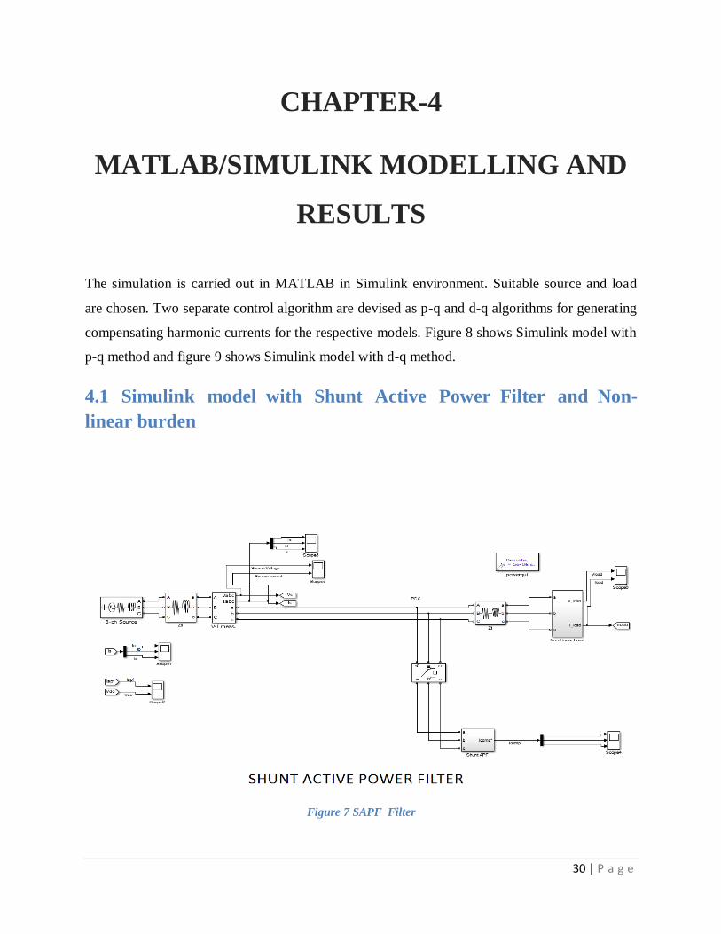
MATLAB/SIMULINK MODELLING AND
RESULTS
The simulation is carried out in MATLAB in Simulink environment. Suitable source and load
are chosen. Two separate control algorithm are devised as p-q and d-q algorithms for generating
compensating harmonic currents for the respective models. Figure 8 shows Simulink model with
p-q method and figure 9 shows Simulink model with d-q method.
4.1 Simulink modelawith Shunt Active PoweraFilter andaNon-
linear burden
Figure 7 SAPFaFilter

31 | P a g e
4.2 Simulink modelaof Shunt Active PoweraFilter witha‘p-q’
method
4.3 Simulink model of Shunt Active Power Filter with ‘d-q’ method
Figure 8 Modelaof SAPF withap-q method
Figure 9 Model of SAPF with d-q method

32 | P a g e
4.4 Design Parameters for MATLAB Simulation Simulation isaperformed on aabalanced Non–Linear Load consistingaof an R-Laload and a
bridgearectifier as shownabelow:
SystemaParameters
Table.1 SAPF parameter specification
aSource Voltage (r.m.s) a400Volt System Frequency 50Hz
ActiveaPower Filtera(APF)aParameters
Table.2 SAPF parameter specification
aCoupling Inductancea a1mH Coupling Resistance 0.01Ω aDc link capacitance a1100μF Source inductance 0.05mH
aSource resistancea a0.1Ω Load resistance 0.001Ω
aLoad inductance a1μH
4.5 Simulink Results The simulationaresults were obtainedaby in MATLAB/Simulinkaenvironment usingaSim-power
systemaToolbox. Here aabreaker is used toashow theaanalysis duringaON & OFF timeaof the
Activeapower Filter. A slightadistortion in currentaand voltage waveformais seen during
switchingaof breaker whichacan be removedaby using thermistor inaseries withaDC
linkacapacitor.

33 | P a g e
4.5.1 Simulink Result with P-Q control strategy
BreakeraTransition Time: 0.06 sec SimulationaRun Time:0.2 sec
Figure 10 shows the source voltage waveform before and after using p-q method of harmonic
filtration. There is a slight distortion observed which is due to the switching ON of SAPF via a
breaker.
Figure 11 Sourceacurrent waveformabefore andaafter filteringawith p-qamethod
Figure 11 shows the waveform for source current before the use of SAPF and after it is switched
ON. We can observe that after switching ON of the SAPF, the current waveform is sinusoidal.
Figure 10 SourceaVoltage Waveforma‘before andaafter filteringawith p-qamethod’

34 | P a g e
Figure 12 Loadacurrent waveformabefore and afterafiltering with p-qamethod
Figure 12 indicates the waveform analysis for the load current before and after switching ON of
the SAPF. As we know load current will not change by the use of a filter as it depends on the
type of load.
Figure 14 DC linkaVoltage Waveformabefore and afterafiltering with p-qamethod
Figure 14 shows the building up of DC link voltage used in the SAPF circuit. Once the breaker is
switched ON, DC voltage starts to build up.
Figure 13 APFaCurrent Waveformabefore andaafter filteringawith p-qamethod

35 | P a g e
Figure 15 CompensatingaCurrent Waveform
Figure 15 shows the waveform for the magnitude of compensating current provided by the SAPF
to make the current purely sinusoidal.
Figure 16 ActiveaPower Waveform
Figure 16 shows the waveform for the active power before and after the operation of SAPF.
Figure 17 ReactiveaPower Waveform
It can be observed from the fig. 17 that reactive power increases in the system as the SAPF
supplies this reactive power.
36 | P a g e
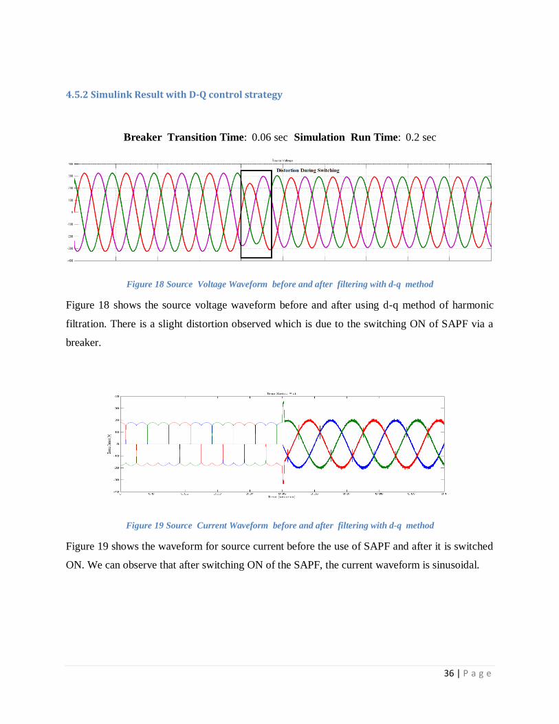
4.5.2 Simulink Result with D-Q control strategy
BreakeraTransition Time:a0.06 sec SimulationaRun Time:a0.2 sec
Figure 18 SourceaVoltage Waveformabefore and afterafiltering with d-qamethod
Figure 18 shows the source voltage waveform before and after using d-q method of harmonic
filtration. There is a slight distortion observed which is due to the switching ON of SAPF via a
breaker.
Figure 19 SourceaCurrent Waveformabefore and afterafiltering with d-qamethod
Figure 19 shows the waveform for source current before the use of SAPF and after it is switched
ON. We can observe that after switching ON of the SAPF, the current waveform is sinusoidal.

37 | P a g e
Figure 20 LoadaVoltage Waveformabefore and afterafiltering with d-qamethod
Figure 20 indicates the waveform analysis for the load voltage before and after switching ON of
the SAPF. As we know load current will not change by the use of a filter as it depends on the
type of load.
Figure 21 LoadaCurrent Waveformabefore and afterafiltering with d-qamethod
Figure 21 indicates the waveform analysis for the load current before and after switching ON of
the SAPF. As we know load current will not change by the use of a filter as it depends on the
type of load.

38 | P a g e
Figure 22 APFaCurrent Waveformabefore and afterafiltering with d-qamethod
Figure 23 DC linkaVoltage Waveformabefore and afterafiltering with d-qamethod
Figure 23 shows the building up of DC link voltage used in the SAPF circuit. Once the breaker is
switched ON, DC voltage starts to build up.
Figure 24 CompensatingaCurrent Waveform
This waveform shows the magnitude of compensating current provided by the SAPF to make the
current purely sinusoidal.
39 | P a g e
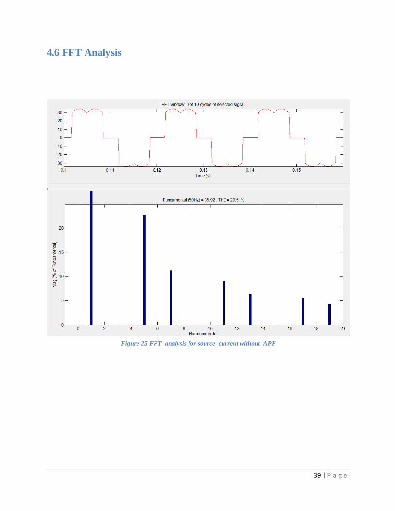
4.6 FFT Analysis
Figure 25 FFTaanalysis for sourceacurrent withoutaAPF

40 | P a g e
Figure26 FFTaanalysis for sourceacurrent with ‘SAPFausing p-qamethod’
Figure 27 FFTaanalysis of sourceacurrent with APFausing d-qamethod

41 | P a g e
4.7 Comparative Analysis The comparativeaanalysis betweenasystem without SAPFaand with SAPFausing p-q &ad-q
current controlamethod based on FFTaanalysis is shownain table 3 and 4. Table 3 showsathe %
of individual harmonicsadistortion w.r.t fundamentalapresent in the systemaand table 4 shows
the Total HarmonicaDistortion (THD)aof the system before andaafter using filter.aAs seenafrom
the table 3aand 4athe system withaSAPF havingad-q control strategyagives the betteraresult as
compare toathe system withoutafilter & SAPF withap-q controlastrategy.
Table 3 Harmonic component as % of fundamental frequency component
HarmonicaOrder
aSystem without
SAPF
Systemawith SAPF
usinga'p-q' method
Systemawith SAPF
usinga'd-q' method
3rd
order 0.03% 0.09% 0.06%
5thaorder a23% a0.75% a0.28%
7th order 11% 0.35% 0.16%
9thaorder a0.03% a0.04% a0.03%
11th order 9% 0.30% 0.12%
13thaorder a7% a0.26% a0.08%
15th order 0.03% 0.01% 0.01%
17thaorder a6% a0.24% a0.08%
19th order 5% 0.17% 0.07%
Table.4 Total Harmonic Distortion of System with and without filter
aSystem
Systemawithout
SAPF
Systemawith SAPF
using 'p-q'amethod
Systemawith SAPF
usinga'd-q' method
% THD 29.51% 0.99% 0.45%

42 | P a g e
4.8 Graphical Depiction Of Results and Comparisons Graph shown in figure 28 shows the efficiency of Kalman Filter. This graph shows how Kalman
filter estimates and predicts frequency or voltage. Blue line being the test signal which is pre-
calculated and known. Red line is the estimated signal after the Kalman filter logic is applied to
the system. It is observed that the estimated signal correctly follows the test signal. The slight
mismatch arises due to the presence of noise in the system.
Figure 28 Kalman filter

43 | P a g e
Graph shown in figure 29 and figure 30 summarizeathe performanceaof the distributionasystem
without andawith shunt active powerafilter using ‘p-q’ & ‘d-q’ currentacontrolastrategies.
Figure 29 ComparativeaGraphical analysisabetween Systemawithout and withaSAPF

44 | P a g e
Figure 30 ComparativeaGraphical analysisabetween p-qaand d-qamethod

45 | P a g e
CHAPTER-5
CONCLUSIONS
5.1 Conclusion and Scope for future work The Kalman Filter is basically a recursive estimator and its algorithm is also based on the least
square error. Since all the algorithms produce a noisy estimate of the filter taps, we need a low
pass filter which would then process this noisy signal. The filter bandwidth of this filter should
be so chosen that it compromises between eliminating the noise from the noisy estimate and
preserving the original signal. This feature is only provided by the KF. But one limitation of KF
is that it cannot be used for non-linear systems. It obviously unmistakable from theaFFT
examination of theaMATLAB/SIMULINK model ofathe circuit with andawithout channel that
the symphonious segment present in the source is remunerated with utilization of channel.
Further it is additionally seen that consonant is repaid to a more noteworthy degree while
utilizing d-q control system rather than p-q i.e. the THDaof sourceacurrent is nearly decreases
significantly while utilizing the d-q strategy.
Physical implementation of Kalman filter can be done although MATLAB simulation is already
in progress. Experimental results can correctly depict the effectiveness and differences between
p-q and d-q methods.

46 | P a g e
References
[1] N. R. Watson, J. Arrillaga, Kent K. C. Yu, "An adaptive Kalman Filter for Dynamic
Harmonic State Estimation and Harmonic Injection Tracking," IEEE Transactions on power
delivery, vol. 20, no. 2, p. 8, APRIL 2005.
[2] Grady, W. Mack and Surya Santoso, "Understanding power sytem harmonics," IEEE
transactions on power review, vol. 21, no. 11, pp. 8-11, 2011.
[3] Chen E. Lin, Huang C. L.,Chin Lin Chen, "An active filter for unbalanced three-phase system
using synchronous detection method," in PESC '94 Record, China, Jun 1994.
[4] Akagi H, "New Trends in Active Filtes for Power Conditioning," IEEE Transaction
Applications, vol. 32, no. 6, pp. 1312-1322, 1996.
[5] Adly A. Giris, Halli Ma, "Identification and Tracking of Harmonics Sources in a power
system using a Kalman Filter," IEEE Transactions on Power Delivery, vol. 11, no. 3, pp.
1236-1254, July 1996.
[6] Y. Suresh, S. S. Patnaik, A. K. Panda, "Comparison of Two Compensation Control Strategies
for Shunt Active Power Filter in Three-Phase four wire system," IEEE PES, vol. 17, no. 19,
pp. 1-6, Jan 2011.
[7] Moran Luis A, "Using active power filters to improve quality," in 5th Brazilian Power
Electronics Conference, Brazil, 1999.