Estimation and Inference of Heterogeneous Treatment

Effects using Random Forests∗

Stefan WagerDepartment of Statistics

Stanford Universityswager@stanford.edu

Susan AtheyGraduate School of Business

Stanford Universityathey@stanford.edu

July 11, 2017

Abstract

Many scientific and engineering challenges—ranging from personalized medicine tocustomized marketing recommendations—require an understanding of treatment effectheterogeneity. In this paper, we develop a non-parametric causal forest for estimat-ing heterogeneous treatment effects that extends Breiman’s widely used random for-est algorithm. In the potential outcomes framework with unconfoundedness, we showthat causal forests are pointwise consistent for the true treatment effect, and have anasymptotically Gaussian and centered sampling distribution. We also discuss a prac-tical method for constructing asymptotic confidence intervals for the true treatmenteffect that are centered at the causal forest estimates. Our theoretical results rely on ageneric Gaussian theory for a large family of random forest algorithms. To our knowl-edge, this is the first set of results that allows any type of random forest, includingclassification and regression forests, to be used for provably valid statistical inference.In experiments, we find causal forests to be substantially more powerful than classicalmethods based on nearest-neighbor matching, especially in the presence of irrelevantcovariates.

Keywords: Adaptive nearest neighbors matching; asymptotic normality; potentialoutcomes; unconfoundedness.

1 Introduction

In many applications, we want to use data to draw inferences about the causal effect of atreatment: Examples include medical studies about the effect of a drug on health outcomes,studies of the impact of advertising or marketing offers on consumer purchases, evaluationsof the effectiveness of government programs or public policies, and “A/B tests” (large-scalerandomized experiments) commonly used by technology firms to select algorithms for rankingsearch results or making recommendations. Historically, most datasets have been too smallto meaningfully explore heterogeneity of treatment effects beyond dividing the sample into

∗Part of the results developed in this paper were made available as an earlier technical report “AsymptoticTheory for Random Forests”, available at http://arxiv.org/abs/1405.0352.

1

arX

iv:1

510.

0434

2v4

[st

at.M

E]

10

Jul 2

017

a few subgroups. Recently, however, there has been an explosion of empirical settings whereit is potentially feasible to customize estimates for individuals.

An impediment to exploring heterogeneous treatment effects is the fear that researcherswill iteratively search for subgroups with high treatment levels, and then report only the re-sults for subgroups with extreme effects, thus highlighting heterogeneity that may be purelyspurious [Assmann et al., 2000, Cook et al., 2004]. For this reason, protocols for clinicaltrials must specify in advance which subgroups will be analyzed, and other disciplines suchas economics have instituted protocols for registering pre-analysis plans for randomized ex-periments or surveys. However, such procedural restrictions can make it difficult to discoverstrong but unexpected treatment effect heterogeneity. In this paper, we seek to addressthis challenge by developing a powerful, nonparametric method for heterogeneous treatmenteffect estimation that yields valid asymptotic confidence intervals for the true underlyingtreatment effect.

Classical approaches to nonparametric estimation of heterogeneous treatment effects in-clude nearest-neighbor matching, kernel methods, and series estimation; see, e.g., Crumpet al. [2008], Lee [2009], and Willke et al. [2012]. These methods perform well in applica-tions with a small number of covariates, but quickly break down as the number of covariatesincreases. In this paper, we explore the use of ideas from the machine learning literature toimprove the performance of these classical methods with many covariates. We focus on thefamily of random forest algorithms introduced by Breiman [2001a], which allow for flexiblemodeling of interactions in high dimensions by building a large number of regression treesand averaging their predictions. Random forests are related to kernels and nearest-neighbormethods in that they make predictions using a weighted average of “nearby” observations;however, random forests differ in that they have a data-driven way to determine which nearbyobservations receive more weight, something that is especially important in environmentswith many covariates or complex interactions among covariates.

Despite their widespread success at prediction and classification, there are importanthurdles that need to be cleared before random forests are directly useful to causal inference.Ideally, an estimator should be consistent with a well-understood asymptotic sampling dis-tribution, so that a researcher can use it to test hypotheses and establish confidence intervals.For example, when deciding to use a drug for an individual, we may wish to test the hypothe-sis that the expected benefit from the treatment is less than the treatment cost. Asymptoticnormality results are especially important in the causal inference setting, both because manypolicy applications require confidence intervals for decision-making, and because it can bedifficult to directly evaluate the model’s performance using, e.g., cross validation, when es-timating causal effects. Yet, the asymptotics of random forests have been largely left open,even in the standard regression or classification contexts.

This paper addresses these limitations, developing a forest-based method for treatmenteffect estimation that allows for a tractable asymptotic theory and valid statistical inference.Following Athey and Imbens [2016], our proposed forest is composed of causal trees thatestimate the effect of the treatment at the leaves of the trees; we thus refer to our algorithmas a causal forest.

In the interest of generality, we begin our theoretical analysis by developing the desiredconsistency and asymptotic normality results in the context of regression forests. We provethese results for a particular variant of regression forests that uses subsampling to generate avariety of different trees, while it relies on deeply grown trees that satisfy a condition we call“honesty” to reduce bias. An example of an honest tree is one where the tree is grown usingone subsample, while the predictions at the leaves of the tree are estimated using a different

2

subsample. We also show that the heuristically motivated infinitesimal jackknife for randomforests developed by Efron [2014] and Wager et al. [2014] is consistent for the asymptoticvariance of random forests in this setting. Our proof builds on classical ideas from Efron andStein [1981], Hajek [1968], and Hoeffding [1948], as well as the adaptive nearest neighborsinterpretation of random forests of Lin and Jeon [2006]. Given these general results, wenext show that our consistency and asymptotic normality results extend from the regressionsetting to estimating heterogeneous treatment effects in the potential outcomes frameworkwith unconfoundedness [Neyman, 1923, Rubin, 1974].

Although our main focus in this paper is causal inference, we note that there are a varietyof important applications of the asymptotic normality result in a pure prediction context.For example, Kleinberg et al. [2015] seek to improve the allocation of medicare fundingfor hip or knee replacement surgery by detecting patients who had been prescribed such asurgery, but were in fact likely to die of other causes before the surgery would have beenuseful to them. Here we need predictions for the probability that a given patient will survivefor more than, say, one year that come with rigorous confidence statements; our results arethe first that enable the use of random forests for this purpose.

Finally, we compare the performance of the causal forest algorithm against classical k-nearest neighbor matching using simulations, finding that the causal forest dominates interms of both bias and variance in a variety of settings, and that its advantage increaseswith the number of covariates. We also examine coverage rates of our confidence intervalsfor heterogeneous treatment effects.

1.1 Related Work

There has been a longstanding understanding in the machine learning literature that predic-tion methods such as random forests ought to be validated empirically [Breiman, 2001b]: ifthe goal is prediction, then we should hold out a test set, and the method will be consideredas good as its error rate is on this test set. However, there are fundamental challenges withapplying a test set approach in the setting of causal inference. In the widely used potentialoutcomes framework we use to formalize our results [Neyman, 1923, Rubin, 1974], a treat-ment effect is understood as a difference between two potential outcomes, e.g., would thepatient have died if they received the drug vs. if they didn’t receive it. Only one of thesepotential outcomes can ever be observed in practice, and so direct test-set evaluation is ingeneral impossible.1 Thus, when evaluating estimators of causal effects, asymptotic theoryplays a much more important role than in the standard prediction context.

From a technical point of view, the main contribution of this paper is an asymptotic nor-mality theory enabling us to do statistical inference using random forest predictions. Recentresults by Biau [2012], Meinshausen [2006], Mentch and Hooker [2016], Scornet et al. [2015],and others have established asymptotic properties of particular variants and simplificationsof the random forest algorithm. To our knowledge, however, we provide the first set of con-ditions under which predictions made by random forests are both asymptotically unbiasedand Gaussian, thus allowing for classical statistical inference; the extension to the causalforests proposed in this paper is also new. We review the existing theoretical literature onrandom forests in more detail in Section 3.1.

1Athey and Imbens [2016] have proposed indirect approaches to mimic test-set evaluation for causalinference. However, these approaches require an estimate of the true treatment effects and/or treatmentpropensities for all the observations in the test set, which creates a new set of challenges. In the absence ofan observable ground truth in a test set, statistical theory plays a more central role in evaluating the noisein estimates of causal effects.

3

A small but growing literature, including Green and Kern [2012], Hill [2011] and Hill andSu [2013], has considered the use of forest-based algorithms for estimating heterogeneoustreatment effects. These papers use the Bayesian Additive Regression Tree (BART) methodof Chipman et al. [2010], and report posterior credible intervals obtained by Markov-chainMonte Carlo (MCMC) sampling based on a convenience prior. Meanwhile, Foster et al.[2011] use regression forests to estimate the effect of covariates on outcomes in treated andcontrol groups separately, and then take the difference in predictions as data and projecttreatment effects onto units’ attributes using regression or classification trees (in contrast, wemodify the standard random forest algorithm to focus on directly estimating heterogeneityin causal effects). A limitation of this line of work is that, until now, it has lacked formalstatistical inference results.

We view our contribution as complementary to this literature, by showing that forest-based methods need not only be viewed as black-box heuristics, and can instead be usedfor rigorous asymptotic analysis. We believe that the theoretical tools developed here willbe useful beyond the specific class of algorithms studied in our paper. In particular, ourtools allow for a fairly direct analysis of variants of the method of Foster et al. [2011].Using BART for rigorous statistical analysis may prove more challenging since, althoughBART is often successful in practice, there are currently no results guaranteeing posteriorconcentration around the true conditional mean function, or convergence of the MCMCsampler in polynomial time. Advances of this type would be of considerable interest.

Several papers use tree-based methods for estimating heterogeneous treatment effects. Ingrowing trees to build our forest, we follow most closely the approach of Athey and Imbens[2016], who propose honest, causal trees, and obtain valid confidence intervals for averagetreatment effects for each of the subpopulations (leaves) identified by the algorithm. (Insteadof personalizing predictions for each individual, this approach only provides treatment effectestimates for leaf-wise subgroups whose size must grow to infinity.) Other related approachesinclude those of Su et al. [2009] and Zeileis et al. [2008], which build a tree for treatmenteffects in subgroups and use statistical tests to determine splits; however, these papers donot analyze bias or consistency properties.

Finally, we note a growing literature on estimating heterogeneous treatment effects usingdifferent machine learning methods. Imai and Ratkovic [2013], Signorovitch [2007], Tianet al. [2014] and Weisberg and Pontes [2015] develop lasso-like methods for causal inferencein a sparse high-dimensional linear setting. Beygelzimer and Langford [2009], Dudık et al.[2011], and others discuss procedures for transforming outcomes that enable off-the-shelf lossminimization methods to be used for optimal treatment policy estimation. In the econo-metrics literature, Bhattacharya and Dupas [2012], Dehejia [2005], Hirano and Porter [2009],Manski [2004] estimate parametric or semi-parametric models for optimal policies, relying onregularization for covariate selection in the case of Bhattacharya and Dupas [2012]. Taddyet al. [2016] use Bayesian nonparametric methods with Dirichlet priors to flexibly estimatethe data-generating process, and then project the estimates of heterogeneous treatment ef-fects down onto the feature space using regularization methods or regression trees to getlow-dimensional summaries of the heterogeneity; but again, there are no guarantees aboutasymptotic properties.

4

2 Causal Forests

2.1 Treatment Estimation with Unconfoundedness

Suppose we have access to n independent and identically distributed training exampleslabeled i = 1, ..., n, each of which consists of a feature vector Xi ∈ [0, 1]d, a responseYi ∈ R, and a treatment indicator Wi ∈ 0, 1. Following the potential outcomes frameworkof Neyman [1923] and Rubin [1974] (see Imbens and Rubin [2015] for a review), we thenposit the existence of potential outcomes Y

(1)i and Y

(0)i corresponding respectively to the

response the i-th subject would have experienced with and without the treatment, and definethe treatment effect at x as

τ (x) = E[Y

(1)i − Y (0)

i

∣∣Xi = x]. (1)

Our goal is to estimate this function τ(x). The main difficulty is that we can only everobserve one of the two potential outcomes Y

(0)i , Y

(1)i for a given training example, and so

cannot directly train machine learning methods on differences of the form Y(1)i − Y (0)

i .In general, we cannot estimate τ(x) simply from the observed data (Xi, Yi, Wi) without

further restrictions on the data generating distribution. A standard way to make progressis to assume unconfoundedness [Rosenbaum and Rubin, 1983], i.e., that the treatment as-signment Wi is independent of the potential outcomes for Yi conditional on Xi:

Y(0)i , Y

(1)i

⊥⊥ Wi

∣∣ Xi. (2)

The motivation behind unconfoundedness is that, given continuity assumptions, it effectivelyimplies that we can treat nearby observations in x-space as having come from a randomizedexperiment; thus, nearest-neighbor matching and other local methods will in general beconsistent for τ(x).

An immediate consequence of unconfoundedness is that

E[Yi

(Wi

e (x)− 1−Wi

1− e (x)

) ∣∣Xi = x

]= τ (x) , where e (x) = E

[Wi

∣∣Xi = x]

(3)

is the propensity of receiving treatment at x. Thus, if we knew e(x), we would have accessto a simple unbiased estimator for τ(x); this observation lies at the heart of methods basedon propensity weighting [e.g., Hirano et al., 2003]. Many early applications of machinelearning to causal inference effectively reduce to estimating e(x) using, e.g., boosting, aneural network, or even random forests, and then transforming this into an estimate forτ(x) using (3) [e.g., McCaffrey et al., 2004, Westreich et al., 2010]. In this paper, we take amore indirect approach: We show that, under regularity assumptions, causal forests can usethe unconfoundedness assumption (2) to achieve consistency without needing to explicitlyestimate the propensity e(x).

2.2 From Regression Trees to Causal Trees and Forests

At a high level, trees and forests can be thought of as nearest neighbor methods with anadaptive neighborhood metric. Given a test point x, classical methods such as k-nearestneighbors seek the k closest points to x according to some pre-specified distance measure,e.g., Euclidean distance. In contrast, tree-based methods also seek to find training examplesthat are close to x, but now closeness is defined with respect to a decision tree, and the

5

closest points to x are those that fall in the same leaf as it. The advantage of trees is thattheir leaves can be narrower along the directions where the signal is changing fast and wideralong the other directions, potentially leading a to a substantial increase in power when thedimension of the feature space is even moderately large.

In this section, we seek to build causal trees that resemble their regression analogues asclosely as possible. Suppose first that we only observe independent samples (Xi, Yi), andwant to build a CART regression tree. We start by recursively splitting the feature spaceuntil we have partitioned it into a set of leaves L, each of which only contains a few trainingsamples. Then, given a test point x, we evaluate the prediction µ(x) by identifying the leafL(x) containing x and setting

µ (x) =1

|i : Xi ∈ L(x)|∑

i:Xi∈L(x)

Yi. (4)

Heuristically, this strategy is well-motivated if we believe the leaf L(x) to be small enoughthat the responses Yi inside the leaf are roughly identically distributed. There are severalprocedures for how to place the splits in the decision tree; see, e.g., Hastie et al. [2009].

In the context of causal trees, we analogously want to think of the leaves as small enoughthat the (Yi, Wi) pairs corresponding to the indices i for which i ∈ L(x) act as though theyhad come from a randomized experiment. Then, it is natural to estimate the treatmenteffect for any x ∈ L as

τ (x) =1

|i : Wi = 1, Xi ∈ L|∑

i:Wi=1, Xi∈L

Yi −1

|i : Wi = 0, Xi ∈ L|∑

i:Wi=0, Xi∈L

Yi. (5)

In the following sections, we will establish that such trees can be used to grow causal foreststhat are consistent for τ(x).2

Finally, given a procedure for generating a single causal tree, a causal forest generatesan ensemble of B such trees, each of which outputs an estimate τb(x). The forest thenaggregates their predictions by averaging them: τ(x) = B−1

∑Bb=1 τb(x). We always assume

that the individual causal trees in the forest are built using random subsamples of s trainingexamples, where s/n 1; for our theoretical results, we will assume that s nβ for someβ < 1. The advantage of a forest over a single tree is that it is not always clear whatthe “best” causal tree is. In this case, as shown by Breiman [2001a], it is often better togenerate many different decent-looking trees and average their predictions, instead of seekinga single highly-optimized tree. In practice, this aggregation scheme helps reduce varianceand smooths sharp decision boundaries [Buhlmann and Yu, 2002].

2.3 Asymptotic Inference with Causal Forests

Our results require some conditions on the forest-growing scheme: The trees used to buildthe forest must be grown on subsamples of the training data, and the splitting rule must

2The causal tree algorithm presented above is a simplification of the method of Athey and Imbens [2016].The main difference between our approach and that of Athey and Imbens [2016] is that they seek to build asingle well-tuned tree; to this end, they use fairly large leaves and apply a form propensity weighting basedon (3) within each leaf to correct for variations in e(x) inside the leaf. In contrast, we follow Breiman [2001a]and build our causal forest using deep trees. Since our leaves are small, we are not required to apply anyadditional corrections inside them. However, if reliable propensity estimates are available, using them asweights for our method may improve performance (and would not conflict with the theoretical results).

6

not “inappropriately” incorporate information about the outcomes Yi as discussed formallyin Section 2.4. However, given these high level conditions, we obtain a widely applicableconsistency result that applies to several different interesting causal forest algorithms.

Our first result is that causal forests are consistent for the true treatment effect τ(x).To achieve pointwise consistency, we need to assume that the conditional mean functionsE[Y (0)

∣∣X = x]

and E[Y (1)

∣∣X = x]

are both Lipschitz continuous. To our knowledge, allexisting results on pointwise consistency of regression forests [e.g., Biau, 2012, Meinshausen,2006] require an analogous condition on E

[Y∣∣X = x

]. This is not particularly surprising,

as forests generally have smooth response surfaces [Buhlmann and Yu, 2002]. In addition tocontinuity assumptions, we also need to assume that we have overlap, i.e., for some ε > 0and all x ∈ [0, 1]d,

ε < P[W = 1

∣∣X = x]< 1− ε. (6)

This condition effectively guarantees that, for large enough n, there will be enough treatmentand control units near any test point x for local methods to work.

Beyond consistency, in order to do statistical inference on the basis of the estimatedtreatment effects τ(x), we need to understand their asymptotic sampling distribution. Usingthe potential nearest neighbors construction of Lin and Jeon [2006] and classical analysistools going back to Hoeffding [1948] and Hajek [1968], we show that—provided the sub-sample size s scales appropriately with n—the predictions made by a causal forest areasymptotically Gaussian and unbiased. Specifically, we show that

(τ (x)− τ (x))/√

Var [τ(x)]⇒ N (0, 1) (7)

under the conditions required for consistency, provided the subsample size s scales as s nβfor some βmin < β < 1

Moreover, we show that the asymptotic variance of causal forests can be accuratelyestimated. To do so, we use the infinitesimal jackknife for random forests developed byEfron [2014] and Wager et al. [2014], based on the original infinitesimal jackknife procedureof Jaeckel [1972]. This method assumes that we have taken the number of trees B to be largeenough that the Monte Carlo variability of the forest does not matter; and only measuresthe randomness in τ(x) due to the training sample.

To define the variance estimates, let τ∗b (x) be the treatment effect estimate given by theb-th tree, and let N∗ib ∈ 0, 1 indicate whether or not the i-th training example was usedfor the b-th tree.3 Then, we set

VIJ (x) =n− 1

n

(n

n− s

)2 n∑i=1

Cov∗ [τ∗b (x) , N∗ib]2, (8)

where the covariance is taken with respect to the set of all the trees b = 1, .., B used inthe forest. The term n(n − 1)/(n − s)2 is a finite-sample correction for forests grown bysubsampling without replacement; see Proposition 10. We show that this variance estimateis consistent, in the sense that VIJ (x) /Var [τ(x)]→p 1.

2.4 Honest Trees and Forests

In our discussion so far, we have emphasized the flexible nature of our results: for a widevariety of causal forests that can be tailored to the application area, we achieve both con-sistency and centered asymptotic normality, provided the sub-sample size s scales at an

3For double-sample trees defined in Procedure 1, N∗ib = 1 if the i-th example appears in either the

I-sample or the J -sample.

7

appropriate rate. Our results do, however, require the individual trees to satisfy a fairlystrong condition, which we call honesty: a tree is honest if, for each training example i, itonly uses the response Yi to estimate the within-leaf treatment effect τ using (5) or to decidewhere to place the splits, but not both. We discuss two causal forest algorithms that satisfythis condition.

Our first algorithm, which we call a double-sample tree, achieves honesty by dividingits training subsample into two halves I and J . Then, it uses the J -sample to place thesplits, while holding out the I-sample to do within-leaf estimation; see Procedure 1 fordetails. In our experiments, we set the minimum leaf size to k = 1. A similar family ofalgorithms was discussed in detail by Denil et al. [2014], who showed that such forests couldachieve competitive performance relative to standard tree algorithms that do not divide theirtraining samples. In the semiparametric inference literature, related ideas go back at leastto the work of Schick [1986].

We note that sample splitting procedures are sometimes criticized as inefficient becausethey “waste” half of the training data at each step of the estimation procedure. However, inour case, the forest subampling mechanism enables us to achieve honesty without wasting anydata in this sense, because we re-randomize the I/J -data splits over each subsample. Thus,although no data point can be used for split selection and leaf estimation in a single tree,each data point will participate in both I and J samples of some trees, and so will be usedfor both specifying the structure and treatment effect estimates of the forest. Although ouroriginal motivation for considering double-sample trees was to eliminate bias and thus enablecentered confidence intervals, we find that in practice, double-sample trees can improve uponstandard random forests in terms of mean-squared error as well.

Another way to build honest trees is to ignore the outcome data Yi when placing splits,and instead first train a classification tree for the treatment assignments Wi (Procedure 2).Such propensity trees can be particularly useful in observational studies, where we want tominimize bias due to variation in e(x). Seeking estimators that match training examplesbased on estimated propensity is a longstanding idea in causal inference, going back toRosenbaum and Rubin [1983].

Remark 1. For completeness, we briefly outline the motivation for the splitting rule ofAthey and Imbens [2016] we use for our double-sample trees. This method is motivated byan algorithm for minimizing the squared-error loss in regression trees. Because regressiontrees compute predictions µ by averaging training responses over leaves, we can verify that∑

i∈J(µ (Xi)− Yi)2

=∑i∈J

Y 2i −

∑i∈J

µ (Xi)2. (9)

Thus, finding the squared-error minimizing split is equivalent to maximizing the variance ofµ(Xi) for i ∈ J ; note that

∑i∈J µ(Xi) =

∑i∈J Yi for all trees, and so maximizing variance

is equivalent to maximizing the sum of the µ(Xi)2. In Procedure 1, we emulate this algorithm

by picking splits that maximize the variance of τ(Xi) for i ∈ J .4

Remark 2. In Appendix B, we present evidence that adaptive forests with small leavescan overfit to outliers in ways that make them inconsistent near the edges of sample space.Thus, the forests of Breiman [2001a] need to be modified in some way to get pointwise

4Athey and Imbens [2016] also consider “honest splitting rules” that anticipate honest estimation, andcorrect for the additional sampling variance in small leaves using an idea closely related to the Cp penalty ofMallows [1973]. Although it could be of interest for further work, we do not study the effect of such splittingrules here.

8

Procedure 1. Double-Sample Trees

Double-sample trees split the available training data into two parts: one half for esti-mating the desired response inside each leaf, and another half for placing splits.

Input: n training examples of the form (Xi, Yi) for regression trees or (Xi, Yi, Wi)for causal trees, where Xi are features, Yi is the response, and Wi is the treatmentassignment. A minimum leaf size k.

1. Draw a random subsample of size s from 1, ..., n without replacement, and thendivide it into two disjoint sets of size |I| = bs/2c and |J | = ds/2e.

2. Grow a tree via recursive partitioning. The splits are chosen using any data fromthe J sample and X- or W -observations from the I sample, but without usingY -observations from the I-sample.

3. Estimate leaf-wise responses using only the I-sample observations.

Double-sample regression trees make predictions µ(x) using (4) on the leaf containing x,only using the I-sample observations. The splitting criteria is the standard for CARTregression trees (minimizing mean-squared error of predictions). Splits are restricted sothat each leaf of the tree must contain k or more I-sample observations.

Double-sample causal trees are defined similarly, except that for prediction we estimateτ(x) using (5) on the I sample. Following Athey and Imbens [2016], the splits of thetree are chosen by maximizing the variance of τ(Xi) for i ∈ J ; see Remark 1 for details.In addition, each leaf of the tree must contain k or more I-sample observations of eachtreatment class.

consistency results; here, we use honesty following, e.g., Wasserman and Roeder [2009].We note that there have been some recent theoretical investigations of non-honest forests,including Scornet et al. [2015] and Wager and Walther [2015]. However, Scornet et al. [2015]do not consider pointwise properties of forests; whereas Wager and Walther [2015] showconsistency of adaptive forests with larger leaves, but their bias bounds decay slower thanthe sampling variance of the forests and so cannot be used to establish centered asymptoticnormality.

3 Asymptotic Theory for Random Forests

In order to use random forests to provide formally valid statistical inference, we need anasymptotic normality theory for random forests. In the interest of generality, we first de-velop such a theory in the context of classical regression forests, as originally introduced byBreiman [2001a]. In this section, we assume that we have training examples Zi = (Xi, Yi)for i = 1, ..., n, a test point x, and we want to estimate true conditional mean function

µ (x) = E[Y∣∣X = x

]. (10)

9

Procedure 2. Propensity Trees

Propensity trees use only the treatment assignment indicator Wi to place splits, andsave the responses Yi for estimating τ .

Input: n training examples (Xi, Yi, Wi), where Xi are features, Yi is the response, andWi is the treatment assignment. A minimum leaf size k.

1. Draw a random subsample I ∈ 1, ..., n of size |I| = s (no replacement).

2. Train a classification tree using sample I where the outcome is the treatmentassignment, i.e., on the (Xi, Wi) pairs with i ∈ I. Each leaf of the tree must havek or more observations of each treatment class.

3. Estimate τ(x) using (5) on the leaf containing x.

In step 2, the splits are chosen by optimizing, e.g., the Gini criterion used by CART forclassification [Breiman et al., 1984].

We also have access to a regression tree T which can be used to get estimates of the con-ditional mean function at x of the form T (x; ξ, Z1, ..., Zn), where ξ ∼ Ξ is a source ofauxiliary randomness. Our goal is to use this tree-growing scheme to build a random forestthat can be used for valid statistical inference about µ(x).

We begin by precisely describing how we aggregate individual trees into a forest. Forus, a random forest is an average of trees trained over all possible size-s subsamples of thetraining data, marginalizing over the auxiliary noise ξ. In practice, we compute such arandom forest by Monte Carlo averaging, and set

RF (x; Z1, ..., Zn) ≈ 1

B

B∑b=1

T (x; ξ∗b , Z∗b1, ..., Z

∗bs) , (11)

where Z∗b1, ..., Z∗bs is drawn without replacement from Z1, ..., Zn, ξ∗b is a random drawfrom Ξ, and B is the number of Monte Carlo replicates we can afford to perform. Theformulation (12) arises as the B →∞ limit of (11); thus, our theory effectively assumes thatB is large enough for Monte Carlo effects not to matter. The effects of using a finite B arestudied in detail by Mentch and Hooker [2016]; see also Wager et al. [2014], who recommendtaking B on the order of n.

Definition 1. The random forest with base learner T and subsample size s is

RF (x; Z1, ..., Zn) =

(n

s

)−1 ∑1≤i1<i2<...<is≤n

Eξ∼Ξ [T (x; ξ, Zi1 , ..., Zis)] . (12)

Next, as described in Section 2, we require that the trees T in our forest be honest.Double-sample trees, as defined in Procedure 1, can always be used to build honest trees withrespect to the I-sample. In the context of causal trees for observational studies, propensitytrees (Procedure 2) provide a simple recipe for building honest trees without sample splitting.

10

Definition 2. A tree grown on a training sample (Z1 = (X1, Y1) , ..., Zs = (Xs, Ys)) ishonest if (a) (standard case) the tree does not use the responses Y1, ..., Ys in choosing whereto place its splits; or (b) (double sample case) the tree does not use the I-sample responsesfor placing splits.

In order to guarantee consistency, we also need to enforce that the leaves of the treesbecome small in all dimensions of the feature space as n gets large.5 Here, we followMeinshausen [2006], and achieve this effect by enforcing some randomness in the way treeschoose the variables they split on: At each step, each variable is selected with probabilityat least π/d for some 0 < π ≤ 1 (for example, we could satisfy this condition by completelyrandomizing the splitting variable with probability π). Formally, the randomness in how topick the splitting features is contained in the auxiliary random variable ξ.

Definition 3. A tree is a random-split tree if at every step of the tree-growing procedure,marginalizing over ξ, the probability that the next split occurs along the j-th feature isbounded below by π/d for some 0 < π ≤ 1, for all j = 1, ..., d.

The remaining definitions are more technical. We use regularity to control the shape ofthe tree leaves, while symmetry is used to apply classical tools in establishing asymptoticnormality.

Definition 4. A tree predictor grown by recursive partitioning is α-regular for some α > 0if either (a) (standard case) each split leaves at least a fraction α of the available trainingexamples on each side of the split and, moreover, the trees are fully grown to depth k forsome k ∈ N, i.e., there are between k and 2k − 1 observations in each terminal node of thetree; or (b) (double sample case) if the predictor is a double-sample tree as in Procedure 1,the tree satisfies part (a) for the I sample.

Definition 5. A predictor is symmetric if the (possibly randomized) output of the predictordoes not depend on the order (i = 1, 2, ...) in which the training examples are indexed.

Finally, in the context of classification and regression forests, we estimate the asymptoticvariance of random forests using the original infinitesimal jackknife of Wager et al. [2014],i.e.,

VIJ (x) =n− 1

n

(n

n− s

)2 n∑i=1

Cov∗ [µ∗b (x) , N∗ib]2, (13)

where µ∗b(x) is the estimate for µ(x) given by a single regression tree. We note that thefinite-sample correction n(n − 1)/(n − s)2 did not appear in Wager et al. [2014], as theirpaper focused on subsampling with replacement, whereas this correction is only appropriatefor subsampling without replacement.

Given these preliminaries, we can state our main result on the asymptotic normality ofrandom forests. As discussed in Section 2.3, we require that the conditional mean functionµ (x) = E

[Y∣∣X = x

]be Lipschitz continuous. The asymptotic normality result requires

for the subsample size s to scale within the bounds given in (14). If the subsample sizegrows slower than this, the forest will still be asymptotically normal, but the forest may beasymptotically biased. For clarity, we state the following result with notation that makes

5Biau [2012] and Wager and Walther [2015] consider the estimation of low-dimensional signals embeddedin a high-dimensional ambient space using random forests; in this case, the variable selection properties oftrees also become important. We leave a study of asymptotic normality of random forests in high dimensionsto future work.

11

the dependence of µn(x) and sn on n explicit; in most of the paper, however, we drop thesubscripts to µn(x) and sn when there is no risk of confusion.

Theorem 1. Suppose that we have n independent and identically distributed trainingexamples Zi = (Xi, Yi) ∈ [0, 1]d × R. Suppose moreover that the features are inde-pendently and uniformly distributed 6 Xi ∼ U([0, 1]d), that µ(x) = E

[Y∣∣X = x

]and

µ2(x) = E[Y 2∣∣X = x

]are Lipschitz-continuous, and finally that Var

[Y∣∣X = x

]> 0

and E[|Y − E[Y∣∣X = x]|2+δ

∣∣X = x] ≤M for some constants δ, M > 0, uniformly over allx ∈ [0, 1]d. Given this data-generating process, let T be an honest, α-regular with α ≤ 0.2,and symmetric random-split tree in the sense of Definitions 2, 3, 4, and 5, and let µn(x) bethe estimate for µ(x) given by a random forest with base learner T and a subsample size sn.Finally, suppose that the subsample size sn scales as

sn nβ for some βmin := 1−

1 +d

π

log(α−1

)log(

(1− α)−1)−1

< β < 1. (14)

Then, random forest predictions are asymptotically Gaussian:

µn(x)− µ (x)

σn(x)⇒ N (0, 1) for a sequence σn(x)→ 0. (15)

Moreover, the asymptotic variance σn can be consistently estimated using the infinitesimaljackknife (8):

VIJ (x)/σ2n(x)→p 1. (16)

Remark 3 (binary classification). We note that Theorem 1 also holds for binary classifi-cation forests with leaf size k = 1, as is default in the R-package randomForest [Liaw andWiener, 2002]. Here, we treat the output RF(x) of the random forests as an estimate for theprobability P

[Y = 1

∣∣X = x]; Theorem 1 then lets us construct valid confidence intervals

for this probability. For classification forests with k > 1, the proof of Theorem 1 still holdsif the individual classification trees are built by averaging observations within a leaf, but notif they are built by voting. Extending our results to voting trees is left as further work.

The proof of this result is organized as follows. In Section 3.2, we provide bounds for thebias E [µn(x)− µ (x)] of random forests, while Section 3.3 studies the sampling distributionsof µn(x)− E [µn(x)] and establishes Gaussianity. Given a subsampling rate satisfying (14),the bias decays faster than the variance, thus allowing for (15). Before beginning the proof,however, we relate our result to existing results about random forests in Section 3.1.

3.1 Theoretical Background

There has been considerable work in understanding the theoretical properties of randomforests. The convergence and consistency properties of trees and random forests have beenstudied by, among others, Biau [2012], Biau et al. [2008], Breiman [2004], Breiman et al.[1984], Meinshausen [2006], Scornet et al. [2015], Wager and Walther [2015], and Zhu et al.[2015]. Meanwhile, their sampling variability has been analyzed by Duan [2011], Lin andJeon [2006], Mentch and Hooker [2016], Sexton and Laake [2009], and Wager et al. [2014].

6The result also holds with a density that is bounded away from 0 and infinity; however, we assumeuniformity for simpler exposition.

12

However, to our knowledge, our Theorem 1 is the first result establishing conditions underwhich predictions made by random forests are asymptotically unbiased and normal.

Probably the closest existing result is that of Mentch and Hooker [2016], who showedthat random forests based on subsampling are asymptotically normal under substantiallystronger conditions than us: they require that the subsample size s grows slower than

√n,

i.e., that sn/√n → 0. However, under these conditions, random forests will not in general

be asymptotically unbiased. As a simple example, suppose that d = 2, that µ(x) = ‖x‖1,and that we evaluate an honest random forest at x = 0. A quick calculation shows that thebias of the random forest decays as 1/

√sn, while its variance decays as sn/n. If sn/

√n→ 0,

the squared bias decays slower than the variance, and so confidence intervals built usingthe resulting Gaussian limit distribution will not cover µ(x). Thus, although the result ofMentch and Hooker [2016] may appear qualitatively similar to ours, it cannot be used forvalid asymptotic statistical inference about µ(x).

The variance estimator VIJ was studied in the context of random forests by Wager et al.[2014], who showed empirically that the method worked well for many problems of interest.Wager et al. [2014] also emphasized that, when using VIJ in practice, it is important toaccount for Monte Carlo bias. Our analysis provides theoretical backing to these results,by showing that VIJ is in fact a consistent estimate for the variance σ2

n(x) of random forestpredictions. The earlier work on this topic [Efron, 2014, Wager et al., 2014] had only mo-tivated the estimator VIJ by highlighting connections to classical statistical ideas, but didnot establish any formal justification for it.

Instead of using subsampling, Breiman originally described random forests in terms ofbootstrap sampling, or bagging [Breiman, 1996]. Random forests with bagging, however,have proven to be remarkably resistant to classical statistical analysis. As observed by Bujaand Stuetzle [2006], Chen and Hall [2003], Friedman and Hall [2007] and others, estimatorsof this form can exhibit surprising properties even in simple situations; meanwhile, usingsubsampling rather than bootstrap sampling has been found to avoid several pitfalls [e.g.,Politis et al., 1999]. Although they are less common in the literature, random forests basedon subsampling have also been occasionally studied and found to have good practical andtheoretical properties [e.g., Buhlmann and Yu, 2002, Mentch and Hooker, 2016, Scornetet al., 2015, Strobl et al., 2007].

Finally, an interesting question for further theoretical study is to understand the optimalscaling of the subsample size sn for minimizing the mean-squared error of random forests.For subsampled nearest-neighbors estimation, the optimal rate for sn is sn n1−(1+d/4)−1

[Biau et al., 2010, Samworth, 2012]. Here, our specific value for βmin depends on the upperbounds for bias developed in the following section. Now, as shown by Biau [2012], undersome sparsity assumptions on µ(x), it is possible to get substantially stronger bounds forthe bias of random forests; thus, it is plausible that under similar conditions we could pushback the lower bound βmin on the growth rate of the subsample size.

3.2 Bias and Honesty

We start by bounding the bias of regression trees. Our approach relies on showing that as thesample size s available to the tree gets large, its leaves get small; Lipschitz-continuity of theconditional mean function and honesty then let us bound the bias. In order to state a formalresult, define the diameter diam(L(x)) of a leaf L(x) as the length of the longest segmentcontained inside L(x), and similarly let diamj(L(x)) denote the length of the longest suchsegment that is parallel to the j-th axis. The following lemma is a refinement of a result of

13

Meinshausen [2006], who showed that diam(L(x))→p 0 for regular trees.

Lemma 2. Let T be a regular, random-split tree and let L(x) denote its leaf containing x.Suppose that X1, ..., Xs ∼ U

([0, 1]d

)independently. Then, for any 0 < η < 1, and for large

enough s,

P

diamj (L(x)) ≥(

s

2k − 1

)− 0.99 (1−η) log((1−α)−1)log(α−1)

πd

≤ ( s

2k − 1

)− η22 1

log(α−1)πd

.

This lemma then directly translates into a bound on the bias of a single regression tree.Since a forest is an average of independently-generated trees, the bias of the forest is thesame as the bias of a single tree.

Theorem 3. Under the conditions of Lemma 2, suppose moreover that µ (x) is Lipschitzcontinuous and that the trees T in the random forest are honest. Then, provided that α ≤ 0.2,the bias of the random forest at x is bounded by

|E [µ (x)]− µ (x)| = O

(s− 1

2

log((1−α)−1)log(α−1)

πd

);

the constant in the O-bound is given in the proof.

3.3 Asymptotic Normality of Random Forests

Our analysis of the asymptotic normality of random forests builds on ideas developed byHoeffding [1948] and Hajek [1968] for understanding classical statistical estimators such asU -statistics. We begin by briefly reviewing their results to give some context to our proof.Given a predictor T and independent training examples Z1, ..., Zn, the Hajek projection ofT is defined as

T = E [T ] +

n∑i=1

(E[T∣∣Zi]− E [T ]

). (17)

In other words, the Hajek projection of T captures the first-order effects in T . Classicalresults imply that Var

[T]≤ Var [T ], and further:

limn→∞

Var[T]/

Var [T ] = 1 implies that limn→∞

E[∥∥∥T − T∥∥∥2

2

]/Var [T ] = 0. (18)

Since the Hajek projection T is a sum of independent random variables, we should expect itto be asymptotically normal under weak conditions. Thus whenever the ratio of the varianceof T to that of T tends to 1, the theory of Hajek projections almost automatically guaranteesthat T will be asymptotically normal.7

If T is a regression tree, however, the condition from (18) does not apply, and we cannotuse the classical theory of Hajek projections directly. Our analysis is centered around aweaker form of this condition, which we call ν-incrementality. With our definition, predictorsT to which we can apply the argument (18) directly are 1-incremental.

7The moments defined in (17) depend on the data-generating process for the Zi, and so cannot beobserved in practice. Thus, the Hajek projection is mostly useful as an abstract theoretical tool. For areview of classical projection arguments, see Chapter 11 of Van der Vaart [2000].

14

Definition 6. The predictor T is ν(s)-incremental at x if

Var[T (x; Z1, ..., Zs)

]/Var [T (x; Z1, ..., Zs)] & ν(s),

where T is the Hajek projection of T (17). In our notation,

f(s) & g(s) means that lim infs→∞

f(s)/g(s) ≥ 1.

Our argument proceeds in two steps. First we establish lower bounds for the incremen-tality of regression trees in Section 3.3.1. Then, in Section 3.3.2 we show how we can turnweakly incremental predictors T into 1-incremental ensembles by subsampling (Lemma 7),thus bringing us back into the realm of classical theory. We also establish the consistency ofthe infinitesimal jackknife for random forests. Our analysis of regression trees is motivatedby the “potential nearest neighbors” model for random forests introduced by Lin and Jeon[2006]; the key technical device used in Section 3.3.2 is the ANOVA decomposition of Efronand Stein [1981]. The discussion of the infinitesimal jackknife for random forest builds onresults of Efron [2014] and Wager et al. [2014].

3.3.1 Regression Trees and Incremental Predictors

Analyzing specific greedy tree models such as CART trees can be challenging. We thusfollow the lead of Lin and Jeon [2006], and analyze a more general class of predictors—potential nearest neighbors predictors—that operate by doing a nearest-neighbor search overrectangles; see also Biau and Devroye [2010]. The study of potential (or layered) nearestneighbors goes back at least to Barndorff-Nielsen and Sobel [1966].

Definition 7. Consider a set of points X1, ..., Xs ∈ Rd and a fixed x ∈ Rd. A point Xi

is a potential nearest neighbor (PNN) of x if the smallest axis-aligned hyperrectangle withvertices x and Xi contains no other points Xj . Extending this notion, a PNN k-set of x is aset of points Λ ⊆ X1, ..., Xs of size k ≤ |L| < 2k−1 such that there exists an axis alignedhyperrectangle L containing x, Λ, and no other training points. A training example Xi iscalled a k-PNN of x if there exists a PNN k-set of x containing Xi. Finally, a predictor Tis a k-PNN predictor over Z if, given a training set

Z = (X1, Y1) , ..., (Xs, Ys) ∈Rd × Y

sand a test point x ∈ Rd, T always outputs the average of the responses Yi over a k-PNN setof x.

This formalism allows us to describe a wide variety of tree predictors. For example, asshown by Lin and Jeon [2006], any decision tree T that makes axis-aligned splits and hasleaves of size between k and 2k − 1 is a k-PNN predictor. In particular, the base learnersoriginally used by Breiman [2001a], namely CART trees grown up to a leaf size k [Breimanet al., 1984], are k-PNN predictors. Predictions made by k-PNN predictors can always bewritten as

T (x; ξ, Z1, ..., Zs) =

s∑i=1

SiYi, (19)

where Si is a selection variable that takes the value 1/|i : Xi ∈ L(x)| for indices i in theselected leaf-set L(x) and 0 for all other indices. If the tree is honest, we know in additionthat, for each i, Si is independent of Yi conditional on Xi.

15

An important property of k-PNN predictors is that we can often get a good idea aboutwhether Si is non-zero even if we only get to see Zi; more formally, as we show below,the quantity sVar

[E[S1

∣∣Z1

]]cannot get too small. Establishing this fact is a key step

in showing that k-PNNs are incremental. In the following result, T can be an arbitrarysymmetric k-PNN predictor.

Lemma 4. Suppose that the observations X1, X2, . . . are independent and identically dis-tributed on [0, 1]d with a density f that is bounded away from infinity, and let T be anysymmetric k-PNN predictor. Then, there is a constant Cf, d depending only on f and d suchthat, as s gets large,

sVar[E[S1

∣∣Z1

]]&

1

kCf, d

/log (s)

d, (20)

where Si is the indicator for whether the observation is selected in the subsample. When fis uniform over [0, 1]d, the bound holds with Cf, d = 2−(d+1) (d− 1)!.

When k = 1 we see that, marginally, S1 ∼ Bernoulli(1/s) and so sVar [S1] ∼ 1; moregenerally, a similar calculation shows that 1/(2k − 1) . sVar [S1] . 1/k. Thus, (20) canbe interpreted as a lower bound on how much information Z1 contains about the selectionevent S1.

Thanks to this result, we are now ready to show that all honest and regular random-splittrees are incremental. Notice that any symmetric k-regular tree following Definition 4 is alsoa symmetric k-PNN predictor.

Theorem 5. Suppose that the conditions of Lemma 4 hold and that T is an honest k-regularsymmetric tree in the sense of Definitions 2 (part a), 4 (part a), and 5. Suppose moreoverthat the conditional moments µ (x) and µ2(x) are both Lipschitz continuous at x. Finally,suppose that Var

[Y∣∣X = x

]> 0. Then T is ν (s)-incremental at x with

ν (s) = Cf, d/

log (s)d, (21)

where Cf, d is the constant from Lemma 4.

Finally, the result of Theorem 5 also holds for double-sample trees of the form describedin Procedure 1. To establish the following result, we note that a double-sample tree is anhonest, symmetric k-PNN predictor with respect to the I-sample, while all the data in theJ -sample can be folded into the auxiliary noise term ξ; the details are worked out in theproof.

Corollary 6. Under the conditions of Theorem 5, suppose that T is instead a double-sample tree (Procedure 1) satisfying Definitions 2 (part b), 4 (part b), and 5. Then, T is

ν-incremental, with ν (s) = Cf, d/(4 log (s)d).

3.3.2 Subsampling Incremental Base Learners

In the previous section, we showed that decision trees are ν-incremental, in that the Hajekprojection T of T preserves at least some of the variation of T . In this section, we show thatrandomly subsampling ν-incremental predictors makes them 1-incremental; this then lets usproceed with a classical statistical analysis. The following lemma, which flows directly fromthe ANOVA decomposition of Efron and Stein [1981], provides a first motivating result forour analysis.

16

Lemma 7. Let µ(x) be the estimate for µ(x) generated by a random forest with base learner

T as defined in (12), and let ˚µ be the Hajek projection of µ (17). Then

E[(µ (x)− ˚µ (x)

)2]≤( sn

)2

Var [T (x; ξ, Z1, ..., Zs)]

whenever the variance Var [T ] of the base learner is finite.

This technical result paired with Theorem 5 or Corollary 6 leads to an asymptotic Gaus-sianity result; from a technical point of view, it suffices to check Lyapunov-style conditionsfor the central limit theorem.

Theorem 8. Let µ(x) be a random forest estimator trained according the conditions ofTheorem 5 or Corollary 6. Suppose, moreover, that the subsample size sn satisfies

limn→∞

sn =∞ and limn→∞

sn log (n)d/n = 0,

and that E[|Y − E[Y∣∣X = x]|2+δ

∣∣X = x] ≤M for some constants δ, M > 0, uniformly overall x ∈ [0, 1]d. Then, there exists a sequence σn(x)→ 0 such that

µn (x)− E [µn (x)]

σn(x)⇒ N (0, 1) , (22)

where N (0, 1) is the standard normal distribution.

Moreover, as we show below, it is possible to accurately estimate the variance of a randomforest using the infinitesimal jackknife for random forests [Efron, 2014, Wager et al., 2014].

Theorem 9. Let VIJ (x; , Z1, ..., Zn) be the infinitesimal jackknife for random forests asdefined in (8). Then, under the conditions of Theorem 8,

VIJ (x; Z1, ..., Zn)/σ2n(x)→p 1. (23)

Finally, we end this section by motivating the finite sample correction n(n− 1)/(n− s)2

appearing in (13) by considering the simple case where we have trivial trees that do notmake any splits: T (x; ξ, Zi1 , ..., Zis) = s−1

∑sj=1 Yij . In this case, we can verify that the

full random forest is nothing but µ = n−1∑ni=1 Yi, and the standard variance estimator

Vsimple =1

n (n− 1)

n∑i=1

(Yi − Y

)2, Y =

1

n

n∑i=1

Yi

is well-known to be unbiased for Var [µ]. We show below that, for trivial trees VIJ = Vsimple,implying that our correction makes VIJ exactly unbiased in finite samples for trivial trees. Ofcourse, n(n−1)/(n− s)2 → 1, and so Theorem 9 would hold even without this finite-samplecorrection; however, we find it to substantially improve the performance of our method inpractice.

Proposition 10. For trivial trees T (x; ξ, Zi1 , ..., Zis) = s−1∑sj=1 Yij , the variance esti-

mate VIJ (13) is equivalent to the standard variance estimator Vsimple, and E[VIJ ] = Var [µ].

17

4 Inferring Heterogeneous Treatment Effects

We now return to our main topic, namely estimating heterogeneous treatment effects usingrandom forests in the potential outcomes framework with unconfoundedness, and adapt ourasymptotic theory for regression forests to the setting of causal inference. Here, we againwork with training data consisting of tuples Zi = (Xi, Yi, Wi) for i = 1, ..., n, where Xi

is a feature vector, Yi is the response, and Wi is the treatment assignment. Our goal isto estimate the conditional average treatment effect τ(x) = E

[Y (1) − Y (0)

∣∣X = x]

at apre-specified test point x. By analogy to Definition 1, we build our causal forest CF byaveraging estimates for τ obtained by training causal trees Γ over subsamples:

CF (x; Z1, ..., Zn) =

(n

s

)−1 ∑1≤i1<i2<...<is≤n

Eξ∼Ξ [Γ (x; ξ, Zi1 , ..., Zis)] . (24)

We seek an analogue to Theorem 1 for such causal forests.Most of the definitions used to state Theorem 1 apply directly to this context; however,

the notions of honesty and regularity need to be adapted slightly. Specifically, an honestcausal tree is not allowed to look at the responses Yi when making splits but can look at thetreatment assignments Wi. Meanwhile, a regular causal tree must have at least k examplesfrom both treatment classes in each leaf; in other words, regular causal trees seek to act asfully grown trees for the rare treatment assignment, while allowing for more instances of thecommon treatment assignment.

Definition 2b. A causal tree grown on a training sample (Z1 = (X1, Y1, W1), ...,Zs = (Xs, Ys, Ws)) is honest if (a) (standard case) the tree does not use the responsesY1, ..., Ys in choosing where to place its splits; or (b) (double sample case) the tree does notuse the I-sample responses for placing splits.

Definition 4b. A causal tree grown by recursive partitioning is α-regular at x for someα > 0 if either: (a) (standard case) (1) Each split leaves at least a fraction α of the availabletraining examples on each side of the split, (2) The leaf containing x has at least k observa-tions from each treatment group (Wi ∈ 0, 1) for some k ∈ N, and (3) The leaf containingx has either less than 2k − 1 observations with Wi = 0 or 2k − 1 observations with Wi = 1;or (b) (double-sample case) for a double-sample tree as defined in Procedure 1, (a) holds forthe I sample.

Given these assumptions, we show a close analogue to Theorem 1, given below. Themain difference relative to our first result about regression forests is that we now rely onunconfoundedness and overlap to achieve consistent estimation of τ(x). To see how theseassumptions enter the proof, recall that an honest causal tree uses the features Xi and thetreatment assignments Wi in choosing where to place its splits, but not the responses Yi.Writing I(1)(x) and I(0)(x) for the indices of the treatment and control units in the leafaround x, we then find that after the splitting stage

E[Γ (x)

∣∣X, W ] (25)

=

∑i∈I(1)(x) E

[Y (1)

∣∣X = Xi, W = 1]∣∣I(1)(x)

∣∣ −

∑i∈I(0)(x) E

[Y (0)

∣∣X = Xi, W = 0]∣∣I(0)(x)

∣∣=

∑i∈I(1)(x) E

[Y (1)

∣∣X = Xi

]∣∣I(1)(x)∣∣ −

∑i∈I(0)(x) E

[Y (0)

∣∣X = Xi

]∣∣I(0)(x)∣∣ ,

18

where the second equality follows by unconfoundedness (2). Thus, it suffices to show that thetwo above terms are consistent for estimating E

[Y (0)

∣∣X = x]

and E[Y (1)

∣∣X = x]. To do

so, we can essentially emulate the argument leading to Theorem 1, provided we can establishan analogue to Lemma 2 and give a fast enough decaying upper bound to the diameter ofL(x); this is where we need the overlap assumption. A proof of Theorem 11 is given in theappendix.

Theorem 11. Suppose that we have n independent and identically distributed training ex-amples Zi = (Xi, Yi, Wi) ∈ [0, 1]d × R × 0, 1. Suppose, moreover, that the treatmentassignment is unconfounded (2) and has overlap (6). Finally, suppose that both potentialoutcome distributions (Xi, Y

(0)i ) and (Xi, Y

(1)i ) satisfy the same regularity assumptions as

the pair (Xi, Yi) did in the statement of Theorem 1. Given this data-generating process, let Γbe an honest, α-regular with α ≤ 0.2, and symmetric random-split causal forest in the senseof Definitions 2b, 3, 4b, and 5, and let τ(x) be the estimate for τ(x) given by a causal forestwith base learner Γ and a subsample size sn scaling as in (14). Then, the predictions τ(x)are consistent and asymptotically both Gaussian and centered, and the variance of the causalforest can be consistently estimated using the infinitesimal jackknife for random forests, i.e.,(7) holds.

Remark 4. (testing at many points) We note that it is not in general possible to constructcausal trees that are regular in the sense of Definition 4b for all x simultaneously. As asimple example, consider the situation where d = 1, and Wi = 1 (Xi ≥ 0); then, the treecan have at most 1 leaf for which it is regular. In the proof of Theorem 11, we avoided thisissue by only considering a single test point x, as it is always possible to build a tree thatis regular at a single given point x. In practice, if we want to build a causal tree that canbe used to predict at many test points, we may need to assign different trees to be valid fordifferent test points. Then, when predicting at a specific x, we treat the set of trees thatwere assigned to be valid at that x as the relevant forest and apply Theorem 11 to it.

5 Simulation Experiments

In observational studies, accurate estimation of heterogeneous treatment effects requiresovercoming two potential sources of bias. First, we need to identify neighborhoods overwhich the actual treatment effect τ(x) is reasonably stable and, second, we need to makesure that we are not biased by varying sampling propensities e(x). The simulations hereaim to test the ability of causal forests to respond to both of these factors.

Since causal forests are adaptive nearest neighbor estimators, it is natural to use a non-adaptive nearest neighborhood method as our baseline. We compare our method to thestandard k nearest neighbors (k-NN) matching procedure, which estimates the treatmenteffect as

τKNN (x) =1

k

∑i∈S1(x)

Yi −1

k

∑i∈S0(x)

Yi, (26)

where S1 and S0 are the k nearest neighbors to x in the treatment (W = 1) and control(W = 0) samples respectively. We generate confidence intervals for the k-NN method bymodeling τKNN (x) as Gaussian with mean τ(x) and variance (V (S0) + V (S1))/(k (k − 1)),where V

(S0/1

)is the sample variance for S0/1.

The goal of this simulation study is to verify that forest-based methods can be used buildrigorous, asymptotically valid confidence intervals that improve over non-adaptive methods

19

like k-NN in finite samples. The fact that forest-based methods hold promise for treatmenteffect estimation in terms of predictive error has already been conclusively established else-where; for example, BART methods following Hill [2011] won the recent Causal InferenceData Analysis Challenge at the 2016 Atlantic Causal Inference Conference. We hope thatthe conceptual tools developed in this paper will prove to be helpful in analyzing a widevariety of forest-based methods.

5.1 Experimental Setup

We describe our experiments in terms of the sample size n, the ambient dimension d, as wellas the following functions:

main effect: m(x) = 2−1 E[Y (0) + Y (1)

∣∣X = x],

treatment effect: τ(x) = E[Y (1) − Y (0)

∣∣X = x],

treatment propensity: e(x) = P[W = 1

∣∣X = x].

In all our examples, we respect unconfoundedness (2), use X ∼ U([0, 1]d), and have ho-moscedastic noise Y (0/1) ∼ N

(E[Y (0/1)

∣∣X], 1). We evaluate performance in terms of ex-

pected mean-squared error for estimating τ(X) at a random test example X, as well asexpected coverage of τ(X) with a target coverage rate of 0.95.

In our first experiment, we held the treatment effect fixed at τ(x) = 0, and tested theability of our method to resist bias due to an interaction between e(x) and m(x). Thisexperiment is intended to emulate the problem that in observational studies, a treatmentassignment is often correlated with potential outcomes, creating bias unless the statisticalmethod accurately adjusts for covariates. k-NN matching is a popular approach for per-forming this adjustment in practice. Here, we set

e(X) =1

4(1 + β2, 4(X1)) , m(X) = 2X1 − 1, (27)

where βa, b is the β-density with shape parameters a and b. We used n = 500 samples andvaried d between 2 and 30. Since our goal is accurate propensity matching, we use propensitytrees (Procedure 2) as our base learner; we grew B = 1000 trees with s = 50.

For our second experiment, we evaluated the ability of causal forests to adapt to hetero-geneity in τ(x), while holding m(x) = 0 and e(x) = 0.5 fixed. Thanks to unconfoundedness,the fact that e(x) is constant means that we are in a randomized experiment. We set τ tobe a smooth function supported on the first two features:

τ (X) = ς (X1) ς (X2) , ς (x) = 1 +1

1 + e−20(x−1/3). (28)

We took n = 5000 samples, while varying the ambient dimension d from 2 to 8. For causalforests, we used double-sample trees with the splitting rule of Athey and Imbens [2016] asour base learner (Procedure 1). We used s = 2500 (i.e., |I| = 1250) and grew B = 2000trees.

One weakness of nearest neighbor approaches in general, and random forests in particular,is that they can fill the valleys and flatten the peaks of the true τ(x) function, especiallynear the edge of feature space. We demonstrate this effect using an example similar to the

20

mean-squared error coveraged CF 10-NN 100-NN CF 10-NN 100-NN2 0.02 (0) 0.21 (0) 0.09 (0) 0.95 (0) 0.93 (0) 0.62 (1)5 0.02 (0) 0.24 (0) 0.12 (0) 0.94 (1) 0.92 (0) 0.52 (1)

10 0.02 (0) 0.28 (0) 0.12 (0) 0.94 (1) 0.91 (0) 0.51 (1)15 0.02 (0) 0.31 (0) 0.13 (0) 0.91 (1) 0.90 (0) 0.48 (1)20 0.02 (0) 0.32 (0) 0.13 (0) 0.88 (1) 0.89 (0) 0.49 (1)30 0.02 (0) 0.33 (0) 0.13 (0) 0.85 (1) 0.89 (0) 0.48 (1)

Table 1: Comparison of the performance of a causal forests (CF) with that of the k-nearestneighbors (k-NN) estimator with k = 10, 100, on the setup (27). The numbers in parenthe-ses indicate the (rounded) standard sampling error for the last printed digit, obtained byaggregating performance over 500 simulation replications.

one studied above, except now τ(x) has a sharper spike in the x1, x2 ≈ 1 region:

τ (X) = ς (X1) ς (X2) , ς (x) =2

1 + e−12(x−1/2). (29)

We used the same training method as with (28), except with n = 10000, s = 2000, andB = 10000.

We implemented our simulations in R, using the packages causalTree [Athey and Imbens,2016] for building individual trees, randomForestCI [Wager et al., 2014] for computing VIJ ,and FNN [Beygelzimer et al., 2013] for k-NN regression. All our trees had a minimum leafsize of k = 1. Software replicating the above simulations is available from the authors.8

5.2 Results

In our first setup (27), causal forests present a striking improvement over k-NN matching;see Table 1. Causal forests succeed in maintaining a mean-squared error of 0.02 as d growsfrom 2 to 30, while 10-NN and 100-NN do an order of magnitude worse. We note thatthe noise of k-NN due to variance in Y after conditioning on X and W is already 2/k,implying that k-NN with k ≤ 100 cannot hope to match the performance of causal forests.Here, however, 100-NN is overwhelmed by bias, even with d = 2. Meanwhile, in terms ofuncertainty quantification, our method achieves nominal coverage up to d = 10, after whichthe performance of the confidence intervals starts to decay. The 10-NN method also achievesdecent coverage; however, its confidence intervals are much wider than ours as evidenced bythe mean-squared error.

Figure 1 offers some graphical diagnostics for causal forests in the setting of (27). Inthe left panel, we observe how the causal forest sampling variance σ2

n(x) goes to zero withn; while the center panel depicts the decay of the relative root-mean squared error of theinfinitesimal jackknife estimate of variance, i.e., E[(σ2

n(x)−σ2n(x))2]1/2/σ2

n(x). The boxplotsdisplay aggregate results for 1,000 randomly sampled test points x. Finally, the right-mostpanel evaluates the Gaussianity of the forest predictions. Here, we first drew 1,000 randomtest points x, and computed τ(x) using forests grown on many different training sets. Theplot shows standardized Gaussian QQ-plots aggregated over all these x; i.e., for each x, weplot Gaussian theoretical quantiles against sample quantiles of (τ(x)−E(τ(x)))/

√Var[τ(x)].

8The R package grf [Athey et al., 2016] provides a newer, high-performance implementation of causalforests, available on CRAN.

21

100 200 400 800 1600

0.00

0.02

0.04

0.06

n

fore

st s

ampl

ing

varia

nce

100 200 400 800 1600

0.0

0.5

1.0

1.5

n

inf.

jack

. rel

ativ

e rm

se

−2 −1 0 1 2

−2

−1

01

2

theoretical quantiles

sam

ple

quan

tiles

−2

−1

01

2

−2 −1 0 1 2

Causal forest variance Inf. jack. relative RMSE Prediction QQ-plot

Figure 1: Graphical diagnostics for causal forests in the setting of (27). The first twopanels evaluate the sampling error of causal forests and our infinitesimal jackknife estimateof variance over 1,000 randomly draw test points, with d = 20. The right-most panel showsstandardized Gaussian QQ-plots for predictions at the same 1000 test points, with n = 800and d = 20. The first two panels are computed over 50 randomly drawn training sets, andthe last one over 20 training sets.

mean-squared error coveraged CF 7-NN 50-NN CF 7-NN 50-NN2 0.04 (0) 0.29 (0) 0.04 (0) 0.97 (0) 0.93 (0) 0.94 (0)3 0.03 (0) 0.29 (0) 0.05 (0) 0.96 (0) 0.93 (0) 0.92 (0)4 0.03 (0) 0.30 (0) 0.08 (0) 0.94 (0) 0.93 (0) 0.86 (1)5 0.03 (0) 0.31 (0) 0.11 (0) 0.93 (1) 0.92 (0) 0.77 (1)6 0.02 (0) 0.34 (0) 0.15 (0) 0.93 (1) 0.91 (0) 0.68 (1)8 0.03 (0) 0.38 (0) 0.21 (0) 0.90 (1) 0.90 (0) 0.57 (1)

Table 2: Comparison of the performance of a causal forests (CF) with that of the k-nearestneighbors (k-NN) estimator with k = 7, 50, on the setup (28). The numbers in parenthe-ses indicate the (rounded) standard sampling error for the last printed digit, obtained byaggregating performance over 25 simulation replications.

In our second setup (28), causal forests present a similar improvement over k-NN match-ing when d > 2, as seen in Table 2.9 Unexpectedly, we find that the performance of causalforests improves with d, at least when d is small. To understand this phenomenon, we notethat the variance of a forest depends on the product of the variance of individual trees timesthe correlation between different trees [Breiman, 2001a, Hastie et al., 2009]. Apparently,when d is larger, the individual trees have more flexibility in how to place their splits, thusreducing their correlation and decreasing the variance of the full ensemble.

Finally, in the setting (29), Table 3 shows that causal forests still achieve an order ofmagnitude improvement over k-NN in terms of mean-squared error when d > 2, but strugglemore in terms of coverage. This appears to largely be a bias effect: especially as d gets larger,the random forest is dominated by bias instead of variance and so the confidence intervals

9When d = 2, we do not expect causal forests to have a particular advantage over k-NN since thetrue τ also has 2-dimensional support; our results mirror this, as causal forests appear to have comparableperformance to 50-NN.

22

mean-squared error coveraged CF 10-NN 100-NN CF 10-NN 100-NN2 0.02 (0) 0.20 (0) 0.02 (0) 0.94 (0) 0.93 (0) 0.94 (0)3 0.02 (0) 0.20 (0) 0.03 (0) 0.90 (0) 0.93 (0) 0.90 (0)4 0.02 (0) 0.21 (0) 0.06 (0) 0.84 (1) 0.93 (0) 0.78 (1)5 0.02 (0) 0.22 (0) 0.09 (0) 0.81 (1) 0.93 (0) 0.67 (0)6 0.02 (0) 0.24 (0) 0.15 (0) 0.79 (1) 0.92 (0) 0.58 (0)8 0.03 (0) 0.29 (0) 0.26 (0) 0.73 (1) 0.90 (0) 0.45 (0)

Table 3: Comparison of the performance of a causal forests (CF) with that of the k-nearestneighbors (k-NN) estimator with k = 10, 100, on the setup (29). The numbers in parenthe-ses indicate the (rounded) standard sampling error for the last printed digit, obtained byaggregating performance over 40 simulation replications.

d=

6

0.0 0.2 0.4 0.6 0.8 1.0

0.0

0.2

0.4

0.6

0.8

1.0

0.0 0.2 0.4 0.6 0.8 1.0

0.0

0.2

0.4

0.6

0.8

1.0

0.0 0.2 0.4 0.6 0.8 1.0

0.0

0.2

0.4

0.6

0.8

1.0

d=

20

0.0 0.2 0.4 0.6 0.8 1.0

0.0

0.2

0.4

0.6

0.8

1.0

0.0 0.2 0.4 0.6 0.8 1.0

0.0

0.2

0.4

0.6

0.8

1.0

0.0 0.2 0.4 0.6 0.8 1.0

0.0

0.2

0.4

0.6

0.8

1.0

True effect τ(x) Causal forest k∗-NN

Figure 2: The true treatment effect τ(Xi) at 10,000 random test examples Xi, along withestimates τ(Xi) produced by a causal forest and optimally-tuned k-NN, on data drawnaccording to (29) with d = 6, 20. The test points are plotted according to their first twocoordinates; the treatment effect is denoted by color, from dark (low) to light (high). Onthis simulation instance, causal forests and k∗-NN had a mean-squared error of 0.03 and0.13 respectively for d = 6, and of 0.05 and 0.62 respectively for d = 20. The optimal tuningchoices for k-NN were k∗ = 39 for d = 6, and k∗ = 24 for d = 20.

are not centered. Figure 2 illustrates this phenomenon: although the causal forest faithfullycaptures the qualitative aspects of the true τ -surface, it does not exactly match its shape,especially in the upper-right corner where τ is largest. Our theoretical results guarantee thatthis effect will go away as n → ∞. Figure 2 also helps us understand why k-NN performsso poorly in terms of mean-squared error: its predictive surface is both badly biased andnoticeably “grainy,” especially for d = 20. It suffers from bias not only at the boundary

23

where the treatment effect is largest, but also where the slope of the treatment effect is highin the interior.

These results highlight the promise of causal forests for accurate estimation of hetero-geneous treatment effects, all while emphasizing avenues for further work. An immediatechallenge is to control the bias of causal forests to achieve better coverage. Using morepowerful splitting rules is a good way to reduce bias by enabling the trees to focus moreclosely on the coordinates with the greatest signal. The study of splitting rules for treesdesigned to estimate causal effects is still in its infancy and improvements may be possible.

A limitation of the present simulation study is that we manually chose whether to usedouble-sample forests or propensity forests, depending on which procedure seemed moreappropriate in each problem setting. An important challenge for future work is to designsplitting rules that can automatically choose which characteristic of the training data tosplit on. A principled and automatic rule for choosing s would also be valuable.

We present additional simulation results in the supplementary material. Appendix A hasextensive simulations in the setting of Table 2 while varying both s and n; and also considersa simulation setting where the signal is spread out over many different features, meaningthat forests have less upside over baseline methods. Finally, in Appendix B, we study theeffect of honesty versus adaptivity on forest predictive error.

6 Discussion

This paper proposed a class of non-parametric methods for heterogeneous treatment effectestimation that allow for data-driven feature selection all while maintaining the benefitsof classical methods, i.e., asymptotically normal and unbiased point estimates with validconfidence intervals. Our causal forest estimator can be thought of as an adaptive nearestneighbor method, where the data determines which dimensions are most important to con-sider in selecting nearest neighbors. Such adaptivity seems essential for modern large-scaleapplications with many features.

In general, the challenge in using adaptive methods as the basis for valid statistical infer-ence is that selection bias can be difficult to quantify; see Berk et al. [2013], Chernozhukovet al. [2015], Taylor and Tibshirani [2015], and references therein for recent advances. In thispaper, pairing “honest” trees with the subsampling mechanism of random forests enabledus to accomplish this goal in a simple yet principled way. In our simulation experiments,our method provides dramatically better mean-squared error than classical methods whileachieving nominal coverage rates in moderate sample sizes.

A number of important extensions and refinements are left open. Our current results onlyprovide pointwise confidence intervals for τ(x); extending our theory to the setting of globalfunctional estimation seems like a promising avenue for further work. Another challenge isthat nearest-neighbor non-parametric estimators typically suffer from bias at the boundariesof the support of the feature space. A systematic approach to trimming at the boundaries,and possibly correcting for bias, would improve the coverage of the confidence intervals. Ingeneral, work can be done to identify methods that produce accurate variance estimates evenin more challenging circumstances, e.g., with small samples or a large number of covariates,or to identify when variance estimates are unlikely to be reliable.

24

Acknowledgment

We are grateful for helpful feedback from Brad Efron, Trevor Hastie, Guido Imbens, Guen-ther Walther, as well as the associate editor, two anonymous referees, and seminar partici-pants at Atlantic Causal Inference Conference, Berkeley Haas, Berkeley Statistics, CaliforniaEconometrics Conference, Cambridge, Carnegie Mellon, COMPSTAT, Cornell, ColumbiaBusiness School, Columbia Statistics, CREST, EPFL, ISAT/DARPA Machine Learning forCausal Inference, JSM, London Business School, Microsoft Conference on Digital Economics,Merck, MIT IDSS, MIT Sloan, Northwestern, SLDM, Stanford GSB, Stanford Statistics,University College London, University of Bonn, University of Chicago Booth, University ofChicago Statistics, University of Illinois Urbana–Champaign, University of Pennsylvania,University of Southern California, University of Washington, Yale Econometrics, and YaleStatistics. S. W. was partially supported by a B. C. and E. J. Eaves Stanford GraduateFellowship.

References

Susan F Assmann, Stuart J Pocock, Laura E Enos, and Linda E Kasten. Subgroup analysisand other (mis) uses of baseline data in clinical trials. The Lancet, 355(9209):1064–1069,2000.

Susan Athey and Guido Imbens. Recursive partitioning for heterogeneous causal effects.Proceedings of the National Academy of Sciences, 113(27):7353–7360, 2016.

Susan Athey, Julie Tibshirani, and Stefan Wager. Generalized random forests. arXiv preprintarXiv:1610.01271, 2016.

Ole Barndorff-Nielsen and Milton Sobel. On the distribution of the number of admissiblepoints in a vector random sample. Theory of Probability & Its Applications, 11(2):249–269,1966.

Richard Berk, Lawrence Brown, Andreas Buja, Kai Zhang, and Linda Zhao. Valid post-selection inference. The Annals of Statistics, 41(2):802–837, 2013.

Alina Beygelzimer and John Langford. The offset tree for learning with partial labels.In Proceedings of the 15th International Conference on Knowledge Discovery and DataMining, pages 129–138. ACM, 2009.

Alina Beygelzimer, Sham Kakadet, John Langford, Sunil Arya, David Mount, and ShengqiaoLi. FNN: Fast Nearest Neighbor Search Algorithms and Applications, 2013. URL http:

//CRAN.R-project.org/package=FNN. R package version 1.1.Debopam Bhattacharya and Pascaline Dupas. Inferring welfare maximizing treatment as-

signment under budget constraints. Journal of Econometrics, 167(1):168–196, 2012.Gerard Biau. Analysis of a random forests model. The Journal of Machine Learning Re-

search, 13:1063–1095, 2012.Gerard Biau and Luc Devroye. On the layered nearest neighbour estimate, the bagged

nearest neighbour estimate and the random forest method in regression and classification.Journal of Multivariate Analysis, 101(10):2499–2518, 2010.

Gerard Biau, Luc Devroye, and Gabor Lugosi. Consistency of random forests and otheraveraging classifiers. The Journal of Machine Learning Research, 9:2015–2033, 2008.

Gerard Biau, Frederic Cerou, and Arnaud Guyader. On the rate of convergence of the baggednearest neighbor estimate. The Journal of Machine Learning Research, 11:687–712, 2010.

Patrick Billingsley. Probability and Measure. John Wiley & Sons, 2008.

25

Leo Breiman. Bagging predictors. Machine Learning, 24(2):123–140, 1996.Leo Breiman. Random forests. Machine Learning, 45(1):5–32, 2001a.Leo Breiman. Statistical modeling: The two cultures (with comments and a rejoinder by

the author). Statistical Science, 16(3):199–231, 2001b.Leo Breiman. Consistency for a simple model of random forests. Statistical Department,

University of California at Berkeley. Technical Report, (670), 2004.Leo Breiman, Jerome Friedman, Charles J Stone, and Richard A Olshen. Classification and

Regression Trees. CRC press, 1984.Peter Buhlmann and Bin Yu. Analyzing bagging. The Annals of Statistics, 30(4):927–961,

2002.Andreas Buja and Werner Stuetzle. Observations on bagging. Statistica Sinica, 16(2):323,

2006.Song Xi Chen and Peter Hall. Effects of bagging and bias correction on estimators defined

by estimating equations. Statistica Sinica, 13(1):97–110, 2003.Victor Chernozhukov, Christian Hansen, and Martin Spindler. Valid post-selection and post-

regularization inference: An elementary, general approach. Annual Review of Economics,7(1):649–688, 2015.

Hugh A Chipman, Edward I George, and Robert E McCulloch. BART: Bayesian additiveregression trees. The Annals of Applied Statistics, 4(1):266–298, 2010.

David I Cook, Val J Gebski, and Anthony C Keech. Subgroup analysis in clinical trials.Medical Journal of Australia, 180(6):289–292, 2004.

Richard K Crump, V Joseph Hotz, Guido W Imbens, and Oscar A Mitnik. Nonparametrictests for treatment effect heterogeneity. The Review of Economics and Statistics, 90(3):389–405, 2008.

Rajeev H Dehejia. Program evaluation as a decision problem. Journal of Econometrics, 125(1):141–173, 2005.

Misha Denil, David Matheson, and Nando De Freitas. Narrowing the gap: Random forestsin theory and in practice. In Proceedings of The 31st International Conference on MachineLearning, pages 665–673, 2014.

Jiangtao Duan. Bootstrap-Based Variance Estimators for a Bagging Predictor. PhD thesis,North Carolina State University, 2011.

Miroslav Dudık, John Langford, and Lihong Li. Doubly robust policy evaluation and learn-ing. In Proceedings of the 28th International Conference on Machine Learning, pages1097–1104, 2011.

Bradley Efron. Estimation and accuracy after model selection (with discussion). Journal ofthe American Statistical Association, 109(507), 2014.

Bradley Efron and Charles Stein. The jackknife estimate of variance. The Annals of Statis-tics, 9(3):586–596, 1981.

Jared C Foster, Jeremy MG Taylor, and Stephen J Ruberg. Subgroup identification fromrandomized clinical trial data. Statistics in Medicine, 30(24):2867–2880, 2011.

Jerome H Friedman and Peter Hall. On bagging and nonlinear estimation. Journal ofStatistical Planning and Inference, 137(3):669–683, 2007.

Donald P Green and Holger L Kern. Modeling heterogeneous treatment effects in surveyexperiments with Bayesian additive regression trees. Public Opinion Quarterly, 76(3):491–511, 2012.

Jaroslav Hajek. Asymptotic normality of simple linear rank statistics under alternatives.The Annals of Mathematical Statistics, 39(2):325–346, 1968.

26

Trevor Hastie, Robert Tibshirani, and Jerome Friedman. The Elements of Statistical Learn-ing. New York: Springer, 2009.

Jennifer Hill and Yu-Sung Su. Assessing lack of common support in causal inference us-ing bayesian nonparametrics: Implications for evaluating the effect of breastfeeding onchildrens cognitive outcomes. The Annals of Applied Statistics, 7(3):1386–1420, 2013.

Jennifer L Hill. Bayesian nonparametric modeling for causal inference. Journal of Compu-tational and Graphical Statistics, 20(1), 2011.

Keisuke Hirano and Jack R Porter. Asymptotics for statistical treatment rules. Economet-rica, 77(5):1683–1701, 2009.

Keisuke Hirano, Guido W Imbens, and Geert Ridder. Efficient estimation of average treat-ment effects using the estimated propensity score. Econometrica, 71(4):1161–1189, 2003.

Wassily Hoeffding. A class of statistics with asymptotically normal distribution. The Annalsof Mathematical Statistics, 19(3):293–325, 1948.

Kosuke Imai and Marc Ratkovic. Estimating treatment effect heterogeneity in randomizedprogram evaluation. The Annals of Applied Statistics, 7(1):443–470, 2013.

Guido W Imbens and Donald B Rubin. Causal Inference in Statistics, Social, and BiomedicalSciences. Cambridge University Press, 2015.

Louis A Jaeckel. The Infinitesimal Jackknife. 1972.Jon Kleinberg, Jens Ludwig, Sendhil Mullainathan, and Ziad Obermeyer. Prediction policy

problems. American Economic Review, 105(5):491–95, 2015.Myoung-jae Lee. Non-parametric tests for distributional treatment effect for randomly cen-

sored responses. Journal of the Royal Statistical Society: Series B (Statistical Methodol-ogy), 71(1):243–264, 2009.

Andy Liaw and Matthew Wiener. Classification and regression by randomForest. R News,2(3):18–22, 2002. URL http://CRAN.R-project.org/doc/Rnews/.

Yi Lin and Yongho Jeon. Random forests and adaptive nearest neighbors. Journal of theAmerican Statistical Association, 101(474):578–590, 2006.

Colin L Mallows. Some comments on Cp. Technometrics, 15(4):661–675, 1973.Charles F Manski. Statistical treatment rules for heterogeneous populations. Econometrica,

72(4):1221–1246, 2004.Daniel F McCaffrey, Greg Ridgeway, and Andrew R Morral. Propensity score estimation

with boosted regression for evaluating causal effects in observational studies. PsychologicalMethods, 9(4):403, 2004.

Nicolai Meinshausen. Quantile regression forests. The Journal of Machine Learning Re-search, 7:983–999, 2006.

Lucas Mentch and Giles Hooker. Quantifying uncertainty in random forests via confidenceintervals and hypothesis tests. Journal of Machine Learning Research, 17(26):1–41, 2016.

Jersey Neyman. Sur les applications de la theorie des probabilites aux experiences agricoles:Essai des principes. Roczniki Nauk Rolniczych, 10:1–51, 1923.

Dimitris N. Politis, Joseph P. Romano, and Michael Wolf. Subsampling. Springer Series inStatistics. Springer New York, 1999.

Paul R Rosenbaum and Donald B Rubin. The central role of the propensity score in obser-vational studies for causal effects. Biometrika, 70(1):41–55, 1983.

Donald B Rubin. Estimating causal effects of treatments in randomized and nonrandomizedstudies. Journal of Educational Psychology, 66(5):688, 1974.

Richard J Samworth. Optimal weighted nearest neighbour classifiers. The Annals of Statis-tics, 40(5):2733–2763, 2012.

27

Anton Schick. On asymptotically efficient estimation in semiparametric models. The Annalsof Statistics, pages 1139–1151, 1986.

Erwan Scornet, Gerard Biau, and Jean-Philippe Vert. Consistency of random forests. TheAnnals of Statistics, 43(4):1716–1741, 2015.

Joseph Sexton and Petter Laake. Standard errors for bagged and random forest estimators.Computational Statistics & Data Analysis, 53(3):801–811, 2009.

James Edward Signorovitch. Identifying Informative Biological Markers in High-Dimensional Genomic Data and Clinical Trials. PhD thesis, Harvard University, 2007.

Carolin Strobl, Anne-Laure Boulesteix, Achim Zeileis, and Torsten Hothorn. Bias in ran-dom forest variable importance measures: Illustrations, sources and a solution. BMCBioinformatics, 8(1):25, 2007.

Xiaogang Su, Chih-Ling Tsai, Hansheng Wang, David M Nickerson, and Bogong Li. Sub-group analysis via recursive partitioning. The Journal of Machine Learning Research, 10:141–158, 2009.

Matt Taddy, Matt Gardner, Liyun Chen, and David Draper. A nonparametric Bayesiananalysis of heterogeneous treatment effects in digital experimentation. Journal of Business& Economic Statistics, (just-accepted), 2016.

Jonathan Taylor and Robert J Tibshirani. Statistical learning and selective inference. Pro-ceedings of the National Academy of Sciences, 112(25):7629–7634, 2015.

Lu Tian, Ash A Alizadeh, Andrew J Gentles, and Robert Tibshirani. A simple method forestimating interactions between a treatment and a large number of covariates. Journal ofthe American Statistical Association, 109(508):1517–1532, 2014.

Aad W. Van der Vaart. Asymptotic Statistics. Number 3. Cambridge Univ Pr, 2000.Stefan Wager. Asymptotic theory for random forests. arXiv preprint arXiv:1405.0352, 2014.Stefan Wager and Guenther Walther. Adaptive concentration of regression trees, with ap-

plication to random forests. arXiv preprint arXiv:1503.06388, 2015.Stefan Wager, Trevor Hastie, and Bradley Efron. Confidence intervals for random forests:

The jackknife and the infinitesimal jackknife. The Journal of Machine Learning Research,15, 2014.

Larry Wasserman and Kathryn Roeder. High-dimensional variable selection. The Annals ofStatistics, 37(5A):2178–2201, 2009.

Herbert I Weisberg and Victor P Pontes. Post hoc subgroups in clinical trials: Anathemaor analytics? Clinical Trials, 12(4):357–364, 2015.

Daniel Westreich, Justin Lessler, and Michele J Funk. Propensity score estimation: neu-ral networks, support vector machines, decision trees (CART), and meta-classifiers asalternatives to logistic regression. Journal of Clinical Epidemiology, 63(8):826–833, 2010.

Richard J Willke, Zhiyuan Zheng, Prasun Subedi, Rikard Althin, and C Daniel Mullins.From concepts, theory, and evidence of heterogeneity of treatment effects to methodolog-ical approaches: a primer. BMC Medical Research Methodology, 12(1):185, 2012.

Achim Zeileis, Torsten Hothorn, and Kurt Hornik. Model-based recursive partitioning.Journal of Computational and Graphical Statistics, 17(2):492–514, 2008.

Ruoqing Zhu, Donglin Zeng, and Michael R Kosorok. Reinforcement learning trees. Journalof the American Statistical Association, 110(512):1770–1784, 2015.

28

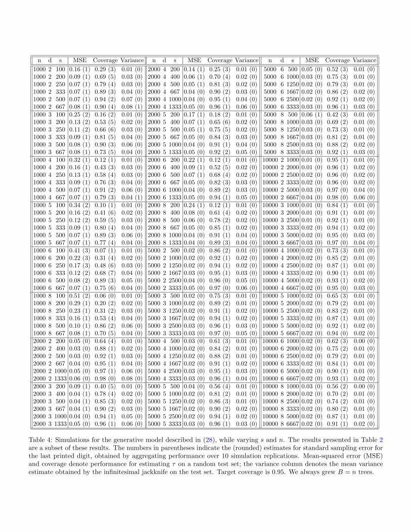
n d s MSE Coverage Variance n d s MSE Coverage Variance n d s MSE Coverage Variance

1000 2 100 0.16 (1) 0.29 (3) 0.01 (0) 2000 4 200 0.14 (1) 0.25 (3) 0.01 (0) 5000 6 500 0.05 (0) 0.52 (3) 0.01 (0)1000 2 200 0.09 (1) 0.69 (5) 0.03 (0) 2000 4 400 0.06 (1) 0.70 (4) 0.02 (0) 5000 6 1000 0.03 (0) 0.75 (3) 0.01 (0)1000 2 250 0.07 (1) 0.79 (4) 0.03 (0) 2000 4 500 0.05 (1) 0.81 (3) 0.02 (0) 5000 6 1250 0.02 (0) 0.79 (3) 0.01 (0)1000 2 333 0.07 (1) 0.89 (3) 0.04 (0) 2000 4 667 0.04 (0) 0.90 (2) 0.03 (0) 5000 6 1667 0.02 (0) 0.86 (2) 0.02 (0)1000 2 500 0.07 (1) 0.94 (2) 0.07 (0) 2000 4 1000 0.04 (0) 0.95 (1) 0.04 (0) 5000 6 2500 0.02 (0) 0.92 (1) 0.02 (0)1000 2 667 0.08 (1) 0.90 (4) 0.08 (1) 2000 4 1333 0.05 (0) 0.96 (1) 0.06 (0) 5000 6 3333 0.03 (0) 0.96 (1) 0.03 (0)1000 3 100 0.25 (2) 0.16 (2) 0.01 (0) 2000 5 200 0.17 (1) 0.18 (2) 0.01 (0) 5000 8 500 0.06 (1) 0.42 (3) 0.01 (0)1000 3 200 0.13 (2) 0.53 (5) 0.02 (0) 2000 5 400 0.07 (1) 0.65 (6) 0.02 (0) 5000 8 1000 0.03 (0) 0.69 (2) 0.01 (0)1000 3 250 0.11 (2) 0.66 (6) 0.03 (0) 2000 5 500 0.05 (1) 0.75 (5) 0.02 (0) 5000 8 1250 0.03 (0) 0.73 (3) 0.01 (0)1000 3 333 0.09 (1) 0.81 (5) 0.04 (0) 2000 5 667 0.05 (0) 0.84 (3) 0.03 (0) 5000 8 1667 0.03 (0) 0.81 (2) 0.01 (0)1000 3 500 0.08 (1) 0.90 (3) 0.06 (0) 2000 5 1000 0.04 (0) 0.91 (1) 0.04 (0) 5000 8 2500 0.03 (0) 0.88 (2) 0.02 (0)1000 3 667 0.08 (1) 0.73 (5) 0.04 (0) 2000 5 1333 0.05 (0) 0.92 (2) 0.05 (0) 5000 8 3333 0.03 (0) 0.92 (1) 0.03 (0)1000 4 100 0.32 (1) 0.12 (1) 0.01 (0) 2000 6 200 0.22 (1) 0.12 (1) 0.01 (0) 10000 2 1000 0.01 (0) 0.95 (1) 0.01 (0)1000 4 200 0.16 (1) 0.43 (3) 0.03 (0) 2000 6 400 0.09 (1) 0.52 (5) 0.02 (0) 10000 2 2000 0.01 (0) 0.96 (1) 0.02 (0)1000 4 250 0.13 (1) 0.58 (4) 0.03 (0) 2000 6 500 0.07 (1) 0.68 (4) 0.02 (0) 10000 2 2500 0.02 (0) 0.96 (0) 0.02 (0)1000 4 333 0.09 (1) 0.76 (3) 0.04 (0) 2000 6 667 0.05 (0) 0.82 (3) 0.03 (0) 10000 2 3333 0.02 (0) 0.96 (0) 0.02 (0)1000 4 500 0.07 (1) 0.91 (2) 0.06 (0) 2000 6 1000 0.04 (0) 0.89 (2) 0.03 (0) 10000 2 5000 0.03 (0) 0.97 (0) 0.04 (0)1000 4 667 0.07 (1) 0.79 (3) 0.04 (1) 2000 6 1333 0.05 (0) 0.94 (1) 0.05 (0) 10000 2 6667 0.04 (0) 0.98 (0) 0.06 (0)1000 5 100 0.34 (2) 0.10 (1) 0.01 (0) 2000 8 200 0.24 (1) 0.12 (1) 0.01 (0) 10000 3 1000 0.01 (0) 0.84 (1) 0.01 (0)1000 5 200 0.16 (2) 0.41 (6) 0.02 (0) 2000 8 400 0.08 (0) 0.61 (4) 0.02 (0) 10000 3 2000 0.01 (0) 0.91 (1) 0.01 (0)1000 5 250 0.12 (2) 0.59 (5) 0.03 (0) 2000 8 500 0.06 (0) 0.78 (2) 0.02 (0) 10000 3 2500 0.01 (0) 0.92 (1) 0.01 (0)1000 5 333 0.09 (1) 0.80 (4) 0.04 (0) 2000 8 667 0.05 (0) 0.85 (1) 0.02 (0) 10000 3 3333 0.02 (0) 0.94 (1) 0.02 (0)1000 5 500 0.07 (1) 0.89 (3) 0.06 (0) 2000 8 1000 0.04 (0) 0.91 (1) 0.04 (0) 10000 3 5000 0.02 (0) 0.95 (0) 0.03 (0)1000 5 667 0.07 (1) 0.77 (4) 0.04 (0) 2000 8 1333 0.04 (0) 0.89 (3) 0.04 (0) 10000 3 6667 0.03 (0) 0.97 (0) 0.04 (0)1000 6 100 0.41 (3) 0.07 (1) 0.01 (0) 5000 2 500 0.02 (0) 0.86 (2) 0.01 (0) 10000 4 1000 0.02 (0) 0.73 (3) 0.01 (0)1000 6 200 0.22 (3) 0.31 (4) 0.02 (0) 5000 2 1000 0.02 (0) 0.92 (1) 0.02 (0) 10000 4 2000 0.02 (0) 0.85 (2) 0.01 (0)1000 6 250 0.17 (3) 0.48 (6) 0.03 (0) 5000 2 1250 0.02 (0) 0.94 (1) 0.02 (0) 10000 4 2500 0.02 (0) 0.87 (1) 0.01 (0)1000 6 333 0.12 (2) 0.68 (7) 0.04 (0) 5000 2 1667 0.03 (0) 0.95 (1) 0.03 (0) 10000 4 3333 0.02 (0) 0.90 (1) 0.01 (0)1000 6 500 0.08 (2) 0.89 (3) 0.05 (0) 5000 2 2500 0.04 (0) 0.96 (0) 0.05 (0) 10000 4 5000 0.02 (0) 0.93 (1) 0.02 (0)1000 6 667 0.07 (1) 0.75 (6) 0.04 (0) 5000 2 3333 0.05 (0) 0.97 (0) 0.06 (0) 10000 4 6667 0.02 (0) 0.95 (0) 0.03 (0)1000 8 100 0.51 (2) 0.06 (0) 0.01 (0) 5000 3 500 0.02 (0) 0.75 (3) 0.01 (0) 10000 5 1000 0.02 (0) 0.65 (3) 0.01 (0)1000 8 200 0.29 (1) 0.20 (2) 0.02 (0) 5000 3 1000 0.02 (0) 0.89 (2) 0.01 (0) 10000 5 2000 0.02 (0) 0.79 (2) 0.01 (0)1000 8 250 0.23 (1) 0.31 (2) 0.03 (0) 5000 3 1250 0.02 (0) 0.91 (1) 0.02 (0) 10000 5 2500 0.02 (0) 0.83 (2) 0.01 (0)1000 8 333 0.16 (1) 0.53 (4) 0.04 (0) 5000 3 1667 0.02 (0) 0.94 (1) 0.02 (0) 10000 5 3333 0.02 (0) 0.87 (1) 0.01 (0)1000 8 500 0.10 (1) 0.86 (2) 0.06 (0) 5000 3 2500 0.03 (0) 0.96 (1) 0.03 (0) 10000 5 5000 0.02 (0) 0.92 (1) 0.02 (0)1000 8 667 0.08 (1) 0.70 (5) 0.04 (0) 5000 3 3333 0.03 (0) 0.97 (0) 0.05 (0) 10000 5 6667 0.02 (0) 0.94 (0) 0.02 (0)2000 2 200 0.05 (0) 0.64 (4) 0.01 (0) 5000 4 500 0.03 (0) 0.61 (3) 0.01 (0) 10000 6 1000 0.02 (0) 0.62 (3) 0.00 (0)2000 2 400 0.03 (0) 0.88 (1) 0.02 (0) 5000 4 1000 0.02 (0) 0.84 (2) 0.01 (0) 10000 6 2000 0.02 (0) 0.75 (2) 0.01 (0)2000 2 500 0.03 (0) 0.92 (1) 0.03 (0) 5000 4 1250 0.02 (0) 0.88 (2) 0.01 (0) 10000 6 2500 0.02 (0) 0.79 (2) 0.01 (0)2000 2 667 0.04 (0) 0.95 (1) 0.04 (0) 5000 4 1667 0.02 (0) 0.91 (1) 0.02 (0) 10000 6 3333 0.02 (0) 0.84 (1) 0.01 (0)2000 2 1000 0.05 (0) 0.97 (1) 0.06 (0) 5000 4 2500 0.03 (0) 0.95 (1) 0.03 (0) 10000 6 5000 0.02 (0) 0.90 (1) 0.01 (0)2000 2 1333 0.06 (0) 0.98 (0) 0.08 (0) 5000 4 3333 0.03 (0) 0.96 (1) 0.04 (0) 10000 6 6667 0.02 (0) 0.93 (1) 0.02 (0)2000 3 200 0.09 (1) 0.40 (5) 0.01 (0) 5000 5 500 0.04 (0) 0.56 (4) 0.01 (0) 10000 8 1000 0.03 (0) 0.56 (2) 0.00 (0)2000 3 400 0.04 (1) 0.78 (4) 0.02 (0) 5000 5 1000 0.02 (0) 0.81 (2) 0.01 (0) 10000 8 2000 0.02 (0) 0.70 (2) 0.01 (0)2000 3 500 0.04 (1) 0.85 (3) 0.02 (0) 5000 5 1250 0.02 (0) 0.86 (3) 0.01 (0) 10000 8 2500 0.02 (0) 0.74 (2) 0.01 (0)2000 3 667 0.04 (1) 0.90 (2) 0.03 (0) 5000 5 1667 0.02 (0) 0.90 (2) 0.02 (0) 10000 8 3333 0.02 (0) 0.80 (2) 0.01 (0)2000 3 1000 0.04 (0) 0.94 (1) 0.05 (0) 5000 5 2500 0.02 (0) 0.94 (1) 0.02 (0) 10000 8 5000 0.02 (0) 0.87 (1) 0.01 (0)2000 3 1333 0.05 (0) 0.96 (1) 0.06 (0) 5000 5 3333 0.03 (0) 0.96 (1) 0.03 (0) 10000 8 6667 0.02 (0) 0.91 (1) 0.02 (0)

Table 4: Simulations for the generative model described in (28), while varying s and n. The results presented in Table 2are a subset of these results. The numbers in parentheses indicate the (rounded) estimates for standard sampling error forthe last printed digit, obtained by aggregating performance over 10 simulation replications. Mean-squared error (MSE)and coverage denote performance for estimating τ on a random test set; the variance column denotes the mean varianceestimate obtained by the infinitesimal jackknife on the test set. Target coverage is 0.95. We always grew B = n trees.

mean-squared error coverageq d CF 10-NN 100-NN CF 10-NN 100-NN2 6 0.04 (0) 0.24 (0) 0.13 (0) 0.92 (1) 0.92 (0) 0.59 (1)4 6 0.06 (0) 0.22 (0) 0.07 (0) 0.87 (1) 0.93 (0) 0.72 (1)6 6 0.08 (0) 0.22 (0) 0.05 (0) 0.75 (1) 0.93 (0) 0.78 (1)2 12 0.04 (0) 0.38 (0) 0.34 (0) 0.86 (1) 0.88 (0) 0.45 (0)4 12 0.08 (0) 0.30 (0) 0.18 (0) 0.76 (1) 0.90 (0) 0.51 (1)6 12 0.12 (0) 0.26 (0) 0.12 (0) 0.59 (1) 0.91 (0) 0.59 (1)

Table 5: Results for a data-generating design where we vary both the number of signalfeatures q and the number of ambient features d. All simulations have n = 5, 000, B = 2, 000and a minimum leaf size of 1, and are aggregated over 20 simulation replicates.

A Additional Simulations

In Table 4, we expand on the simulation results given in Table 2, and present results fordata generated according to (28) all while varying s and n. As expected, we observe abias-variance trade-off: the causal forest is more affected by bias when s is small relativeto n, and by variance when s is larger relative to n. Reassuringly, we observe that ourconfidence intervals obtain close-to-nominal coverage when the mean-squared error matchesthe average variance estimate σ2(X) generated by the infinitesimal jackknife, corroboratingthe hypothesis that failures in coverage mostly arise when the causal forest is bias- insteadof variance-dominated.

Finally, all our experiments relied on settings with strong, low-dimensional structure thatforests could pick up on to improve over k-NN matching. This intuition is formally supportedby, e.g., the theory developed by Biau [2012]. Here, we consider how forests perform whenthe signal is spread out over a larger number of features, and so forests have less upsideover other methods. We find that—as expected—they do not improve much over baselines.Specifically, we generate data with a treatment effect function

τ(x) =4

q

q∑j=1

(1

1 + e−12(xj−0.5)− 1

2

), (30)

where we vary both the number of signal dimensions q and ambient dimensions d. As seenin Table 5, forests vastly improve over k-NN in terms of mean-squared error when q is muchsmaller than d, but that this advantage decreases when d and q are comparable; and actuallydo worse than k-NN when we have a dense signal with d = q = 6. When the signal is dense,all surveyed methods have bad coverage except for 10-NN which, as always, simply has verywide intervals.

B Is Honesty Necessary for Consistency?

Our honesty assumption is the largest divergence between our framework and main-streamapplications of random forests. Following Breiman [2001a], almost all practical implemen-tations of random forests are not honest. Moreover, there has been a stream of recent workproviding theoretical guarantees for adaptive random forests: Scornet et al. [2015] establishrisk consistency under assumptions on the data-generating function, i.e., they show that

30

0.0

0.2

0.4

0.6

n

erro

r

Honest biasHonest RMSEAdapt. biasAdapt. RMSE

100 200 400 800 1600 3200

Figure 3: Comparison of the performance of honest and adaptive causal forests when pre-dicting at x0 = (0, 0, . . . , 0), which is a corner of the support of the features Xi. Both forestshave B = 500 trees, and use a leaf-size of k = 1. We use a subsample size s = n0.8 for adap-tive forests and s = 2n0.8 for honest forests. All results are averaged over 40 replications;we report both bias and root-mean-squared error (RMSE).

the test-set error of forests converges asymptotically to the Bayes risk, Mentch and Hooker[2016] provide results about uncertainty quantification, and Wager and Walther [2015] findthat adaptive trees with growing leaves are in general consistent under fairly weak conditionsand provide bounds on the decay rate of their bias.

However, if we want pointwise centered asymptotic Gaussianity results, then honestyappears to be necessary. Consider the following simple example, where there is no treatmentheterogeneity—and in fact X is independent of W and Y . We are in a randomized controlledtrial, where X ∼ Uniform([0, 1]p) with p = 10 and W ∼ Bernoulli(0.5). The distribution ofY is Yi = 2WiAi+εi, where εi ∼ N

(0, 0.12

)and Ai ∼ Bernoulli(0.05). Thus, the treatment

effect is τ(x) = 0.1 for all x ∈ [0, 1]p. Our goal is to estimate the treatment effect τ(x0) atx0 = (0, 0, . . . , 0).

Results from running both honest and adaptive forests are shown in Figure 3. We seethat honest forests are unbiased regardless of n, and their mean-squared error decreaseswith sample size, as expected. Adaptive forests, in contrast, perform remarkably badly.They have bias that far exceeds the intrinsic sampling variation; and, furthermore, this biasincreases with n. What is happening here is that CART trees aggressively seek to separateoutliers (“Yi ≈ 1”) from the rest of the data (“Yi ≈ 0”) and, in doing so, end up over-representing outliers in the corners of the feature space. As n increases, it appears thatadaptive forests have more opportunities to push outliers into corners of features space andso the bias worsens. This phenomenon is not restricted to causal forests; an earlier technicalreport [Wager, 2014] observed the same phenomenon in the context of plain regression forests.

31

Honest trees do not have this problem, as we do not know where the I-sample outliers will bewhen placing splits using only the J -sample. Thus, it appears that adaptive CART forestsare pointwise biased in corners of x-space.

Finally, we note that this bias phenomenon does not contradict existing consistency re-sults in the literature. Wager and Walther [2015] prove that this bias phenomenon discussedabove can be averted if we use a minimum leaf-size k that grows with n (in contrast, Figure3 uses k = 1). However, their bounds on the bias decays slower than the sampling varianceof random forests, and so their results cannot be used to get centered confidence intervals.

Meanwhile, Scornet et al. [2015] prove that forests are risk-consistent at an average testpoint, and, in fact, the test set error of adaptive forests does decay in the setting of Figure3 as the sample size n grows (although honest forests still maintain a lower test set error).The reason test set error can go to zero despite the bias phenomenon in Figure 3 is that,when n gets large, almost all test points will be far enough from corners that they will notbe affected by the phenomenon from Figure 3.

B.1 Adaptive versus Honest Predictive Error

The discussion above implies that the theorems proved in this paper are not valid for adap-tive forests. That being said, it still remains interesting to ask whether our use of honestforest hurts us in terms of mean-squared error at a random test point, as in the formalismconsidered by, e.g., Scornet et al. [2015]. In this setting, Denil et al. [2014] showed thathonesty can hurt the performance of regression forests on some classic datasets from theUCI repository; however, in a causal inference setting, we might be concerned that the riskof overfitting with adaptive forests is higher since our signals of interest are often quite weak.

We compare the performance of honest and adaptive forests in the setting of Table 2,with d = 8. Here, if we simply run adaptive forests out-of-the-box with the usual minimumleaf size parameter k = 1, they do extremely badly; in fact, they do worse than 50 nearestneighbors. However, if we are willing to increase the minimum leaf size, their performanceimproves.

Figure 4 depicts the root-mean-squared error for both adaptive and honest forests over awide range of choices for the minimum leaf size parameter k. We see that, at their best, bothmethods do comparably. However, honest forests attain good performance over a wide rangeof choices for k, including our default choice k = 1, whereas adaptive forests are extremelysensitive to choosing a good value of k. We also note that the optimum k = 64 for adaptiveforests is quite far from standard choices advocated in practice; such as k = 5 recommendedby Breiman [2001a] for regression forests, k = 7 in the cforest function used by Stroblet al. [2007], or k = 10 recommended by Meinshausen [2006] for quantile regression. Thus,it appears that accurately tuning adaptive forests in this setting may present a challengeand, overall, a practitioner may prefer honest forests even based on their mean-squared errorcharacteristics alone.

C Proofs

Notation. Throughout the appendix we use the following notation to describe asymp-totic scalings: f(s) ∼ g(s) means that lims→∞ f(s)/g(s) = 1, f(s) & g(s) means thatlim infs→∞ f(s)/g(s) ≥ 1 and f(s) . g(s) is analogous, f(s) = O(g(s)) means that f(s) .C g(s) for some C > 0, f(s) = Ω(g(s)) means that f(s) & c g(s) for some c > 0, and finallyf(s) = o(g(s)) means that lim sups→∞ f(s)/g(s) = 0.

32

0.2

0.3

0.4

0.5

Minimum Leaf Size

Roo

t−M

ean−

Squ

ared

Err

or

1 2 4 8 16 32 64 128 256

Honest ForestAdaptive Forest

Figure 4: Comparison of the root-mean-squared error of honest and adaptive forests in thesetting of Table 2, with d = 8. Honest forests use s = 2500 (i.e., |I| = 1250) while adaptiveforests use s = 1250, such that both methods grow trees of the same depth. Both forestshave B = 500, and results are averaged over 100 simulation replications.

Proof of Theorem 1. Given the statements of Theorem 8 and Theorem 9, it only remains toshow that (15) holds with E [µn(x)] replaced with µ(x). To do so, it suffices to show that|E [µn (x)]− µ(x)| /σn (x) → 0; the rest follows from Slutsky’s lemma. Now, recall that byTheorem 3,

|E [µn (x)]− µ(x)| = O

(n− β2

log((1−α)−1)π−1d log(α−1)

).

Meanwhile, from Theorem 5 and the proof of Theorem 8, we see that

σ2n(x) & Cf, d

s

n

Var [T ]

log(s)d.

By honesty of T , Var [T ] & Var[Y∣∣X = x

]/ |i : Xi ∈ L(x)| ≥ Var

[Y∣∣X = x

]/(2k), and

so

σ2n(x) &

Cf, d2k

s

n

Var[Y∣∣X = x

]log(s)d

= Ω(nβ−1−ε)

for any ε > 0. It follows that

|E [µn (x)]− µ(x)|σn (x)

= O

n 12

(1+ε−β

(1+

log((1−α)−1)π−1d log(α−1)

)) .

33

The right-hand-side bound converges to 0 for some small enough ε > 0 provided that

β >

1 +log(

(1− α)−1)

π−1d log (α−1)

−1

= 1−

1 +d

π

log(α−1

)log(

(1− α)−1)−1

= βmin.

C.1 Bounding the Bias of Regression Trees

Proof of Lemma 2. Let c(x) be the number of splits leading to the leaf L(x), and let cj(x) bethe number of these splits along the j-th coordinate. By regularity, we know that sαc(x) ≤2k − 1, and so c(x) ≥ log(s/(2k − 1))/ log(α−1). Thus, because the tree is a random splittree, cj(x) we have the following stochastic lower bound for cj(x):

cj(x)d≥ Binom

(log (s/(2k − 1))

log (α−1);π

d

). (31)

By Chernoff’s inequality, it follows that

P[cj (x) ≤ π

d

log (s/(2k − 1))

log (α−1)(1− η)

]≤ exp

[−η

2

2

log (s/(2k − 1))

π−1d log (α−1)

](32)

=

(s

2k − 1

)− η22 1

π−1d log(α−1).

Meanwhile, again by regularity, we might expect that diamj (L (x)) should less than (1− α)cj(x)

,at least for large n. This condition would hold directly if the regularity condition from Defini-tion 4 were framed in terms of Lebesgue measure instead of the number of training examplesin the leaf; our task is to show that it still holds approximately in our current setup.

Using the methods developed in Wager and Walther [2015], and in particular theirLemma 12, we can verify that, with high probability and simultaneously for all but thelast O (log log n) parent nodes above L(x), the number of training examples inside the nodedivided by n is within a factor 1 + o(1) of the Lebesgue measure of the node. From this, weconclude that, for large enough s, with probability greater than 1− 1/s

diamj (L (x)) ≤ (1− α+ o(1))(1+o(1))cj(x)

,

or, more prosaically, that

diamj (L (x)) ≤ (1− α)0.991 cj(x)

.

Combining this results with the above Chernoff bound yields the desired inequality. Here,replacing 0.991 with 0.99 in the bound lets us ignore the 1/s asymptotic failure probabilityof the concentration result used above.

Finally, we note that with double-sample trees, all the “s” terms in the above argumentneed to be replaced by “s/2”; this additional factor 2, however, does not affect the finalresult.

34

Proof of Theorem 3. We begin with two observations. First, by honesty,

E [T (x; Z)]− E[Y∣∣X = x

]= E

[E[Y∣∣X ∈ L (x)

]− E

[Y∣∣X = x

]].

Second, by Lipschitz continuity of the conditional mean function,∣∣E [Y ∣∣X ∈ L (x)]− E

[Y∣∣X = x

]∣∣ ≤ C diam (L (x)) ,

where C is the Lipschitz constant. Thus, in order to bound the bias under both Lipschitzand honesty assumptions, it suffices to bound the average diameter of the leaf L(x).

To do so, we start by plugging in η =√

log((1− α)−1 in the bound from Lemma 2.Thanks our assumption that α ≤ 0.2, we see that η ≤ 0.48 and so 0.99 · (1− η) ≥ 0.51; thus,a union bound gives us that, for large enough s,

P

diam (L(x)) ≥√d

(s

2k − 1

)−0.51log((1−α)−1)

log(α−1)πd

≤ d ( s

2k − 1

)− 12

log((1−α)−1)log(α−1)

πd

.

The Lipschitz assumption lets us bound the bias on the event that that diam(L(x)) satisfiesthis bound. Thus, for large s, we find that

∣∣E [T (x; Z)]− E[Y∣∣X = x

]∣∣ . d

(s

2k − 1

)− 12

log((1−α)−1)log(α−1)

πd

×

(sup

x∈[0, 1]d

E[Y∣∣X = x

]− infx∈[0, 1]d

E[Y∣∣X = x

]),

where supx E[Y∣∣X = x

]−infx E

[Y∣∣X = x

]= O (1) because the conditional mean function

is Lipschitz continuous. Finally, since a forest is just an average of trees, the above resultalso holds for µ(x).

C.2 Bounding the Incrementality of Regression Trees

Proof of Lemma 4. First, we focus on the case where f is constant, i.e., the features Xi havea uniform distribution over [0, 1]d. To begin, recall that the Si denote selection weights

T (x; Z) =

s∑i=1

SiYi where Si =

|i : Xi ∈ L(x; Z)|−1

if Xi ∈ L(x; Z),

0 else,

where L(x; Z) denotes the leaf containing x. We also define the quantities

Pi = 1 (Xi is a k-PNN of x) .

Because T is a k-PNN predictor, Pi = 0 implies that Si = 0, and, moreover, |i : Xi ∈ L(x; Z)| ≥k; thus, we can verify that

E[S1

∣∣Z1

]≤ 1

kE[P1

∣∣Z1

].

The bulk of the proof involves showing that

P[E[P1

∣∣Z1

]≥ 1

s2

]. k

2d+1 log (s)d

(d− 1)!

1

s; (33)

35

by the above argument, this immediately implies that

P[E[S1

∣∣Z1

]≥ 1

k s2

]. k

2d+1 log (s)d

(d− 1)!

1

s. (34)

Now, by exchangeability of the indices i, we know that

E[E[S1

∣∣Z1

]]= E [S1] =

1

sE

[s∑i=1

Si

]=

1

s,

moreover, we can verify that

P[E[S1

∣∣Z1

]≥ 1

ks2

]E[E[S1

∣∣Z1

] ∣∣E [S1

∣∣Z1

]≥ 1

ks2

]∼ 1

s.

By Jensen’s inequality, we then see that

E[E[S1

∣∣Z1

]2] ≥ P[E[S1

∣∣Z1

]≥ 1

ks2

]E[E[S1

∣∣Z1

] ∣∣E [S1

∣∣Z1

]≥ 1

ks2

]2

∼ s−2

P[E[S1

∣∣Z1

]≥ 1

ks2

]which, paired with (34), implies that

E[E[S1

∣∣Z1

]2]&

(d− 1)!

2d+1 log (s)d

1

k s.

This is equivalent to (20) because E[E[S1

∣∣Z1

]]2= 1/s2 is negligibly small.

We now return to establishing (33). Recall that X1, ..., Xs are independently and uni-formly distributed over [0, 1]d, and that we are trying to find points that are k-PNNs of aprediction point x. For now, suppose that x = 0. We know that X1 is a k-PNN of 0 if andonly if there are at most 2k − 2 other points Xi such that Xij ≤ X1j for all j = 1, ..., d(because the X have a continuous density, there will almost surely be no ties). Thus,

Ex=0

[P1

∣∣Z1

]= P

Binomial

s− 1;

d∏j=1

X1j

≤ 2k − 2

(35)

≤(s− 1

2k − 2

)1−d∏j=1

X1j

s−2k+1

≤ s2k−2

1−d∏j=1

X1j

s−2k+1

,

where the second inequality can be understood as a union bound over all sets of s− 2k + 1

Bernoulli realizations that could be simultaneously 0. We can check that X1jd= e−Ej where

Ej is a standard exponential random variable, and so

Ex=0

[P1

∣∣Z1

] d≤ s2k−2

1− exp

− d∑j=1

Ej

s−2k+1

,

36

where Ad≤ B means that B −A ≥ 0 almost surely. Thus,

Px=0

[E[P1

∣∣Z1

]≥ 1

s2

]

≤ P

s(2k−2)

1− exp

− d∑j=1

Ej

s−2k+1

≥ 1

s2

= P

exp

− d∑j=1

Ej

≤ 1−(

1

s2k

) 1s−2k+1

= P

d∑j=1

Ej ≥ − log

(1− exp

[−2k

log (s)

s− 2k + 1

]) .Notice that this quantity goes to zero as s gets large. The sum of d standard exponentialrandom variables has a gamma distribution with shape d and scale 1, and

P

d∑j=1

Ej ≥ c

=Γ (d, c)

(d− 1)!,

where Γ is the upper incomplete gamma function. It is well known that

limc→∞

Γ (d, c)

cd−1 e−c= 1,

and so

Px=0

[E[P1

∣∣Z1

]≥ 1

s2

]

.

(− log

(1− exp

[−2k log(s)

s−2k+1

]))d−1 (1− exp

[−2k log(s)

s−2k+1

])(d− 1)!

.

We can check that

1− exp

[−2k

log (s)

s− 2k + 1

]∼ 2k

log (s)

s,

letting us simplify the above expression to

Px=0

[E[P1

∣∣Z1

]≥ 1

s2

].

2k

(d− 1)!

log (s)d

s. (36)

We thus have obtained a tight expression for our quantity of interested for a prediction pointat x = 0.

In the case x 6= 0, the ambient space around x can be divided into 2d quadrants. Inorder to check whether Xi is a PNN, we only need to consider other points in the samequadrant, as no point in a different quadrant can prevent Xi from being a PNN. Now, indexthe quadrants by l = 1, ..., 2d, and let vl be the volume of the l-th quadrant. By applying

37

(36) on the l-th quadrant alone, we see that the probability of E[P1

∣∣Z1

]≥ 1

s2 given thatX1 is in the l-the quadrant is asymptotically bounded on the order of

2k

(d− 1)!

log (s)d

vl s.

Summing over all quadrants, we find that

Px=0

[E[P1

∣∣Z1

]≥ 1

s2

].

∑l:vl>0

vl2k

(d− 1)!

log (s)d

vl s

= |l : vl > 0| 2k

(d− 1)!

log (s)d

s

≤ k 2d+1

(d− 1)!

log (s)d

s,

thus establishing (33). Finally, to generalize to bounded densities f , we note that if f(x) ≤ Cfor all x ∈ [0, 1]d, then

Ex=0

[P1

∣∣Z1

]≤ P

Binomial

s− 1; C

d∏j=1

X1j

≤ 2k − 2

,and the previous argument goes though.

Proof of Theorem 5. Our main task is to show that if T is a regular tree and Var[Y∣∣X = x

]>

0, thenVar

[E[T (x; Z)

∣∣Z1

]]& Var

[E[S1

∣∣Z1

]]Var

[Y∣∣X = x

]. (37)

Given this result, Lemma 4 then implies that

Var[E[T (x; Z)

∣∣Z1

]]&

1

k

ν (s)

sVar

[Y∣∣X = x

].

Moreover, by Theorem 3, we know that

E[Yi∣∣Xi ∈ L (x; Z)

]→p E

[Y∣∣X = x

], and

E[Y 2i

∣∣Xi ∈ L (x; Z)]→p E

[Y 2∣∣X = x

],

and so

kVar [T (x; Z)] ≤ |i : Xi ∈ L (x; Z)| ·Var [T (x; Z)]→p Var[Y∣∣X = x

],

because k remains fixed while the leaf size gets smaller. Thus, we conclude that

Var[T (x; Z)

]Var [T (x; Z)]

& ks Var

[E[T (x; Z)

∣∣Z1

]]Var

[Y∣∣X = x

] & ν (s) ,

as claimed.

38

Now, in order to verify (37), we first recall that by Lemma 4

Var[E[S1

∣∣Z1

]]= Ω

(1

s log (s)d

). (38)

Thus, any terms that decay faster than the right-hand-side rate can safely be ignored inestablishing (37). We begin by verifying that we can take the leaf L(x) containing x to havea small diameter diam(L(x)). Define the truncated tree predictor

T ′ (x; Z) = T (x; Z) 1(

diam (L(x)) ≤ s−ω), where ω =

1

2

π

d

log(

(1− α)−1)

log (α−1),

and define similarly the truncated selection variables S′i = Si 1(diam (L(x)) ≤ s−ω). Now,thanks to the ANOVA decomposition (3rd line), we see that

Var[E[T ′ (x; Z)

∣∣Z1

]− E

[T (x; Z)

∣∣Z1

]]= Var

[E[T (x; Z) 1

(diam (L(x)) > s−ω

) ∣∣Z1

]]≤ 1

sVar

[T (x; Z) 1

(diam (L(x)) > s−ω

)]≤

supx∈[0, 1]dE[Y 2∣∣X = x

]s

P[diam (L(x)) > s−ω

],

where the sup term is bounded by Lipschitz-continuity of the second moment of Y . Thus,by Lemma 2, the variance of the difference between E

[T ′∣∣Z1

]and E

[T∣∣Z1

]decays faster

than the target rate (38), and so

Var[E[T (x; Z)

∣∣Z1

]]∼ Var

[E[T ′ (x; Z)

∣∣Z1

]],

provided that T ′ satisfies (37), as we will see it does. By the same argument, we also notethat

Var[E[S′1∣∣Z1

]]∼ Var

[E[S1

∣∣Z1

]].

We can now proceed to analyze T ′ instead of T .Recall that our goal is to provide a lower bound on the variance of the expectation of

T ′(x; Z) conditionally on Z1. First, an elementary decomposition shows that

Var[E[T ′(x; Z)

∣∣Z1

]]= Var

[E[T ′(x; Z)

∣∣X1

]]+ Var

[E[T ′(x; Z)

∣∣X1, Y1

]− E

[T ′(x; Z)

∣∣X1

]]≥ Var

[E[T ′(x; Z)

∣∣X1, Y1

]− E

[T ′(x; Z)

∣∣X1

]],

and so it suffices to provide a lower bound for the latter term. Next we note that, thanksto honesty as in Definition 2, part (a), and i.i.d. sampling,

E[T ′(x; Z)

∣∣X1, Y1

]− E

[T ′(x; Z)

∣∣X1

]= E

[S′1∣∣X1

] (Y1 − E

[Y1

∣∣X1

]).

Because of honesty and our Lipschitz assumption, the above implies that

Var[E[T ′(x; Z)

∣∣X1, Y1

]− E

[T ′(x; Z)

∣∣X1

]]= Var

[E[S′1∣∣X1

](Y1 − µ(x))

]+O

(E[S′21]s−2ω

),

39

where we note that the error term decays as s−(1+2ω), which will be prove to be negligiblerelative to the main term. Finally, we can verify that

Var[E[S′1∣∣X1

](Y1 − µ(x))

](39)

= E[E[S′1∣∣X1

]2 E[(Y1 − µ (x))

2 ∣∣X1

]]− E

[E[S′1∣∣X1

]E[Y1 − µ(x)

∣∣X1

]]2.

Now, because the first two conditional moments of Y given X are Lipschitz, and sinceE[S′1∣∣X1

]is 0 for ‖X1 − x‖2 > s−ω thanks to our truncating argument, we see that

E[E[S′1∣∣X1

]2 E[(Y1 − µ (x))

2 ∣∣X1

]]∼ E

[E[S′1∣∣X1

]2]Var

[Y∣∣X = x

]∼ E

[E[S1

∣∣X1

]2]Var

[Y∣∣X = x

].

Meanwhile, the second term in the expansion (39) is of order 1/s2 and thus negligible. Torecap, we have shown that a version of (37) holds with T replaced by T ′; and so (37) mustalso hold thanks to the previously established coupling result.

Proof of Corollary 6. For a double sample tree, we start by noting that

Var[T]

= sVar[E[T∣∣Z1

]]= sVar

[E[1 (1 ∈ I)T

∣∣Z1

]+ E

[1 (1 6∈ I)T

∣∣Z1

]]≥ s

2Var

[E[1 (1 ∈ I)T

∣∣Z1

]]− sVar

[E[1 (1 6∈ I)T

∣∣Z1

]]∼ s

8Var

[E[T∣∣Z1

] ∣∣ 1 ∈ I]− s

4Var

[E[T∣∣Z1

] ∣∣ 1 6∈ I] ,where to verify the last line we note that P

[1 ∈ I

∣∣Z1

]= bs/2c regardless of Z1. Now, an

immediate application of Theorem 5 shows us that

bs/2cVar[E[T∣∣Z1

] ∣∣ 1 ∈ I] & Cf, d/

log (s)d

Var [T ] ,

which corresponds to the rate we seek to establish. Meanwhile, by standard results goingback to Hoeffding [1948],

ds/2eVar[E[T∣∣Z1

] ∣∣ 1 6∈ I] ≤ Var[E[T∣∣ Zj : j 6∈ I

] ∣∣ I] ;

then, Lemma 2 and the argument used to establish Theorem 3 imply that

Var[E[T∣∣ Zj : j 6∈ I

] ∣∣ I] = O

(s−

log((1−α)−1)log(α−1)

πd

),

and so the term arising under the 1 6∈ I condition is negligibly small.

C.3 Properties of Subsampled Incremental Base Learners

The results presented in this section rely heavily on the Efron-Stein ANOVA decomposition,summarized here for convenience. Suppose we have any symmetric function T : Ωn → R,and suppose that Z1, ..., Zn are independent and identically distributed on Ω such thatVar [T (Z1, ..., Zn)] < ∞. Then Efron and Stein [1981] show that there exist functionsT1, ..., Tn such that

T (Z1, ..., Zn) = E [T ] +

n∑i=1

T1 (Zi) +∑i<j

T2 (Zi, Zj) + ...+ Tn (Z1, ..., Zn) , (40)

40

and that all 2n − 1 random variables on the right side of the above expression are all mean-zero and uncorrelated. It immediately follows that

Var [T ] =

n∑k=1

(n

k

)Vk, where Vk = Var [Tk (Z1, ..., Zk)] . (41)

For our purposes, it is also useful to note that the Hajek projection T can be written as

T (Z1, ..., Zn) = E [T ] +

n∑i=1

T1 (Zi) , and Var[T]

= nV1.

Thus, the ANOVA decomposition provides a convenient abstract framework for analyzingour quantities of interest.

Proof of Lemma 7. Applying the ANOVA decomposition to the individual trees T , we seethat a random forest estimator µ(x) of the form (12) can equivalently be written as

µ (x; Z1, ..., Zn) = E [T ] +

(n

s

)−1((

n− 1

s− 1

) n∑i=1

T1 (Zi)

+

(n− 2

s− 2

)∑i<j

T2 (Zi, Zj) + ...+∑

i1<...<is

Ts (Zi1 , ..., Zis)

).

The above formula holds because each training point Zi appears in(n−1s−1

)out of

(ns

)possible

subsamples of size s, each pair (Zi, Zj) appears is(n−2s−2

)subsets, etc.

Now, we can also show that the Hajek projection of µ is

˚µ (x; Z1, ..., Zn) = E [T ] +s

n

n∑i=1

T1 (Zi) .

As with all projections [Van der Vaart, 2000],

E[(µ(x)− ˚µ(x)

)2]

= Var[µ(x)− ˚µ(x)

].

Recall that the Tk (·) are all pairwise uncorrelated. Thus, using the notation sk = s ·(s− 1) · · · (s− k) it follows that

E[(µ(x)− ˚µ(x)

)2]

=

s∑k=2

(sknk

)2(n

k

)Vk,

=

s∑k=2

sknk

(s

k

)Vk,

≤ s2

n2

s∑k=2

(s

k

)Vk,

≤ s2

n2Var [T ] ,

where on the last line we used (41). We recover the stated result by noticing that s2/n2 ≤s2/n2 for all 2 ≤ s ≤ n.

41

Proof of Theorem 8. Using notation from the previous lemma, let σ2n = s2/nV1 be the

variance of ˚µ. We know that

σ2n =

s

nsV1 ≤

s

nVar [T ] ,

and so σn → 0 as desired. Now, by Theorem 5 or Corollary 6 combined with Lemma 7, wefind that

1

σ2n

E[(µ (x)− ˚µ (x)

)2]≤( sn

)2 Var [T ]

σ2n

=s

nVar [T ]

/Var

[T]

.s

n

log (s)d

Cf, d/4

→ 0

by hypothesis. Thus, by Slutsky’s lemma, it suffices to show that (22) holds for the Hajek

projection of the random forest ˚µ(x).

By our definition of σn, all we need to do is check that ˚µ is asymptotically normal. Oneway to do so is using the Lyapunov central limit theorem [e.g., Billingsley, 2008]. Writing

˚µ(x) =s

n

n∑i=1

(E[T∣∣Zi]− E [T ]

),

it suffices to check that

limn→∞

n∑i=1

E[∣∣E [T ∣∣Zi]− E [T ]

∣∣2+δ] / ( n∑

i=1

Var[E[T∣∣Zi]])1+δ/2

= 0. (42)

Using notation from Section 3.3.1, we write T =∑ni=1 SiYi. Thanks to honesty, we can

verify that for any index i > 1, Yi is independent of Si conditionally on Xi and Z1, and so

E[T∣∣Z1

]− E [T ] = E

[S1

(Y1 − E

[Y1

∣∣X1

]) ∣∣Z1

]+

(E

[n∑i=1

SiE[Yi∣∣Xi

] ∣∣Z1

]− E [T ]

).

Note that the two right-hand-side terms above are both mean-zero. By Jensen’s inequality,we also have that

2−(1+δ) E[∣∣E [T ∣∣Z1

]− E [T ]

∣∣2+δ]≤ E

[∣∣E [S1

(Y1 − E

[Y1

∣∣X1

]) ∣∣Z1

]∣∣2+δ]

+ E

∣∣∣∣∣E[

n∑i=1

SiE[Yi∣∣Xi

] ∣∣Z1

]− E [T ]

∣∣∣∣∣2+δ .

Now, again by honesty, E[S1

∣∣Z1

]= E

[S1

∣∣X1

], and so our uniform (2+δ)-moment bounds

on the distribution of Yi conditional on Xi implies that

E[∣∣E [S1

(Y1 − E

[Y1

∣∣X1

]) ∣∣Z1

]∣∣2+δ]

= E[E[S1

∣∣X1

]2+δ ∣∣Y1 − E[Y1

∣∣X1

]∣∣2+δ]

≤ME[E[S1

∣∣X1

]2+δ]≤ME

[E[S1

∣∣X1

]2],

42

because S1 ≤ 1. Meanwhile, because E[Y∣∣X = x

]is Lipschitz, we can define u :=

sup∣∣E [Y ∣∣X = x

]∣∣ : x ∈ [0, 1]d

, and see that

E

∣∣∣∣∣E[

n∑i=1

SiE[Yi∣∣Xi

] ∣∣Z1

]− E [T ]

∣∣∣∣∣2+δ ≤ (2u)δ Var

[E

[n∑i=1

SiE[Yi∣∣Xi

] ∣∣Z1

]]

≤ 21+δu2+δ(E[E[S1

∣∣Z1

]2]+ Var

[(n− 1)E

[S2

∣∣Z1

]])≤ (2u)2+δE

[E[S1

∣∣X1

]2].

Thus, the condition we need to check simplifies to

limn→∞

nE[E[S1

∣∣X1

]2] / (nVar

[E[T∣∣Z1

]])1+δ/2= 0.

Finally, as argued in the proofs of Theorem 5 and Corollary 6,

Var[E[T∣∣Z1

]]= Ω

(E[E[S1

∣∣X1

]2]Var

[Y∣∣X = x

]).

Because Var[Y∣∣X = x

]> 0 by assumption, we can use Lemma 4 to conclude our argument,

noting that (nE

[E[S1

∣∣X1

]2])−δ/2.

(Cf, d2k

n

s log(s)d

)−δ/2,

which goes to 0 thanks to our assumptions on the scaling of s (and the factor 2 comes frompotentially using a double-sample tree).

Proof of Theorem 9. Let F denote the distribution from which we drew Z1, ..., Zn. Then,the variance σ2

n of the Hajek projection of µ(x) is

σ2n =

n∑i=1

(EZ∼F

[µ(x)

∣∣Zi]− EZ∼F [µ(x)])2

=s2

n2

n∑i=1

(EZ∼F

[T∣∣Zi]− EZ∼F [T ]

)2,

whereas we can check that the infinitesimal jackknife as defined in (8) is equal to

VIJ =n− 1

n

(n

n− s

)2s2

n2

n∑i=1

(EZ∗⊂F

[T∣∣Z∗1 = Zi

]− EZ∗⊂F [T ]

)2,

where F is the empirical distribution on Z1, ..., Zn. Recall that we are sampling the Z∗

from F without replacement.It is useful to write our expression of interest VIJ using the Hajek projection T of T :

VIJ =n− 1

n

(n

n− s

)2s2

n2

n∑i=1

(Ai +Ri)2, where

Ai = EZ∗⊂F

[T∣∣Z∗1 = Zi

]− EZ∗⊂F

[T]

and

Ri = EZ∗⊂F

[T − T

∣∣Z∗1 = Zi

]− EZ∗⊂F

[T − T

].

43

As we show in Lemma 12, the main effects Ai give us σ2n, in that

1

σ2n

s2

n2

n∑i=1

A2i →p 1. (43)

Meanwhile, Lemma 13 establishes that the Bi all satisfy

E[R2i

].

2

nVar [T (x; , Z1, ..., Zs)] , (44)

and so

E

[s2

n2

n∑i=1

R2i

].

2 s2

n2Var [T (x; , Z1, ..., Zs)]

.2 s

nlog (n)

dσ2n.

Because all terms are positive and s log (n)d/n goes to zero by hypothesis, Markov’s inequal-

ity implies that

1

σ2n

s2

n2

n∑i=1

R2i →p 0.

Using Cauchy-Schwarz to bound the cross terms of the formAiRi, and noting that limn→∞ n(n−1)/(n− s)2 = 1, we can thus conclude that VIJ/σ

2n converges in probability to 1.

Lemma 12. Under the conditions of Theorem 9, (43) holds.

Proof. We can write

Ai = EZ∗⊂F

[T∣∣Z∗1 = Zi

]− EZ∗⊂F

[T]

=(

1− s

n

)T1 (Zi) +

(s− 1

n− 1− s

n

)∑j 6=i

T1 (Zj) ,

and so our sum of interest is asymptotically unbiased for σ2n:

E

[n− 1

n

(n

n− s

)2s2

n2

n∑i=1

A2i

]=s2

nE[T1 (Z)

2]

=s

nVar

[T (Z1, ..., Zs)

]= σ2

n.

Finally, to establish concentration, we first note that the above calculation also implies that

σ−2n

s2

n2

∑ni=1 (Ai − T1(Zi))

2 →p 0. Meanwhile, following the argumentation in the proof ofTheorem 8, we can apply (2 + δ)-moment bounds on Yi − E

[Yi∣∣Xi

]to verify that

limu→∞

limn→∞

(E[T 2

1 (Z1)]− E

[min

u, T 2

1 (Z1)])

= 0,

and so we obtain can apply a truncation-based argument to derive a weak law of large

numbers for triangular arrays for σ−2n

s2

n2

∑ni=1 T

21 (Zi).

44

Lemma 13. Under the conditions of Theorem 9, (44) holds.

Proof. Without loss of generality, we establish (44) for R1. Using the ANOVA decomposition(40), we can write our term of interest as

R1 = EZ∗⊂F

[T − T

∣∣Z∗1 = Z1

]− EZ∗⊂F

[T − T

]=

(s− 1

n− 1−(s

2

)/(n2

)) n∑i=2

T2 (Z1, Zi)

+

((s− 1

2

)/(n− 1

2

)−(s

2

)/(n2

)) ∑2≤i<j≤n

T2 (Zi, Zj)

+

((s− 1

2

)/(n− 1

2

)−(s

3

)/(n3

)) ∑2≤i<j≤n

T3 (Z1, Zi, Zj)

+

((s− 1

3

)/(n− 1

3

)−(s

3

)/(n3

)) ∑2≤i<j<k≤n

T3 (Zi, Zj , Zk)

+ . . .

Because all the terms in the ANOVA expansion are mean-zero and uncorrelated, we seeusing notation from (41) that

E[R2

1

]= (n− 1)

(s− 1

n− 1−(s

2

)/(n2

))2

V2

+

(n− 1

2

)((s− 1

2

)/(n− 1

2

)−(s

2

)/(n2

))2

V2

+

(n− 1

2

)((s− 1

2

)/(n− 1

2

)−(s

3

)/(n3

))2

V3

+

(n− 1

3

)((s− 1

3

)/(n− 1

3

)−(s

3

)/(n3

))2

V3

+ . . .

Recall thats∑

k=1

(s

k

)Vk = Var [T (Z1, ..., Zs)] .

The above sum is maximized when all the variance is contained in second-order terms, and(s2

)V2 = Var [T ]. This implies that

E[R2

1

]. (n− 1)

(s− 1

n− 1−(s

2

)/(n2

))2(s

2

)−1

Var [T (Z1, ..., Zs)]

∼ 2

nVar [T (Z1, ..., Zs)] ,

thus completing the proof.

45

Proof of Proposition 10. Let N∗i denote whether or not the i-training example was used fora subsample, as in (13). For trivial trees

T (x; ξ, Zi1 , ..., Zis) =1

s

s∑j=1

Yij

we can verify that for any i = 1, ..., n, E∗ [µ∗]E [N∗i ] = s/n Y ,

E∗ [µ∗N∗1 ] =s

n

(Yis

+s− 1

s

nY − Yin− 1

)=

1

n

n− sn− 1

Yi +s− 1

n− 1Y , and

Cov∗ [µ∗, N∗i ] =1

n

n− sn− 1

Yi +

(s− 1

n− 1− s

n

)Y =

1

n− 1

n− sn

(Yi − Y

).

Thus, we find that

VIJ =n− 1

n

(n

n− s

)2 n∑i=1

Cov∗ [µ∗, N∗i ]2

=1

n (n− 1)

n∑i=1

(Yi − Y

)2= Vsimple,

as we sought to verify.

C.4 Extension to Causal Forests

Proof of Theorem 11. Our argument mirrors the proof of Theorem 1. The main steps involvebounding the bias of causal forests with an analogue to Theorem 3 and their incrementalityusing an analogue to Theorem 5. In general, we find that the same arguments as usedwith regression forests go through, but the constants in the results get worse by a factorε depending on the amount of overlap (6). Given these results, the subsampling-basedargument from Section 3.3.2 can be reproduced almost verbatim, and the final proof ofTheorem 11 is identical to that of Theorem 1 presented at the beginning of Appendix C.

Bias. Under the conditions of Lemma 2, suppose that E[Y (0)

∣∣X = x]

andE[Y (1)

∣∣X = x]

are Lipschitz continuous, that the trees Γ comprising the random forestare honest, and, moreover, that the overlap condition (6) holds for some ε > 0. These con-ditions also imply that |E[Y (0)

∣∣X = x]|, |E[Y (1)∣∣X = x]| ≤M for some constant M , for all

x ∈ [0, 1]d. Then, provided that α ≤ 0.2, the bias of the random forest at x is bounded by

|E [τ (x)]− τ (x)| . 2M d

(ε s

2k − 1

)− 12

log((1−α)−1)log(α−1)

πd

.

To establish this claim, we first seek with an analogue to Lemma 2, except now s in (31) isreplaced by smin, i.e., the minimum of the number of cases (i.e., observations with Wi = 1)or controls (i.e., observations with Wi = 0) in the sample. A straight-forward computationthen shows that smin/s & ε, and that a variant of (32) where we replace s with εs still holdsfor large s. Next, to bound the bias itself, we start by applying unconfoundedness as in (25);

46

then, the argument of Theorem 3 goes through without modifications, provided we replaceevery instance of “s” with “εs”.

Incrementality. Suppose that the conditions of Lemma 4 hold and that Γ is an hon-est k-regular causal tree in the sense of Definitions 2b and 4b. Suppose moreover thatE[Y (0/1)

∣∣X = x]

and Var[Y (0/1)

∣∣X = x]

are all Lipschitz continuous at x, and thatVar

[Y∣∣X = x

]> 0. Suppose, finally, that the overlap condition (6) holds with ε > 0.

Then T is ν (s)-incremental at x with

ν (s) = εCf, d/

log (s)d,

where Cf, d is the constant from Lemma 4.To prove this claim, we again focus on the case where f(x) = 1, in which case we use

Cf, d = 2−(d+1) (d− 1)!. We begin by setting up notation as in the proof of Lemma 4. Wewrite our causal tree as Γ (x; Z) =

∑si=1 SiYi, where

Si =

|i : Xi ∈ L(x; Z) , Wi = 1|−1

if Xi ∈ L(x; Z) and Wi = 1,

− |i : Xi ∈ L(x; Z) , Wi = 0|−1if Xi ∈ L(x; Z) and Wi = 0,

0 else,

where L(x; Z) denotes the leaf containing x, and let

PWi = 1 (Xi is a k-PNN of x among points with treatment status Wi) .

Finally, in a break from Lemma 4, define wmin(x; Z) as the minority class within the leafL(x; Z); more formally,

wmin = 1 (|i : Xi ∈ L(x; Z) , Wi = 1| ≤ |i : Xi ∈ L(x; Z) , Wi = 0|) .

By regularity of Γ, we know that the leaf L(x; Z) can contain at most 2k− 1 examples fromits minority class, and so PWi = 0 and W = wmin together imply that Si = 0. Thus, we canverify that

E[|S1| 1 (W1 = wmin)

∣∣Z1

]≤ 1

kE[PW1

∣∣Z1

].

We are now ready to use the same machinery as before. The random variables PW1 nowsatisfy

P

[E[PW1

∣∣Z1

]≥ 1

s2 P [W = W1]2

]. k

2d+1 log (s)d

(d− 1)!

1

sP [W = W1];

by the above argument and ε-overlap (6), this immediately implies that

P[E[|S1| 1

(W1 = wmin

∣∣Z1

)]≥ 1

k ε2 s2

]. k

2d+1 log (s)d

(d− 1)!

1

εs.

By construction, we know that

E[E[|S1| 1 (W1 = wmin)

∣∣Z1

]]= E [|S1| 1 (W1 = wmin)] =

1

s,

which by the same argument as before implies that

E[E[|S1| 1 (W1 = wmin)

∣∣Z1

]2]&

(d− 1)!

2d+1 log (s)d

ε

k s.

47

By monotonicity, we then conclude that

E[E[S1

∣∣Z1

]2]= E

[E[|S1|

∣∣Z1

]2]&

(d− 1)!

2d+1 log (s)d

ε

k s.

The second part of the proof follows from a straight-forward adaptation of Theorem 5.

48