estimation methods for expected shortfallsaralees/chap17.pdf · estimation methods for expected...
TRANSCRIPT
Estimation methods for expected shortfall
1 Introduction
Value at Risk, the most popular measure for financial risk, has been widely used by financialinstitutes around the world since it was proposed. However, value at risk has several shortcomings.For instance, Artzner et al. (1997,1999) have shown that value at risk not only ignores any lossbeyond the value at risk level and also can not satisfy one of the axioms of coherence as it is notsub-additive. Furthermore, Yamai and Yoshiba (2002) have stated another two disadvantages. Oneis that rational investors wishing to maximize expected utility may be misled by the informationoffered by value at risk. The other one is that value at risk is hard to use when investors want tooptimize their portfolios. In order to deal with the conceptual problems caused by value at risk,Artzner et al. (1999) introduced a new measure of financial risk referred to as the expected shortfall.It is defined as follows.
Let Xt, t = 1, 2, . . . , n denote a stationary financial series with marginal distribution functionF and marginal density function f . The Value at Risk (abbreviated as VaR) for a given probabilityp is defined as
VaRp(X) = inf u : F (u) ≥ p .
The expected shortfall (abbreviated as ES) for a given probability p is defined as
ESp(X) = (1/p)
[E (XI X ≤ VaRp(X)) + pVaRp(X)
−VaRp(X) Pr (X ≤ VaRp(X))
], (1)
where I· denotes the indicator function. As we can see, both measures are closely related to eachother.
Applications of expected shortfall have been extensive. Some recent applications and applica-tion areas include: repowering of existing coastal stations to augment water supplies in SouthernCalifornia (Sims and Kamal, 1996); risk management of basic social security fund in China (An etal., 2005); futures clearinghouse margin requirements (Cotter and Dowd, 2006); reward-risk stockselection criteria (Rachev et al., 2007); Shanghai stock exchange (Li and Li, 2006, Fan et al., 2008);extreme daily changes in US Dollar London inter-bank offer rates (Krehbiel and Adkins, 2008); ex-change rate risk of CNY (Wang and Wu, 2008); financial risk associated with US movie box officeearnings (Bi and Giles, 2007, Bi and Giles, 2009); operational risk of Chinese commercial banks(Gao and Li, 2009, Song et al., 2009); cash flow risk measurement for Chinese non-life insuranceindustry (Teng and Zhang, 2009); risk contribution of different industries in China’s stock market(Liu et al., 2008; Yu and Tao, 2008, Fan et al., 2010); operational risk in Taiwanese commercialbanks (Lee and Fang, 2010); the exchange rate risk of Chinese Yuan (Wang et al., 2010); extremedependence between European electricity markets (Lindstrom and Regland, 2012).
1
The aim of this thesis is to review known methods for estimating (1). The review of methods isdivided as follows: general properties (Chapter 2), parametric methods (Chapter 3), nonparametricmethods (Chapter 4), semiparametric methods (Chapter 5), and computer software (Chapter 6).A paper based on this material has been submitted to the journal, Econometric Reviews.
The review of value of risk presented here is by no means comprehensive. For a fuller accountof the theory and applications of value risk, we refer the readers to the following books: Hafner(2004, Chapter 7), Ardia (2008, Chapter 6), Wuthrich et al. (2010, Chapter 3), and Ruppert (2011,Chapter 19).
2 General properties
2.1 Basic properties
Let X and Y denote real random variables. Let
x+ =
x, if x > 0,0, if x ≤ 0
, x− = (−x)+.
Also let
x(p) = inf x ∈ R : Pr(X ≤ x) ≥ p ,
x(p) = inf x ∈ R : Pr(X ≤ x) > p .
Some basic properties of expected shortfall are:
1. if E[X−] <∞ and X is stochastically greater than Y then ESp(X) > ESp(Y );
2. if E[X−] < ∞ then X ≥ 0 then ESp(X) ≥ 0 for all p (Proposition 3.1, Acerbi and Tasche,2002);
3. if E[X−] < ∞ then ESp(λX) = λESp(X) for all λ > 0 (Proposition 3.1, Acerbi and Tasche,2002);
4. if E[X−] <∞ then ESp(X+k) = λESp(X)−k for all −∞ < k <∞ (Proposition 3.1, Acerbiand Tasche, 2002);
5. if E[X−] <∞ then ESp(X) is convex, that is ESp(λX+(1−λ)Y ) ≤ λESp(X)+(1−λ)ESp(Y ).
6. for E[X−] < ∞, any α ∈ (0, 1) and any e > 0 with α + e < 1, ESα+e(X) ≥ ESα(X)(Proposition 3.4, Acerbi and Tasche, 2002);
7. if E[X−] < ∞ and E[Y −] < ∞ then ESp(X + Y ) ≤ ESp(X) + ESp(Y ) for any p ∈ (0, 1)(Proposition A.1, Acerbi and Tasche, 2002);
8. if X is integrable and if p ∈ (0, 1) then
ESp(X) = (1/p) [E (XIX ≤ s) + sp− sPr(X ≤ s)]
for s ∈ [x(p), x(p)] (Corollary 4.3, Acerbi and Tasche, 2002);
2

9. if X is integrable and if p ∈ (0, 1) then
ESp(X) = (1/p) [E (XIX < s) + sp− sPr(X < s)]
for s ∈ [x(p), x(p)] (equation (4.12), Acerbi and Tasche, 2002);
10. if E[X−] < ∞ then ESp(X) ≥ E[X | | ≤ x(p)
]≥ E
[X | | ≤ x(p)
](Corollary 5.2, Acerbi and
Tasche, 2002);
11. if E[X−] < ∞ then ESp(X) ≥ inf E[X|A] : Pr(A) > p ≥ E[X | | ≤ x(p)
](Corollary 5.2,
Acerbi and Tasche, 2002);
12. if E[X−] <∞ then ESp(X) = p∫ p0 x(u)du (equation (3.3), Acerbi and Tasche, 2002).
2.2 Upper comonotonicity
Let Xi denote the loss of the ith asset. Let X = (X1, . . . , Xn) with joint cdf F (x1, . . . , xn). LetT = X1 + · · ·+Xn. Suppose all random variables are defined on the probability space (Ω,F ,Pr).Then a simple formula for the expected shortfall of T in terms of expected shortfalls of Xi can beestablished if X is upper comonotonic (Cheung, 2009).
We now define what is meant by upper comonotonicity. A subset C ⊂ Rn is said to be comono-tonic if (ti − si)(tj − sj) ≥ 0 for all i and j whenever (t1, . . . , tn) and (s1, . . . , sn) belong to C. Therandom vector is said to be comonotonic if it has a comonotonic support.
Let N the collection of all zero probability sets in the probability space. Let Rn = Rn ∪(−∞, . . . ,−∞). For a given (a1, . . . , an) ∈ Rn, let U(a) denote the upper quadrant of (a1,∞) ×· · · × (an,∞) and let L(a) denote the lower quadrant of (−∞, a1] × · · · × (−∞, an]. Let R(a) =Rn\(U(a) ∪ L(a)).
Then the random vector X is said to be upper comonotonic if there exist a ∈ Rn and a zeroprobability set N(a) ∈ N such that
(a) X(w) | w ∈ Ω\N(a) ∩ U(a) is a comonotonic subset of Rn;
(b) Pr(X ∈ U(a)) > 0;
(c) X(w) | w ∈ Ω\N(a) ∩R(a) is an empty set.
If these three conditions are satisfied then the expected shortfall of T can be expressed as
ESp(T ) =
n∑i=1
ESp (Xi) (2)
for p ∈ (F (a∗1, . . . , a∗n), 1) and a∗ = (a∗1, . . . , a
∗n) a comonotonic threshold as constructed in Lemma
2 of Cheung (2009).
3

2.3 Risk decomposition
Suppose a portfolio is made up of n assets. Then portfolio loss, say X, can be written as X =w1X1 + · · · + wnXn, where Xi denotes the loss for asset i and wi denotes the weight for asset i.Then it can be shown (Fan et al., 2012)
ESp(X) =n∑i=1
∂ESp(X)
∂wiwi. (3)
This is known as risk decomposition.
2.4 Hurlimann’s inequalities
Let X denote a random variable defined over [A,B], −∞ ≤ A < B ≤ ∞ with mean µ, and varianceσ. Hurlimann (2002) provides various upper bounds for ESp(X): for p ≤ σ2/σ2 + (B − µ)2 then
ESp(X) ≤ B;
for σ2/σ2 + (B − µ)2 ≤ p ≤ (µ−A)2/σ2 + (µ−A)2 then
ESp(X) ≤ µ+
√1− pp
σ;
for p ≥ (µ−A)2/σ2 + (µ−A)2 then
ESp(X) ≤ µ+ (µ−A)1− pp
.
Now suppose X is a random variable defined over [A,B], −∞ ≤ A < B ≤ ∞ with mean µ,variance σ, skewness γ and kurtosis γ2. In this case, Hurlimann (2002) provides the following upperbound for ESp(X):
ESp(X) ≤ µ+ xpσ,
where xp is the 100(1− p) percentile of the standardized Chebyshev-Markov maximal distribution.The latter is defined as the root of
p (xp) = p
if p ≤ (1/2)1− γ/√
4 + γ2 and as the root of
p (ψ (xp)) = 1− p
if p > (1/2)1− γ/√
4 + γ2, where
p(u) =∆
q2(u) + ∆ (1 + u2),
ψ(u) =1
2
[A(u)−
√A2(u) + 4q(u)B(u)
q(u)
],
4
where ∆ = γ2 − γ2 + 2, A(u) = γq(u) + ∆u, B(u) = q(u) + ∆ and q(u) = 1 + γu− u2.
Hurlimann (2003) provided further inequalities for expected shortfall based on stop-loss order-ing: a random variable X is said to be less than or equal to another random variable Y with respectto stop-loss order if
∫∞x [1− FX(t)]dt ≤
∫∞x [1− FY (t)]dt for all x. Given this ordering, Hurlimann
(2003) showed that ESp(X) ≤ ESp(Y ) for all p. Similarly, if Xmin is less than or equal to X and ifX is less than or equal to Xmax with respect to stop-loss ordering then Hurlimann (2003) showedthat ESp (Xmin) ≤ ESp(X) ≤ ESp (Xmax) for all p.
3 Parametric methods
3.1 Gaussian distribution
If X1, X2, . . . , Xn are observations from a Gaussian distribution with mean µ and variance σ2 thenES can be estimated by
ESα = E[X | X > sΦ−1(α)
]where s denotes the sample standard deviation
s =
√√√√ 1
n
n∑i=1
(Xi −X
)2and X is the sample mean.
3.2 Johnson family method
An approximation for expected shortfall suggested by Simonato (2011) is based on the Johnsonfamily of distributions due to Johnson (1949).
Let Y denote a standard normal random variable. A Johnson random variable can be expressedas
Z = c+ dg−1(Y − ab
),
where
g−1 (u) =
exp(u), for the lognormal family,[exp(u)− exp(−u)] /2, for the unbounded family,1/ [1 + exp(−u)] , for the bounded family,u, for the normal family.
Here, a, b, c and d are unknown parameters can be determined, for example, by the method ofmoments, see Hill et al. (1976).
With the notation as above, the approximation for expected shortfall is
ESp =1
p
∫ K
−∞
[c+ dg−1
(y − ab
)]φ(y)dy,
5

where
K = a+ bg
(kJ − cd
),
and
kJ = c+ dg−1(
Φ−1(p)− ab
),
where φ(·) denotes the standard normal pdf and Φ−1(·) denotes the standard normal quantilefunction.
3.3 Azzalini’s skewed normal distribution
The major weakness of the normal distribution is its inability to model skewed data. Several skewedextensions of the normal distribution have been proposed in the literature. The most popular andthe most widely used of these is the skew-normal distribution due to Azzalini (1985). The pdf ofthis distribution is given by
fX(x) =2
σφ
(x− µσ
)Φ
(λx− µσ
)(4)
for x ∈ R, λ ∈ R, µ ∈ R and σ > 0, where φ(x) is the standard normal pdf and Φ(x) is the standardnormal cdf. The cdf corresponding to (4) is
FX(x) = Φ
(x− µσ
)− 2T
(x− µσ
, λ
),
where
T (h, a) =1
2π
∫ a
0
exp−h2
(1 + x2
)/2
1 + x2dx
is Owen’s T function (Owen, 1956). Bernardi (2012) has shown that the expected shortfall of askew normal random variable X is
ESp(X) = µ+σ√
2
p√π
[λΦ (zp)−
√2πφ (yp) Φ (λyp)
],
where δ = λ/√
1 + λ2, zp =√
1 + λ2yp, yp = (xp − µ) /σ and xp satisfies FX (xp) = p.
3.4 Azzalini’s skewed normal mixture distribution
Bernardi (2012) has also considered a mixture of skew normal distribution. Let X be a randomvariable with the pdf
fX(x) =2
σ
L∑i=1
ηiφ
(x− µiσi
)Φ
(λix− µiσi
), (5)
6
where the weights ηi are non-negative and sum to one. Bernardi (2012) shows that the expectedshortfall of X can be expressed as
ESp(X) =
L∑i=1
πi
µi +
σi√
2
p√π
[λiΦ (zp,i)−
√2πφ (yp,i) Φ (λiyp,i)
],
where δi = λi/√
1 + λ2i , zp,i =√
1 + λ2i yp,i, yp,i = (xp,i − µi) /σi and xp,i is the root of
Φ
(x− µiσi
)− 2T
(x− µiσi
, λi
)= p.
Furthermore,
πi =ηip
[Φ
(xp − µiσi
)− 2T
(xp − µiσi
, λi
)],
where xp is the root of FX (xp) = p.
3.5 Student’s t distribution
Let X denote a Student’s t random variable with location parameter −∞ < µ <∞, scale parameterc > 0 and degrees of freedom n > 0; that is, X has the pdf
fX(x) =n−1/2
σB (n/2, 1/2)
(1 +
(x− µ)2
n
)−(n+1)/2
.
Let qp denote the pth quantile of the standard Student’s t distribution; that is, qp is the rootPr(X ≤ qp) = p when µ = 0 and σ = 1. Broda and Paolella (2011, Section 2.2.2) show theexpected shortfall for X can be expressed as
ESp(X) =1
pTtail (qp, n) ,
where
Ttail (c, n) = − n−1/2
σB (n/2, 1/2)
(1 +
c2
n
)−(n+1)/2n+ c2
n− 1.
3.6 Azzalini’s skewed t distribution
Let a random variable X follow Azzalini and Capitanio (2003)’s skewed t distribution given by thepdf
fX(x) = 2ψm(x)Ψm+1
(λx
√m+ 1
x2 +m
)for −∞ < x <∞ and m > 0, where ψm(·) and Ψm(·) denote, respectively, the pdf and the cdf of aStudent’s t random variable with m degrees of freedom. Broda and Paolella (2011, Section 2.2.2)also show the expected shortfall for X can be expressed as
ESp(X) = 2
∫ q
−∞xψm(x)Ψm+1
(λx
√m+ 1
x2 +m
)dx
for q satisfying FX(c) = p.
7
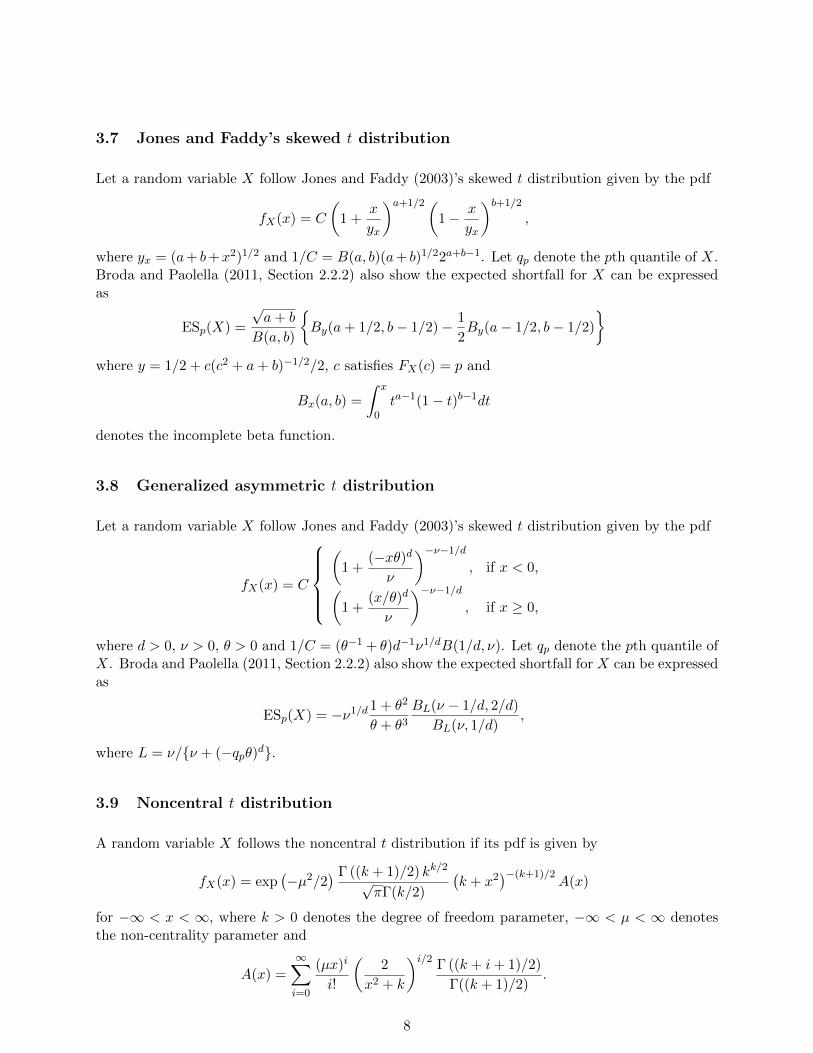
3.7 Jones and Faddy’s skewed t distribution
Let a random variable X follow Jones and Faddy (2003)’s skewed t distribution given by the pdf
fX(x) = C
(1 +
x
yx
)a+1/2(1− x
yx
)b+1/2
,
where yx = (a+ b+x2)1/2 and 1/C = B(a, b)(a+ b)1/22a+b−1. Let qp denote the pth quantile of X.Broda and Paolella (2011, Section 2.2.2) also show the expected shortfall for X can be expressedas
ESp(X) =
√a+ b
B(a, b)
By(a+ 1/2, b− 1/2)− 1
2By(a− 1/2, b− 1/2)
where y = 1/2 + c(c2 + a+ b)−1/2/2, c satisfies FX(c) = p and
Bx(a, b) =
∫ x
0ta−1(1− t)b−1dt
denotes the incomplete beta function.
3.8 Generalized asymmetric t distribution
Let a random variable X follow Jones and Faddy (2003)’s skewed t distribution given by the pdf
fX(x) = C
(
1 +(−xθ)d
ν
)−ν−1/d, if x < 0,(
1 +(x/θ)d
ν
)−ν−1/d, if x ≥ 0,
where d > 0, ν > 0, θ > 0 and 1/C = (θ−1 + θ)d−1ν1/dB(1/d, ν). Let qp denote the pth quantile ofX. Broda and Paolella (2011, Section 2.2.2) also show the expected shortfall for X can be expressedas
ESp(X) = −ν1/d 1 + θ2
θ + θ3BL(ν − 1/d, 2/d)
BL(ν, 1/d),
where L = ν/ν + (−qpθ)d.
3.9 Noncentral t distribution
A random variable X follows the noncentral t distribution if its pdf is given by
fX(x) = exp(−µ2/2
) Γ ((k + 1)/2) kk/2√πΓ(k/2)
(k + x2
)−(k+1)/2A(x)
for −∞ < x < ∞, where k > 0 denotes the degree of freedom parameter, −∞ < µ < ∞ denotesthe non-centrality parameter and
A(x) =∞∑i=0
(µx)i
i!
(2
x2 + k
)i/2 Γ ((k + i+ 1)/2)
Γ((k + 1)/2).
8

Broda and Paolella (2011, Section 2.2.2) also show the expected shortfall for X can be expressedas
ESp(X) = exp(−µ2/2
) Γ ((k + 1)/2) kk/2√πΓ(k/2)
∫ q
−∞x(k + x2
)−(k+1)/2A(x)dx
for q satisfying FX(c) = p. The noncentral t distribution has received much applications in riskmanagement since the paper by Harvey and Siddique (1999).
3.10 Stable distribution
A random variable, say S, is said to have stable distribution with tail index parameter 1 < α ≤ 2and asymmetry parameter β ∈ [−1, 1] if its characteristic function is given by
lnφX(t) = −|t|α[1− iβsign(t) tan
πα
2
],
where i =√−1 is the imaginary unit. We write S ∼ Sα,β(0, 1). Let X denote the location-scale
variant X = µ+ σS and let qp = F−1S (p) denote the pth quantile of S. Broda and Paolella (2011,Section 2.2.3) also show the expected shortfall for X can be expressed as
ESp(X) =1
pStoy (qp, α, β) ,
where
Stoy(c, α, β) =α
α− 1
| c |π
∫ π/2
−θ0g(θ) exp
− | c |α/(α−1) v(θ)
dθ,
g(θ) =sinα(θ0 + θ
)− 2θ
sinα(θ0 + θ
) − α cos2 θ
sin2α(θ0 + θ
) ,v(θ) =
cos(αθ0)1/(α−1) [ cos θ
sinα(θ0 + θ
)]α/(α−1) cosα(θ0 + θ
)− θ
cos θ,
θ0 =1
αarctan
β tan
(πα2
), β = sign(c)β.
3.11 Generalized hyperbolic distribution
A random variable X follows the generalized hyperbolic distribution if its has the pdf
fX(x) =(η/δ)λ√
2πKλ(δη)
Kλ−1/2
(α√δ2 + (x− µ)2
)√
δ2 + (x− µ)2/α1/2−λ exp [β(x− µ)] ,
where µ ∈ R is the location parameter, α ∈ R is the shape parameter, β ∈ R is the asymmetryparameter, δ ∈ R is the scale parameter, λ ∈ R, η =
√α2 − β2, and Kν(·) is the modified Bessel
9

function of order ν. Broda and Paolella (2011, Section 2.2.4) also show the expected shortfall forX can be expressed as
ESp(X) =(η/δ)λ√
2πKλ(δη)
∫ q
−∞xKλ−1/2
(α√δ2 + (x− µ)2
)√
δ2 + (x− µ)2/α1/2−λ exp [β(x− µ)] dx
for q satisfying FX(c) = p.
3.12 Normal mixture distribution
Broda and Paolella (2011, Section 2.3.2) also derive a formula for expected shortfall for a k-component normal mixture. Let X denote a random variable with the cdf
FX(x) =k∑i=1
λiΦ
(x− µiσi
),
where λi are non-negative weights summing to one, −∞ < µi <∞ and σi > 0, where Φ(·) denotesthe standard normal cdf. Let qp denote the quantile defined by FX(qp) = p and let cj = (qp−µj)/σj .Broda and Paolella (2011, Section 2.3.2) show that the expected shortfall of X can be expressed as
ESp(X) =k∑i=1
λiΦ (ci)
p
µi − σi
φ (ci)
Φ (ci)
.
3.13 Stable mixture distribution
Let a random variable X represent a k-component normal mixture of symmetric stable randomvariables with non-negative weights λj , location parameters µj , scale parameters σj and zero asym-metry parameters. Let qp denote the pth quantile of X and let cj = (qp − µj)/σj . Broda andPaolella (2011, Section 2.3.3) also show that the expected shortfall of X can be expressed as
ESp(X) =1
p
k∑i=1
λi [σiStoy (ci, αi) + µiFS (ci)] ,
where S ∼ Sα,0(0, 1).
3.14 Student’s t mixture distribution
Let a random variable X represent a k-component normal mixture of Student’s t random variableswith non-negative weights λj , location parameters µj , scale parameters σj and degrees of freedomνj . Let qp denote the pth quantile of X and let cj = (qp−µj)/σj . Broda and Paolella (2011, Section2.3.4) also show that the expected shortfall of X can be expressed as
ESp(X) =1
p
k∑i=1
λi
[σiTtail (ci, νi) +
µiν−1/2i
B (νi/2, 1/2)
∫ ci
−∞
(1 +
x2
νi
)−(νi+1)/2
dx
].
10

3.15 Generalized Pareto distribution
Suppose the financial observations of interest, say X1, X2, . . . , Xn, follow the generalized Paretodistribution given by the cdf
F (x) = 1−
1 + ξx− uσ
−1/ξ,
where either u < x < ∞ (ξ ≥ 0) or u < x < u− σ/ξ (ξ < 0). In this case, Pattarathammas et al.(2008) show that the expected shortfall can be expressed as
ESp(X) =1
1− ξ
u+
σ
ξ
[n(1− p)Nu
−ξ− 1
]+β − ξu1− ξ
where Nu is the number of observations exceeding u. An estimate of ESp(X) can be obtained byreplacing the parameters, ξ and σ, by their maximum likelihood estimators.
3.16 Asymmetric exponential power distribution
A random variable X is said to have the asymmetric exponential power distribution if its pdf isgiven by
f(x) =
α
α∗K (p1) exp
[− 1
p1
∣∣∣ x2α∗
∣∣∣p1] , if x ≤ 0,
1− α1− α∗
K (p2) exp
[− 1
p2
∣∣∣∣ x
2 (1− α∗)
∣∣∣∣p2] , if x > 0,
where 0 < α < 1 is the skewness parameter, p1 > 0, p2 > 0, K(v) = 1/[2p1/pΓ(1 + 1/p)],α∗ = αK(p1)/[αK(p1) + (1− α)K(p2)], and
α
α∗K (p1) =
1− α1− α∗
K (p2) = αK (p1) + (1− α)K (p2) = B.
For a standard asymmetric exponential power random variable, Zhu and Galbraith (2011) haveshown that the expected shortfall of X is given by
ESp(X) =2
F (q)
− αα∗E (p1)
[1−G
(h1(q),
2
p1
)]
+ (1− α) (1− α∗)E (p2)G
(h2(q),
2
p2
),
where F (·) denotes the cdf of X, q is the root of F (q) = p, and
E(p) = p1/pΓ(2/p)/Γ(1/p),
G(x, a) = γ(a, x)/Γ(a),
h1(q) =1
p1
∣∣∣∣min(q, 0)
2α∗
∣∣∣∣p1 , h1(q) =1
p2
∣∣∣∣max(q, 0)
2 (1− α∗)
∣∣∣∣p2 ,where γ(a, x) =
∫ x0 t
a−1 exp(−t)dt denotes the incomplete gamma function.
11
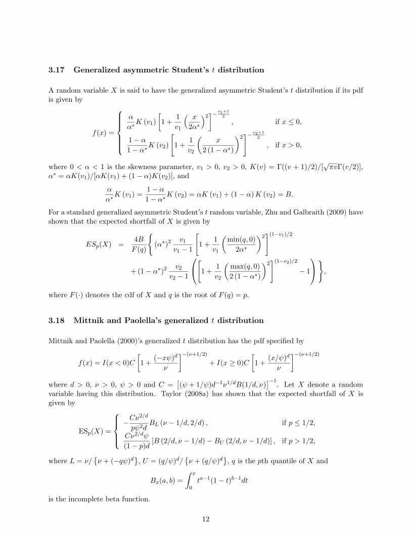
3.17 Generalized asymmetric Student’s t distribution
A random variable X is said to have the generalized asymmetric Student’s t distribution if its pdfis given by
f(x) =
α
α∗K (v1)
[1 +
1
v1
( x
2α∗
)2]− v1+12
, if x ≤ 0,
1− α1− α∗
K (v2)
[1 +
1
v2
(x
2 (1− α∗)
)2]− v2+1
2
, if x > 0,
where 0 < α < 1 is the skewness parameter, v1 > 0, v2 > 0, K(v) = Γ((v + 1)/2)/[√πvΓ(v/2)],
α∗ = αK(v1)/[αK(v1) + (1− α)K(v2)], and
α
α∗K (v1) =
1− α1− α∗
K (v2) = αK (v1) + (1− α)K (v2) = B.
For a standard generalized asymmetric Student’s t random variable, Zhu and Galbraith (2009) haveshown that the expected shortfall of X is given by
ESp(X) =4B
F (q)
(α∗)2
v1v1 − 1
[1 +
1
v1
(min(q, 0)
2α∗
)2](1−v1)/2
+ (1− α∗)2 v2v2 − 1
[1 +1
v2
(max(q, 0)
2 (1− α∗)
)2](1−v2)/2
− 1
,where F (·) denotes the cdf of X and q is the root of F (q) = p.
3.18 Mittnik and Paolella’s generalized t distribution
Mittnik and Paolella (2000)’s generalized t distribution has the pdf specified by
f(x) = I(x < 0)C
[1 +
(−xψ)d
ν
]−(ν+1/2)
+ I(x ≥ 0)C
[1 +
(x/ψ)d
ν
]−(ν+1/2)
where d > 0, ν > 0, ψ > 0 and C =[(ψ + 1/ψ)d−1ν1/dB(1/d, ν)
]−1. Let X denote a random
variable having this distribution. Taylor (2008a) has shown that the expected shortfall of X isgiven by
ESp(X) =
−Cν
2/d
pψ2dBL (ν − 1/d, 2/d) , if p ≤ 1/2,
Cν2/dψ
(1− p)d[B (2/d, ν − 1/d)−BU (2/d, ν − 1/d)] , if p > 1/2,
where L = ν/ν + (−qψ)d
, U = (q/ψ)d/
ν + (q/ψ)d
, q is the pth quantile of X and
Bx(a, b) =
∫ x
0ta−1(1− t)b−1dt
is the incomplete beta function.
12

3.19 Asymmetric Laplace distribution
Lu et al. (2010)’s asymmetric Laplace distribution has the pdf specified by
f(x) =b
τexp
[− bτ| x− τ |
(1
cI(x < γ) +
1
1− cI(x > γ)
)],
where b =√c2 + (1− c)2, γ is a location parameter, τ is a scale parameter, and c is a shape
parameter. Let X denote a random variable having this pdf. Chen et al. (2012) have shown thatthe expected shortfall of X is given by
ESp =c
b
[ln(pc
]− 1]
for 0 ≤ p < c.
3.20 Elliptical distribution
Suppose a portfolio loss can be expressed as X = δ1X1 + · · · + δnXn = δTX, where δi are non-negative weights summing to one, Xi are assets losses, δ = (δ1, . . . , δn), and X = (X1, . . . , Xn). Sup-
pose too that X has the elliptical distribution given by the pdf f(x) =| Σ |−1 g(
(x− µ)T Σ−1 (x− µ))
.
In this case, Kamdem (2005) shows that the expected shortfall of X can be expressed as
ESp(X) = −δµ +∣∣δTΣδ
∣∣1/2 π(n−1)/2
pΓ ((n+ 1)/2)
∫ ∞q2
(u− q2
)(n−1)/2g(u)du, (6)
where q is the root of
π(n−1)/2
Γ ((n+ 1)/2)
∫ ∞q
∫ ∞z
(u− z)(n−3)/2g(u)dudz = p.
The multivariate t distribution mean vector µ, covariance matrix Σ and degrees of freedom νis a member of the elliptical family. For this particular case, Kamdem (2005) shows that (6) canbe reduced to
ESp(X) = −δµ + a∣∣δTΣδ
∣∣1/2 ,where a is the root of
a =Γ ((ν − 1)/2) νν/2
p√πΓ(ν/2)
(ν + q2
)−(ν+1)/2,
where q is the root of
νν/2Γ ((ν + 1)/2)
ν√πsνΓ(ν/2)
2F1
(1 + ν
2,ν
2; 1 +
ν
2;− ν
s2
)= p,
where 2F1(a, b; c;x) denotes the Gauss hypergeometric function.
13

3.21 Multivariate gamma distribution
Suppose a portfolio loss can be expressed as S = X1+ · · ·+Xn, where Xi are assets losses. Supposetoo that (X1, . . . , Xn) has Mathai and Moschopoulos (1991)’s multivariate gamma distribution;that is,
Xj =α0
αjY0 + Yj
for j = 1, 2, . . . , n, where Yj , j = 0, 1, . . . , n are independent gamma random variables with shapeparameters γj and scale parameters αj . According to Mathai and Moschopoulos (1991, Theorem2.1), the pdf of S can be expressed as
fS(s) =∞∑k=0
pkg (s|γ + k, αmax) ,
where αmax = max(α1, . . . , αn), γ = γ1 + · · ·+ γn, pk = Cδk, k = 0, 1, . . ., where
C =n∏j=1
(αjαmax
)γj,
∆j,i =
(1− αj
αmax
)i, j = 1, 2, . . . , n, i = 1, 2, . . . , k,
δk = k−1k∑i=1
n∑j=1
γj∆j,iδk−i, k > 0
and δ0 = 1. The cdf of S is a gamma random variable with shape parameter γ + K and scaleparameter αmax, where K is a discrete random variable with pmf pk = Cδk, k = 0, 1, . . ..
Furman and Landsman (2005) derive an expression for the expected shortfall of S. Let V anindependent convolution of a gamma random variable with shape parameter γ + K + 1 and scaleparameter αmax and another gamma random variable with shape parameter γ0 and scale parameterα0/η. Let Zt, t = 0, 1, . . . , n denote a gamma random variable with unit shape parameter and scaleparameter αt. Let Zmax denote the Zt for which αt = max(α0, αmax). Further, let EK(·) and EV (·)denote the expectations with respect to K and V , respectively. Then, according to Furman andLandsman (2005, Theorem 1), the expected shortfall of S can be expressed as
ESp(S) = ηγ0α0
1− FS+ηZ0 (sp)
1− FS (sp)+
γ
αmax
1− FS+Zmax (sp)
1− FS (sp)
+EK
(KEV
(Γ−1 (γ +K + V + 1) γ (γ +K + V + 1, αmax)
))αmaxFS (sp)
,
where sp satisfies FS(sp) = p and γ(a, x) =∫ x0 t
a−1 exp(−t)dt denotes the incomplete gammafunction.
3.22 Bayesian approach
Let X1, X2, . . . , Xn denote the financial series of interest and let PL(·) denote the profit and lossfunction associated with the series. Suppose the series is fitted to a model parameterized by θ,
14
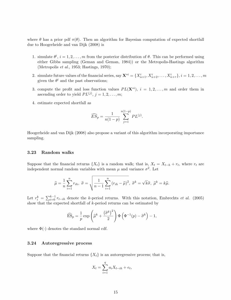
where θ has a prior pdf π(θ). Then an algorithm for Bayesian computation of expected shortfalldue to Hoogerheide and van Dijk (2008) is
1. simulate θi, i = 1, 2, . . . ,m from the posterior distribution of θ. This can be performed usingeither Gibbs sampling (Geman and Geman, 1984)) or the Metropolis-Hastings algorithm(Metropolis et al., 1953; Hastings, 1970);
2. simulate future values of the financial series, say X∗i = Xin+1, X
in+2, . . . , X
in+τ, i = 1, 2, . . . ,m
given the θi and the past observations;
3. compute the profit and loss function values PL(X∗i), i = 1, 2, . . . ,m and order them inascending order to yield PL(j), j = 1, 2, . . . ,m;
4. estimate expected shortfall as
ESp =1
n(1− p)
n(1−p)∑j=1
PL(j).
Hoogerheide and van Dijk (2008) also propose a variant of this algorithm incorporating importancesampling.
3.23 Random walks
Suppose that the financial returns Xt is a random walk; that is, Xt = Xt−h + rt, where rt areindependent normal random variables with mean µ and variance σ2. Let
µ =1
n
n∑i=1
rih, σ =
√√√√ 1
n− 1
n∑i=1
(rih − µ)2, σk =√kσ, µk = kµ.
Let rki =∑k−1
i=0 rt−ih denote the k-period returns. With this notation, Embrechts et al. (2005)show that the expected shortfall of k-period returns can be estimated by
ESp =1
pexp
(µk +
(σk)2
2
)Φ(
Φ−1(p)− σk)− 1,
where Φ(·) denotes the standard normal cdf.
3.24 Autoregressive process
Suppose that the financial returns Xt is an autoregressive process; that is,
Xt =
q∑i=1
aiXt−ih + et,
15
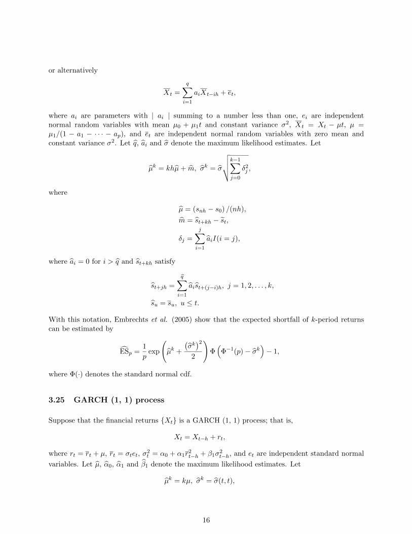
or alternatively
Xt =
q∑i=1
aiXt−ih + et,
where ai are parameters with | ai | summing to a number less than one, ei are independentnormal random variables with mean µ0 + µ1t and constant variance σ2, Xt = Xt − µt, µ =µ1/(1 − a1 − · · · − ap), and et are independent normal random variables with zero mean andconstant variance σ2. Let q, ai and σ denote the maximum likelihood estimates. Let
µk = khµ+ m, σk = σ
√√√√k−1∑j=0
δ2j ,
where
µ = (snh − s0) /(nh),
m = st+kh − st,
δj =
j∑i=1
aiI(i = j),
where ai = 0 for i > q and st+kh satisfy
st+jh =
q∑i=1
aist+(j−i)h, j = 1, 2, . . . , k,
su = su, u ≤ t.
With this notation, Embrechts et al. (2005) show that the expected shortfall of k-period returnscan be estimated by
ESp =1
pexp
(µk +
(σk)2
2
)Φ(
Φ−1(p)− σk)− 1,
where Φ(·) denotes the standard normal cdf.
3.25 GARCH (1, 1) process
Suppose that the financial returns Xt is a GARCH (1, 1) process; that is,
Xt = Xt−h + rt,
where rt = rt + µ, rt = σtet, σ2t = α0 + α1r
2t−h + β1σ
2t−h, and et are independent standard normal
variables. Let µ, α0, α1 and β1 denote the maximum likelihood estimates. Let
µk = kµ, σk = σ(t, t),
16
where σ(t, t) is specified by
σ2 (t∗, t) = α0 + α1
(rkt∗ − µk
)2+ β1σ
2 (t∗ − kh, t) ,
σ2 (t− nkh, t) =k
nk − 1
nk−1∑i=0
(rt−ih − µ)2
for t∗ = t − (n − 1)kh, . . . , t − kh, t and n denoting the number of k-period returns. With thisnotation, Embrechts et al. (2005) show that the expected shortfall of k-period returns can beestimated by
ESp =1
p
∫ p
0exp
(µk + σkxq
νk
)dq − 1,
where xqν denotes the qth quantile of a Student’s t random variable with ν degrees of freedom andµk is calculated using a six-step procedure described in Section 5 of Embrechts et al. (2005).
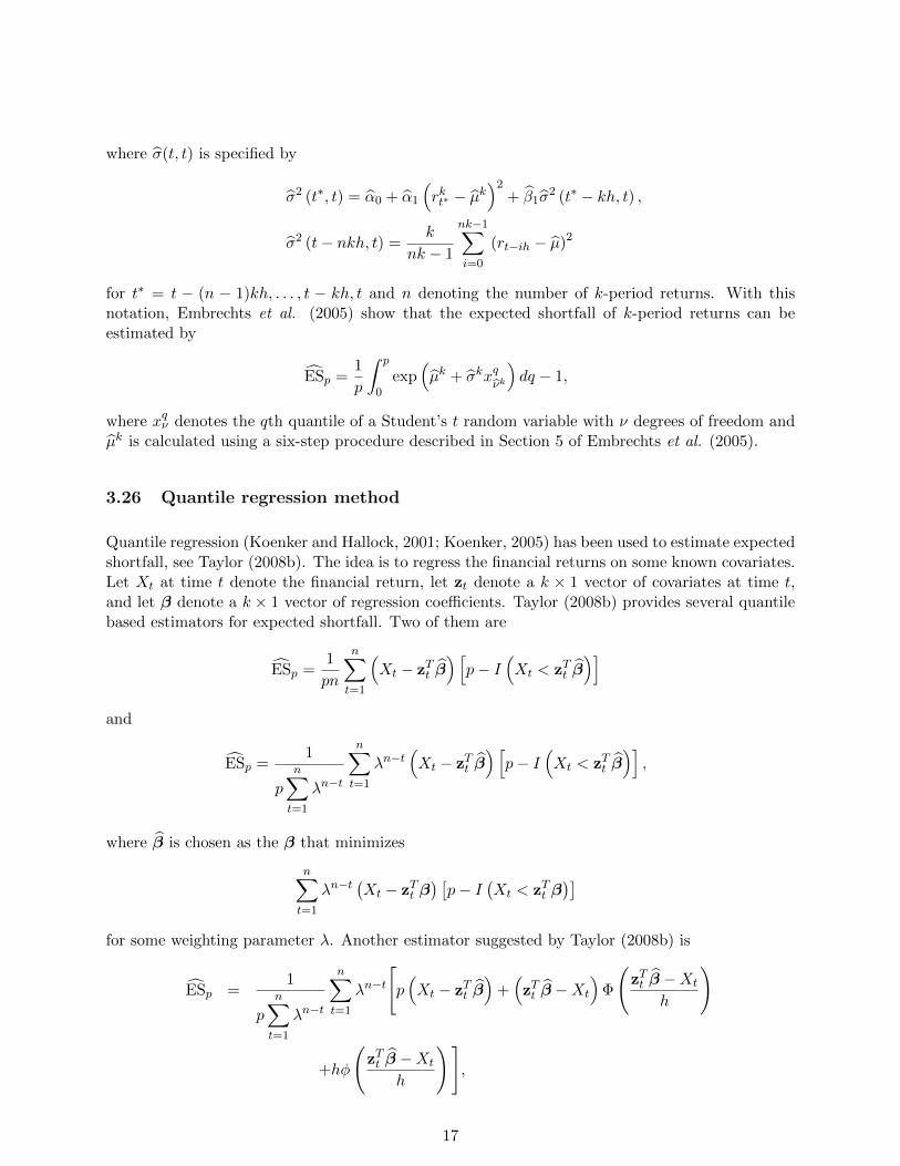
3.26 Quantile regression method
Quantile regression (Koenker and Hallock, 2001; Koenker, 2005) has been used to estimate expectedshortfall, see Taylor (2008b). The idea is to regress the financial returns on some known covariates.Let Xt at time t denote the financial return, let zt denote a k × 1 vector of covariates at time t,and let β denote a k × 1 vector of regression coefficients. Taylor (2008b) provides several quantilebased estimators for expected shortfall. Two of them are
ESp =1
pn
n∑t=1
(Xt − zTt β
) [p− I
(Xt < zTt β
)]and
ESp =1
pn∑t=1
λn−t
n∑t=1
λn−t(Xt − zTt β
) [p− I
(Xt < zTt β
)],
where β is chosen as the β that minimizes
n∑t=1
λn−t(Xt − zTt β
) [p− I
(Xt < zTt β
)]for some weighting parameter λ. Another estimator suggested by Taylor (2008b) is
ESp =1
p
n∑t=1
λn−t
n∑t=1
λn−t
[p(Xt − zTt β
)+(zTt β −Xt
)Φ
(zTt β −Xt
h
)
+hφ
(zTt β −Xt
h
)],
17
where β is chosen as the β that minimizes
n∑t=1
λn−t
[p(Xt − zTt β
)+(zTt β −Xt
)Φ
(zTt β −Xt
h
)+ hφ
(zTt β −Xt
h
)]
for some weighting parameter λ and a suitable bandwidth h.
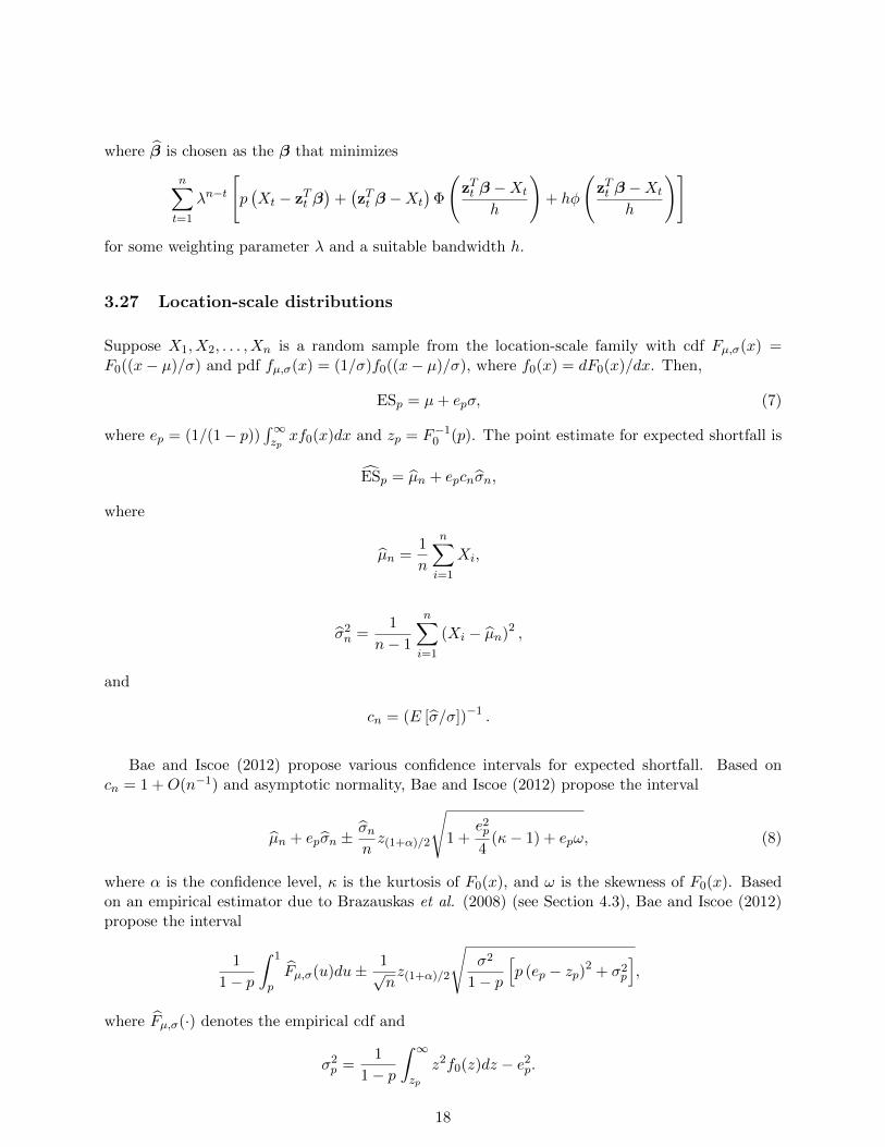
3.27 Location-scale distributions
Suppose X1, X2, . . . , Xn is a random sample from the location-scale family with cdf Fµ,σ(x) =F0((x− µ)/σ) and pdf fµ,σ(x) = (1/σ)f0((x− µ)/σ), where f0(x) = dF0(x)/dx. Then,
ESp = µ+ epσ, (7)
where ep = (1/(1− p))∫∞zpxf0(x)dx and zp = F−10 (p). The point estimate for expected shortfall is
ESp = µn + epcnσn,
where
µn =1
n
n∑i=1
Xi,
σ2n =1
n− 1
n∑i=1
(Xi − µn)2 ,
and
cn = (E [σ/σ])−1 .
Bae and Iscoe (2012) propose various confidence intervals for expected shortfall. Based oncn = 1 +O(n−1) and asymptotic normality, Bae and Iscoe (2012) propose the interval
µn + epσn ±σnnz(1+α)/2
√1 +
e2p4
(κ− 1) + epω, (8)
where α is the confidence level, κ is the kurtosis of F0(x), and ω is the skewness of F0(x). Basedon an empirical estimator due to Brazauskas et al. (2008) (see Section 4.3), Bae and Iscoe (2012)propose the interval
1
1− p
∫ 1
pFµ,σ(u)du± 1√
nz(1+α)/2
√σ2
1− p
[p (ep − zp)2 + σ2p
],
where Fµ,σ(·) denotes the empirical cdf and
σ2p =1
1− p
∫ ∞zp
z2f0(z)dz − e2p.
18

Sometimes the financial series of interest is strictly positive. In this case, if X1, X2, . . . , Xn isa random sample from a log location-scale family with distribution function Gµ,σ(x) = lnF0((x −µ)/σ), then (7) and (8) will generalize to
ESp = exp (µ+ hp(σ))
and
exp
µn + hp (σn)± σn√nz(1+α)/2
√1 +
ν2p (σn)
4(κ− 1) + νp (σn)ω
,respectively, as noted by Bae and Iscoe (2012), where
hp(y) = ln
[1
1− p
∫ ∞zp
exp(ty)f0(t)dt
]
and
νp(σ) =
∫ ∞zp
t exp(σt)f0(t)dt∫ ∞zp
exp(σt)f0(t)dt
.
3.28 RiskMetrics model
Let rt be the financial return at time t and let Ωt denote the information available up to time t.Then the aggregate return from time t to time t+h is rt+1 + · · ·+rt+h = Rt,h say. The RiskMetricsmodel (RiskMetrics Group, 1996) supposes Rt,h | Ωt is normal with mean hµ and variance hσ2t+1,where µ = E(rt+1 | Ωt) and σ2t+1 = V ar(rt+1 | Ωt). So, the corresponding expected shortfall is
ESp = hµ−√h
pσt+1φ
(Φ−1(p)
),
where φ(·) denotes the standard normal pdf and Φ(·) denotes the standard normal cdf.
3.29 QGARCH (1, 1) model
With the notation as in Section 3.28, suppose Rt,h | Ωt is normal with mean hµ and varianceV ar(Rt,h | Ωt) unspecified. In this case, one has the QGARCH (1, 1) model (Wong and So, 2010)with the corresponding expected shortfall given by
ESp = hµ−√V ar (Rt,h | Ωt)
pφ(Φ−1(p)
),
where φ(·) denotes the standard normal pdf and Φ(·) denotes the standard normal cdf.
19
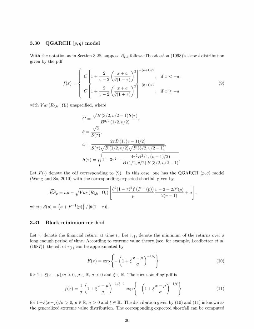
3.30 QGARCH (p, q) model
With the notation as in Section 3.28, suppose Rt,h follows Theodossiou (1998)’s skew t distributiongiven by the pdf
f(x) =
C
[1 +
2
v − 2
(x+ a
θ(1− τ)
)2]−(v+1)/2
, if x < −a,
C
[1 +
2
v − 2
(x+ a
θ(1 + τ)
)2]−(v+1)/2
, if x ≥ −a
(9)
with V ar(Rt,h | Ωt) unspecified, where
C =
√B (3/2, v/2− 1)S(τ)
B3/2 (1/2, v/2),
θ =
√2
S(τ),
a =2τB (1, (v − 1)/2)
S(τ)√B (1/2, v/2)
√B (3/2, v/2− 1)
,
S(τ) =
√1 + 3τ2 − 4τ2B2 (1, (v − 1)/2)
B (1/2, v/2)B (3/2, v/2− 1).
Let F (·) denote the cdf corresponding to (9). In this case, one has the QGARCH (p, q) model(Wong and So, 2010) with the corresponding expected shortfall given by
ESp = hµ−√V ar (Rt,h | Ωt)
[θ2(1− τ)2f
(F−1(p)
)p
v − 2 + 2β2(p)
2(v − 1)+ a
],
where β(p) =a+ F−1(p)
/ [θ(1− τ)].
3.31 Block minimum method
Let rt denote the financial return at time t. Let r(1) denote the minimum of the returns over along enough period of time. According to extreme value theory (see, for example, Leadbetter et al.(1987)), the cdf of r(1) can be approximated by
F (x) = exp
−(
1 + ξx− µσ
)−1/ξ(10)
for 1 + ξ(x− µ)/σ > 0, µ ∈ R, σ > 0 and ξ ∈ R. The corresponding pdf is
f(x) =1
σ
(1 + ξ
x− µσ
)−1/ξ−1exp
−(
1 + ξx− µσ
)−1/ξ(11)
for 1+ξ(x−µ)/σ > 0, µ ∈ R, σ > 0 and ξ ∈ R. The distribution given by (10) and (11) is known asthe generalized extreme value distribution. The corresponding expected shortfall can be computed
20

as
ESp =1
σ
∫ u
−∞x
(1 + ξ
x− µσ
)−1/ξ−1exp
−(
1 + ξx− µσ
)−1/ξdx,
where
u = µ− σ
ξ
[1− − ln p−ξ
]. (12)
See Ou and Yi (2009).
4 Nonparametric methods
4.1 Historical method
Let X(1) ≤ X(2) ≤ · · · ≤ X(n) denote the order statistics in ascending order corresponding tothe original financial returns X1, X2, . . . , Xn. The historical method suggests to estimate expectedshortfall by
ESp(X) =
n∑i=[np]
X(i)
/(n− [np]),
where [x] denotes the largest integer not greater than x.
4.2 Filtered historical method
Let ei, i = 1, 2, . . . , n denote the residuals after the financial series is fitted to some model likeARMA-GARCH. Then the filtered historical estimator of expected shortfall (Magadia, 2011) isgiven by
ESp(X) =
∑ηt>q
ηt∑ηt>q
Iηt>q,
where
ηt = et −1
n
n∑t=1
et
and q = η([pn]+1) is the ([pn] + 1)th order statistic of η1, . . . , ηn.
4.3 Brazauskas et al.’s estimator
For the financial series in Section 4.1, let F (·) denote the empirical cdf and F−1(·) its quantilefunction. Brazauskas et al. (2008) suggest the estimator
ESp(X) =1
p
∫ p
0F−1(u)du.
21

4.4 Yamai and Yoshiba’s estimator
With the notation as in Section 4.1, Yamai and Yoshiba (2002) suggest the following estimator forexpected shortfall
ESp(X) =1
n(α− β)
nα∑i=nβ
Xi,
where α is assumed to be much greater than β.
4.5 Inui and Kijima’s estimator
With the notation as in Section 4.1, Inui and Kijima (2005) suggest the following estimator forexpected shortfall
ESp(X) =
−Xk:n, if n(1− p) is an integer,
−pXk:n − (1− p)Xk+1:n, if n(1− p) is not an integer,
where
Xk:n =1
k
(X(1) + · · ·+X(k)
)for k = 1, 2, . . . , n.
4.6 Chen’s estimator
With the notation as in Section 4.1, Chen (2008) suggests the following estimator for expectedshortfall
ESp(X) =1
1 + [np]
n∑i=1
XiI(Xi ≥ X([n(1−p)]+1)
).
4.7 Peracchi and Tanase’s estimator
With the notation as in Section 4.1, Peracchi and Tanase (2008) suggest the following estimatorfor expected shortfall
ESp(X) =1
np
[np]∑i=1
X(i) +
(1− [np]
np
)Y([np]+1).
22

4.8 Jadhav et al.’s estimators
Jadhav et al. (2009) propose several modifications of the historical estimator for expected shortfall.With the notation as in Section 4.1, one estimator proposed is
ESp(X) = −
[np1+a]+1∑i=0
X(i)[np1+a
]+ 2
,
where i =[(n+ 1)p
′
(i)
],
p′
(i) = p− ip
[np] + 1, i = 0, 1, . . . ,
[np1+a
]+ 1,
and a is a constant taking values in [0, 0.1]. Another estimator proposed is
ESp(X) = −
[np1+a]+1∑i=0
(1− hiX(i) + khiXi+1
)[np1+a
]+ 2
,
where i =[(n+ 1)p
′
(i)
], hi = (n+ 1)p
′
(i) −[(n+ 1)p
′
(i)
],
p′
(i) = p− ip
[np] + 1, i = 0, 1, . . . ,
[np1+a
]+ 1,
and a is a constant taking values in [0, 0.1].
4.9 Kernel method
Let X(1) ≤ X(2) ≤ · · · ≤ X(n) denote the order statistics in ascending order corresponding to thefinancial returns X1, X2, . . . , Xn. Let K(·) denote a symmetric kernel, h a suitable bandwidth,Kh(u) = (1/h)K(u/h), A(x) =
∫ x−∞K(u)du and Ah(u) = A(u/h). Yu et al. (2010) suggest the
following formula for kernel estimation of expected shortfall:
ESp(X) =1
np
n∑i=1
XiAh (q(p)−Xi) ,
where
q(p) =
n∑i=1
[∫ i/n
i−1/nKh(t− p)dt
]X(i).
An alternative is to obtain qp as the solution of
1
n
n∑i=1
Ah (x− xi) = p.
Further details on this kernel method can be seen from Scaillet (2004) and Chen (2008).
23
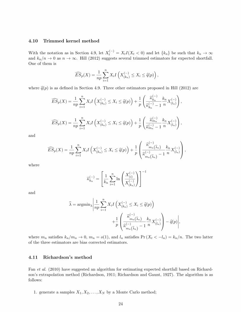
4.10 Trimmed kernel method
With the notation as in Section 4.9, let X(−)t = XtI(Xt < 0) and let kn be such that kn → ∞
and kn/n → 0 as n → ∞. Hill (2012) suggests several trimmed estimators for expected shortfall.One of them is
ESp(X) =1
np
n∑i=1
XiI(X
(−)(kn)≤ Xi ≤ q(p)
),
where q(p) is as defined in Section 4.9. Three other estimators proposed in Hill (2012) are
ESp(X) =1
np
n∑i=1
XiI(X
(−)(kn)≤ Xi ≤ q(p)
)+
1
p
(κ(−)kn
κ(−)kn− 1
knnX
(−)(ln)
),
ESp(X) =1
np
n∑i=1
XiI(X
(−)(kn)≤ Xi ≤ q(p)
)+
1
p
(κ(−)mn
κ(−)mn − 1
knnX
(−)(ln)
),
and
ESp(X) =1
np
n∑i=1
XiI(X
(−)(kn)≤ Xi ≤ q(p)
)+
1
p
κ(−)mn(λn)
κ(−)mn(λn)
− 1
knnX
(−)(ln)
,
where
κ(−)kn
=
1
kn
n∑i=1
ln
X(−)(i)
X(−)(kn)
−1
and
λ = argminλ
∣∣∣∣∣ 1
np
n∑i=1
XiI(X
(−)(kn)≤ Xi ≤ q(p)
)
+1
p
κ(−)mn(λn)
κ(−)mn(λn)
− 1
knnX
(−)(ln)
− q(p)∣∣∣∣∣,where mn satisfies kn/mn → 0, mn = o(1), and ln satisfies Pr (Xt < −ln) = kn/n. The two latterof the three estimators are bias corrected estimators.
4.11 Richardson’s method
Fan et al. (2010) have suggested an algorithm for estimating expected shortfall based on Richard-son’s extrapolation method (Richardson, 1911; Richardson and Gaunt, 1927). The algorithm is asfollows:
1. generate a samples X1, X2, . . . , XN by a Monte Carlo method;
24
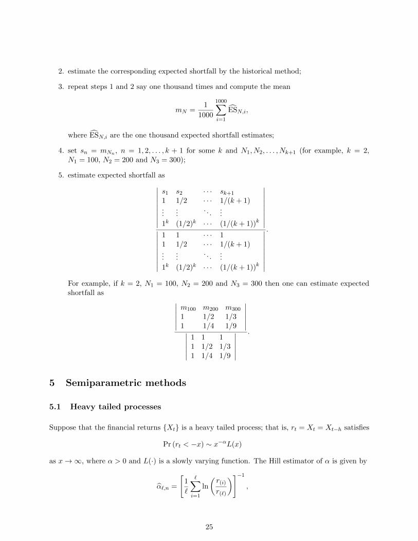
2. estimate the corresponding expected shortfall by the historical method;
3. repeat steps 1 and 2 say one thousand times and compute the mean
mN =1
1000
1000∑i=1
ESN,i,
where ESN,i are the one thousand expected shortfall estimates;
4. set sn = mNn , n = 1, 2, . . . , k + 1 for some k and N1, N2, . . . , Nk+1 (for example, k = 2,N1 = 100, N2 = 200 and N3 = 300);
5. estimate expected shortfall as∣∣∣∣∣∣∣∣∣s1 s2 · · · sk+1
1 1/2 · · · 1/(k + 1)...
.... . .
...
1k (1/2)k · · · (1/(k + 1))k
∣∣∣∣∣∣∣∣∣∣∣∣∣∣∣∣∣∣1 1 · · · 11 1/2 · · · 1/(k + 1)...
.... . .
...
1k (1/2)k · · · (1/(k + 1))k
∣∣∣∣∣∣∣∣∣
.
For example, if k = 2, N1 = 100, N2 = 200 and N3 = 300 then one can estimate expectedshortfall as ∣∣∣∣∣∣
m100 m200 m300
1 1/2 1/31 1/4 1/9
∣∣∣∣∣∣∣∣∣∣∣∣1 1 11 1/2 1/31 1/4 1/9
∣∣∣∣∣∣.
5 Semiparametric methods
5.1 Heavy tailed processes
Suppose that the financial returns Xt is a heavy tailed process; that is, rt = Xt = Xt−h satisfies
Pr (rt < −x) ∼ x−αL(x)
as x→∞, where α > 0 and L(·) is a slowly varying function. The Hill estimator of α is given by
α`,n =
[1
`
∑i=1
ln
(r(i)
r(`)
)]−1,
25

where n denotes the number of k-period returns and r(1) ≤ r(2) ≤ · · · ≤ r(n) are the order statisticsin ascending order. With this notation, Embrechts et al. (2005) show that the expected shortfallof k-period returns can be estimated by
ESp =1
p
∫ p
0exp
[(k`n,pnq
)1/α`n,p,n
r`n,p
]dq − 1,
where `n,p = [n(p+ 0.045 + 0.005h)].
5.2 Necir et al.’s estimator
Let X(1) ≤ X(2) ≤ · · · ≤ X(n) denote the order statistics in ascending order corresponding tothe financial returns X1, X2, . . . , Xn. Another semiparametric estimator for expected shortfallsuggested by Necir et al. (2010) is
ESp =1
p
∫ p
k/nF−1(t)dt+
kX(n−k)
np (1− γ),
where
γ =1
k
k∑i=1
lnX(n−i+1)
X(n−k)
is Hill’s estimator of tail index and F−1(·) denotes the empirical quantile function.
6 Computer software
Software for computing expected shortfall and related quantities are widely available. Some softwareavailable from the R package (R Development Core Team, 2011) are:
• the package ghyp due to David Luethi, Wolfgang Breymann. According to the author, thispackage “provides detailed functionality for working with the univariate and multivariateGeneralized Hyperbolic distribution and its special cases (Hyperbolic (hyp), Normal InverseGaussian (NIG), Variance Gamma (VG), skewed Student-t and Gaussian distribution). Es-pecially, it contains fitting procedures, an AIC-based model selection routine, and functionsfor the computation of density, quantile, probability, random variates, expected shortfall andsome portfolio optimization and plotting routines as well as the likelihood ratio test. Inaddition, it contains the Generalized Inverse Gaussian distribution”;
• the package evir due to Bernhard Pfaff, Alexander McNeil and Alec Stephenson;
• the package fAssets due to the Rmetrics Core Team;
• the package crp.CSFP due to Matthias Fischer, Kevin Jakob and Stefan Kolb;
• the package QRM due to Bernhard Pfaff, Alexander McNeil and Scott Ulmann.
26

Some other software available for computing value at risk and related quantities are:
• the package ALM Optimizer for asset allocation software due to Bob Korkie from the companyRMKorkie & Associates, http://assetallocationsoftware.org/. According to the author, thispackage provides “risk and expected return of Markowitz efficient portfolios but extended toinclude recent technical advances on the definition of risk, adjustments for input bias, nonnormal distributions, and enhancements that allow for overlays, risk budgets, and investmenthorizon adjustments”. Also the package “is a true Portfolio Optimizer with lognormal assetreturns and user specified: return or surplus optimization; optimization, risk, and rebalancinghorizons; volatility, expected shortfall, and two value at risk (VaR) risk variables tailored tothe risk horizon; and user specified portfolio constraints including risk budget constraints”;
• the package QuantLib due to StatPro, http://www.statpro.com/portfolio-analytics-products/risk-management-software/. According to the authors, this package provides “access to a completeuniverse of pricing functions for risk assessment covering every asset class from equity, interestrate-linked products to mortgage-backed securities”. The package has key features including“Multiple ex-ante risk measures including Value-at-Risk and CVaR (expected shortfall) at avariety of confidence levels, potential gain, volatility, tracking error and diversification grade.These measures are available in both absolute and relative basis”;
• the package FinAnalytica’s Cognity risk management due to FinAnalytica, http://www.finanalytica.com/daily-risk-statistics/. According to the authors, this package provide “more accurate fat-tailed VaRestimates that do not suffer from the over-optimism of normal distributions. But Cognitygoes beyond VaR and also provides the downside Expected Tail Loss (ETL) measure - theaverage or expected loss beyond VaR. As compared with volatility and VaR, ETL, also knownas Conditional Value at Risk (CVaR) and Expected Shortfall (ES), is a highly informativeand intuitive measure of extreme downside losses. By combining ETL with fat-tailed distri-butions, risk managers have access to the most accurate estimate of downside risk availabletoday”;
• the package CVaR Expert due to CVaR Expert Rho - Works Advanced Analytical Systems,http://www.rhoworks.com/software/detail/cvarxpert.htm. According to the authors, this pack-age implements “total solution for measuring, analyzing and managing portfolio risk usinghistorical VaR and CVaR methodologies. Traditional Value-at-Risk, Beta VaR, ComponentVaR, Conditional VaR and backtesting modules are incorporated on the current version,which lets you work with individual assets, portfolios, asset groups and multi currency in-vestments (Enterprise Edition). An integrated optimizer can solve for the minimum CVaRportfolio based on market data and investor preferences, offering the best risk benchmarkthat can be produced. A module capable of doing Stochastic Simulation allows you to graphthe CVaR-Return space for all feasible portfolios”;
• the Enterprise Risk Management software (KRM) due to ZSL Inc, http: // www.zsl.com /solutions / banking-finance / enterprise-risk-management-krm. According to the authors, “Ka-makura Risk Manager (KRM) completely integrates credit portfolio management, marketrisk management, asset and liability management, Basel II and other capital allocation tech-nologies, transfer pricing, and performance measurement. KRM is also directly applicableto operational risk, total risk, and accounting and regulatory requirements using the sameanalytical engine, GUI and reporting, and its vision is that completely integrated risk so-lution based on common assumptions and methodologies. KRM offers, dynamic value at
27

risk and expected shortfall, historical value at risk measurement, Monte Carlo value at riskmeasurement, etc”;
• the package NtInsight due to Numerical Technologies Company, http: // www.numtech.com/ news / basel-committee-proposes-expected-shortfall / #more-3396. According to the au-thors, “Numerical Technologies understands the advantages of measuring expected shortfall.NtInsight uses massive parallel programming and applies faster codes when processing thetransaction-level, 1 million Monte Carlo iterations needed to precisely capture the non-linearbehavior of tail risk. It has been tested by major financial institutions in Japan where re-porting expected shortfall is part of the regulatory requirement”;
• the package G@RCH 6, OxMetrics due to Timberlake Consultants Limited, http://www.timberlake.co.uk/?id=64#garch.According to the authors, the package is “dedicated to the estimation and forecasting of uni-variate ARCH-type models. G@RCH provides a user-friendly interface (with rolling menus)as well as some graphical features (through the OxMetrics graphical interface). G@RCH helpsthe financial analysis: value-at-risk, expected shortfall, backtesting (Kupiec LRT, dynamicquantile test); forecasting, realized volatility”.
References
[1] Acerbi, C. and Tasche, D. (2002). On the coherence of expected shortfall. Journal of Bankingand Finance, 26, 1487-1503.
[2] An, S., Sun, J. and Wang, Y. (2005). Research on risk management of basic social securityfund in China. In: Proceedings of the 2005 International Conference on Public Administration,pp. 960-965.
[3] Artzner, P., Delbaen, F., Eber, J. M. and Heath, D. (1997). Thinking coherently. Risk, 10,68-71.
[4] Artzner, P., Delbaen, F., Eber, J. M. and Heath, D. (1999). Coherent measures of risk.Mathematical Finance, 9, 203-228.
[5] Azzalini, A. (1985). A class of distributions which includes the normal ones. ScandinavianJournal of Statistics, 12, 171-178.
[6] Azzalini, A. and Capitanio, A. (2003). Distributions generated by perturbation of symmetrywith emphasis on a multivariate skew t-distribution. Journal of the Royal Statistical Society,B, 65, 367-389.
[7] Bae, T. and Iscoe, I. (2012). Large-sample confidence intervals for risk measures of location-scale families. Journal of Statistical Planning and Inference, 142, 2032-2046.
[8] Bernardi, M. (2012). Risk measures for skew normal mixtures. Working paper, MEMOTEF,Sapienza University of Rome.
[9] Bi, G. and Giles, D. E. (2007). An application of extreme value analysis to US movie box officereturns. In: Proceedings of the 2007: International Congress on Modelling and Simulation:Land, Water and Environmental Management: Integrated Systems for Sustainability, pp.2652-2658.
28
[10] Bi, G. and Giles, D. E. (2009). Modelling the financial risk associated with US movie boxoffice earnings. Mathematics and Computers In Simulation, 79, 2759-2766.
[11] Brazauskas, V., Jones, B., Madan, L. and Zitikis, R. (2008). Estimating conditional tailexpectation with actuarial application in view. Journal of Statistical Planning and Inference,138, 3590-3604.
[12] Broda, S. A. and Paolella, M. S. (2011). Expected shortfall for distributions in finance. In:Statistical Tools for Finance and Insurance, pp. 57-99, Heidelberg, Berlin.
[13] Chen, Q., Gerlach, R. and Lu, Z. (2012). Bayesian Value-at-Risk and expected shortfall fore-casting via the asymmetric Laplace distribution. Computational Statistics and Data Analysis,56, 3498-3516.
[14] Chen, S. X. (2008). Nonparametric estimation of expected shortfall. Journal of FinancialEconometrics, 6, 87-107.
[15] Cheung, K. C. (2009). Upper comonotonicity. Insurance: Mathematics and Economics, 45,35-40.
[16] Cotter, J. and Dowd, K. (2006). Extreme spectral risk measures: An application to futuresclearinghouse margin requirements. Journal of Banking and Finance, 30, 3469-3485.
[17] Embrechts, P., Kaufmann, R. and Patie, P. (2005). Strategic long-term financial risks: singlerisk factors. Computational Optimization and Applications, 32, 61-90.
[18] Fan, G., Wong, W. K. and Zeng, Y. (2008). Backtesting industrial market risks using expectedshortfall: The case of Shanghai stock exchange. In: Proceedings of the 2nd InternationalConference on Management Science and Engineering Management, pp. 413-422.
[19] Fan, G., Zeng, Y. and Wong, W. K. (2010). Risk contribution of different industries in China’sstock market-based on VaR and expected shortfall. In: Proceedings of the 3rd InternationalInstitute of Statistics and Management Engineering Symposium, pp. 526-533.
[20] Fan, G., Zeng, Y. and Wong, W. K. (2012). Decomposition of portfolio VaR and expectedshortfall based on multivariate Copula simulation. International Journal of Management Sci-ence and Engineering Management, 7, 153-160.
[21] Fan, Y., Li, G. and Zhang, M. (2010). Expected shortfall and it’s application in credit riskmeasurement. In: Proceedings of the 2010 Third International Conference on Business Intel-ligence and Financial Engineering, pp. 359-363.
[22] Furman, E. and Landsman, Z. (2005). Risk capital decomposition for a multivariate dependentgamma portfolio. Insurance: Mathematics and Economics, 37, 635-649.
[23] Gao, L. J. and Li, J. P. (2009). The influence of IPO to the operational risk of Chinesecommercial banks. Cutting-Edge Research Topics on Multiple Criteria Decision Making Pro-ceedings, 35, 486-492.
[24] Hafner, R. (2004). Stochastic Implied Volatility. Springer Verlag, Berlin.
[25] Harvey, C. R. and Siddique, A. (1999). Autoregressive conditional skewness. Journal of Fi-nancial and Quantitative Analysis, 34, 465-487.
29

[26] Hill, J. B. (2012). Robust expected shortfall estimation for infinite variance time series.
[27] Hoogerheide, L. F. and van Dijk, H. K. (2008). Bayesian forecasting of value at risk andexpected shortfall using adaptive importance sampling. Tinbergen Institute Discussion Paper,TI 2008-092/4.
[28] Hurlimann, W. (2002). Analytical bounds for two value-at-risk functionals Astin Bulletin,32, 235-265.
[29] Hurlimann, W. (2003). Conditional value-at-risk bounds for compound poisson risks and anormal approximation. Journal of Applied Mathematics, 141-153.
[30] Inui, K. and Kijima, M. (2005). On the significance of expected shortfall as a coherent riskmeasure. Journal of Banking and Finance, 29, 853-864.
[31] Jadhav, D., Ramanathan, T. V. and Naik-Nimbalkar, U. V. (2009). Modified estimators ofthe expected shortfall. Journal of Emerging Market Finance, 8, 87-107.
[32] Johnson, N. L. (1949). System of frequency curves generated by methods of translation.Biometrika, 36, 149-176.
[33] Jones, M. C. and Faddy, M. J. (2003). A skew extension of the t distribution with applications.Journal of the Royal Statistical Society, B, 65, 159-174.
[34] Kamdem, J. S. (2005). Value-at-risk and expected shortfall for linear portfolios with ellipti-cally distributed risk factors. International Journal of Theoretical and Applied Finance, 8,537-551.
[35] Koenker, R. (2005). Quantile Regression. Cambridge University Press, Cambridge.
[36] Koenker, R. and Hallock, K. F. (2001). Quantile regression. Journal of Economic Perspectives,15, 143-156.
[37] Krehbiel, T. and Adkins, L. C. (2008). Extreme daily changes in US Dollar London inter-bankoffer rates. International Review of Economics and Finance, 17, 397-411.
[38] Leadbetter, M. R., Lindgren, G. and Rootzen, H. (1987). Extremes and Related Properties ofRandom Sequences and Processes. Springer Verlag, New York.
[39] Lee, W. C. and Fang, C. J. (2010). The measurement of capital for operational risk in Tai-wanese commercial banks. Journal of Operational Risk, 5, 79-102.
[40] Li, X. M. and Li, F. C. (2006). Extreme value theory: An empirical analysis of equity riskfor Shanghai stock market. In: Proceedings of the 2006 International Conference on ServiceSystems and Service Management, pp. 1073-1077.
[41] Lindstrom, E. and Regland, F. (2012). Modeling extreme dependence between Europeanelectricity markets. Energy Economics, 34, 899-904.
[42] Liu, X. X., Qiu, G. H. and Wu, F. X. (2008). Research of liquidity adjusted VaR and ES inChina stock market based on extreme value theory. In: Proceedings of 2008 China-CanadaIndustry Workshop on Enterprise Risk Management, pp. 377-388.
30
[43] Lu, Z., Huang, H. and Gerlach, R. (2010). Estimating Value at Risk: from JP Morgan’sstandard-EWMA to skewed-EWMA forecasting. University of Sydney Working Paper.
[44] Magadia, J. (2011). Confidence interval for expected shortfall using bootstrap methods.
[45] Mathai, A. M. and Moschopoulos, P. G. (1991). On a multivariate gamma. Journal of Mul-tivariate Analysis, 39, 135-153.
[46] Mittnik, S. and Paolella, M. S. (2000). Conditional density and value-at-risk prediction ofAsian currency exchange rates. Journal of Forecasting, 19, 313-333.
[47] Necir, A., Rassoul, A. and Zitikis, R. (2010). Estimating the conditional tail expectation inthe case of heavy-tailed losses. Journal of Probability and Statistics, Article ID 596839.
[48] Ou, S. and Yi, D. (2009). Robustness analysis and algorithm of expected shortfall based onextreme-value block minimum model. In: Proceedings of the 2009 International Conferenceon Business Intelligence and Financial Engineering, pp. 288-292.
[49] Owen, D. B. (1956). Tables for computing bivariate normal probabilities. Annals of Mathe-matical Statistics, 27, 1075-1090.
[50] Pattarathammas, S., Mokkhavesa, S. and Nilla-Or, P. (2008). Value-at-risk and expectedshortfall under extreme value theory framework: an empirical study on Asian markets.
[51] Peracchi, F. and Tanase, A. V. (2008). On estimating the conditional expected shortfall.Applied Stochastic Models in Business and Industry, 24, 471-493.
[52] R Development Core Team (2011). A Language and Environment for Statistical Computing.R Foundation for Statistical Computing. Vienna, Austria.
[53] Rachev, S., Jasic, T., Stoyanov, S. and Fabozzi, F. J. (2007). Momentum strategies based onreward-risk stock selection criteria. Journal of Banking and Finance, 31, 2325-2346.
[54] Richardson, L. F. (1911). The approximate arithmetical solution by finite differences of physi-cal problems including differential equations, with an application to the stresses in a masonrydam. Philosophical Transactions of the Royal Society of London, A, 210, 307357.
[55] Richardson, L. F. and Gaunt, J. A. (1927). The deferred approach to the limit. PhilosophicalTransactions of the Royal Society of London, A, 226, 299-349.
[56] RiskMetrics Group (1996). RiskMetrics-Technical Document. Morgan J.P.
[57] Scaillet, O. (2004). Nonparametric estimation and sensitivity analysis of expected shortfall.Mathematical Finance, 14, 115-129.
[58] Simonato, J. -G. (2011). The performance of Johnson distributions for computing value atrisk and expected shortfall. Journal of Derivatives, 19, 7-24.
[59] Sims, G. V. and Kamal, I. (1996). Repowering of existing coastal stations to augment watersupplies in Southern California: A study of alternatives. In: Water Supply Puzzle: How doesDesalting Fit In?, pp. 408-429.
[60] Song, J. S., Li, Y., Ji, F. and Peng, C. (2009). Operational risk measurement of Chinesecommercial banks based on extreme value theory. Cutting-Edge Research Topics on MultipleCriteria Decision Making Proceedings, 35, 531-534.
31

[61] Taylor, J. W. (2008a). Estimating value at risk and expected shortfall using expectiles. Journalof Financial Econometrics, 6, 231-252.
[62] Taylor, J. W. (2008b). Using exponentially weighted quantile regression to estimate value atrisk and expected shortfall. Journal of Financial Econometrics, 6, 382-406.
[63] Teng, F. and Zhang, Q. W. (2009). Cash flow risk measurement for Chinese non-life insuranceindustry based on estimation of ES and NRR. In: Proceedings of the 2009 International Forumon Information Technology and Applications, volume 2, pp. 628-631.
[64] Theodossiou, P. (1998). Financial data and the skewed generalized t distribution. ManagementScience, 44, 1650-1661.
[65] Wang, Z. R. and Wu, W. T. (2008). Empirical study for exchange rate risk of CNY: UsingVaR and ES based on extreme value theory. In: Proceedings of the 2008 IEEE InternationalConference on Management of Innovation and Technology, pp. 1193-1198.
[66] Wang, Z. R., Wu, W. T., Chen, C. and Zhou, Y. J. (2010). The exchange rate risk of Chineseyuan: Using VaR and ES based on extreme value theory. Journal of Applied Statistics, 37,265-282.
[67] Wong, C. -M. and So, M. K. P. (2010). On the estimation of multiple period expected shortfalland median shortfall using GARCH models. Quantitative Finance, to appear.
[68] Wuthrich, M. V., Buhlmann, H. and Furrer, H. (2010). Market-consistent Actuarial Valuation,second edition. Springer, Heidelberg.
[69] Yamai, Y. and Yoshiba, T. (2002). Comparative analyses of expected shortfall and value-at-risk: Their estimation error, decomposition, and optimization. Monetary and EconomicStudies, 87-122.
[70] Yu, K., Ally, A. K., Yang, S. and Hand, D. J. (2010). Kernel quantile-based estimation ofexpected shortfall. Journal of Risk, 12, 15-32.
[71] Yu, Z. Y. and Tao, A. Y. (2008). Which one is better? - Risk measurement modeling onChinese stock market. In: Proceedings of the 2008 International Symposium on FinancialEngineering and Risk Management, pp. 47-51.
[72] Zhu, D. and Galbraith, J. W. (2009). Forecasting expected shortfall with a generalized asym-metric Student-t distribution. CIRANO Working Paper.
[73] Zhu, D. and Galbraith, J. W. (2011). Modelling and forecasting expected shortfall with thegeneralized asymmetric Student-t and asymmetric exponential power distributions. Journalof Empirical Finance, 18, 765-778.
32