estimation of load disturbance torque for dc motor drive systems under robustness and sensitivity...

930 IEEE TRANSACTIONS ON INDUSTRIAL ELECTRONICS, VOL. 61, NO. 2, FEBRUARY 2014

Estimation of Load Disturbance Torque for DCMotor Drive Systems Under Robustness and

Sensitivity ConsiderationDanny Grignion, Member, IEEE, Xiang Chen, Member, IEEE, Narayan Kar, Senior Member, IEEE, and Huijie Qian

Abstract—This paper presents multiple methods for the designof a robust disturbance torque estimator. The benefit of thesedesigns is that they ensure robust estimation in the presence ofmodel uncertainties and/or noise. It is shown that these estima-tion schemes can be used to estimate both constant and nearlyconstant disturbance torques. In order to design the observers,the nominal plant model is expanded to incorporate uncertainties.Various cases for the design of the observer are presented. Allof the cases are tested on a real system using varying degrees ofmodel uncertainty to ensure that robust estimation is achieved.The results are validated using an in-line torque sensor and arepresented accordingly.

Index Terms—Disturbance torque estimation, H− index, H∞filtering, multiobjective robust filtering, robust estimation.

NOMENCLATURE

Δ Variation.ωm Motor speed.τd Disturbance torque.τL Load torque.Bm Viscous friction coefficient.ia Armature current.Jm Inertial coefficient.Kt Mechanical constant.Kv Electrical constant.La Armature inductance.Ra Armature resistance.vd Disturbance voltage.vt Armature voltage.

I. INTRODUCTION

D IRECT CURRENT (dc) motors are an important partof many everyday systems. In particular, the automobile

contains an array of dc motors that are used to control variousaspects of the vehicle’s performance and enhance the comfort

Manuscript received June 13, 2012; revised November 13, 2012; acceptedFebruary 14, 2013. Date of publication April 5, 2013; date of current versionAugust 9, 2013. This work was supported in part by the Ontario Research Fundunder the project Green Auto Powertrain, and in part by Natural Science andEngineering Research Council of Canada (NSERC) through Network of Centreof Excellence—Automobile in 21st Century.

The authors are with the Department of Electrical and Computer Engineer-ing, University of Windsor, Windsor, ON N9B 3P4, Canada (e-mail: [email protected]).

Color versions of one or more of the figures in this paper are available onlineat http://ieeexplore.ieee.org.

Digital Object Identifier 10.1109/TIE.2013.2257138

level for the occupants. These applications range from highlysensitive systems, such as electronic throttle control and electricpower steering, to less sensitive systems such as power sunroof,power seats, and power windows. In highly sensitive systems,such as the electronic throttle control system, it is necessary tomaintain as much precision as possible even in the presence ofdisturbance torques that pose themselves on the motor’s shaft.In order to accomplish this task, the system needs to have someknowledge of the disturbance torque.

Due to the difficulty of direct measurement, estimation hasbecome a popular method of measuring the quantity of thedisturbance torque acting on a motor’s shaft. This estimationmay then be used to compensate for the disturbance torqueacting on the shaft, thus improving the system’s robustness toexternal torques and load changes. A well-designed estimationscheme can also be used to reduce the cost of the overall systemas it can be used to estimate other quantities and thus eliminatethe need to use high-priced sensors to measure such quantities.

Three such estimation schemes were presented in [1]. Allof the schemes are based on a Luenberger state observer (see[15] and [16]) that is expanded to incorporate the disturbancetorque in the plant model. This expansion is performed in twoways with the first being that the disturbance torque is treatedas an unknown input and the second being that it is treated asa state variable. This second method was used successfully in[9] and [10]. There is a restriction placed on the design of thistype of estimator in that the disturbance torque acting on theplant is assumed to be constant and only the performance forconstant disturbance torques was shown. It is not guaranteedthat a nonconstant disturbance torque can be estimated.

All of these schemes, though, do not incorporate the presenceof model uncertainties into the design of the estimator. Anobserver design that also takes into account these uncertaintieswould serve not only to provide a good estimation but also torobustify the estimation to variations in the parameters of theplant. Two such filters are the H∞ filter discussed in [22] and[26] and the H∞-Gaussian filter in [3] and [4]. These filtersare designed to provide a robust estimate in the presence ofmodel uncertainties (and noise in the case of the H∞-Gaussianfilter). This is achieved through the solution of two coupledalgebraic Riccati equations (AREs). Another example of thistype of estimation can be found in [25]. A brief descriptionof these designs will be discussed later in this paper. It shouldbe noted that these designs are not the only methods availableto design an observer or to estimate a disturbance. For otherdesigns, see [2], [5], [6]–[8], [18], [19]–[21], [23], and [24].

0278-0046 © 2013 IEEE

GRIGNION et al.: ESTIMATION OF LOAD DISTURBANCE TORQUE FOR DC MOTOR DRIVE SYSTEMS 931

It can be shown that the error dynamics of the systemare affected not only by model uncertainties but also by thedisturbance acting on the system and that the disturbance torqueestimation is proportional to the error in the estimation of themotor’s armature current. This raises an interesting question asto how an estimator design can be conducted that maximizes thesensitivity of the error to the disturbance to be estimated whileminimizing the sensitivity of the error to model uncertainties.A good filter design will make a tradeoff between these twoconflicting requirements. In order to facilitate such a design,a second measure is needed in order to properly gauge thesensitivity to a disturbance.

The H− index can be used for such a purpose. This indexcan be used to achieve the desired sensitivity to disturbanceby maximizing the H− index of the transfer function fromdisturbance to error. A mix of these two measures would thusprovide a means for achieving such a filter design. One suchdesign is the multiobjective H−/H∞ filter, presented in [11]–[14], that has been used for fault detection.

This paper will use an H∞ filter, an H∞-Gaussian filter, and amultiobjective H−/H∞ filter as the basis for three disturbancetorque estimator designs. The filters will be used to estimatethe disturbance torque acting on the motor shaft, without anyprior knowledge or model of the disturbance itself, and in thepresence of model uncertainty. The aim of this is to ensure thatthe design of the observer and the estimate which it producesare robust to model uncertainties and/or noise.

This paper is organized as follows. Section II will providethe definitions of the H∞ norm, H2 norm, and H− index anda brief theoretical background of a generic observer and filterdesigns and also discusses the modeling of a dc motor drive sys-tem. Section III discusses the design of the disturbance torqueestimators. Section IV presents some test results. Section Vconcludes this paper.

II. MODELING AND BACKGROUND THEORY

A. Notations and Definitions

The following notations and definitions are used throughoutthis paper (see [3], [4], [11]–[14], [22], [26], and [27]). Matricesand vectors are represented using bold lettering.ˆdenotes anestimated state variable, and ˙ denotes a derivative with respectto time. If A is a matrix or vector, then AT and A∗ denote itstranspose and conjugate transpose, respectively. I and 0 denotean identity matrix of appropriate dimensions and a zero matrixof appropriate dimensions, respectively. σ(A) and σ(A) denotethe largest and smallest singular values of A, respectively.

Let G(s) be a proper real rational transfer matrix. A state-space realization of G(s) is

G(s) =

[A B

C D

]= C(sI −A)−1B +D.

A left coprime factorization (LCF) of G(s) is a factorizationG(s) = M−1(s)N(s) where M(s) and N(s) are left coprimeover G(s) ∈ RH∞ and RH∞ is the space of all proper andreal rational stable matrix transfer functions. Let the state-spacerealization of G(s) above be detectable, and let L be a matrix

with appropriate dimensions such that A+LC is stable. Then,an LCF of G(s) is given by

[M(s) N(s)] =

[A+LC L B +LD

C I D

].

For G(s) ∈ RH2 where RH2 is the space of all strictlyproper and real rational stable matrix transfer functions, the H2

norm of G(s) is defined as

‖G(s)2‖ =

√√√√√ 1

2π

∞∫−∞

trace [G∗(jω)G(jω)] dω.

For G(s) ∈ RH∞, the H∞ norm of G is defined as

‖G(s)∞‖ = supω∈R

σ (G(jω)) .

Similarly, the H− index of G(s) over all frequencies isdefined as

‖G(s)‖[∞]− = inf

ω∈Rσ (G(jω)) .

The H− index of G(s) over a finite frequency range [ω1, ω2]is defined as

‖G(s)‖[ω1,ω2]− = inf

ω∈[ω1,ω2]σ (G(jω)) .

The H− index of G(s) at zero frequency is defined as

‖G(s)‖[0]− = σ (G(0)) .

If no superscript is added to the H− symbol, such as‖G(s)‖−, then it represents all possible H− definitions.

B. Generic Observer Model

Any nominal linear time-invariant continuous-time systemcan be represented by a state-space model in the followingform:

x =Ax+Buy =Cx+Du (1)

where x, x, y, and u are vectors that represent the systemstates, the time derivatives of the system states, the measure-ment output of the system, and the control input of the system,respectively, and A, B, C, and D are the matrices that areknown as the system, input, output, and feedthrough matrices,respectively.

Assuming that the pair (A,C) is observable, the followingobserver model can be used for the estimation of the systemstates:

˙x =Ax+Bu+L(y − y)y =Cx+Du (2)

where L represents the gain of the observer that is to bedesigned. A general layout of a system with an observer isshown in Fig. 1.


Fig. 1. General layout of a system with an observer.

Fig. 2. H∞ estimation problem.

The gain L can be chosen using different methods that aregeared toward different performance criteria. Note that thestate-space model of the system used to derive the particularobserver gain is altered accordingly also based on the perfor-mance criteria.

C. H∞ Filter

As mentioned previously, the H∞ filter estimates the systemstates in the presence of model uncertainties. The state model ofthe system used to calculate the observer gain is in the followingform:

x =Ax+Bu+B1wy =Cx+D21wz =C1x+D11w (3)

where B1 is a weighting matrix for the model uncertainties,D21 and D11 are the weighting matrices for the measurementand output uncertainties, respectively, w is a vector of uncer-tainties, and C1 is a matrix that allows us to define the desiredoutputs of the system.

Using an observer in the form of (2) and defining ex = x−x to be the estimation error, the error dynamics of this observercan be calculated as

ex = x− ˙x = (A−LC)ex + (B1 −LD21)w (4)

where ex represents the time derivative of the estimation error.Reformulating the problem as shown in Fig. 2, an objective

used to calculate the value of L for this observer can be defined.The objective is as follows: Given a γ > 0, find a causal filterF (s) ∈ RH∞ if it exists such that:

‖T exw(s)|∞ = supw∈L2[0,∞)

‖ex‖22‖w‖22

< γ2 (5)

where L2[0,∞) is the space of all time-domain square inte-grable functions with values to be zero for t < 0. Assumingthat D11 = D21 = 0, where 0 is a zero matrix of appropriatedimensions, this can be done by solving the following ARE:

AP+PAT +P (γ−2CT1 C1−CTC)P+B1B

T1 =0 (6)

Fig. 3. H∞-Gaussian estimation problem.

which yields a gain of

L = PCT . (7)

Note that γ is a positive constant that represents the limit ofthe uncertainty that may be tolerated by the filter. For a detaileddescription and proof of this estimator design, see [22] and [26].

D. H∞-Gaussian Filter

The H∞-Gaussian filter estimates the system states in thepresence of both model uncertainties and white noise. The statemodel of the system used to calculate the observer gain is in thefollowing form:

x =Ax+Bu+B0w0 +B1wy =Cx+D20w0

z0 =C0xz =C1x (8)

where B1 is a weighting matrix for the model uncertainties,B0 and D20 are the input and feedthrough matrices for theprocess and measurement noises, respectively, C0 and C1 arethe matrices that allow us to define the desired outputs of thesystem, w is a vector of uncertainties, and w0 is a vector ofwhite noises acting on the system. Note that white noise isassumed to satisfy the following conditions:

E {w0(t)} =0

E{w0(t)w

T0 (t)

}= Iδ(t− τ)

where E{·} is the expectation operator.Using an observer in the form of (2) and defining ex = x−

x to be the estimation error, the error dynamics of this observercan be calculated as

ex = x− ˙x = (A−LC)ex + (B0 −LD20) +B1w (9)

where ex represents the time derivative of the estimation error.Reformulating the problem as shown in Fig. 3, an objective

used to calculate the value of L for this observer can be defined.The objective is as follows: Given a γ > 0, define the followingcost functionals:

J1 (F ,w(t),w0(t))

= limT→∞

1

T

T∫0

E{γ2 ‖w(t)‖2 − ‖e(t)‖2

}dt (10)

J2 (F ,w(t),w0(t))

= limT→∞

1

T

T∫0

E{‖e0(t)‖2

}dt. (11)

Note that F (s) must be stable. Therefore, we say that F is anadmissible filter if F (s) ∈ RH∞.


Find an admissible filter F ∗ of the form

˙x =Ax+L(y − y) = (A−LC)x+Ly;x(0) = 0z0 =C0xz =C1x (12)

and a worst disturbance signal w∗(t) such that

J1 (F ∗,w∗(t),w0(t)) ≤ J1 (F ∗,w(t),w0(t))

J2 (F ∗,w∗(t),w0(t)) ≤ J2 (F ,w∗(t),w0(t))

hold for all F ∈ P , where P is the space of all stationarysignals with bounded power. This can be done by solving thefollowing set of coupled AREs:(A−P 2C

TR−10 C−B0D

T20R

−10 C

)TP 1

+ P 1

(A−P 2C

TR−10 C−B0D

T20R

−10 C

)+ γ−2P 1B1B

T1 P 1+CT

1 C1=0 (13)(A−B0D

T20R

−10 C+γ−2B1B

T1 P 1

)P 2

+ P 2

(A−B0D

T20R

−10 C+γ−2B1B

T1 P 1

)T− P 2C

TR−10 CP 2+B0

(I−DT

20R−10 D20

)BT

0 =0 (14)

where R0 = D20DT20. This yields a gain of

L =(P 2C

T +B0DT20

)R−1

0 . (15)

For a detailed description and proof of this estimator design,see [3] and [4].

E. Multiobjective H−/H∞ Filter

The H−/H∞ filter can be used to estimate the system statesso as to make a tradeoff in the design that both maximizesthe sensitivity of the estimation to a parameter of interest androbustifies the estimation against another parameter.

For the purposes of this paper, the state model of the systemused to calculate the observer gain is in the following form:

x =Ax+Bu+Bdwd +B1wy =Cx+Du+Ddwd +D21w (16)

where Bd and Dd are the input and feedthrough matrices forthe disturbances, respectively, B1 and D21 are the weightingmatrices for the model uncertainties and output uncertainties,respectively, wd is a vector of external disturbances, and w is avector of model uncertainties.

By taking the Laplace transform of (16), we get

y = Gu(s)u+G1(s)w +Gd(s)wd (17)

where Gu(s), G1(s), and Gd(s) are the transfer matrices frominput to output, uncertainty to output, and disturbance to output,respectively, whose state-space realizations are

Gu(s) G1(s) Gd(s) =

[A B B1 Bd

C D D21 Dd

]. (18)

An LCF of (18) can be written as

Gu(s) G1(s) Gd(s)= M−1(s) [Nu(s) N1(s) Nd(s)] (19)

where

[M(s) Nu(s) N1(s) Nd(s) ]

=

[A+LC L B +LD B1 +LD21 Bd +LDd

C I D D21 Dd

]

(20)

and L is a matrix such that A+LC is stable.It can been shown that the filter can take the following

general form:

r =Q(s) (M(s)y −Nu(s)u)

=Q(s) [M(s) −Nu(s) ]

[yu

](21)

where r is known as the residual vector and Q(s) is a stabletransfer matrix to be designed. By replacing y in (21) with theright-hand side of (17) and (19), we get

r =Q(s) [N1(s) Nd(s) ]

[wwd

]

=Q(s)N1(s)w +Q(s)Nd(s)wd. (22)

Thus, the transfer matrices from uncertainty to residual anddisturbance to residual can be written as

Grw(s) = Q(s)N1, Grd = Q(s)Nd. (23)

From this, an objective can be defined that can be used todesign an appropriate Q(s) as follows: Let γ > 0 be a givenuncertainty rejection level. Find a stable transfer matrix Q(s) ∈RH∞ in (21)–(23) such that ‖Grw(s)‖∞ ≤ γ and ‖Grd(s)‖−is maximized, i.e.,

maxQ(s)∈RH∞

{‖Q(s)Nd(s)‖− : ‖Q(s)N1(s)‖∞ ≤ γ

}.

By letting R1 = D21DT21 > 0 and letting Y ≥ 0 be the

stabilizing solution to the following ARE:(A−B1D

T21R

−11 C

)Y + Y

(A−B1D

T21R

−11 C

)T−Y CTR−1

1 CY +B1

(I −DT

21R−11 D21

)BT

1 = 0 (24)

such that A−B1DT21R

−11 C − Y CTR1

−1C is stable, wecan define

L0 = −(B1D

T21 + Y CT

)R−1

1 . (25)

Then,

maxQ(s)∈RH∞

{‖Q(s)Nd(s)‖− : ‖Q(s)N1(s)‖∞ ≤ γ

}= γ

∥∥V −1(s)Nd(s)∥∥−

and an optimal filter can be found that has the following state-space representation:

r = Qopt(s) [M(s) −Nu(s) ]

[yu

](26)


Fig. 4. Block diagram of a PMDC.

where

Qopt(s) [M(s) −Nu(s) ]

= γ

[A+L0C −L0 B +L0D

R− 1

21 C R

− 12

1 R− 1

21 D

]

V −1(s)Nd(s) =

[A+L0C Bd +L0Dd

R− 1

21 C R

− 12

1 Dd

].

In other words, the optimal H−/H∞ filter is the followingobserver:

˙x =(A+L0C)x−L0y + (B +L0D)u

r = γR121 (y −Cx−Du). (27)

For a detailed description and proof of this estimator design,see [11]–[14].

F. DC Motor Model

A permanent-magnet dc motor (PMDC) (see [1] and [17])can be represented by the following two coupled linear time-invariant continuous-time differential equations:

vt =Raia + Laia +Kvωm + vdKtia = Jmωm +Bmωm + τd (28)

where

vd =ΔRaia +ΔLa ia +ΔKvωm

taud = −ΔKtia +ΔJmωm +ΔBmωm + τL. (29)

It is worth noting that τL not only denotes the load torquebut also denotes any variations in the load that may be due toother external disturbances acting on the motor’s shaft. A blockdiagram of the PMDC is shown in Fig. 4.

In order to incorporate the disturbance torque and modeluncertainties into the state model of the PMDC so as to designthe estimators, the state-space representation in (1), (3), (8), and(16) must be expanded. For the purposes of this paper, this willbe achieved by treating the disturbance torque as an unknowninput and assigning the disturbance voltage arising from thevariations in the electrical parameters to the vector w.

Thus, by choosing the state variables of the system as ia andωm and having the sole measurement output of the system bethe armature current, three state-space models of the PMDC canbe written.

For the H∞ filter design, the state-space model is written as

x =Ax+Bu+Bdwd +B1wy =Cxz =C1x. (30)

Fig. 5. Disturbance torque estimator.

For the H∞-Gaussian filter design, the state-space model iswritten as

x =Ax+Bu+Bdwd +B0w0 +B1w

y =Cx+D20w0

z0 =C0x

z =C1x. (31)

For the H−/H∞ filter design, the state-space model iswritten as

x =Ax+Bu+Bdwd +B1w

y =Cx+D21w. (32)

In all cases, we have

A =

[−Ra

La−Kv

LaKt

Jm−Bm

Jm

], B =

[1La

0

], C = [ 1 0 ]

Bd =

[0

− 1Jm

], C0 =

[1 00 1

], C1 =

[1 00 1

]

x =

[iaωm

], u = vt, y = ia, wd = τd.

B0 and D20 are weighting matrices used to define the signif-icance of the white noises acting on the system and output,respectively. B1 and D21 are weighting matrices used todefine the significance of uncertainties acting on the systemand output, respectively. The structures of B1, D21, and wchange based on the combination of uncertainties being usedto calculate the observer gain and will be discussed, along withthe structures of B0, D20, and w0, in the next section.

III. DISTURBANCE TORQUE ESTIMATOR DESIGN

As mentioned previously, an observer in the form of (2) canbe designed under the assumption that the pair (A,C) is ob-servable. Assuming that this condition is satisfied for a PMDC,an equation that relates the disturbance torque estimation to thestate estimations is also required. This equation is

τd = Ktia − Jm ˙ωm −Bmωm. (33)

Note that the actual armature current is used as opposed tothe estimated armature current since it is assumed that themeasured value is more reliable than the estimated value. Thecomplete disturbance torque estimator is described by both (2)and (33). A block diagram of the estimator is shown in Fig. 5,and the complete system is shown in Fig. 6.


Fig. 6. System with disturbance torque estimation.

By defining ex = x− x = [ei eω]T where ei and eω denote

the error in the estimation of the armature current and motorspeed, respectively, the error dynamics for the disturbancetorque estimator can be defined as

ex = x− ˙x = (A−LC)ex +Bdwd +B1w (34)

when using an H∞ filter, as

ex= x− ˙x=(A−LC)ex+Bdwd+(B0−LD20)w0+B1w(35)

when using an H∞-Gaussian filter, and as

ex= x− ˙x=(A−LC)ex+Bdwd+(B1−D21)w (36)

when using an H−/H∞ filter, where L = [L1 L2]T for the

PMDC. Note that the gain L0 described in Section II wasdefined solely for the purpose of derivation. It can be consideredthe same as the gain L in (2) and is defined as

L = L0 = (B1DT21 + Y CT )R−1

1 (37)

for the purpose of implementation.Having defined the error dynamics for each type of filter,

objectives for the calculation of the gain L for each filter canbe defined in the context of disturbance torque estimation. Forthe H∞ filter, the objective is the same as defined previously in(5). This objective can be achieved by solving the ARE in (6)which yields the gain in (7).

For the H∞-Gaussian filter, the objective is also the same asdefined previously in (10)–(12). This objective can be achievedby solving the coupled AREs in (13) and (14) which yields thegain in (15).

For the H−/H∞ filter, the objective defined previously isrewritten as follows: Let T exw(s) and T exd(s) denote thetransfer functions from uncertainty to error and disturbanceto error, respectively, and let γ > 0 be a given uncertaintyrejection level. Find a stable filter with gain L such that‖T exw(s)‖∞ ≤ γ and ‖T exd(s)‖− is maximized, i.e.,

maxL

{‖T ex

d(s)‖_ : ‖T exw(s)‖∞ ≤ γ

}.

This objective can be achieved by solving the ARE in (24)which yields the gain in (37). Note that this objective assumesthat there exists a relation between the error dynamics of thefilter and the residual signal defined previously. It will beshown later in this section that, in fact, there does exist arelation between the error dynamics and the residual signal,thus justifying the use of such an objective.

Using (34)–(36), certain criteria can be defined as to whatthe estimator should yield in terms of performance. First, thethe design of the estimator must ensure that the eigenvalues of(34)–(36) are stable, i.e., the eigenvalues of (A−LC) must liewithin the left-half plane. Second, the estimator must providean appropriate estimation of the disturbance torque. Third, theestimation must be robust to model uncertainties (and whitenoises in the case of the H∞-Gaussian filter), i.e., the transferfunction from uncertainty to error (and the transfer functionfrom white noise to error in the case of the H∞-Gaussian filter)should be constrained.

The first two criteria can be easily satisfied by a wide rangeof values for the observer gain. Using this knowledge, we canassume that there exists within that range an L that also satisfiesthe third criterion. The difficulty arises in the determinationof such a gain, which can be resolved using the estimationtechniques discussed in this paper.

Another issue that arises is that, in the cases of both the H∞and H∞-Gaussian filters, there is no systematic treatment ofthe disturbance torque but rather only of the uncertainty andwhite noise. This issue is addressed solely in the design of theH−/H∞ filter, thus justifying the use of such a filter design. Thegain L in this case not only constrains the transfer function fromuncertainty to error but also amplifies the transfer function fromdisturbance to error. The justification of this will be discussedlater in this section.

Since the value of L in all cases constrains the transferfunction from uncertainty to error (and also minimizes theimpact of white noise in the case of the H∞-Gaussian filter),it can be assumed without loss of generality that (34)–(36) canbe reduced to

ex = (A−LC)ex +Bdwd. (38)

Solving this equation results in

ex = e(A−LC)te(0)+

T∫0

e(A−LC)(t−τ)Bdwd(τ)dτ. (39)

It can be seen in (39) that, under steady-state conditions, theestimation error is related to the disturbance. Note that steadystate does not imply constant as in the case of sinusoidalsteady state. Since this equation does not assume a constantdisturbance, therefore, it can be said that, with such an L, it ispossible to estimate a nonconstant disturbance that varies withtime at low frequency, i.e., the period of the disturbance shouldnot exceed the time that it takes for the error dynamics to settle.

For a PMDC, if the equation for ˙ωm is substituted into (33),the estimation equation becomes

τd = (Kt − L2Jm)ei (40)


where ei = ia − ia. Thus, we can see from (39) and (40)that the disturbance torque is related to the error in currentestimation and can be estimated without the assumption of thedisturbance torque being constant. As such, we can justify theneed to constrain the transfer function from uncertainty to error,minimize the impact of white noise on the error, and amplify thetransfer function from disturbance to error.

In order to fully implement an H−/H∞ filter, a relationbetween the error in the estimation of armature current andthe residual signal must be found since the H−/H∞ filterdescribed in Section II operates on the transfer functions fromdisturbance to residual and uncertainty to residual. Using theresidual equation from (27) and the output equation from (32),we find that

r = γR−1/21 Cex + γR

−1/21 D21w. (41)

Since the filter is designed to constrain the transfer functionfrom uncertainty to residual, we can also assume without lossof generality that (41) can be reduced to

r = γR−1/21 Cex. (42)

Substituting in the value of C from the state model in (32) andrearranging results in

ei =r

γR−1/21

. (43)

Substituting back into (40) results in

τd = (Kt + L02Jm)r

γR−1/21

. (44)

It can be easily shown that (33) and (44) are equivalent, andthus, the complete disturbance torque estimator designed usingan H−/H∞ filter can be entirely described by (2) (with D = 0)and (33) as is also the case for the estimators designed using anH∞ filter and an H∞-Gaussian filter.

Since the disturbance torque being estimated is assumedeither to be constant or to vary with a low frequency, thearmature current may also be assumed either to be constant orto vary with a low frequency. As a result, the term ΔLaia canbe assumed to be small and negligible. Also, as shown in (29),variations in any of the mechanical parameters of the motor andthe load can be considered as part of the disturbance torque. Asa result, the only two model uncertainties of significance arethe variations in the armature resistance and the variations inthe electrical constant.

A special situation arises in the design of the H−/H∞filter in that the matrix D21 must be nonzero such that R1 =D21D

T21 > 0 in order to ensure the existence of a solution to

the ARE in (24). This implies that the measurement output ofthe system contains an uncertainty. As a result, the term Δiais used to denote output uncertainty such that the measurementoutput becomes y = ia +Δia. Hence, we assume that everymeasurement taken from the system contains some inherentuncertainty that the filter design must be robust against. Theuse of such an output uncertainty can be justified by tworeasons. First, regardless of the actions taken to ensure the

TABLE ISTRUCTURES OF B1, D21, AND w

accuracy of a measurement and the actual degree of accuracyof this measurement, there will always exist some degree ofuncertainty within that measurement, i.e., no measurement isever 100% accurate. Second, the measurement output of thePMDC system considered in this paper is the armature current.Acquisition of the armature current can be achieved throughthe use of a current shunt resistor. Ideally, the current shuntshould have zero resistance at all times. In practice though, thecurrent shunt is not ideal and has some resistance that may varyunder different operating conditions. This will not only appearas a variation in the armature resistance of the PMDC but alsointroduce inaccuracies in the measurements acquired from thecurrent shunt.

Using all of this knowledge, three separate cases for thestructure of B1, D21, and w can be considered. In case 1,only variations in the armature resistance are considered. Incase 2, only variations in the electrical constant are considered.In case 3, both variations in the armature resistance and theelectrical constant are considered. In all cases for the H−/H∞filter, the output uncertainty is also considered. The cases aresummarized in Table I. Note that, in all cases, w1, w2, andw3 are positive constants that represent the significance of theparticular uncertainty. They are added to the system in order toinfluence the calculation of the observer gain.

Once determined, all of these parameters are used to solvethe AREs in (6), (13), (14), and (24) whose solutions are thenused to calculate the observer gains in (7), (15), and (37).

IV. SIMULATION AND TEST RESULTS

In order to verify the performance of the estimators, thedesigns were tested using a PMDC attached to a dyno motor.The dyno was used to provide the disturbance torque to thetest motor’s shaft. A current shunt resistor was used to measurethe test motor’s armature current for use in the estimators.The estimation algorithms were implemented using an Opal-RTreal-time computer in conjunction with RT-Lab and Simulink.The PMDC is shown in Fig. 7, and the test bench is shownin Fig. 8. In all three cases, the motor was subjected to bothconstant and low frequency disturbance torques, as well asthe described parameter variations. The performance of the


Fig. 7. PMDC used to test the disturbance torque estimator.

Fig. 8. Test bench used to test the disturbance torque estimator.

estimators was validated using an in-line torque sensor. Also,in all cases for the H∞-Gaussian filter, B0, D20, and w0 weredefined as

B0 =

[ −0.5La

00 0

]D20 = [ 0 1 ] w0 =

[Vbrush

Ianoise

]

where Vbrush denotes the brush noise and ianoisedenotes the

measurement noise. For case 1, testing was executed usingnominal parameters and in the presence of variations in thearmature resistance of ±10%. For case 2, testing was executedusing nominal parameters and in the presence of variationsin the electrical constant of ±10%. For case 3, testing wasexecuted using nominal parameters and in the presence ofvariations in both the armature resistance and the electricalconstant of ±10%. Test results are also shown accordingly.

A. Test Results for Case 1

It can be seen in Figs. 9–11 that all of the estimators arecapable of delivering appropriate and robust disturbance torqueestimations in the presence of variations in the armature re-sistance. This is seen in the fact that the difference betweenall of the estimations is not even visible in the results. Theseresults are also reinforced by Fig. 12 which shows that thereare very small and negligible variations in the results due to thevariations.

It can also be seen in Fig. 13 that the estimation results of theH∞-Gaussian filter contain less noise in comparison to the H∞and H−/H∞ filter estimation results. This is expected sincethe H∞-Gaussian filter is designed to make a tradeoff betweenrobustness and noise rejection.

Fig. 9. H∞ estimation with variations in Ra.

Fig. 10. H∞-Gaussian estimation with variations in Ra.

Fig. 11. H−/H∞ estimation with variations in Ra.


Fig. 12. Robustness results for case 1.

Fig. 13. Noise results for case 1.

Fig. 14. H∞ estimation with variations in Kv .

Fig. 15. H∞-Gaussian estimation with variations in Kv .

Fig. 16. H−/H∞ estimation with variations in Kv .

B. Test Results for Case 2

It can be seen in Figs. 14–16 that all of the estimatorsare capable of delivering appropriate and robust disturbancetorque estimations in the presence of variations in the electricalconstant. This is seen in the fact that the difference between allof the estimations is hardly even visible in the results. Theseresults are also reinforced by Fig. 17 which shows that thereare very small and negligible variations in the results due to thevariations.

It can also be seen in Fig. 18 that the estimation results of theH∞-Gaussian filter contain less noise in comparison to the H∞and H−/H∞ filter estimation results once again as expected.

C. Test Results for Case 3

It can be seen in Figs. 19–21 that all of the estimators arecapable of delivering appropriate and robust disturbance torqueestimations in the presence of variations in both the armatureresistance and the electrical constant. This is seen in the factthat the difference between all of the estimations is hardly even




Fig. 19. H∞ estimation with variations in both Ra and Kv .

Fig. 20. H∞-Gaussian estimation with variations in both Ra and Kv .

Fig. 21. H−/H∞ estimation with variations in both Ra and Kv .

visible in the results. These results are also reinforced by Fig. 22which shows that there are very small and negligible variationsin the results due to the variations.

It can also be seen in Fig. 23 that the estimation results of theH∞-Gaussian filter contain less noise in comparison to the H∞and H−/H∞ filter estimation results as expected.

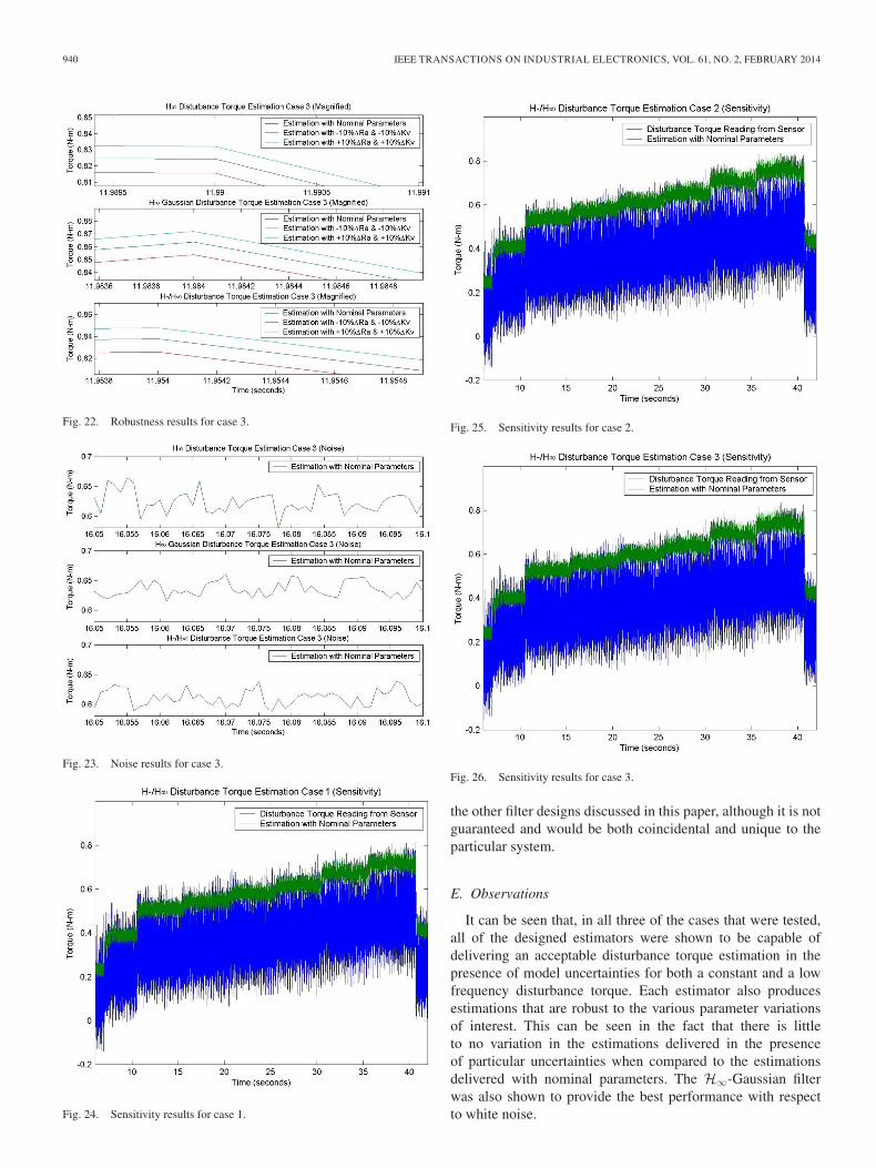
D. H−/H∞ Sensitivity Results

Since sensitivity to a disturbance is also a requirement in thedesign of the H−/H∞ filter-based disturbance torque estimator,a second set of tests was also conducted to ensure that thisrequirement was achieved by the design of the H−/H∞ filter-based estimators. It can be seen in Figs. 24–26 that smallchanges in the disturbance torque can be quickly reflected inthe disturbance torque estimation in all cases. This confirmsthat the H−/H∞ filter-based disturbance torque estimator notonly achieves robustness to model uncertainties but also simul-taneously can maximize sensitivity to the disturbance torque.Note that this level of sensitivity may also be achieved using




Fig. 24. Sensitivity results for case 1.



the other filter designs discussed in this paper, although it is notguaranteed and would be both coincidental and unique to theparticular system.

E. Observations

It can be seen that, in all three of the cases that were tested,all of the designed estimators were shown to be capable ofdelivering an acceptable disturbance torque estimation in thepresence of model uncertainties for both a constant and a lowfrequency disturbance torque. Each estimator also producesestimations that are robust to the various parameter variationsof interest. This can be seen in the fact that there is littleto no variation in the estimations delivered in the presenceof particular uncertainties when compared to the estimationsdelivered with nominal parameters. The H∞-Gaussian filterwas also shown to provide the best performance with respectto white noise.


It can also be seen that the H−/H∞ filter that was originallydesigned for use in fault detection can also be applied tothe design of a disturbance torque estimator, thus providingdesigners with another option for filter design when designingan estimator. This filter design not only is robust to uncertaintiesbut was also shown to have the added benefit of maximumsensitivity to a disturbance.

In summary, the H∞ filter is suitable for an application thatrequires the estimation to be robust to model uncertainties.The H∞-Gaussian filter is suitable for an application thatrequires the estimation to be robust to model uncertainties andto suppress white noise. The H−/H∞ filter is suitable for anapplication that requires the estimation to be robust to modeluncertainties and sensitive to the disturbance torque.

Further improvement of the estimation may be done by fine-tuning the parameters γ, w1, w2, and w3 as needed so as tovary the degree of tolerance of the observer or to vary thesignificance of the particular uncertainty on the disturbancetorque estimation.

V. CONCLUSION

In this paper, we have carried out designs for three distur-bance torque estimators that can be used to robustly estimatethe disturbance torque in a motor drive system in the presenceof parameter variations and/or noise. In particular, an H∞ filter,an H∞-Gaussian filter, and an H−/H∞ filter were used as thebasis for the designs from which the disturbance torque wasthen estimated.

The H−/H∞ filter is a new and novel approach to distur-bance torque estimator design since it was originally designedfor fault detection and has never previously been used in adisturbance torque estimation application. This filter designguarantees not only robustness to uncertainties but also max-imum sensitivity to a disturbance and can be of great benefit todesigners. Previous designs do not guarantee such performance.

It was shown that these designs can estimate not only aconstant disturbance torque but also one that varies at a lowfrequency. This is guaranteed with these designs, and again,previous designs do not guarantee this type of performance.

Hardware tests were conducted using a real PMDC that wassubjected to both a disturbance torque and parameter variations.The estimators were implemented using a real-time computer.Three cases of parameter variations were considered. In allcases, the estimators were tested using both a constant distur-bance torque and one that varied at a low frequency. The resultswere validated using an in-line torque sensor and confirmed thatthe estimators deliver a robust disturbance torque estimation inthe presence of parameter variations.

The following guidelines are proposed for the selection ofan appropriate filter design based on the requirements of thesystem. If robustness to uncertainties is the only concern inthe design of the estimator, then an H∞ filter-based design isrecommended. If both robustness to uncertainties and noise areconcerns, then an H∞-Gaussian filter-based design is recom-mended. If both robustness to uncertainties and sensitivity to adisturbance are concerns, then an H−/H∞ filter-based designis recommended.

TABLE IIPARAMETERS OF THE TEST MOTOR

TABLE IIIPARAMETERS USED TO DETERMINE THE OBSERVER GAINS

TABLE IVOBSERVER GAINS FOR THE H∞ FILTER

TABLE VOBSERVER GAINS FOR THE H∞-GAUSSIAN FILTER

TABLE VIOBSERVER GAINS FOR THE H−/H∞ FILTER

APPENDIX

The parameters of the PMDC used to test the designedestimators are listed in Table II. The parameters used to cal-culate the observer gains are listed in Table III. The calculatedobserver gains are listed in Tables IV–VI.


REFERENCES

[1] G. S. Buja, R. Menis, and M. I. Valla, “Disturbance torque estimation in asensorless dc drive,” IEEE Trans. Ind. Electron., vol. 42, no. 4, pp. 351–357, Aug. 1995.

[2] H. Chaal and M. Jovanovic, “Practical implementation of sensorlesstorque and reactive power power control of doubly fed machines,” IEEETrans. Ind. Electron., vol. 59, no. 6, pp. 2645–2653, Jun. 2012.

[3] X. Chen and K. Zhou, “Multiobjective H2/Hinf control design,” SIAM J.Control Optim., vol. 40, no. 2, pp. 628–660, 2001.

[4] X. Chen and K. Zhou, “H∞-Gaussian filter on infinite time horizon,”IEEE Trans. Circuits Syst. I, Fundam. Theory Appl., vol. 49, no. 5,pp. 674–679, May 2002.

[5] R. Errouissi, M. Ouhrouche, W. Chen, and A. M. Trzynadlowski,“Robust cascaded nonlinear predictive control of a permanent-magnetsynchronous motor with antiwindup compensator,” IEEE Trans. Ind.Electron., vol. 59, no. 8, pp. 3078–3088, Aug. 2012.

[6] J. Guzinski, H. Abu-Rub, M. Diguet, Z. Krzeminski, and A. Lewicki,“Speed and load torque observer application in high-speed train electricdrive,” IEEE Trans. Ind. Electron., vol. 57, no. 2, pp. 565–574, Feb. 2010.

[7] W. S. Huang, C. W. Liu, P. L. Hsu, and S. S. Yeh, “Precision con-trol and compensation of servomotors and machine tools via the distur-bance observer,” IEEE Trans. Ind. Electron., vol. 57, no. 1, pp. 420–429,Jan. 2010.

[8] S. H. Kia, H. Henao, and G. E. Capolino, “Torsional vibration assessmentusing induction machine electromagnetic torque estimation,” IEEE Trans.Ind. Electron., vol. 57, no. 1, pp. 209–219, Jan. 2010.

[9] M. Lawson and X. Chen, “Fault tolerant control for an electricpower steering system,” in Proc. IEEE Int. Conf. Control Appl., 2008,pp. 486–491.

[10] M. Lawson and X. Chen, “Hardware-in-the-loop simulation of fault tol-erant control for an electric power steering system,” in Proc. IEEE Veh.Power Propulsion Conf., 2008, pp. 1–6.

[11] X. Li and K. Zhou, “A time domain approach to robust fault detection oflinear time-varying systems,” in Proc. 46th IEEE Conf. Decision Control,2007, pp. 1015–1020.

[12] X. Li and K. Zhou, “A time domain approach to robust fault detectionof linear time-varying systems,” Automatica, vol. 45, no. 1, pp. 94–102,Jan. 2009.

[13] N. Liu and K. Zhou, “Optimal solutions to multi-objective robust faultdetection problems,” in Proc. 46th IEEE Conf. Decision Control, 2007,pp. 981–988.

[14] N. Liu and K. Zhou, “Optimal robust fault detection for linear discretetime systems,” J. Control Sci. Eng., vol. 2008, p. 7, Jan. 2008.

[15] D. G. Luenberger, “Observing the state of a linear system,” IEEE Trans.Mil. Electron., vol. MIL-8, no. 2, pp. 74–80, Apr. 1964.

[16] D. G. Luenberger, “An introduction to observers,” IEEE Trans. Autom.Control, vol. AC-16, no. 6, pp. 596–602, Dec. 1971.

[17] N. Mohan, T. M. Undeland, and W. P. Robbins, Power Electronics: Con-verters, Applications, and Design. Hoboken, NJ, USA: Wiley, 2003.

[18] K. Natori, T. Tsuji, K. Ohnishi, A. Hace, and K. Jezernik, “Time-delaycompensation by communication disturbance observer for bilateral tele-operation under time-varying delay,” IEEE Trans. Ind. Electron., vol. 57,no. 3, pp. 1050–1062, Mar. 2010.

[19] J. W. Park, S. H. Hwang, and J. M. Kim, “Sensorless control of brushlessdc motors with torque constant estimation for home appliances,” IEEETrans. Ind. Appl., vol. 48, no. 2, pp. 677–684, Mar./Apr. 2012.

[20] G. G. Rigatos, “A derivative-free Kalman filtering approach to stateestimation-based control of nonlinear systems,” IEEE Trans. Ind. Elec-tron., vol. 59, no. 10, pp. 3987–3997, Oct. 2012.

[21] J. Shawash and D. R. Selviah, “Real-time nonlinear parameter estimationusing the Levenberg-Marquardt algorithm on field programmable gatearrays,” IEEE Trans. Ind. Electron., vol. 60, no. 1, pp. 170–176, Jan. 2013.

[22] D. Simon, Optimal State Estimation: Kalman, H-Infinity, and NonlinearApproaches. Hoboken, NJ, USA: Wiley, 2006.

[23] Y. I. Son, H. Shim, N. H. Jo, and S. J. Kim, “Design of disturbanceobserver for non-minimum phase systems using PID controllers,” in Proc.SICE Annu. Conf., 2007, pp. 196–201.

[24] C. C. Wang and M. Tomizuka, “Design of robustly stable disturbanceobservers based on closed loop consideration using Hinf optimization andits applications to motion control systems,” in Proc. Amer. Control Conf.,2004, pp. 3764–3769.

[25] F. Zhang, G. Liu, L. Fang, and H. Wang, “Estimation of battery stateof charge with H∞ observer: Applied to a robot for inspecting powertransmission lines,” IEEE Trans. Autom. Control, vol. 59, no. 2, pp. 1086–1095, Feb. 2012.

[26] K. Zhou and J. C. Doyle, Essentials of Robust Control. Upper SaddleRiver, NJ, USA: Prentice-Hall, 1998.

[27] K. Zhou and Z. Ren, “A new controller architecture for high performance,robust, and fault-tolerant control,” IEEE Trans. Autom. Control, vol. 46,no. 10, pp. 1613–1618, Oct. 2001.

Danny Grignion (S’09–M’12) received the B.A.Sc.and M.A.Sc. degrees in electrical engineering fromthe University of Windsor, Windsor, ON, Canada, in2010 and 2012, respectively.

He is working in industry in the field of industrialautomation and control.

Xiang Chen (M’98) received the M.Sc. and Ph.D.degrees in systems and control from Louisiana StateUniversity, Baton Rouge, LA, USA, in 1996 and1998, respectively.

He was with Lakehead University, Thunder Bay,ON, Canada, from 1998 to 1999. Since 2000, he hasbeen with the Department of Electrical and Com-puter Engineering, University of Windsor, Windsor,ON, Canada, where he is currently a Professor. Hisresearch interests include robust control, control ofcomplex systems, networked control systems, and

industrial applications of control theory.

Narayan Kar (S’95–M’00–SM’07) received theB.Sc. degree in electrical engineering from theBangladesh University of Engineering and Technol-ogy, Dhaka, Bangladesh, in 1992 and the M.Sc.and Ph.D. degrees in electrical engineering from theKitami Institute of Technology, Hokkaido, Japan, in1997 and 2000, respectively.

He is an Associate Professor in the Department ofElectrical and Computer Engineering, University ofWindsor, Windsor, ON, Canada, where he holds theCanada Research Chair position in hybrid drivetrain

systems. His research presently focuses on the analysis, design, and control ofpermanent-magnet synchronous, induction, and switched reluctance machinesfor electric and hybrid electric vehicle and wind power applications, testing andperformance analysis of batteries, and development of optimization techniquesfor hybrid energy management systems.

Huijie Qian received the B.A.Sc. degree in electricalengineering from Shanghai Jiao Tong University,Shanghai, China, in 2010 and the M.A.Sc. degree inelectrical engineering from the University of Wind-sor, Windsor, ON, Canada, in 2012, focusing ondiscrete-time control systems.

He is currently with the Department of Electricaland Computer Engineering, University of Windsor.

estimation of load disturbance torque for dc motor drive systems under robustness and sensitivity...

Documents

robust estimation

load torque

disturbance torqueacting

nearlyconstant disturbance

estimation hasbecome

everyday systems

highlysensitive systems

motors shaft