estimation of oxide growth on joint surfaces during fsw ... · pdf filereport author matts...

Public Document ID 1402837

Version 1.0

Status Approved

Reg no (13)

Report Author Matts Björck

Date 2013-08-07

Reviewed byLisette Åkerman (QA)

Reviewed date2015-02-27

Approved byJan Sarnet

Approved date2015-02-27

Estimation of oxide growth on joint surfaces during FSW

Svensk Kärnbränslehantering ABSwedish Nuclear Fuel and Waste Management CoPO Box 925, SE-572 29 OskarshamnVisiting address Gröndalsgatan 15Phone +46-491-76 79 00 Fax +46-491-76 79 30www.skb.se556175-2014 Seat Stockholm

AbstractA previously developed model of the oxidation kinetics of pure copper in an Ar/O2 atmosphere is applied to the case of Friction Stir Welding of copper canisters. In order to apply the model the experimental temperature history of the joint surfaces together with metallographic is used as input. Ambient oxygen levels results in maximum oxygen content of about 100 wt-ppm in the weld material. If the oxygen concentration in the surrounding atmosphere during welding is lowered to 100mol-ppm�� the resulting increase in the oxygen concentration in the weld material will be below 1wt-ppm. At these and lower oxygen concentrations the native oxide film formed prior to welding is a significant contribution to the increase in the oxygen content in the weld material.

PDF

rend

erin

g: D

okum

entID

140

2837

, Ver

sion

1.0,

Sta

tus

God

känt

, Sek

rete

sskla

ss Ö

ppen

1402837 - Estimation of oxide growth on joint surfaces during FSW

Public 1.0 Approved 2 (13)

Svensk Kärnbränslehantering ABSwedish Nuclear Fuel and Waste Management Co

1 IntroductionAs friction stir welding (FSW) is a solid state joining process most produced welds contains elevated amounts of oxygen. This is caused by a combination of elevated temperatures and access to oxygen prior to the joining of the joint surfaces. The streaks of embedded oxide particles for the copper welds produced by SKB have not been shown to have a detrimental effect on the mechanical properties (Andersson-Östling and Sandström 2009) nor have they shown an effect in previous corrosion experiments (Gubner and Andersson 2007). However, the oxide streaks are considered an imperfection and should, consequently, be minimized.

One way to reduce the amount of oxides is to lower the oxygen content in the atmosphere around the joint line. This is usually done by protecting the joint surfaces with an inert gas, such as argon. The FSW machine at the canister laboratory has been fitted with a gas shield during the last years. When developing such a gas shield it is natural to consider which oxygen partial pressure should be kept within the shield.

In order to answer this question an experimental program has been set up at the canister laboratory. The first step consisted of a literature study combined with an experimental study (SKBdoc 1410172) to determine the oxidation kinetics of copper surfaces exposed to various oxygen partial pressures. This resulted in a model that can calculate the amount of oxide formed given the temperature, time and oxygen content available. The remaining part, which will be dealt with in this report, consists of using the temperature history at the joint line to estimate the amount of oxide formed during welding for different oxygen partial pressures.

2 Theory

2.1 Oxidation kineticsThe oxidation kinetics of copper was reviewed and completed with experimental measurements in“Oxidation kinetics of copper at reduced oxygen partial pressures” (SKBdoc 1410172). As the oxygen partial pressure is decreased there will be a transition from parabolic to linear kinetics. The parabolic rate constant has a limited dependence on the oxygen pressure whereas the linear rate constant has a linear dependence on the oxygen partial pressure. The rate equation can be written as

��+ ��

��= �, (2-1)

Where t is the time and x the weight per area unit of oxide formed. �� and �� are the parabolic and linear rate constants, respectively. This equation can be re-cast into a differential form which is applicable when �� and �� are time dependent, for example when the oxygen partial pressure or the temperature are changing. The differential form is consequently written as

��+ �� = ��. (2-2)

The differential equation can be integrated numerically as shown in the implementation in Appendix A. The constants �� and �� can be parameterized by using an Arrhenius expression for the temperature dependent part and a power law for the oxygen partial pressure, �� which becomes

��, �� = �� ,��

��,��

��,�� + ��,��

��,�� (2-3)

and

��, �� = �� ,��

��

��

��

��

�. (2-4)

The parameters in the above equations are given in Table 2-1. These parameters are the results of fitting the model parameters to thermogravimetric data in a range from 100mol-ppm�� to

PDF

rend

erin

g: D

okum

entID

140

2837

, Ver

sion

1.0,

Sta

tus

God

känt

, Sek

rete

sskla

ss Ö

ppen




21mol-%��. For further details the reader is referred to “Oxidation kinetics of copper at reduced oxygen partial pressures” (SKBdoc 1410172).

Table 2-1. The parameters used to describe the oxidation kinetics.

Parameter Value

�� 1.19 ∙ 10��/(��)

�� 27��/��

�� 1.04

��,� 21%

��,� 1000��

�� 1173.15°�

��,� 634��/(��)

��,� 248��/��

��,� 8.67 ∙ 10��/(��)

��,� 103��/��

�� 0.0

�� 0.83

2.2 Model of oxidation during FSW

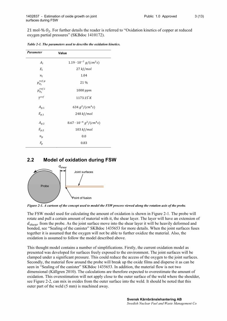
Figure 2-1. A cartoon of the concept used to model the FSW process viewed along the rotation axis of the probe.

The FSW model used for calculating the amount of oxidation is shown in Figure 2-1. The probe will rotate and pull a certain amount of material with it, the shear layer. The layer will have an extension of �� from the probe. As the joint surface move into the shear layer it will be heavily deformed and bonded, see “Sealing of the canister” SKBdoc 1435653 for more details. When the joint surfaces fuses together it is assumed that the oxygen will not be able to further oxidize the material. Also, the oxidation is assumed to follow the model described above.

This thought model contains a number of simplifications. Firstly, the current oxidation model as presented was developed for surfaces freely exposed to the environment. The joint surfaces will be clamped under a significant pressure. This could reduce the access of the oxygen to the joint surfaces. Secondly, the material flow around the probe will break up the oxide films and disperse it as can be seen in “Sealing of the canister” SKBdoc 1435653. In addition, the material flow is not two dimensional (Källgren 2010). The calculations are therefore expected to overestimate the amount of oxidation. This overestimation will not apply close to the outer surface of the weld where the shoulder, see Figure 2-2, can mix in oxides from the outer surface into the weld. It should be noted that this outer part of the weld (5 mm) is machined away.

PDF

rend

erin

g: D

okum

entID

140

2837

, Ver

sion

1.0,

Sta

tus

God

känt

, Sek

rete

sskla

ss Ö

ppen




Figure 2-2. A side view of the probe and shoulder relative to the outer surface of the weld.

2.3 Effect of surface oxides on total oxygen contentThe tube and lid material used in trial production is oxygen free phosphorus copper (Cu- OFP) which is specified to have an oxygen content less than 5wt-ppm(SKB 2010). Typical sample sizes for measuring the oxygen content by melt extraction are a cube with side � = 5mm. It is instructive to estimate the effect of oxidized joint surfaces on the measured oxygen content. Assuming that the oxidized surfaces will largely remain intact during the process, which is a pessimistic assumption given the stirring action of the FSW tool, the calculations simplifies to calculating the oxygen content in the aforementioned cube containing an oxide layer of thickness �. The molar density � of a component can be written as

� =��,

where � is the mass density, � is the molar mass and � is the volume. The volume of the oxide layer is �� = �� and the total volume of the sample is�� = ��. When copper oxidize two different copper oxides can form, either cupric oxide �� or cuprous oxide�� which has different oxygen molar densities, see Table 2-2. According to Zhu et al. (2006) �� dominates the oxide layer formedin air for temperatures above350℃. This is also the assumption used in SKBdoc 1410172 to transform the measured and modelled weight gains to thicknesses. Consequently, the same assumption will be used here to transform the modelled thicknesses to weight values as this will remove any systematic errors.

The base material has an oxygen concentration, ��,�� = ��,�� ⁄ . The concentration of oxygen in the sample is

�� =��,�� + ��,��

��≈

��

+ ��,�� = ��+ ��,��,

where it has been assumed that �� ≪ ��. The constant

� =��

��

.

Table 2-2. Material properties used in the calculation of the oxygen content.

Compound Molar mass, �[�/��]

Density, �[�/��]

�� [��/��

�] �

�� 79.545 6.315 0.0794 0.142

�� 143.09 6.0 0.0419 0.0748

�� 63.546 8.96 0.141 -

� 15.9994 - - -

The oxygen content in the sample as a function of the oxide thickness as given by the expression above can be seen in Figure 2-3. In order for the increase in oxygen content in the sample to be on the

PDF

rend

erin

g: D

okum

entID

140

2837

, Ver

sion

1.0,

Sta

tus

God

känt

, Sek

rete

sskla

ss Ö

ppen




same order of magnitude as the base material (< 5wt-ppm) the oxide layer thickness has to be about 0.1��.

Figure 2-3. The increase in oxygen content as a function of oxide thickness on a micro meter scale (left) and on a nano meter scale (right). As a comparison the base material Cu-OFP has oxygen content of below�� as indicated by the blue dotted line.

3 Experimental detailsThe temperature measurement during welding were conducted by placing type K thermocouples close to the joint line by drilling holes into the ring and lid to be welded. A total of 18 thermocouples were placed around the weld to monitor the temperature at several points. Three of the thermocouples were placed to create a depth profile 2 mm from the joint line. The temperatures were sampled at 8 Hz with a Eurotherm 6100 A data logger. A more detailed description of the experimental setup can be found in “Oxidation kinetics of copper at reduced oxygen partial pressures” (SKBdoc 1410172).

The metallographic examinations were taken from sectioning exit holes from weld FSW99. The samples were metallographically prepared and studied with a stereomicroscope macroscopically as well as with a microscope to reveal the details of remaining joint. The results are presented in “Metallographic examination of exit holes in FSWL99” (SKBdoc 1407047).

4 Results and Discussion

4.1 Metallographic investigationAn example of a prepared sample is shown in Figure 4-1. The distance between the rim of the hole to the non-bonded joint is �� = 2.5��. This distance will decrease to �� = 1.6�� at the tip of the tool and further increase to �� = 2.8�� about 1.5�� from the surface of the canister.

PDF

rend

erin

g: D

okum

entID

140

2837

, Ver

sion

1.0,

Sta

tus

God

känt

, Sek

rete

sskla

ss Ö

ppen




Figure 4-1. Two macrographs(id: FSW99 113 deg T2 and FSW99 113 deg T3 ) an exit hole. The bright yellow horizontal line to the right is the unbonded remaining joint line. The right section is taken closer to the root of the weld whereas the left is taken closer to the surface. The more fine grained area is the welded material. The semicirculair features seen on the left picture are optical artefacts from the microscope. See SKBdoc 1407047 for further details.

4.2 Temperature profileDuring the measurements the probe broke before arriving to the final three thermocouples that were placed at the joint line. Therefore only one thermocouple, the one closest to the surface, gives a, for the process, valid reading. The temperature evolution for that thermocouple is shown in Figure 4-2. The first maxima arise due to the heating during the start sequence; the thermocouples are located directly below the plunge position. After welding around the canister the probe arrives to the thermocouple position again to complete the joint. This creates the leftmost and highest peaks in the graph.

Using the speed of the machine and the peaks in the thermocouples located at the depth from the surface at a distance of 180° away from the outermost thermocouple it is possible to estimate where the centre of the tool crosses the thermocouple position (calculated to occur at time 14:11:45). Then using the thickness of the shear layer measured in section 4.1 combined with the measured diameter of the exit hole (5.1 − 13��) an interval where the joint was created can be estimated. These distances can be recalculated to time by using the welding speed, 80��/��. The resulting points are shown in Figure 4-3. As the thermocouple is placed closer to the surface it can be expected that the maximum temperature reached is about 800℃. If the position of the joining at the root is used instead the maximum temperature would be 900℃ that would be constant for5� assuming that the temperature profile would be constant. However, the thermocouple is located at the outer surface and consequently the temperature used in the following calculations will assume that the surfaces join just before the first drop in the temperature readings.

PDF

rend

erin

g: D

okum

entID

140

2837

, Ver

sion

1.0,

Sta

tus

God

känt

, Sek

rete

sskla

ss Ö

ppen




Figure 4-2. Three thermocouples recordings for the thermocouples located closest to the joint line. �� denote the distance from the outer surface of the weld.

Figure 4-3. The temperature as a function of time for the thermocouple located closest to surface, red line, with vertical lines showing the different events that are discussed in the text.

The temperature recorded under the starting position will probably not be the one that cause the most oxidation. Instead the position that will have the highest temperature for the longest time will be the joint surfaces next to the beginning of the joint line sequence as shown in Figure 4-4. As no measurements were made at this position the temperatures will be estimated instead. The highest measured temperature in weld FSWL94 (SKBdoc 1371191) that was not part of the weld zone was the thermocouple located at 181.5° with a maximum temperature of713℃. Consequently this data set has been used to replace the beginning of the data set in Figure 4-2 for�� = 5��. This will be used as one of two cases analysed further in the next section.

PDF

rend

erin

g: D

okum

entID

140

2837

, Ver

sion

1.0,

Sta

tus

God

känt

, Sek

rete

sskla

ss Ö

ppen




Figure 4-4. A picture denoting the different sequences during welding: The dwell and start sequence (1), the downward sequence(2), the joint line sequence (3), the overlap sequence (4) and the parking sequence (5).

4.3 Oxidation evolutionUsing the temperature curves discussed above as input in the oxidation kinetics model the evolution of the oxide thickness as a function of time for different scenarios can be calculated. Glow Discharge –Optical Emission depth profiling (SKBdoc 1407846) has shown that using the joint preparation procedure currently used1 before welding the oxide thickness is below10��. However, other labs have reported that clean copper surfaces have an oxide thickness of about1��, see references in “Oxidation kinetics of copper at reduced oxygen partial pressures” (SKBdoc 1410172). Therefore both of these scenarios will be used in the subsequent calculations. Two different temperature evolutions will be used. One of them is representing an estimation of the beginning of the joint line sequence and the other a measured curve below the starting hole.

4.3.1 Atmospheric conditions

The resulting oxidation growth curve for atmospheric conditions, 21mol-%��, is shown in Figure 4-5. As can be seen in the figure the oxide thickness reaches a thickness of4��for the temperature evolution corresponding to the beginning of the joint line sequence. In “Oxidation kinetics of copper at reduced oxygen partial pressures” (SKBdoc 1410172) some spallation was observed during the experiments. This can occur upon rapid temperature changes and thick films. This can be modelled as a restart of the oxidation after a sharp temperature drop. Doing this calculation (not shown here) yield a maximum oxide thickness of 5�� for the temperature evolution at the beginning of the joint line sequence. Consequently, the effect of spallation is estimated to be 20 % in this case.

1 The preparations are dry milling of joint surfaces, abrasive cleaning and spraying with ethanol and subsequent wiping using lint free paper.

PDF

rend

erin

g: D

okum

entID

140

2837

, Ver

sion

1.0,

Sta

tus

God

känt

, Sek

rete

sskla

ss Ö

ppen




Figure 4-5. The oxide thickness (top) as a function of time for��mol-%�� and temperature according to the lower panel. Full lines correspond to a position under the starting hole and dashed line to the beginning of the joint line sequence.

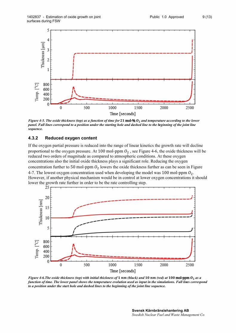
4.3.2 Reduced oxygen contentIf the oxygen partial pressure is reduced into the range of linear kinetics the growth rate will decline proportional to the oxygen pressure. At 100mol-ppm�� , see Figure 4-6, the oxide thickness will be reduced two orders of magnitude as compared to atmospheric conditions. At these oxygenconcentrations also the initial oxide thickness plays a significant role. Reducing the oxygen concentration further to 50mol-ppm�� lowers the oxide thickness further as can be seen in Figure 4-7. The lowest oxygen concentration used when developing the model was 100mol-ppm��. However, if another physical mechanism would be in control at lower oxygen concentrations it shouldlower the growth rate further in order to be the rate controlling step.

Figure 4-6.The oxide thickness (top) with initial thickness of �� (black) and �� (red) at ��mol-ppm�� as a function of time. The lower panel shows the temperature evolution used as input in the simulations. Full lines correspond to a position under the start hole and dashed lines to the beginning of the joint line sequence.

PDF

rend

erin

g: D

okum

entID

140

2837

, Ver

sion

1.0,

Sta

tus

God

känt

, Sek

rete

sskla

ss Ö

ppen




Figure 4-7. Same information as in Figure 4-6 for ��mol-ppm��.

4.4 Effects on the oxygen levels in the weldAt atmospheric conditions the oxygen layer thickness on one surface is calculated to be 4��, thus the total oxide thickness would be 8�� for two surfaces. According to Figure 2-3 this translates to an oxygen content of 100wt-ppm in a sample. This is higher than the maximum value seen in FSW27 (SKBdoc 1238519), 44 ± 12wt-ppm, that was produced in air. That can be expected as the probe disperses the oxide layer in the weld zone and thus lower the oxygen content compared to the simplified model.

If oxygen concentration in the environment is reduced to 100mol-ppm the maximum oxide thickness will be 20 − 50�� which translate to an increase in oxygen content of 0.3 − 0.8wt-ppm. Reducing the oxygen concentration further to 50mol-ppm causes the increase in oxygen concentration in the sample to be < 0.5wt-ppm.

5 ConclusionsGiven that the oxide layer on the joint surfaces are below 10�� and that the oxygen concentration at the weld surfaces are below 100mol-ppm the calculations presented here indicate that the increase in oxygen content in the weld zone will be below 1wt-ppm. An oxygen concentration of 100mol-ppmwill keep the oxide film at the same order of magnitude as for an initial oxide thickness of 10��. An oxygen partial pressure of 50mol-ppm and an initial oxide thickness of 1�� will keep the oxide thickness formed below 10 nm.

6 ReferencesAndersson-Östling H C M, Sandström R, 2009. Survey of creep properties of copper intended for nuclear waste disposal. SKB TR-09-32, Svensk Kärnbränslehantering AB.

Gubner R, Andersson U, 2007. Corrosion resistance of copper canister weld material. SKB TR-07-07, Svensk Kärnbränslehantering AB.

Källgren T, 2010. Investigation and modelling of friction stir welded copper canisters. PhD thesis. Royal Institute of Technology, Sweden.

PDF

rend

erin

g: D

okum

entID

140

2837

, Ver

sion

1.0,

Sta

tus

God

känt

, Sek

rete

sskla

ss Ö

ppen




SKB, 2010. Design, production and initial state of the canister. SKB TR-10-14, Svensk Kärnbränslehantering AB.

Zhu Y, Mimura K, Lim J-W, Isshiki M, Jiang Q, 2006. Brief review of oxidation kinetics of copper at 350 °C to 1050 °C. Metallurgical and Materials Transactions A 37, 1231–1237.

Unpublished documents

SKBdoc id, version Title Publisher, year

1238519 ver 1.0 Technical report of SKB FSW chemical analysis Luvata Pori Oy, 2010

1371191 ver 1.0 FSWL94 – Measurement of temperatures and surrounding oxygen levels during welding

SKB, 2013

1407047 ver. 1.0 Metallographic examination of exit holes in FSWL99 SKB, 2013

1407846 ver 1.0 Undersökning av rengöringsmetoder och oxidation av kopparytor i ädelgas med GD-OES. (In Swedish.)

SKB, 2013

1410172 ver 1.0 Oxidation kinetics of copper at reduced oxygen partial pressures

SKB, 2013

1435653 ver 1.0 Sealing of the canister SKB, 2014

1238519, ver 1.0 Technical report of SKB FSW chemical analysis rev2, Luvata

Luvata Pori Oy, 2010

PDF

rend

erin

g: D

okum

entID

140

2837

, Ver

sion

1.0,

Sta

tus

God

känt

, Sek

rete

sskla

ss Ö

ppen




7 Appendix AThe program code, written in Python, used for the simulations is given below.# -*- coding: utf-8 -*-"""A script to estimate the growth of Cu2O at different conditions.Programmer: Matts Bjorck, [email protected] modified: 2015-01-12"""

from numpy import *

# Constants usedpc, ppm = 1e-2, 1e-6h, min, s = 3600., 60., 1.

_plot = True

# Settings for the calculationsout_file = "O50ppm_d010nm"# Initial oxide thicknessd0 = 0.010 #mum# Set the oxygen partial pressure used in the calculationsoxygen_cont = 50*ppm

def x_to_d(x): """Transforms the weight gain , x, in g/cm2 to thickness, d, in mum""" return x*1.46e4

def d_to_x(AA): """Transforms the thickness, d, in mum to weight gain ,x, in g/cm2""" return AA/1.46e4

def calc_weight(time, temp, p_oxygen, x0): """Calculates the weight given the parameters with combination of linear and parabolic rate constantas according to Ronnqvist and Fischmeister. """ # Previously fitted constants A_p1 = 634 #g2/cm4/s A_p2 = 8.67e-4 #g2/cm4/s E_p1 = 248e3 #J/mol E_p2 = 103e3 #J/mol A_l = 1.19e-7 #g/cm2/s E_l = 27e3 #J/mol n_l = 1.04 n_p = 0.0 F_p = 0.83 p_refp = 0.21 p_refl = 1000e-6 # Transforming deg C to deg K T = temp + 273.15 # Defing constants # R - the gas cosntant R = 8.314 #J/mol/K kp = F_p*(p_oxygen/p_refp)**n_p*(A_p1*exp(-E_p1/R/T) + A_p2*exp(-E_p2/R/T)) kl = (p_oxygen/p_refl)**n_l*A_l*exp(-E_l/R*(1./T - 1./1173.15)) # Setting the first element to the pre-oxidezed value x = [x0] #Doing a forward integration for each time step for i in range(1,len(time)): dt = time[i] - time [i-1] av_kl = (kl[i] + kl[i-1])/2. av_kp = (kp[i] + kp[i-1])/2. dx = dt/(1.0/av_kl + 2*x[-1]/av_kp) x.append(x[-1] + dx) #return 0.5*(-kp/kl + sqrt((kp/kl)**2 + 4*kp*(time))) return array(x)

# Load temperatures for the position under the start pos.A = loadtxt('Data_for_oxidationslast.txt', delimiter = None, skiprows = 2)print A.shapetemp_start = A[:,1]time_start = A[:,0]-A[6000,0]

PDF

rend

erin

g: D

okum

entID

140

2837

, Ver

sion

1.0,

Sta

tus

God

känt

, Sek

rete

sskla

ss Ö

ppen




def create_worst_tempcase(): '''Assembles data for a worst case when the probe reach the joint line''' A1 = loadtxt('Data_for_oxidationslast.txt', delimiter = None, skiprows = 2) A2 = loadtxt('TempData_1815deg.txt', delimiter = None, skiprows = 2) offset1 = (-0/0.15607 + 750)/0.125 offset2 = (1153 - 60/0.15607 + 1140)/0.125 # Slice out the relevant parts maxind = min(A1.shape[0]-offset1, A2.shape[0]-offset2) cross = argmin(abs(A1[offset1:offset1 + maxind,1]-A2[offset2:offset2 + maxind,1])) merged = r_[A2[offset2:offset2+cross,1], A1[offset1 + cross:,1]] time = arange(len(merged))*0.125 return time, merged

# Load the data corresponding to the "worst case"time_worst, temp_worst = create_worst_tempcase()

# Tranform the initial oxide thickness to weightx0 = d_to_x(d0)# Calculate the "worst" cased_worst = x_to_d(calc_weight(time_worst, temp_worst, oxygen_cont, x0))# Calculate the thickness under the start holed_start = x_to_d(calc_weight(time_start, temp_start, oxygen_cont, x0))

# saving the results to filef = open(out_file + '_worst.dat','w')f.write('Time [s]\t Temperature [deg C]\t Oxygen content\t Oxide thickness [mum]\n')savetxt(f, c_[time_worst, temp_worst, oxygen_cont*(time_worst*0 + 1), d_worst])f.close()f = open(out_file + '_start.dat','w')f.write('Time [s]\t Temperature [deg C]\t Oxygen content\t Oxide thickness [mum]\n')savetxt(f, c_[time_start, temp_start, oxygen_cont*(time_start*0 + 1), d_start])f.close()

# Optional plottingif _plot: from pylab import * subplot(211) plot(time_worst[:]/60, d_worst) plot(time_start[:]/60, d_start) ylabel('Thickness [mum]') subplot(212) plot(time_worst/60., temp_worst) plot(time_start/60., temp_start) ylabel('Temperature [deg C]') show()

PDF

rend

erin

g: D

okum

entID

140

2837

, Ver

sion

1.0,

Sta

tus

God

känt

, Sek

rete

sskla

ss Ö

ppen

estimation of oxide growth on joint surfaces during fsw ... · pdf filereport author matts...

Documents