Estimation of saturation and pressure changes from time-lapse seismic data and model re-

parameterization for seismic history matching.

Dario GranaDepartment of Geology and Geophysics University of Wyoming

IOR workshop, 28 April 2016

Seismic reservoir characterization

– 2

• Seismic data S depend on reservoir properties R through elastic properties m

• We can split the inverse problem into two sub-problems:

•

• ff

gg

)(

)(

mR

Sm

))(( SR gf

seismic linearized modeling

rock physics model

Forward model

– 3

Seismic forward model:Wavelet convolution

Linearized Aki-Richards approximation of Zoeppritz equations

Wavelet Reflection coefficients Seismogram

),()( mhrPP

– 4

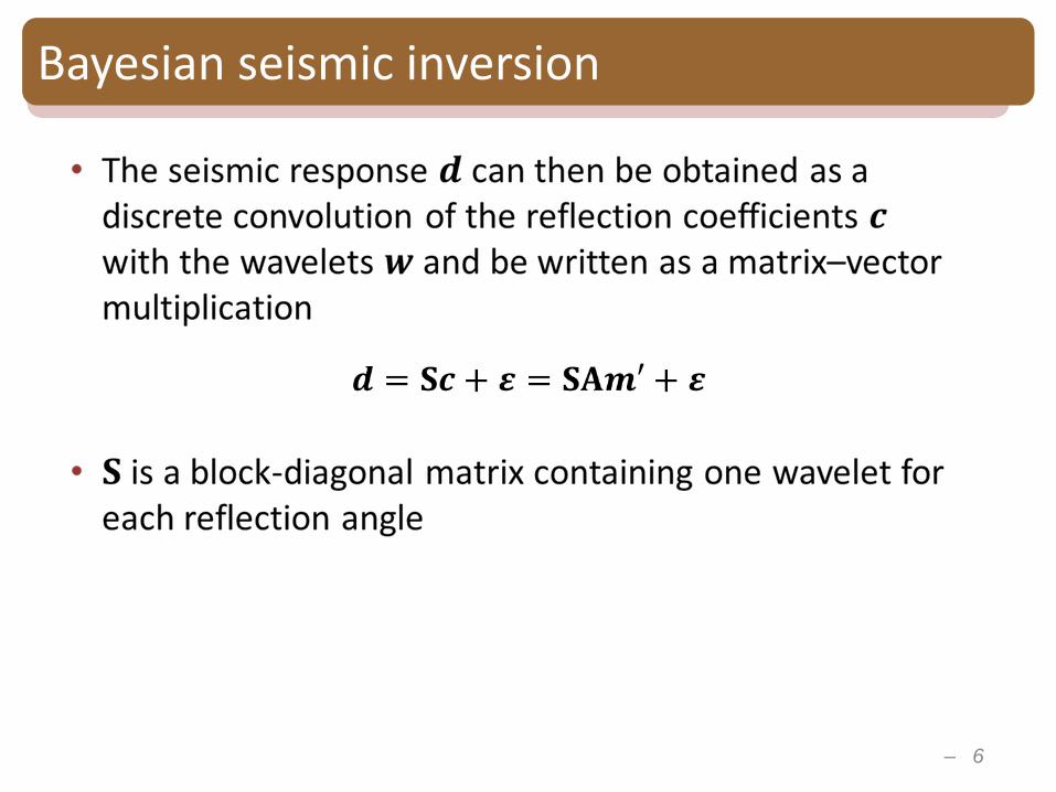
Bayesian seismic inversion

• The seismic response of a sequence of layers can be then written as:

• At a given time t, the reflections coefficients can be approximated by the three term Shuey approximation

– 5

Bayesian seismic inversion

– 6

Bayesian seismic inversion

– 7

Bayesian seismic inversion

Forward model

– 8

Rock physics forward model:

Granular media models (Hertz-Mindlin contact theory)

P-wave velocity versus effective porosity

sw

cfV

V

RPMS

P

Bayesian petrophysical inversion

Elastic properties

Seismic data)( Sm|P

Gaussian mixture

likelihood

)|( mRP

Rock properties

)( SR|P

(Chapman-Kolmogorov)

Grana and Della Rossa, 2010

Buland and Omre, 2003

– 10

Time-lapse inversion

• In time-lapse reservoir modeling we aim to model reservoir property changes from repeated seismic surveys.

Inverse problem

Time-lapse seismic dataReservoir property changes

(saturation and pressure)

Grana and Mukerji, 2014

Challenges

• Elastic changes introduce time-shifts in the repeated seismic surveys (either we invert amplitudes and travel time or we correct for time-shifts and invert for amplitudes)

• The link between dynamic properties and elastic properties is not direct. Need a RPM to transform pressure and saturation into elastic properties.

• Mapping of data between different grid representations corresponding to the flow simulation, earth model and seismic grid frameworks.

– 11

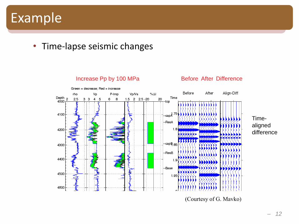
Example

• Time-lapse seismic changes

– 12

Increase Pp by 100 MPa Before After Difference

Time-

aligned

difference

(Courtesy of G. Mavko)

Methods

• Method 1: to simultaneously invert base and repeated seismic surveys

– 13

(Courtesy of P. Doyen)

Methods

• Method 2: to invert seismic changes (difference in amplitudes)

* We cannot compute the difference directly because horizons of the repeated surveys are not aligned with the base survey. We must apply a warping method first.

– 14

Methods

• 2-step approach

– 15

1. We first estimate

2. We then estimate

3. We combine and using Chapman-Kolmogorov equation

( | ) ( | ) ( )P P P m S S m m

( | ) ( | ) ( )P P P R m m R R

Buland and El Ouair, 2006

( | )P m S ( | )P R m

( | ) ( | ) ( | )m

P P P d

R S R m m S mGrana and Mukerji, 2014

Seismic model

– 16

Seismic forward model:Wavelet convolution

Linearized Aki-Richards approximation of Zoeppritz equations

Wavelet Reflection coefficients Seismogram

),()( mhrPP

MacBeth equation

( )

1 K

dry P

P

K

KK P

A e

Methods for seismic history matching

• Option1: to match production data and time-lapse seismic data

• Option 2: to match production data and inverted seismic velocities (or impedances)

• Option 3: to match production data and inverted pressure and saturation (or a re-parameterization)

(plus several options for the parameterization and for the inverse method)

– 18

– 19

Re-parameterized seismic history matching

Bayesian time-lapse inversion Re-parameterization

Seismic history matching

(ES-MDA)

Synthetic example: waterflooding

– 20

Synthetic reservoir model (modified from Panzeri et al., 2014)

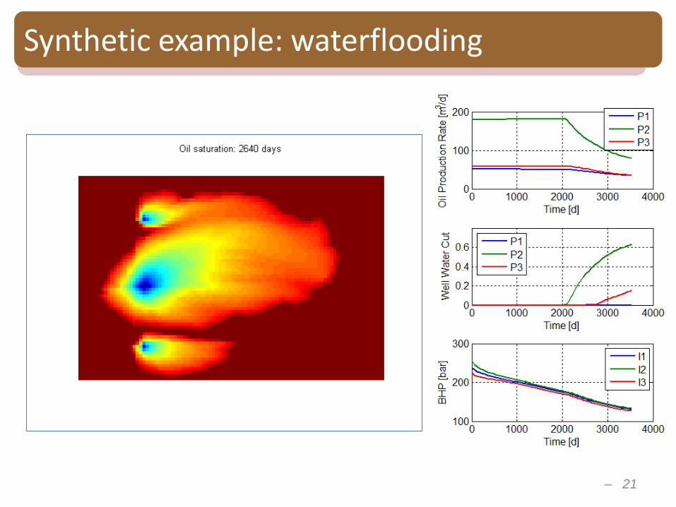
Synthetic example: waterflooding

– 21

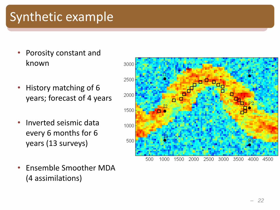
Synthetic example

– 22

• Porosity constant and known

• History matching of 6 years; forecast of 4 years

• Inverted seismic data every 6 months for 6 years (13 surveys)

• Ensemble Smoother MDA (4 assimilations)

Synthetic example

– 23

Synthetic example

– 24

Synthetic example

– 25

Synthetic example

– 26

Prior model

Updated model

Synthetic example: comparison

– 27

– 28

Acknowledgements

Thanks for your attention

• Thanks to Geir for the invitation

– 29

Methodology

• Bayesian time-lapse inversion for pressure and saturation changes

• Re-parameterization of saturation snapshots through POD-DEIM

• History matching of production data and re-parameterized inverted seismic data through ES-MDA

– 30

Re-parameterization

• If we match the seismic data pointwise, we need a large ensemble to avoid ensemble collapse

• We want to avoid to compute CDD

• Issues with resolution, noise, quality of seismic data

– 31

Proper Orthogonal Decomposition

– 32

Discrete Empirical Interpolation Method

– 33

Discrete Empirical Interpolation Method

Chaturantabut and Sorensen, 2010

• The projection basis is given by POD

• The interpolation indices are given by DEIM

– 34

Example 1

– 35

Example 1

Other parameterization methods: wavelet, DCT, waterfront, spatial PCA, ...