estimation of supply and demand elasticities of california
TRANSCRIPT

UC DavisAgriculture and Resource Economics Working Papers
TitleEstimation of Supply and Demand Elasticities of California Commodities
Permalinkhttps://escholarship.org/uc/item/3432z1pv
AuthorsRusso, CarloGreen, Richard D.Howitt, Richard E
Publication Date2008-06-01
eScholarship.org Powered by the California Digital LibraryUniversity of California

Department of Agricultural and Resource EconomicsUniversity of California, Davis
Estimation of Supply and Demand Elasticities of California Commodities
by
Carlo Russo, Richard Green, and Richard Howitt
Working Paper No. 08-001
June 2008
Copyright @ 2008 by Carlo Russo, Richard Green, and Richard Howitt
All Rights Reserved. Readers may make verbatim copies of this document for non-commercial
purposes by any means, provided that this copyright notice appears on all such copies.
Giannini Foundation of Agricultural Economics

ESTIMATION OF SUPPLY AND DEMAND ELASTICITIES OF CALIFORNIA COMMODITIES
by
Carlo Russo, Richard Green, and Richard Howitt
ABSTRACT
The primary purpose of this paper is to provide updated estimates of domestic own-price, cross-price and income elasticities of demand and estimated price elasticities of supply for various California commodities. Flexible functional forms including the Box-Cox specification and the nonlinear almost ideal demand system are estimated and bootstrap standard errors obtained. Partial adjustment models are used to model the supply side. These models provide good approximations in which to obtain elasticity estimates. The six commodities selected represent some of the highest valued crops in California. The commodities are: almonds, walnuts, alfalfa, cotton, rice, and tomatoes (fresh and processed). All of the estimated own-price demand elasticities are inelastic and, in general, the income elasticities are all less than one. On the supply side, all the short-run price elasticities are inelastic. The long-run price elasticities are all greater than their short-run counterparts. The long-run price supply elasticities for cotton, almonds, and alfalfa are elastic, i.e., greater than one. Policy makers can use these estimates to measure the changes in welfare of consumers and producers with respect to changes in policies and economic variables. Keywords: Consumer Economics: Empirical Analysis (D120); Agricultural Markets and Marketing (Q130); Agriculture: Aggregate Supply and Demand Analysis; Prices (Q110) This research project was funded by the California Department of Food and Agriculture. The authors very much appreciate helpful comments on earlier revisions by Steven Shaffer and Charles Goodman. Carlo Russo is a Ph.D. student in the Department of Agricultural Economics at University of California, Davis. He can be contacted by e-mail at [email protected]. Richard Green is a professor and Richard Howitt is a professor and department chair, both in agricultural and resource economics at UC Davis. They can be contacted by e-mail at [email protected] and [email protected], respectively.

ESTIMATION OF SUPPLY AND DEMAND ELASTICITIES OF CALIFORNIA COMMODITIES
by
Carlo Russo, Richard Green, and Richard Howitt
June 2008
Introduction1 California’s agricultural sector can be characterized as being in a constant state of
flux. On the consumer side of the market there have many changes in recent decades.
Demographically, the proportion of married women in the labor force over the past four
decades has doubled. In addition, demand patterns have been influenced by health and
diet concerns. For example, there has been a 350% increase in sales of organic foods
during the past decade. Demands for specialized and niche products are also on the
increase.
The structure of fresh vegetable sales are more concentrated with fewer and larger
retail buyers, and environmental regulations are being imposed to ensure better food
safety. Competition from foreign suppliers is increasing. Technological changes have
occurred in the processing of agricultural materials. Morrison-Paul and MacDonald
noted that food prices today often appear less responsive to farm price shocks than in the
past. Their research, however, found improving quality and falling relative prices for
agricultural inputs, in combination with increasing factor substitution, has counteracted
these forces to encourage greater usage of agricultural inputs in food processing.
________________________
1For an excellent discussion of the changes in California’s agricultural sector, see Johnson and McCalla.

On the production side, global markets and trade liberalization has greatly
impacted domestic markets. Land lost to urban expansion and an ever-growing pressure
on water available impact California producers. The number of farms in California is
decreasing while the sizes of farms are getting larger. While the price for California’s
fruits, nuts and vegetables is determined in domestic and export markets, the profitability
of competing field, fiber and fodder crops is influenced by federal subsidies and state
regulations. These impacts on California agriculture occur as both demand and supply
side policies change.
In order to better understand and evaluate the consequences of these changes on
consumer and producer welfare, it is essential to obtain reliable estimates of supply and
demand elasticities of California commodities. To the best of our knowledge, there is no
current comprehensive study that provides accurate up-to-date supply and demand
elasticity estimates of California’s major crops. Frequently cited works reporting demand
elasticities are Carole Nuckton’s Giannini Foundation publications (1978, 1980),
“Demand Relationships for California Tree Fruits, Grapes, and Nuts: A Review of Past
Studies” and “Demand Relationships for Vegetables: A Review of Past Studies”.
However, given the significant structural changes noted above, there are many causal
factors that need to be updated to generate current supply and demand elasticities.
A more recent article, “Demand for California Agricultural Commodities” by
Richard Green in the winter 1999 issue of Update reports estimates of own-price
elasticities for selected commodities. The commodities included food (in general),
almonds, California iceberg lettuce, California table grapes, California prunes, dried
fruits (figs, raisins, prunes), California avocados, California fresh lemons, California
2

residential water, and meats (beef, pork, poultry, and fish). All of the elasticity estimates
are reported in research publications by faculty of the Department of Agricultural and
Resource Economics at the University of California at Davis. Individual sources for the
commodities are given in the reference section.
The primary purpose of this research project is to obtain updated supply and
demand elasticity estimates of major California commodities. That is, short and long-run
own-price elasticities of supply and own price, cross-price and income elasticities of
demand. In this study sophisticatedly simple models are used (Zellner). The models
focus on California agriculture. As a consequence, we tried to emphasize the specificity
of California supply, contrasting it when possible, with aggregate US or the most relevant
competing states’ supply. Modeling the demand for California commodities was a
challenging task, considering that markets are integrated and often statistics about retail
prices do not discriminate products by origin. Also, for most crops we focused on the
demand at the wholesale level. Thus, farm gate price may be based on a standard “mark
down” of the price paid by the buyers. The modeling of wholesale demand was also
convenient for those products (for example nuts) that are consumed mostly as ingredients
of final goods. Exceptions to this approach relate to alfalfa and tomatoes. The former
commodity is a major input for the California dairy industry so we estimated a derived
demand. For fresh tomatoes we estimated the consumer demand at the US level.
Each crop presented specific modeling issues which are described in detail in
the following sections. A brief discussion of the theoretical foundations of the models
will be given, but detailed theoretical underpinnings of the models can be found in
standard microeconomic textbooks.
3
The analysis will start with some of the most highly valued crops in California:
almonds and walnuts, alfalfa hay, cotton, rice, and fresh and processing tomatoes. Future
research will examine grapes (including raisin, table, and wine); lettuce (head and leaf);
citrus (grapefruit, lemons, and oranges), stone fruits (apricots, nectarines, preaches,
plums, and prunes); and broccoli.
Before a discussion of the theoretical models, data sources, econometric
techniques, and the empirical results a brief literature review is provided.
Literature Review
1. Some Estimated Demand and Supply Elasticites from Previous Studies
One of the first attempts to compile a table of demand elasticity estimates for
California crops was Nuckton (1978). She reported own-price elasticity of demand
estimates for several California commodities including apples, cherries, apricots, peaches
and nectarines, pears, plums and prunes, grapes, grapefruit, lemons, oranges, almonds,
walnuts, avocados, and olives. Table 1 is a compilation of the empirical estimates that
Nuckton reported. Estimates for the different studies varied widely, but Table 1 attempts
to summarize the results from the main studies.
In 1999 Green published more recent elasticity estimates of California
commodities from various sources. The table of elasticity estimates is repeated below in
Table 2.
4

_______________________________________________________________________
Table 1. Selected Elasticity Estimates of California Commodities 1
Commodity Own-Price Elasticity Comments
of Demand _______________________________________________________________________
Apples -0.458 to –0.81 Fresh; some estimates were elastic
Cherries -4.27 Sweet; retail; based on 20 cities
Apricots -1.345 Fresh, farm level
Peaches & Nectarines -0.898 Fresh
Pears elastic Based on reciprocal price flexibilities
Plums and Prunes -0.630 Fresh, farm level
Grapes -0.327 (-0.267) –0.160 Fresh; table grapes (raisin) wine
Grapefruit -1.25 Fresh, retail level
Lemons -0.210 (-0.38) Fresh (processing)
Oranges -0.72 (-2.76) Fresh farm (fresh retail)
Almonds -1.74 (-14.164) Domestic shelled (export shelled)
Walnuts -0.464 Shelled; wholesale
Avocados elastic Based on reciprocal price flexibilities
Olives elastic Based on reciprocal price flexibilities
Source: Nuckton, C., “Demand Relationship for California Tree Fruits, Grapes, and
Nuts: A Review of Past Studies.” Giannini Foundation, August 1978.
5
Table 2. Estimates of Own-Price Elasticities for Selected Commodities 1
Commodity Own-Price Elasticity
Food (in general) -0.42
Almonds -0.83
California Iceberg Lettuce -0.16
California Table Grapes -0.28
California Prunes -0.44
Dried Fruits (Second Stage or Conditional)
Figs -0.23 Raisins -0.67
Prunes -0.35 California Avocados -0.86
California Fresh Lemons -0.34
Meats( Second Stage or Conditional)
Beef -0.84 Pork -0.79 Poultry -0.58 Fish -0.57 California Residential Water -0.16
Source: Green, R., “Demand for California Agricultural Commodities”, Update,
Department of Agricultural and Resource Economics, Vol. 2, No. 2, Winter, 1999.
_______________________________________________________________________
6

Some sources for the entries in Table 2 are as follows: food (Blanciforti, Green,
and King); California iceberg lettuce (Sexton and Zhang); dried fruits (Green, Carman,
and McManus); California avocados (Carman and Green); California fresh lemons
(Kinney, Carman, Green, and O’Connell); and California residential water (Renwick and
Green).
2. Examples of Market Conditions for Selected Commodities
A brief review of some recent selected articles illustrates the complexities of the
market conditions facing California producers and consumers. In addition, a discussion
of some economic factors that influence the supply and demand for certain products is
given. The market situation for different crops varies dramatically. For some
commodities, export and import markets are important. Other crops are perennial and
have to be model differently than annual crops. Expectations of producers have to be
incorporated in the supply response functions for these crops and a dynamic rather than a
static approach has to be used. Rotation patterns can affect the supply response for
certain crops such as alfalfa and cotton. A model for each crop has to incorporate these
unique market characteristics associated with that particular crop. A few examples of the
characteristic of the markets for a selected number of commodities are given below.
Alston, et al (1995) found an elasticity of demand for California almonds of –
1.05. The demand for almonds in the United States is more elastic than almond demand
in major importing countries. From a policy viewpoint, the inelastic demand for
California almonds in export markets suggest that the industry can raise prices and profits
in the short run by restricting the flow of almonds to these markets. In the long, however,
this approach would lead to a decline in the almonds industry’s share of the world market
7

as competitors respond to higher prices with increased rates of almond plantings. They
found little evidence for good substitutes for almonds among other nuts. Filberts in some
European markets are an important exception to this rule. On the supply side, Alston et
al (1995) found that almond yields in California are highly volatile, but yields can be
predicted with good accuracy as a function of past yields, February rainfall, and the age
distribution of almond trees. The major competitor to the California almond industry is
the Spanish almond industry. Spanish almonds are a close substitute for California
almonds in several European markets. This implies that changes in Spanish almond
production have important effects on the California industry. Thus, a model of the
almond industry must include both domestic and export markets on the demand side and
the perennial nature of almond production (including alternate bearing years) on the
supply side. Since there is little evidence of substitutes for almonds in the domestic
market, a single-equation demand function can be estimated in order to obtain own-price
and income elasticities for almonds.
With respect to table grapes, Alston et al (1997) obtained an estimated domestic
own-price elasticity of demand for table grapes of –0.51, an income elasticity of demand
of 0.51, and an elasticity of demand with respect to promotion of 0.16. Alston et al’s
(1997) study was primarily concerned with the effectiveness of promotion of table
grapes. Their econometric results provided strong evidence that promotion by the
California Table Grape Commission had significantly expanded the demand for
California table grapes both domestically and in international markets. They evaluated
the costs and benefits of a promotional campaign for various supply elasticity values.
The policy implications were that the benefits from promotion were many times greater
8

than either the total costs or the producer incidence of costs of a check-off program for
table grapes. The own-price elasticity of –0.51 is inelastic implying that consumers are
not very responsive to changes in prices of table grapes.
Almonds and grapes are two commodities for which international markets exist
for the products. Thus, in order to properly model the supply and demand functions for
these goods, exports and imports must be taken into account in addition to the domestic
markets.
The own-price elasticity of demand for prunes, evaluated at the means, was found
to be –0.4 by Alston et al (1998). The corresponding elasticity of demand with respect to
income is 1.6, which, as they report, is larger than expected. Their study concludes that
results from their analysis of the monthly, retail data support strongly the proposition that
prune advertising and promotion has been an effective mechanism for increasing the
demand for prunes and returns to producers of prunes. Based on their empirical results,
they recommended that the prune industry could have profitably invested even more in
promotion during the period of their investigation (September 1992 to July 1996).
Another perennial crop is alfalfa. Knapp and Konyar estimated the perennial crop
supply response for California alfalfa. They employed a state-space model and the
Kalman filter in order to generate parameter estimates as well as estimates of new
plantings, removals, and existing acreage by age group. The estimated price elasticities
for California alfalfa supply under quasi-rational expectations were –0.25 for the short
run (one year) and –0.29 for the long run (10-20 years). The magnitudes of these supply
elasticites appear reasonable with the longer-run elasticity a bit larger, as expected, in
absolute value, than its short-run counterpart. In addition, Knap and Konyar found
9

positive cross-price elasticity estimates for competing crops. Thus, producers react to
prices of substitutes and act accordingly. Alfalfa is typically planted for three to four
years and then removed from production. Frequently, cotton and alfalfa involve a
rotation pattern. To our knowledge no one has attempted to model the rotation
phenomena that exists between alfalfa and cotton. One of the models to be developed
and estimated in this report incorporates this rotation pattern into the supply response
models estimated for cotton and alfalfa.
ALMONDS
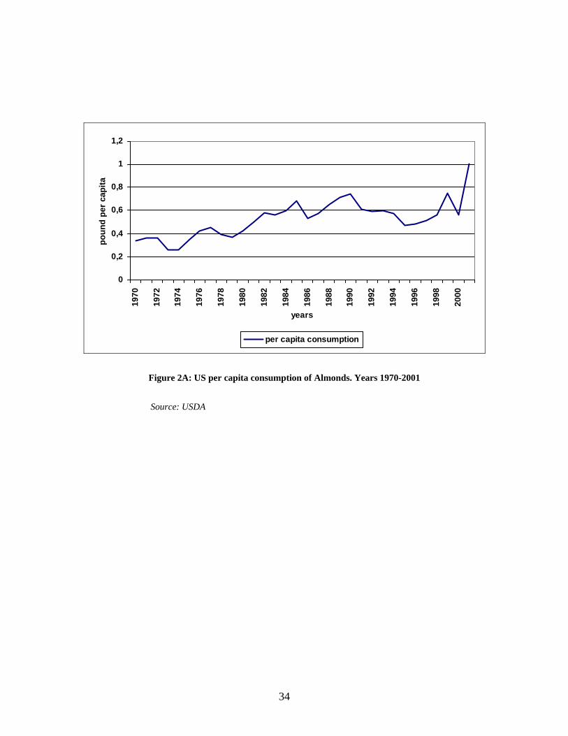
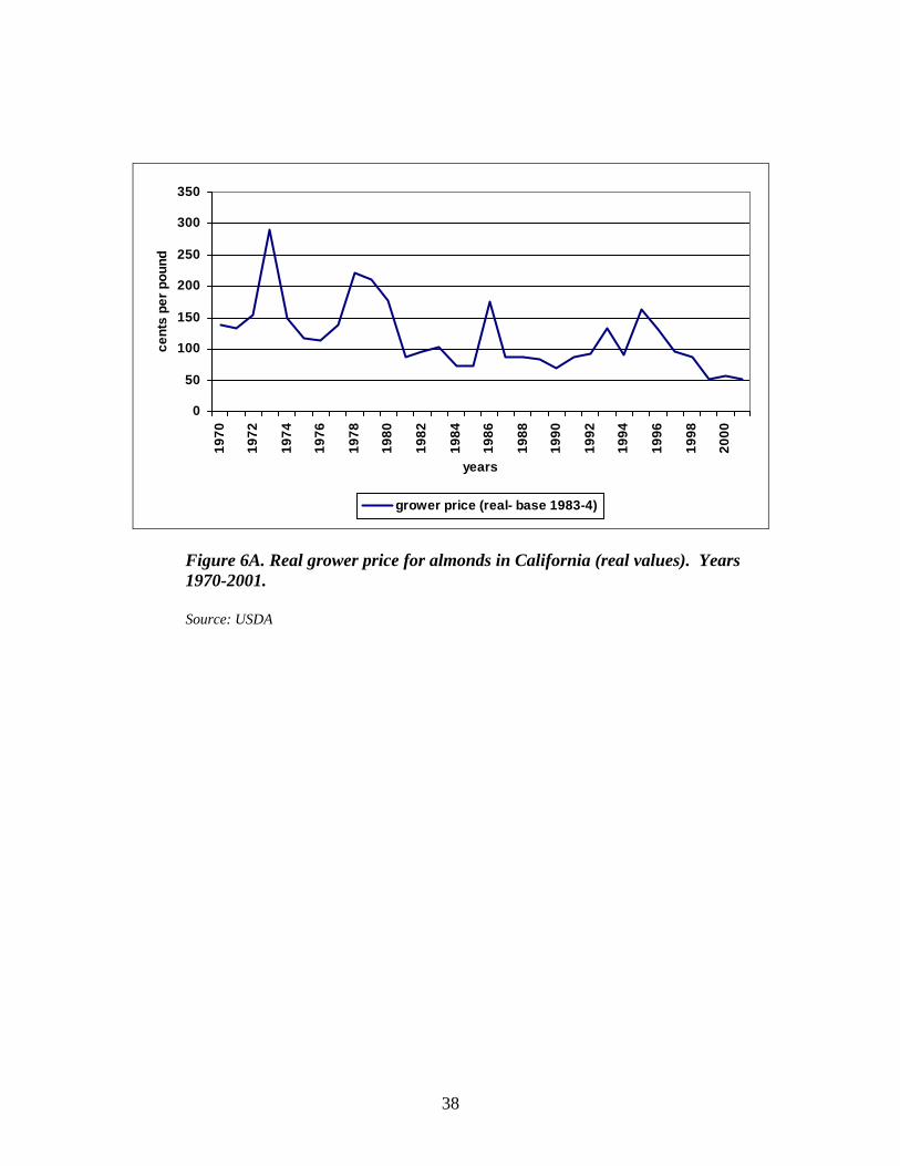
Figures 1A-6A in Appendix A provide a graphic overview of the domestic and
foreign markets for California almonds for the years 1970-2001 (USDA). The figures
contain information on marketable almond production, domestic per capita consumption,
export and import of almonds, acreage in California, yield per acre, and grower price
(nominal and real). A brief description of the almond industry will be given before the
empirical results are presented.
Production of almonds exhibit a well-known alternate bearing-year phenomenon,
that is, a high production year is followed immediately by a lower crop year and this
pattern continues. Exports of almonds over the years 1970-2001 have continued to
increase from less than 100 million pounds in 1970 to over 500 million pounds in 2001.
Per capita consumption of almonds has also continued to increase over the same time
period (Figure 2A). In 1970 per capita consumption of almonds were less than 0.4
pounds per capita and they increased to over 1 pound per capita in 2001. Acreage of
almonds in California rose steadily over the years 1970-2001 from less than 200 thousand
acres in 1970 to over 500 thousands acres in 2001. Per acre yield of almonds in
10
California exhibit a “see-saw” pattern, but the trend from 1970 has been increasing.
Nominal grower prices for almonds have been volatile over the 30-year period from 1970
to 2001 reaching a peak in 1995 of $2.50 per pound. The major policy implication from
Figure 6A; however, is that the real grower price, adjusted for inflation, has been steadily
decreasing over the 1970-2001 period. The 2001 real grower price of almonds was
barely over 50 cents per pound down from the peak real price of about $3.00 per pound in
1973. A causal glance at Figures 1A-6A in Appendix A indicates that the almond market
is continually changing and a lot of world marketing forces affect California’s production
and sales of almonds. Supply and demand models are developed and estimated for
almonds and the results are given in the next section.
Some theoretical and data issues must be addressed before the models and
estimations are presented. First, should a researcher use a singe-equation approach or a
system approach? In this report both approaches are presented, although single equation
estimations are usually considered to be less efficient. There are several reasons for
considering this model. Based on previous research work by the authors, alternative nuts
were found to be weak substitutes for almonds in the United States domestic market.
Similar results were also found by Alston et al (1995). Thus, the advantages of imposing
theoretical restrictions such as Slutsky symmetry conditions may be of little value in a
demand system or subsystem for nuts. In addition, retail prices for almonds do not exist
since they are used as ingredients in confectionaries. This has two important
implications. First, are the demand functions retail or farm-level demands? Wohlgenant
and Haidacher developed the theoretical relationships for the retail to farm linkages for a
complete food demand system. Their approach, however, assumes that both retail and
11

farm-level prices exist. In our case retail prices do not exist so we cannot employ their
approach. This limitation of the demand models needs to be considered when
interpreting the elasticity estimates. For example, farm-level own-price elasticities are
generally more elastic than retail own-price elasticities for food commodities. Second,
this may imply that nuts are not weakly separable from other food commodities.2 This
would rule out estimating a nut demand subsystem. The model that we employed uses
CPI to account for the prices of other food items and commodities.
Given the alternate bearing phenomenon of almonds, there is a demand for
consumption and a demand for storage. Alston et al (1995) did not find evidence of a
stockholding effect. Thus, we followed their approach and assume that the demand
function reflects consumption responses and not storage effects.
Finally, there is a calendar year versus a crop year problem involved with data
collection. Alston et al (1995), when they estimated the domestic demand for almonds,
used total availability (harvest received by handlers) minus US calendar year net exports
minus stocks carried out plus carryins as their dependent variable.
Single equation estimation: demand
Based on standard microeconomic theory, it is assumed that an individual
(representative) consumer behaves in such a way so as to maximize a well defined
quasiconcave utility function subject to a budget constraint (see, e.g., Deaton and
Muellbauer). The domestic aggregate demand for almonds can be written as
2 A reviewer questioned this assumption. Nuts appear to be not weakly separable from other food commodities since they are used as ingredients in other food products. One implication of weak separability is that demands for the weakly separable goods can be expressed as a function of prices within the group and group expenditure. In theory, for example, if the price of cakes decreases, then one would expect that the quantity demanded of cakes would increase and consequently the demand for nuts would increase violating one of the implications of weak separability. Weak separability of nuts could be tested in a demand system if data were available and thus, in principle, is a refutable hypothesis.
12

(3) ( , , ,t t t tQ f AP WP CPI PCIN= )t
where represents per capita almond consumption, represents the price of
almonds, denotes the price of walnuts, a possible substitute for almonds,
represents the consumer price index and captures the price of all other goods, and
denotes per capita income.
tQ tAP
tWP tCPI
tPCIN
3
With respect to functional forms for the almond demand equation, Box-Cox
flexible functional forms
10 1
t t tKK t
Q X Xλ λ λ
β β βλ λ λ
= + + + +ε (4)
were estimated by maximum likelihood procedures where λ can take on any value. All
of the estimations in the report are carried out using SHAZAM, version 10. The linear
and double logarithmic forms are special cases of the Box-Cox specification. The linear
and double-log functional forms in the almond demand equation were tested against the
more flexible Box-Cox functional form and in both cases the linear and double-log
specifications were strongly rejected. The values of the likelihood ratio statistics were
43.7 for the linear and 14.85 for double-log model. The chi-squared critical value with
one degree of freedom is 3.841 at the five percent significance level. Table 1 presents the
estimations. The homogeneity condition of degree zero in all prices and income (HOD)
does not hold globally in the Box-Cox specification unless the functional form is double
3 Demand theory describes the behavior of individual consumers. The estimations, however, use aggregate data over all consumers. This can result in aggregation biases. If the observations are time series of cross-section data on randomly selected households, then it can be shown that the aggregate coefficients converge, as the number of households (N) goes to infinity, in probability to the micro coefficients (Theil). The disturbance terms are heteroskedastic, however. White’s heteroskedastic-consistent standard errors for the estimated coefficients must be used. A recent excellent and thorough treatment of the conditions needed to avoid aggregation bias including exact aggregation and the distributional approach is given in Blundell and Stoker. They consider heterogeneity of consumers and distribution of income over time.
13

log.4 The linear, double-log, and Box-Cox estimated functional forms for almond
demand equations are presented in Table 3. In order to make the different models
comparable, homogeneity was imposed in the double-log models and the other models
were deflated by CPI.
4 The homogeneity condition is λ = 0 and Σβ j = 0 where the β 's are price and income coefficients; see Pope, et al. Linear specifications cannot be HOD by construction.
14

Table 3. Almond Demand Functions 1
Linear D. Log D. Log-A Box-Cox Box-Cox-A 3 2
_____________________________________________________________
AP 4 -0.0016 -0.480 -0.377 -0.2671 -2.386
p-value (0.0036) (0.0004) (0.0010) (0.0004) (0.0007)
elasticity -0.351 -0.480 -0.377 -0.477 -0.378
WP 5 0.0001 0.103 0.002 0.0436 -0.0267
p-value (0.3898) (0.5895) (0.9912) (0.5948) (0.9891)
elasticity 0.465 0.103 0.002 0.097 -0.002
PCIN 0.00001 0.870 0.973 0.2911 29.404
p-value (0.000) (0.0038) (0.0120) (0.0036) (0.0251)
elasticity 0.465 0.870 0.973 0.864 0.928
Const -0.403 -5.14 -5.429 -4.270 -78.211
p-value (0.000) (0.0042) (0.0068) (0.0319) (0.0394)
R2 0.62 0.74 0.80 0.74 0.82
lnL 28.484 14.051 17.66 35.91 40.239
λ 0.107 -0.340
ρ 0.49 0.56
1 is in pounds per capita, Q AP and WP are in cents per pound, and is in PCINdollars. 2,3 ”A” denotes autocorrelated correction models. 4,5 These are grower prices since retail prices do not exist.
15

The models were estimated using annual data from 1970 to 2001, a total of 32
observations. The Durbin-Watson values were 1.23 and 1.12 in the linear and double-log
functional forms. The critical values are 1.244 and 1.650 at the five percent significance
level, thus in the double-log and Box-Cox specifications the models were also estimated
with an AR(1) error process. The estimated autocorrelation coefficients were 0.49
(double-log) and 0.56 (Box-Cox) with an estimated asymptotic standard error of 0.15
(double-log) and 0.14 (Box-Cox). The estimated own-price elasticity of domestic
demand for almonds ranged from –0.48 to -0.35. The estimated elasticity was -0.38 in
the Box-Cox functional form with an AR(1) error process. The estimates were highly
significant with small p-values. Also, the estimated cross-price elasticity with walnuts
was positive in four of the five models, but none of the coefficients were statistically
significant; the smallest p-value being 0.39. The results confirm the absence of gross
substitution effects between almond and walnuts. All of the estimated income
coefficients were positive and ranged from 0.46 to 0.97 with small p-values. A
sequential Chow and Goldfeld-Quandt test was conducted to determine if any structural
changes had taken place during this period. No evidence was found of any structural
changes.
Additional models were estimated using the dependent variable, US total
consumption of almonds plus California exports minus US imports. The dependent
variable captures the international demand for US almonds as well as the domestic
demand. The ordinary least squares estimated double-log regression had an R2 of 0.92.
The estimated own-price elasticity of demand for almonds was -0.270 with an associated
16

p-value of 0.022. The estimated model had a positive time trend coefficient of 0.05 (p-
value =0.03) income elasticity was 2.10 with a p-value of 0.07.
Single equation estimation: supply
On the supply side, estimated almond acreage, yield, and marketable production
functions were estimated for the period 1970 to 2001. The almond acreage was estimated
using a partial adjustment model of the form:
( )( )
*
*1 1
1 t t
t t t t t
A P
A A A A
α β
γ ε− −
= +
− = − − + (5)
where equations (5) are the desired almond acreage and equation (6) is the actual acreage;
respectively. By substitution and some simplifications, the model can be estimated as:
( ) ( ) 11 1t tA P t tAγ α γ β γ −= − + − + +ε (6)
where At is the almond acreage (in acres), is the average real almond grower price per
pound over the previous eight years and, and
tP
ε t is an error term included to capture all
omitted factors that affect almond acreage.
This specification was chosen because it incorporates the behavior of producers
whom adjust their acreage when they realize that the desired acreage ( tA∗ ) differs from
the actual acreage the previous year ( 1tA − ). The adjustment coefficient, 1 γ− , indicates
the rate of adjustment of actual acreage to desired acreage. The partial adjustment model
is a model that captures producers’ behavior (see, e.g., Kmenta). Almond trees take
between five and six years to be fully productive. The acreage equation assumes a long-
run planning process based on past prices, which are considered a proxy of the farmers’
expectations about future prices.
17

The estimated acreage equation, with all variables expressed in logarithm form and
based on 1979-2001 annual observations, is:
1ˆln 0.32 0.12ln 0.97 ln
(0.31) (0.03) (0.04)t t tA P A −= − + + . (7)
The values in parentheses are standard errors. The coefficient of determination of the
regression is R2=0.97. The Durbin-h statistic is 1.40 which is asymptotically not
significant, thus there is no evidence of autocorrelation. The estimated short-run price
elasticity is 0.12 with an associated p-value of 0.0016. The estimated coefficient on
lagged acreage is 0.97 with an associated p-value of 0.0000. The estimated acreage
response equation provides empirical evidence that almond producers respond positively
to anticipated price increases in almonds.
The yield equation for almonds is:
21 2 1 3 4 5ln lnt t t t t tY P Rain T Tβ β β β β ε−= + + + + + (8)
where Y is almond yield in pounds per acre, is the real grower price of almonds in
cents per pound in the previous year,
t Pt −1
tRain is rainfall in inches in March, and T is a time
trend that is a proxy for technological change.
t
tT
The ordinary least squares estimated yield equation for almonds for the years
1971-2001 is (equation (9))
(9) 2
1ˆln 6.39 0.07 ln 0.20ln 0.05 0.001
(0.48) (0.09) (0.05) (0.01) (0.0003)t t t tY P Rain T−= + − + −
where the values in parentheses are standard errors. The estimated R2 is 0.68 which
indicates an adequate fit of the model with the data. All of the p-values for the estimated
coefficients are less than 0.10 except for one associated with lagged price. The
coefficient on lagged price is positive (0.07) but not significant. The coefficient on
18

March rainfall is negative (-0.20) reflecting the effect of rain on increased brown rot
disease and decreased pollination. The coefficient on the time trend is positive (0.05) and
significant indicating that, conditioned on all the other variables, yields are increasing
over the time period, 1971-2001. The coefficient on time squared is negative (-0.001)
and significant reflecting that the time trend is increasing at a decreasing rate. The
increasing trend can be due to technology and improvement of production practices. The
almond yield equation exhibits an alternate bearing phenomenon since the autocorrelation
was negative ( ˆ 0.38ρ = ) with an asymptotic t-value of 2.26.5 The model was estimated
using the autocorrelation method of Pagan in SHAZAM. The other autocorrelation
methods, ML and Cochrane–Orcutt gave similar results.
Finally, a production function for almonds was developed and estimated. The
model is:
1 2 1 3 4 1t tQln ln ln lnt t tQ P Rainβ β β−= + + +
1tP−
t
β ε− + (10)
where is California almond production in millions of pounds, represents the
lagged price of almonds in cents per pound,
tQ
Rain
1tQ −
represents March rainfall in inches,
and denotes lagged production. The model is a partial adjustment model and
includes the effect of alternate crop years and weather. As in the yield equation, the
alternative bearing phenomenon is captured by a negative autocorrelation coefficient.
The estimation of the model, correcting for autocorrelation, is
5 Several methods were used to capture the alternate-year yield phenomenon. For example, a dummy variable was added to the function with zero values for low-yield years and ones for high-yield years. Due to weather conditions and new varieties of trees that started bearing, the data exhibits a high-low pattern for a number of years followed by two high-yield years in a row or two low-yield years in a row. The high-low pattern continues for a few years but the pattern may be reversed. History then repeats itself. It is difficult to capture these phenomena with a dummy variable in the systematic part of the equation. This
19

1ˆln 0.44 0.19ln 0.20ln 0.97 ln
(1.24)(0.15) (0.07) (0.11) t t tQ P Rain−= − + − + 1tQ −
(11)
where the numbers in parentheses are estimated standard errors. The R2 of the model is
0.71. The elasticity of production with respect to the lagged own price (for given values
of the production in the previous year, the weather conditions and the alternate crop
years) is 0.19 but not significant (p-value= 0.20). The coefficient on March rainfall is
negative as explained above and the estimated coefficient on lagged production is
positive and highly significant. The alternate crop pattern was capture by a negative
autocorrelation coefficient of -0.55 with an associated asymptotic t-value of 3.74.6
WALNUTS
Data for the years 1970-2001 are presented in Appendix B for walnuts. California
marketable production, total domestic consumption, exports and imports, per capita
consumption, acreage, yield, and grower prices, both nominal and real for walnuts are
given in Figures 1B-6B in Appendix B. An overview of the walnut industry can be seen
by an examination of the Figures. Marketable production of walnuts has slowly
increased from just below 100 million pounds in 1970 to over 250 million pounds in
2001. Exports of walnuts exhibit a similar pattern of that to production (see Figure 1B in
Appendix B). Per capita consumption of walnuts has remained relatively stable at 0.4
pounds over the period 1970-2001 (Figure 2B). Acreage has slowly increased over the
period starting with about 150 thousand acres in 1970 to about 200 thousand in 2001.
was not the case with walnuts where the alternate pattern was consistent throughout the sample period. See the patterns in the data for almond yields, walnut yields, and walnut production in Appendix C. 6 Alternative functional forms of the production function were estimated including a Box-Cox specification, models with moving average error schemes, etc. The Box-Cox functional form yielded a price elasticity of 0.29 and a model estimated with a moving average error term yielded a slightly lower price elasticity estimate of 0.23.
20

Yields of walnuts are more volatile over the period than acreage but with a steady trend
upward over the period 1970-2001 (Figure 4B). Real grower prices have decreased over
the period from 1970 to 2001 (Figure 6B). Real grower prices reached a peak in about
1978 of $2.00 per pound and have declined ever since to about 60 cents per pound in
2001.
Demand, acreage, yield, and production equations were estimated for walnuts
using annual data from 1970 to 2001. The United States domestic demand for walnuts is
estimated and reported first.
The model for US per capita consumption of walnuts is
(13) ( , , ,t t t tQ f AP WP CPI PCIN= )t
tQ tAP
tI
t
where represents per capita walnut consumption in pounds, represents the price
of almonds in cents per pound where almonds are a possible substitute for walnuts,
denotes the price of walnuts in cents per pound, CP represents the consumer price
index and captures the price of all other goods, and denotes per capita income in
dollars.
tWP
PCIN
The restriction of homogeneity of degree zero in all prices and income was
imposed. When the model for all the years, 1970 to 2001, was estimated by ordinary
least squares, the Durbin-Watson value was small (0.796) indicating a possible
misspecified model. Consequently, sequential Chow and Goldfeld-Quandt tests were
performed and they indicated a structural break in 1983. Two demand functions were
estimated, one using data from 1971 to 1983 and one employing data from 1983 to 2001.
The estimated models, double-log and Box-Cox functional forms, are presented in Table
4.
21

Table 4. Walnut Demand Functions
Pre 1983 Post 1983
Double Log Box-Cox Double Log Box-Cox
AP -0.210 -0.449 -0.082 -0.19E-06
p-value (0.039) (0.136) (0.325) (0.667)
elasticity -0.210 -0.197 -0.082 -0.023
WP -0.284 -0.825 -0.267 -0.26E-07
p-value (0.068) (0.113) (0.063) (0.051)
elasticity -0.284 -0.266 -0.267 -0.251
CPI -1.039 -1.435 -0.633 -0.61E-05
p-value (0.029) (0.612) (0.414) (0.307)
elasticity -1.039 -0.677) -0.633 -0.807
PCIN 1.534 5.349 -0.983 0.10E-09
p-value (0.007) (0.339) (0.201) (0.398)
elasticity 1.039 1.207 -0.983 0.427
Constant -7.361 -17.519 -4.50 -0.333
p-value (0.005) (0.304) (0.207) (0.000)
R2 0.759 0.763 0.705 0.726
DW 2.563 2,43 2.069 2.507
lnL 15.988 26.029 25.492 44.217
λ 0 -0.15 0 2.06
22
The 2R values range from 0.71 to 0.76. The fit of the models to the data was not
as good as for the almond demand equations. The Durbin-Watson statistics did not
indicate any problems with autocorrelation. The estimated own-price elasticity of
demand for walnuts ranged from –0.266 to -0.284 for the time period prior to 1983 and
from -0.251 to -0.267 after the year 1983. The p-values were 0.068 (pre 1983) and 0.63
(post 1983) for the double-log models and 0.113 (pre 1983) to 0.051 (post 1983) for the
Box-Cox functional forms. The Box-Cox equation post 1983 was estimated with a time
trend. Its estimated coefficient was -0.03 with an associated p-value of 0.014. Three of
the four estimated income elasticities were positive with only the post 1983 for the
double-log specification negative (-0.983). Only one of the estimated almond cross-price
elasticities was significant at any reasonable level. Thus, the sample evidence finds little
substitution effects between almonds and walnuts. Based on the sample evidence the
estimated own-price elasticity of demand for walnuts is inelastic.
What are some economic factors that can explain the structural break around
1982-83? From Figure 6B, real walnut prices dropped dramatically in 1983. There was a
large supply of walnuts that year and inventory levels increased significantly. In
addition, the United States imposed a tariff on pasta and Italy, one of the largest
importers of U.S. walnuts, retaliated by placing an embargo on U.S. walnuts. Exports
dropped causing increases in inventory levels.
Another model was estimated where the dependent variable was US total
consumption of walnuts plus California exports minus US imports. The dependent
variable captures domestic plus net export demand. Again, sequential structural tests
indicated a structural break around 1983. The results from this estimated equation
23

yielded a total own-price elasticity of demand for walnuts of –0.354 prior to 1983 and an
estimated value of –0.061 after 1983. The estimated coefficient of determination for this
equation was 0.923. The wide difference between the estimated own-price elasticities of
demand between the two time periods may be due, in part, to structural changes
mentioned above. The primary policy implications are that the demand for walnuts is
inelastic with little evidence that almonds are an important substitute for walnuts.
On the supply side, acreage, yield, and production equations were estimated for
walnuts, using a partial adjustment model. The estimated acreage equation is
2
1ˆln 2.90 0.02ln 0.00 0.00 0.74ln
(1.16) (0.01) (0.00) (0.00) (0.10)t t t t tA P T T A −= + + + + (14)
where represents acreage of walnuts in acres, P denotes walnuts grower prices of
walnuts in cents per pound and T is a time trend. Values in parentheses represent
standard errors. The estimated coefficient of determination,
At
R2 , was 0.953. The
estimated short-run elasticity of acreage with respect to price is 0.02, which implies that
acreage is inelastic with respect to the current price. The estimated lagged acreage
coefficient was 0.74 and highly significant indicating a partial adjustment by producers of
walnut acreage over time. Figure 6 charts the actual acreage of walnuts to the predicted
values.
24
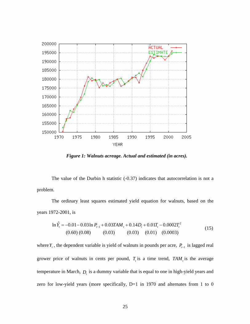
Figure 1: Walnuts acreage. Actual and estimated (in acres).
The value of the Durbin h statistic (-0.37) indicates that autocorrelation is not a
problem.
The ordinary least squares estimated yield equation for walnuts, based on the
years 1972-2001, is
21
ˆln 0.01 0.03ln 0.03 0.14 0.01 0.0002 (0.60) (0.08) (0.03) (0.03) (0.01) (0.0003)
t t t t tY P TAM D T−= − − + + + − tT (15)
whereY , the dependent variable is yield of walnuts in pounds per acre, is lagged real
grower price of walnuts in cents per pound, T is a time trend, TA is the average
temperature in March,
t 1tP−
t Mt
tD is a dummy variable that is equal to one in high-yield years and
zero for low-yield years (more specifically, D=1 in 1970 and alternates from 1 to 0
25

throughout the sampling period) and is included to capture the alternate yield-year
phenomenon. The coefficient of determination is 0.72. The Durbin-Watson calculated
value of 1.78 does not support evidence of negative correlation. The “see-saw” pattern
exhibited by walnut yields is more consistent that than for almond yields and thus the
dummy variable included in the systematic part of the equation picks up the alternative
bearing phenomenon (see Appendix C). The estimated coefficient on D is positive and
highly significant as expected and the coefficient on March temperature is positive as
expected but not significant. There is a little evidence of a positive time trend. The
lagged price coefficient is unexpectedly negative but not significant.
The final estimation for walnuts consists of estimating a production function for
the years 1971-2001. The estimated production function, corrected for autocorrelation,
is:
1 1ˆln 3.52 0.003ln 0.03 0.23 0.69ln
(1.84) (0.06) (0.02) (0.07) (0.13)t t t tPR P TAM D PRt− −= + + + + (16)
where the dependent variable, , is walnut production in millions of pounds, tPR 1tP− is
walnut price in cents per pound, TA is the March temperature, and is a dummy
variable that takes on the values of 1 and 0 and accounts for the alternate year production
phenomenon. The R
Mt tD
2 of the regression is 0.82. The estimated autocorrelation coefficient
is -0.47 with as asymptotic t-value of 2.60. The alternate year dummy coefficient is
positive and highly significant as expected is picking up all the alternate production year
effect. The estimated coefficient on lagged walnut price is positive but insignificant and
the estimated coefficient on lagged production is positive and significant. The positive
sign on March temperature is as expected.
26

SUR Estimation
The results of the estimations suggest that walnuts and almonds cannot be
considered as close substitutes or complements because the cross-price elasticities were
not significantly different from zero. However, the possible relations across the two
markets can be explored using a demand system of seemingly unrelated equations (SUR).
In this system, correlation in the errors across equations is assumed. Some of the same
omitted factors may influence both almond and walnut demands.
The equations are estimated using an iterative SUR procedure to achieve
efficiency. Also the properties of symmetry and zero homogeneity were imposed. The
estimation of the system (eq. 17) is:
ln 4.17 0.14ln 0.20ln 0.48ln 0.82ln 0.19 0.07 (3.57) (0.14) (0.08) (0.07) (0.78) (0.01) (0.08)ln 5.45 0.20ln
W W At t t t t t t
At
D
PC = − − 0.18ln 0.67 ln 1.05ln (1.64) (0.08) (0.17) (0.40) (0.29)
A Wt t t tP P CPI PCIN− − +
PC P P CPI PCIN T= − − − − + − −
where numbers in parentheses are standard errors, PCW and PC A are the per-capita
consumption of walnuts and almond, respectively. PC w and PC A are grower nominal
prices of walnuts and almonds, respectively, is a dummy variable that takes on the
value of zero prior to 1983 and the value of one after 1983. The remaining variables are
as defined above except per capita income is also expressed in nominal terms. The
system
tD
2R is equal to 0.81. The estimated own-price elasticity of walnuts is -0.14 and
that of almonds -0.20; with only the estimated own-price elasticity of almonds being
highly significant. The estimated income elasticity for walnuts is 0.82 and that of
almonds is 1.05.
27

Some Policy Implications
Based on the models estimated for almonds and walnuts the own-price elasticity
of US domestic demand for almonds was found to be between –0.35 and -0.48.. These
estimates are inelastic and imply that almond producers are vulnerable to large swings in
prices of almonds due to supply shifts. Similar estimates of the own-price elasticity of
US domestic demand for walnuts were obtained. The estimated own-price elasticities for
walnuts ranged from –0.25 to –0.28. Walnut producers face the same marketing situation
as almond producers, that is, prices of walnuts fluctuate widely due to shifts in the supply
function of walnuts.
The estimated acreage response equation for almonds indicated that producers
respond positively to lag prices. The estimated short-run price elasticity of acreage for
almonds was 0.12 and significant. This is relatively small but does indicate that
producers are responsive to increases in prices over time. For walnuts the estimated
short-run price elasticity of acreage was 0.02 and significant. Again, the value is small
but positive.
The estimated yield equations for both almonds and walnuts reflected a
significant alternate-year phenomenon. For almonds the phenomenon was capture by a
significant and negative autocorrelation coefficient. For walnuts it was captured by a
dummy variable. Yields for almonds are significantly affected by a time trend. Yields of
almonds are increasing over the time period 1979-2001, based on the estimated yield
equation. For walnuts, yields were positively affected by temperature in March and a
time trend, but neither coefficient was significant.
28
A SUR demand system was estimated for walnuts and almonds. The domestic
own-price elasticity of demand for walnuts was estimated to -0.14 and that of almonds -
0.20 with almonds being significant. The estimated income elasticity of demand for
walnuts was 0.82 and that for almonds was 1.05 with the estimated income elasticity in
the almond equation being significant. The evidence does not support gross substitution
between almonds and walnuts.
The primary policy implication based on these results is that almond and walnut
producers are facing an inelastic domestic demand for their products. Combine this with
the volatility of the supply function due to temperature and rainfall changes, wide
variations in prices exist which lead to wide variations in profits from year to year.
Storage, improved technology, and an expanding export market are factors that may
mitigate the volatile market conditions facing US producers of almonds and walnuts.
29

References
Alston, J., H. Carman, J. Christian, J. Dorfman, J-R. Murua, and R. Sexton, “Optimal
Reserve and Export Policies for the California Almond Industry: Theory,
Econometrics and Simulations.” Giannini Foundation Monograph, No. 42,
February 1995.
Alston, J., J. Chalfant, J. Christian, E. Meng, and N. Piggott, “The California Table Grape
Commission’s Promotion Program: An Evaluation.” Giannini Foundation
Monograph, No. 43, November 1997.
Alston, J., H. Carman, J. Chalfant, J. Crespi, R. Sexton, and R. Venner, “The California
Prune Board’s Promotion Program: An Evaluation.” Giannini Foundation
Research Report, No. 344, March 1998.
Blanciforti, L., R. Green, and G. King, “U.S. Consumer Behavior Over the Postwar
Period: An Almost Ideal Demand System Analysis.” Giannini Foundation
Monograph, No. 40, August 1986.
Blundell, R. and T. Stoker, “Heterogeneity and Aggregation”, Journal of Economic
Literature, 43(June 2005):347-391.
Carman, H. and R. Green, “Commodity Supply Response to a Producer Financed
Advertising Program: The California Avocado Industry” Agribusiness: An
International Journal, 1993, 605-621.
Goodwin, B. and G. Brester, “Structural Change in Factor Demand Relationships in the
U.S. Food and Kindred Products Industry.’ American Journal of Agricultural
Economics 77(1995):69-79.
30

Green, R., H. Carman, and K. McManus, “Some Empirical Methods of Estimating
Advertising Effects in Demand Systems: An Application to Dried Fruits.”
Western Journal of Agricultural Economics 16(1):63-71.
Green, R., “Demand for California Agricultural Commodities.” Update Vol. 2, No. 2,
Winter 1999.
Johnston, W. and A. McCalla. “Whither California Agriculture: UP, Down, or Out?
Some Thoughts about the Future.” Giannini Foundation Special Report 04-1,
August 2004.
Kinney, W., H. Carman, R. Green, and J. O’Connell, “An Analysis of Economic
Adjustments in the California-Arizona Lemon Industry.” Giannini Foundation
Research Report, No. 337, April 1987.
Kmenta, J. Elements of Econometrics, 2nd ed., Macmillan Pub. Co., New York, 1986.
Knapp, K. and K. Konyar, “Perennial Crop Supply Response: A Kalman Filter
Approach.” American Journal of Agricultural Economics, 73(1991):841-849.
Morrison Paul, C. and J. MacDonald, “Tracing the Effects of Agricultural Commodity
Prices and Food Costs.” American Journal of Agricultural Economics
85(2003):633-646.
Nuckton, C., “Demand Relationships for California Tree Fruits, Grapes, and Nuts: A
Review of Past Studies”, Giannini Foundation Special Publication No. 3247,
August 1978.
Nuckton, C., “Demand Relationships for Vegetables: A Review of Past Studies”,
Giannini Foundation Special Report 80-1, 1980.
31

Pope, R., R. Green, and J. Eales, “Testing for Homogeneity and Habit Formation in a
Flexible Demand Specification of U.S. Meat consumption” American Journal of
Agricultural Economics 62(1980): 778-784.
Renwick, M. and R. Green, “Do Residential Water Demand Side Management Policies
Measure Up? An Analysis of Eight California Water Agencies” Journal of
Environmental Economics and Management 40(2000):37-55.
Sexton, R. and M. Zhang, “A Model of Price Determination for Fresh Produce with
Application to California Iceberg Lettuce.” American Journal of Agricultural
Economics 78(1996):924-34.
Wohlgenant, M. and R. Haidacher, “Retail to Farm Linkage for a Complete Demand
System of Food Commodities”, USDA, ERS, Technical Bulletin No. 1775, 1989.
Zellner, A. “Philosophy and Objectives of Econometrics”, Journal of Econometrics,
2006.
32
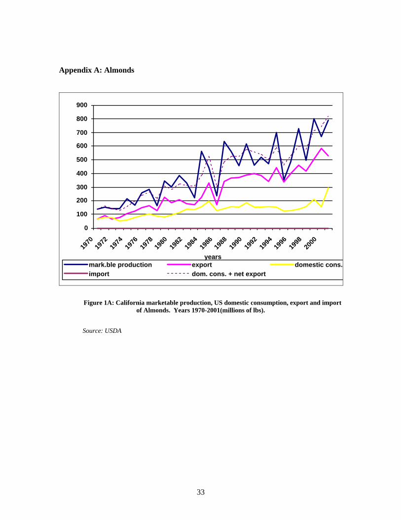
Appendix A: Almonds
0
100
200
300
400
500
600
700
800
900
1970
1972
1974
1976
1978
1980
1982
1984
1986
1988
1990
1992
1994
1996
1998
2000
yearsmark.ble production export domestic cons.import dom. cons. + net export
Figure 1A: California marketable production, US domestic consumption, export and import
of Almonds. Years 1970-2001(millions of lbs).
Source: USDA
33
0
0,2
0,4
0,6
0,8
1
1,219
70
1972
1974
1976
1978
1980
1982
1984
1986
1988
1990
1992
1994
1996
1998
2000
years
poun
d pe
r cap
ita
per capita consumption
Figure 2A: US per capita consumption of Almonds. Years 1970-2001
Source: USDA
34

0
100
200
300
400
500
600
1970
1972
1974
1976
1978
1980
1982
1984
1986
1988
1990
1992
1994
1996
1998
2000
years
thou
sand
s of
acr
es
acreage
Figure 3A: Acreage of almonds in California. Years 1970-2001 Source: USDA
35

0
50
100
150
200
250
300
1970
1972
1974
1976
1978
1980
1982
1984
1986
1988
1990
1992
1994
1996
1998
2000
years
cent
s pe
r pou
nd
grower price (nominal)
Figure 4A: Grower price for almonds in California (nominal values). Years 1970-2001
Source: USDA
36

0200400600800
100012001400160018002000
1970
1972
1974
1976
1978
1980
1982
1984
1986
1988
1990
1992
1994
1996
1998
2000
years
poun
ds p
er a
cre
yield
Figure 5A: Yield of almonds in California. Years 1970-2001
Source: USDA
37
0
50
100
150
200
250
300
350
1970
1972
1974
1976
1978
1980
1982
1984
1986
1988
1990
1992
1994
1996
1998
2000
years
cent
s pe
r pou
nd
grower price (real- base 1983-4)
Figure 6A. Real grower price for almonds in California (real values). Years 1970-2001. Source: USDA
38

Appendix B: Walnuts
0
100
200
300
400
500
600
700
800
900
1970
1972
1974
1976
1978
1980
1982
1984
1986
1988
1990
1992
1994
1996
1998
2000
years
mill
ion
of p
ound
s
marketable production importexport domestic consumptiondomestic cons.+export-import
Figure 1B: California marketable production, US domestic consumption, export and import of Walnuts. Years 1970-2001
Source: USDA
39

0
0.2
0.4
0.6
0.8
1
1.2
1970
1972
1974
1976
1978
1980
1982
1984
1986
1988
1990
1992
1994
1996
1998
2000
years
poun
d pe
r cap
ita
per capita consumption
Figure 2B: US per capita consumption of Walnuts. Years 1970-2001
Source: USDA
40

0
100
200
300
400
500
600
1970
1972
1974
1976
1978
1980
1982
1984
1986
1988
1990
1992
1994
1996
1998
2000
years
thou
sand
s of
acr
es
acreage
Figure 3B: Walnut acreage in California. Years 1970-2001
Source: USDA
41

0200400600800
100012001400160018002000
1970
1972
1974
1976
1978
1980
1982
1984
1986
1988
1990
1992
1994
1996
1998
2000
years
poun
ds p
er a
cre
yield
Figure 4B: Per acre yield of Walnuts in California. Years 1970-2001
Source: USDA
42

0
50
100
150
200
250
300
1970
1972
1974
1976
1978
1980
1982
1984
1986
1988
1990
1992
1994
1996
1998
2000
years
cent
per
pou
nd
grower price (nominal)
Figure 5B: Grower price for walnuts in California (nominal values). Years 1970-2001 Source: USDA
43

0
50
100
150
200
250
300
350
1970
1972
1974
1976
1978
1980
1982
1984
1986
1988
1990
1992
1994
1996
1998
2000
years
cent
per
pou
nd
grower price (real- base 1983-4)
Figure 6B: Real grower price for walnuts in California (real values). Years 1970-2001
Source: USDA
44
APPENDIX C: Almond Yields, Walnut Yields, and Walnut Production, 1970-2001
________________________________________________________________________
Year Almond Yields Walnut Yields Walnut Production
(Pounds/Acre) (Pounds/Acre) (Millions Lbs)
1970 877 740 108000 1971 863 900 135000 1972 759 740 116000 1973 726 1100 174000 1974 995 950 155000 1975 748 1190 198000 1976 1100 1080 183000 1977 1130 1090 192000 1978 588 880 160000 1979 1160 1160 208000 1980 985 1100 197000 1981 1250 1290 225000 1982 1250 1310 234000 1983 1020 1130 199000 1984 672 1200 213000 1985 1550 1220 219000 1986 1140 1000 180000 1987 601 1400 247000 1988 1580 1180 209000 1989 1410 1280 229000 1990 1190 1250 227000 1991 1610 1430 259000 1992 1210 1140 203000 1993 1370 1410 260000 1994 1190 1230 232000 1995 1700 1210 234000 1996 885 1080 208000 1997 1190 1390 269000 1998 1720 1180 227000 1999 1130 1480 283000 2000 1130 1240 239000 2001 1740 1560 305000 _______________________________________________________________
Source: USDA.
45

ALFALFA AND COTTON
Introduction
Historically, from 1950-2002, alfalfa and cotton have been among California’s
top commodities in terms of total value (Johnston and McCalla). In 1950 cotton was
ranked third in terms of value of production in California with a value of $202 million.
By 2001, cotton had slipped to the eighth most valuable commodity in California in value
of production. The trend has been downward during the period 1950-2002. Hay (85%
alfalfa) was ranked fifth in 1950 in California with a value of production of $121 million.
In 2001, hay was ranked seventh in value of production just ahead of cotton.
Models are developed for California alfalfa and cotton acreage, production, and
consumption. Both single equation and systems of equations are estimated. The data
consist of 33 annual observations from 1970 to 2002. In some models, there were
slightly fewer observations due to lags in the specifications. A brief description of the
alfalfa market is given prior to reporting the estimations of the models. In addition, some
issues related to the nature of the data are discussed.
Alfalfa Alfalfa hay acreage in California has averaged about a million acres per year
during the past 30 years (Figure 1A). Alfalfa contributes about 85 percent of the value of
all hay production in California. Alfalfa is influenced by profitability of alternative
annual crops such as cotton, tomatoes, trees, and vines. The demand for alfalfa hay is
determined to a large degree by the size of the state’s dairy herd, which consumes about
70 percent of the supply. Horses consume about 20 percent. Alfalfa is a perennial crop
with a three to five-year economic life. Since it is a water intensive crop, its profitability
1

is strongly influenced by water and water costs. In addition, alfalfa is important in crop
rotations because of its beneficial effects on the soil (Johnston, p. 87).
Alfalfa production in California has been increasing annually since the mid
nineties (Figure 2A). It reached a peak in 2002 at 8.1 million tons. The increase in
production has been primarily due to the upward trend in yields (Figure 3A) and not to
increases in acreage. Alfalfa real grower price in California, using a 1983/84 base, has
exhibited a downward trend since the early eighties (Figure 6A). In 2002 the real grower
price was about $60 per ton.
Model for Alfalfa Acreage A partial adjustment model of alfalfa acreage is based on the following equation:
0 1 1 2 3 4 5
6 7
ln ln ln ln *ln*ln *ln
t t t t t t
t t t t t
A A P risk crit crit Acrit P crit risk
1tβ β β β β ββ β ε
− −= + + + + ++ + +
(1)
where represents planted alfalfa acreage in thousands of acres, is alfalfa price per
ton, is the variability in alfalfa price (measured by the standard deviation), and
is a dummy variable identifying the critical years for water scarcity (i.e., the year
when the Four river index fell below the value of 5.4). The is an index
to measure the water availability in California based on four river flows. The higher the
value the more water available. Two interaction terms are also included in the model to
capture the effects of water scarcity on prices and risk.
At Pt
riskt
critt
Four river index
The results of the estimation are (equation 2):
1 1ˆln 4.08 0.67 ln 0.35ln 0.61ln 23.80 2.56 *ln
(1.66) (0.17) (0.16) (0.27) (10.95) (1.26) +0.31 ln 0.67 ln
t t t t t t
t t t t
A A P risk crit crit A
crit P crit risk
− −= + + − − +
∗ + ∗ (0.59) (0.58)
t
(2)
2

where the numbers in parentheses are estimated standard errors. The estimation supports
the hypothesis that alfalfa acreage is influenced by prices, ceteris paribus. The short-run
price elasticity of acreage is 0.35 and significant when ample water is available and 0.66
when there is a shortage of water. Acreage increases with price expectations and
decreases with increases in perceived risk, as anticipated. Also the availability of water
has a significant impact on acreage. An F-test on the joint significance of the variable
“crit” and its cross products allows us to reject the null hypothesis of no impact at a 90%
confidence level (p-value: 0.0787). The signs of the coefficients are consistent with a
reduction of planting of new crop acreage during critical years of water scarcity.
Furthermore, the estimated coefficient on lagged acreage is 0.67 and significant
supporting the partial adjustment framework.
The regression R2 is 0.847, indicating a good fit. The Durbin h test indicates that
there is no autocorrelation in the disturbance terms. Graph 1 depicts the actual and
estimated values for alfalfa acreage:
3

Graph 1: Actual and estimated values of alfalfa acreage (in thousands of acres).
Model for Alfalfa Yield
Alfalfa yield is modeled by the following equation:
lnYt = β0 + β1 ln Pt−1 + β3 lnCPt−1 + β4 FRIt + β5Dt + ε t (3)
where is alfalfa yield in tons, is lagged alfalfa price per ton, CP is lagged cotton
price $/lb.(the rotation crop), is the value of the Four River Index (approximating
the availability of water) and is a dummy variable identifying the year 1978 as an
outlier. The model includes a moving average component of order two.
Yt Pt−1 t−1
FRIt
Dt
The estimated yield equation is:
(4) 1 1ˆln 1.31 0.08ln 0.14ln 0.01 0.12
(0.02)(0.00) (0.01) (0.00) (0.03)t t t tY P CP FRI D− −= + − + − t
where numbers in parentheses are standard errors. The estimated equation indicates that
yields respond positively to changes in prices and water availability. Both of these
4

estimated coefficients are highly significant. Alfalfa yields are negatively related to last
year’s cotton price since they compete for the same irrigated land.. The estimated
coefficient is also highly significant. The 1978 dummy coefficient is negative and
significant as expected as it was a major drought year. Including a dummy variable for
one year is equivalent to eliminating the 1978 observation.
The regression exhibits a good fit (R2 is 0.93) and the tests ruled out autocorrelation
(the Durbin-Watson statistics is 2.00) in the disturbance terms. . Graph 2 describes the
actual and estimated alfalfa yields.
Graph 2: Actual and estimated values of alfalfa yield (tons/acre).
Production The estimated alfalfa production equation (Table 1) is presented in tabular form in
order to better facilitate interpretations of estimated coefficients:
5

Table 1. Alfalfa Production Equation
Variable Coefficients Standard errors
Constant 4.87 1.98 Lag of Log Production 0.69 0.21 Lag of Log Alfalfa Price 0.44 0.17 Lag of Log Alfalfa Risk -0.75 0.28 Lag of Log Cotton Price -0.07 0.03 Dummy for critical years -12.07 5.77 Crit*Lag of Log Production 1.33 0.74 Crit*Lag of Log Alfalfa Price -3.87 1.27 Crit*Lag of Log Alfalfa Risk 3.61 1.02 Crit*Lag of Log Cotton Price 0.13 0.08 Dummy for outlier (1978) -0.08 0.03
The estimated own-price elasticity is 0.44 and significant at the usual 5%
significance level which suggests that alfalfa production is relatively inelastic. Alfalfa
production is negatively related to risk (price volatility) and cotton prices. Both
estimated coefficients are significant. Water shortages have a negative impact on alfalfa
production (see the estimated coefficient of -12.07 on the dummy variable for critical
years and is significant).
The regression R2 is 0.817. The Durbin h statistics (-0.62) indicates that there is
no problem with autocorrelation in the errors. Graph 3 plots actual and estimated values
of alfalfa production.
6
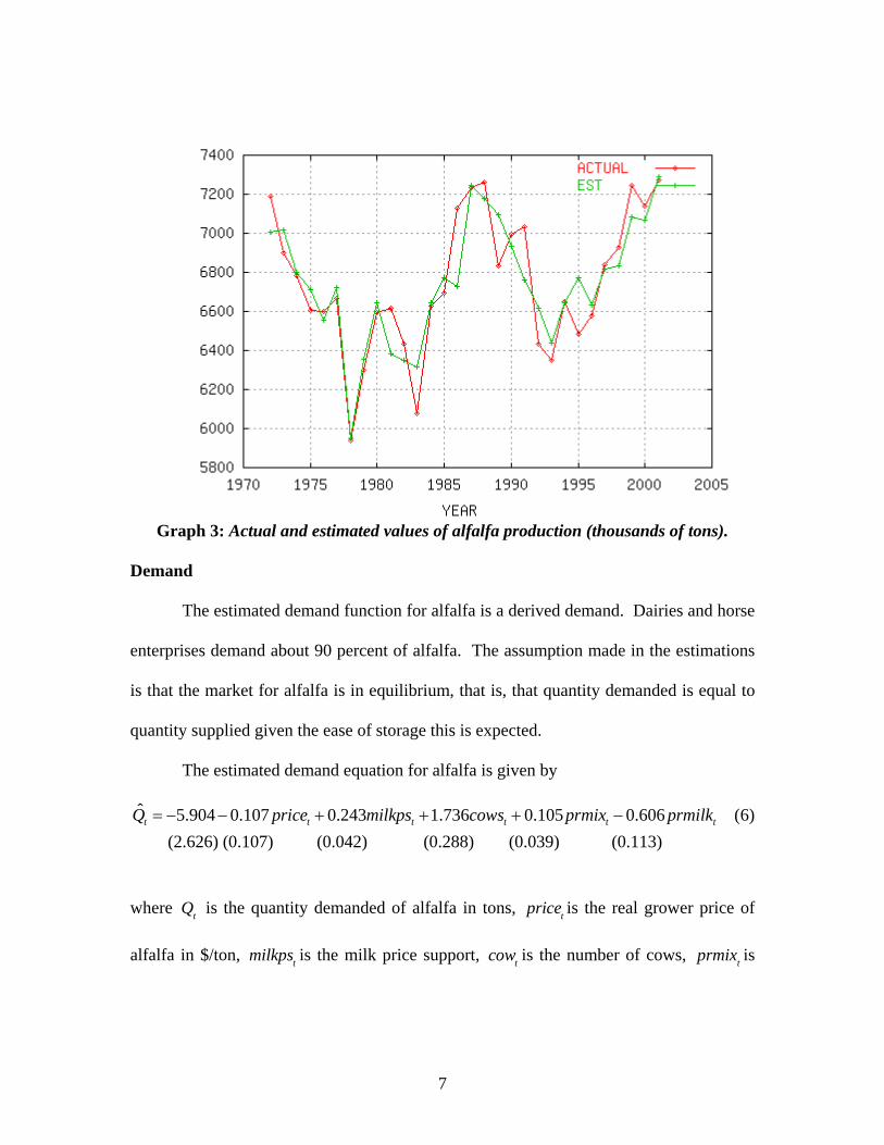
Graph 3: Actual and estimated values of alfalfa production (thousands of tons).
Demand
The estimated demand function for alfalfa is a derived demand. Dairies and horse
enterprises demand about 90 percent of alfalfa. The assumption made in the estimations
is that the market for alfalfa is in equilibrium, that is, that quantity demanded is equal to
quantity supplied given the ease of storage this is expected.
The estimated demand equation for alfalfa is given by
ˆ 5.904 0.107 0.243 1.736 0.105 0.606 (6) (2.626) (0.107) (0.042) (0.288) (0.039) (0.113)
t t t t tQ price milkps cows prmix prmilk= − − + + + − t
where is the quantity demanded of alfalfa in tons, is the real grower price of
alfalfa in $/ton, is the milk price support, is the number of cows, is
Qt pricet
milkpst cowt prmixt
7
the price of a combination of corn and soybeans, and is the real price of milk.
All variables are expressed in logarithmic form.
prmilkt
The coefficient of determination, , indicates a good fit of the model
with the data. The own-price elasticity of demand is -0.107 which is inelastic, but not
statistically significant. The estimated coefficient of milk support price is 0.243 implying
that the quantity demanded of alfalfa increases as the support price of milk increases.
The estimated coefficient on real price of milk is negative. The coefficient on the number
of cows is positive and statistically significant. This is reasonable given that about 70%
of the demand for alfalfa is from dairies. All of the coefficients in the demand equation
are statistically significant at the five percent level of significance except for own price.
R2 = 0.888
System for Alfalfa A three-equation system for alfalfa was developed and estimated. Iterative three-
stage least squares are used to estimate a model consisting of acreage, production, and
demand relationships for alfalfa. We assume that the market for alfalfa is in equilibrium,
that is, that quantity demanded is equal to production. We further assume that stocks are
included in the demand for alfalfa. Thus, the three endogenous variables are: acreage,
production, and alfalfa price. The estimators will be asymptotically efficient given that
the model is specified correctly. The gain in efficiency is due to taking into account the
correlation across equations. And three-stage least squares will purge (asymptotically)
the correlation that exist between endogenous variables on the right hand side of the
equations in the model with the error terms.
The estimated alfalfa system is given by
8

1 1 1
1 1 1
ˆ 4.210 0.133 0.277 0.532 (0.097) (0.159) (0.159) (0.111)ˆ 2.630 0.601 0.037 0.088 cot 0.199 0.109 (7) (0.834) (0.150) (0.01
t t t t
t t t t t t
A price risk A
Y A price pr Y D
− − −
− − −
= + − +
= + + − + −
1
5) (0.021) (0.128) (0.109) ˆ 3.962 0.020 0.061 0.037 0.475 0.114 0.091 (1.227) (0.015) (0.036) (0.037)
t t t t t tQ price prcorn prsoy Q D cow−= − − + + − +
(0.108) (0.027) (0.101)t
where represents acreage of alfalfa, Y denotes production of alfalfa, is the quantity
demanded of alfalfa, and the remaining variables are defined above. The own-price
elasticity is 0.133 in the acreage response equation but is not statistically significant at the
five percent level of significance. Acreage response decreases as risk increases as
measured by the standard deviation of alfalfa monthly prices. Production of alfalfa is
positively related to alfalfa price, is negatively related to cotton prices, and positively
correlated to past acreage and production. Alfalfa demand has a very low own-price
elasticity of demand of -0.020. Alfalfa demand is negatively related to price of corn but
positively related to soybean prices. Demand is positively related to the number of cows.
Recall that about 70% of the demand for alfalfa is from dairies. The majority of the
estimated coefficients are statistically significant at the 5% level.
At t Qt
Cotton Cotton is the most important field crop gown in California. Growers in California
grow two types of cotton: Upland, or Acala and Pima. Upland cotton makes up about 70
to 75 percent of the California cotton market and is the higher-quality cotton. Upland has
a worldwide reputation as the premium medium staple cotton, with consistently high
fiber strength useful in many apparel fabric applications. Export markets are important,
attracting as much as 80 percent of California’s annual cotton production in some years
making it California’s second highest export crop (Johnston, p. 84). Historically,
9

California cotton, in terms of value of production, was the third highest ranking crop in
California in 1950 below cattle and calves and dairy products. In 2001 cotton was ranked
the eighth highest valued crop below milk and cream, grapes, nursery products, cattle and
calves, lettuce, oranges, and hay (McCalla and Johnston).
There has been a downward trend in cotton acreage and production in California
since 1979. California growers produced 3.4 million bales of cotton on l.6 million acres
in 1979. In 2002 they produced about 2 million bales of cotton on 700,000 acres (Figures
10A and 12A). Cotton yields have experienced an upward trend since 1979 (Figure
11A). Nominal producers’ prices in California for cotton exhibit an upward trend since
the 1970s, but real producers’ prices in California has exhibit a downward trend since the
mid seventies (Figures 13A and 14A).
Recently the World Trade Organization (WTO) ruled against U.S. cotton
subsidies. U.S. cotton subsidies totaled about $10 billion in 2002 and the WTO ruled that
the subsidies created an unfair competition for Brazil, which filed the complaint.
California producers received about $1.2 billion in subsidies in 2002. California cotton is
not as subsidized as cotton in other states, such as Texas, because subsidies are based on
price and California’s higher-quality cotton is more expensive (Evans, May 3, 2004).
Acreage, production, and demand equations are estimated for California cotton.
Single equation and system of equations models are developed and estimated. In this
report we aggregated the different cotton varieties. Disaggregated models of cotton were
also estimated because of changes in the cotton industry and to allow for different
impacts for subsidized and unsubsidized varieties. The number of observations in the
10

disaggregated models present in the next section are limited due to the relatively recent
introduction of Pima in California.
Acreage The estimated planted acreage relationship, a partial adjustment model, for
California cotton is
1ˆln 4.19 0.53ln 0.05ln 1.47 ln 2.87 ln 0.27 ln
(1.26)(0.06) (0.03) (0.26) (0.42) (0.07)t t t t t tA price riskc pricealf riska A −= − + − − + +
(8)
where is cotton acreage in thousands of acres, is real cotton price in $/lb.,
is the standard deviation of monthly cotton prices and is a measure of risk,
denotes real alfalfa price in $/ton, and represents the standard deviation
of monthly alfalfa price and is a measure of risk of growing alfalfa. All variables are
expressed in logarithmic form.
At pricet
riskt
pricealft riskat
The estimated coefficient of determination is R2 =0.899. The short-run own-price
acreage elasticity of cotton is 0.53 and is highly significant. Cotton acreage decreases
with an increase in risk in growing cotton and as price of alfalfa increases. All of the
estimated coefficients are statistically significant at the 1% level except for the risk
coefficient associated with cotton which is significant at the 10% level. A graph
depicting the estimated acreage equation with the actual cotton acreage is given in Graph
4.
11

Graph 4: Actual and estimated cotton acreage (thousands of acres).
The Durbin h statistics (1.12) fails to reject the null hypothesis of no
autocorrelation in the disturbances.
Production The estimated production relationship for cotton, an adaptive expectations model, is (eq. 9)
1ˆ 7.066 0.497 0.499 1.844 4.067 0.011 0.313 (2.444) (0.115) (0.036) (0.543) (0.880) (0.009) (0.081)
t t t t t tY pricec riskc pricea riska Y D−= − + − − + + − t
where denotes cotton production in 1000 bales, and denotes a dummy variable for
the drought year, 1978. The remaining variables are as defined above. An adaptive
expectations models implies a moving average error process of order one and the
production function was estimated with a MA(1) error scheme.
Yt tD
12

The goodness of fit yields an . All of the estimated coefficients are
statistically significant from zero at the 5% level except for the risk measure for cotton
and lagged cotton production. The short-run price elasticity is 0.497 and the long-run
price elasticity is 0.503 [0.497/(1-0.011)]. The estimate coefficients on risk and the
dummy variable are negative as anticipated. A plot of the estimated production of cotton
with the actual production of cotton is given in Graph 5.
R2 = 0.878
Graph 5: Actual and estimated cotton production (1000 bales).
Demand The estimated demand function for cotton is given by (eq. 10)
t
ˆ 12.631 0.684 0.360 0.827 0.064 0.000 (13.490) (0.228) (0.293) (0.493) (0.544) (0.000) -0.217pop -0.070t -0.00
t t t t t tQ prc prus prray prpol pop= − − + + − +
24t (0.100) (0.117) (0.002)
13

where denotes the US disappearance plus US imports of cotton, denotes the real
grower price of California cotton, represents the United States price of cotton,
denotes the price of rayon, a substitute for cotton, denotes the price of
polyester, a substitute for cotton, represents US population, is a dummy variable
for the drought year in 1978, and t denotes a time trend. All variables, except the time
trend and dummy variable, are expressed in logarithmic form.
Qt prct
prust
prrayt prpolt
popt Dt
The overall goodness of fit was 0.756. The estimated own-price elasticity of
California cotton is -0.684 and significant. The positive coefficient on rayon indicates
that it is a gross substitute for cotton while the negative sign on polyester indicates a
gross complement. There is a negative sign associated with the time trend indicating that
the demand for cotton has been decreasing over the sample period
A plot of the estimated and actual demand series for cotton is depicted in Graph 6.
14

Graph 6: Actual and estimated cotton demand (thousands of bales).
System for Cotton A two-equation system for cotton was developed and estimated by iterated three-
stage least squares (3SLS). The estimated cotton production and demand system (eq.11)
is
t-1
ˆln 1.13 0.46ln 0.49ln 0.82ln 2.14ln (2.49) (0.12) (0.05) (0.52) (0.87) +0.03lnY 0.41 (0.03)
t t t t
t
Y Pc Riskc Pa
D
= − + − − +
−(0.20)
tRiska
tPcin
and
t
t
ˆln 6.89 0.95ln 1.24ln Prus 0.23ln Prray 0.00 ln Prpol 0.05ln (1.96) (0.99) (0.78) (0.41) (0.37) (0.04) -0.24D + 0.07
t t t tQ Pc= − + + − −
2t - 0.03t (0.23) (0.02) (0.00)
15

where denotes per capita income and the remaining variables are defined above.
The first equation represents the production equation for cotton and the second equation
is the demand function for cotton. All variables are expressed in logarithmic form. The
own-price elasticity is 0.46 for the production of cotton and the own-price elasticity of
demand for cotton is -0.95. Both elasticities are inelastic and of the correct sign. The
signs on the risk variables are as expected. The cross-price elasticity estimates of rayon
and polyester indicate that they are both gross substitutes for cotton. The estimated
coefficients on time and time squared indicates that the demand for cotton is trending
upward at a decreasing rate. The sign on per capita income coefficient is unexpectedly
negative, but not significant.
pcint
Modeling Variety Substitution
In California, currently two major varieties of cotton are grown: Upland (Acala)
and Pima. Variety differentiation is a phenomenon that is relatively recent, because until
late 1980s the so-called “law of one variety” allowed California farmers to grow only
Upland (Acala). The bill was revised in 1988 and again in 1991 introducing a broader set
of choices for farmers. In 2004, 550 thousand acres of Upland and 220 thousand acres of
Pima were planted. Figures 7 and 8 summarize the acreage and production trends from
1970 to 2002.
16
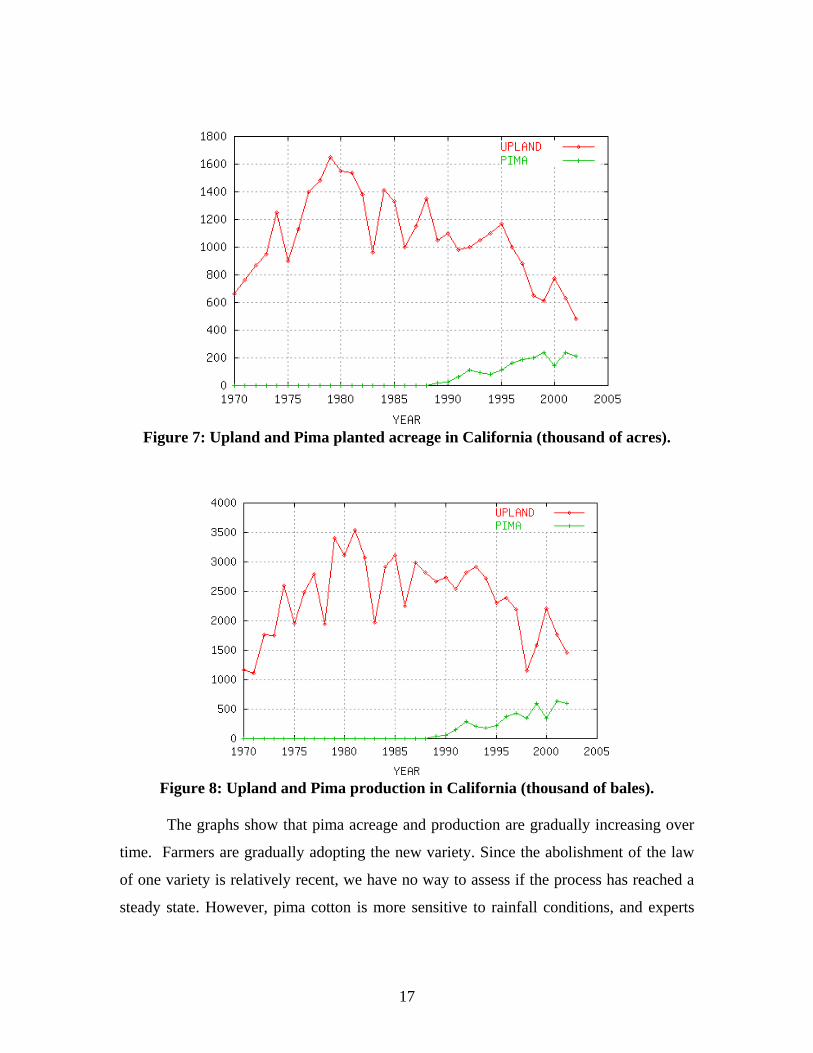
Figure 7: Upland and Pima planted acreage in California (thousand of acres).
Figure 8: Upland and Pima production in California (thousand of bales).
The graphs show that pima acreage and production are gradually increasing over
time. Farmers are gradually adopting the new variety. Since the abolishment of the law
of one variety is relatively recent, we have no way to assess if the process has reached a
steady state. However, pima cotton is more sensitive to rainfall conditions, and experts
17

expect that the final crop pattern in California will be a mixture of pima and upland,
depending on local weather conditions.
The rationale for the adoption of the new variety can be found, in part, in Figure
9, that reports the real grower prices for pima and upland.
Figure 9: Real prices for Pima and Upland (dollars/lb.).
The graph shows that pima growers benefit from a price premium relative to
upland producers. If weather conditions are favorable, pima is considered more
profitable. The time trends also show that the price of upland and pima are cointegrated,
suggesting a strong theoretical argument for modeling aggregate cotton production
regardless of variety (as we did in the previous section).
In this section we adopted a partial adjustment model of the new variety based on
relative prices. Given the relevance of the pima production, the model can provide useful
indications, however it must be pointed out that: (i) the phenomenon is still too recent to
allow reliable statistical analyses based on a time series approach, and (ii) the short time
series poses a strong constraint in the number of explanatory variables that can be
incorporated into the model.
18
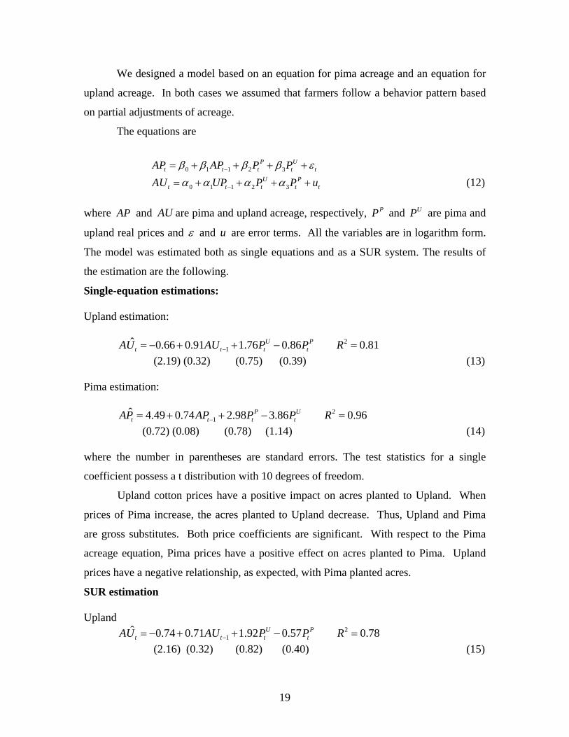
We designed a model based on an equation for pima acreage and an equation for
upland acreage. In both cases we assumed that farmers follow a behavior pattern based
on partial adjustments of acreage.
The equations are
0 1 1 2 3
P Ut t t tAP AP P P tβ β β β−= + + + + ε
t
0 1 1 2 3U P
t t t tAU UP P Pα α α α−= + + + + u (12) where AP and are pima and upland acreage, respectively, AU PP and are pima and
upland real prices and
UP
ε and u are error terms. All the variables are in logarithm form.
The model was estimated both as single equations and as a SUR system. The results of
the estimation are the following.
Single-equation estimations: Upland estimation:
21
ˆ 0.66 0.91 1.76 0.86 0.81U Pt t t tAU AU P P R−= − + + − =
(2.19) (0.32) (0.75) (0.39) (13) Pima estimation:
21
ˆ 4.49 0.74 2.98 3.86 0.96P Ut t t tAP AP P P R−= + + − =
(0.72) (0.08) (0.78) (1.14) (14) where the number in parentheses are standard errors. The test statistics for a single
coefficient possess a t distribution with 10 degrees of freedom.
Upland cotton prices have a positive impact on acres planted to Upland. When
prices of Pima increase, the acres planted to Upland decrease. Thus, Upland and Pima
are gross substitutes. Both price coefficients are significant. With respect to the Pima
acreage equation, Pima prices have a positive effect on acres planted to Pima. Upland
prices have a negative relationship, as expected, with Pima planted acres.
SUR estimation Upland
21
ˆ 0.74 0.71 1.92 0.57 0.78U Pt t t tAU AU P P R−= − + + − =
(2.16) (0.32) (0.82) (0.40) (15)
19

Pima 2
1ˆ 4.42 0.78 2.89 4.26 0.96P Ut t t tAP AP P P R−= + + − =
(1.11) (0.05) (1.00) (1.72) (16) The two procedures (single-equation approach and SUR) give similar estimations. In the
SUR results the coefficient of Pima prices is insignificant in determining Upland acreage.
However, it must be noted that the explanatory variables have a high degree of
multicollinearity.
The model confirms the hypothesis that the relative prices of Upland and Pima are
driving forces in the adoption process at the state level in California.
Conclusions The estimated models indicate that the short-run own-price elasticity of alfalfa
acreage is inelastic (0.35) but more elastic (0.66) when ample water is available. By
applying water marginally through out the growing period, a producer can obtain more
cuttings of alfalfa. Alfalfa yields are also responsive to increases in prices. The own-
price elasticity of yields is 0.08 and highly significant. Alfalfa yields are negatively
related to the previous year’s cotton price. Production is positively related to own price
with an estimated elasticity of 0.44 and significant. Production was negatively related to
risk with an elasticity of risk equal to -0.75. Demand for alfalfa is a derived demand and
is positively related to the number of cows and milk price support and negatively related
to its own price.
The estimated own-price elasticity of cotton acreage is 0.53 and highly
significant. Cotton acreage decreases with an increase in risk in growing cotton and as
price of alfalfa increases. The short-run own-price elasticity of cotton production is
20

0.497 and the long-run estimate is 0.503. The own-price elasticity of cotton demand is -
0.684. Rayon is a substitute for cotton. The empirical results support the fact that alfalfa
and cotton are rotating crops in California.
In recent years there has been an increase in Pima acreage relative to the
traditional Upland variety in California. Upland cotton prices have a positive impact on
acres planted to Upland. When Pima prices increase, the acres planted to Upland
decrease. A similar situation applies to Pima acreage. That is, an increase in Upland
prices causes a decrease in Pima acreage. Thus, the empirical results support that
hypothesis that relative prices of Upland and Pima have a significant impact on the
adoption of the two varieties.
Future research needs to focus on the collection of more data related to the
consumption of California cotton and alfalfa, stocks and inventories, and interstate trade
of alfalfa between California and Oregon and Nevada.
21

References
Davidson, R. and J. MacKinnon. Econometric Theory and Methods, Oxford University
Press, Oxford, 2004.
Evans, J., “Cloud Over Cotton Farmers”, Sacramento Bee, May 3, 2004.
Hamilton, J., Time Series Analysis, Princeton University Press, Princeton, NJ, 1994.
Johnston, W., “Cross Sections of a Diverse Agriculture: Profiles of California’s
Production Regions and Principal Commodities” in California Agriculture Issues
and Challenges, J. Siebert, ed., University of California, Giannini Foundation,
August 1997.
Johnston, W. and A. McCalla, “Whither California Agriculture: Up, Down or Out? Some
Thoughts About the Future”, Giannini Foundation, forthcoming 2004.
Stock, J. and M. Watson. Introduction to Econometrics, Addison-Wesley, Boston, MA,
2003.
White, K., SHAZAM, User’s Reference Manual, Version 9.0, Irwin/McGraw-Hill,
Vancouver, B.C., Canada, 2000.
22
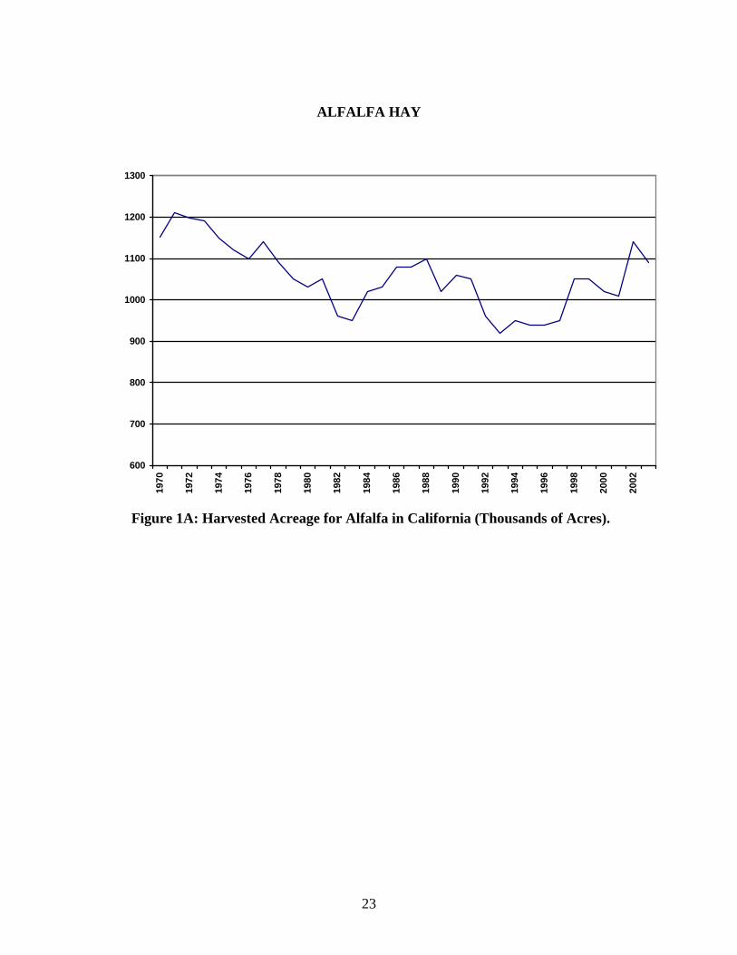
ALFALFA HAY
600
700
800
900
1000
1100
1200
130019
70
1972
1974
1976
1978
1980
1982
1984
1986
1988
1990
1992
1994
1996
1998
2000
2002
Figure 1A: Harvested Acreage for Alfalfa in California (Thousands of Acres).
23

4600
5100
5600
6100
6600
7100
7600
8100
8600
1970
1972
1974
1976
1978
1980
1982
1984
1986
1988
1990
1992
1994
1996
1998
2000
2002
Figure 2A: Alfalfa production in California (Thousands of tons)
5
5,5
6
6,5
7
7,5
1970
1972
1974
1976
1978
1980
1982
1984
1986
1988
1990
1992
1994
1996
1998
2000
2002
Figure 3A: Alfalfa Yield in California (tons)
24

5
25
45
65
85
105
125
145
1970
1972
1974
1976
1978
1980
1982
1984
1986
1988
1990
1992
1994
1996
1998
2000
2002
Figure 4A: Alfalfa Nominal Grower Price in California (12 month average)
25

5
25
45
65
85
105
125
145
Jan1
970
mar
-71
May
1972
Jul1
973
Sep1
974
nov-
75
Jan1
977
mar
-78
May
1979
Jul1
980
Sep1
981
nov-
82
Jan1
984
mar
-85
May
1986
Jul1
987
Sep1
988
nov-
89
Jan1
991
mar
-92
May
1993
Jul1
994
Sep1
995
nov-
96
Jan1
998
mar
-99
May
2000
Jul2
001
Sep2
002
nov-
03
Figure 5A: Alfalfa Nominal Grower Price (Monthly- dollars per ton)
26

5
25
45
65
85
105
125
145
165
1970
1972
1974
1976
1978
1980
1982
1984
1986
1988
1990
1992
1994
1996
1998
2000
2002
Figure 6A: Alfalfa Real Grower Price in California (12 month average, dollars per tons – base 1983/4)
27

5
25
45
65
85
105
125
145
165
185
Jan1
970
feb-
71
mar
-72
apr-
73
May
1974
Jun1
975
Jul1
976
Aug
1977
Sep1
978
Oct
1979
nov-
80
Dec
1981
Jan1
983
feb-
84
mar
-85
apr-
86
May
1987
Jun1
988
Jul1
989
Aug
1990
Sep1
991
Oct
1992
nov-
93
Dec
1994
Jan1
996
feb-
97
mar
-98
apr-
99M
ay20
00
Jun2
001
Jul2
002
Figure 7A: Alfalfa Real Grower Price in California (monthly, dollars per tons– base 1983/4)
28

0
2
4
6
8
10
12
14
16
1970
1972
1974
1976
1978
1980
1982
1984
1986
1988
1990
1992
1994
1996
1998
2000
2002
Figure 8A: Standard Deviation of Monthly Alfalfa Price (Nominal, $/month).
29

0
5
10
15
20
25
30
1970
1972
1974
1976
1978
1980
1982
1984
1986
1988
1990
1992
1994
1996
1998
2000
2002
Figure 9A: Standard Deviation of Monthly Alfalfa Price (Real dollars per month,
base 1983/4).
30

COTTON
400
600
800
1000
1200
1400
1600
180019
70
1972
1974
1976
1978
1980
1982
1984
1986
1988
1990
1992
1994
1996
1998
2000
2002
2004
Figure 10A: Cotton Acreage in California (acres/ in thousands).
31

600
700
800
900
1000
1100
1200
1300
1400
1500
1970
1972
1974
1976
1978
1980
1982
1984
1986
1988
1990
1992
1994
1996
1998
2000
2002
2004
Figure 11A: Cotton Yield in California (pounds).
32

1000
1500
2000
2500
3000
3500
4000
1970
1972
1974
1976
1978
1980
1982
1984
1986
1988
1990
1992
1994
1996
1998
2000
2002
2004
Figure 12A: Cotton Production in California (1000 bales).
33

0
0.1
0.2
0.3
0.4
0.5
0.6
0.7
0.8
0.9
1970
1972
1974
1976
1978
1980
1982
1984
1986
1988
1990
1992
1994
1996
1998
2000
2002
2004
Figure 13A: Nominal Producers’ Price in California for Cotton ($/lb).
34

0
0.2
0.4
0.6
0.8
1
1.2
1.4
1970
1972
1974
1976
1978
1980
1982
1984
1986
1988
1990
1992
1994
1996
1998
2000
2002
Figure 14A: Real Producers’ Price in California for Cotton ($/lb).
35

36

RICE
National vs. State Model
California is one of the major producers of rice in the US. The other most important states are
Arkansas, Louisiana, Mississippi, Missouri and Texas. The market in California appears to be fully
integrated with the southern states, as suggested by an empirical check of the law of one price. This
conclusion is hardly surprising, given that rice is a storable and easily transportable commodity. Figure
1 illustrates the law of one price between California and Arkansas.
Figure 1: Rice grower price (real) in California (RTP) and Arkansas (RPARK)
(in real dollars per cwt.)
A simple ordinary least squares regression of California rice price on Arkansas price gives an
R2 of 0.939 and an estimated slope coefficient between 0.80 and 0.94 (with a 95% confidence level).
Moreover, a simple cointegration test suggests the absence of unit roots in the disturbances. Thus,
California price and Arkansas rice prices move together over the long run. Market integration suggests
1
that a US level model can be useful to describe California rice production. In this study, however, we
present both national and state models.
The US Market
We estimated two models for the US rice industry. The first one is based on a longer time
series, but does not account for policy distortions or trade. The second model considers the influence
of policy and trade but data limitations constrain the length of the available time series.
A simplified model
A simplified production model is
0 1 1 2 2 3 4 1 5ln ln ln lnt t t tQ P P t Q Dt tβ β β β β β− − −= + + + + + +ε (1)
where Q is the quantity of rice production in tons, is rice price per ton , t is a time trend and is a
binary variable identifying the years 1977 and 1983 (outliers).
tP D
Prior to reporting the estimated production function for rice, a brief discussion of some
aberrations of the rice market will be explained. Around 1976-77 there was a price collapse that caused
producers to rotate to other crops or not plant rice at all. This lead to decreases in rice production. In
the early eighties rice prices collapsed again and this caused many growers to forfeit their crop to the
government because the price was below the value of the government loan. This was not only the case
with rice, but other program crops such as wheat and corn. In an attempt to reduce acreage and sell off
the rice that the government had claimed, the government implemented the 50/92 plan. Subsides were
directly linked to production. Thus, if a grower did not produce he was not paid. The 50/92 program
allowed the grower to produce on 50% of his acreage and receive 92% of the subsidies that he would
receive if he had produced on 100% of his land. This reduced production allowed the government to
reduce the stocks of commodities that they had to claim in 1981-82. The 50/92 program ran until about
1988. Since then subsidies have been decoupled from production to prevent problems like this from
happening again. The 50/92 program was popular in the south, especially in Texas where their
2

production was lower and they had low fixed costs of land, but in California it was only widely used
for a few years. Policy variables are incorporated into some of the models below.
The estimated partial adjustment production model for rice, for the time period 1972-2004, is:
1 2 1ˆln 2.32 0.23ln 0.07 ln 0.02 0.41ln 0.26
(0.68) (0.07) (0.08) (0.00) (0.16) (0.07)t t t tQ P P t Q− − −= + − + + − tD (2)
with R2 = 0.896 and n = 33. The Durbin h test did not indicate problems with autocorrelation. The
coefficient on lagged production is positive and significant. This indicates that there is some
adjustment each year in the production of rice. By removing the lags, i.e., by assuming 1t tQ Q −= , the
long-run price elasticity of production is 0.27 which is inelastic and significant, but indicates that rice
producers do respond to price changes. The estimated coefficient on the time trend variable is 0.02 and
significant indicating a positive trend over time. The estimated coefficient on the dummy variable is
negative (coefficient = -0.26) and significant for the outlier years as expected.
Figure 2 describes the fit of the regression (in logarithmic scale--the original series is in 000 cwt).
Figure 2: US rice production actual (LRR) and estimated (RHAT)
(logarithmic scale)
3
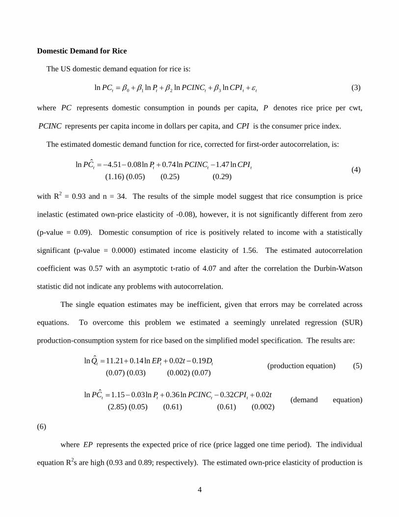
Domestic Demand for Rice
The US domestic demand equation for rice is:
0 1 2 3ln ln ln lnt t tPC P PCINC CPIt tβ β β β= + + + +ε
t
tD
(3)
where represents domestic consumption in pounds per capita, denotes rice price per cwt,
represents per capita income in dollars per capita, and is the consumer price index.
PC P
PCINC CPI
The estimated domestic demand function for rice, corrected for first-order autocorrelation, is:
(4) ˆln 4.51 0.08ln 0.74ln 1.47 ln
(1.16) (0.05) (0.25) (0.29) t t tPC P PCINC CPI= − − + −
with R2 = 0.93 and n = 34. The results of the simple model suggest that rice consumption is price
inelastic (estimated own-price elasticity of -0.08), however, it is not significantly different from zero
(p-value = 0.09). Domestic consumption of rice is positively related to income with a statistically
significant (p-value = 0.0000) estimated income elasticity of 1.56. The estimated autocorrelation
coefficient was 0.57 with an asymptotic t-ratio of 4.07 and after the correlation the Durbin-Watson
statistic did not indicate any problems with autocorrelation.
The single equation estimates may be inefficient, given that errors may be correlated across
equations. To overcome this problem we estimated a seemingly unrelated regression (SUR)
production-consumption system for rice based on the simplified model specification. The results are:
(production equation) (5) ˆln 11.21 0.14ln 0.02 0.19
(0.07) (0.03) (0.002) (0.07)t tQ EP t= + + −
(demand equation)
(6)
ˆln 1.15 0.03ln 0.36ln 0.32 0.02 (2.85) (0.05) (0.61) (0.61) (0.002)
t t t tPC P PCINC CPI t= − + − +
where EP represents the expected price of rice (price lagged one time period). The individual
equation R2s are high (0.93 and 0.89; respectively). The estimated own-price elasticity of production is
4

0.14 and but not significant. The own-price elasticity of demand for rice is -0.03, but it is not
significant either. The income elasticity of demand for domestic rice is 0.36 and is also not significant.
The explanatory variables were highly collinear which accounts for some of the estimated coefficients
being insignificant.
An Alternative Model
An alternative model considers policy and exports. However, due to the short time series
(1986-2003), the model must be parsimonious. For a comprehensive and disaggregated treatment of
the influence of commodity programs on the rice acreage response to market prices, see McDonald and
Sumner.1
The least squares estimated production equation is:
(7) 1ˆln 10.843 0.176ln 0.003 0.034
(0.236)(0.067) (0.001) (0.033)t t tQ P PSE−= + + + t
with R2 = 0.87 and n = 18. The policy variable, , is the OECD percentage producer support
estimate for the U.S. that is a comprehensive or aggregate measure of total policy support. The other
explanatory variables are as defined above. The estimated policy coefficient is positive with a value of
0.003 and almost significant (p-value = 0.079). The estimated expected price elasticity of production is
0.176 and is significant (p-value = 0.02). The estimated coefficient on the time trend indicates that
production has been increasing over time.
tPSE
Overall the results suggest that public support has a significant and positive effect on
production. The fit of the regression is depicted in Figure 3.
1 McDonald and Sumner incorporate detailed rice commodity programs into their approach. Their approach is based on an econometric estimation of a marginal cost curve, some assumptions about the distribution of parameters of their cost function combined with a simulation methodology. Their main policy results indicate that models that do not take into account all the programs’ rules produce smaller structural parameters. They cite previous studies that find the acreage elasticites for rice vary from 0.09 to 0.34 which their results indicate are too small.
5

Figure 3: US rice production actual (LTR) and estimated (RHAT)
(in billions of lbs)
Export Demand for Rice
The estimated export equation for rice is:
(8) , , ,ˆln 31.81 0.49ln 0.91ln 1.99ln 0.04
(6.52)(0.19) (0.31) (0.62) (0.01)t us t Thai t Japan tEX P P Inc t= − + − +
with R2 = 0.78, n = 18, and where represents US exports of rice in 000 cwt, represents the
grower price for US rice in $/cwt, denotes the price for rice in Thailand (the major competitor in
the world market) and
tEX USP
ThaiP
JapanInc represents per capita income in Japan (the major importer of US rice).
The estimated results indicate that US exports decrease with US price increases (US price elasticity of
exports is -0.49), increase with increases in Thailand rice prices, and have been increasing over time,
conditioned on the other variables. The negative sign on per capita income in Japan was not expected.
6

Figure 4: US rice export actual (LEX) and estimated (EHAT)
In order to account for price endogeneity, correlated errors across equations, and to obtain more
efficient estimates, we estimated a system of two equations for US rice, under the market clearing
assumption. Lagged price was used as the instrumental variable for current price to account for
endogeneity of prices. The system was estimated by iterative three stage least squares (3SLS). The
estimators have the same asymptotic properties as maximum likelihood estimators. That is, they are
consistent, asymptotically normally distributed and efficient. Iterative 3SLS converge to the same
value as MLE, but are not equivalent because of a Jacobian term in the likelihood function. The first
equation is a production function and the second equation is a demand function. The system results
are:
, ,ˆln 8.92 0.45ln 0.27 ln 0.01 0.06
(1.74) (0.39) (0.14) (0.01) (0.02)t US t Thai t tQ P P PSE= + + + + t
,nc
(9)
, ,ˆln 2.68 0.36 ln 0.39 ln 0.33 0.34
(3.77) (0.17) (0.25) (0.21) (0.49)t US t Thai t t Japan tQ P P Inc I= − + + +
(10)
7

The fit of the system is depicted graphically in Figure 5 (the R2 for the first equation is 0.718
and for the second is 0.888).
Figure 5: Estimation of supply and demand for US rice, under market equilibrium assumption
The estimated US price expectation (the lag price) elasticity of supply is 0.45 which is also
inelastic but is not significant. The estimated coefficient of Thailand price of rice is 0.27 with a t-ratio
of about two. The index for price support is positive but not significant. There is also a positive (0.06)
and significant time trend in the supply of rice. According to the estimated price coefficient (-0.36), the
elasticity of demand of US rice implies that an increase of 1% in price results in a decrease of 0.36%
change in the quantity demanded. As the price of Thailand rice increases, the demand for US rice
increases, but again the estimated coefficient is not significant. The income elasticity is 0.33 and the
estimated coefficient of Japanese income is 0.34 as expected. Both coefficients are not significant,
however.
8

California Market
The estimated production function of California rice is:
1ˆln 7.56 0.48ln 0.11 0.005 0.04 1.21 1.23 *
(0.72) (0.16) (0.05) (0.04) (0.01) (0.52) (0.48)t t t t tQ P Pay Loan t D D Pay−= + + − + + − t t (11)
with R2 = 0.816, n = 21, and where denotes California production, denotes grower price,
represents direct payments, are the interest rate on marketing loans and is a dummy variable
identifying the years 1996 and after to account for policy changes.
Q P Pay
Loans D
The estimated own-price elasticity is 0.48 (and significant) which is higher than the corresponding
estimated value for US production. Producers respond positively to increases in direct payments and to
policy changes occurring after 1996. There is also a positive time trend. Interest rates on marketing
loans did not have a significant impact on California production. Figure 6 depicts the fit of the
California production model.
Figure 6: California rice production actual (LRR) and estimated (RRHAT)
9

Conclusions
Rice producers in California and throughout the United States respond positively to increases in rice
prices. The short-run price elasticity of production, based on a partial adjustment model, for the US
was estimated to be 0.23. When policy variables were included in the production equation the price
elasticity dropped to 0.18 (see eq. 7). Rice producers respond positively to support programs. The
production equation was an aggregated one. For a disaggregated approach that estimates how rice
producers respond to different support programs, see McDonald and Sumner.
The estimated own-price elasticity of demand for rice was found to be inelastic (-0.140) for a SUR
system. The income elasticity for rice was estimated to be 0.74 in a single-equation demand function
(eq. 4).
US rice producers export less when the US price increases (estimated elasticity =-0.49). They
export more when the Thailand rice price increases (estimated Thailand price elasticity of 0.91) since
Thailand is a major competitor in the world market.
10

References
McDonald, J. and D. Sumner, “The Influence of Commodity Programs on Acreage Response to Market
Price: with an Illustration Concerning Rice Policy in the United States”, American Journal of
Agricultural Economics, 85(4): 2003: 857-871.
11
TOMATOES
Background
The United States is the world's second leading producer of tomatoes, after China. Fresh and
processed tomatoes combined accounted for almost $2 billion in cash receipts during the early 2000s.
Mexico and Canada are important suppliers of fresh market tomatoes to the United States and Canada
is the leading importer of U.S. fresh and processed tomatoes.
The characteristics of tomato consumption are changing. Fresh tomatoes consumption
increased by 15% between the early ‘90s and early 2000s, while the use of processed products declined
9%. Currently, the per capita consumption is 18 pounds per person of fresh tomatoes, and 68 pounds
for processed tomatoes (fresh-weight basis).
The U.S. fresh and processing tomato industries consist of separate markets. According to ERS
(website) four basic characteristics distinguish the two industries. Tomato varieties are bred
specifically to serve the requirements of either the fresh or the processing markets. Processing requires
varieties that contain a higher percentage of soluble solids (averaging 5-9 percent) to efficiently make
tomato paste, for example.
• Most tomatoes grown for processing are produced under contract between growers and
processing firms. Fresh tomatoes are largely produced and sold on the open market.
• Processing tomatoes are machine-harvested while all fresh-market tomatoes are hand-picked.
• Fresh-market tomato prices are higher and more variable than processing tomatoes due to larger
production costs and greater market uncertainty
Policy
Tomato production is not covered by price or income support. However, tomato producers may
benefit from general, non crop specific-programs such as federal crop insurance, disaster assistance,

2
and western irrigation subsidies. The only federal marketing order in force for tomatoes covers the
majority of fresh-market tomatoes produced in Florida between October and June.
With respect to imports, the United Stated negotiated a voluntary price restraint on fresh tomato
imports from Mexico starting in 1996. Mexico agreed to set a floor price of $0.21 per pound of
tomatoes exported to the United States The effect of the policy was to reduce Mexican exports to the
U.S. and there were sizeable fresh tomato diversions (to other importing countries) and diversions into
processing; see Baylis and Perloff for more details of this policy.
California Production
California is the second leading producer of fresh tomatoes in the US, after Florida. Figures 1-3
compares fresh tomatoes planted acreage, production and nominal price for US, Florida and California.
California accounts for about 95 percent of the area harvested for processing tomatoes in the
United States—up from 79 percent in 1980 and 87 percent in 1990. The other major producers are
Texas, Utah, Illinois, Virginia, and Delaware and Florida. In Figure 1, total U.S. fresh tomato acreage
has declined over the period 1960 to 2002, but acreage in California and Florida has remained steady.
The declined in acreage has come from the states of Texas, Utah, Illinois, Virginia, and Delaware
(Lucier). Figures 4-6 illustrates the trends for California and US planted acreage, production and
nominal prices for processed tomatoes.

3
0
20,000
40,000
60,000
80,000
100,000
120,000
140,000
160,000
180,000
200,000
1960
1963
1966
1969
1972
1975
1978
1981
1984
1987
1990
1993
1996
1999
2002
years
Acres
US
CA
FL
Figure 1: Fresh tomato acreage 1960-2002 – (source ERS)
0
5,000
10,000
15,000
20,000
25,000
30,000
35,000
40,000
45,000
196019631966196919721975197819811984198719901993199619992002
years
CWT
US
CA
FL
Figure 2: Fresh tomato production 1960-2002 – (source ERS)

4
0
5
10
15
20
25
30
35
40
45
1960
1963
1966
1969
1972
1975
1978
1981
1984
1987
1990
1993
1996
1999
2002
years
$/CWT
US
CA
FL
Figure 3a: Fresh tomato nominal prices 1960-2002 –(source ERS)
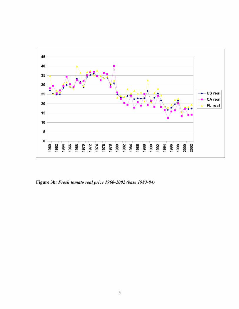
5
0
5
10
15
20
25
30
35
40
45
1960
1962
1964
1966
1968
1970
1972
1974
1976
1978
1980
1982
1984
1986
1988
1990
1992
1994
1996
1998
2000
2002
US real
CA real
FL real
Figure 3b: Fresh tomato real price 1960-2002 (base 1983-84)

6
0
50,000
100,000
150,000
200,000
250,000
300,000
350,000
400,000
450,000
196019631966196919721975197819811984198719901993199619992002
years
Acres US
CA
Figure 4: Processing tomato acreage 1960-2002 – (source ERS)
0
2,000,000
4,000,000
6,000,000
8,000,000
10,000,000
12,000,000
14,000,000
1960
1963
1966
1969
1972
1975
1978
1981
1984
1987
1990
1993
1996
1999
2002
years
Sh
ort
to
ns
US
CA
Figure 5: Processing tomato production 1960-2002 – (source ERS)

7
0
10
20
30
40
50
60
70
80
1960
1963
1966
1969
1972
1975
1978
1981
1984
1987
1990
1993
1996
1999
2002
years
Sh
ort
to
ns
US
CA
Figure 6: Processing tomato nominal prices 1960-2002 ($/ton) – (source ERS)
Processing Tomatoes
Tomato growing is based on grower-processor contract agreements. The majority of production
is traded this way with the spot market playing a marginal role. Most initial processing is by firms that
manufacture tomato paste, a raw ingredient. Tomato paste is storable up to 18 months. Downstream
firms transform the paste in final consumer products. According to the Food Institute, at the end of the
process, raw material (tomatoes and fees) account for 39%-45% of total production cost.
According to the ERS, there was a radical structural change in the processing industry in the
late 1980’s and early 1990’s. A period of relatively high prices in the late 1980s triggered new
investments. This finally resulted in excess supply and decreasing prices. As a consequence, many
processors went bankrupt and the whole industry was restructured. The current structure is the result of
such adjustments.

8
Estimation
A brief industry description highlights two key points prior to the estimations.
Price expectations. The majority of production is sold under contract. This has two implications: i)
producers know (with good approximation) prices when planning production, so we do not need to
model expectations; rather we assume perfect information, ii) the actual contract price is unobservable,
being industry private information. It is reasonable to assume that the spot market price is correlated
with contract price according to the additive error formula:
spot price = contract price + error .
We use the spot price as a proxy for the real contract price. However, since the measurement error is
likely to be correlated with the error terms in the production equations (for example in case of
unexpected shortage, we expect higher spot prices) we use an instrumental variable (IV) approach. The
instrument is the previous year’s spot price, which is correlated with the current spot price, but
uncorrelated with random shocks in current production.
Structural change. The industry underwent structural changes from the late ‘80s until the early ‘90s.
Much of the change is likely due to continued expansion in food-service demand, especially for pizza,
taco, and other Italian and Mexican foods (Lucier). Increased immigration and changes in America’s
tastes and preferences have contributed to rising per capita tomato use (Lucier, et al). Commercial
varieties were developed to expedite packing, shipping, and retailing in the processing market.
Mechanical harvesting and bulk handling systems replaced hand harvest of processing tomatoes in the
California in the 1960’s as the new varieties were introduced. Increases in yields are due to the
development of higher yielding hybrid varieties and improved cultural practices such as increases in
use of transplanting (Plummer). The hypothesis of structural change was tested on both the supply and
demand side.
Acreage

9
The acreage equation is based on a partial adjustment model:
0 1 2 1 3ln ln ln
t t t tA P A t! ! ! ! "#= + + + + (1)
where tA represents acreage at time t in actual acres,
tP represents the spot price of processing tomatoes
in $/cwt, and t is a time trend.
The OLS estimated acreage function for the years 1960-2002 is:
1ˆln 5.67 0.47 ln 0.32ln 0.03
(1.38) (0.12) (0.13) (0.01)
t t tA P A t
!= + + + (2)
with R2 = 0.815, n = 42 and where the numbers in parentheses are standard errors.
The instrumental variable estimated acreage equation is:
1ˆln 5.67 0.41ln 0.36ln 0.02
(1.39) (0.18) (0.14) (0.01)
t t tA P A t
!= + + + (3)
with R2 = 0.814 and n = 42.
Figures 7 and 8 compare the fits of the two regressions.

10
Figure 7: OLS estimation of processing tomato acreage (in acres).
Figure 8: IV estimation of processing tomato acreage (in acres).
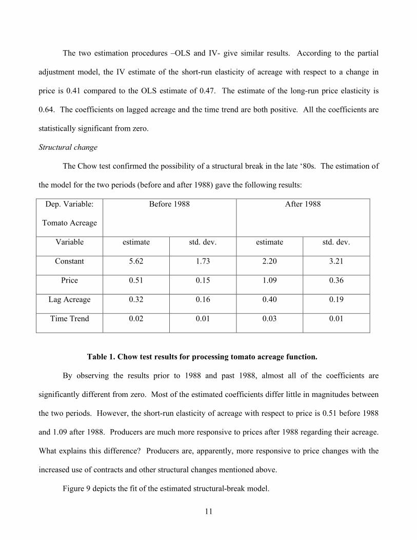
11
The two estimation procedures –OLS and IV- give similar results. According to the partial
adjustment model, the IV estimate of the short-run elasticity of acreage with respect to a change in
price is 0.41 compared to the OLS estimate of 0.47. The estimate of the long-run price elasticity is
0.64. The coefficients on lagged acreage and the time trend are both positive. All the coefficients are
statistically significant from zero.
Structural change
The Chow test confirmed the possibility of a structural break in the late ‘80s. The estimation of
the model for the two periods (before and after 1988) gave the following results:
Dep. Variable:
Tomato Acreage
Before 1988 After 1988
Variable estimate std. dev. estimate std. dev.
Constant 5.62 1.73 2.20 3.21
Price 0.51 0.15 1.09 0.36
Lag Acreage 0.32 0.16 0.40 0.19
Time Trend 0.02 0.01 0.03 0.01
Table 1. Chow test results for processing tomato acreage function.
By observing the results prior to 1988 and past 1988, almost all of the coefficients are
significantly different from zero. Most of the estimated coefficients differ little in magnitudes between
the two periods. However, the short-run elasticity of acreage with respect to price is 0.51 before 1988
and 1.09 after 1988. Producers are much more responsive to prices after 1988 regarding their acreage.
What explains this difference? Producers are, apparently, more responsive to price changes with the
increased use of contracts and other structural changes mentioned above.
Figure 9 depicts the fit of the estimated structural-break model.

12
Figure 9: Structural break model for processing tomato acreage (in acres)
Production
The partial adjustment model for processed tomato production is
0 1 2 1 3
ln ln lnt t t tQ P Q t! ! ! ! "#= + + + + (4)
where tQ denotes production at time t in tons,
tP represents real price of processing tomatoes in $/cwt,
and t is a time trend. The OLS estimated production function is
1ˆln 11.00 0.45ln 0.10ln 0.04
(1.98) (0.13) (0.14) (0.01)
t t tQ P Q t
!= + + + (5)
with R2 = 0.92 and n = 42.
The same model, estimated by using lagged prices as instrumental variables, gave comparable
results:
1ˆln 11.03 0.55ln 0.07 ln 0.05
(1.99) (0.19) (0.15) (0.01)
t t tQ P Q t
!= + + + (6)

13
with R2 = 0.91 and n = 42. The OLS estimate of the own-price elasticity is 0.45 compared to that of
0.55 for the instrumental variables estimate. Both coefficients are significant. Coefficients of lagged
acreage are both positive but not significant. And both coefficients on the time trends are positive and
significant.
Figures 10 and 11 compare the fit of the two estimations.
Figure 10: Production estimation for processing tomato (OLS) in tons.
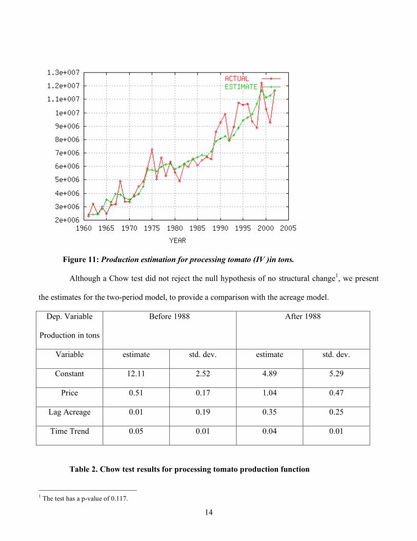
14
Figure 11: Production estimation for processing tomato (IV )in tons.
Although a Chow test did not reject the null hypothesis of no structural change1, we present
the estimates for the two-period model, to provide a comparison with the acreage model.
Dep. Variable
Production in tons
Before 1988 After 1988
Variable estimate std. dev. estimate std. dev.
Constant 12.11 2.52 4.89 5.29
Price 0.51 0.17 1.04 0.47
Lag Acreage 0.01 0.19 0.35 0.25
Time Trend 0.05 0.01 0.04 0.01
Table 2. Chow test results for processing tomato production function
1 The test has a p-value of 0.117.

15
With respect to the production model, the two-period approach suggests that production after 1988
became more elastic. An estimated price elasticity of 0.51 before 1988 versus an estimate of 1.04 after
1988. Both coefficients are significant. Figure 12 illustrates the fit of the estimation.
Figure 12: Structural break model for processing tomato production in tons.
Demand
In this section two demand models for processing tomatoes are presented. The first one
describes the demand for processing tomatoes at the farm level and the second one illustrates the final
demand (at the consumer level) for tomato products.
Demand for processing tomatoes
The demand for processing tomatoes is a function of farmer prices and the price index for
tomato paste. The data refer to 21 time periods (from 1982 to 2002). The model describes the industry
demand under the assumptions of price taking behavior and market equilibrium. Industry expectations

16
are modeled using lagged prices. The regression model has been estimated with a moving average
process of order one. The derived demand equation for processed tomatoes is:
0 1 1 2 1 3
ln lnt t tQ PF PR t! ! ! !" "= + + + (7)
where tQ represents the quantity demanded of California processing tomatoes ,
1tPF
!denotes the
grower price, lagged one time period, 1t
PR!
is the price of tomato paste, lagged one time period, and t
is a time trend.
The estimated demand equation is
1 1ˆln 15.67 0.18ln 0.16ln 0.03
(0.06) (0.05) (0.04) (0.02)
t t tQ PF PR t
! != ! + + (8)
where R2 = 0.815 and n = 21. Based on the estimates, the demand for California processing tomatoes
is inelastic (a statistically significant own-price estimated elasticity of -0.18). The coefficient of tomato
paste price is 0.16 and significant. As the price of tomato paste increases the demand for processing
tomatoes increases. This is as expected since the demand for processing tomatoes is a derived demand.
Figure 13 shows the fit of the regression.
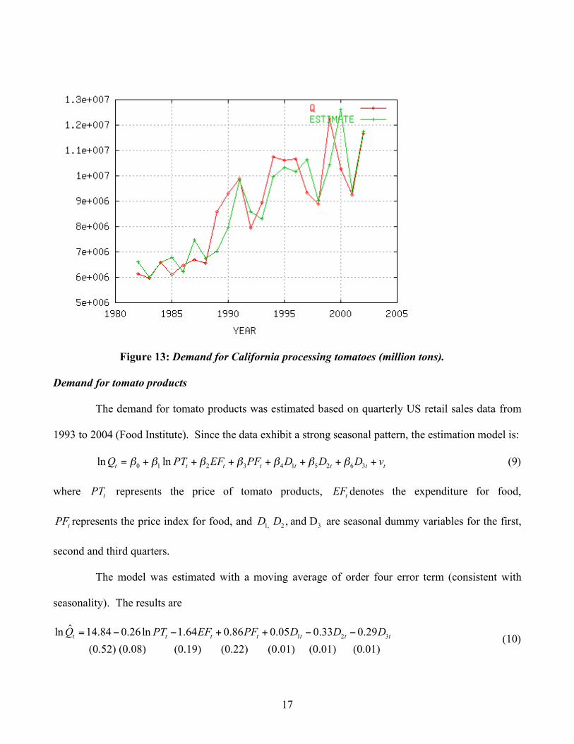
17
Figure 13: Demand for California processing tomatoes (million tons).
Demand for tomato products
The demand for tomato products was estimated based on quarterly US retail sales data from
1993 to 2004 (Food Institute). Since the data exhibit a strong seasonal pattern, the estimation model is:
0 1 2 3 4 1 5 2 6 3
ln lnt t t t t t t tQ PT EF PF D D D v! ! ! ! ! ! != + + + + + + + (9)
where t
PT represents the price of tomato products, t
EF denotes the expenditure for food,
tPF represents the price index for food, and
1, 2 3, and DD D are seasonal dummy variables for the first,
second and third quarters.
The model was estimated with a moving average of order four error term (consistent with
seasonality). The results are
1 2 3ˆln 14.84 0.26ln 1.64 0.86 0.05 0.33 0.29
(0.52) (0.08) (0.19) (0.22) (0.01) (0.01) (0.01)
t t t t t t tQ PT EF PF D D D= ! ! + + ! ! (10)

18
where R2 = 0.99 n = 48. The demand for tomato products is inelastic (a significant own-price elasticity
estimate of -0.26) and on average is higher during the first and the fourth quarters (since fresh tomatoes
are less available). The sign of the food expenditure elasticity is negative which is not as expected.
Figure 14 illustrates the fit of the regression.
Figure 14: Consumers’ demand for processing tomato products (1st quarter 1993-4th quarter 2004)

19
Fresh Tomatoes
Per capita consumption of fresh tomatoes has been increasing since the ‘80s (Figure 15).
Higher demand triggered a structural adjustment in the industry. Figure 1 shows that, initially, the
main acreage adjustment was in Florida, while California increased acreage sharply in the late ‘80s.
0
2
4
6
8
10
12
14
16
18
20
1970
1972
1974
1976
1978
1980
1982
1984
1986
1988
1990
1992
1994
1996
1998
2000
2002
po
un
ds
pe
r c
ap
ita
Figure 15: US per capita consumption of fresh tomatoes
Given this trend in the industry the estimations allowed for a structural break. The two
periods are 1960-1987 and 1988-2002.
Acreage for Fresh Tomatoes
The acreage model was estimated assuming a partial adjustment process. Price expectations
have been modeled using the previous year’s price for the period 1960-1987 and a two-year lagged
price before the period 1988-2002. This was done because after the structural change, the prices
exhibits an alternate pattern, so that the current price is negatively correlated with the previous year, but

20
positively correlated with two periods before. Finally we tested the influence of the processing
industry on the fresh tomato acreage, by using the price of processing tomato as a regressor.
What accounts for the structural break in 1987 in fresh tomato acreage? Much of the increase
in California acreage can be explained as a response to changes in consumption patterns, according to
the USDA. In terms of consumption, tomatoes are the Nation's fourth most popular fresh-market
vegetable behind potatoes, lettuce, and onions. Fresh-market tomato consumption has been on the rise
due to the enduring popularity of salads, salad bars, and sandwiches such as the BLT (bacon-lettuce-
tomato) and subs. Perhaps of greater importance has been the introduction of improved tomato
varieties, consumer interest in a wider range of tomatoes (such as hothouse and grape tomatoes), a
surge of immigrants with vegetable-intensive diets, and expanding national emphasis on health and
nutrition. After remaining flat during the 1960s and 1970s at 12.2 pounds, fresh use increased 19
percent during the 1980s, 13 percent during the 1990s, and has continued to trend higher in the current
decade. Although Americans consume three-fourths of their tomatoes in processed form (sauces,
catsup, juice), fresh-market use exceeded 5 billion pounds for the first time in 2002 when per capita use
also reached a new high at 18.3 pounds. Because of the expansion of the domestic
greenhouse/hydroponic tomato industry since the mid-1990s, it is likely per capita use is at least 1
pound higher than currently reported by USDA (the Department does not currently enumerate domestic
greenhouse vegetable production). One medium, fresh tomato (about 5.2 ounces) has 35 calories and
provides 40 percent of the U.S. Recommended Daily Amount of vitamin C and 20 percent of the
vitamin A. University research shows that tomatoes may protect against some cancers.
he partial adjustment acreage function for fresh tomatoes is:
0 1 2 3 4 1
ln ln ln lnt t t t tA EP PP t A! ! ! ! ! "#= + + + + + (11)
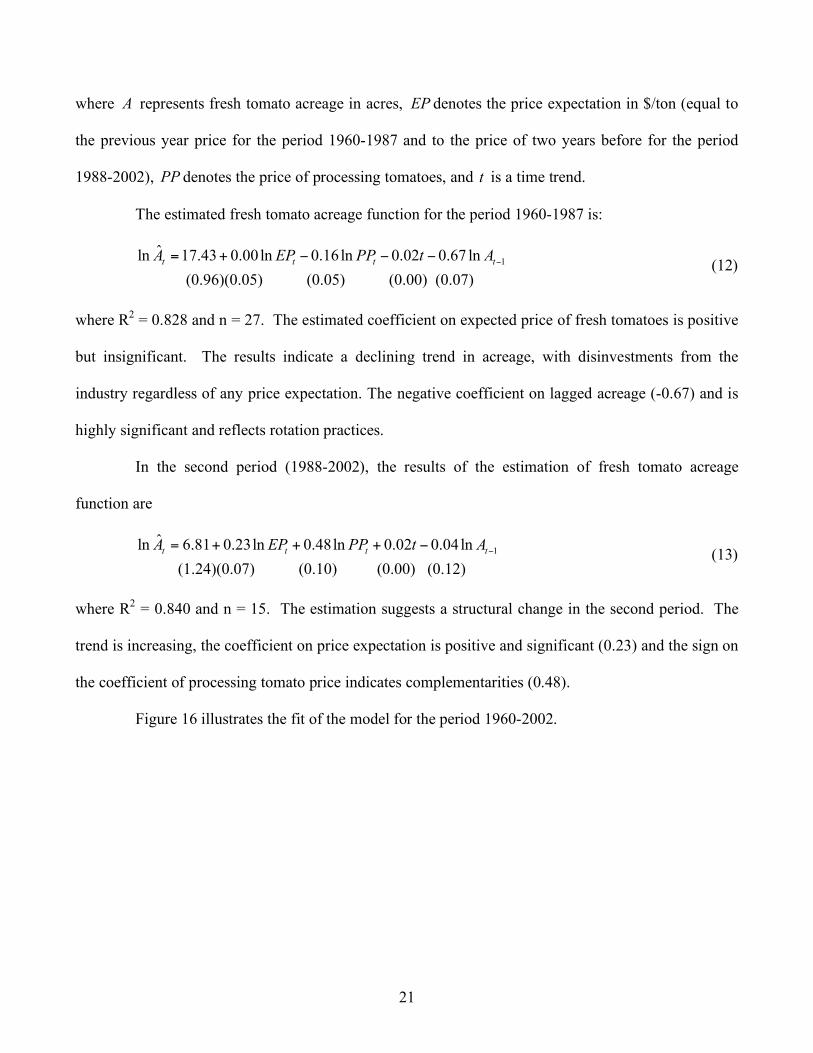
21
where A represents fresh tomato acreage in acres, EP denotes the price expectation in $/ton (equal to
the previous year price for the period 1960-1987 and to the price of two years before for the period
1988-2002), PP denotes the price of processing tomatoes, and t is a time trend.
The estimated fresh tomato acreage function for the period 1960-1987 is:
1ˆln 17.43 0.00ln 0.16ln 0.02 0.67 ln
(0.96)(0.05) (0.05) (0.00) (0.07)
t t t tA EP PP t A
!= + ! ! ! (12)
where R2 = 0.828 and n = 27. The estimated coefficient on expected price of fresh tomatoes is positive
but insignificant. The results indicate a declining trend in acreage, with disinvestments from the
industry regardless of any price expectation. The negative coefficient on lagged acreage (-0.67) and is
highly significant and reflects rotation practices.
In the second period (1988-2002), the results of the estimation of fresh tomato acreage
function are
1ˆln 6.81 0.23ln 0.48ln 0.02 0.04ln
(1.24)(0.07) (0.10) (0.00) (0.12)
t t t tA EP PP t A
!= + + + ! (13)
where R2 = 0.840 and n = 15. The estimation suggests a structural change in the second period. The
trend is increasing, the coefficient on price expectation is positive and significant (0.23) and the sign on
the coefficient of processing tomato price indicates complementarities (0.48).
Figure 16 illustrates the fit of the model for the period 1960-2002.

22
Figure 16: California fresh tomato acreage (in acres).
Production
The partial adjustment model for fresh tomato production is:
2
0 1 2 3 4 5 6 1 ,79ln ln ln ln
t t t t t t tQ EP PP t t W Q D! ! ! ! ! ! ! "#= + + + + + + + + (14)
where Q represents annual production in tons, EP denotes the price expectation in $/ton, PP denotes
the price of processing tomatoes2, also in $/ton, t is a time trend, t
W represents the water availability
(measured by the four river index) and D is a dummy variable identifying the year 1979 which had an
exceptional yield. Note that in this equation the time trend including the quadratic trend, captures the
effects of technological change. The model was estimated separately for the two time periods,
assuming a moving average error process which is consistent with a partial adjustment specification.
The results are as follows:
2 For production, slightly better results can be obtained by using cotton as a competing crop. However, since cotton performs poorly in explaining acreage, we kept processing tomatoes in the estimation for consistency with the acreage equation.

23
Period 1960-1987:
2
1 ,79ˆln 10.04 0.22ln 0.04 0.01 0.00 0.00 0.11ln 0.37
(1.51)(0.12) (0.04) (0.01) (0.00) (0.00) (0.14) (0.07)
t t t t t tQ EP PP t t W Q D
!= + ! ! + + + +
(15)
where R2 = 0.932 and n = 27.
Period 1988-2002:
2
1ˆln 6.82 0.27 ln 0.05 0.02 0.00 0.00 0.33ln
(5.21) (0.11) (0.31) (0.09) (0.00) (0.01) (0.47)
t t t t tQ EP PP t t W Q
!= + ! ! + + +
(16)
where R2 = 0.789 and n = 15. Based on the estimations, the short run elasticity of fresh tomato
production with respect to price expectations was 0.22 before 1987 and 0.27 after 1987. There is no
statistical evidence of change in the values of elasticities after the structural break. Given the partial
adjustment model, the estimation of long run elasticity is 0.247 (before 1988) and 0.403 (from 1988
on). The trend term coefficients were not significant nor were the coefficienets on the lagged
production terms. Figure 17 describes the fit of the regression.

24
Figure 17: California fresh tomato production (in tons).
Demand
The US demand for fresh tomatoes has been modeled using the Almost Ideal Demand
System. The system estimates simultaneously the demand for four of the major vegetables: tomatoes,
lettuce, carrots and cabbage. The approach assumes that consumers are price takers and that consumers
of the four goods have preferences that are weakly separable. The assumption of weak separability
permits the demand for a commodity to be written as a function of its own price, the price of substitutes
and complements, and group expenditure.
The almost ideal demand system is
ln ln( )iit i ij j i it
j t
xw p
P! " # $
%= + + +& (17)

25
where iw represents the ith budget share of commodity i,
jp denotes the jth price of the jth good,
tx is
group expenditure for the particular set of commodities (fresh tomatoes, carrots, lettuce, and cabbage),
and tP! is a translog deflator and is given by
0ln ln (1/ 2) ln lnt k k ij i j
k i j
P p p p! ! "#= + +$ $$ .
Adding-up restrictions require that 1,i
! =" 0,ij
i
! =" and 0.i
i
! =" Homogeneity
requires 0,ij
j
! =" and symmetry requiresij ji! != . These conditions hold globally, that is, at every
data point.
The demand functions for tomatoes, lettuce and carrots were estimated by maximum
likelihood estimation methods, and the results were recovered for the cabbage equation from adding up.
The estimated elasticities of demand with respect to prices and income have been calculated from the
regression coefficients. The income elasticity is given by
1 /i i i
w! "= +
and the price elasticities are given by
[ ( ln )] /ij ij ij i j ik k i
k
p w! " # $ % #= & + & +'
where 1ij! = if i j= , zero otherwise.
. The data are for the time period, 1981-2004 and prices are retail prices. The almost ideal
demand system was estimated with a first-order autoregressive process ( ˆ 0.77! = with an associated
asymptotic standard error of 0.08). The estimated elasticities for the fresh vegetable subsystem are
given in Table 1.

26
Table 1: Estimated elasticities calculated using the AIDS estimation. Estimated AIDS Elasticities Tomato Carrots Lettuce Cabbage
Tomato -0.32*** (0.10)
-0.03 (0.09)
-0.07 (0.05)
-0.002 (0.02)
Carrots -1.51* (0.78)
-0.53* (0.21)
-0.48 (0.37)
-0.33 (0.45)
Lettuce -0.19*** (0.05)
-0.09 (0.13)
-0.71*** (0.20)
-0.16 (0.72)
Cabbage -0.01 (0.04)
-0.17 (0.25)
-0.98 (0.88)
0.12 (0.55)
Income 0.89*** (0.14)
1.44*** (0.24)
0.96*** (0.30)
1.06** (0.41)
a) ***: Significant at the .01 level. **Significant at the .05 level. *Significant at the .10 level. b) Reported standard errors are bootstrap standard errors computed using a subroutine in SAS written by Dr. Barry Goodwin.
The own price elasticity of tomatoes is estimated to be -0.32, which is highly statistically
significant. Therefore demand for fresh tomatoes is relatively inelastic with respect to changes in retail
prices. The own-price elasticity of carrots is -0.53 and for lettuce it is -0.71. The estimate of the own-
price elasticity of cabbage is positive at 0.12, which is counterintuitive. This finding, however, is not
statistically significant. The estimated second-stage expenditure elasticities are all positive and range in
values from 0.89 to 1.44. In all cases the expenditure elasticities are statistically significant. All of the
cross prices elasticities are negative indicating that the four fresh vegetables are complements. Only the
complementarities between tomato quantity with carrot and lettuce prices are statistically significant.
Conclusions
Models for both fresh and processed tomatoes were developed and estimated. An almost ideal demand
subsystem was estimated for four fresh vegetables that included tomatoes, carrots, lettuce, and cabbage.
The second-stage own-price elasticities were all inelastic except for cabbage which was unexpectedly
positive. The conditional expenditure or income elasticites varied from 0.89 for fresh tomatoes to 1.44
for carrots. All of the cross-price elasticities were negative indicating that the four fresh vegetables are

27
gross complements. A plausible explanation for this is that the four commodities are used in salads,
especially given that no significant complementarities were found with respect to fresh cabbage.
Ordinary least squares and instrumental variable techniques were used to obtain estimated
partial adjustment acreage functions of processing tomatoes. The estimated short-run own-price
elasticity estimates were between 0.47 and 0.41. Chow tests confirmed a possible structural break in
the acreage function for processed tomatoes around 1988. One possible explanation of the break is the
increase use of contracts around this time period.
Estimated own-price elasticities for processed tomatoes in the production function varied
between 0.45 and 0.55. Producers respond to prices increases in a positive manner, in accordance with
theory.
With respect to demand for processing tomatoes, the own-price elasticity was estimated to be -
0.18 and the cross-price estimated elasticity of tomato paste on processing tomatoes was 0.16. Thus, as
the price tomato paste increases the derived demand for processed tomatoes increases, as expected.
For the second period the estimated own-price elasticity in the acreage equation was 0.23
indicating that producers respond positively to increases in prices. The short-run elasticity of fresh
tomato production with respect to price was 0.22 prior to 1987 and 0.27 after 1987. Thus, through out
the sampling period, the own-price elasticity in the fresh tomato production function was found to be
inelastic.
References
Baylis, K. and J. Perloff, “End Runs Around Trade Restrictions: The Case of the Mexican Tomato
Suspension Agreements”, ARE Update, Giannini Foundation Publication, 9, No. 2, Dec.
2005.

28
Deaton, A. and J. Muellbauer, Economics and Consumer Behavior, Cambridge University Press,
Cambridge, 1980.
Lucier, G. “Tomatoes: A Success Story”, Agricultural Outlook, USDA, July, 1994, 15-17.
Lucier, G. B-H. Lin, J. Allshouse, and L. Kantor, “Factors Affecting Tomato Consumption in the
United States”, USDA, ERS, Vegetables and Specialties/VGS-282, Nov. 2000, 26-32.
Plummer, C. “modeling the U.S. Processing tomato Industry”, Economic Research Services/USDA,
Vegetables and Specialties/VGS-279, Nov. 1999, 21-25.

29

SUMMARY AND FUTURE RESEARCH
This research project developed acreage, yield, production, and demand models
for seven California commodities. Both single and system-of-equations models were
developed and estimated. The primary findings are: (1) Domestic own-price and income
elasticities of demand for California commodities are predominantly inelastic implying
that shocks on the supply side will have large impacts on prices and subsequently on
revenues. (2) On the supply side producers are responsive to prices. (3) Estimated
supply and demand elasticities are important to policy makers in order to measure
welfare gains and losses due to various changes in economic conditions. (4) An almost
ideal demand subsystem for four fresh vegetables were estimated. Fresh tomatoes,
carrots, lettuce, and cabbage were found to have conditional inelastic own-price
elasticities (with the exception of cabbage). All had positive conditional expenditure
elasticities. In addition, all four fresh vegetables were gross complements. This result is
plausible given that the four vegetables are used in salads. And (5) Better data on prices,
acreage, demand, production, yields, and other information would enable better analysis
of economic conditions facing California producers and consumers. This report has
undated the data on acres, prices and yields in a consistent manner. However, additional
updating should be continued in the future.
Estimated own-price, cross-price and income elasticities were obtained for the
demand and supply functions for six of the top twenty California commodities according
to value of production in 2001 (see, Johnston and McCalla, p. 73). The six commodities
are: almonds, walnuts, cotton, alfalfa, rice, and processing tomatoes. The report also
includes fresh tomatoes. Fresh tomato per capita consumption is increasing relative to
1

the consumption of processing tomatoes. Future work will include grapes-wine, table,
and raisins, citrus fruits, and other commodities.
Future research will examine in more depth the problems of heterogeneity and
aggregation. Aggregation across consumers, unless strong conditions hold, results in
aggregation biases. These can affect the elasticity estimates. There are different
approaches to the problem. The distributional approach incorporates distributional
changes in consumer income over time as well as distributional changes in consumer
attributes. Future work will also address in more depth the issues involved with the
export markets, the role of inventories and stocks, and welfare measures of consumers
and producers due to various changes. The role of exports are becoming more important
as trade barriers are broken down. Domestic producers find themselves players in global
competitive markets.
All of the commodities studied in this report require irrigated water and have
exhibited expanded acreage. Processing tomatoes production, for example, has grown to
about 300,000 acres currently with 64% grown in the San Joaquin Valley. Acreage of
almonds in California rose steadily over the years 1970-2001. In 2001 there were over
500 thousands acres in production. Walnut acreage is about 200,000 acres in California
in 2001. Alfalfa hay acreage in California averaged about a million acres per year during
the past 30 years. In 2002 there were about 700,000 acres planted to cotton in California.
A summary of the harvested acres and the total value of production for the commodities
examined in this report is given in Table 1.
2

Table 1. Harvested Acres and Total Value of Production in 2003
Harvested Acres Total Value of Production
(in $1000)
Almonds 550,000 (bearing acres) 1,600,144
Walnuts 213,000 (bearing acres) 374,900
Cotton 694,000 753,355
Alfalfa 1,090,000 709,590
Rice 507,000 405,974
Tomatoes
Processing 274,000 529,214
Fresh 34,000 366,180
________________________________________________________________________
Source: California Department of Food and Agriculture.
A concise summary of the models and estimated supply and demand elasticities
for each commodity are given Tables 2 and 3 below.
3

Table 2. Estimated Supply and Demand Elasticities for California Commodities
________________________________________________________________________
I. Single-Equation Models a
Commodities: Supply Response (Own-Price) Domestic Demand
Short-Run Long-Run Own-Price Income
Almonds 0.12 12.0 -0.48 0.86
Walnuts 0.02 0.08 -0.26 1.21 (0.43) b
Alfalfa 0.35-0.66 c 1.06 -0.11 1.74 d
Cotton 0.53 0.73 -0.68 NA
Rice 0.23 0.27 -0.08 0.74
Tomatoes
Fresh 0.27 e 0.40 -0.25 0.89
Processing 0.41 0.69 -0.18 0.86
a The supply-response elasticities were taken from the estimated acreage equation. Various models were estimated and the reported elasticities represent, in the authors’ judgment, the most reasonable estimates based on model specifications and efficient econometric estimators. b. The value in parenthesis represents the income elasticity post 1983 after structural
changes had occurred in the industry. c. The elasticity varied between 0.35 and 0.66 based on different specifications. d. The demand for alfalfa hay is a derived demand. The figure reported is the
elasticity based on the number of cows in the dairy industry. e. Post 1988.
4

Table 3. Estimated Supply and Demand Elasticities for California Commodities
II. System of Equations Models
Commodities Supply Response (Own-Price) Domestic Demand Short-Run Long-Run Own-Price Income a
Almonds 0.24 0.67 -0.69 1.43
Walnuts 0.15 0.19 -0.48 1.01
Cotton 0.46 15.33 -0.95 -0.05
Rice 0.45 0.72 -0.36 0.33
Tomatoes b
Fresh NA NA -0.25 c 0.89
Processing NA NA NA NA
_____________________________________________________________________
a Based on killing off the lags in a single equation in the system. b The fresh tomato elasticities are based on an AIDS model. NA indicates that a system for these commodities was not estimated. c Based on an almost ideal demand fresh vegetables subsystem.
5