TRANSPORTATION RESEARCH RECORD 1203 27

Estimation of Trip Matrices: Shortcomings and Possibilities for Improvement

RUDI HAMERSLAG AND BEN H. IMMERS

Since the early 1970s several techniques have been developed for estimating origin-destination (0-D) matrices using all kinds of data. This paper presents a survey of four different 0-D matrix estimation techniques. It is shown that some techniques can be applied only in certain restricted conditions and, even worse, may lead to considerable loss of information. To alleviate this problem, it is suggested that elastic, instead of fixed, constraints be used. It is also possible to overcome this problem by using an explicit stochastic estimation tech­nique (binary calibration). Because of the absence of time and space-dependent coefficients, this technique can also be used for making forecasts.

Origin-destination (0-D) matrices contain trips between a number of origins and destinations per time period means of transport, and the like. 0 -D matriceg,.._..an essen­tial part of the basic information on transport demand­are used for several purposes-for example:

• transport planning and design: the calculation of traffic flows and the prediction of bottlenecks in road networks;

• evaluation of alternatives: sensitivity analyses; • simulation of traffic flows in networks, design of traffic

control devices, and specification of signal settings for controlled intersections.

Depending on the objective of the study, the information stored in the 0-D matrix can be specified with respect to:

• size of study area: entries and exits of an intersection or zones in a regional transport study;

• means of· transport: per mode or combination of modes;

• time period (time of the day): 24 hours, peak hour, 15-minute intervals, etc.;

• date: past, present, or future situation; • purpose: home-based work, recreation, shopping, etc.

If the 0-D matrix contains information on the present situation it is called "base year matrix." Such a matrix

R. Ha.merslag, Departments of Civil Engineering and of Mathe­matics and Information Technology Delfi Unjversity of Tech­nology, P.O. Box 5048, 2600 GA Delft, The Netherlands. B. H. Immers, Department of Civil Engineering, Delft University of Technology, P.O. Box 5048, 2600 GA Delft, The Netherlands.

can be estimated using all kinds of (available) traffic and transport data, such as:

• Complete data: all trips are observed. (Because of organizational and financial constraints, this procedure wtlJ never be applied.)

• Incomplete, direct, and indirect data. Incomplete data comes from taking a sample. Direct data results from observing 0 -D trips. Indirect data is a product of calculat­ing 0-D trips using other information sources, such as traffic counts, route assignment, etc. Examples of these kinds of data follow:

-Household surveys: trips of only those people living in the survey area are observed.

-Road questionnaires: Trips of only those people passing through are observed. Double counts as well as long-distance trips may bias the estimates.

-Ticket sales: season tickets and special tickets may lack 0-D information.

-Cordon/screenline/traffic counts: only traffic vol­umes on a road section are observed.

-Route choice information. -Old 0-D matrices.

Problems arise, however, in expanding these data. For example, because all data sources are incomplete, a great number of trips (and 0-D pairs) are not observed. Also, the data sources show considerable overlap, which may result in apparently contradictory 0-D information (caused by the stochastic properties of the data).

To give a complete and consistent picture of the trip (0-D) pattern., 0-D matrix estimation techniques are used. Although the underlying assumptions as well as the applied optimization techniques may differ, the objective of all base-year matrix estimation procedures is to obtain an optimum fit between the estimate and the available set of surveyed data.

Since the early 1970s several techniques have been developed using different approaches with respect to:

• Formulation of the objective function in combination with the use of an underlying distribution model-for example, maximum likelihood (Hamerslag and Huisman [J]), minimum of variance (Smit [2,3]), constrained least

28

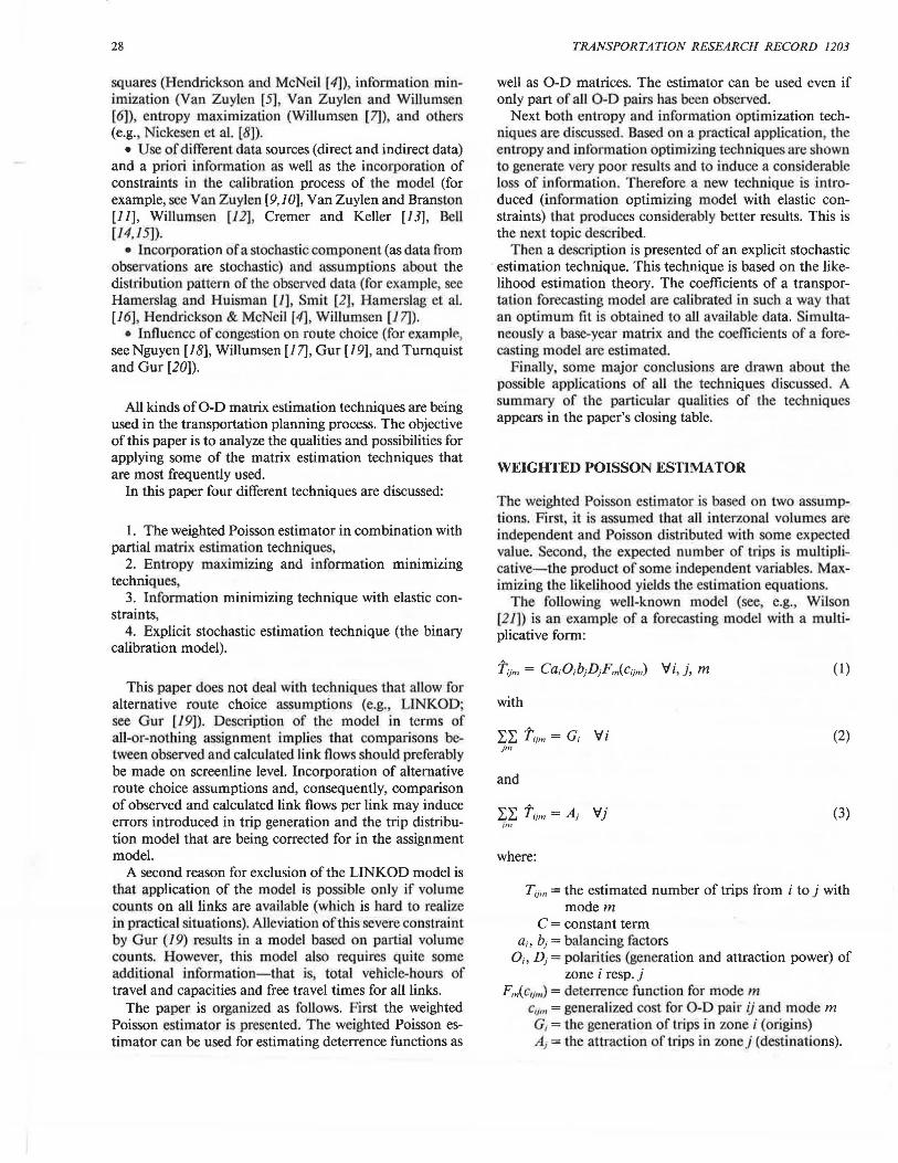
squares (Hendrickson and McNeiJ (4)) information min­imization (Van Zuylen [5], Van Zuylen and Willumsen [6]) entropy maximization (Willumsen [7]), and others (e.g., Nickesen et al. [8]).

• Use of different data sources (direct and indirect data) and a priori information as well as the incorporation of constraints in the calibration process of the model (for example, see Van ZuyJen (9, 1 O], Van Zuylen and Branston [Jl], Willumsen [12] , Cremer and Keller [13], Bell (/4,15)).

• incorporation ofa stochastic component (as data from observations are stochastic) and assumptions about the distribution pattern of the observed data (for example, see Hamerslag and Huisman [J], Smit (2], Hamerslag et al. [16], Hendrickson & McNeil [4], Willumsen (17]).

• Influence of congestion on route choice (for example, see Nguyen (18], Willumsen [17], Gur [19], and Turnquist and Gur [20]).

All kinds ofO-D matrix estimation techniques are being used in the transportation planning process. The objective of this paper is to analyze the qualities and possibilities for applying some of the matrix estimation techniques that are most frequently used.

In this paper four different techniques are discussed:

1. The weighted Poisson estimator in combination with partial matrix estimation techniques,

2. Entropy maximizing and information minimizing techniques,

3. Information minimizing technique with elastic con­straints,

4. Explicit stochastic estimation technique (the binary calibration model).

This paper does not deal with techniques that allow for alternative route choice assumptions (e.g. LINKOD· see Gur [19]). Description of the model in terms of all-or-nothing assignment implies that comparisons be­tween observed and calculatedJink flows should preferably be made on screenline level. Incorporation of alternative route choice assumptions and, consequently, comparison of observed and calculated link flows per link may induce errors introduced in trip generation and the trip distribu­tion model that are being corrected for in the assignment model.

A second reason for exclusion of the LINKOD model is that application of the model is possible only if volume counts on all links are available (which is hard to realize in practical situations). Alleviation of this severe constraint by Gur (19) results in a model based on partial volume counts. However, thi model also requires quite some additional information- that is total vehicle-hours of travel and capacities and free travel times for all links.

The paper is organized as follows. First the weighted Poisson estimator is presented. The weighted Poisson es­timator can be used for estimating deterrence functions as

TRANSPORTATION RESEARCH RECORD 1203

well as 0-0 matrices. The estimator can be used even if only part of all 0-D pairs has been observed.

Next both entropy and information optimization tech­niques are discussed. Based on a practical application, the entropy and information optimizing techniques are shown to generate very poor results and to induce a considerable loss of information. Therefore a new technique is intro­duced (information optimizing model with elastic con­straints) that produces considerably better results. This is the next topic described.

Then a description is presented of an explicit stochastic - estimation technique. This technique is based on the like­lihood estimation theory. The coefficients of a transpor­tation forecasting model are calibrated in such a way that an optimum fit is obtained to alJ available data. Simulta­neously a base-year matrix and the coefficients of a fore­casting model are estimated.

FinalJy, some major conclusions are drawn about the possible applications of all the techniques discussed. A summary of the particular qualities of the techniques appears in the paper's closing table.

WEIGHTED POISSON ESTIMATOR

The weighted Poisson estimator is based on two assump­tions. First, it is assumed that all interzonal volumes are independent and Poisson distributed with some expected value. Second, the expected number of trips is multipli­cative-the product of some independent variables. Max­imizing the likelihood yields the estimation equations.

The following well-known model (see e.g., Wilson [21]) is an example of a foreca ting model with a multi­plicative form:

(1)

with

LL Tum= G; Vi (2) pn

and

LL Tum= A1 VJ (3) im

where:

Tu111 = the estimated number of trips from i to j with modem

C = constant term a;, b1 =balancing factors

O;, D1 =polarities (generation and attraction power) of zone i resp. j

Fm(C1;,,,) =deterrence function for modem c,",, = generaHzed cost for 0-D pair ij and mode m G, =the generation of trips in zone i (origins) A1 =the attraction of trips in zone j (destinations).

Hamerslag and lmmers

Let us assume

(4)

and

(5)

where Cijm belongs to generalized cost class k.

Substitution of formulas 4 and 5 in formula 1 yields

't;jm = CoAFmk Vi, j, m (6)

29

The result is a set of nonlinear equations with which the coefficients can be determined using an iterative method, such as the Gauss-Seidel principle.

(14)

(15)

LL Tum I)

FA _ _,cu="'-ek__ V k "'k - LL Co,a1 m, (16)

lj

The probability of observing Tijm trips can be given by the and equation

(7)

where T ijm = estimate of T ijm·

The number of trips Tv,,, is assumed to be independent for all combinations of ij, and m. As a result the value of the log-likelihood function (L *) becomes

L* = ln(L) = LL ln(Pr[Tijm I Tum]) ij

(8)

The coefficients in formula 1 should be chosen in such a way that the log-likelihood has a maximum value. Sub­stitution of formulas 1 and 7 in 8 yields the log-likelihood function:

L * = LL l(-Co;aJ1mk) ij

+ Tum[ln(C) + ln(o;) + ln(aj) + ln(Fmk)]

- ln(Tuml)I (9)

The maximum value of the log-likelihood is found by setting the first partial derivatives to zero:

oL* Vi -=0 (10)

00;

oL* Vj (11) --o

o~ -

oL* Vm, k (12) ~=O

oFmk

oL* (13) -=0

oC

(17)

This set of equations can be solved only if there are no inconsistencies in the data. In general this condition will not be fulfilled if data from more than one home interview or from various cordon interviews are used.

The weighted Poisson estimator was applied for the first time in the early 1970s. At first the model was used for estimating deterrence functions (Evans and Kirby [22], Hamerslag [23]}. Since then, the model has also been used for estimating 0-D matrices, even if only a part of all 0-D pairs has been observed. For that reason, the model is especially suited for making estimates using survey data from cordon interviews. An estimate of unobserved 0 -D pairs in the matrix can be obtained using partial matrix techniques (Neffendorf and Wootton [24]). This applica­tion of the model, however is not always without problems (see, for example, Day and Hawkins [25], Kirby and Murchland [26]). Information from road traffic counts or public transport ridership cannot be used as it lacks 0-D information. The weighted Poisson estimator is also used for the analysis of multidimensional matrices (Hamerslag et al. [27]).

ENTROPY MAXIMIZING AND INFORMATION MINIMIZING MODEL

According to information theory, the most likely trip matrix is a matrix that can arise in the greatest number of ways and that satisfies whatever constraints are placed on the system. The entropy maximizing (EM) and informa­tion minimizing (IM) models are equivalent; the only difference between them is that the latter makes use of some initial knowledge about the likely trip matrix (an a priori matrix). The IM model is a generalization of the EM model.

30

If only the total number of trips in the system is known, the entropy maximizing method will distribute these trips evenly over all cells of the matrix. Adding some constraints might result in a more realistic picture. Wilson (28) for example, subjected the entropy to the following con­straints: the total number of origin and destination trips per zone and a general function of distance (e.g., general­ized cost). The result is a conventional, double-constrained gravity model with an exponential deterrence function. It is also possible to incorporate some extra information into the model-for example, the observed link flows (link counts Va per direction). It should be noted, however, that each link count (Va) adds an extra constraint to the esti­mate that results in an extra Lagrange multiplier and, consequently, an extra coefficient in the model. Of course, it is also possible to make au estimate of a trip matrix without using information that is essential in the conven­tional gravity model (e.g., the average distance traveled).

The EM model for the estimation of trip matrices from traffic counts was introduced by Willumsen (7). Van Zuylen (9) derived the IM model. An attractive feature of Van Zuylen's model is the possibility of incor­porating extra information (an a priori trip matrix) that might result in a more realistic estimate of the actual trip matrix. Later the possibility of incorporating extra a priori information is also introduced in the EM model. The better the a priori matrix, the better the estimate will be. An old 0-D matrix might be well suited for use, but it is also possible to use an 0-D matrix estimate from the weighted Poisson model (see preceding section) or a Wilson type of model as a first guess.

Formulation of the Information Minimizing Model

According to the information minimizing theory (Van Zuylen [9]), the most likely trip matrix Tu satisfies the following equation:

L =min :L~ [Tuln(~)] TIJ U J. fj

(18)

subject to

LL (Tud'ij) =Ra Va (19) 1j

where

L ="distance" between matrices Tu= the number of trips frum i to j (to be estimated

a posteriori) R., =constraint a (e.g. traffic count, total number of

arrivals per zone, trip length distribution, etc.) dij = the fraction of trips ij subjected to constraint R,,

(e.g., the number of trips ij that make use of link a)

Tu = a priori matrix. This matrix is based on some initial knowledge (old 0-0 matrix or model esti­mate).

TRANSPORTATION RESEARCH RECORD 1203

If Tu = 1, Equation 18 is equivalent to the entropy maximizing formulation.

Minimizing the information of Equation 18 subject to the constraints of 19 gives an estimate for Tu. The solution can be derived by minimizing the Lagrangian (if the Kuhn-Tucker conditions are fulfilled)

(20)

The solution is found by setting the partial derivatives to zero

~ = 0 Vij f>Tu

l'!L = 0 Va fiAa

Equation 21 yields

fJL A ( ) ~ = 1 + ln(Tu) - ln(Tu) - L Aa LL dij = 0 (JJ 1J a IJ

Suppose

ln(X0 ) = -1 ln(Xa) = Aa LL dij ij

Substitution in Equation 23 yields

Tu= TuXo II Xa Vi, j a

where

LL (Tudij) =Ra Va ij

(21)

(22)

(23)

(24)

(19)

Equation 24 shows that the a priori information (0-D matrix) is multiplied by a number of coefficients X,,. Each constraint {R,,) introduces an extra coefficient X,, into the model. An important difference between the IM and EM models is that in case of more observations (N} per 0-D pair, there i& a positive correlation betw~~n the hias of the EM estimate and the number of times the flow is counted; the IM estimate is free of bias (see Maher [29]).

The model described earlier has some specific charac­teristics:

• The amount of traffic (Tu) is estimated using a model with coefficients that are time- and place-dependent. A change in the volume counts will result in a change of the coefficients (Lagrange multipliers) of the model.

Hamerslag and Immers

• Equation 18 is not defined in case Tu= 0. All relations of the trip matrix Tu that are not observed cannot be used in the estimation process. This may become a severe problem if an observed a priori 0-D matrix is used that (in most cases) contains, for the greater part, zero values. All 0-D pairs that are not observed should be estimated first, for example, by using the weighted Poisson model (see preceding section).

• If the set of constraints in Equation 19 contains in­consistencies, no feasible solution will be found. To be able to solve this problem, it is necessary to remove all inconsistencies from the data and to estimate the trip matrix from the consistent flows (see Van Zuylen [9), Van Zuylen and Willumsen [6]). This problem often occurs, especially if cordon surveys are used in which 0-D pairs might be observed several times. Therefore, some tech­niques have been developed to cope with this problem (see, e.g., Roos [30] Ellis and Van Ammers [31], and Smit and Te Linde [32)).

2511 245 2411 235 2311 225 2211 215 2111 2115 21!11 195 191! 185 1811 175 1711 165 160 155 159 145 1411 135 139 125 121! 115 119 11!5 11111

0 0

0

0

0

0

0

0

D

0

D

0

95 91! 85 811 75 78 65 611 55 511 45 49 35 311 25 211 15 111

D D °/ Dq, oJ

5 II

e

DO 0 0 i§l / 0 00 r! 0 0 /. D 0

0 8 tfl Do a /' o

0 0 t:fq 0 ~ 0 D 0 Cl:iC!Q 0 D D

0 0 8dJO D \0 DO ocP..

8 o

0 0 D 0

0

25 59 75

31

To improve the estimation technique, the entropy maximizing model has been extended in several ways­for example, the incorporation of a route information component (Van Maarseveen and Ruygrok [33], Van Maarseveen et al. [34], Willumsen [12)), as well as the introduction of time-dependent trip matrices (Willumsen [17]).

Loss of Information

Van Vuren [35] used the IM model to estimate an 0-D matrix of bicycle trips in Delft. The a priori information consisted of an 0-D matrix of partly observed, partly modeled trips; bicycle counts were added as extra infor­mation. As can be seen from Figure I, the model estimate (a posteriori matrix) differed considerably from the a priori matrix, which indicates that quite some a priori informa­tion got lost.

/

0

0 0

0

/

0

D

.tllll

/ /

/

/

D

D

125 1511 175

FIGURE 1 Random sample of the a priori and a posteriori values of 0-D pairs estimated using the information minimizing model (35).

32

The tremendous change in the trip matrix might have been caused by the following factors:

• incorrect a priori matrix, • specific properties of the information minimizing

model, • inconsistent data.

Unfortunately, it is not possible to trace the effects of all factors. However, an indication of the effects of the specific properties of the model can be given using the following example in which the model as been applied to a small network. The network is shown in Figure 2. Trips are generated between the zones 1, 2, 3, and 4 only. The observed trip pattern (Tu) is shown in Table 1. This trip matrix will be used as a priori information. The assignment of all trips to the network results in link flows as indicated with C (calculated) in Figure 2.

The observed link flows are indicated with 0. There is some dissimilarity between the calculated and observed flows, but the deviations are kept within bounds. As is usual in practice, only the network flows on a limited number of links are observed.

O= 80 C=100

FIGURE 2 Observed (0) and calculated (C) link flows. Calculated link flows are based on assignment of observed 0-D matrix (Table 1).

3

4

TRANSPORTATION RESEARCH RECORD 1203

The results of the estimation of the 0-0 matrix using the information minimizing model are also shown in Table 1; the calculated flows are shown in Figure 3. As can be seen from Figure 3, the observed and calculated network flows are practically identical, which implies that there are no inconsistencies in the data. Otherwise, no feasible so­lution would have been obtained. A closer look at Table 1, however, makes it evident that the estimated 0-D matrix has changed considerably.

This example clearly illustrates that because of the nec­essary adjustments that had to be made to meet the link flow constraints, the information stored in the a priori matrix has changed considerably.

In fact, the entropy maximizing model as introduced by Willumsen ( 7) will render almost the same results. The introduction of constraints with regard to the total nnmher of incoming and outgoing flows per zone as well as the total distance traveled will result in the entropy model as formulated by Wilson. This very model, however, can also be considered an a priori matrix. The incorporation of extra constraints will modify the results of the estimation process in the same way as has already been indicated (except for the adaptation to the incoming and outgoing

O= 80 C= 80

FIGURE 3 Observed and calculated link flows using the information minimizing model.

4

TABLE 1 OBSERVED (A PRIORI MATRIX TiJ) AND ESTIMATED (TiJ) 0-D MATRIX USING THE INFORMATION MINIMIZING MODEL

from to 2 3 4

Tij Tij Tij Tij Tij Tij Tij Tij 1r1J ~Tij

10 27 40 30 10 11 60 68

2 10 31 40 28 10 10 60 69

lO 6 10 5 IO 19 30 30

4 10 10 IO 8 40 81 60 99

P1J;F1j 30 47 30 40 l20 l39 30 40 210 266

Hamerslag and lmmers

flows per zone). Figure l, being the result of a practical application of the model, clearly shows which adjustments in the a priori matrix were necessary to cope with all constraints. Actually the model formulation places less importance or less confidence in the a priori information. The concept of giving weights (e.g., in accordance with the reliability of different types of information) might be more appropriate.

INFORMATION MINIMIZING MODEL WITH ELASTIC CONSTRAINTS

The example in the preceding section clearly indicates that application of the information minimizing model may lead to considerable loss of information. The reason for this (unexpected) result can be found in the omission of the stochastic properties of the constraints (traffic counts and the like). All constraints that are incorporated into the model behave deterministically. To solve this problem of "information loss," it is suggested that the model be refor­mulated using elastic instead of fixed constraints (analo­gous to the transportation model with elastic constraints; Hamerslag [23]).

Model Specification

Application of elastic constraints in the optimization prob­lem yields the following equations:

Tu= TuXo II Xa Vi, j (24) a

LL (Tud'ij} = Sa Va (25) I}

(26)

So Equation 19 is replaced by Equations 25 and 26. But in case ga = 0, Sa equals R 0 •

In case of a constraint b, substitution of Equations 24 and 25 in 26 yields the following equation:

(TX II (X )db) x-gb Rb = x b L_L I} 0 a a I}

I] a>"'b

(27)

which, after some conversion results in:

{

Rb } 11<1+gb>

xb = LL TuXd II (Xa)dt IJ a

a,.b

(28)

The exponent [1/(1 + gb)] in Equation 28 is defined as the elasticity of constraint b. If the elasticity [ l /(l + gb)]

33

equals 0, then Xb = 1, which implies that constraint b does not have any influence on the model estimate. If the elasticity [1/(1 + gb)] equals l, however, the model estimate will correspond completely with constraint b. In the latter case, the information minimizing model is being dealt with.

An interesting feature of the model with elastic con­straints is that (choosing correct values of the elasticities) the loss of a priori information that will occur has been reduced considerably. This can easily be demonstrated using the example given earlier. The results of an applica­tion of the model using an overall value of the elasticities of0,5 are shown in Figure 4 and Table 2.

As can be seen from Table 2 the estimated 0-D matrix is very similar to the a priori matrix; this implies that the information stored in the a priori matrix influences the model estimate (no loss of information). Still some differ­ences between the observed and calculated link flows will remain. This phenomenon is completely in accordance with the nature of observed link flows, however, showing quite a bit of variation over time. Therefore the amount of extra information added to the problem by observed link flows (traffic counts) is limited; consequently, the application of fixed constraints would be erroneous.

The estimate of the 0-D matrix strongly depends on the values of the elasticities (as is shown in Table 3), especially for values close to J. Although it is not yet possible to give a clear indication of which values should be given to the elasticities of the constraints, it is obvious that two factors are predominant:

• the additive amount of 0-D information and • the reliability of the information.

Apart from these factors, it is obvious that the values of the elasticities should be chosen in such a way that the sum (or weighted sum) of chi2 (for flows and 0-D pairs) has a minimum value. (See Figure 5 and Table 4.)

As has been shown, the application of the information­minimizing model with elastic constraints might improve

O= 80 C=101

FIGURE 4 Observed and calculated link flows using the information minimizing model with elastic constraints.

3

4

34 TRANSPORTATION RESEARCH RECORD 1203

TABLE 2 OBSERVED (A PRIORI MATRIX Tu) AND ESTIMATED (Tu) 0-D MATRIX USING THE INFORMATION MINIMIZING MODEL WITH ELASTIC CONSTRAINTS

from to 2

Tij Tij Tij Tij

elasticity - 0,5 0,5

10 13

2 10 11

3 10 9 10 11

4 10 10 10 11

F1j;'i_T1j 30 30 30 35

considerably the estimate of an 0-D matrix using a priori information and traffic counts. Nevertheless, some short­comings (some of them indicated in the section on the weighted Poisson estimator) will remain:

• Each observation is formulated as a constraint and consequently results in the incorporation of an extra coef­ficient in the estimation model. These coefficients are time- and place-dependent, which precludes the possibility of using the model for predicting medium- to long-term changes.

• The estimated 0-D matrix depends heavily on the values of the elasticities (see Table 3). If those values equal 0, the a priori matrix will not change. A value of the elasticities equal to 1 will result in the information mini­mizing model.

• The available information from traffic counts is used to fit only those 0-D pairs that pass along the observed links. All other 0-D pairs will not change at all. This problem can be overcome by using additional 0-D infor­mation-for example, trip distance distribution.

BINARY CALIBRATION MODEL

The use of traffic data for estimation (calibration) purposes requires some caution. The continuous variation of traffic flows, the availability of data from various sources (sur­veys, counts ticket sales), as well as differences in sample size and observed population groups may result in a con­siderable amount of stochasticity. Especially if various

3

Tij

40

40

40

120

4

-Fij 1Tij Tij Tij Tij

0,5 0,5

40 10 11 60 64

40 10 11 60 62

10 11 30 )1

45 60 66

125 30 33 210 223

kinds of survey data are used because of this stochasticity, some inconsistencies in the data may show up (the data seem to be contradictory). In general, use of various data sources does not raise any problems; it is also possible (especially in case of inconsistencies), however, for no feasible solution to be found. The latter is especially true for the entropy type of model. Estimation models do exist, however, that can deal with the stochastic properties of the observations. Like the entropy model, all coefficients are calibrated in such a way that an optimum fit will be obtained between the observed data and the estimated trip matrix. One essential difference, in contrast to the entropy type of model, is that no additional coefficients are intro­duced to meet all constraints.

Hamerslag and Huisman (J) formulated the binary cal­ibration model, which is based on the assumption that the observed data are independently Poisson distributed.

Smit (2) and Hendrickson and McNeil (4) use a normal distribution. Use of both latter models may raise some problems because they allow for negative flows (especially in case of relatively small flows).

Model Formulation

Suppose Tu is the available a priori information (e.g., an old, observed 0-D matrix). Instead of using an observed 0-D matrix, it is preferable to use estimates of Tu (e.g., an estimate of Tu using the weighted Poisson model).

An advantage of the use of estimates is that the 0-D matrix Tu will not contain zero values. Analogous to

Hamers/ag and Immers 35

TABLE 3 ESTIMATE OF 0-D MATRIX FOR DIFFERENT VALUES OF THE ELASTICITIES

from to 2

elasticities

o.o 10

o.s 13

0.8 17

0.9

1.0

2 10

11

15

19

31

3 10 10

9 11

8

8

6

4 10 10

10 11

10

10

10

Equation 6 such a matrix can be formulated as follows:

(29)

where

Tu= number of trips from i to j (model estimate or a priori matrix)

C = constant term O; = a;O; = product of balancing factor and polarity of

zone i cl = bjDj = product of balancing factor and polarity of

zone} Fk = value of deterrence function for a generalized cost

class k and cu E k.

10

12

20

8

11

27

5

8

3 4

40 10

40 11

37 11

34 11

30 11

40 10

40 11

38 11

35 11

28 10

10

11

13

15

19

40

45

55

63

81

Let us further assume

Ya= information from observations (a) (e.g., depar­tures, arrivals per zone, traffic counts, trip distance distribution, etc.)

dij =a binary variable indicating whether 0-D pair ij belongs to observation a (dij = 1) or not (dij = 0)

ano

Ya ~ LL (Tud't) (30) u

The relation between the estimate of the base year matrix (Tu) and the a priori matrix can be represented by

36 TRANSPORTATION RESEARCH RECORD 1203

-Flows ----· 0-D matrix--- -- Sum

80

70

I 60

50 (\I

:f 40 t)

30

20

10

0 ----------------- ---

0 .5 .6 .7 .8 ,9 1.0

Elasticities

FIGURE 5 Chi-square for different values of the elasticities.

TABLE 4 OBSERVED (A PRIORI MATRIX Tu) AND ESTIMATED (Tu) 0-D MATRIX USING THE BINARY CALIBRATION MODEL

from to 2 3 4

. Tij Tij Tij Tij Tij Tij Tij Tij ]Tij ]Tij

10 10 40 40 10 12 60 62

2 10 10 40 40 10 12 60 62

3 10 10 10 9 10 11 30 30

4 10 11 10 11 40 40 60 62

. F1j;1i_T1j 30 31 30 30 120 120 30 35 210 216

the following equation: The logarithm of the likelihood yields

(31) ln(L) = L* = -L (.Ya)+ L [Ya ln(Ya)] a a

where i E /, j E J, and k E K. - L [ln(Ya!)] a

(34)

The preceding formulation implies that sets of balancing factors as well as discrete values of the deterrence function are modified; however, the general form of the model remains unchanged.

An optimum adjustment between Ya and Ya can be determined by maximizing L * or as

Assuming that the observations (Ya) are independent and Poisson distributed, the likelihood (L) can be deter­mined as follows:

Pr[Ya I Ya]= exp(-Ya)(Yar">/Ya!

L = II (Pr[ Ya I Ya]) a

(32)

(33)

L [ln(Ya!)] = constant a

by maximizing

(35) a a

Hamersfag and Immers

O= 80 C=104

37

3

4

FIGURE 6 Observed and calculated link flows using the binary calibration model.

which yields the following equations:

L [ ( :u _ 1) o Ya] = O a Ya 001

VI (36)

L [ ( ~ - I) o Ya] = 0 u Ya odJ VJ (37)

}: [ ( ~ - 1) o Ya] = 0 a Yu oFK VK (38)

L[(:a_ 1)oYa]=O a Ya oC (39)

The values of 01 , dh Fk, and C will be determined itera­tively (anaJogous to the Gauss-Seidel principle). Inserting those values in Equation 31 yields the estimates for the base year matrix t i/.

Application of the Model

The results of a practical application of the binary calibra­tion model using the same example as before (network, a priori information, and link traffic counts) are shown in Figure 6 and Table 4.

It can be noted from Table 4 that the trip matrix estimate (Tu) is practically equivalent to the observed a priori matrix. It can also be noted from Figure 6 that all link traffic flow estimates are not equivalent to the link traffic counts, but there is a great similarity. Both results corre­spond to the very nature of the data used in the estimation process (see also the preceding section on information optimizing with elastic constraints).

The advantage pf using the binary calibration model, especially compared to the information minimizing model with elastic constraints, is that no extra coefficients are incorporated in the model that allows use of the model for making medium- and long-term forecasts.

CONCLUSIONS

This paper deals with four models that can be used for estimating an 0-D matrix:

• the weighted Poisson estimator • the entropy maximizing and information minimizing

model • the information minimizing model with elastic con­

straints • the binary calibration model

The weighted Poisson model is especially well suited for estimating deterrence functions and a base year matrix using information from household or cordon surveys (only 0-D information). This base year matrix estimate is espe­cially appropriate for use in the information minimizing model with elastic constraints or the binary calibration model (the base year matrix estimate is treated as a priori information).

The entropy maximizing and information minimizing models show some severe shortcomings. First, neither model allows for inconsistent information. Second, all coefficients in the model are time- and place-dependent, which precludes the possibility of using the models for making medium- and long-term forecasts. And, last but not least, use of both models induces loss of information.

The latter problem can be resolved using a model with elastic instead of fixed constraints. As has been shown, the values of the elasticities strongly influence the estimate and, consequently the loss of information. Besides, the available information from traffic counts is used only to fit those 0-D pairs that pass along the observed links. AU other 0-D pairs will not change at all.

The binary calibration model does not show any of the shortcomings just mentioned. The model, however, has a rather complex structure and has been successfully applied in the Netherlands (see, e.g., Haroerslag et al [16) and Heere and Huisman [36]). -

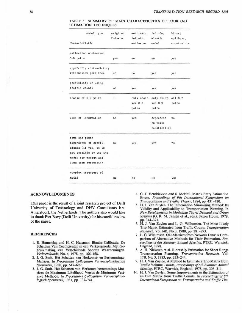
Table 5 presents a summary of the main characteristics of the models dealt with in this paper.

38 TRANSPORTATION RESEARCH RECORD 1203

TABLE 5 SUMMARY OF MAIN CHARACTERISTICS OF FOUR 0-D ESTIMATION TECHNIQUES

model type

characteristic

estimation unobserved

C>-D pairs

apparently contradictory

information permitted

possibility of using

traffic counts

change of C>-D pairs

loss of information

time and place

dependency of coef f i­

cients (if yes, it is

not possible to use the

model for medium and

long term forecasts)

complex structure of

model

ACKNOWLEDGMENTS

weighted

Poisson

yes

no

no

no

no

no

This paper is the result of a joint research project of Delft University of Technology and DHV Consultants b.v. Amersfoort, the Netherlands. The authors also would like to thank Piet Bovy (Delft University) for his careful review of the paper.

REFERENCES

I. R. Hamerslag and FI. C. Huisman. Binaire Calibratie. De Scbauing Van Coefficienten in een Verkeersmodel Met Ge­bruikmaking van Verschillende Soorten Waarnemingen. Verkeerskunde, No. 4, 1978, pp. 166-168.

2. J. G. Smit. Het Scbatten van Herkomst- en Bestemmings­Matrices. In Proceedings Colloquium Vervoersplanologisch Speurwerk, 1980, ·pp. 647-699.

3. J. G. Smit. Het Schatten van Herkomst-bestemmings Mat­rices: de Maximum Likelihood Versus de Minimum Vari­ance Methode. In Proceedings Colloquium Vervoersplano­logisch Speurwerk, 1981, pp. 737-741.

entr.max. inf.min . binary

calibrat. inf.min. elastic

estimator model constraints

no no yes

no yes yes

yes yes yes

only obser- only obser- all 0-D

ved C>-D ved C>-D pairs

pairs pairs

yes dependent no

on value

no

elasticities

nc

no yes

4. C. T. Hendrickson and S. McNeil. Matrix Entry Estimation Errors. Proceedings of 9th lnlemational Symposium on Transportation and .Traffic Theory, 1984, pp. 431-430.

5. H. J. Van Zuylen. The Information Minimising Method: Its Validity and Applicability to Transportation Planning. In New Developments in Modelling Travel Demand and Urban Systems (G. R. M. Jansen et al., eds.) Saxon House, 1979, pp. 344-371.

6. H. J. Van Zuylen and L. G. Willumsen. The Most Likely Trip Matrix Estimated from Traffic Counts. Transportation Research, Vol14B No.3, 1980, pp. 281 - 293.

7. L. G. Willumsen. OD-Matrices from Network Data: A Com­parison of Alternative Methods for Their Estimation. Pro­ceedings of 6th Summer Annual Meeting, PTRC, Warwick England, 1978.

8. A. H. Nickesen et al. Ridership Estimation for Short Range Transportation Planning. Transportation Research, Vol. 17B, No. 3, 1983, pp. 233-244.

9. H. J. Van Zuylen. A Method to Estimate a Trip Matrix from Traffic Volume Counts. Proceedings of 6th Summer Annual Meeting, PTRC, Warwick, England, 1978, P.P· 305-311 .

10. H. J. Van Zuylen. Some Improvements in the Estimation of an 0-D Matrix from Traffic CountS. In Proceedings of 8th International Symposium on Transportation and Traffic The-

Hamerslag and Immers

ory (V. F. Hurdle et al., eds.), Toronto, Ontario, Canada, 1981, pp. 183-190.

11. H. J. Van Zuylen and D.M. Branston. Consistent Flow Estimation from Counts. Transportation Research, Vol. I 6B, No. 6 1982, pp. 473-476.

12. L. 0. Willumsen. Estimation ofTrip Matrices from Volume Counts: Validation ofa Model Under Congested Conditions. Proceedings of 10th Summer Annual Meeting, PTRC, Semi­nar Q, Warwick, England, 1982, pp. 311-324.

13. M. Cremer and H. Keller. A Systems Dynamics Approach to the Estimation of Entry and Exit 0-D Flows. Ju Proceed­ings of 9th International Symposium on Transportation and Trqffic Theory (1. Volmuller and R. Hamerslag, eds.), Delft, VNU-Science Press, Utrecht, Nethedands, 1984 pp. 431-450.

14. M. 0 . H . Bell. The Estimation of an Origin- Destination Matrix from Traffic Counts. Transportation Science, Vol. 17 No. 2, 1983, pp. 198-2 17.

15. M . G. H . Bell. The Estimation of Junction Turning Volumes from Traffic Counts: The Role of Prior Information. Traffic Engineering and Control, Vol. 25, No. 5, 1984, pp. 279- 283.

16. R. Hamerslag et al. Een Toepassing van Binaire Calibratie in een Regionale Studie. Proceedings Colloquium Vervoer­spla11ologisd1 Speurwerk, 1981 , pp. 713-735.

17. L. G . Willumsen. Estimating Time-dependent Trip Matrices from Traffic Counts. Proceedings of 9th International Sym­posil.un on Transportation and Trqffic Theory, 1984, pp. 377-411.

18. S. Nguyen. 011 the Estimation of an 0 -D Trip Matrix by Eq11ilibrium Methods Using Pseudo-delay Funclions. CRT­publ. 81. Universite de Montreal, Centre de Recherche sur Les Transports Montreal, Quebec Canada, 1978.

19. Y. J . Our. Trip Table Estimation Based on Partial Volume Counts. Paper Presented at 64th Annual Meeting, TRB, January 1985.

20. M. Turnquist and Y. Our. Estimation of Trip Tables from Observed Link Volumes. Transportation Research Record 730, TRB, National Research Council, Washington, D.C., 1981, pp. 1-6.

21. A. 0. Wilson. The Use of Entropy Maximising Models in the Theory of Trip Distribution, Modal Split and Route Split.. Joumal of Transport Economics and Policy, Vol. 2, No. 1, 1969, pp. 108-126.

22. S. F. Evans and H. R. Kirby. A Three Dimensional Furness Procedure for Calibrating Gravity Models. Presented at PTRC Summer Annual Meeting, Warwick, England, 1973.

23. R. Hamerslag. Transportation Model with Elastic Con­straints. Proceedings of 2nd PTRC Summer An1111al Meeting, Warwick England, 1974.

39

24. H. Neffendorfand H.J. Wootton. (1974): A Travel Estima­tion Model Based on Screenline Interviews. Proceedings of 2nd Swnmer Annual Meeting, PTRC, Warwick, England, 1974.

25. M. J. L. Day and A. F. Hawkins. Partial Matrices, Em­pirical Deterrence Functions and Ill Defined Results. Traffic E11gineeri11g and Control, 1979, pp. 429-433.

26. H. R. Kirby and J. D. Murchland. Gravity Model Fitting with Both Origin- Destination Data and Modelled Trip-end Estimates. Proceedi11gs of 8th International Symposium on Transportation and Traffic Theory, Toronto, Ontario, Can­ada, 1981.

27. R. Hamerslag. Het Schatten van Herkomst- en Bestemmings­matcices m.b.v. Schijnbaar Tegenstrijctige Waamemiogen. Proceedings Colloquium Vervoersp/ano/ogisch Spe11nverk 1980, pp. 711-714.

28. A. 0. Wilson. A Statistical Theory of Spatial Distribution Models. Transportation Research, 1967, pp. 253-269.

29. M. J . Maher. Bias in the Estimation ofO-D Hows from Link Counts. Paper presented at UTSO conference, Sheffield, United Kingdom, 1987.

30. J . P. Roos. Het Gebruik Van Verkeerstellingen en Wegenen­quetes bij bet Opstellen van HB-tabelJen. Proceedings Col­loquium Vervoersplanologisch Speurwerk 1982, pp. 421-431.

31. M. C. Ellis and H. Van Ammers. Forecasting Using Cordon Surveys in the Egyptian National Transportation Study. Pro· ceedings of 9th Summer Annual Meeting, PTRC, Warwick, England, 1981.

32. J. G . Smit and J. Te Linde. Dubbelenquetes. Proceedings Colloquium Vervoersplanologisch Speurwerk, 1982, pp. 375-395.

33. M. F. A. M. Van Maarseveen and C. J. Ruygrok. Het Oebruik van Route-informatie V oor het Opstellen van HB-matrices. Proceedings Colloquium Vervoersplanologisch Speurwerk, 1982, pp. 399-420.

34. M. F. A. M. Van Maarseveen et al. Estimating 0-D Tables Using Empirical Route Choice Information with Application to Bicycle Traffic. Paper presented at 64th Annual Meeting, TRB, January 1985.

35. T. Van Vuren. Het Schatten van een Herkomst- en Bestem­mingstabel: Een Overzicht. Thesis. Delft University of Tech­nology, Delft, Netherlands, 1985.

36. E. Heere and M. C. Huisman. Toepassing van de binaire Calibratiemethode in Zaanstad. Verkeerskunde, 1978, pp. 239-242.

Publication of this paper sponsored by Committee on Passenger Travel Demand Forecasting.