Estimation theorySenaka Samarasekera

SS

P a

lgorith

m

develo

pm

en

t pro

cess

Problem statement

Specifications

Model information

and Raw-data

acquisition

Solution

Sensitivity analysisRobust?Field testSpecs met

in the field

Math. model

Specifications Met?

Modify model

Modify m

odel

Best possiblePerfor.

DevelopAlgorithm

Meet specs

Yes

YesYes

No

NoN

o

No

Modify specs/goals

Formulation of the problem

• Selection of a computational structure with well-defined parameters for the implementation of the estimator.• Selection of a criterion of performance or cost function that measures the

performance of the estimator under some assumptions about the statistical properties of the signals to be processed.• Optimization of the performance criterion to determine the parameters of

the optimum estimator.• Evaluation of the optimum value of the performance criterion to determine

whether the optimum estimator satisfies the design specifications.

Formulation of the problem

• Many practical applications (e.g., speech, audio, and image coding) require subjective criteria that are difficult to express mathematically.

• Thus, we focus on criteria of performance that • only depend on the estimation error e (n), • provide a sufficient measure of the user satisfaction, and• lead to a mathematically tractable problem.

• We generally select a criterion of performance by compromising between these objectives.

Estimators

• Estimator : A function of DATA (a.k.a a STATISTIC) that will approximate the ACTUAL VALUE of the PARAMETER in our mathematical model

Scenario 1: Let us observe a DC voltage using a noisy voltmeter. We can model this as

Where is the noise processWe can use the median, or the mean as estimator . Which we will use as an approximation to the true value of the parameter .

Cost of an estimator

• Bias : Systemic error (try to avoid this if possible but not at all costs)

Unbiased estimators B = 0• Variance

Minimum variance estimator arg• Mean-square error

Minimum man square estimator MMSE = arg

Small change in scene 1

• Now lets take an estimator

Find the bias, variance and the that will minimize the mean square error.

Likelihood function

• A pdf parameterized by an unknown parameter • Eg : If noise was Gaussian in the DC measurement case

• What would be the case for multiple observations assuming i.i.d Gaussian noise• A stock of a growing company can be modelled as • where is i.i.d AWGN. What is the likelihood function? Is this

stationary or non stationary?

Assignment 3 question 2• Find the likelihood function of the autoregressive moving average

model

where is a i.i.d zero mean Gaussian noise.

Deterministic vs Random parameters• Deterministic Parameters : Only one value possible but we don’t

know their value. (this lecture) • Random Parameters: An a priori pdf can be defined on the

parameter. This accounts for the prior uncertainty about parameters. Which means parameters are assumed to be random. • In the next lecture we will look at Bayesian methods which will

estimate random parameters.

Estimator development Deterministic parameter case• Least squares estimator• Maximize the Likelihood• Method of moment estimator

No explicit guarantee on the estimator cost optimality. So will have to derive conditions of optimality for these estimators.

• Optimal estimators : Minimizes a suitable average cost function• Unbiased• Minimum variance ( Unbiased)• Minimum mean square error• Mini- max estimators : Minimize the maximum risk : The best in the worst case scenario

Maximum likelihood estimators

MLE

Note that for unimodal likelihood functions

Advantages• Most versatile estimator of the lot• Has a nice physical intuition to it• Has a direct way of finding it• Is consistent – asymptotically unbiased, and asymptotically optimal (w.r.t to mse)), and invariant for

functional transformations • Therefore for large number of observations, MLE-> MVUE

DC level

If we extend this to N observations

DC level example

• Let for be observations from a noisy voltmeter measuring a DC level

Where i.i.d Gaussian with zero mean and unit variance.

What is the maximum likelihood estimator? What if the variance was also Note : For exponential type of likelihood we can maximize the log likelihood function. This helps to avoid overflows that can be quite common in likelihood computations.

Assignment 3 question 3

• A noisy oscillator at a modulator is modeled as

Where is a i.i.d standard Gaussian noise. If the phase offset of the oscillator is a constant for N samples, find an estimator using this N samples.

Numerical determination of the MLE

• For complicated likelihood functions you can use numerical optimization methods such as

Let • Grid search• Newton Rapson

• Scoring method

• Expectation – Maximization

• Warning : Can get stuck in a local maxima. Not guaranteed to get the global maximum.

Expectation – Maximization method

• Uses auxiliary variables to simplify the likelihood. (adding variables simplifies the problem ? )• Let is the unobserved auxiliary variable vector. • This solves the problem by looking at • When is this natural (or effective)• Eg. When we can then we can make which has a nice low dimensional

sufficient statistic

Expectation –Maximization method

For each iteration k, with the input and data x and the likelihood

• Expectation step :FCompute

• Maximization step :

For exponential likelihoods EM method has the properties that

• For real

Optimality of MLE for the linear model• Let the data defined via the general linear model

where and Then the MLE is

This is an efficient estimator as

and the pdf of

Assignment : Prove this

Properties of MLE : Consistency Assuming i.i.d samples

From law of large numbers

Recall

which implies

And RHS of (1) is maximized at . So if take

Properties of MLE : Asymptotic optimality• From the mean value theorem

Since

Assuming IID samples the denominator becomes

Since and

Properties of MLE : Asymptotic optimality• For IID samples the numerator

• Note that are independent random variables too.• Using central limit theorem

But and Var Using Slutsky’s theorem

Invariance properties

• Looks at the MLE of a transformed parameter • If a measurement equation is given by the likelihood function , and if

is one-to-one, then

Method of moments method

Method of moment estimators

• This is a simple estimator that can be used • as it is if the performance is good enough• Or as a stating point to MLE (which would be consistent)

• Let vector of moments of the pdf (likelihood) and be the underlying parameter vector. Then using the pdf definition we can find the function s.t

If is invertible

Now if we plugin the estimators of the respective moments we get the MOM estimators

• The multiple moments needed can be easily found via the moment generation function

Example

• Let the likelihood function be a 2 components Gaussian mixture with unknown variance and weights. Let both means be 0.

Where

Find the MOM estimators

Example

• Let • Let , and Then the parameters (after some algebra) can be shown to be

Minimum variance unbiased estimators (MVUE)

MVUE

Assume two observations with the likelihood functions

Assuming that the MVUE is of the form Find the MVUE if

What if the likelihood function of the second observations changed like

MVUE

• Some time the variance and the bias equations become so complicated that direct optimization methods fail. • Some times no function of data will give a minimum variance for all

possible possible parameter values.

Finding the MVUE

So we use 3 indirect approaches to find MVUE

• Find sufficient statistic. Find unbiased estimator and condition it on the sufficient statistic.• Find CRLB. Select a function form using some other knowledge. Find

parameters that come nearest to the CRLB• Constrain the model to be linear -> BLUE (best linear unbiased)

MVUE I : Sufficient statisticMVUE in the exponential family

Sufficient statistic

• All the information about the parameter in the likelihood function comes through the sufficient statistic.• Note : Raw data it self is a sufficient statistic. • An MVUE should be a function of the sufficient statistic• Minimal sufficient statistic : The smallest of them all ( in dimensions)• Minimal sufficient statistic is always a function of other sufficient

statistics.

Complete statistics

• If the whole parameter set is identifiable using the sufficient statistic these are called a COMPLETE statistic.

• A sufficient statistic is complete iff

• How does this condition relate to parameter identifiability?Note that

Since the only function in the null space of is the function , the space of all possible functions is spanned by the parametric family .

Neyman – Fisher factorization theorem• is a sufficient statistic for the parameter iff we can factor the

likelihood function as

In the DC level observation example find the sufficient statistic1. for the DC level when noise power is known2. for the noise power when 0 dc level3. for the dc level and the noise power

Rao- Blackwell theorem

• Let and two random variables (vectors). Define the conditional expectation on given

Then

Rao – Blackwell theorem proof

• Property 1

• Property 2

≥0 ¿𝟎∴𝑣𝑎𝑟 (𝒚 )≥𝑣𝑎𝑟 𝑔(𝒛 )

Rao–Blackwell theorem applied to estimators• Let

be an estimator of a parameter , then the conditional expectation of given a sufficient statistic

is always a better estimator of , and is never worse.• From a mean square error perspective this means

Lehmann–Scheffé theorem

• If a statistic that is UNBIASED, COMPLETE and SUFFICIENT for some parameter θ, then this statistic has the minimum expected loss for ANY CONVEX LOSS FUNCTION.• In many practical applications with the squared loss-function, it has a

smaller mean squared error among any estimators with the same expected value.• Hence a unbiased, complete, sufficient statistic is a MVUE.

Pitman- Koopman theorem

• Among families of probability distributions whose domain does not vary with the parameter being estimated, only in EXPONENTIAL FAMILY is there a sufficient statistic whose dimension remains bounded as sample size increases • So practically we can find worthwhile minimum sufficient statistics

only for exponential family of distribution.

So what is this magical exponential family?

Exponential family

• Not to be confused with exponential distribution ( it is also a member in this family when the parameter of interest is the mean).• This is concerned with how the pdf’s are parameterized.• A good number of common pdf’s belong to this family when some of

there parameters are knownEg:• Poisson distribution with unknown mean• Exponential distribution with unknown mean• Gaussian distribution with unknown mean/unknown variance/ both mean

and variance unknown

Exponential family

• DefinitionA set of probability distributions admitting following canonical decomposition

Where = sufficient statistic = natural parameters = inner/ dot product = log normalizer = carrier measure

If the observation is a scaler the pdf is UNIVARIATE otherwise if the observation is a vector the pdf is MULTIVARIATE

The ORDER of a member in this family is the DIMENSION OF THE NATURAL PARAMETER SPACE

Example

• Univariate Poisson distribution with unknown meanRecall that the pmf (since is

This can be rearranged to

So

This is a exponential family member of degree 1.

Example

• Find the sufficient statistic, natural parameters, log normalizer, and the carrier measure for the Univariate Gaussian distribution with unknown mean and variance.

Since

Therefore

Exponential Family

Assignment question

• Prove that (a properly normalized) product of arbitrary exponential family members is also a member of the exponential family.• Is it the same for mixtures of exponential family members?

Log-normalizer

• Exponential families are characterized by their strictly convex and differentiable functions F, called log-normalizer or the partition function

Since we have

Log normalizer

• It is also related to the moment generating and cumulant generating functions of the sufficient statistics.

• The moment generating function of the sufficient statistic is

Since the cumulant generating function

Log- normalizer

• Therefore in exponential family we can easily find the mean and the variance of the test statistic as

• The Fisher information of exponential family member also becomes

Assignment question : Prove this

MLE in exponential family

• Taking the log likelihood

Taking the gradient

At saddle points . Therefore the estimators can be found by solving the equation

Which is also the method of moment estimator in this case. Also note that

Is negative showing that log likelihood function is strictly concave, and the saddle point is a maximum.

Assignment questions

• Show that the MLE and MVUE both are efficient in for natural parameters of the exponential family. • Show that Expectation – Maximization method finds the local

maximum of an exponential family joint distribution (of observed and unobserved data)

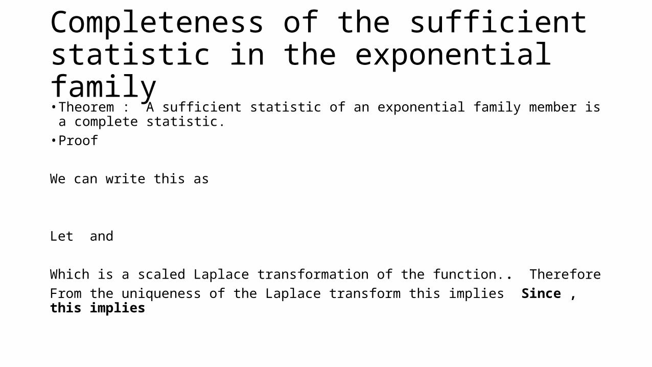
Completeness of the sufficient statistic in the exponential family• Theorem : A sufficient statistic of an exponential family member is a complete

statistic. • Proof

We can write this as

Let and

Which is a scaled Laplace transformation of the function.. Therefore From the uniqueness of the Laplace transform this implies Since , this implies

MVUE II: Best Linear unbiased estimator

Weiner Filter

.

In our compact notation this can be written as

If the number of samples are equal to number of coefficients we can find a that make .

If N > m (which is normally the case) we will try to find that minimize

Weiner Filter

Let us define the ross correlation vector , where each component

uto-correlation matrix where each component

Weiner filter

Now we find an estimate

Where

Applications ofWeiner filter

System identification

Channel equalization

Noise cancellation

BLUE

• Is an extension of the Weiner filtering process. • Now we assume a linear estimator

• To this to be unbiased

For this to be the case for some matrix .If we assume and then

If the covariance matrix of is , then

and

BLUE

• Taking the gradient of each variance and equating it to zero we end up with the BLUE

and

Assignment: Proof: Take each variance and use Lagrange multipliers to enforce . Then minimizing the augmented cost function gives the .Ref: Kay (Appendix 6B pg 153)

Least squares estimators

Least squares estimators (LSE)

• One of the oldest methods going back to Legendre and Gauss• Part of classical regression analysis. • Also known as data/curve fitting • Does not formulate a likelihood function. Just use the signal model

directly.• No probabilistic modeling of the noise.• Cannot claim any probabilistic optimality properties.• Two main classes of problems; Linear/ Non linear Least squares

Linear least square estimators

• For data , parameter estimates and a model (matrix) the squared error function becomes

Taking the gradient

Making it zero to find the maximum

Using this in the squared error equation the minimum error becomes

proof : Kay pg 225

Weighted LSE

• What if we change the error criterion

• When would we use this? All data points are not same• Now

and

• If we add a probabilistic description to the noise which will enable us to formulate a likelihood function then W characterize the spectral characteristic of the noise

Geometrical interpretation

• Let where each column in the model matrix is now viewed as an n dimensional vector.

• If the model is to be identifiable these columns should be independent thus spanning a p-dimensional sub space.

• Lets define the signal estimate ;the signal space approximation of the data.

Eg: Assume , and

• To minimize J the errors should be orthogonal to this p-space.

• Hence minimizing the square error is equivalent to making the error orthogonal to the model

Geometrical interpretation

• What happens if Then the projection on the signal space becomes

Comparing with the earlier result this shows that matrix is unitary as

Geometrical interpretation

• Let’s look at the signal estimate with LSE

• Define the projection matrix , which maps the data to the signal space. • By defining its complement ,we see that the error

and the minimum cost

Sequential least squares estimators

• So far the set of all data points were taken in one single vector . This is called batch processing• What happens if data arrive sequentially? Can we update the LSE

sequentially?E.g. Updating mean

Can we do this to any LSE?

Correction term

Sequential least squares estimators

• Now we index the estimators using the time step

Let us denote where each is a raw vector. Since we can write the Grammian

Sequential least squares estimators

• Note • Since and this can be written as

Since, using the matrix inversion lemma

where

Sequential least squares estimators

• Substituting this to and simplifying we get

Where the correction gain factor